Lin Lin

Computational Research Division, Lawrence Berkeley National Laboratory

Laboratoire Jacques-Louis Lions,

Paris 6, June 2013

Supported by Luis Alvarez fellowship in LBNL, DOE SciDAC and BES Partnership.

1

Fast Algorithms for Electronic Structure Analysis

Acknowledgment Collaborators of past and ongoing projects on this topic: • Roberto Car, Princeton University • Mohan Chen, Princeton University • Weinan E, Princeton University and Peking University • Alberto Garcia, Institute de Ciencia de Materiales de Barcelona • Lixin He, University of Science and Technology in China • Georg Huhs, Barcelona Supercomputing Center • Mathias Jacquelin, Lawrence Berkeley National Laboratory • Juan Meza, UC Merced • Jianfeng Lu, Duke University • Chao Yang, Lawrence Berkeley National Laboratory • Lexing Ying, Stanford University

2

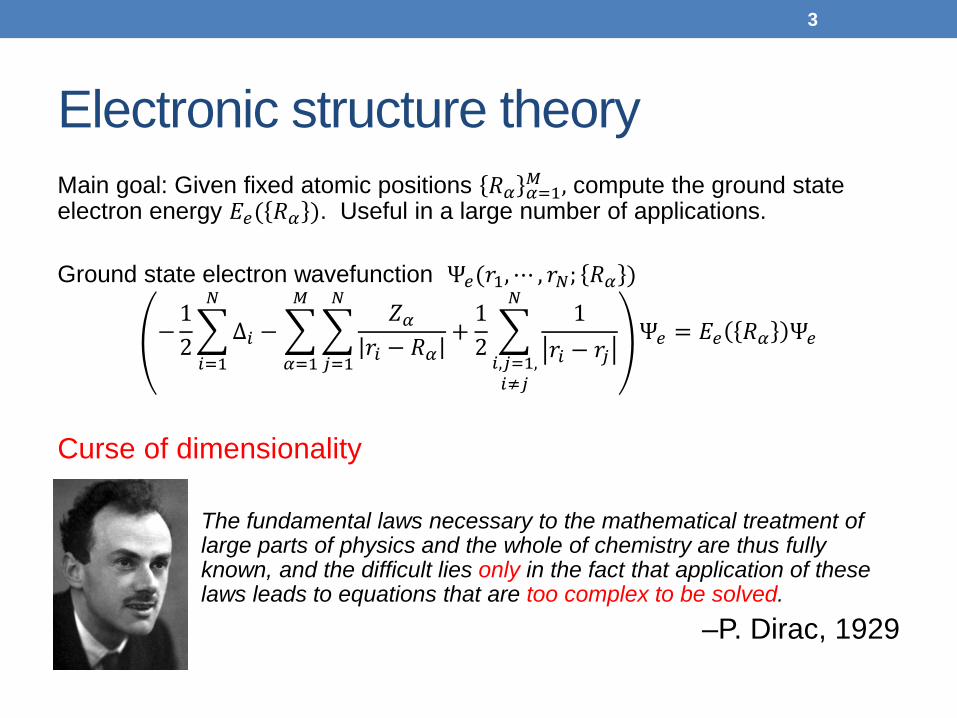
Electronic structure theory Main goal: Given fixed atomic positions 𝑅𝛼 𝛼=1

𝑀 , compute the ground state electron energy 𝐸𝑒( 𝑅𝛼 ). Useful in a large number of applications. Ground state electron wavefunction Ψ𝑒(𝑟1,⋯ , 𝑟𝑁; 𝑅𝛼 )

−12�Δ𝑖 −��

𝑍𝛼𝑟𝑖 − 𝑅𝛼

+12�

1𝑟𝑖 − 𝑟𝑗

𝑁

𝑖,𝑗=1,𝑖≠𝑗

𝑁

𝑗=1

𝑀

𝛼=1

𝑁

𝑖=1

Ψ𝑒 = 𝐸𝑒 𝑅𝛼 Ψ𝑒

Curse of dimensionality

The fundamental laws necessary to the mathematical treatment of large parts of physics and the whole of chemistry are thus fully known, and the difficult lies only in the fact that application of these laws leads to equations that are too complex to be solved.

–P. Dirac, 1929

3

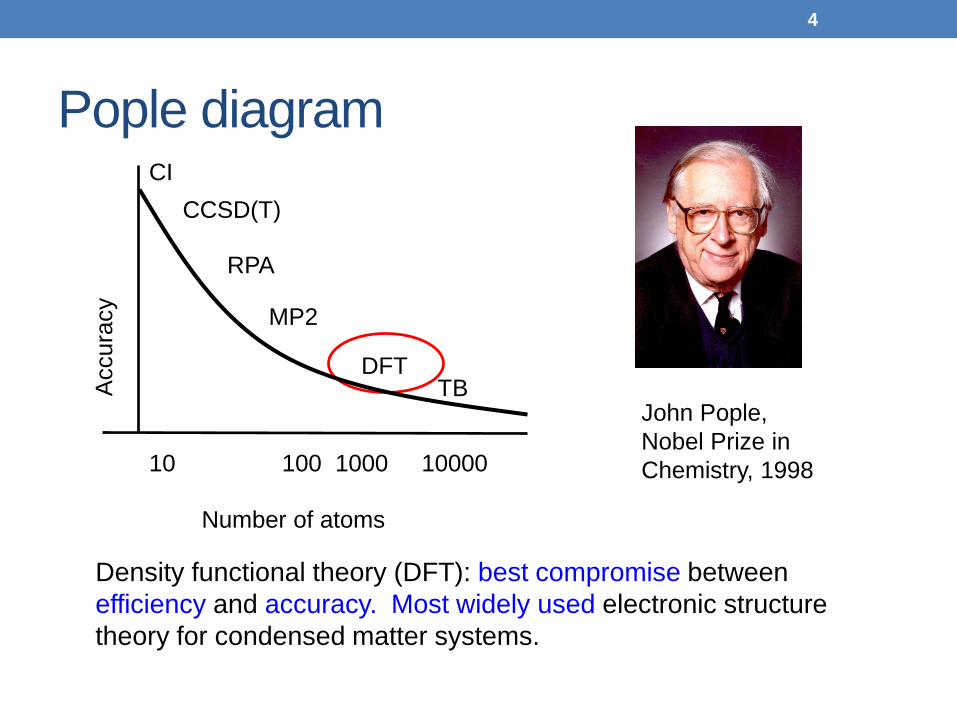
Pople diagram

John Pople, Nobel Prize in Chemistry, 1998

Acc

urac

y

CI CCSD(T)

RPA

MP2

DFT TB

10 100 1000 10000

Number of atoms

Density functional theory (DFT): best compromise between efficiency and accuracy. Most widely used electronic structure theory for condensed matter systems.

4

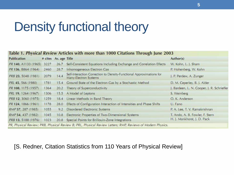
Density functional theory [S. Redner, Citation Statistics from 110 Years of Physical Review]

5

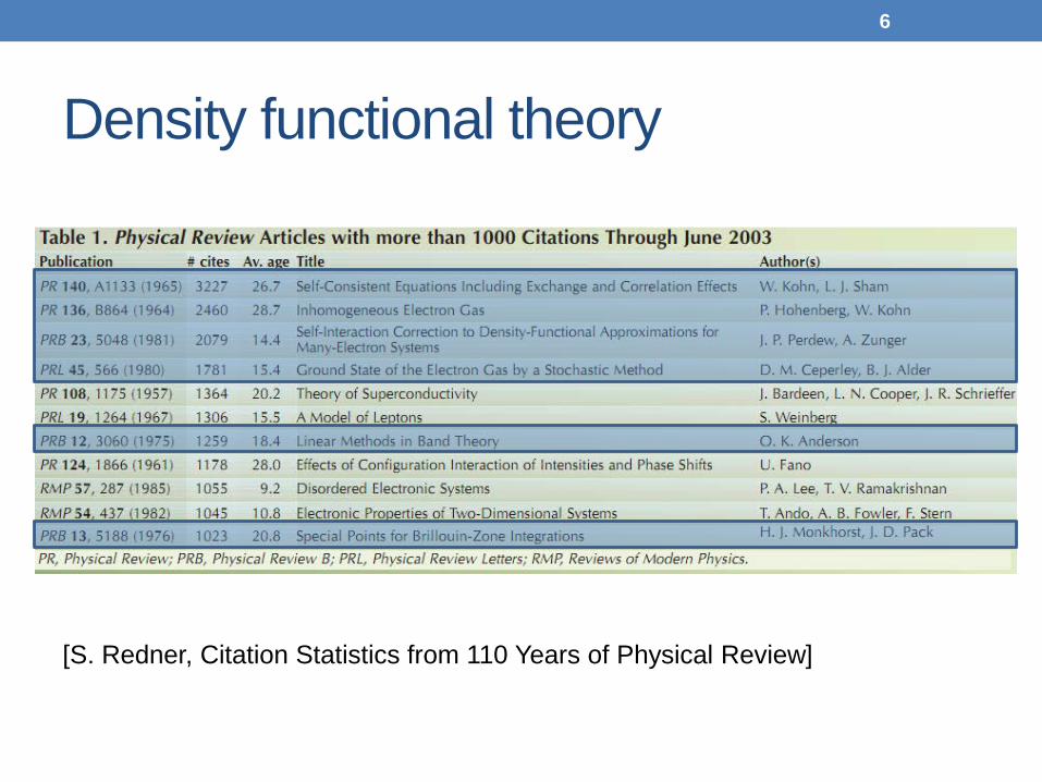
Density functional theory [S. Redner, Citation Statistics from 110 Years of Physical Review]

6

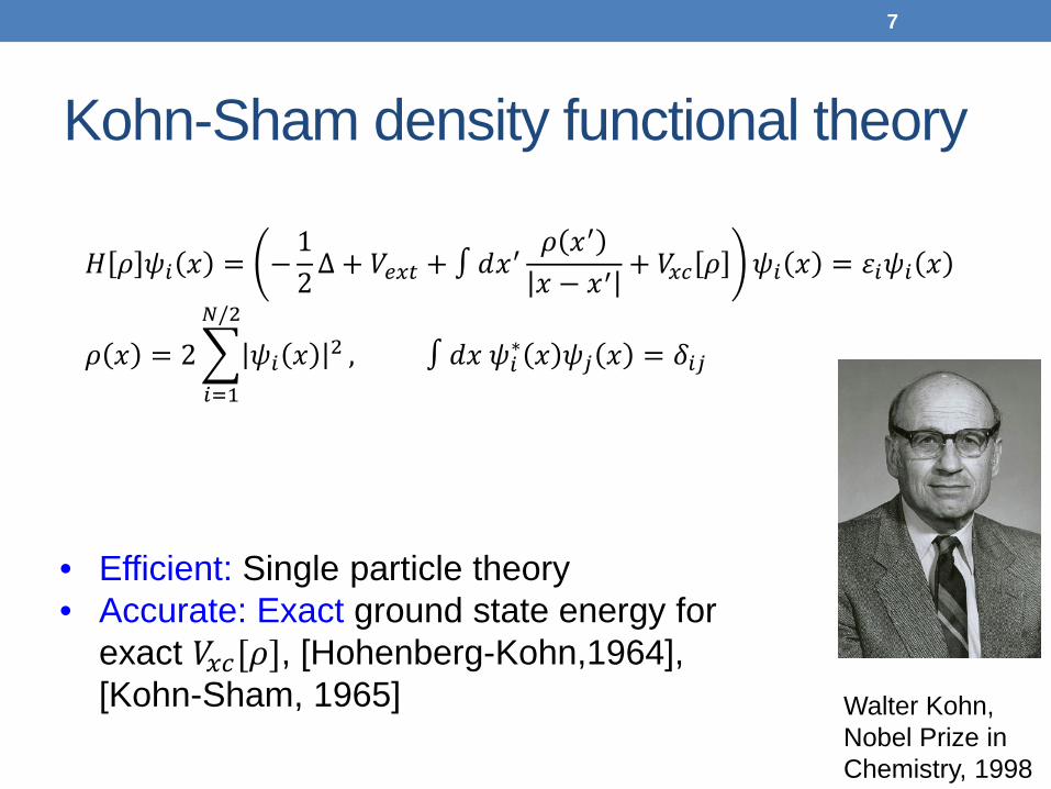
Kohn-Sham density functional theory

• Efficient: Single particle theory • Accurate: Exact ground state energy for

exact 𝑉𝑥𝑥[𝜌], [Hohenberg-Kohn,1964], [Kohn-Sham, 1965]

7

𝐻 𝜌 𝜓𝑖 𝑥 = −12Δ + 𝑉𝑒𝑥𝑒 + ∫ 𝑑𝑥′

𝜌 𝑥′

𝑥 − 𝑥′+ 𝑉𝑥𝑥 𝜌 𝜓𝑖 𝑥 = 𝜀𝑖𝜓𝑖 𝑥

𝜌 𝑥 = 2� 𝜓𝑖 𝑥 2𝑁/2

𝑖=1

, ∫ 𝑑𝑥 𝜓𝑖∗ 𝑥 𝜓𝑗 𝑥 = 𝛿𝑖𝑗

Walter Kohn, Nobel Prize in Chemistry, 1998

Self Consistent Field Iteration

8

𝐻[𝜌𝑖𝑖] 𝜌𝑖𝑖

𝜌𝑜𝑜𝑒

Discretization

Evaluation Iteration

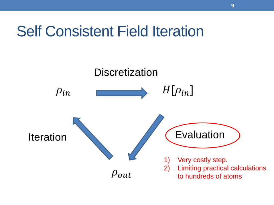
Self Consistent Field Iteration

9

𝐻[𝜌𝑖𝑖] 𝜌𝑖𝑖

𝜌𝑜𝑜𝑒

Discretization

Evaluation Iteration

1) Very costly step. 2) Limiting practical calculations

to hundreds of atoms

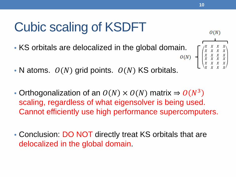
Cubic scaling of KSDFT

10

• KS orbitals are delocalized in the global domain.

• N atoms. 𝑂(𝑁) grid points. 𝑂(𝑁) KS orbitals. • Orthogonalization of an 𝑂 𝑁 × 𝑂(𝑁) matrix ⇒ 𝑂 𝑁3

scaling, regardless of what eigensolver is being used. Cannot efficiently use high performance supercomputers.

• Conclusion: DO NOT directly treat KS orbitals that are

delocalized in the global domain.

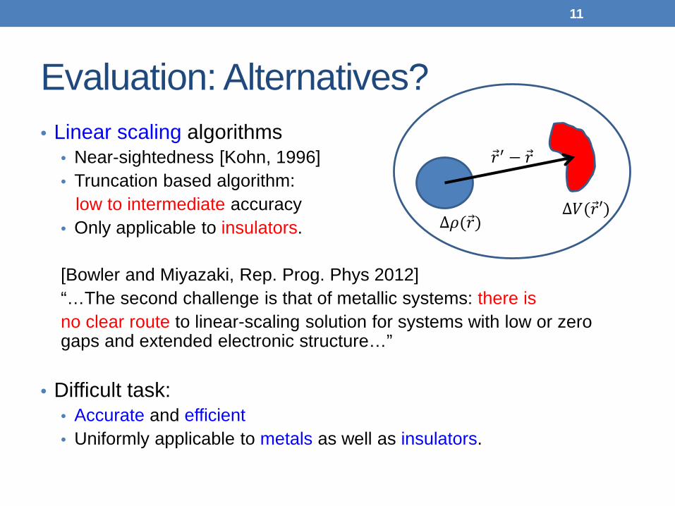
Evaluation: Alternatives? • Linear scaling algorithms

• Near-sightedness [Kohn, 1996] • Truncation based algorithm: low to intermediate accuracy • Only applicable to insulators.

[Bowler and Miyazaki, Rep. Prog. Phys 2012] “…The second challenge is that of metallic systems: there is no clear route to linear-scaling solution for systems with low or zero gaps and extended electronic structure…”

• Difficult task:

• Accurate and efficient • Uniformly applicable to metals as well as insulators.

11

Δ𝑉(𝑟′) Δ𝜌(𝑟)

𝑟′ − 𝑟

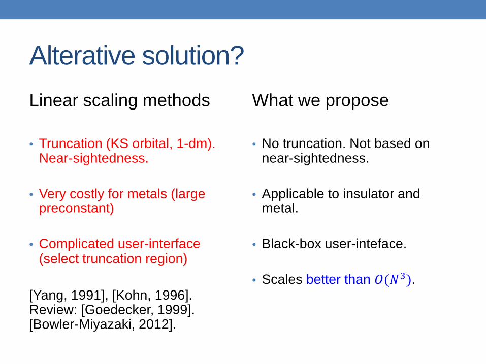
Alterative solution? Linear scaling methods

• Truncation (KS orbital, 1-dm). Near-sightedness.

• Very costly for metals (large

preconstant)

• Complicated user-interface (select truncation region)

[Yang, 1991], [Kohn, 1996]. Review: [Goedecker, 1999]. [Bowler-Miyazaki, 2012].

What we propose • No truncation. Not based on

near-sightedness.

• Applicable to insulator and metal.

• Black-box user-inteface. • Scales better than 𝑂(𝑁3).

Outline

PEXSI: Pole EXpansion Selected Inversion

• Pole Expansion • Selected Inversion • How it works in practice

13

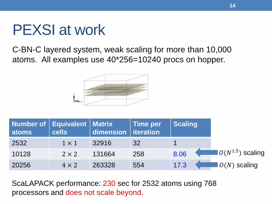
PEXSI at work

14

C-BN-C layered system, weak scaling for more than 10,000 atoms. All examples use 40*256=10240 procs on hopper.

Number of atoms

Equivalent cells

Matrix dimension

Time per iteration

Scaling

2532 1 × 1 32916 32 1 10128 2 × 2 131664 258 8.06 20256 4 × 2 263328 554 17.3

𝑂(𝑁1.5) scaling

𝑂(𝑁) scaling

ScaLAPACK performance: 230 sec for 2532 atoms using 768 processors and does not scale beyond.

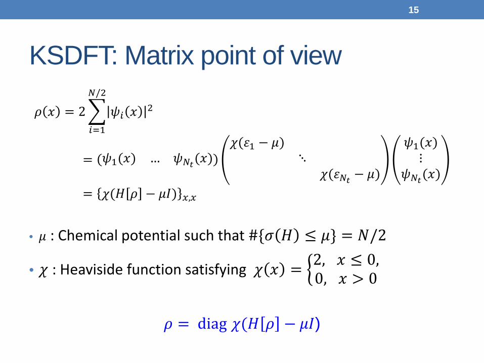
KSDFT: Matrix point of view

𝜌 𝑥 = 2� 𝜓𝑖 𝑥 2𝑁/2

𝑖=1

= 𝜓1(𝑥) … 𝜓𝑁𝑡(𝑥)𝜒(𝜀1 − 𝜇)

⋱ 𝜒(𝜀𝑁𝑡 − 𝜇)

𝜓1(𝑥)⋮

𝜓𝑁𝑡(𝑥)= 𝜒(𝐻 𝜌 − 𝜇𝜇) 𝑥,𝑥

• 𝜇 : Chemical potential such that #{𝜎 𝐻 ≤ 𝜇} = 𝑁/2

• 𝜒 : Heaviside function satisfying 𝜒 𝑥 = �2, 𝑥 ≤ 0,0, 𝑥 > 0

𝜌 = diag 𝜒(𝐻 𝜌 − 𝜇𝜇)

15

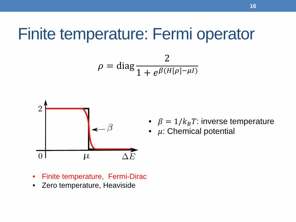
Finite temperature: Fermi operator

𝜌 = diag2

1 + 𝑒𝛽(𝐻[𝜌]−𝜇𝜇)

• 𝛽 = 1/𝑘𝐵𝑇: inverse temperature • 𝜇: Chemical potential

• Finite temperature, Fermi-Dirac • Zero temperature, Heaviside

16

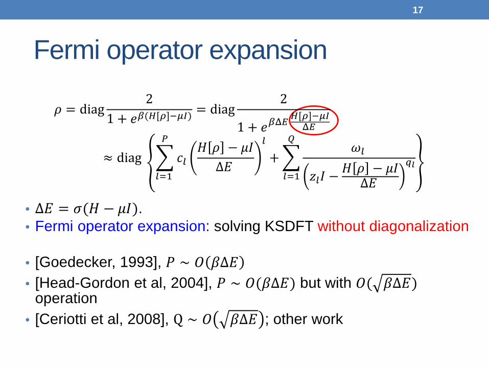
Fermi operator expansion

• Δ𝐸 = 𝜎(𝐻 − 𝜇𝜇). • Fermi operator expansion: solving KSDFT without diagonalization

• [Goedecker, 1993], 𝑃 ∼ 𝑂 𝛽Δ𝐸 • [Head-Gordon et al, 2004], 𝑃 ∼ 𝑂(𝛽Δ𝐸) but with 𝑂( 𝛽Δ𝐸)

operation • [Ceriotti et al, 2008], Q ∼ 𝑂 𝛽Δ𝐸 ; other work

𝜌 = diag2

1 + 𝑒𝛽(𝐻[𝜌]−𝜇𝜇) = diag2

1 + 𝑒𝛽Δ𝐸 𝐻[𝜌]−𝜇𝜇Δ𝐸

≈ diag �𝑐𝑙

𝑃

𝑙=1

𝐻 𝜌 − 𝜇𝜇Δ𝐸

𝑙

+ �𝜔𝑙

𝑧𝑙𝜇 −𝐻 𝜌 − 𝜇𝜇

Δ𝐸 𝑞𝑙

𝑄

𝑙=1

17

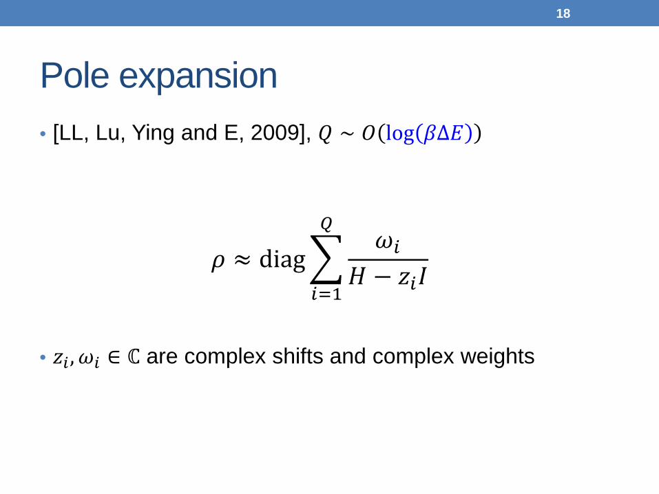
Pole expansion • [LL, Lu, Ying and E, 2009], 𝑄 ∼ 𝑂 log 𝛽Δ𝐸

𝜌 ≈ diag�𝜔𝑖

𝐻 − 𝑧𝑖𝜇

𝑄

𝑖=1

• 𝑧𝑖 ,𝜔𝑖 ∈ ℂ are complex shifts and complex weights

18

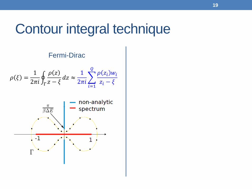
Contour integral technique

Fermi-Dirac

𝜌 𝜉 =12𝜋𝜋

�𝜌 𝑧𝑧 − 𝜉

𝑑𝑧 ≈12𝜋𝜋

�𝜌 𝑧𝑖 𝑤𝑖𝑧𝑖 − 𝜉

𝑄

𝑖=1Γ

19

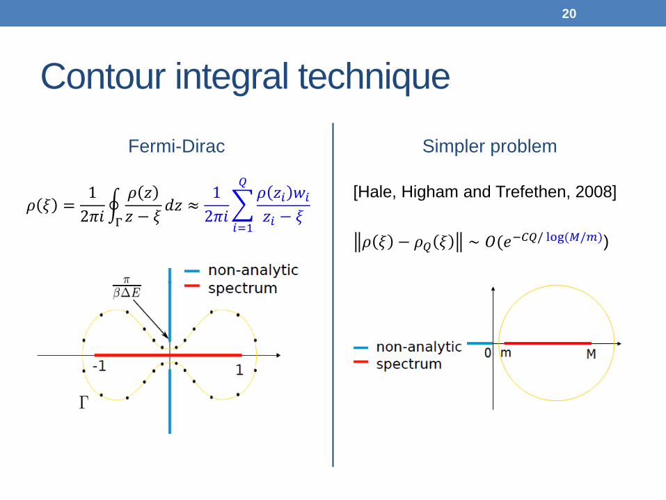
Contour integral technique

Fermi-Dirac

𝜌 𝜉 =12𝜋𝜋

�𝜌 𝑧𝑧 − 𝜉

𝑑𝑧 ≈12𝜋𝜋

�𝜌 𝑧𝑖 𝑤𝑖𝑧𝑖 − 𝜉

𝑄

𝑖=1Γ

Simpler problem

[Hale, Higham and Trefethen, 2008] 𝜌 𝜉 − 𝜌𝑄 𝜉 ∼ 𝑂(𝑒−𝐶𝑄/ log(𝑀/𝑚))

20

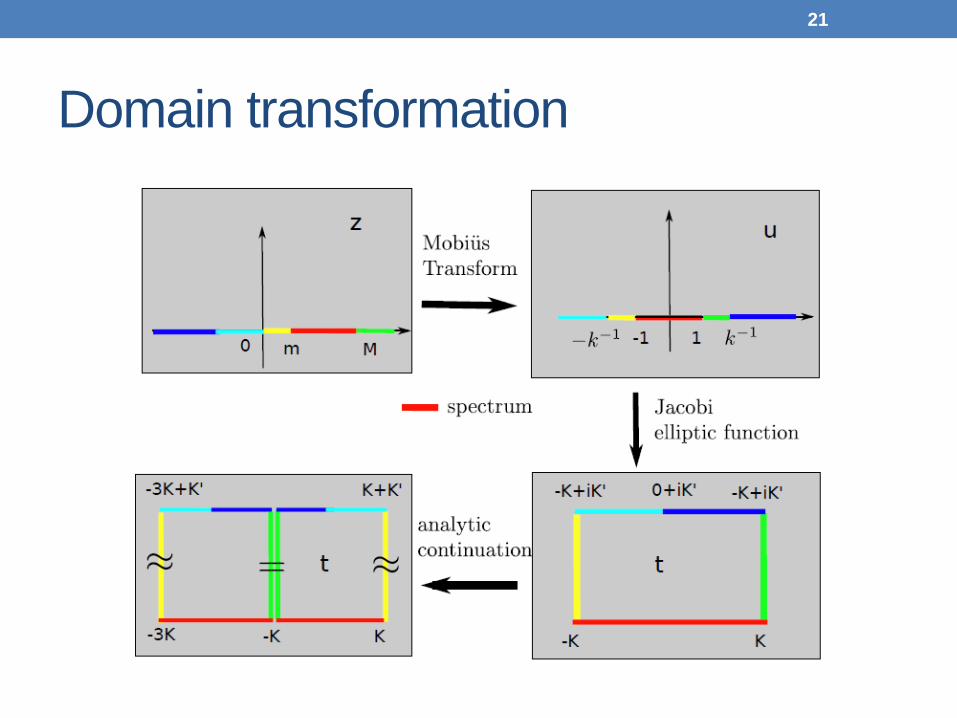
Domain transformation

21

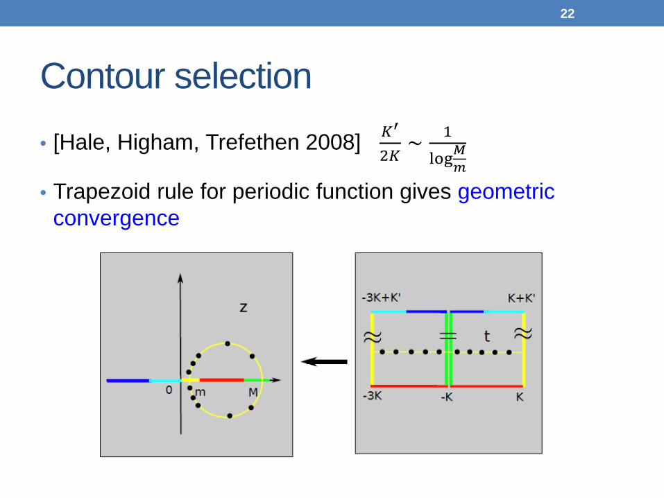
Contour selection • [Hale, Higham, Trefethen 2008] 𝐾

′

2𝐾∼ 1

log𝑀𝑚

• Trapezoid rule for periodic function gives geometric convergence

22

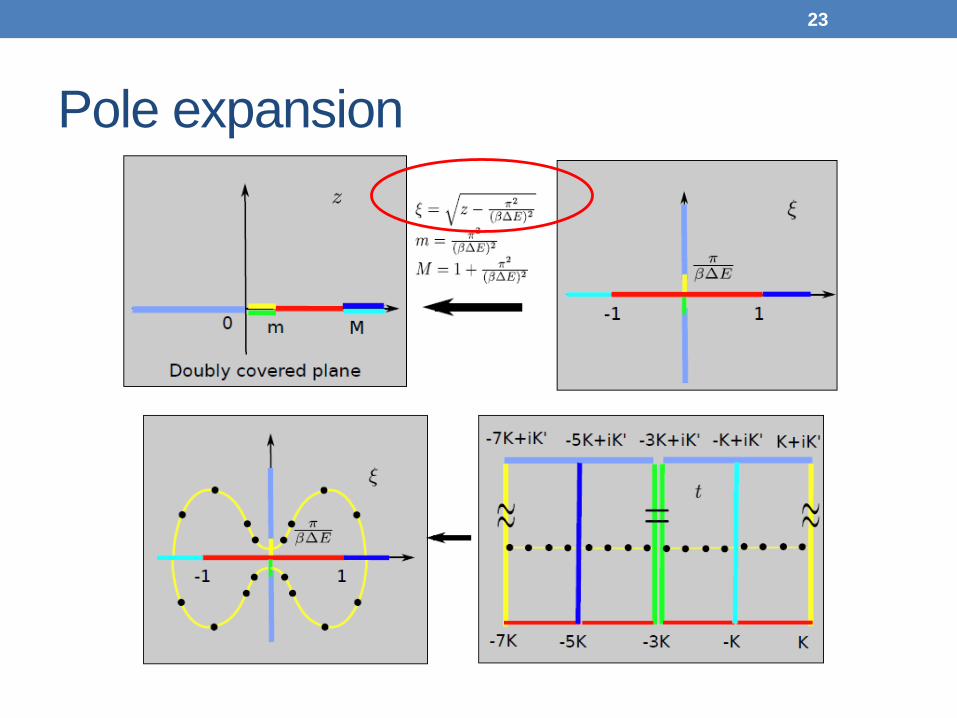
Pole expansion

23

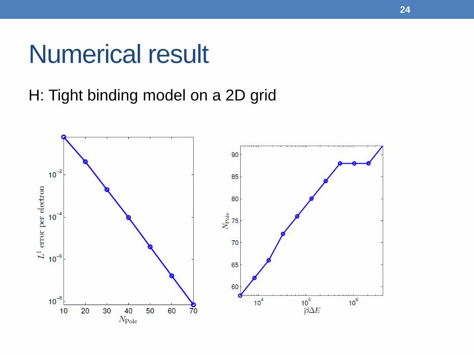
Numerical result H: Tight binding model on a 2D grid

24

Outline

PEXSI: Pole EXpansion Selected Inversion

• Pole Expansion • Selected Inversion • How it works in practice

25

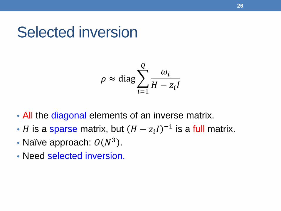
Selected inversion

𝜌 ≈ diag�𝜔𝑖

𝐻 − 𝑧𝑖𝜇

𝑄

𝑖=1

• All the diagonal elements of an inverse matrix. • 𝐻 is a sparse matrix, but 𝐻 − 𝑧𝑖𝜇 −1 is a full matrix. • Naïve approach: 𝑂 𝑁3 . • Need selected inversion.

26

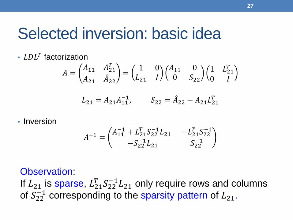
Selected inversion: basic idea • 𝐿𝐿𝐿𝑇 factorization

𝐴 =𝐴11 𝐴21𝑇

𝐴21 �̂�22= 1 0

𝐿21 𝜇𝐴11 0

0 𝑆221 𝐿21𝑇0 𝜇

𝐿21 = 𝐴21𝐴11−1, 𝑆22 = �̂�22 − 𝐴21𝐿21𝑇

• Inversion

𝐴−1 = 𝐴11−1 + 𝐿21𝑇 𝑆22−1𝐿21 −𝐿21𝑇 𝑆22−1

−𝑆22−1𝐿21 𝑆22−1

27

Observation: If 𝐿21 is sparse, 𝐿21𝑇 𝑆22−1𝐿21 only require rows and columns of 𝑆22−1 corresponding to the sparsity pattern of 𝐿21.

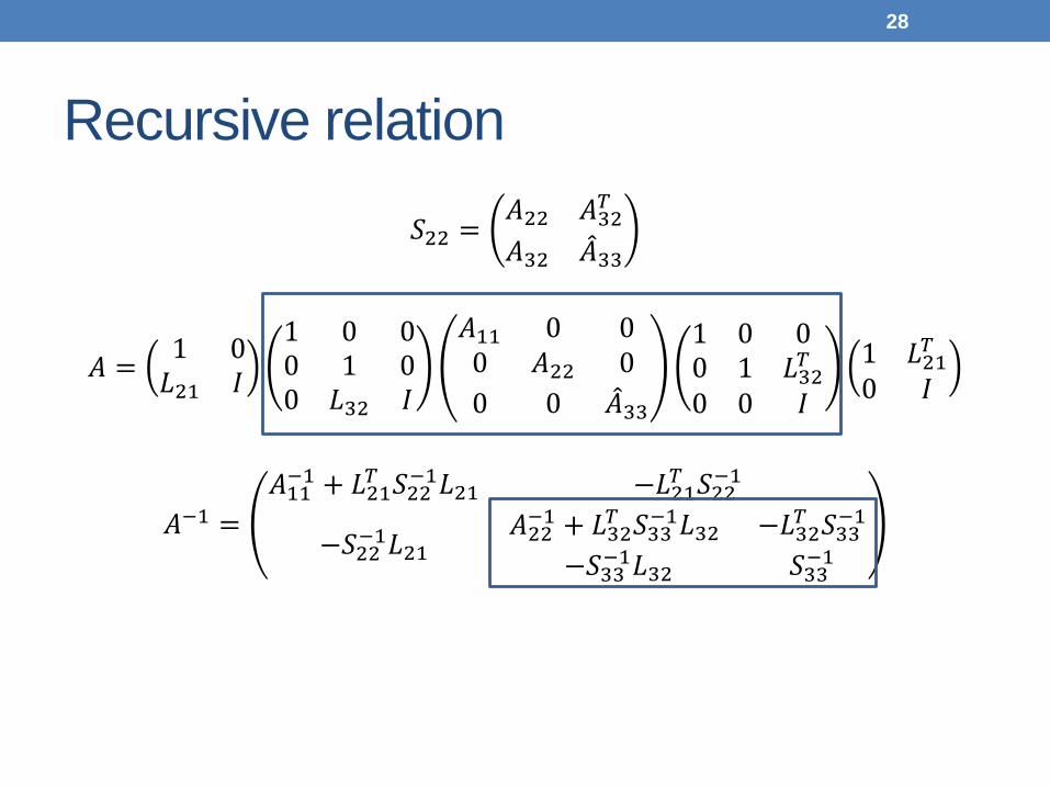
Recursive relation

𝑆22 =𝐴22 𝐴32𝑇

𝐴32 �̂�33

𝐴 = 1 0𝐿21 𝜇

1 0 00 1 00 𝐿32 𝜇

𝐴11 0 00 𝐴22 00 0 �̂�33

1 0 00 1 𝐿32𝑇0 0 𝜇

1 𝐿21𝑇0 𝜇

𝐴−1 =𝐴11−1 + 𝐿21𝑇 𝑆22−1𝐿21 −𝐿21𝑇 𝑆22−1

−𝑆22−1𝐿21𝐴22−1 + 𝐿32𝑇 𝑆33−1𝐿32 −𝐿32𝑇 𝑆33−1

−𝑆33−1𝐿32 𝑆33−1

28

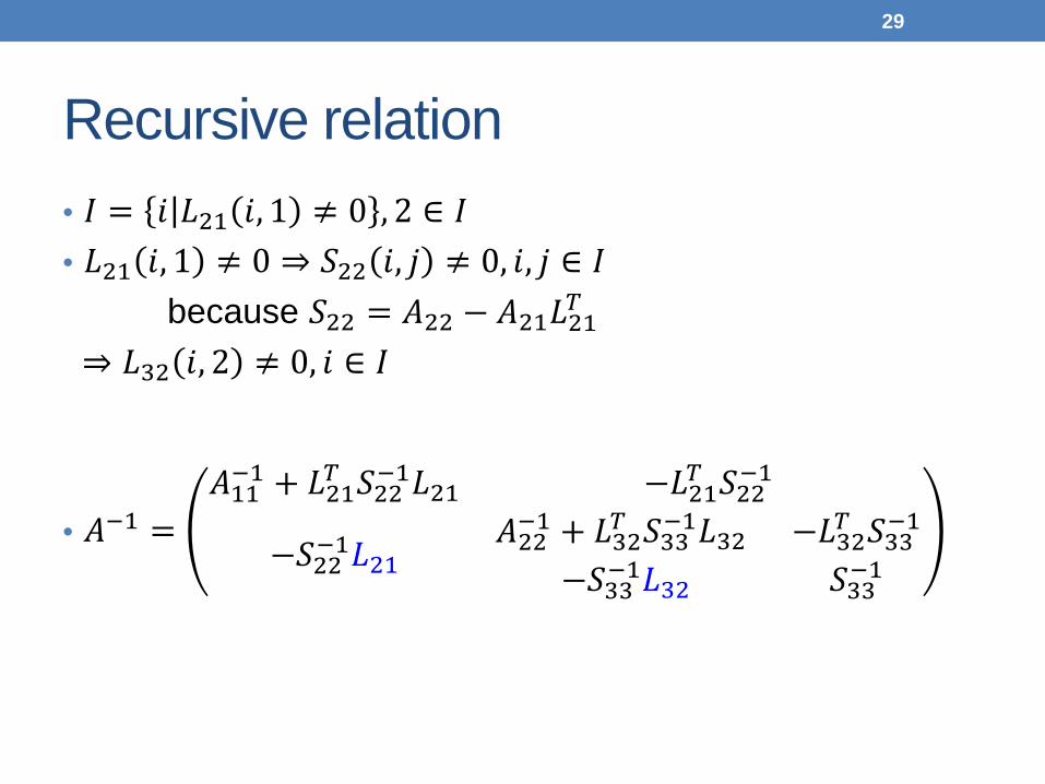
Recursive relation • 𝜇 = 𝜋 𝐿21 𝜋, 1 ≠ 0 , 2 ∈ 𝜇 • 𝐿21 𝜋, 1 ≠ 0 ⇒ 𝑆22 𝜋, 𝑗 ≠ 0, 𝜋, 𝑗 ∈ 𝜇 because 𝑆22 = 𝐴22 − 𝐴21𝐿21𝑇 ⇒ 𝐿32 𝜋, 2 ≠ 0, 𝜋 ∈ 𝜇

• 𝐴−1 =𝐴11−1 + 𝐿21𝑇 𝑆22−1𝐿21 −𝐿21𝑇 𝑆22−1

−𝑆22−1𝐿21𝐴22−1 + 𝐿32𝑇 𝑆33−1𝐿32 −𝐿32𝑇 𝑆33−1

−𝑆33−1𝐿32 𝑆33−1

29

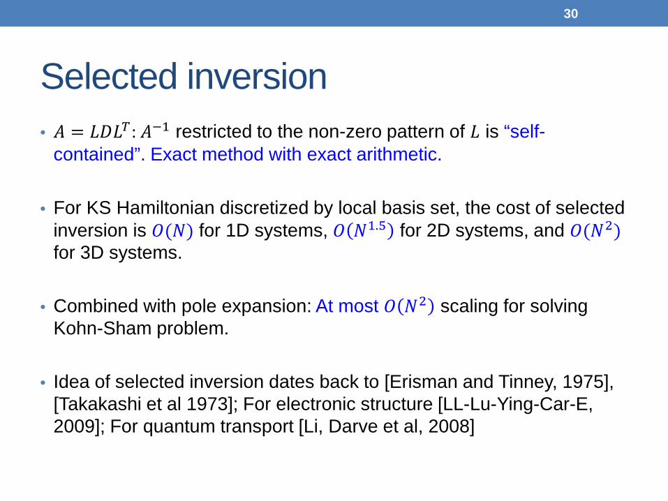
Selected inversion • 𝐴 = 𝐿𝐿𝐿𝑇: 𝐴−1 restricted to the non-zero pattern of 𝐿 is “self-

contained”. Exact method with exact arithmetic.

• For KS Hamiltonian discretized by local basis set, the cost of selected inversion is 𝑂(𝑁) for 1D systems, 𝑂 𝑁1.5 for 2D systems, and 𝑂(𝑁2) for 3D systems.

• Combined with pole expansion: At most 𝑂 𝑁2 scaling for solving Kohn-Sham problem.

• Idea of selected inversion dates back to [Erisman and Tinney, 1975],

[Takakashi et al 1973]; For electronic structure [LL-Lu-Ying-Car-E, 2009]; For quantum transport [Li, Darve et al, 2008]

30

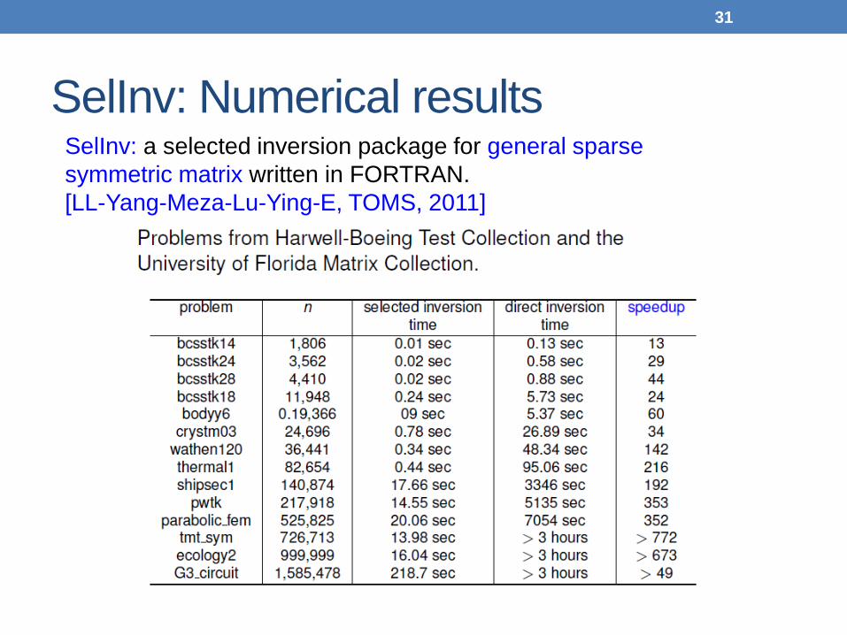
SelInv: Numerical results SelInv: a selected inversion package for general sparse symmetric matrix written in FORTRAN. [LL-Yang-Meza-Lu-Ying-E, TOMS, 2011]

31

Outline

PEXSI: Pole EXpansion Selected Inversion

• Pole Expansion • Selected Inversion • How it works in practice

32

Force

33

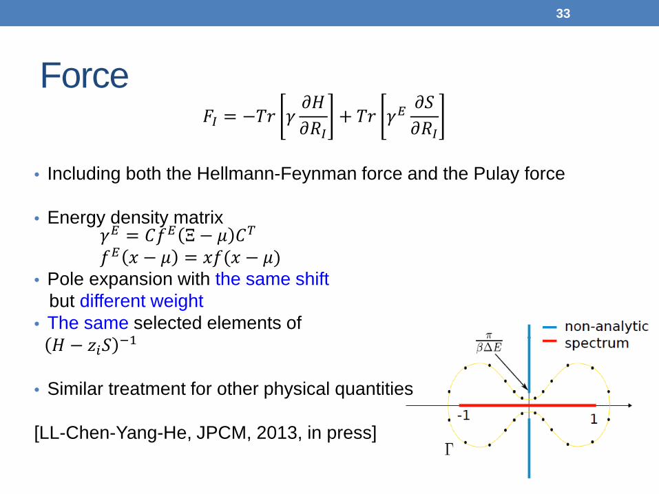
𝐹𝜇 = −𝑇𝑟 𝛾𝜕𝐻𝜕𝑅𝜇

+ 𝑇𝑟 𝛾𝐸𝜕𝑆𝜕𝑅𝜇

• Including both the Hellmann-Feynman force and the Pulay force • Energy density matrix

𝛾𝐸 = 𝐶𝑓𝐸 Ξ − 𝜇 𝐶𝑇 𝑓𝐸 𝑥 − 𝜇 = 𝑥𝑓(𝑥 − 𝜇) • Pole expansion with the same shift but different weight • The same selected elements of 𝐻 − 𝑧𝑖𝑆 −1

• Similar treatment for other physical quantities

[LL-Chen-Yang-He, JPCM, 2013, in press]

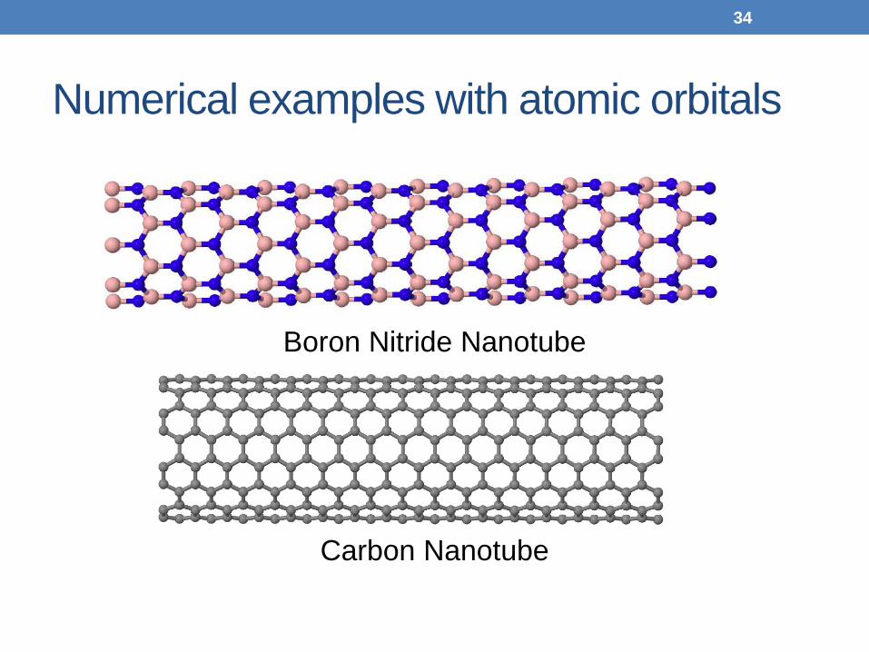
Numerical examples with atomic orbitals

Boron Nitride Nanotube

Carbon Nanotube

34

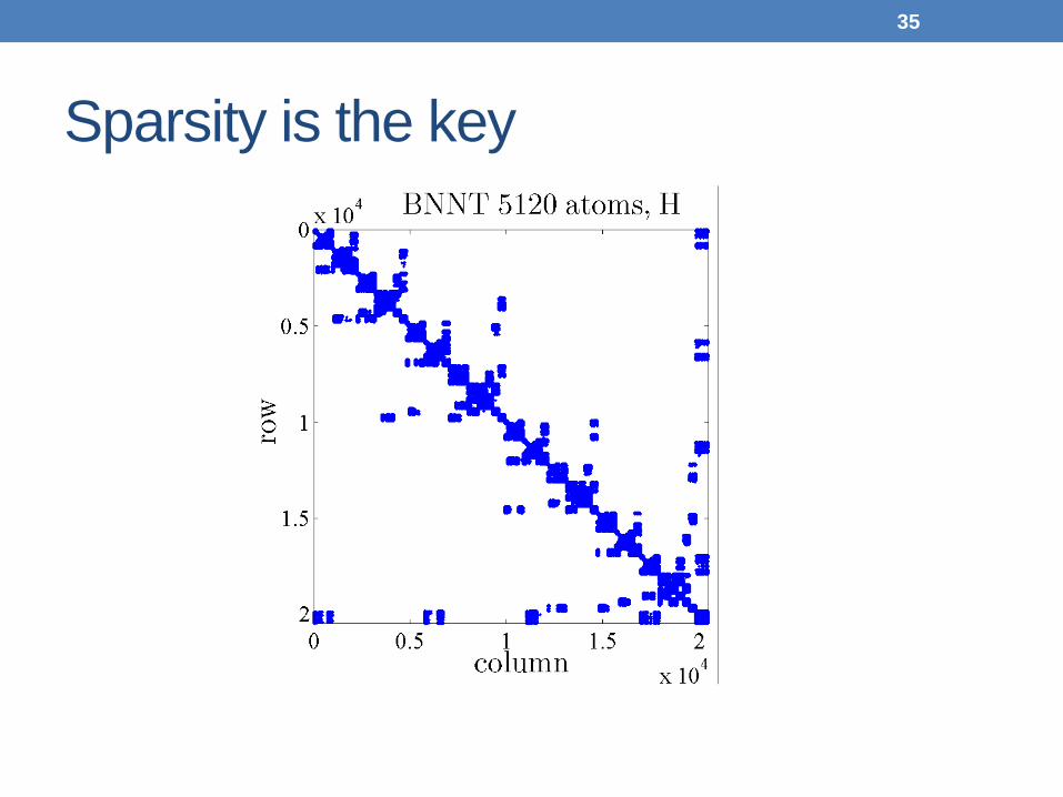
Sparsity is the key

35

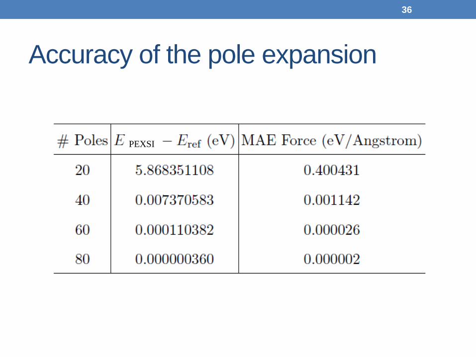
Accuracy of the pole expansion

36

PEXSI

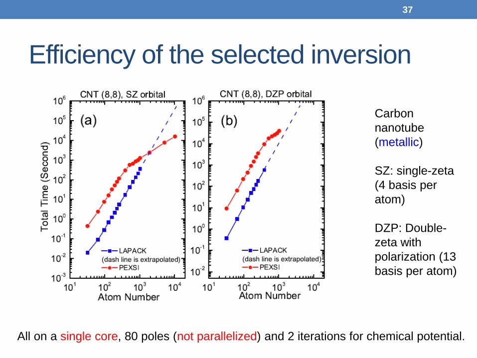
Efficiency of the selected inversion

37

Carbon

nanotube (metallic) SZ: single-zeta (4 basis per atom) DZP: Double-zeta with polarization (13 basis per atom)

All on a single core, 80 poles (not parallelized) and 2 iterations for chemical potential.

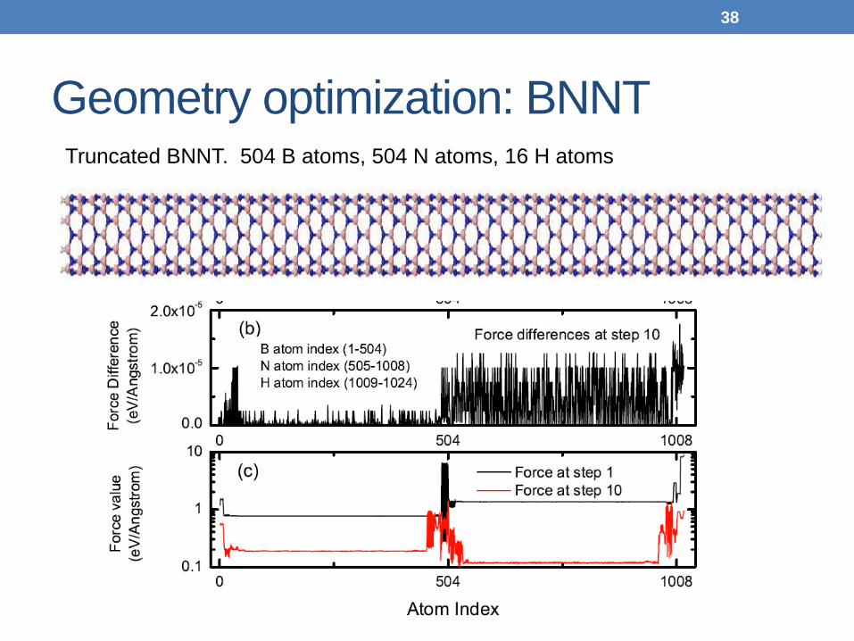
Geometry optimization: BNNT

38

Truncated BNNT. 504 B atoms, 504 N atoms, 16 H atoms

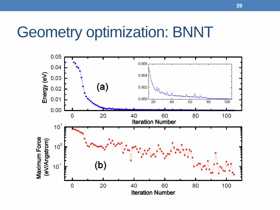
Geometry optimization: BNNT

39

PEXSI in parallel • Distributed memory parallel selected inversion for general

matrix (factorization is based on SuperLU_DIST), preliminary version scalable to 64 ~ 256 procs. More efficient version under progress (ongoing work with Mathias Jacquelin and Chao Yang)

• Pole expansion parallelized. With 40 poles used in practice, PEXSI can scale to 256*40~10,000 procs.

• C++ implementation. Nearly black-box interface, being integrated to SIESTA (ongoing work with Alberto Garcia, Georg Huhs and Chao Yang)

40

PEXSI in parallel

41

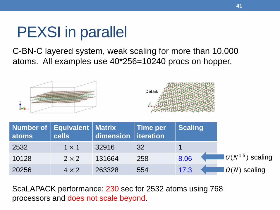
C-BN-C layered system, weak scaling for more than 10,000 atoms. All examples use 40*256=10240 procs on hopper.

Number of atoms

Equivalent cells

Matrix dimension

Time per iteration

Scaling

2532 1 × 1 32916 32 1 10128 2 × 2 131664 258 8.06 20256 4 × 2 263328 554 17.3

𝑂(𝑁1.5) scaling

𝑂(𝑁) scaling

ScaLAPACK performance: 230 sec for 2532 atoms using 768 processors and does not scale beyond.

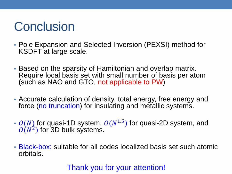
Conclusion • Pole Expansion and Selected Inversion (PEXSI) method for

KSDFT at large scale.

• Based on the sparsity of Hamiltonian and overlap matrix. Require local basis set with small number of basis per atom (such as NAO and GTO, not applicable to PW)

• Accurate calculation of density, total energy, free energy and force (no truncation) for insulating and metallic systems.

• 𝑂(𝑁) for quasi-1D system, 𝑂(𝑁1.5) for quasi-2D system, and 𝑂(𝑁2) for 3D bulk systems.

• Black-box: suitable for all codes localized basis set such atomic orbitals.

Thank you for your attention!