Fast algorithms for maximizing submodular functions

Ashwinkumar Badanidiyuru ∗ Jan Vondrak †

October 9, 2013

Abstract

There has been much progress recently on improvedapproximations for problems involving submodular ob-jective functions, and many interesting techniques havebeen developed. However, the resulting algorithms areoften slow and impractical. In this paper we developalgorithms that match the best known approximationguarantees, but with significantly improved runningtimes, for maximizing a monotone submodular functionf : 2[n] → R+ subject to various constraints. As in pre-vious work, we measure the number of oracle calls tothe objective function which is the dominating term inthe running time.

Our first result is a simple algorithm that gives a(1− 1/e− ε)-approximation for a cardinality constraintusing O(nε log n

ε ) queries, and a 1/(p + 2` + 1 + ε)-approximation for the intersection of a p-system and `knapsack (linear) constraints using O( nε2 log2 n

ε ) queries.This is the first approximation for a p-system combinedwith linear constraints. (We also show that the factor ofp cannot be improved for maximizing over a p-system.)The main idea behind these algorithms serves as abuilding block in our more sophisticated algorithms.

Our main result is a new variant of the continu-ous greedy algorithm, which interpolates between theclassical greedy algorithm and a truly continuous algo-rithm. We show how this algorithm can be implementedfor matroid and knapsack constraints using O(n2) ora-cle calls to the objective function. (Previous variantsand alternative techniques were known to use at least

O(n4) oracle calls.) This leads to an O(n2

ε4 log2 nε )-time

(1 − 1/e − ε)-approximation for a matroid constraint.For a knapsack constraint, we develop a more involved(1−1/e− ε)-approximation algorithm that runs in timeO(n2( 1

ε log n)poly(1/ε)).

∗Department of Computer Science, Cornell University. Email:

ashwinkumarbv@gmail.com. Parts of this research have been

done while A. Badanidiyuru was a research intern at IBM Al-maden Research Center. A. Badanidiyuru was partially supported

by NSF grant AF-0910940 and NSF grant IIS-0905467.†IBM Almaden Research Center, San Jose, CA. E-mail: jvon-

drak@us.ibm.com

1 Introduction

Optimization problems involving maximization of a sub-modular objective function have attracted a lot of at-tention recently. This interest has been driven by sev-eral kinds of applications in which submodular objectivefunctions arise naturally. Let us mention welfare maxi-mization in combinatorial auctions, where the objectivefunction captures the notion of utility function with di-minishing returns [27, 4, 6, 8, 33]. A second applicationarises in the area of social networks, where the functionscharacterizing the influence of a subset of nodes turn outto be submodular [17, 18]. Another one is the problemof intelligent gathering of information, where sensorsshould be placed in order to maximize the informationthat can be collected from them [14, 21, 28, 23, 20, 22].In this case, submodularity arises due to the fact thatthe entropy of a collection of random variables is a sub-modular function. Submodular functions also provide aunifying framework which captures optimization prob-lems that have been studied earlier, such that Min Cut,Max Cut, Multiway Cut, Max k-Cover, the GeneralizedAssignment Problem, the Separable Assignment Prob-lem, etc.

In these settings, the goal is to optimize a submod-ular function subject to certain constraints. In fact,in many cases the constraints at hand are quite sim-ple, such as cardinality (maxf(S) : |S| ≤ k), or apartition matroid (maxf(S) : |S ∩ Pi| ≤ 1∀i, wherePi are disjoint sets). In some applications, combina-tions of several of such constraints can arise, such as acombination of several matroid constraints and knap-sack constraints (

∑j∈S cj ≤ 1). For a long time, the

only work in this area had been a sequence of papers byFisher, Nemhauser and Wolsey [30, 12, 29]. The mainresult of this work is that the greedy algorithm providesrelatively good approximation for these problems: inparticular, a (1− 1/e)-approximation for maximizing amonotone submodular functions subject to a cardinalityconstraint, and a (k + 1)-approximation for maximiza-tion of a monotone submodular function subject to kmatroid constraints. An additional virtue of the greedyalgorithm is that it is very simple and fast (quadraticrunning time in the straightforward implementation).

Recently, there has been a wave of effort to im-prove this result and extend it to more general scenar-ios. A (1 − 1/e)-approximation was given for the caseof 1 knapsack constraint [32]. For the case of 1 ma-troid constraint, which is relevant particularly in thesetting of combinatorial auctions, an optimal (1− 1/e)-approximation was found in [33, 2]. For any con-stant number of knapsack constraints, a (1 − 1/e − ε)-approximation was given in [24]. For k matroid con-straints, the (k + 1)-approximation has been improvedto k + ε for any fixed ε > 0 [26]. Extensions and gener-alizations to nonmonotone submodular functions havebeen developed in [7, 25, 34, 26, 16, 13, 9, 10, 3, 1].

A common trait of these algorithms is that they pro-vide good approximations, often close to optimal, buttheir running time is typically far from practical. (Withtwo exceptions: [16] gives a fast algorithm for maximiz-ing a submodular function subject to a p-system, gener-alizing the monotone case from [12]; [1] gives an optimal1/2-approximation for maximizing a submodular func-tion without any constraints, and runs in linear time.)Let us mention some other recent advances and theirlimitations in terms of running time:• The notion of multilinear relaxation has been used toachieve an optimal (1−1/e)-approximation for submod-ular maximization subject to a matroid constraint [2],as well as improved approximations for more generalvariants [24, 34, 9, 13, 3]. Nevertheless, the continuousgreedy algorithm, the primary algorithmic tool here, hasbeen quoted to run in time Θ(n8) [11].• Recently, an alternative way to derive a (1 − 1/e)-approximation for 1 matroid constraint, which does notrequire the multilinear relaxation, was given in [11]. Itgives a (1− 1/e− ε)-approximation in time O(nr4ε−3),where r is the rank of the matroid. The authors showthat the continuous greedy algorithm would have a sim-ilar performance if adapted to give a (1 − 1/e − ε)-approximation.• For combined constraints such as multiple knapsacks,known algorithms rely on enumeration of poly(1/ε)items [24, 3] or a reduction to partition matroids [15],both of which lead to Ω(npoly(1/ε)) running times. Thedependence in the exponent is bad enough that thesealgorithms do not seem practical even for ε = 1

2 .Due to these issues, it appears that few of these new

algorithms are fast enough to be applied in practice.In fact, it turns out that even the original greedyalgorithm, which takes O(rn) running time, is too slowfor many applications, and researchers have sought waysto speed up the greedy algorithm as well [28, 23]. Ourgoal in this paper is to remedy this situation and developalgorithms that have both theoretical approximationguarantees, and a more practical running time.

Our results. In the following, n denotes the total num-ber of elements, and r denotes the maximum cardinalityof a feasible solution. We measure the complexity of analgorithm in terms of the number of oracle calls. Wenote that the total running time of our algorithms isnot worse than O(n)× the number of oracle calls, andtypically this would be the actual running time, sincean oracle call involves processing a set of up to n ele-ments. Since the earlier algorithms have been typicallyanalyzed in terms of the number of oracle calls, we usethe same benchmark.Simple thresholding algorithms. First, we present asimple algorithm for the case of a cardinality constraint,which is faster then the classical greedy algorithm andperforms at least as well. A greedy algorithm forselecting r elements uses O(rn) queries. An often usedversion of greedy known as lazy greedy [28, 23] seemsto perform much better in practice. Our algorithmcan be viewed as an alternative implementation of lazygreedy which provides the same approximation and aguaranteed faster running time.

Theorem 1.1. There is a (1− 1/e− ε)-approximationalgorithm for maximizing a monotone submodularfunction subject to a cardinality constraint, usingO(nε log n

ε

)queries.

An extension of this algorithm gives the followingresult for a combination of a p-system and ` linearconstraints.

Theorem 1.2. There is a 1/(p + 2` + 1 + ε)-approximation algorithm for maximizing a monotonesubmodular function subject to an intersection of ap-system and ` knapsack (linear) constraints, usingO( nε2 log2 n

ε ) queries.

To our knowledge, this is the first known approx-imation for the combination of a p-system and knap-sack constraints. It was known that the greedy algo-rithm gives a 1/p-approximation for maximizing a lin-ear function subject to a p-system, and a 1/(p + 1)-approximation for maximizing a monotone submodularfunction subject to a p-system [12]. We also give a sim-ple proof that the factor of p is optimal for p-systems;see Section 7.

Our algorithm uses a combination of two ideas: afast implementation of a greedy algorithm, using a de-creasing value threshold, and a fixed density threshold,to deal with the knapsack constraints. The ideas usedin the above two algorithm also serve as building blocksin the following result.Accelerated continuous greedy algorithm. Ourmain result is a new accelerated continuous greedy

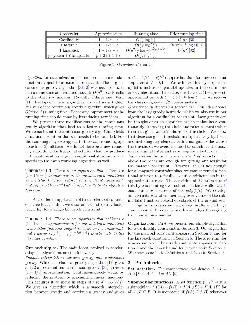
Constraint Approximation Running time Prior running time

Cardinality 1− 1/e− ε O(nε log nε ) O(nr)[30]

1 matroid 1− 1/e− ε O( rnε4 log2 rε ) O(nr3ε−3 log r)[11]

1 knapsack 1− 1/e− ε O(n2( 1ε log n

ε )poly(1/ε)) O(n5)[32]

p-system + ` knapsacks p+ 2`+ 1 + ε O( nε2 log2 nε ) −−−

Figure 1: Overview of results.

algorithm for maximization of a monotone submodularfunction subject to a matroid constraint. The originalcontinuous greedy algorithm [33, 2] was not optimizedfor running time and required roughly O(n8) oracle callsto the objective function. Recently, Filmus and Ward[11] developed a new algorithm, as well as a tighteranalysis of the continuous greedy algorithm, which givesO(r3nε−3) running time. Hence any improvement to therunning time should come by introducing new ideas.

We present three modifications to the continuousgreedy algorithm that lead to a faster running time.We remark that the continuous greedy algorithm yieldsa fractional solution that still needs to be rounded. Forthe rounding stage we appeal to the swap rounding ap-proach of [3]; although we do not develop a new round-ing algorithm, the fractional solution that we producein the optimization stage has additional structure whichspeeds up the swap rounding algorithm as well.

Theorem 1.3. There is an algorithm that achieves a(1−1/e− ε)-approximation for maximizing a monotonesubmodular function subject to a matroid constraint,and requires O(rnε−4 log2 n) oracle calls to the objectivefunction.

As a different application of the accelerated continu-ous greedy algorithm, we show an asymptotically fasteralgorithm for a single knapsack constraint.

Theorem 1.4. There is an algorithm that achieves a(1−1/e− ε)-approximation for maximizing a monotonesubmodular function subject to a knapsack constraint,and requires O(n2( 1

ε log nε )poly(1/ε)) oracle calls to the

objective function.

Our techniques. The main ideas involved in acceler-ating the algorithms are the following.Smooth interpolation between greedy and continuousgreedy: While the classical greedy algorithm [12] givesa 1/2-approximation, continuous greedy [33] gives a(1 − 1/e)-approximation. Continuous greedy works byreducing the problem to maximizing linear functions.This requires it to move in steps of size δ = O(ε/n).We give an algorithm which is a smooth interpola-tion between greedy and continuous greedy and gives

a (1 − 1/(1 + δ)1/δ)-approximation for any constantstep size δ ∈ (0, 1]. We achieve this by sequentialupdates instead of parallel updates in the continuousgreedy algorithm. This allows us to get a (1− 1/e− ε)-approximation with δ = O(ε). When δ = 1, we recoverthe classical greedy 1/2 approximation.Geometrically decreasing thresholds: This idea comesfrom the lazy greedy heuristic, which we also use in ouralgorithm for a cardinality constraint. Lazy greedy canbe thought of as an algorithm which maintains a con-tinuously decreasing threshold and takes elements whentheir marginal value is above the threshold. We showthat decreasing the threshold multiplicatively by 1− ε,and including any element with a marginal value abovethe threshold, we avoid the need to search for the max-imal marginal value and save roughly a factor of n.Enumeration in value space instead of subsets: Theabove two ideas are enough for getting our result forthe matroid constraint. However, this is not enoughfor a knapsack constraint since we cannot round a frac-tional solution to a feasible solution without loss in theapproximation ratio. The algorithm of [32] takes care ofthis by enumerating over subsets of size 3 while [24, 3]enumerates over subsets of size poly(1/ε). We developan alternate way of enumerating over values of the sub-modular function instead of subsets of the ground set.

Figure 1 shows a summary of our results, including acomparison with previous best known algorithms givingthe same approximation.

Organization. First we present our simple algorithmfor a cardinality constraint in Section 3. Our algorithmfor the matroid constraint appears in Section 4, and forthe knapsack constraint in Section 5. The algorithm fora p-system and ` knapsack contraints appears in Sec-tion 6 and the lower bound for p-systems in Section 7.We state some basic definitions and facts in Section 2.

2 Preliminaries

Set notation. For compactness, we denote A + i =A ∪ i and A− i = A \ i.

Submodular functions. A set function f : 2E → R issubmodular, if f(A) + f(B) ≥ f(A∪B) + f(A∩B) forall A,B ⊆ E. It is monotone, if f(A) ⊆ f(B) whenever

A ⊆ B. In this paper, we consider only nonnegative setfunctions, f : 2E → R+.

Matroids. A matroid is a pair M = (E, I) whereI ⊆ 2E is a collection of independent sets, satisfying:(i) A ⊆ B,B ∈ I ⇒ A ∈ I, and (ii) A,B ∈ I, |A| <|B| ⇒ ∃i ∈ B \A;A+ i ∈ I.

p-systems. For a family I ⊆ 2E and a set S ⊆ E, wecall B a base of S, if B is an inclusion-wise maximalsubset of S such that B ∈ I. A p-system is a familyI ⊆ 2E such that for every S ⊆ E and any two basesB1, B2 of S, |B2| ≤ p|B1|.

It is known that for any p matroids M1 =(E, I1), . . . ,Mp = (E, Ip), the intersection

⋂pi=1 Ii is

a p-system. More generally, p-systems include “p-extendible families”, “p-uniform matchoids” and “p-uniform matroid matching”; see [2, 26] for more details.

Knapsack constraints. By a knapsack constraintK ⊆ 2E , we mean a family of sets defined by a linearconstraint K = I ⊆ E :

∑j∈I cj ≤ 1 for some

collection of weights (cj : j ∈ E). (We can assume thatthe capacity is 1 without loss of generality.) Thus theclassical knapsack problem is max

∑j∈I wj : I ∈ K.

The multilinear extension. For a function f : 2E →R, we define F (x) = E[f(R(x))], where R(x) is arandom set where element i appears independently withprobability xi.

Shorthand notation. We will use the following twoshorthand notation.

• For any S, T ⊆ E let fS(T ) = f(S ∪ T )− f(S).

• Let E1 and E2 be two duplicate copies of groundset E. For any S ⊆ E1∪E2 define contract(S) ⊆ Eas the set which contains e ∈ E iff S contains atleast one copy of e. Then define the extension of themonotone submodular function f : 2E1∪E2 → R+

as ∀S ⊆ E1 ∪ E2, f(S) = f(contract(S)).

We will use the following facts.

Lemma 2.1. (Corollary 39.12a [31]) Let M =(N, I) be a matroid, and B1, B2 ∈ B be two bases. Thenthere is a bijection φ : B1 → B2 such that for everyb ∈ B1 we have B1 − b+ φ(b) ∈ B.

Lemma 2.2. (Theorem 1.1 [5]) Let X1, . . . , Xn beindependent random variables such that for each i, Xi ∈[0, 1]. Let X =

∑ni=1Xi. Then

Pr[X > (1 + ε)E[X]] ≤e− ε2

3 E[X],

Pr[X < (1− ε)E[X]] ≤e− ε2

2 E[X].

Lemma 2.3. (Relative+Additive Chernoff bound)Let X1, . . . , Xm be independent random variables suchthat for each i, Xi ∈ [0, 1]. Let X = 1

m

∑mi=1Xi and

µ = E[X]. Then

Pr[X > (1 + α)µ+ β] ≤e−mαβ

3 ,

Pr[X < (1− α)µ− β] ≤e−mαβ

2 .

Proof. Using Lemma 2.2,

Pr[X > (1 + α)µ+ β]

≤ min(Pr[X > (1 + α)µ],Pr[X > µ+ β])

≤ min

(e−

α2

3 mµ, e− β2

3µ2mµ)

= e−max

(α2

3 mµ,β2

3µm)

≤ e−(α2

6 mµ+β2

6µm)≤ e−m

√α2β2

9 ≤ e−mαβ

3 .

Pr[X < (1− α)µ− β]

≤ min(Pr[X < (1− α)µ],Pr[X < µ− β])

≤ min

(e−

α2

2 mµ, e− β2

2µ2mµ)

= e−max

(α2

2 mµ,β2

2µm)

≤ e−(α2

4 mµ+β2

4µm)≤ e−m

√α2β2

4 ≤ e−mαβ

2 .

Lemma 2.4. (Lemma 3.7 [2]) Let X = X1 ∪ . . . ∪Xk,let f : 2X → R+ be a monotone submodular function,and for all i 6= j we have Xi ∩ Xj = ∅. Let y ∈ RE+such that for each Xj we have

∑i∈Xj yi ≤ 1. If T is a

random set where we sample independently from each Xi

at most one random element, element j with probabilityyj, then

E[f(T )] ≥ F (y).

3 Cardinality constraint

First we present a simple near-linear time algorithmfor the problem maxf(S) : |S| ≤ r, where f isa monotone submodular function. Observe that astraightforward implementation of the greedy algorithmruns in time O(rn), and a factor of n is necessary justto find the most valuable element (if r = 1). Our goalhere is to eliminate the dependence on r, while stillpreserving the approximation properties of the greedyalgorithm. Our algorithm works as follows.

Here we prove Theorem 1.1. The running time ofthe algorithm is easy to check. For the approximationratio, it is enough to prove the following claim.

Claim 3.1. Let O be an optimal solution. Given acurrent solution S, the gain of Algorithm 1 in one stepis at least 1−ε

r

∑a∈O\S fS(a).

Proof. Due to submodularity the marginal values canonly decrease as we add elements. Hence if the next

Algorithm 1 Cardinality Constraint

Input: f : 2E → R+, r ∈ 1, . . . , n.Output: A set S ⊆ E satisfying |S| ≤ r.1: S ← ∅.2: d← maxj∈E f(j)3: for (w = d;w ≥ ε

nd;w ← w(1− ε)) do4: for all e ∈ E do5: if |S ∪ e| ≤ r and fS(e) ≥ w then6: S ← S ∪ e7: end if8: end for9: end for

10: return S.

element chosen is a and the current threshold value isw, then it implies the following inequalities

fS(x) =

≥ w if x = a

≤ w/(1− ε) if x ∈ O \ (S ∪ a)

The above inequalities imply that fS(a) ≥ (1 −ε)fS(x) for each x ∈ O \ S. Taking an average overthese equations we get fS(a) ≥ 1−ε

|O\S|∑a∈O\S fS(a) ≥

1−εr

∑a∈O\S fS(a).

Now it is straightforward to finish the proof ofTheorem 1.1.

Proof. Condition on a solution Si = a1, . . . , aiafter i steps. By Claim 3.1, we havefSi(ai+1) ≥ 1−ε

r

∑a∈O\Si fSi(a). By submodu-

larity,∑a∈O\Si fSi(a) ≥ fSi(O) ≥ f(O) − f(Si).

Therefore

f(Si+1)− f(Si) = fSi(ai+1) ≥ 1− εr

(f(O)− f(Si)).

f(Sr) ≥(

1−(

1− 1− εr

)r)f(O)

≥(

1− e−(1−ε))f(O) ≥ (1− 1/e− ε)f(O)

We remark that the idea of decreasing thresholds,with additional complications, also gives an approxima-tion algorithm for the much more general constraint ofa p-system combined with ` knapsack constraints. Thedetails are given in Section 6. In addition, this ideawill play a role as a building block in the algorithms fora matroid or a knapsack constraint, which we turn tonext.

4 Matroid constraint

Here we give a (1−1/e−ε)-approximation algorithm formaximizing a monotone submodular function subject toa matroid constraint, using O

(rnε−4 log2 n

)oracle calls

to the objective function and the matroid independenceoracle. The general outline of our algorithm followsthe continuous greedy algorithm from [33, 2], with afractional solution being built up gradually from x = 0,and finally using randomized rounding to convert thefractional solution into an integer one (here we use theimproved swap rounding procedure from [3]). We areable to achieve a significant improvement in the runningtime based on the following insights.

While the greedy algorithm is fast, it gives only a1/2-approximation for a matroid constraint. The con-tinuous greedy algorithm gives (1− 1/e)-approximationbut inherently it is more complicated. Here, we showhow one can interpolate between the two via a parame-ter δ ∈ [0, 1] such that δ = 1 corresponds to the greedyalgorithm, and 0 < δ < 1 corresponds to a discretizedversion of the continuous greedy algorithm providing a(1− 1/(1 + δ)1/δ)-approximation.

Let us describe this idea in a bit more detail.The greedy algorithm iteratively adds elements to thesolution such that you add element e to set S if itmaximizes fS(e) and S ∪ e is a feasible solution.The continuous greedy algorithm from [33, 2] runsin continuous time from 0 to 1. Its implementationdiscretizes time and increments it in steps of size δ =O(1/n). In each time step it takes a feasible solutionto end up with a convex combination of solutions

x =∑1/δi=1 δ1Bi . When δ < O(1/n) the improvement

by taking jth feasible solution behaves like a linearfunction, i.e F (xt+δ1S)−F (xt) ≈

∑e∈S F (xt+δ1e)−

F (xt). This can be proved by a simple Taylor seriesexpansion and bounding the lower-order terms. So theproblem boils down to choosing a feasible solution Swhich maximizes the linear function

∑e∈S F (xt+δ1e)−

F (xt). This in essence is like updating the coordinates“in parallel”. We note that for the analysis to work, δmust be inverse polynomial in n.

Our new idea is an algorithm which choosesa solution at any given time step sequentially in-stead of choosing it in parallel. More specifically, ifB = e1, e2, . . . , er is the set chosen at time step t thenour sequential update rule chooses ei which maximizesF (xt + δ1e1,e2,...,ei−1,ei) − F (xt + δ1e1,e2,...,ei−1).In effect, we update the fractional solution and therelevant derivatives of F after each selected elementinstead, rather than after choosing an entire indepen-dent set. In contrast, the original continuous greedyalgorithm chooses an element ei which maximizesF (xt + δ1ei) − F (xt) with e1, e2, . . . , ei ∈ I. One

can easily see why our modification is a smooth inter-polation between greedy and continuous greedy — forδ = 1, we obtain the greedy algorithm and for δ → 0we obtain the (truly) continuous greedy algorithm. Fora fixed δ ∈ [0, 1], we prove that the approximation

ratio with a step of size δ is 1 − 1/(1 + δ)1δ for every

δ ∈ [0, 1]. This results in improving the running timeto get a (1 − 1/e − ε)-approximation for the followingthree reasons.1. It reduces the number of time steps from O(r/ε) toO(1/ε).2. It reduces the number of samples required per evalu-ation of the multilinear extension from O( 1

ε2 r2 log n) to

O(

1ε2 r log n

).

3. It reduces the running time of the roundingprocedure, specifically swap-rounding from [3]. Ifswap-rounding is given a fractional solution as aconvex combination of ` independent sets, then it runsin time `r2. Since our continuous greedy producesa fractional solution which is a convex combinationof O(1/ε) independent sets, the running time is O(r2/ε).

A key trick in the analysis of this modified pro-cedure is that if a time step begins with a fractionalsolution x and finishes with a fractional solution x′ =x+ε1B , we compare our gains to the partial derivatives∂F∂xi

evaluated at x′ rather than x. This allows us toeliminate the loss from partial derivatives depending onthe elements we have already included in B when se-lecting the next one. The price for this is that after 1/εsteps, our value is at least (1− 1/(1 + ε)1/ε)OPT ratherthan (1− (1− ε)1/ε)OPT , but this is only an O(ε) lossin the approximation factor.

4.1 The procedure for one time step In thissection we give and analyze a subroutine, which willbe used in the final algorithm. This subroutine takes acurrent fractional solution x and adds to it an incrementcorresponding to an independent set B, to obtain x +ε1B . The way we find B is similar to the decreasing-threshold algorithm that we developed in Section 3.

Notation. In the following, for x ∈ [0, 1]E we denoteby R(x) a random set that contains each elementi ∈ E independently with probability xi. We denoteR(x+ε1S) asR(x, S). By fR(e), we denote the marginalvalue fR(e) = f(R ∪ e)− f(R).

Claim 4.1. Let O be an optimal solution. Given a frac-tional solution x, the Decreasing-Threshold procedureproduces a new fractional solution x′ = x + ε1B suchthat

F (x′)− F (x) ≥ ε((1− 3ε)f(O)− F (x′)).

Algorithm 2 Decreasing-Threshold Procedure

Input: f : 2E → R+, x ∈ [0, 1]E , ε ∈ [0, 1], I ⊆ 2E .Output: A set S ⊆ E satisfying S ⊆ I.1: B ← ∅.2: d← maxj∈E f(j)3: for (w = d;w ≥ ε

rd;w ← w(1− ε)) do4: for all e ∈ E do5: we(B,x) ← estimate of E[fR(x+ε1B)(e)] by

averaging r lognε2 random samples.

6: if B ∪ e ∈ I and we(B,x) ≥ w then7: B ← B ∪ e8: end if9: end for

10: end for11: return B.

Proof. Assume for now that the Decreasing-Thresholdprocedure returns r elements, B = b1, b2, . . . , br(indexed in the order in which they were chosen). Theprocedure might return fewer than r elements if thethreshold w drops below ε

rd before termination; in thiscase, we formally add dummy elements of value 0, sothat |B| = r. Let O = o1, o2, . . . , or be an optimalsolution, with φ(bi) = oi as specified by lemma 2.1.Additionally, let Bi denote the first i elements of B,and Oi denote the first i elements of O.

Note that from Lemma 2.3 we get that at each step,E[fR(x+ε1Bi )

(e)] is evaluated to a multiplicative error of

ε and an additive error of εrf(O) by averaging 1

ε2 r log ni.i.d. samples, with high probability. This implies thefollowing bound, with high probability:

|we(Bi,x)−E[fR(x,Bi)(e)]| ≤ε

rf(O) + εE[fR(x,Bi)(e)]

When element bi is chosen, oi is a candidate elementwhich could have been chosen instead of bi. Thus, bydesign of the Decreasing-Threshold algorithm, we havewbi(Bi−1,x) ≥ (1− ε)woi(Bi−1,x)− ε

rd (because eitheroi is a potential candidate of value within a factor of1− ε of the element we chose instead, or the procedureterminated and all remaining elements have value belowεrd). Combining the two equations, and the fact thatf(O) ≥ d, we get

E[fR(x,Bi−1)(bi)] ≥ (1− ε)E[fR(x,Bi−1)(oi)]−2ε

rf(O)

Using the above inequality we bound the improvement

at each time step:

F (x′)− F (x) = F (x + ε1B)− F (x)

=

r∑i=1

(F (x + ε1Bi)− F (x + ε1Bi−1))

=

r∑i=1

ε∂F

∂xbi

∣∣∣x+ε1Bi−1

≥r∑i=1

εE[fR(x+ε1Bi−1)(bi)]

≥r∑i=1

ε

((1− ε)E[fR(x+ε1Bi−1

)(oi)]−2ε

rf(O)

)≥ ε ((1− ε)E[f(R(x′) ∪O)− f(R(x′))]− 2εf(O))

≥ ε((1− 3ε)f(O)− F (x′)).

Here the second inequality is because oi is a candidateelement when bi was chosen. The first and last inequal-ities are due to monotonicity, and the third inequalityis due to submodularity.

Claim 4.2. The Decreasing-Threshold procedure runsin time O

(1ε3nr log2 n

ε

)Proof. It is simple to note that the running time is aproduct of the number of iterations in the outer loop( 1ε log n

ε2 ), the number of iterations in the inner loop(n), and the number of samples per evaluation of F ,which is 1

ε2 r log n.

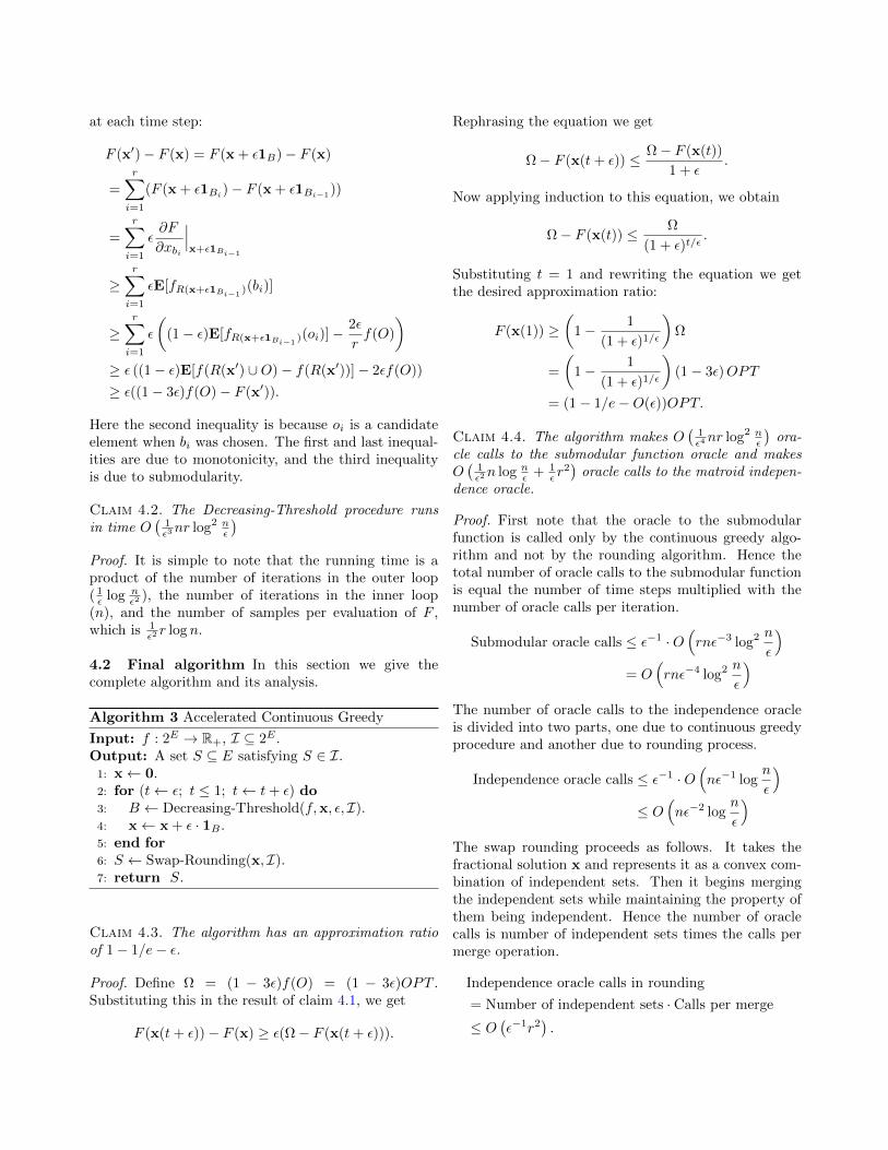
4.2 Final algorithm In this section we give thecomplete algorithm and its analysis.

Algorithm 3 Accelerated Continuous Greedy

Input: f : 2E → R+, I ⊆ 2E .Output: A set S ⊆ E satisfying S ∈ I.1: x← 0.2: for (t← ε; t ≤ 1; t← t+ ε) do3: B ← Decreasing-Threshold(f,x, ε, I).4: x← x + ε · 1B .5: end for6: S ← Swap-Rounding(x, I).7: return S.

Claim 4.3. The algorithm has an approximation ratioof 1− 1/e− ε.

Proof. Define Ω = (1 − 3ε)f(O) = (1 − 3ε)OPT .Substituting this in the result of claim 4.1, we get

F (x(t+ ε))− F (x) ≥ ε(Ω− F (x(t+ ε))).

Rephrasing the equation we get

Ω− F (x(t+ ε)) ≤ Ω− F (x(t))

1 + ε.

Now applying induction to this equation, we obtain

Ω− F (x(t)) ≤ Ω

(1 + ε)t/ε.

Substituting t = 1 and rewriting the equation we getthe desired approximation ratio:

F (x(1)) ≥(

1− 1

(1 + ε)1/ε

)Ω

=

(1− 1

(1 + ε)1/ε

)(1− 3ε)OPT

= (1− 1/e−O(ε))OPT.

Claim 4.4. The algorithm makes O(

1ε4nr log2 n

ε

)ora-

cle calls to the submodular function oracle and makesO(

1ε2n log n

ε + 1ε r

2)

oracle calls to the matroid indepen-dence oracle.

Proof. First note that the oracle to the submodularfunction is called only by the continuous greedy algo-rithm and not by the rounding algorithm. Hence thetotal number of oracle calls to the submodular functionis equal the number of time steps multiplied with thenumber of oracle calls per iteration.

Submodular oracle calls ≤ ε−1 ·O(rnε−3 log2 n

ε

)= O

(rnε−4 log2 n

ε

)The number of oracle calls to the independence oracleis divided into two parts, one due to continuous greedyprocedure and another due to rounding process.

Independence oracle calls ≤ ε−1 ·O(nε−1 log

n

ε

)≤ O

(nε−2 log

n

ε

)The swap rounding proceeds as follows. It takes thefractional solution x and represents it as a convex com-bination of independent sets. Then it begins mergingthe independent sets while maintaining the property ofthem being independent. Hence the number of oraclecalls is number of independent sets times the calls permerge operation.

Independence oracle calls in rounding

= Number of independent sets · Calls per merge

≤ O(ε−1r2

).

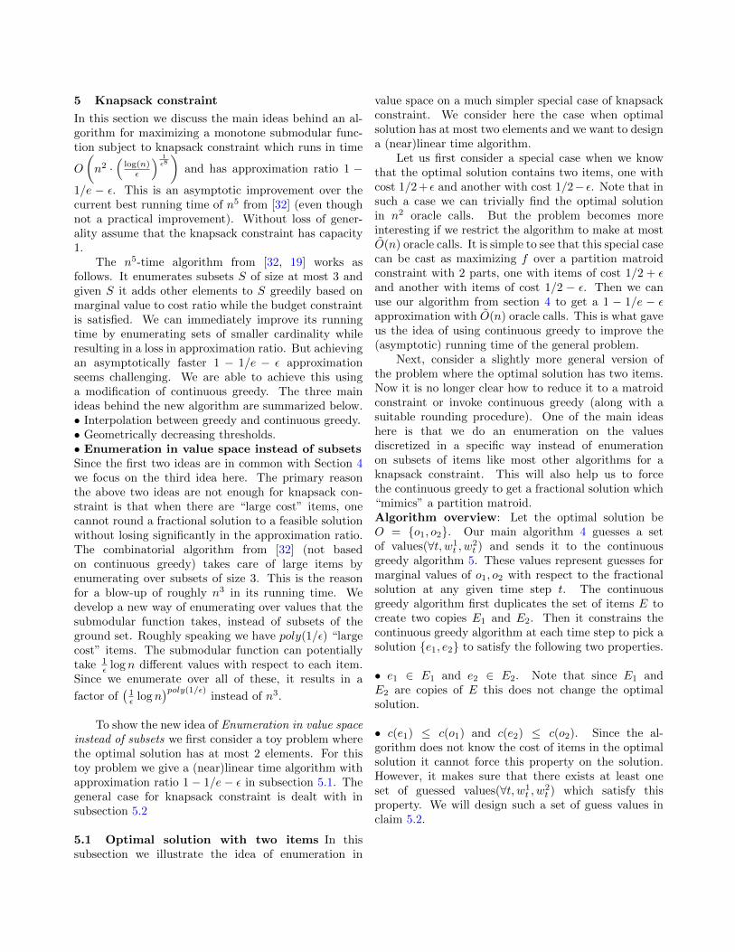
5 Knapsack constraint

In this section we discuss the main ideas behind an al-gorithm for maximizing a monotone submodular func-tion subject to knapsack constraint which runs in time

O

(n2 ·

(log(n)ε

) 1ε8

)and has approximation ratio 1 −

1/e − ε. This is an asymptotic improvement over thecurrent best running time of n5 from [32] (even thoughnot a practical improvement). Without loss of gener-ality assume that the knapsack constraint has capacity1.

The n5-time algorithm from [32, 19] works asfollows. It enumerates subsets S of size at most 3 andgiven S it adds other elements to S greedily based onmarginal value to cost ratio while the budget constraintis satisfied. We can immediately improve its runningtime by enumerating sets of smaller cardinality whileresulting in a loss in approximation ratio. But achievingan asymptotically faster 1 − 1/e − ε approximationseems challenging. We are able to achieve this usinga modification of continuous greedy. The three mainideas behind the new algorithm are summarized below.• Interpolation between greedy and continuous greedy.• Geometrically decreasing thresholds.• Enumeration in value space instead of subsetsSince the first two ideas are in common with Section 4we focus on the third idea here. The primary reasonthe above two ideas are not enough for knapsack con-straint is that when there are “large cost” items, onecannot round a fractional solution to a feasible solutionwithout losing significantly in the approximation ratio.The combinatorial algorithm from [32] (not basedon continuous greedy) takes care of large items byenumerating over subsets of size 3. This is the reasonfor a blow-up of roughly n3 in its running time. Wedevelop a new way of enumerating over values that thesubmodular function takes, instead of subsets of theground set. Roughly speaking we have poly(1/ε) “largecost” items. The submodular function can potentiallytake 1

ε log n different values with respect to each item.Since we enumerate over all of these, it results in a

factor of(1ε log n

)poly(1/ε)instead of n3.

To show the new idea of Enumeration in value spaceinstead of subsets we first consider a toy problem wherethe optimal solution has at most 2 elements. For thistoy problem we give a (near)linear time algorithm withapproximation ratio 1− 1/e− ε in subsection 5.1. Thegeneral case for knapsack constraint is dealt with insubsection 5.2

5.1 Optimal solution with two items In thissubsection we illustrate the idea of enumeration in

value space on a much simpler special case of knapsackconstraint. We consider here the case when optimalsolution has at most two elements and we want to designa (near)linear time algorithm.

Let us first consider a special case when we knowthat the optimal solution contains two items, one withcost 1/2 + ε and another with cost 1/2− ε. Note that insuch a case we can trivially find the optimal solutionin n2 oracle calls. But the problem becomes moreinteresting if we restrict the algorithm to make at mostO(n) oracle calls. It is simple to see that this special casecan be cast as maximizing f over a partition matroidconstraint with 2 parts, one with items of cost 1/2 + εand another with items of cost 1/2 − ε. Then we canuse our algorithm from section 4 to get a 1 − 1/e − εapproximation with O(n) oracle calls. This is what gaveus the idea of using continuous greedy to improve the(asymptotic) running time of the general problem.

Next, consider a slightly more general version ofthe problem where the optimal solution has two items.Now it is no longer clear how to reduce it to a matroidconstraint or invoke continuous greedy (along with asuitable rounding procedure). One of the main ideashere is that we do an enumeration on the valuesdiscretized in a specific way instead of enumerationon subsets of items like most other algorithms for aknapsack constraint. This will also help us to forcethe continuous greedy to get a fractional solution which“mimics” a partition matroid.Algorithm overview: Let the optimal solution beO = o1, o2. Our main algorithm 4 guesses a setof values(∀t, w1

t , w2t ) and sends it to the continuous

greedy algorithm 5. These values represent guesses formarginal values of o1, o2 with respect to the fractionalsolution at any given time step t. The continuousgreedy algorithm first duplicates the set of items E tocreate two copies E1 and E2. Then it constrains thecontinuous greedy algorithm at each time step to pick asolution e1, e2 to satisfy the following two properties.

• e1 ∈ E1 and e2 ∈ E2. Note that since E1 andE2 are copies of E this does not change the optimalsolution.

• c(e1) ≤ c(o1) and c(e2) ≤ c(o2). Since the al-gorithm does not know the cost of items in the optimalsolution it cannot force this property on the solution.However, it makes sure that there exists at least oneset of guessed values(∀t, w1

t , w2t ) which satisfy this

property. We will design such a set of guess values inclaim 5.2.

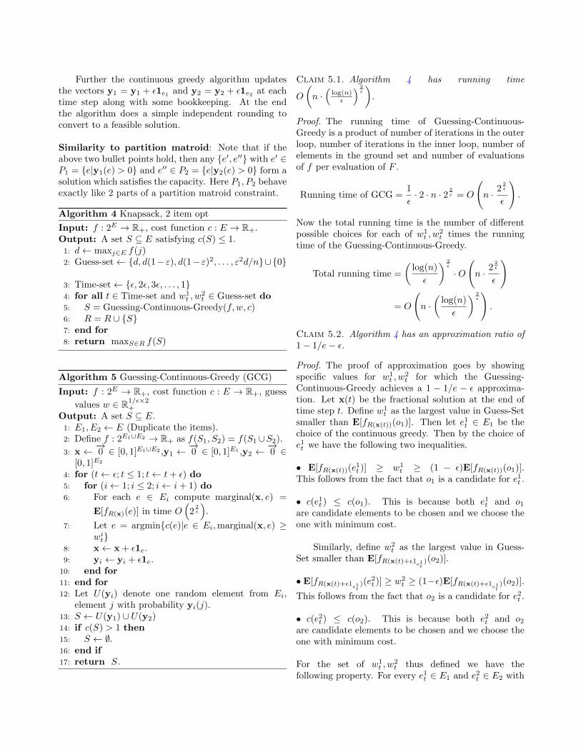
Further the continuous greedy algorithm updatesthe vectors y1 = y1 + ε1e1 and y2 = y2 + ε1e2 at eachtime step along with some bookkeeping. At the endthe algorithm does a simple independent rounding toconvert to a feasible solution.

Similarity to partition matroid: Note that if theabove two bullet points hold, then any e′, e′′ with e′ ∈P1 = e|y1(e) > 0 and e′′ ∈ P2 = e|y2(e) > 0 form asolution which satisfies the capacity. Here P1, P2 behaveexactly like 2 parts of a partition matroid constraint.

Algorithm 4 Knapsack, 2 item opt

Input: f : 2E → R+, cost function c : E → R+.Output: A set S ⊆ E satisfying c(S) ≤ 1.1: d← maxj∈E f(j)2: Guess-set← d, d(1− ε), d(1− ε)2, . . . , ε2d/n∪0

3: Time-set← ε, 2ε, 3ε, . . . , 14: for all t ∈ Time-set and w1

t , w2t ∈ Guess-set do

5: S = Guessing-Continuous-Greedy(f, w, c)6: R = R ∪ S7: end for8: return maxS∈R f(S)

Algorithm 5 Guessing-Continuous-Greedy (GCG)

Input: f : 2E → R+, cost function c : E → R+, guess

values w ∈ R1/ε×2+

Output: A set S ⊆ E.1: E1, E2 ← E (Duplicate the items).2: Define f : 2E1∪E2 → R+ as f(S1, S2) = f(S1∪S2).

3: x ← −→0 ∈ [0, 1]E1∪E2 ,y1 ←−→0 ∈ [0, 1]E1 ,y2 ←

−→0 ∈

[0, 1]E2

4: for (t← ε; t ≤ 1; t← t+ ε) do5: for (i← 1; i ≤ 2; i← i+ 1) do6: For each e ∈ Ei compute marginal(x, e) =

E[fR(x)(e)] in time O(

22ε

).

7: Let e = argminc(e)|e ∈ Ei,marginal(x, e) ≥wit

8: x← x + ε1e.9: yi ← yi + ε1e.

10: end for11: end for12: Let U(yi) denote one random element from Ei,

element j with probability yi(j).13: S ← U(y1) ∪ U(y2)14: if c(S) > 1 then15: S ← ∅.16: end if17: return S.

Claim 5.1. Algorithm 4 has running time

O

(n ·(

log(n)ε

) 2ε

).

Proof. The running time of Guessing-Continuous-Greedy is a product of number of iterations in the outerloop, number of iterations in the inner loop, number ofelements in the ground set and number of evaluationsof f per evaluation of F .

Running time of GCG =1

ε· 2 · n · 2 2

ε = O

(n · 2

2ε

ε

).

Now the total running time is the number of differentpossible choices for each of w1

t , w2t times the running

time of the Guessing-Continuous-Greedy.

Total running time =

(log(n)

ε

) 2ε

·O

(n · 2

2ε

ε

)

= O

(n ·(

log(n)

ε

) 2ε

).

Claim 5.2. Algorithm 4 has an approximation ratio of1− 1/e− ε.

Proof. The proof of approximation goes by showingspecific values for w1

t , w2t for which the Guessing-

Continuous-Greedy achieves a 1 − 1/e − ε approxima-tion. Let x(t) be the fractional solution at the end oftime step t. Define w1

t as the largest value in Guess-Setsmaller than E[fR(x(t))(o1)]. Then let e1t ∈ E1 be thechoice of the continuous greedy. Then by the choice ofe1t we have the following two inequalities.

• E[fR(x(t))(e1t )] ≥ w1

t ≥ (1 − ε)E[fR(x(t))(o1)].This follows from the fact that o1 is a candidate for e1t .

• c(e1t ) ≤ c(o1). This is because both e1t and o1are candidate elements to be chosen and we choose theone with minimum cost.

Similarly, define w2t as the largest value in Guess-

Set smaller than E[fR(x(t)+ε1e1t

)(o2)].

• E[fR(x(t)+ε1e1t

)(e2t )] ≥ w2

t ≥ (1−ε)E[fR(x(t)+ε1e1t

)(o2)].

This follows from the fact that o2 is a candidate for e2t .

• c(e2t ) ≤ c(o2). This is because both e2t and o2are candidate elements to be chosen and we choose theone with minimum cost.

For the set of w1t , w

2t thus defined we have the

following property. For every e1t ∈ E1 and e2t ∈ E2 with

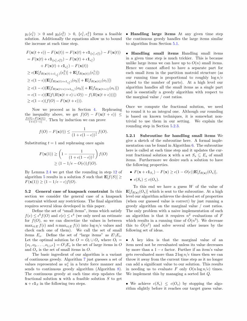
y1(e1t ) > 0 and y2(e2t ) > 0, e1t , e2t forms a feasiblesolution. Additionally the equations allow us to boundthe increase at each time step.

F (x(t+ ε))− F (x(t)) = F (x(t) + ε1e1t ,e2t)− F (x(t))

= F (x(t) + ε1e1t ,e2t)− F (x(t) + ε1e1t )

+ F (x(t) + ε1e1t )− F (x(t))

≥ ε(E[fR(x(t)+ε1e1t

)(e2t )] + E[fR(x(t))(e

1t )])

≥ ε(1− ε)(E[fR(x(t)+ε1e1t

)(o2)] + E[fR(x(t))(o1)])

≥ ε(1− ε)(E[fR(x(t+ε)+ε1o1 )(o2)] + E[fR(x(t+ε))(o1)])

= ε(1− ε)(E[f(R(x(t+ ε) ∪O))− f(R(x(t+ ε)))])

≥ ε(1− ε)(f(O)− F (x(t+ ε))).

Now we proceed as in Section 4. Rephrasingthe inequality above, we get f(O) − F (x(t + ε)) ≤f(O)−F (x(t))

1+ε(1−ε) . Then by induction we can prove

f(O)− F (x(t)) ≤ 1

(1 + ε(1− ε)) tεf(O).

Substituting t = 1 and rephrasing once again

F (x(1)) ≥(

1− 1

(1 + ε(1− ε)) 1ε

)f(O)

≥ (1− 1/e−O(ε))f(O).

By Lemma 2.4 we get that the rounding in step 12 ofalgorithm 5 results in a solution S such that E[f(S)] ≥F (x(1)) ≥ (1− 1/e− ε)f(O).

5.2 General case of knapsack constraint In thissection we consider the general case of a knapsackconstraint without any restrictions. The final algorithmrequires several ideas developed in this paper.

Define the set of “small items”, items which satisfyf(e) ≤ ε6f(O) and c(e) ≤ ε4 (we only need an estimatefor f(O), so we can discretize the values in betweenmaxi∈E f(i) and nmaxi∈E f(i) into log n/ε values andcheck each one of them). We call the set of smallitems Es. Define the set of “large items” as E\Es.Let the optimal solution be O = Ol ∪ Os where Ol =o1, o2, . . . , o1/ε6 = O\Es is the set of large items in Oand Os is the set of small items in O.

The basic ingredient of our algorithm is a variantof continuous greedy. Algorithm 7 just guesses a set ofvalues represented as wit in a brute force manner andsends to continuous greedy algorithm (Algorithm 8).The continuous greedy at each time step updates thefractional solution x with a feasible solution S to getx + ε1S in the following two steps.

• Handling large items At any given time stepthe continuous greedy handles the large items similarto algorithm from Section 5.1.

• Handling small items Handling small itemsin a given time step is much trickier. This is becauseunlike large items we can have up to O(n) small items.Hence we cannot afford to have a separate part foreach small item in the partition matroid structure (asour running time is proportional to roughly log n/εraised to the number of parts). At a high level ouralgorithm handles all the small items as a single partand is essentially a greedy algorithm with respect tothe marginal value / cost ratios.

Once we compute the fractional solution, we needto round it to an integral one. Although our roundingis based on known techniques, it is somewhat non-trivial to use them in our setting. We explain therounding step in Section 5.2.3.

5.2.1 Subroutine for handling small items Wegive a sketch of the subroutine here. A formal imple-mentation can be found in Algorithm 6. The subroutinehere is called at each time step and it updates the cur-rent fractional solution x with a set Ss ⊆ Es of smallitems. Furthermore we desire such a solution to havethe following properties.

• F (x + ε1Ss)− F (x) ≥ ε(1−O(ε))E[fR(x)(Os)],

• c(Ss) ≤ c(Os).

To this end we have a guess W of the value ofE[fR(x)(Os)] which is sent to the subroutine. At a highlevel our algorithm achieves the desired set of properties(when our guessed value is correct) by just running agreedy algorithm on the marginal value / cost ratios.The only problem with a naive implementation of suchan algorithm is that it requires n2 evaluations of Fwhich results in a running time of O(n3). We decreasethis to O(n2) and solve several other issues by thefollowing set of ideas.

• A key idea is that the marginal value of anitem need not be reevaluated unless its value decreasesby more than a 1− ε factor. Further if an item’s valuegets reevaluated more than 2 log n/ε times then we canthrow it away from the current time step as it no longercan add a significant value to our solution. This resultsin needing us to evaluate F only O(n log n/ε) times.We implement this by managing a sorted list Q.

• We achieve c(Ss) ≤ c(Os) by stopping the algo-rithm slightly before it reaches our target guess value.

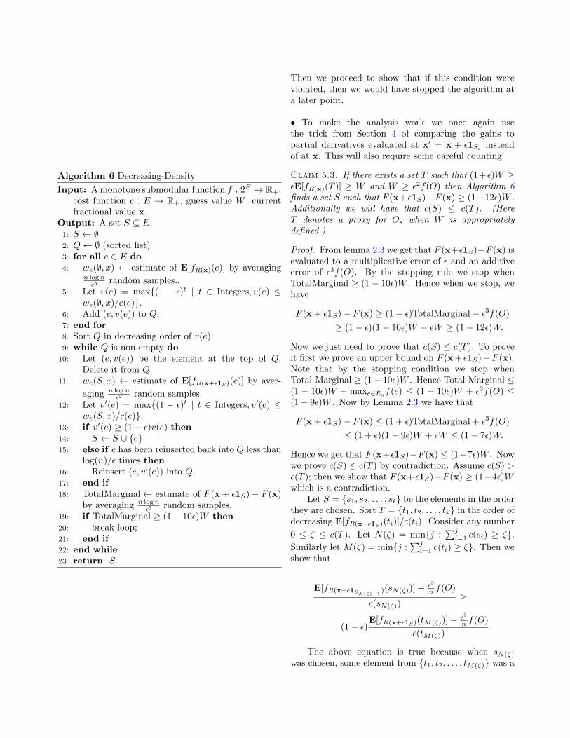
Algorithm 6 Decreasing-Density

Input: A monotone submodular function f : 2E → R+,cost function c : E → R+, guess value W , currentfractional value x.

Output: A set S ⊆ E.1: S ← ∅2: Q← ∅ (sorted list)3: for all e ∈ E do4: we(∅, x) ← estimate of E[fR(x)(e)] by averaging

n lognε3 random samples..

5: Let v(e) = max(1 − ε)t | t ∈ Integers, v(e) ≤we(∅, x)/c(e).

6: Add (e, v(e)) to Q.7: end for8: Sort Q in decreasing order of v(e).9: while Q is non-empty do

10: Let (e, v(e)) be the element at the top of Q.Delete it from Q.

11: we(S, x) ← estimate of E[fR(x+ε1S)(e)] by aver-

aging n lognε2 random samples.

12: Let v′(e) = max(1 − ε)t | t ∈ Integers, v′(e) ≤we(S, x)/c(e).

13: if v′(e) ≥ (1− ε)v(e) then14: S ← S ∪ e15: else if e has been reinserted back into Q less than

log(n)/ε times then16: Reinsert (e, v′(e)) into Q.17: end if18: TotalMarginal← estimate of F (x + ε1S)− F (x)

by averaging n lognε3 random samples.

19: if TotalMarginal ≥ (1− 10ε)W then20: break loop;21: end if22: end while23: return S.

Then we proceed to show that if this condition wereviolated, then we would have stopped the algorithm ata later point.

• To make the analysis work we once again usethe trick from Section 4 of comparing the gains topartial derivatives evaluated at x′ = x + ε1Ss insteadof at x. This will also require some careful counting.

Claim 5.3. If there exists a set T such that (1+ε)W ≥εE[fR(x)(T )] ≥ W and W ≥ ε2f(O) then Algorithm 6finds a set S such that F (x+ε1S)−F (x) ≥ (1−12ε)W .Additionally we will have that c(S) ≤ c(T ). (HereT denotes a proxy for Os when W is appropriatelydefined.)

Proof. From lemma 2.3 we get that F (x+ε1S)−F (x) isevaluated to a multiplicative error of ε and an additiveerror of ε3f(O). By the stopping rule we stop whenTotalMarginal ≥ (1− 10ε)W . Hence when we stop, wehave

F (x + ε1S)− F (x) ≥ (1− ε)TotalMarginal− ε3f(O)

≥ (1− ε)(1− 10ε)W − εW ≥ (1− 12ε)W.

Now we just need to prove that c(S) ≤ c(T ). To proveit first we prove an upper bound on F (x+ ε1S)−F (x).Note that by the stopping condition we stop whenTotal-Marginal ≥ (1− 10ε)W . Hence Total-Marginal ≤(1 − 10ε)W + maxe∈Esf(e) ≤ (1 − 10ε)W + ε3f(O) ≤(1− 9ε)W . Now by Lemma 2.3 we have that

F (x + ε1S)− F (x) ≤ (1 + ε)TotalMarginal + ε3f(O)

≤ (1 + ε)(1− 9ε)W + εW ≤ (1− 7ε)W.

Hence we get that F (x+ε1S)−F (x) ≤ (1−7ε)W . Nowwe prove c(S) ≤ c(T ) by contradiction. Assume c(S) >c(T ); then we show that F (x+ε1S)−F (x) ≥ (1−4ε)Wwhich is a contradiction.

Let S = s1, s2, . . . , s` be the elements in the orderthey are chosen. Sort T = t1, t2, . . . , tk in the order ofdecreasing E[fR(x+ε1S)(ti)]/c(ti). Consider any number

0 ≤ ζ ≤ c(T ). Let N(ζ) = minj :∑ji=1 c(si) ≥ ζ.

Similarly let M(ζ) = minj :∑ji=1 c(ti) ≥ ζ. Then we

show that

E[fR(x+ε1SN(ζ)−1)(sN(ζ))] + ε3

n f(O)

c(sN(ζ))≥

(1− ε)E[fR(x+ε1S)(tM(ζ))]− ε3

n f(O)

c(tM(ζ)).

The above equation is true because when sN(ζ)

was chosen, some element from t1, t2, . . . , tM(ζ) was a

candidate which could have been chosen instead. Nowwe can bound the total gain from S.

F (x + ε1S)− F (x)

=∑i=1

(F (x + ε1Si)− F (x + ε1Si−1))

≥ε∑i=1

E[fR(x+ε1Si−1)(si)]

=ε

∫ c(S)

0

E[fR(x+ε1SN(ζ)−1)(sN(ζ))]

c(sN(ζ))dζ

≥ε∫ c(T )

0

E[fR(x+ε1SN(ζ)−1)(sN(ζ))]

c(sN(ζ))dζ

≥(ε− ε2)

∫ c(T )

0

(E[fR(x+ε1S)(tM(ζ))]− ε3

n f(O)

c(tM(ζ))

−ε3

n f(O)

c(sN(ζ))

)dζ

=∑ti∈T

(ε− ε2)E[fR(x+ε1S)(ti)]− 2ε3f(O)

≥ε(1− ε) (E[f(R(x + ε1S) ∪ T )− f(R(x + ε1S))])

− 2ε3f(O)

≥ε(1− ε) (E[f(R(x) ∪ T )]− F (x + ε1S))− 2ε3f(O)

≥(1− ε) (W − ε(F (x + ε1S)− F (x)))− 2εW.

Rephrasing the equation we get F (x+ε1S)−F (x) ≥(1− 3ε)W/(1 + ε) ≥ (1− 4ε)W which is a contradiction.

Claim 5.4. Algorithm 6 runs in time O(

1ε4n

2 log2 n).

Proof. Note that each item is reinserted back into thesorted list at most log(n)/ε times. Hence the runningtime is at most the product of the total number of items(n), the maximum number of times an item is reinserted(log(n)/ε), and the number of samples per evaluation(n log(n)/ε3).

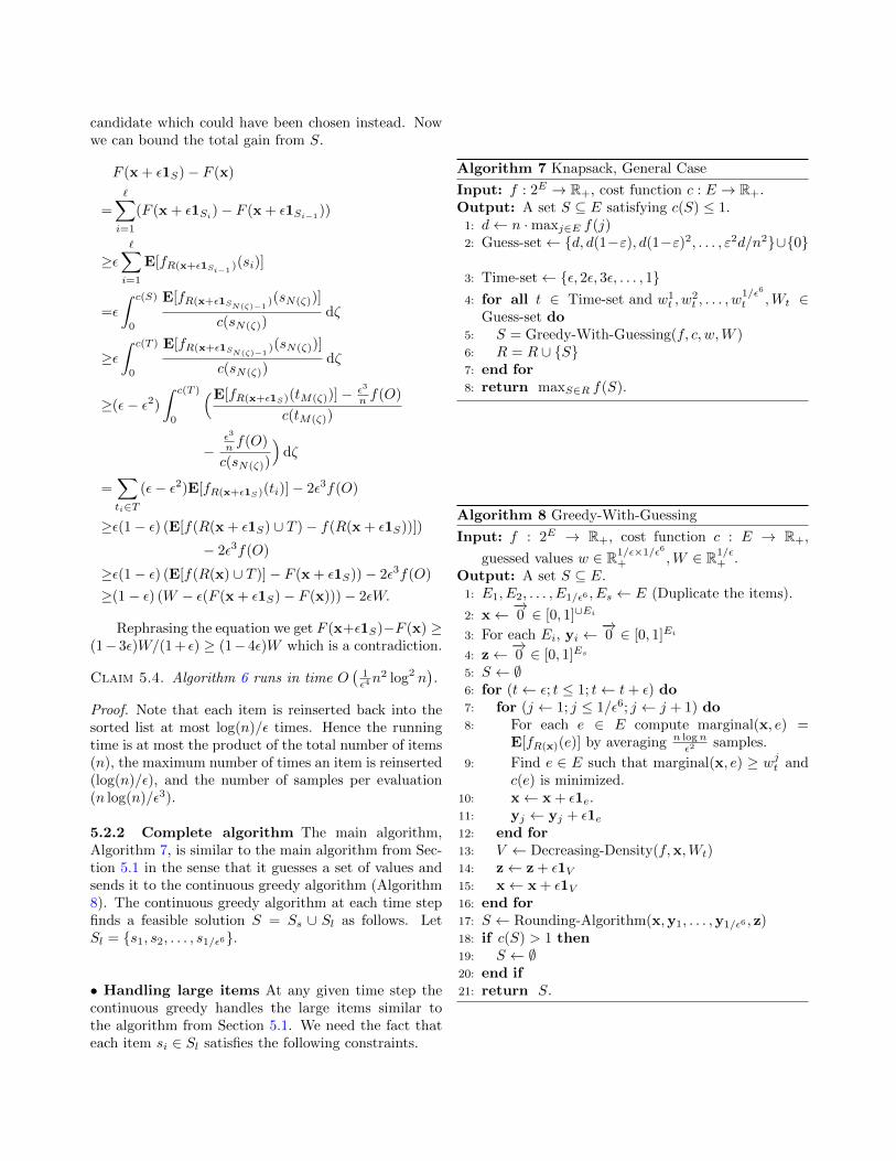
5.2.2 Complete algorithm The main algorithm,Algorithm 7, is similar to the main algorithm from Sec-tion 5.1 in the sense that it guesses a set of values andsends it to the continuous greedy algorithm (Algorithm8). The continuous greedy algorithm at each time stepfinds a feasible solution S = Ss ∪ Sl as follows. LetSl = s1, s2, . . . , s1/ε6.

• Handling large items At any given time step thecontinuous greedy handles the large items similar tothe algorithm from Section 5.1. We need the fact thateach item si ∈ Sl satisfies the following constraints.

Algorithm 7 Knapsack, General Case

Input: f : 2E → R+, cost function c : E → R+.Output: A set S ⊆ E satisfying c(S) ≤ 1.1: d← n ·maxj∈E f(j)2: Guess-set← d, d(1−ε), d(1−ε)2, . . . , ε2d/n2∪0

3: Time-set← ε, 2ε, 3ε, . . . , 14: for all t ∈ Time-set and w1

t , w2t , . . . , w

1/ε6

t ,Wt ∈Guess-set do

5: S = Greedy-With-Guessing(f, c, w,W )6: R = R ∪ S7: end for8: return maxS∈R f(S).

Algorithm 8 Greedy-With-Guessing

Input: f : 2E → R+, cost function c : E → R+,

guessed values w ∈ R1/ε×1/ε6+ ,W ∈ R1/ε

+ .Output: A set S ⊆ E.1: E1, E2, . . . , E1/ε6 , Es ← E (Duplicate the items).

2: x← −→0 ∈ [0, 1]∪Ei

3: For each Ei, yi ←−→0 ∈ [0, 1]Ei

4: z← −→0 ∈ [0, 1]Es

5: S ← ∅6: for (t← ε; t ≤ 1; t← t+ ε) do7: for (j ← 1; j ≤ 1/ε6; j ← j + 1) do8: For each e ∈ E compute marginal(x, e) =

E[fR(x)(e)] by averaging n lognε2 samples.

9: Find e ∈ E such that marginal(x, e) ≥ wjt andc(e) is minimized.

10: x← x + ε1e.11: yj ← yj + ε1e12: end for13: V ← Decreasing-Density(f,x,Wt)14: z← z + ε1V15: x← x + ε1V16: end for17: S ← Rounding-Algorithm(x,y1, . . . ,y1/ε6 , z)18: if c(S) > 1 then19: S ← ∅20: end if21: return S.

- c(si) ≤ c(oi),- E[fR(x+ε1Si−1

)(si)] ≥ (1−O(ε))E[fR(x+ε1Si−1)(oi)].

In Claim 5.6 we design a set of guess values (w) forwhich the above two properties are satisfied.

• Handling small items The subroutine to handlesmall items is described in Section 5.2.1. We need theset returned by the subroutine to satisfy the followingconstraints.- c(Ss) ≤ c(Os),- F (x + ε1S) − F (x + ε1Sl) ≥ (1 −O(ε))E[fR(x+ε1Sl

)(Os)].

Once again we design a set of guess values (W ) inClaim 5.6 for which the above properties are satisfied.

Then the algorithm at the end of each time stepdoes certain bookkeeping on the vectors x,yi andz. Finally it invokes a rounding algorithm which wedescribe in Section 5.2.3.

Claim 5.5. Algorithm 7 has running time

O

(n2 ·

(log(n)ε

) 1ε8

).

Proof. It is straightforward to see that the runningtime of each instantiation of continuous greedy isO(n2 log2 n/ε9). The total running time is a productof this with number of possible choices for w.

Running time ≤(

log(n)

ε

)1/ε7

· n2 log2 n

ε9

=O

(n2 ·

(log(n)

ε

)1/ε8).

Claim 5.6. Algorithm 7 has approximation ratio 1 −1/e−O(ε).

Proof. The proof is by designing a sequence of w forwhich the algorithm Greedy-With-Guessing gives a 1−1/e− ε approximation.

For each step define wit as the maximum number inthe guess-set smaller than E[fR(x(t)+ε1Si−1

)(oi)]. Then

by the choice of ei we have the following two properties.• E[fR(x(t),Si−1)(ei)] + ε

nf(O) ≥ wit ≥ (1 −ε)E[fR(x(t),Si−1)(oi)]. This follows from the factthat oi is a candidate for ei.• c(ei) ≤ c(oi).

Define Wt as the largest value in Guess-Set smallerthan εE[fR(x(t)+ε1Sl )

(Os)]. Then from Claim 5.3 of thesection for handling small items we have that• F (x(t) + ε1Sl∪Ss) − F (x(t) + ε1Sl) ≥ ε(1 −12ε)E[fR(x(t)+ε1Sl )

(Os)].

• c(Ss) ≤ c(Os).

For the set of wit,Wt thus defined we will see thata simple rounding in Section 5.2.3 returns a feasiblesolution. Additionally we can bound the increase ateach time step as follows.

F (x(t+ ε))− F (x(t))

=

1/ε6∑i=1

(F (x(t) + ε1Si−1∪ei)− F (x(t) + ε1Si−1

))

+F (x(t) + ε1Sl∪Ss)− F (x(t) + ε1Sl)

≥ ε

1/ε6∑i=1

E[fR(x(t)+ε1Si−1)(ei)]

+F (x(t) + ε1Sl∪Ss)− F (x(t) + ε1Sl)

≥ ε(1− ε)

1/ε6∑i=1

E[fR(x(t)+ε1Si−1)(oi)]−

ε

nf(O)

+ε(1− 12ε)E[fR(x(t)+ε1Sl )

(Os)]− ε2f(O)

= ε(1− ε)1/ε6∑i=1

(E[f(R(x(t) + ε1Si−1) ∪ oi)

−f(R(x(t) + ε1Si−1))])− ε2f(O)

+ε(1− 12ε)E[f(R(x(t) + ε1Sl) ∪Os)−f(R(x(t) + ε1Sl))]− ε2f(O)

≥ ε(1− ε)1/ε6∑i=1

(E[f(R(x(t) + ε1S) ∪Oi)

−f(R(x(t) + ε1S) ∪Oi−1)])

+ε(1− 12ε)E[f(R(x(t) + ε1S) ∪Os)−f(R(x(t) + ε1S))]− 2ε2f(O)

= ε(1− ε)(E[f(R(x(t) + ε1S) ∪Ol)−f(R(x(t) + ε1S))])

+ε(1− 12ε)E[f(R(x(t) + ε1S) ∪Os)−f(R(x(t) + ε1S))]− 2ε2f(O)

≥ ε(1− ε)(E[f(R(x(t) + ε1S) ∪O)

−f(R(x(t) + ε1S) ∪Os)])+ε(1− 12ε)E[f(R(x(t) + ε1S) ∪Os)

−f(R(x(t) + ε1S))]− 2ε2f(O)

≥ ε(1− 12ε)E[f(R(x(t) + ε1S) ∪O)

−f(R(x(t) + ε1S))]− 2ε2f(O)

≥ ε(1− 14ε)(f(O)− F (x(t+ ε))).

Now we proceed similarly to the analysis of continu-ous greedy for a matroid constraint. Rephrasing we get

f(O) − F (x(t + ε)) ≤ f(O)−F (x(t))1+ε(1−14ε) . Then by induction

we can prove

f(O)− F (x(t)) ≤(

1

(1 + ε(1− 14ε))tε

)f(O).

Now substituting t = 1 and rephrasing once again

F (x(1)) ≥(

1− 1

(1 + ε(1− 14ε))1ε

)f(O)

≥ (1− 1/e−O(ε))f(O).

5.2.3 Rounding In this subsection we show how toconvert a fractional solution as produced by Algorithm 7to an integral solution. We restrict our attention to thefractional solution x,y1,y2, . . . ,y1/ε6 , z correspond-ing to the values w,W designed in Lemma 5.6 for whichwe have the following properties.

• F (x) ≥ (1− 1/e−O(ε))f(O).

• x =∑1/εi=1 ε1Sεi where Sεi is the set chosen at time

εi.

• The set chosen at time t, St = Sl,t ∪ Ss,t canbe represented as a union of large items (Sl,t =s1,t, s2,t, . . . , s1/ε6,t) and small items (Ss,t). LetO = Ol ∪Os with Ol = o1, o2, . . . , o1/ε6

• For each time t and each si,t ∈ Sl,t we have thatsi,t ∈ Ei. Additionally Ss,t ⊆ Es.

• For each time t and each si,t ∈ Sl,t we have thatc(si,t) ≤ c(oi).

• For each time t we have that c(Ss,t) ≤ c(Os).

Now from the above properties one can see that for anygiven i since c(si,t) ≤ c(oi) we can choose any of theelements ∪tsi,t and it will be a good substitute foroi. Now applying Lemma 2.4 we shall not lose anythingin the approximation ratio. The rounding is formallydescribed in Algorithm 9.

Algorithm 9 Rounding-Algorithm

Input: Fractional solution x = z+∑ 1

ε6

i=1 yi =∑t ε1St .

Output: A set S ⊆ E satisfying c(S) ≤ 1 andE[f(S)] ≥ (1− ε)F (x)

1: Sl, Ss ← ∅2: Define z′ ∈ [0, 1]Es as z′(e) = z(e) if c(e) <ε3 maxi c(Ss,t) and z′(e) = 0 otherwise.

3: for i = 1, 2, . . . , 1/ε6 do4: Include one of e ∈ Ei to Sl with e being included

with probability yi(e).5: end for6: For each e ∈ Es, include in Ss independently with

probability (1− ε)z′(e).7: S ← Sl ∪ Ss.8: return S.

Claim 5.7. Algorithm 9 rounds the fractional solutionto a set S such that E[f(S)] ≥ (1− ε)F (x).

Proof. First let us relate value of the fractional solutionx = z +

∑t yt to that of x′ = z′ +

∑t y.

F (x′) =F

(z′ +

∑t

yt

)

≥F

(z +

∑t

yt

)−

∑c(e)≥ε3 maxi c(Ss,t)

z(e)f(e)

≥F (x)−maxe∈Es

f(e)∑

c(e)≥ε3 maxi c(Ss,t)

z(e)

≥F (x)−(ε6f(O)

) 1

ε3

≥F (x)− ε3f(O)

≥(1− ε)F (x).

Next we note that we get S by selecting exactly one ran-dom element from each Ei, and sampling independentlyfrom Es. Hence applying Lemma 2.4 we get

E[f(S)] ≥ F ((1−ε)x′) ≥ (1−ε)F (x′) ≥ (1−O(ε))F (x).

Claim 5.8. Algorithm 9 rounds the fractional solutionto a set S such that with high probability c(S) ≤ 1. i.eS is a feasible solution to the knapsack constraint.

Proof. Note that by the condition that for each i,c(si,t) ≤ c(oi) the large items after the rounding willhave cost less than the large items of the optimalsolution. Hence it is enough to prove that with highprobability c(Ss) ≤ c(Os). First note that

E[c(R((1− ε)z′))] = (1− ε)E[c(R(z′))]

≤ (1− ε)E[c(R(z))]

≤ (1− ε) maxtc(Ss,t) ≤ (1− ε)c(Os).

Additionally we have that for each element e withz′(e) > 0 we have that c(e) ≤ ε3c(Os). Hence we boundthe probability that c(Ss) > c(Os) by a simple Chernoffbound (Lemma 2.2) to show this happens with very lowprobability. We set up the Chernoff bound with Xe =c(e)/(ε3c(Os)) if e ∈ Ss and Xe = 0 otherwise. ThenE[X] =

∑eE[Xe] = E[c(R((1 − ε)z′))]/(ε3c(Os)) ≤

(1− ε)/ε3. Therefore, we obtain

Pr[c(Ss) > c(Os)] = Pr[X ≥ ε−3]

≤ e−ε2

31ε3 ≤ e− 1

3ε ≤ 3ε.

6 p-system and ` knapsack constraints

Here we consider a more general type of constraint: ap-system combined with ` knapsack constraints. (We

refer the reader to Section 2 for the definition of a p-system.) This is the most general type of constraint thatwe handle in this paper. As special cases, this containsthe intersection of p matroids and ` knapsacks, as wellas p-set packing combined with ` knapsack constraints.We assume without loss of generality that each knapsackconstraint has unit capacity.

Algorithm 10 p-system and ` knapsack constraints

Input: f : 2E → R+, a membership oracle for p-system I ⊂ 2E , and ` knapsack-cost functionsci : E → [0, 1].

Output: A set S ⊆ E satisfying S ∈ I and ci(S) ≤ 1∀i.

1: M ← maxj∈E f(j)2: repeat the following for ρ ∈ Mp+` , (1 + ε) M

p+` , (1 +

ε)2 Mp+` , . . . ,

2nMp+` (density threshold)

3: τ ← Mρ ← maxf(j) : f(j)∑`i=1 cij

≥ ρ (value

threshold)4: S ← ∅5: while τ ≥ ε

nMρ and ci(S) ≤ 1∀i do6: for ∀j ∈ E do

7: if S + j ∈ I and fS(j) ≥ τ and fS(j)∑`i=1 cij

≥ ρ

then8: S ← S + j9: if ∃i; ci(S) > 1 then

10: Sρ ← S, Tρ ← S \ j, T ′ρ ← j11: restart with the next value of ρ12: end if13: end if14: end for15: τ ← 1

1+ετ16: end while17: Tρ ← Sρ ← S, T ′ρ ← ∅18: restart with the next value of ρ19: return the set of maximum value among Tρ and

T ′ρ for all enumerations of ρ.

Algorithm overview: We define the density of an

element j with respect to a set S as fS(j)∑`i=1 cij

. Our

algorithm combines two ideas:

• a fixed density threshold ρ, which is somewhatbelow the value/size ratio of the optimal solution; thisis guessed (i.e. enumerated) by the algorithm,

• a decreasing value threshold τ , which mimicsthe greedy algorithm for p-systems but leads to a fasterrunning time.

In each stage, the algorithm picks all items that

are above the density threshold and also above thevalue threshold. The value threshold decreases slightlyafter each stage. This is effectively a greedy algorithmwith respect to marginal values, while discarding allelements of density below some threshold. The greedyrule guarantees an approximation ratio for a p-systemconstraint, while the density threshold guarantees thatwe do not exceed the knapsack constraints withoutcollecting enough value.

For a formal description, see Algorithm 10. We callthe execution of the algorithm for a given value of ρ a“run of the algorithm”. We call the inner loop for agiven value of τ a “stage of the algorithm”.

Theorem 6.1. Algorithm 10 runs in time O( nε2 log2 nε )

and provides a (1 + ε)(p+ 2`+ 1)-approximation for theproblem of maximizing a monotone submodular functionsubject to a p-system and ` knapsack constraints.

We note that we consider p, ` to be constant; i.e.,the O notation hides a constant depending on p, `.This constant is actually very mild - linear in `, andindependent of p (this is due to our model whichassumes a membership oracle for the p-system). Thefollowing claim gives a more accurate statement ofrunning time.

Claim 6.1. The running time of Algorithm 10 isO(` nε2 log2 n

ε ).

Proof. The enumeration loop consists of log1+ε(2n)values of ρ. The decreasing-threshold loop consists oflog1+ε

nε values of τ . The inner loop checks each element

of E, querying its marginal value and performing anO(`) time computation. Therefore, the total runningtime is

O(`n log1+ε(2n) log1+ε

n

ε

)= O

(`n

ε2log2 n

ε

).

For the analysis of the approximation ratio, let usintroduce some notation: We fix an optimal solution O.Given a density threshold ρ and the resulting solutionSρ, we denote

O<ρ = j ∈ O :fSρ(j)∑`i=1 cij

< ρ

and O≥ρ = O \O<ρ.

Claim 6.2. Given ρ and the respective algorithmic so-lution Sρ, we have

fSρ(O<ρ) ≤ `ρ.

Proof. By the definition of O<ρ, for each j ∈ O<ρwe have fSρ(j) < ρ

∑`i=1 cij . By submodularity,

fSρ(O<ρ) ≤∑j∈O<ρ fSρ(j) ≤ ρ

∑`i=1

∑j∈O<ρ cij ≤ ρ`

by the feasibility of O and O<ρ being a subset of O.

Claim 6.3. If the algorithm terminates without exceed-ing any knapsack constraint, we have

fSρ(O≥ρ) ≤ ((1 + ε)p+ ε) · f(Sρ).

The proof of this claim is essentially the analysisof the greedy algorithm for a p-system, as in [2]. Wesupply the proof for completeness.

Proof. Consider the elements of Sρ in the order they areadded by the algorithm: denote them by e1, e2, . . . , er.For i ∈ 1, . . . , r, we define a set Ai ⊆ O≥ρ \ Sρ,consisting of the elements that could have been addedinstead of ei:

Ai = j ∈ O≥ρ \ Sρ : e1, . . . , ei−1, j ∈ I.

We also define Ar+1 in the same way; these are theelements in O≥ρ \ Sρ that could still be added to Sρat the end of the run. Since O≥ρ \ Sρ ∈ I, we haveA1 = O≥ρ \ Sρ. By the down-monotonicity of I, itfollows that O≥ρ \ Sρ = A1 ⊇ A2 ⊇ A3 ⊇ . . . Ar+1.

Next, we use the defining property of p-systems.Consider the set Qi = e1, . . . , ei ∪ (A1 \ Ai+1). Wehave A1 \ Ai+1 ∈ I, hence Qi has a base of size atleast |A1 \ Ai+1|. On the other hand, e1, . . . , ei isalso a base of Qi, since no element of A1 \ Ai+1 can beadded to e1, . . . , ei (otherwise by definition it wouldbe in Ai+1). Since I is a p-system, the cardinality ofthe two bases cannot differ by a factor larger than p;equivalently, |A1 \Ai+1| ≤ pi.

Now consider the stages of the algorithm definedby decreasing τ . For 1 ≤ i ≤ r, define τi to be thevalue of the threshold τ when ei was included in Sρ.In particular, the marginal value of ei at that pointis fe1,...,ei−1(ei) ≥ τi. For each j ∈ Ai, if j wereconsidered at a stage earlier than ei, j would have beenadded to Sρ because its density would have been aboveρ (by submodularity) and adding it to e1, . . . , ei−1would not violate feasibility in I. (Also, we assumedthat no knapsack constraint overflows in this run ofthe algorithm). However, j /∈ Sρ, and hence j couldnot have been considered before ei. This implies thatfe1,...,ei−1(j) ≤ (1 + ε)τi, for each j ∈ Ai.

By a similar argument, for each j ∈ Ar+1, wehave fSρ(j) <

εnMρ (the lowest possible value of the

threshold τ ; see the algorithm for definition of Mρ),otherwise j would still be added to Sρ = e1, . . . , er.In fact, it can be seen that the first element chosen by

the algorithm is of value exactly Mρ, and τ1 = Mρ.Therefore, fSρ(j) ≤ ε

nτ1 for all j ∈ Ar+1.It remains to add up the values of all the elements

in A1 = O≥ρ \ Sρ, marginally with respect to Sρ. Bysubmodularity, we have

fSρ(A1) ≤∑j∈A1

fSρ(j)

=

r∑i=1

∑j∈Ai\Ai+1

fSρ(j) +∑

j∈Ar+1

fSρ(j).

As we proved, fSρ(j) ≤ fe1,...,ei−1(j) ≤ (1 + ε)τi forj ∈ Ai \ Ai+1, and fSρ(j) ≤ ε

nτ1 for j ∈ Ar+1. So weobtain

fSρ(A1) ≤ (1 + ε)

r∑i=1

|Ai \Ai+1|τi + |Ar+1|ε

nτ1.

We proved above that |A1 \ Ai+1| ≤ pi. Also, observethat due to the operation of the algorithm, τ1 ≥ τ2 ≥τ3 ≥ . . .. Under these conditions, the right-hand sideis maximized when |Ai \ Ai+1| = p for each 1 ≤ i ≤ r.Thus we obtain

fSρ(A1) ≤ (1 + ε)

r∑i=1

pτi + |Ar+1|ε

nτ1

≤ (1 + ε)

r∑i=1

pτi + ετ1.

Recall that τi was the value of the threshold τ when eiwas included; this implies that fe1,...,ei−1(ei) ≥ τi, i.e.f(Sρ) ≥

∑ri=1 τi. Therefore,

fSρ(O≥ρ) = fSρ(A1) ≤ (1 + ε)p · f(Sρ) + ε · f(Sρ).

Let us proceed to the proof of Theorem 6.1.

Proof. Consider an optimal solution O and set ρ∗ =2

p+2`+1f(O). Since M ≤ f(O) ≤ nM (by submod-

ularity), we have ρ∗ ∈ [ Mp+` ,2nMp+` ]. Thus there is a

run of the algorithm with density threshold ρ such thatρ∗ ∈ [ρ, (1 + ε)ρ]. In the following we consider this runof the algorithm. We consider two cases.

(1) If the algorithm terminates by exceeding someknapsack capacity, then we obtain a set Sρ such that

ci(Sρ) > 1 for some i ∈ [`]. I.e., certainly∑`i=1 ci(Sρ) >

1. Since every element that we include satisfies fS(j) ≥ρ∑`i=1 cij , with respect to the current solution S, we

obtain

f(Sρ) ≥ ρ∑i=1

∑j∈Sρ

cij > ρ.

This solution is infeasible; however, we keep eitherTρ = Sρ \ j or T ′ρ = j where j is the last element

included in Sρ. Each of these solutions is feasible andby submodularity, one of them has value at least 1

2ρ. Byour choice of ρ ≥ 1

1+ερ∗ = 2

(1+ε)(p+2`+1)f(O), we obtain

maxf(Tρ), f(T ′ρ) ≥1

2ρ ≥ 1

(1 + ε)(p+ 2`+ 1)f(O).

(2) If the algorithm terminates without exceedingany knapsack capacity, then by the above claims,

fSρ(O<ρ) ≤ `ρ ≤ `ρ∗ =2`

p+ 2`+ 1f(O)

and

fSρ(O≥ρ) ≤ ((1 + ε)p+ ε) · f(Sρ).

By submodularity,

fSρ(O) ≤ fSρ(O<ρ) + fSρ(O≥ρ)

≤ 2`

p+ 2`+ 1f(O) + ((1 + ε)p+ ε) · f(Sρ).

Since fSρ(O) = f(Sρ ∪O)− f(Sρ) ≥ f(O)− f(Sρ), thismeans

f(O) ≤ 2`

p+ 2`+ 1f(O) + (1 + ε)(p+ 1) · f(Sρ)

and from here

(1 + ε)f(Sρ) ≥1

p+ 2`+ 1f(O).

Again, f(Sρ) ≥ 1(1+ε)(p+2`+1)f(O), which proves the

theorem.

7 A lower bound for p-systems

Theorem 7.1. For any ε > 0, a 1/(p + ε)-approximation for the problem max|S| : S ∈ I,where I is a p-system, requires an exponential numberof queries to I.

Proof. The proof is by constructing two p-systemsP1, P2 ⊂ 2E randomly, with p · max|S| : S ∈ P1 =max|S| : S ∈ P2, such that it requires an exponen-tial number of queries to distinguish between them withconstant probability. We define the two set systems asfollows.

• Define t = n/(4p) (where n = |E|) and let S ⊆ Ebe in P1 iff |S| ≤ t.

• Let T be a set of size pt chosen uniformly at randomfrom

(Ept

). Then let S be in P2 iff either |S| ≤ t or

S ⊆ T .

It is easy to verify that P1 and P2 are both p-systems: for P1 it is trivial, and for P2 all maximal baseshave size between t and pt. Also, max|S| : S ∈ P1 = tand max|S| : S ∈ P2 = pt.

Now consider any query S. S can distinguishbetween P1 and P2 iff t < |S| ≤ pt and S ⊆ T . Fixany S with t < |S| ≤ pt. Then S ⊆ T with probability( pt|S|)( n|S|)

over the random choice of T. Furthermore, as long

as S 6⊆ T , we do not learn anything about whether theset system is P2 or the identity of T . Hence we needto make Ω(

(n|S|)/(pt|S|)) queries to distinguish P1 from P2

with constant probability. From here,

# Queries required = Ω

((n|S|)(

pt|S|)) ≥ Ω

((n− |S|)|S|

(pt)|S|

)

≥ Ω

((n− ptpt

)t)= Ω

(3n/(4p)

).

References

[1] Niv Buchbinder, Moran Feldman, Joseph Naor, andRoy Schwartz. A tight linear time (1/2)-approximationfor unconstrained submodular maximization. InFOCS, 2012. 2

[2] Gruia Calinescu, Chandra Chekuri, Martin Pal, andJan Vondrak. Maximizing a monotone submodularfunction subject to a matroid constraint. SIAM J.Comput., 40(6):1740–1766, 2011. 2, 3, 4, 5, 16

[3] Chandra Chekuri, Jan Vondrak, and Rico Zenklusen.Submodular function maximization via the multilin-ear relaxation and contention resolution schemes. InSTOC, pages 783–792, 2011. 2, 3, 5, 6

[4] Shahar Dobzinski and Michael Schapira. An improvedapproximation algorithm for combinatorial auctionswith submodular bidders. In SODA, pages 1064–1073,2006. 1

[5] Devdatt P. Dubhashi and Alessandro Panconesi. Con-centration of Measure for the Analysis of RandomizedAlgorithms. Cambridge University Press, 2009. 4

[6] Uriel Feige. On maximizing welfare when utilityfunctions are subadditive. In STOC, pages 41–50,2006. 1

[7] Uriel Feige, Vahab S. Mirrokni, and Jan Vondrak.Maximizing non-monotone submodular functions. InFOCS, pages 461–471, 2007. 2

[8] Uriel Feige and Jan Vondrak. Approximation algo-rithms for allocation problems: Improving the factorof 1 - 1/e. In FOCS, pages 667–676, 2006. 1

[9] Moran Feldman, Joseph Naor, and Roy Schwartz.Nonmonotone submodular maximization via a struc-tural continuous greedy algorithm - (extended ab-stract). In ICALP, pages 342–353, 2011. 2

[10] Moran Feldman, Joseph Naor, and Roy Schwartz. Aunified continuous greedy algorithm for submodularmaximization. In FOCS, pages 570–579, 2011. 2

[11] Yuval Filmus and Justin Ward. A tight combinatorialalgorithm for submodular maximization subject to amatroid constraint. CoRR, abs/1204.4526, 2012. 2, 3

[12] M. L. Fisher, G. L. Nemhauser, and L. A. Wolsey. Ananalysis of approximations for maximizing submodularset functions - II. Math. Prog. Study, 8:73–87, 1978. 1,2, 3

[13] Shayan Oveis Gharan and Jan Vondrak. Submodularmaximization by simulated annealing. In SODA, pages1098–1116, 2011. 2

[14] Carlos Guestrin, Andreas Krause, and Ajit Paul Singh.Near-optimal sensor placements in gaussian processes.In ICML, pages 265–272, 2005. 1

[15] Anupam Gupta, Viswanath Nagarajan, and R. Ravi.Robust and maxmin optimization under matroid andknapsack uncertainty sets. CoRR, abs/1012.4962,2010. 2

[16] Anupam Gupta, Aaron Roth, Grant Schoenebeck, andKunal Talwar. Constrained non-monotone submodularmaximization: Offline and secretary algorithms. InWINE, pages 246–257, 2010. 2

[17] David Kempe, Jon M. Kleinberg, and Eva Tardos.Maximizing the spread of influence through a socialnetwork. In KDD, pages 137–146, 2003. 1

[18] David Kempe, Jon M. Kleinberg, and Eva Tardos. In-fluential nodes in a diffusion model for social networks.In ICALP, pages 1127–1138, 2005. 1

[19] Samir Khuller, Anna Moss, and Joseph Naor. Thebudgeted maximum coverage problem. Inf. Process.Lett., 70(1):39–45, 1999. 8

[20] Andreas Krause and Carlos Guestrin. Submodularityand its applications in optimized information gather-ing. ACM TIST, 2(4):32, 2011. 1

[21] Andreas Krause, Carlos Guestrin, Anupam Gupta, andJon M. Kleinberg. Near-optimal sensor placements:maximizing information while minimizing communica-tion cost. In IPSN, pages 2–10, 2006. 1

[22] Andreas Krause, Carlos Guestrin, Anupam Gupta,and Jon M. Kleinberg. Robust sensor placementsat informative and communication-efficient locations.TOSN, 7(4):31, 2011. 1

[23] Andreas Krause, Ajit Paul Singh, and Carlos Guestrin.Near-optimal sensor placements in gaussian processes:Theory, efficient algorithms and empirical studies.Journal of Machine Learning Research, 9:235–284,2008. 1, 2

[24] Ariel Kulik, Hadas Shachnai, and Tami Tamir. Max-imizing submodular set functions subject to multiplelinear constraints. In SODA, pages 545–554, 2009. 2,3

[25] Jon Lee, Vahab S. Mirrokni, Viswanath Nagarajan,and Maxim Sviridenko. Non-monotone submodularmaximization under matroid and knapsack constraints.In STOC, pages 323–332, 2009. 2

[26] Jon Lee, Maxim Sviridenko, and Jan Vondrak. Ma-

troid matching: the power of local search. In STOC,pages 369–378, 2010. 2, 4

[27] Benny Lehmann, Daniel J. Lehmann, and Noam Nisan.Combinatorial auctions with decreasing marginal util-ities. Games and Economic Behavior, 55(2):270–296,2006. 1

[28] Jure Leskovec, Andreas Krause, Carlos Guestrin,Christos Faloutsos, Jeanne M. VanBriesen, and Na-talie S. Glance. Cost-effective outbreak detection innetworks. In KDD, pages 420–429, 2007. 1, 2

[29] G. L. Nemhauser and L. A. Wolsey. Best algorithmsfor approximating the maximum of a submodular setfunctions. Math. Oper. Research, 3(3):177–188, 1978.1

[30] G. L. Nemhauser, L. A. Wolsey, and M. L. Fisher. Ananalysis of approximations for maximizing submodularset functions - I. Math. Prog., 14:265–294, 1978. 1, 3

[31] Alexander Schrijver. Combinatorial Optimization,Volume B. Springer, 2003. 4

[32] Maxim Sviridenko. A note on maximizing a submodu-lar set function subject to a knapsack constraint. Oper.Res. Lett., 32(1):41–43, 2004. 2, 3, 8

[33] Jan Vondrak. Optimal approximation for the submod-ular welfare problem in the value oracle model. InSTOC, pages 67–74, 2008. 1, 2, 3, 5

[34] Jan Vondrak. Symmetry and approximability of sub-modular maximization problems. In FOCS, pages 651–670, 2009. 2