Maximizing non-monotone submodular functions∗

Uriel Feige †

Dept. of Computer Science and Applied MathematicsThe Weizmann Institute

Rehovot, Israeluriel.feige@weizmann.ac.il

Vahab S. Mirrokni ‡

Google ResearchNew York, NY

mirrokni@google.com

Jan Vondrak §

IBM Alamaden Research CenterSan Jose, CA

jvondrak@us.ibm.com

January 29, 2011

Abstract

Submodular maximization generalizes many important problems including Max Cut in directedand undirected graphs and hypergraphs, certain constraint satisfaction problems and maximum fa-cility location problems. Unlike the problem of minimizing submodular functions, the problem ofmaximizing submodular functions is NP-hard.

In this paper, we design the first constant-factor approximation algorithms for maximizing non-negative (non-monotone) submodular functions. In particular, we give a deterministic local-search13-approximation and a randomized 2

5-approximation algorithm for maximizing nonnegative submod-

ular functions. We also show that a uniformly random set gives a 14-approximation. For symmetric

submodular functions, we show that a random set gives a 12-approximation, which can be also achieved

by deterministic local search.These algorithms work in the value oracle model where the submodular function is accessible

through a black box returning f(S) for a given set S. We show that in this model, a ( 12

+ ε)-approximation for symmetric submodular functions would require an exponential number of queriesfor any fixed ε > 0. In the model where f is given explicitly (as a sum of nonnegative submodularfunctions, each depending only on a constant number of elements), we prove NP-hardness of ( 5

6+ ε)-

approximation in the symmetric case and NP-hardness of ( 34

+ ε)-approximation in the general case.

∗An extended abstract of this paper appeared in FOCS’07 [14].†This work was done while the author was at Microsoft Research, Redmond, WA.‡This work was done while the author was at Microsoft Research, Redmond, WA.§This work was done while the author was at Microsoft Research and Princeton University.

1 Introduction

We consider the problem of maximizing a nonnegative submodular function. This means, given a sub-modular function f : 2X → R+, we want to find a set S ⊆ X maximizing f(S).

Definition 1.1. A function f : 2X → R is submodular if for any S, T ⊆ X,

f(S ∪ T ) + f(S ∩ T ) ≤ f(S) + f(T ).

An alternative definition of submodularity is the property of decreasing marginal values: For anyA ⊆ B ⊆ X and x ∈ X \B, f(B ∪ {x})− f(B) ≤ f(A∪ {x})− f(A). This can be deduced from the firstdefinition by substituting S = A ∪ {x} and T = B; the reverse implication also holds.

We assume value oracle access to the submodular function; i.e., for a given set S, an algorithm canquery an oracle to find its value f(S).

Background. Submodularity, a discrete analog of convexity, has played an essential role in combina-torial optimization [35]. It appears in many important settings including cuts in graphs [21, 42, 18], rankfunction of matroids [10, 19], set covering problems [12], and plant location problems [8, 9]. In manysettings such as set covering or matroid optimization, the relevant submodular functions are monotone,meaning that f(S) ≤ f(T ) whenever S ⊆ T . Here, we are more interested in the general case where f(S)is not necessarily monotone. A canonical example of such a submodular function is f(S) =

∑e∈δ(S) w(e),

where δ(S) is a cut in a graph (or hypergraph) induced by a set of vertices S and w(e) is the weightof edge e. Cuts in undirected graphs and hypergraphs yield symmetric submodular functions, satisfyingf(S) = f(S) for all sets S. Symmetric submodular functions have been considered widely in the litera-ture [17, 42]. It appears that symmetry allows better/simpler approximation results, and thus deservesseparate attention.

The problem of maximizing a submodular function is of central importance, with special cases includ-ing Max Cut [21], Max Directed Cut [26], hypergraph cut problems, maximum facility location [1, 8, 9],and certain restricted satisfiability problems [27, 11]. While the Min Cut problem in graphs is a classicalpolynomial-time solvable problem, and more generally it has been shown that any submodular functioncan be minimized in polynomial time [45, 18], maximization turns out to be more difficult and indeed allthe aforementioned special cases are NP-hard.

A related problem is Max-k-Cover, where the goal is to choose k sets whose union is as large aspossible. It is known that a greedy algorithm provides a (1 − 1/e)-approximation for Max-k-Cover andthis is optimal unless P = NP [12]. More generally, this problem can be viewed as maximization of amonotone submodular function under a cardinality constraint, i.e. max{f(S) : |S| ≤ k}, assuming fsubmodular and 0 ≤ f(S) ≤ f(T ) whenever S ⊆ T . Again, the greedy algorithm provides a (1 − 1/e)-approximation for this problem [39] and this is optimal in the oracle model [40]. More generally, a(1 − 1/e)-approximation can be achieved for monotone submodular maximization under a knapsackconstraint [46]. For the problem of maximizing a monotone submodular function subject to a matroidconstraint, the greedy algorithm gives only a 1

2 -approximation [16]. Recently, this has been improved toan optimal (1− 1/e)-approximation using the multilinear extension of a submodular function [49, 6].

In contrast, here we consider the unconstrained maximization of a submodular function which isnot necessarily monotone. We only assume that the function is nonnegative.1 Typical examples ofsuch a problem are Max Cut and Max Directed Cut. Here, the best approximation factors have beenachieved using semidefinite programming: 0.878 for Max Cut [21] and 0.874 for Max Di-Cut [11, 31]. Theapproximation factor for Max Cut has been proved optimal, assuming the Unique Games Conjecture [29,38]. Without the use of semidefinite programming, only 1

2 -approximation for Max Cut was known for along time. For Max Di-Cut, a combinatorial 1

2 -approximation was presented in [26]. Recently, Trevisangave a 0.53-approximation algorithm for Max Cut using a spectral partitioning method [48].

1For submodular functions without any restrictions, verifying whether the maximum of the function is greater than zerois NP-hard and requires exponentially many queries in the value oracle model. Thus, no efficient approximation algorithmcan be found for general submodular maximization. For a general submodular function f with minimum value f0, we candesign an approximation algorithm to maximize a normalized submodular function g where g(S) = f(S)− f0.

1

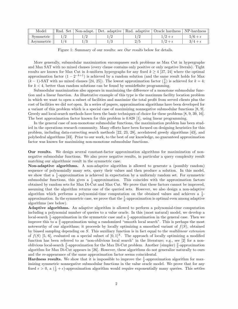
Model Rnd. Set Non-adapt. Det. adaptive Rnd. adaptive Oracle hardness NP-hardness

Symmetric 1/2 1/2 1/2 1/2 1/2 + ε 5/6 + εAsymmetric 1/4 1/3 1/3 2/5 1/2 + ε 3/4 + ε

Figure 1: Summary of our results: see Our results below for details.

More generally, submodular maximization encompasses such problems as Max Cut in hypergraphsand Max SAT with no mixed clauses (every clause contains only positive or only negative literals). Tightresults are known for Max Cut in k-uniform hypergraphs for any fixed k ≥ 4 [27, 24] where the optimalapproximation factor (1 − 2−k+1) is achieved by a random solution (and the same result holds for Max(k − 1)-SAT with no mixed clauses [24, 25]). The lowest approximation factor ( 7

8 ) is achieved for k = 4;for k < 4, better than random solutions can be found by semidefinite programming.

Submodular maximization also appears in maximizing the difference of a monotone submodular func-tion and a linear function. An illustrative example of this type is the maximum facility location problemin which we want to open a subset of facilities and maximize the total profit from served clients plus thecost of facilities we did not open. In a series of papers, approximation algorithms have been developed fora variant of this problem which is a special case of maximizing nonnegative submodular functions [8, 9].Greedy and local-search methods have been the basic techniques of choice for these problems [8, 9, 39, 16].The best approximation factor known for this problem is 0.828 [1], using linear programming.

In the general case of non-monotone submodular functions, the maximization problem has been stud-ied in the operations research community. Many efforts have been focused on designing heuristics for thisproblem, including data-correcting search methods [22, 23, 28], accelatered greedy algorithms [43], andpolyhedral algorithms [33]. Prior to our work, to the best of our knowledge, no guaranteed approximationfactor was known for maximizing non-monotone submodular functions.

Our results. We design several constant-factor approximation algorithms for maximization of non-negative submodular functions. We also prove negative results, in particular a query complexity resultmatching our algorithmic result in the symmetric case.Non-adaptive algorithms. A non-adaptive algorithm is allowed to generate a (possibly random)sequence of polynomially many sets, query their values and then produce a solution. In this model,we show that a 1

4 -approximation is achieved in expectation by a uniformly random set. For symmetricsubmodular functions, this gives a 1

2 -approximation. This coincides with the approximation factorsobtained by random sets for Max Di-Cut and Max Cut. We prove that these factors cannot be improved,assuming that the algorithm returns one of the queried sets. However, we also design a non-adaptivealgorithm which performs a polynomial-time computation on the obtained values and achieves a 1

3 -approximation. In the symmetric case, we prove that the 1

2 -approximation is optimal even among adaptivealgorithms (see below).Adaptive algorithms. An adaptive algorithm is allowed to perform a polynomial-time computationincluding a polynomial number of queries to a value oracle. In this (most natural) model, we develop alocal-search 1

2 -approximation in the symmetric case and a 13 -approximation in the general case. Then we

improve this to a 25 -approximation using a randomized “smooth local search”. This is perhaps the most

noteworthy of our algorithms; it proceeds by locally optimizing a smoothed variant of f(S), obtainedby biased sampling depending on S. This auxiliary function is in fact equal to the multilinear extensionof f(S) [5, 6], evaluated on a special subset of [0, 1]X . The approach of locally optimizing a modifiedfunction has been referred to as “non-oblivious local search” in the literature; e.g., see [2] for a non-oblivious local-search 2

5 -approximation for the Max Di-Cut problem. Another (simpler) 25 -approximation

algorithm for Max Di-Cut appears in [26]. However, these algorithms do not generalize naturally to oursand the re-appearance of the same approximation factor seems coincidental.Hardness results. We show that it is impossible to improve the 1

2 -approximation algorithm for max-imizing symmetric nonnegative submodular functions in the value oracle model. We prove that for anyfixed ε > 0, a ( 1

2 + ε)-approximation algorithm would require exponentially many queries. This settles

2

the status of symmetric submodular maximization in the value oracle model. Note that this query com-plexity lower bound does not assume any computational restrictions. In contrast, in the special case ofMax Cut, polynomially many value queries suffice to infer all edge weights in the graph, and thereafteran exponential time computation (involving no further queries) would actually produce the optimal cut.

For explicitly represented submodular functions, known inapproximability results for Max Cut ingraphs and hypergraphs provide an obvious limitation to the best possible approximation ratio. Weprove stronger limitations. For any fixed ε > 0, it is NP-hard to achieve an approximation factor of34 + ε (or 5

6 + ε) in the general (or symmetric) case, respectively. These results are valid even when thesubmodular function is given as a sum of polynomially many nonnegative submodular functions, eachdepending only on a constant number of elements, which is the case for the aforementioned special casessuch as Max Cut.

Follow-up research. Following the conference version of this paper, several developments have beenmade in the area of submodular maximization, some of them inspired by the results and techniques inthis paper. In particular, local-search constant-factor approximation algorithms have been developed formaximizing a non-monotone submodular function subject to multiple knapsack (linear) constraints ormultiple matroid constraints [32], and these algorithms have been further improved in [34, 50]. For max-imizing monotone submodular functions, optimal approximation algorithms have been developed in thecases of a matroid constraint [49, 6], and multiple knapsack constraints [30]. For the problem consideredin this paper, maximization of a non-monotone submodular function, an improved 0.41-approximationhas been found [41], and hardness of 0.695-approximation has been proved for explicit instances, assumingthe unique games conjecture [4].

The idea behind the information-theoretic lower bounds in this paper has been generalized to provehardness results for other problems, including social welfare maximization in combinatorial auctionswith submodular bidders [36], and non-monotone submodular maximization subject to matroid baseconstraints [50]. A more general connection has been made between the approximability of submodu-lar maximization problems and properties of their multilinear relaxation [50], which can be seen as ageneralization of the hardness construction in this paper (Section 4.2).

It has been also shown that submodular functions can be approximated point-wise within an O(√n)

factor using a polynomial number of value queries. This is optimal up to logarithmic factors [20]. Relatedto this phenomenon are several O(

√n)-approximation algorithms for submodular minimization under

various constraints [47, 20].

Preliminaries. We use the following form of the Chernoff bound (see [3, Theorem A.1.16]).

Theorem 1.2. Let Y1, . . . , Yt be independent random variables in [−1, 1] such that E[Yi] = 0. Then

Pr[

t∑i=1

Yi > λ] ≤ e−λ2/2t.

2 Non-adaptive algorithms

It is known that simply choosing a random cut is a good choice for Max Cut and Max Di-Cut, achievingan approximation factor of 1/2 and 1/4 respectively. We show the natural role of submodularity here bypresenting the same approximation factors in the general case of submodular functions.

The Random Set Algorithm: RS.Let X(p) denote a random subset of X, where each element is sampled independently with probability p.

• Return R = X(1/2).

Theorem 2.1. Let f : 2X → R+ be a submodular function, OPT = maxS⊆X f(S) and let R denote auniformly random subset R = X(1/2). Then E[f(R)] ≥ 1

4OPT. In addition, if f is symmetric (f(S) =f(X \ S) for every S ⊆ X), then E[f(R)] ≥ 1

2OPT.

3

Before proving this result, we show a useful probabilistic property of submodular functions (extendingthe considerations of [13, 15]). This property will be essential in the analysis of our improved randomizedalgorithm as well.

Lemma 2.2. Let g : 2X → R be submodular. Denote by A(p) a random subset of A where each elementappears with probability p. Then

E[g(A(p))] ≥ (1− p) g(∅) + p g(A).

Proof. By induction on the size of A: For A = ∅, the lemma is trivial. So assume A = A′ ∪ {x}, x /∈ A′.Then A(p)∩A′ is a subset of A′ where each element appears with probability p; hence we denote it A′(p).By submodularity, g(A(p))− g(A′(p)) ≥ g(A(p) ∪A′)− g(A′), and therefore

E[g(A(p))] ≥ E[g(A′(p)) + g(A(p) ∪A′)− g(A′)]

= E[g(A′(p))] + E[g(A(p) ∪A′)− g(A′)]

= E[g(A′(p))] + p (g(A)− g(A′)).

Applying the inductive hypothesis, E[g(A′(p))] ≥ (1 − p) g(∅) + p g(A′), we get the statement of thelemma.

By a double application of Lemma 2.2, we obtain the following.

Lemma 2.3. Let f : 2X → R be submodular, A,B ⊆ X two (not necessarily disjoint) sets and A(p), B(q)their independently sampled subsets, where each element of A appears in A(p) with probability p and eachelement of B appears in B(q) with probability q. Then

E[f(A(p) ∪B(q))] ≥ (1− p)(1− q) f(∅) + p(1− q) f(A) + (1− p)q f(B) + pq f(A ∪B).

Proof. Condition on A(p) = R and define g(T ) = f(R ∪ T ). This is a submodular function as well andLemma 2.2 implies E[g(B(q))] ≥ (1−q) f(R)+q f(R∪B). Also, E[g(B(q))] = E[f(A(p)∪B(q)) | A(p) =R], and by unconditioning: E[f(A(p) ∪ B(q))] ≥ E[(1 − q) f(A(p)) + q f(A(p) ∪ B)]. Finally, we applyLemma 2.2 once again: E[f(A(p))] ≥ (1−p) f(∅) +p f(A), and by applying the same to the submodularfunction h(S) = f(S ∪B), E[f(A(p) ∪B)] ≥ (1− p) f(B) + p f(A ∪B). This implies the claim.

This lemma gives immediately the performance of Algorithm RS.

Proof. Denote the optimal set by S and its complement by S. We can write R = S(1/2)∪ S(1/2). UsingLemma 2.3, we get

E[f(R)] ≥ 1

4f(∅) +

1

4f(S) +

1

4f(S) +

1

4f(X).

Every term is nonnegative and f(S) = OPT , so we get E[f(R)] ≥ 14OPT. In addition, if f is symmetric,

we also have f(S) = OPT and then E[f(R)] ≥ 12OPT.

As we show in Section 4.2, 14 -approximation is optimal for non-adaptive algorithms that are required

to return one of the queried sets. Here, we show that it is possible to design a 13 -approximation algorithm

which queries a polynomial number of sets non-adaptively and then returns a possibly different set after apolynomial-time computation. The intuition behind the algorithm comes from the Max Di-Cut problem:When does a random cut achieve only 1/4 of the optimum? This is if and only if the optimum containsall the directed edges of the graph, i.e. the vertices can be partitioned into V = A ∪ B so that all edgesof the graph are directed from A to B. However, in this case it is easy to find the optimal solution,by a local test on the in-degree and out-degree of each vertex. In the language of submodular functionmaximization, this means that elements can be easily partitioned into those whose inclusion in S alwaysincreases the value of f(S), and those which always decrease f(S). Our generalization of this local testis the following.

4

Definition 2.4. Let R = X(1/2) denote a uniformly random subset of X. For each element x, define

ω(x) = E[f(R ∪ {x})− f(R \ {x})].

Note that the expectation E[f(R)], for any distribution of R, can be estimated by random samplingup to an additive error polynomially small relative to OPT . More precisely, we use the following lemma.

Lemma 2.5. If f : 2X → R, R1, . . . , Rt are independent samples from some distribution on 2X , andE[f(Ri)] = µ for all i, then ∣∣∣∣∣1t

t∑i=1

f(Ri)− µ

∣∣∣∣∣ ≤ εmax f(S)

with probability at least 1− 2e−tε2/2, for any ε ∈ [0, 1].

Proof. Let M = max f(S); f(R) is a random variable in the range [0,M ]. Let Yi = 1M (f(Ri) − µ)

where Ri is the i-th random sample. We have Yi ∈ [−1, 1], these random variables are independent, andE[Yi] = 0. By Theorem 1.2,

Pr

[∣∣∣1t

t∑i=1

f(Ri)− µ∣∣∣ > εM

]= Pr

[∣∣∣ t∑i=1

Yi

∣∣∣ > tε

]≤ 2e−tε

2/2.

This is sufficient for our purposes; we use ε = 1/poly(n), t = n/ε2, and obtain with high probabilityestimates with additive error OPT/poly(n). In the following, we assume that we have estimates forquantities like E[f(R)] and ω(x) within additive error OPT/poly(n).

The Non-Adaptive Algorithm: NA.

• Use random sampling to find ω(x) for each x ∈ X, such that |ω(x)− ω(x)| < 1n2OPT w.h.p.

• Independently, sample a random set R = X(1/2).

• With prob. 8/9, return R.

• With prob. 1/9, return A = {x ∈ X : ω(x) > 0}.

Theorem 2.6. For any nonnegative submodular function, Algorithm NA achieves expected value at least(1/3− o(1)) OPT .

Proof. Let A = {x ∈ X : ω(x) > 0} and B = X \ A = {x ∈ X : ω(x) ≤ 0}. Therefore we haveω(x) ≥ −OPT/n2 for any x ∈ A and ω(x) ≤ OPT/n2 for any x ∈ B. We shall keep in mind that (A,B)is a partition of all the elements, and so we have (A ∩ T ) ∪ (B ∩ T ) = T for any set T , etc.

Denote by C the optimal set, f(C) = OPT . Let f(A) = α, f(B ∩ C) = β and f(B ∪ C) = γ. Bysubmodularity, we have

α+ β = f(A) + f(B ∩ C) ≥ f(∅) + f(A ∪ (B ∩ C)) ≥ f(A ∪ C)

andα+ β + γ ≥ f(A ∪ C) + f(B ∪ C) ≥ f(X) + f(C) ≥ OPT.

Therefore, either α, the value of A, is at least OPT/3, or else one of β and γ is at least OPT/3; we provethat then E[f(R)] ≥ OPT/3 as well.

Let us start with β = f(B∩C). Instead of E[f(R)], we show that it is enough to estimate E[f(R∪(B∩C))]. Recall that for any x ∈ B, we have ω(x) = E[f(R∪{x})−f(R\{x})] ≤ OPT/n2. Consequently, we

5

also have E[f(R∪{x})−f(R)] = 12ω(x) ≤ OPT/(2n2). Let us order the elements of B∩C = {b1, . . . , b`}

and write

f(R ∪ (B ∩ C)) = f(R) +∑j=1

(f(R ∪ {b1, . . . , bj})− f(R ∪ {b1, . . . , bj−1})).

By the property of decreasing marginal values, we get

f(R ∪ (B ∩ C)) ≤ f(R) +∑j=1

(f(R ∪ {bj})− f(R)) = f(R) +∑

x∈B∩C(f(R ∪ {x})− f(R))

and therefore

E[f(R ∪ (B ∩ C))] ≤ E[f(R)] +∑

x∈B∩CE[f(R ∪ {x})− f(R)]

≤ E[f(R)] + |B ∩ C|OPT2n2

≤ E[f(R)] +OPT

2n.

So it is enough to lower-bound E[f(R ∪ (B ∩ C))]. We do this by defining a new submodular function,g(R) = f(R∪(B∩C)), and applying Lemma 2.3 to E[g(R)] = E[g(C(1/2)∪C(1/2))]. The lemma impliesthat

E[f(R ∪ (B ∩ C))] ≥ 1

4g(∅) +

1

4g(C) +

1

4g(C) +

1

4g(X)

≥ 1

4g(∅) +

1

4g(C) =

1

4f(B ∩ C) +

1

4f(C) =

β

4+OPT

4.

Note that β ≥ OPT/3 implies E[f(R∪(B∩C))] ≥ OPT/3. Symmetrically, we show a similar analysis forE[f(R∩(B∪C))]. Now we use the fact that for any x ∈ A, E[f(R)−f(R\{x})] = 1

2ω(x) ≥ −OPT/(2n2).Let A \ C = {a1, a2, . . . , ak} and write

f(R) = f(R \ (A \ C)) +

k∑j=1

(f(R \ {aj+1, . . . , ak})− f(R \ {aj , . . . , ak}))

≥ f(R \ (A \ C)) +

k∑j=1

(f(R)− f(R \ {aj})

using the condition of decreasing marginal values. Note that R \ (A \ C) = R ∩ (B ∪ C). By taking theexpectation,

E[f(R)] ≥ E[f(R ∩ (B ∪ C))] +

k∑j=1

E[f(R)− f(R \ {aj})]

= E[f(R ∩ (B ∪ C))]− |A \ C|OPT2n2

≥ E[f(R ∩ (B ∪ C))]− OPT

2n.

Again, we estimate E[f(R ∩ (B ∪ C))] = E[f(C(1/2) ∪ (B \ C)(1/2))] using Lemma 2.3. We get

E[f(R ∩ (B ∪ C))] ≥ 1

4f(∅) +

1

4f(C) +

1

4f(B \ C) +

1

4f(B ∪ C) ≥ OPT

4+γ

4.

Now we combine our estimates for E[f(R)]:

E[f(R)] +OPT

2n≥ 1

2E[f(R ∪ (B ∩ C))] +

1

2E[f(R ∩ (B ∪ C))] ≥ OPT

4+β

8+γ

8.

Finally, the expected value obtained by the algorithm is

8

9E[f(R)] +

1

9f(A) ≥ 2

9OPT − 4

9nOPT +

β

9+γ

9+α

9≥(

1

3− 4

9n

)OPT

since α+ β + γ ≥ OPT .

6

3 Adaptive algorithms

We turn to adaptive algorithms for the problem of maximizing a general nonnegative submodular function.We propose several algorithms improving the 1

4 -approximation achieved by a random set.

3.1 Deterministic local search

Here, we present a deterministic 13 -approximation algorithm. Our deterministic algorithm is based on a

simple local-search technique. We try to increase the value of our solution S by either including a newelement in S or discarding one of the elements of S. We call S a local optimum if no such operationincreases the value of S. Local optima have the following property which was first observed in [7, 23].

Lemma 3.1. Given a submodular function f , if S is a local optimum of f , and T ⊆ S or T ⊇ S, thenf(T ) ≤ f(S).

This property turns out to be very useful in comparing a local optimum to the global optimum.However, it is known that finding a local optimum for the Max Cut problem is PLS-complete [44].Therefore, we relax our local search and find an approximate local optimal solution.

Local Search Algorithm: LS.

1. Let S := {v} where f({v}) is the maximum over all singletons v ∈ X.

2. If there exists an element a ∈ X\S such that f(S ∪ {a}) > (1 + εn2 )f(S), then let S := S ∪ {a},

and go back to Step 2.

3. If there exists an element a ∈ S such that f(S\{a}) > (1 + εn2 )f(S), then let S := S\{a}, and go

back to Step 2.

4. Return the maximum of f(S) and f(X\S).

It is easy to see that if the algorithm terminates, the set S is a (1 + εn2 )-approximate local optimum,

in the following sense.

Definition 3.2. Given f : 2X → R, a set S is called a (1+α)-approximate local optimum, if (1+α)f(S) ≥f(S \ {v}) for any v ∈ S, and (1 + α)f(S) ≥ f(S ∪ {v}) for any v /∈ S.

We prove the following analogue of Lemma 3.1.

Lemma 3.3. If S is an (1 +α)-approximate local optimum for a submodular function f then for any setT such that T ⊆ S or T ⊇ S, we have f(T ) ≤ (1 + nα)f(S).

Proof. Let T = T1 ⊆ T2 ⊆ . . . ⊆ Tk = S be a chain of sets where Ti\Ti−1 = {ai}. For each 2 ≤ i ≤ k,we know that f(Ti)− f(Ti−1) ≥ f(S)− f(S \ {ai}) ≥ −αf(S) using the submodularity and approximatelocal optimality of S. Summing up these inequalities, we get f(S) − f(T ) ≥ −kαf(S). Thus f(T ) ≤(1 + kα)f(S) ≤ (1 + nα)f(S). This completes the proof for set T ⊆ S. The proof for T ⊇ S is verysimilar.

Theorem 3.4. Algorithm LS is a(

13 −

εn

)-approximation algorithm for maximizing nonnegative submod-

ular functions, and a(

12 −

εn

)-approximation algorithm for maximizing nonnegative symmetric submod-

ular functions. The algorithm uses at most O( 1εn

3 log n) oracle calls.

Proof. Consider an optimal solution C and let α = εn2 . If the algorithm terminates, the set S obtained

at the end is a (1 + α)-approximate local optimum. By Lemma 3.3, (1 + nα)f(S) ≥ f(S ∩ C) and(1 + nα)f(S) ≥ f(S ∪ C). Using submodularity, f(S ∪ C) + f(X\S) ≥ f(C\S) + f(X) ≥ f(C\S), andf(S ∩ C) + f(C\S) ≥ f(C) + f(∅) ≥ f(C). Putting these inequalities together, we get

2(1 + nα)f(S) + f(X\S) ≥ f(S ∩ C) + f(S ∪ C) + f(X\S)

≥ f(S ∩ C) + f(C\S) ≥ f(C).

7

For α = εn2 , this implies that either f(S) ≥ ( 1

3 −εn )OPT or f(X\S) ≥ ( 1

3 −εn )OPT .

For symmetric submodular functions, we use Lemma 3.3 to obtain the inequality (1 + nα)f(S) ≥f(S ∪ C), and therefore

2(1 + nα)f(S) ≥ f(S ∩ C) + f(S ∪ C) = f(S ∩ C) + f(S ∩ C) ≥ f(C)

and hence f(S) is a ( 12 −

εn )-approximation.

To bound the running time of the algorithm, let v be a singleton of maximum value f({v}). It issimple to see that OPT ≤ nf({v}). After each iteration, the value of the function increases by a factor ofat least (1 + ε

n2 ). Therefore, if we iterate k times, then f(S) ≥ (1 + εn2 )kf({v}) and yet f(S) ≤ nf({v}),

hence k = O( 1εn

2 log n). The number of queries is O( 1εn

3 log n).

Tight example. Consider a submodular function defined as a cut function in a directed graph D =(V,A). The graph has 4 vertices, V = {a, b, c, d} and 4 arcs, A = {(a, b), (b, c), (c, b), (c, d)}. The cutfunction f(S) denotes the number of arcs leaving S. The optimum solution is S∗ = {a, c} which givesa cut of size f(S∗) = 3. However, the algorithm LS could terminate with the set S = {a, b} which is alocal optimum of value f(S) = 1 (switching any element keeps the objective value the same).

3.2 Randomized local search

Next, we present a randomized algorithm which improves the approximation ratio of 1/3 to 2/5. Themain idea behind this algorithm is to find a “smoothed” local optimum, where elements are sampledrandomly but with different probabilities, based on some underlying set A. The general approach oflocal search, based on a function derived from the one we are interested in, has been referred to as“non-oblivious local search” in the literature [2]. The auxiliary function we are trying to optimize is themultilinear extension of f(S) (see [5, 6]):

F (x) =∑S⊆X

f(S)∏i∈S

xi∏j /∈S

(1− xj).

Definition 3.5. We say that a set is sampled with bias δ based on A, if elements in A are sampled inde-pendently with probability p = 1+δ

2 and elements outside of A are sampled independently with probability

q = 1−δ2 . We denote this random set by R(A, δ).

Observe that the expected value E[f(R(A, δ))] is equal to F (x) evaluated at a point x ∈ [0, 1]X whosecoordinates have only two distinct values, p and q. The set A describes exactly those coordinates whosevalue is p. Our algorithm effectively performs a local search over such points.

The Smooth Local Search algorithm: SLS.

1. Fix parameters δ, δ′ ∈ [−1, 1]. Start with A = ∅. Let n = |X| denote the total number of elements.In the following, use an estimate for OPT , for example from Algorithm LS.

2. For each element x, define

ωA,δ(x) = E[f(R(A, δ) ∪ {x})]−E[f(R(A, δ) \ {x})].

By repeated sampling, we compute ωA,δ(x), an estimate of ωA,δ(x) within ± 1n2OPT w.h.p.

3. If there is x ∈ X \A such that ωA,δ(x) > 2n2OPT , include x in A and go to Step 2.

4. If there is x ∈ A s.t. ωA,δ(x) < − 2n2OPT , remove x from A and go to Step 2.

5. Return a random set R(A, δ′), for a suitably chosen δ′.

8

In effect, we find an approximate local optimum of a derived function Φ(A) = E[f(R(A, δ))]. Thenwe return a set sampled according to R(A, δ′); possibly for δ′ 6= δ. One can run Algorithm SLS with

δ = δ′ and prove that the best approximation for such parameters is achieved by setting δ = δ′ =√

5−12 ,

the golden ratio. Then, we get an approximation factor of 3−√

52 − o(1) ' 0.38. (We omit the proof here.)

However, our best result is achieved by taking a combination of two choices as follows.

Theorem 3.6. Algorithm SLS runs in polynomial time. If we run SLS with δ = 1/3 and δ′ is chosenrandomly to be 1/3 with probability 0.9, or −1 with probability 0.1, the expected value of the solution isat least ( 2

5 − o(1))OPT .

Proof. Let Φ(A) = E[f(R(A, δ))]. We set B = X\A. Recall that inR(A, δ), elements from A are sampledwith probability p = 1+δ

2 , while elements from B are sampled with probability q = 1−δ2 . Consider Step

3 where an element x is added to A. Let A′ = A ∪ {x} and B′ = B \ {x}. The reason why x is added toA is that ωA,δ(x) > 2

n2OPT ; i.e. ωA,δ(x) > 1n2OPT . During this step, Φ(A) increases by

Φ(A′)− Φ(A) = E[f(A′(p) ∪B′(q))− f(A(p) ∪B(q))]

= (p− q) E[f(A(p) ∪B′(q) ∪ {x})− f(A(p) ∪B′(q))]= δ E[f(R(A, δ) ∪ {x})− f(R(A, δ) \ {x})]

= δ ωA,δ(x) >δ

n2OPT.

Similarly, executing Step 4 increases Φ(A) by at least δn2OPT . Since the value of Φ(A) is always between

0 and OPT , the algorithm cannot iterate more than n2/δ times and thus it runs in polynomial time.From now on, let A be the set at the end of the algorithm and B = X \A. We also use R = A(p)∪B(q)

to denote a random set from the distribution R(A, δ). We denote by C the optimal solution, while ouralgorithm returns either R (for δ′ = δ) or B (for δ′ = −1). When the algorithm terminates, we haveωA,δ(x) ≥ − 3

n2OPT for any x ∈ A, and ωA,δ(x) ≤ 3n2OPT for any x ∈ B. Consequently, for any x ∈ B

we have E[f(R ∪ {x}) − f(R)] = Pr[x /∈ R]E[f(R ∪ {x}) − f(R \ {x})] = 23ωA,δ(x) ≤ 2

n2OPT , usingPr[x /∈ R] = p = 2/3. By submodularity, we get

E[f(R ∪ (B ∩ C))] ≤ E[f(R)] +∑

x∈B∩CE[f(R ∪ {x})− f(R))]

≤ E[f(R)] + |B ∩ C| 2

n2OPT

≤ E[f(R)] +2

nOPT.

Similarly, we can obtain E[f(R ∩ (B ∪ C))] ≤ E[f(R)] + 2nOPT. This means that instead of R, we can

analyze R ∪ (B ∩ C) and R ∩ (B ∪ C). In order to estimate E[f(R ∪ (B ∩ C))] and E[f(R ∩ (B ∪ C))],we use a further extension of Lemma 2.3 which can be proved by another iteration of the same proof:

(∗) E[f(A1(p1) ∪A2(p2) ∪A3(p3))] ≥∑

I⊆{1,2,3}

∏i∈I

pi∏i/∈I

(1− pi) f

(⋃i∈I

Ai

).

First, we deal with R ∩ (B ∪ C) = (A ∩ C)(p) ∪ (B ∩ C)(q) ∪ (B \ C)(q). We plug in δ = 1/3, i.e.p = 2/3 and q = 1/3. Then (*) yields

E[f(R ∩ (B ∪ C))] ≥ 8

27f(A ∩ C) +

2

27f(B ∪ C) +

2

27f(B ∩ C) +

4

27f(C) +

4

27f(F ) +

1

27f(B)

where we denote F = (A∩C)∪ (B \C) and we discarded the terms f(∅) ≥ 0 and f(B \C) ≥ 0. Similarly,we estimate E[f(R∪ (B∩C))], applying (*) to a submodular function h(R) = f(R∪ (B∩C)) and writingE[f(R ∪ (B ∩ C))] = E[h(R)] = E[h((A ∩ C)(p) ∪ (A \ C)(p) ∪B(q))]:

E[f(R ∪ (B ∩ C))] ≥ 8

27f(A ∪ C) +

2

27f(B ∪ C) +

2

27f(B ∩ C) +

4

27f(C) +

4

27f(F ) +

1

27f(B).

9

Here, F = (A \C)∪ (B ∩C). We use E[f(R)] + 2nOPT ≥

12 (E[f(R∩ (B ∪C))] + E[f(R∪ (B ∩C))]) and

combine the two estimates.

E[f(R)] +2

nOPT ≥ 4

27f(A ∩ C) +

4

27f(A ∪ C) +

2

27f(B ∩ C) +

2

27f(B ∪ C)

+4

27f(C) +

2

27f(F ) +

2

27f(F ) +

1

27f(B).

Now we add 327f(B) on both sides and apply submodularity: f(B)+f(F ) ≥ f(B∪C)+f(B\C) ≥ f(B∪C)

and f(B) + f(F ) ≥ f(B ∪ (A \ C)) + f(B ∩ C) ≥ f(B ∩ C). This leads to

E[f(R)] +1

9f(B) +

2

nOPT ≥ 4

27f(A ∩ C) +

4

27f(A ∪ C) +

4

27f(B ∩ C) +

4

27f(B ∪ C) +

4

27f(C)

and since f(A ∩ C) + f(B ∩ C) ≥ f(C) and f(A ∪ C) + f(B ∪ C) ≥ f(C), we get

E[f(R)] +1

9f(B) +

2

nOPT ≥ 12

27f(C) =

4

9OPT.

This implies that 910E[f(R)] + 1

10f(B) ≥ ( 25 −

95n )OPT .

The analysis of this algorithm is tight, as can be seen from the following example.

Tight example. Consider V = {a, b, c, d} and a directed graph D = (V,A), consisting of 3 edges,A = {(a, b), (b, c), (c, d)}. Let us define a submodular function f : 2V → R+ corresponding to directedcuts in D, by defining f(S) as the number of edges going from S to V \ S.

Observe that A = {a, b} could be the set found by our algorithm. In fact, this is a local optimum ofE[f(R(A, δ))] for any value of δ, since we have E[f(R({a, b}, δ))] = 2pq+p2 = 1−q2 (where p = (1+δ)/2and q = (1 − δ)/2). It can be verified that the value of E[f(R(A, δ))] for any A obtained by switchingone element is at most 1− q2.

Algorithm SLS returns either R(A, 1/3) of expected value 1− (1/3)2 = 8/9, with probability 0.9, orB of value 0, with probability 0.1. Thus the expected value returned by SLS is 0.8, while the optimumis f({a, c}) = 2.

This example can be circumvented if we define SLS to take the maximum of E[f(R(A, 1/3))] andf(B) rather than a weighted average. However, it is not clear how to use this in the analysis.

4 Inapproximability Results

In this section, we give hardness results for submodular maximization. Our results are of two flavors.First, we consider submodular functions in the form of a sum of “building blocks” of constant size, moreprecisely nonnegative submodular functions depending only on a constant number of elements. We referto this as succint representation. Note that all the special cases such as Max Cut are of this type.For algorithms in this model, we prove complexity-theoretic inapproximability results, the strongest onestating that in the general case, a ( 3

4 + ε)-approximation for any fixed ε > 0 would imply P = NP .In the value oracle model, we show a much tighter result. Namely, any algorithm achieving a ( 1

2 + ε)-approximation for a fixed ε > 0 would require an exponential number of queries to the value oracle. Thisholds even in the case of symmetric submodular functions, i.e. our 1

2 -approximation algorithm is optimalin this case.

4.1 NP-hardness results

Our reductions are based on Hastad’s 3-bit and 4-bit PCP verifiers [27]. Some inapproximability resultscan be obtained immediately from [27], by considering the known special cases of submodular maximiza-tion, e.g. Max Cut in 4-uniform hypergraphs which is NP-hard to approximate within a factor betterthan 7

8 .

10

We obtain stronger hardness results by reductions from systems of parity equations. The parityfunction is not submodular, but we can obtain hardness results by a careful construction of a “submodulargadget” for each equation.

Theorem 4.1. There is no polynomial-time ( 56 + ε)-approximation algorithm to maximize a nonnegative

symmetric submodular function in succint representation, unless P = NP .

Proof. Consider an instance of Max E4-Lin-2, a system E of m parity equations on 4 boolean variableseach. Let us define two elements for each variable, Ti and Fi, corresponding to variable xi being eithertrue or false. For each equation e on variables (xi, xj , xk, x`), we define a function ge(S). (This is our“submodular gadget”.) Let S′ = S ∩{Ti, Fi, Tj , Fj , Tk, Fk, T`, F`}. We say that S′ is a valid quadruple, ifit defines a boolean assignment to xi, xj , xk, x`, i.e. contains exactly one element from each pair {Ti, Fi}.The function value is determined by S′:

• If |S′| < 4, let ge(S) = |S′|. If |S′| > 4, let ge(S) = 8− |S′|.

• If S′ is a valid quadruple satisfying e, let ge(S) = 4 (a true quadruple).

• If S′ is a valid quadruple not satisfying e, let ge(S) = 8/3 (a false quadruple).

• If |S′| = 4 but S′ is not a valid quadruple, let ge(S) = 10/3 (an invalid quadruple).

It can be verified that this is a submodular function, using the structure of the parity constraint.We define f(S) =

∑e∈E ge(S). This is again a nonnegative submodular function. Observe that for each

equation, it is more profitable to choose an invalid assignment than a valid assignment which does notsatisfy the equation. Nevertheless, we claim that WLOG the maximum is obtained by selecting exactlyone of Ti, Fi for each variable: Consider a set S and call a variable undecided, if S contains both or neitherof Ti, Fi. For each equation with an undecided variable, we get value at most 10/3. Now, modify S intoS by randomly selecting exactly one of Ti, Fi for each undecided variable. The new set S induces a validassignment to all variables. For equations which had a valid assignment already in S, the value does notchange. Each equation which had an undecided varible is satisfied by S with probability 1/2. Therefore,the expected value for each such equation is 1

2 ( 83 +4) = 10

3 , at least as before, and E[f(S)] ≥ f(S). Hence

there must exist a set S such that f(S) ≥ f(S) and S induces a valid assignment.Consequently, we have OPT = max f(S) = 8

3m+ 43#SAT where #SAT is the maximum number of

satisfiable equations. Since it is NP-hard to distinguish whether #SAT ≥ (1−ε)m or #SAT ≤ ( 12 +ε)m,

it is also NP-hard to distinguish between OPT ≥ (4− ε)m and OPT ≤ ( 103 + ε)m.

In the case of general nonnegative submodular functions, we improve the hardness threshold to 3/4.This hardness result is slightly more involved. It requires certain properties of Hastad’s 3-bit PCP verifier,implying that Max E3-Lin-2 (a system of parity equations with 3 boolean variables each) is NP-hard toapproximate even for linear systems of a special structure.

Lemma 4.2. Fix any ε > 0 and consider systems of weighted linear equations (of total weight 1) overboolean variables, partitioned into X and Y, so that each equation contains 1 variable xi ∈ X and 2variables yj , yk ∈ Y. Define a matrix P ∈ [0, 1]Y×Y where Pjk is the weight of all equations where thefirst variable from Y is yj and the second variable is yk. Then it is NP-hard to decide whether there is asolution satisfying equations of weight at least 1− ε or whether any solution satisfies equations of weightat most 1/2 + ε, even in the special case where P is positive semidefinite.

Proof. We show that the system of equations arising from Hastad’s 3-bit PCP (see [27], pages 24-25)satisfies the properties that we need. In his notation, the equations are generated by choosing f ∈ FUand g1, g2 ∈ FW where U and W , U ⊂ W , are randomly chosen and FU ,FW are the spaces of all ±1functions on {−1,+1}U and {−1,+1}W , respectively. An equation corresponds to a 3-bit test on f, g1, g2

and its weight is the probability that the verifier performs this particular test. One variable is associatedwith f ∈ FU , indexing a bit in the Long Code of the first prover, and two variables are associated with

11

g1, g2 ∈ FW , indexing bits in the Long Code of the second prover. This defines a natural partition ofvariables into X and Y.

The actual variables appearing in the equations are determined by the folding convention; for thesecond prover, let us denote them by yj , yk where j = φ(g1), k = φ(g2). The particular function φ willnot matter to us, as long as it is the same for both g1 and g2 (which is the case in [27]). Pjk is the

probability that the selected variables corresponding to the second prover are yj and yk. Let PU,Wjk bethe same probability, conditioned on a particular choice of U,W . Since P is a positive linear combinationof PU,W , it suffices to prove that each PU,W is positive semidefinite. The way that g1, g2 are generated(for given U,W ) is that g1 : {−1,+1}W → {−1,+1} is uniformly random and g2(y) = g1(y)f(y|U )µ(y),where f : {−1,+1}U → {−1,+1} uniformly random and µ : {−1,+1}W → {−1,+1} is a “randomnoise”, where µ(x) = 1 with probability 1 − ε and −1 with probability ε. The value of ε will be verysmall, certainly ε < 1/2.

Both g1 and g2 are distributed uniformly (but not independently) in FW . The probability of sampling(g1, g2) is the same as the probability of sampling (g2, g1), hence PU,W is a symmetric matrix. It remainsto prove positive semidefiniteness. Let us choose an arbitrary function A : Y → R and analyze∑

j,k

PU,Wjk A(j)A(k) = Eg1,g2 [A(φ(g1))A(φ(g2))] = Eg1,f,µ[A(φ(g1))A(φ(g1fµ))]

where g1, f, µ are sampled as described above. If we prove that this quantity is always nonnegative, thenPU,W is positive semidefinite. Let B : FW → R, B = A ◦ φ; i.e., we want to prove E[B(g1)B(g1fµ)] ≥ 0.We can expand B using its Fourier transform,

B(g) =∑

α⊆{−1,+1}WB(α)χα(g).

Here, χα(g) =∏x∈α g(x) are the Fourier basis functions. We obtain

E[B(g1)B(g1fµ)] =∑

α,β⊆{−1,+1}WE[B(α)χα(g1)B(β)χβ(g1fµ)]

=∑

α,β⊆{−1,+1}WB(α)B(β)

∏x∈α∆β

Eg1 [g1(x)] · Ef [∏y∈β

f(y|U )]∏z∈β

Eµ[µ(z)].

The terms for α 6= β are zero, since then Eg1 [g1(x)] = 0 for each x ∈ α∆β. Therefore,

E[B(g1)B(g1fµ)] =∑

β⊆{−1,+1}WB2(β)Ef [

∏y∈β

f(y|U )]∏z∈β

Eµ[µ(z)].

Now all the terms are nonnegative, since Eµ[µ(z)] = 1− 2ε > 0 for every z and Ef [∏y∈β f(y|U )] = 1 or

0, depending on whether every string in {−1,+1}U is the projection of an even number of strings in β (inwhich case the product is 1) or not (in which case the expectation gives 0 by symmetry). To conclude,∑

j,k

PU,Wjk A(j)A(k) = E[B(g1)B(g1fµ)] ≥ 0

for any A : Y → R, which means that each PU,W and consequently also P is positive semidefinite.

Now we are ready to show the following.

Theorem 4.3. There is no polynomial-time ( 34 + ε)-approximation algorithm to maximize a nonnegative

submodular function in succint representation, unless P = NP .

Proof. We define a reduction from the system of linear equations provided by Lemma 4.2. For eachvariable xi ∈ X , we have two elements Ti, Fi and for each variable yj ∈ Y, we have two elements Tj , Fj .

12

Denote the set of equations by E . Each equation e contains one variable from X and two variables fromY. For each e ∈ E , we define a submodular function ge(S) tailored to this structure. Assume thatS ⊆ {Ti, Fi, Tj , Fj , Tk, Fk}, the elements corresponding to this equation; ge does not depend on otherthan these 6 elements. We say that S is a valid triple, if it contains exactly one of each {Ti, Fi}.

• The value of each singleton Ti, Fi corresponding to a variable in X is 1.

• The value of each singleton Tj , Fj corresponding to a variable in Y is 1/2.

• For |S| < 3, ge(S) is the sum of its singletons, except ge({Ti, Fi}) = 1 (a weak pair).

• For |S| > 3, ge(S) = ge(S).

• If S is a valid triple satisfying e, let ge(S) = 2 (true triple).

• If S is a valid triple not satisfying e, let ge(S) = 1 (false triple).

• If S is an invalid triple containing exactly one of {Ti, Fi} then ge(S) = 2 (invalid triple of type I).

• If S is an invalid triple containing both/neither of {Ti, Fi} then ge(S) = 3/2 (invalid triple of typeII).

Verifying that ge is submodular is more tedious here; we omit the details. Let us move on to theimportant properties of ge. A true triple gives value 2, while a false triple gives value 1. For invalidassignments of value 3/2, we can argue as before that a random valid assignment achieves expectedvalue 3/2 as well, so we might as well choose a valid assignment. However, in this gadget we also haveinvalid triples of value 2 (type I - we cannot avoid this due to submodularity.) Still, we prove that theoptimum is attained for a valid boolean assignment. The main argument is, roughly, that if there aremany invalid triples of type I, there must be also many equations where we get value only 1 (a weak pairor its complement). For this, we use the positive semidefinite property from Lemma 4.2.

We define f(S) =∑e∈E w(e)ge(S) where w(e) is the weight of equation e. We claim that max f(S) =

1+maxwSAT , where wSAT is the weight of satisfied equations. First, for a given boolean assignment, thecorresponding set S selecting Ti or Fi for each variable achieves value f(S) = wSAT · 2 + (1−wSAT ) · 1 =1 + wSAT . The non-trivial part is proving that the optimum f(S) is attained for a set inducing a validboolean assignment.

Consider any set S and define V : E → {−1, 0,+1} where V (e) = +1 if S induces a satisfyingassignment to equation e, V (e) = −1 if S induces a non-satisfying assignment to e and V (e) = 0 if Sinduces an invalid assignment to e. Also, define A : Y → {−1, 0,+1}, where A(j) = |S ∩ {Tj , Fj}| − 1,

i.e. A(j) = 0 if S induces a valid assignment to yj , and A(j) = ±1 if S contains both/neither of Tj , Fj .Observe that for an equation e whose Y-variables are yj , yk, only one of V (e) and A(j)A(k) can benonzero. The gadget ge(S) is designed in such a way that

ge(S) ≤ 1

2(3−A(j)A(k) + V (e)).

This can be checked case by case: for valid assignments, A(j)A(k) = 0 and we get value 2 or 1 dependingon V (e) = ±1. For invalid assignments, V (e) = 0; if at least one of the variables yj , yk has a validassignment, then A(j)A(k) = 0 and we can get at most 3/2 (an invalid triple of type II). If both yj , yk areinvalid and A(j)A(k) = 1, then we can get only 1 (a weak pair or its complement) and if A(j)A(k) = −1,we can get 2 (an invalid triple of type I). The total value is

f(S) =∑e∈E

w(e)ge(S) ≤∑

e=(xi,yj ,yk)

w(e) · 1

2(3−A(j)A(k) + V (e)).

Now we use the positive semidefinite property of our linear system, which means that∑e=(x,yj ,yk)

w(e)A(j)A(k) =∑j,k

PjkA(j)A(k) ≥ 0

13

for any function A. Hence, f(S) ≤ 12

∑e∈E w(e)(3+V (e)). Let us modify S into a valid boolean assignment

by choosing randomly one of Ti, Fi for all variables such that S contains both/neither of Ti, Fi. Denotethe new set by S and the equations containing any randomly chosen variable by R. We satisfy eachequation in R with probability 1/2, which gives expected value 3/2 for each such equation, while thevalue for other equations remains unchanged.

E[f(S)] =3

2

∑e∈R

w(e) +1

2

∑e∈E\R

w(e)(3 + V (e)) =1

2

∑e∈E

w(e)(3 + V (e)) ≥ f(S).

This means that there is a set S of optimal value, inducing a valid boolean assignment.

4.2 Value query complexity results

Finally, we prove that our 12 -approximation for symmetric submodular functions is optimal in the value

oracle model. First, we present a similar result for the “random set” model, which illustrates some of theideas needed for the more general result.

Proposition 4.4. For any δ > 0, there is ε > 0 such that for any (random) sequence of queries Q ⊆ 2X ,|Q| ≤ 2εn, there is a nonnegative submodular function f such that (with high probability) for all queriesQ ∈ Q,

f(Q) ≤(

1

4+ δ

)OPT.

Proof. Let ε = 132δ

2 and fix a sequence Q ⊆ 2X of 2εn queries. We prove the existence of f by theprobabilistic method. Consider functions corresponding to cuts in a complete bipartite directed graphon (C,D), fC(S) = |S ∩C| · |S ∩D|. We choose a uniformly random C ⊆ X and D = X \C. The idea isthat for any query, a typical C bisects both Q and its complement, which means that fC(Q) is roughly14OPT . We call a query Q ∈ Q “successful”, if fC(Q) > ( 1

4 + δ)OPT . Our goal is to prove that withhigh probability, C avoids any successful query.

We use the Chernoff bound: For any set A ⊆ X of size a, |A ∩ C| is a sum of a independent randomvariables uniform in {0, 1}. Therefore, by Theorem 1.2,

Pr[|A ∩ C| > 1

2(1 + δ)|A|] + Pr[|A ∩ C| < 1

2(1− δ)|A|] < 2e−δ

2a/2.

Similarly, with probability at least 1− 2e−2δ2n, the size of C is in [( 12 − δ)n, (

12 + δ)n], so we can assume

this is the case. We have OPT ≥ ( 14 − δ

2)n2 ≥ 14n

2/(1 + δ) (for small δ > 0). No query can achievefC(Q) > ( 1

4 +δ)OPT ≥ 116n

2 unless |Q| ∈ [ 116n,

1516n], so we can assume this is the case for all queries. By

Theorem 1.2, Pr[|Q ∩ C| > 12 (1 + δ)|Q|] < e−δ

2n/32 and Pr[|Q ∩D| > 12 (1 + δ)|Q|] < e−δ

2n/32. If neitherof these events occurs, the query is not successful, since fC(Q) = |Q∩C| · |Q∩D| < 1

4 (1 + δ)2|Q| · |Q| ≤116 (1 + δ)2n2 ≤ 1

4 (1 + δ)3OPT ≤ ( 14 + δ)OPT (we can assume that δ > 0 is sufficiently small).

For now, fix a sequence of queries. By the union bound, we get that the probability that any queryis successful is at most 2εn2e−δ

2n/32 = 2(2e )εn. Thus with high probability, there is no successful query

for C. Even for a random sequence, the probabilistic bound still holds by averaging over all possiblesequences of queries. We can fix any C for which the bound is valid, and then the claim of the lemmaholds for the submodular function fC .

This means that in the model where an algorithm only samples a sequence of polynomially manysets and returns the one of maximal value, we cannot improve our 1

4 -approximation (Section 2). As weshow next, this example can be modified for the model of adaptive algorithms with value queries, toshow that our 1

2 -approximation for symmetric submodular functions is optimal, even among all adaptivealgorithms.

14

Theorem 4.5. For any ε > 0, there are instances of nonnegative symmetric submodular maximization,such that there is no (adaptive, possibly randomized) algorithm using less than eε

2n/8 queries that alwaysfinds a solution of expected value at least ( 1

2 + ε)OPT .

Proof. We construct a nonnegative symmetric submodular function on [n] = C ∪ D, |C| = |D| = n/2,which has the following properties:

• f(S) depends only on k = |S ∩C| and ` = |S ∩D|. Henceforth, we write f(k, `) to denote the valueof any such set.

• When |k − `| ≤ εn, the function has the form

f(k, `) = (k + `)(n− k − `) = |S|(n− |S|),

i.e., the cut function of a complete graph. The value depends only on the size of S, and themaximum attained by such sets is 1

4n2.

• When |k − `| > εn, the function has the form

f(k, `) = k(n− 2`) + (n− 2k)`−O(εn2),

close to the cut function of a complete bipartite graph on (C,D) with edge weights 2. The maximumin this range is OPT = 1

2n2(1−O(ε)), attained for k = 1

2n and ` = 0 (or vice versa).

If we construct such a function, we can argue as follows. Consider any algorithm, for now deterministic.(For a randomized algorithm, let us condition on its random bits.) Let the partition (C,D) be uniformlyrandom and unknown to the algorithm. The algorithm issues some queries Q to the value oracle. Call Q“unbalanced”, if |Q∩C| differs from |Q∩D| by more than εn. For any query Q, the probability that Q is

unbalanced is at most 2e−ε2n/4, by Theorem 1.2. Therefore, for any fixed sequence of eε

2n/8 queries, theprobability that any query is unbalanced is still at most 2eε

2n/8 · e−ε2n/4 = 2e−ε2n/8. As long as queries

are balanced, the algorithm gets the same answer regardless of (C,D). Hence, it follows the same path

of computation and issues the same queries. With probability at least 1 − 2e−ε2n/8, all its queries will

be balanced and it will never find out any information about the partition (C,D). For a randomized

algorithm, we can now average over its random choices; still, with probability at least 1 − 2e−ε2n/8 the

algorithm will never query any unbalanced set.Alternatively, consider a function g(S) which is defined by g(S) = |S|(n−|S|) for all sets S. We proved

that with high probability, the algorithm will never query a set where f(S) 6= g(S) and hence cannotdistinguish between the two instances. However, maxS f(S) = 1

2n2(1 − O(ε)), while maxS g(S) = 1

4n2.

This means that there is no ( 12 + ε)-approximation algorithm with a subexponential number of queries,

for any ε > 0.It remains to construct the function f(k, `) and prove its submodularity. For convenience, assume

that εn is an integer. In the range where |k− `| ≤ εn, we already defined f(k, `) = (k+ `)(n− k− `). Inthe range where |k − `| ≥ εn, let us define

f(k, `) = k(n− 2`) + (n− 2k)`+ ε2n2 − 2εn|k − `|.

The ε-terms are chosen so that f(k, `) is a smooth function on the boundary of the two regions. E.g., fork − ` = εn, we get f(k, `) = (2k − εn)(n− 2k + εn) for both expressions. Moreover, the marginal valuesalso extend smoothly. Consider an element i ∈ C (for i ∈ D the situation is symmetric). The marginalvalue of i added to a set S is f(S ∪ {i})− f(S) = f(k + 1, `)− f(k, `). We split into three cases:

• If k − ` < −εn, we have f(k + 1, `)− f(k, `) = (n− 2`) + (−2`) + 2εn = (1 + 2ε)n− 4`.

• If −εn ≤ k− ` < εn, we have f(k+ 1, `)− f(k, `) = (k+ 1 + `)(n− k− 1− `)− (k+ `)(n− k− `) =(n− k − 1− `)− (k + 1 + `) = n− 2k − 2`− 2. In this range, this is between (1± 2ε)− 4`.

• If k − ` ≥ εn, we have f(k + 1, `)− f(k, `) = (n− 2`) + (−2`)− 2εn = (1− 2ε)n− 4`.

Now it is easy to see that the marginal value is decreasing in both k and `, in each range and also acrossranges.

15

5 Conclusions and open questions

Subsequently to this work, a new algorithm has been proposed for the maximization of a non-negative(non-monotone) submodular function, which achieves an improved 0.41-approximation [41]. However, theexistence of a 1/2-approximation algorithm still remains an open question. For non-adaptive algorithms,a remaining question is whether our algorithms can be derandomized and implemented by querying onlya predetermined collection of polynomially many sets.

Even considering our query complexity results, it is still conceivable that a better than 1/2 approxi-mation might be achieved in a model of computation requiring an explicit representation of f(S). OurNP-hardness results in this case are still quite far away from 1/2. Considering the known approximationresults for Max Cut, such an improvement would most likely require semidefinite programming or spectraltechniques. Currently, we do not know how to implement such an approach.

Acknowledgment. We thank Maxim Sviridenko for pointing out related work.

References

[1] A. Ageev and M. Sviridenko. An 0.828 approximation algorithm for uncapacitated facility locationproblem, Discrete Applied Mathematics 93:2–3 (1999), 149–156.

[2] P. Alimonti. Non-oblivious local search for MAX 2-CCSP with application to MAX DICUT, Proc. ofthe 23rd International Workshop on Graph-theoretic Concepts in Computer Science (1997).

[3] N. Alon and J. H. Spencer. The Probabilistic Method (2nd edition). Wiley Interscience, 2000.

[4] P. Austrin. Improved inapproximability for submodular maximization, Proc. of 13th APPROX, 2010.

[5] G. Calinescu, C. Chekuri, M. Pal and J. Vondrak. Maximizing a submodular set function subject toa matroid constraint, Proc. of 12th IPCO (2007), 182–196.

[6] G. Calinescu, C. Chekuri, M. Pal, J. Vondrak. Maximizing a submodular set function subject to amatroid constraint, to appear in SIAM J. on Computing.

[7] V. Cherenin. Solving some combinatorial problems of optimal planning by the method of successivecalculations, Proc. of the Conference of Experiences and Perspectives of the Applications of Mathemat-ical Methods and Electronic Computers in Planning (in Russian), Mimeograph, Novosibirsk (1962).

[8] G. Cornuejols, M. Fischer and G. Nemhauser. Location of bank accounts to optimize float: an analyticstudy of exact and approximation algorithms, Management Science 23 (1977), 789–810.

[9] G. Cornuejols, M. Fischer and G. Nemhauser. On the uncapacitated location problem, Annals ofDiscrete Math 1 (1977), 163–178.

[10] J. Edmonds. Matroids, submodular functions and certain polyhedra, Combinatorial Structures andTheir Applications (1970), 69–87.

[11] U. Feige and M. X. Goemans. Approximating the value of two-prover systems, with applications toMAX-2SAT and MAX-DICUT, Proc. of the 3rd Israel Symposium on Theory and Computing Systems,Tel Aviv (1995), 182–189.

[12] U. Feige. A threshold of lnn for approximating Set Cover, Journal of the ACM 45 (1998), 634–652.

[13] U. Feige. Maximizing social welfare when utility functions are subadditive, Proc. of 38th ACM STOC(2006), 41–50.

[14] U. Feige, V. Mirrokni and J. Vondrak. Maximizing non-monotone submodular functions, Proc. of48th IEEE FOCS (2007), 461–471.

16

[15] U. Feige and J. Vondrak. Approximation algorithms for combinatorial allocation problems: Improv-ing the factor of 1− 1/e, Proc. of 47th IEEE FOCS (2006), 667–676.

[16] M. L. Fisher, G. L. Nemhauser and L. A. Wolsey. An analysis of approximations for maximizingsubmodular set functions II, Mathematical Programming Study 8 (1978), 73–87.

[17] S. Fujishige. Canonical decompositions of symmetric submodular systems, Discrete Applied Mathe-matics 5 (1983), 175–190.

[18] L. Fleischer, S. Fujishige and S. Iwata. A combinatorial, strongly polynomial-time algorithm forminimizing submodular functions, Journal of the ACM 48:4 (2001), 761–777.

[19] A. Frank. Matroids and submodular functions, Annotated Biblographies in Combinatorial Optimiza-tion (1997), 65–80.

[20] M. Goemans, N. Harvey, S. Iwata and V. Mirrokni. Approximating submodular functions everywhere,Proc. of 20th ACM-SIAM SODA (2009), 535–544.

[21] M. X. Goemans and D. P. Williamson. Improved approximation algorithms for maximum cut andsatisfiability problems using semidefinite programming, Journal of the ACM 42 (1995), 1115–1145.

[22] B. Goldengorin, G. Sierksma, G. Tijsssen and M. Tso. The data correcting algorithm for the mini-mization of supermodular functions, Management Science, 45:11 (1999), 1539–1551.

[23] B. Goldengorin, G. Tijsssen and M. Tso. The maximization of submodular functions: Old and newproofs for the correctness of the dichotomy algorithm, SOM Report, University of Groningen (1999).

[24] V. Guruswami. Inapproximability results for set splitting and satisfiability problems with no mixedclauses, Algorithmica 38 (2004), 451–469.

[25] V. Guruswami and S. Khot. Hardness of Max 3-SAT with no mixed clauses, Proc. of 20th IEEEConference on Computational Complexity (2005), 154–162.

[26] E. Halperin and U. Zwick. Combinatorial approximation algorithms for the maximum directed cutproblem, Proc. of 12th ACM-SIAM SODA (2001), 1–7.

[27] J. Hastad. Some optimal inapproximability results, Journal of the ACM 48 (2001), 798–869.

[28] V. R. Khachaturov. Mathematical methods of regional programming (in Russian), Nauka, Moscow,1989.

[29] S. Khot, G. Kindler, E. Mossel and R. O’Donnell. Optimal inapproximability results for MAX-CUTand other two-variable CSPs? Proc. of 45th IEEE FOCS (2004), 146–154.

[30] A. Kulik, H. Shachnai and T. Tamir. Maximizing submodular functions subject to multiple linearconstraints, Proc. of 20th ACM-SIAM SODA (2009).

[31] D. Livnat, M. Lewin and U. Zwick. Improved rounding techniques for the MAX 2-SAT and MAXDI-CUT problems. Proc. of 9th IPCO (2002), 67–82.

[32] J. Lee, V. Mirrokni, V. Nagarajan and M. Sviridenko. Non-monotone submodular maximizationunder matroid and knapsack constraints, Proc. of 41th ACM STOC (2009), 323-332.

[33] H. Lee, G. Nemhauser and Y. Wang. Maximizing a submodular function by integer programming:Polyhedral results for the quadratic case, European Journal of Operational Research 94 (1996), 154–166.

[34] J. Lee, M. Sviridenko and J. Vondrak. Submodular maximization over multiple matroids via gener-alized exchange properties, Proc. of APPROX 2009, 244–257.

17

[35] L. Lovasz. Submodular functions and convexity. A. Bachem et al., editors, Mathematical Program-mming: The State of the Art, 235–257.

[36] V. Mirrokni, M. Schapira and J. Vondrak. Tight information-theoretic lower bounds for welfaremaximization in combinatorial auctions, Proc. of ACM Conference on Electronic Commerce, 2008,70–77.

[37] M. Minoux. Accelerated greedy algorithms for maximizing submodular functions, J. Stoer, ed., ActesCongress IFIP, Springer Verlag, Berlin (1977), 234–243.

[38] E. Mossel, R. O’Donnell and K. Oleszkiewicz. Noise stability of functions with low influences: in-variance and optimality, Proc. of 46th IEEE FOCS (2005), 21–30.

[39] G. L. Nemhauser, L. A. Wolsey and M. L. Fisher. An analysis of approximations for maximizingsubmodular set functions I, Mathematical Programming 14 (1978), 265–294.

[40] G. L. Nemhauser and L. A. Wolsey. Best algorithms for approximating the maximum of a submodularset function, Math. Oper. Research, 3(3):177–188, 1978.

[41] S. Oveis Gharan and J. Vondrak. Submodular maximization by simulated annealing, Proc. of 22ndACM-SIAM SODA (2011), 1098–1117.

[42] M. Queyranne. A combinatorial algorithm for minimizing symmetric submodular functions, Proc. of6th ACM-SIAM SODA (1995), 98–101.

[43] T. Robertazzi and S. Schwartz. An accelated sequential algorithm for producing D-optimal designs,SIAM Journal on Scientific and Statistical Computing 10 (1989), 341–359.

[44] A. Schafer and M. Yannakakis. Simple local search problems that are hard to solve, SIAM J. Comput.20:1 (1991), 56–87.

[45] A. Schrijver. A combinatorial algorithm minimizing submodular functions in strongly polynomialtime, Journal of Combinatorial Theory, Series B 80 (2000), 346–355.

[46] M. Sviridenko. A note on maximizing a submodular set function subject to a knapsack constraint,Operations Research Letters 32 (2004), 41–43.

[47] Z. Svitkina and L. Fleischer. Submodular approximation: Sampling-based algorithms and lowerbounds, Proc. of 49th IEEE FOCS (2008), 697–706.

[48] L. Trevisan. Max Cut and the smallest eigenvalue, Proc. of 41th ACM STOC (2009), 263–272.

[49] J. Vondrak. Optimal approximation for the submodular welfare problem in the value oracle model,Proc. of 40th ACM STOC (2008), 67–74.

[50] J. Vondrak. Symmetry and approximability of submodular maximization problems, Proc. of 50thIEEE FOCS (2009), 651–670.

18