Embed Size (px)
Citation preview

Fast Algorithms for Minimum EvolutionFast Algorithms for Minimum Evolution
Richard Desper, NCBIOlivier Gascuel, LIRMM
OverviewOverview
I. Statement of phylogeny reconstruction problem and various approaches to solving it.
II. Tree length formula as a function of average distances.
III. Greedy algorithms for tree building and tree swapping.
IV. Simulation results.V. A few extras regarding consistency and branch
lengths.
Phylogeny ReconstructionPhylogeny Reconstruction
General problem: reconstruct the evolutionary history for a set L of extant species.
Input: multiple sequence alignment for L or matrix of estimates of pairwise evolutionary distances.
Output: weighted phylogeny representing history of L and common ancestors.

MethodsMethods
Likelihood methods: model-based likelihood maximization.
Parsimony methods: minimize total number of mutations in tree.
Distance methods: fit tree structure to inferred evolutionary distances. Leading methods include Felsenstein-Fitch-Margoliash weighted least-squares and Neighbor-Joining and its variants.

Felsenstein-Fitch-Margoliash Least-squares
Method
Felsenstein-Fitch-Margoliash Least-squares
Method FITCH searches the space of topologies by
iteratively adding leaves and by tree swapping. Edge weights and topology are chosen to
minimize the sum of squares ( is the input metric, T is the induced tree metric):
2
2
,
Tij ij
iji j
If ij = 1 for all i and j, this is called the ordinary least-squares method.
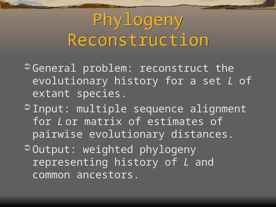
Minimum EvolutionMinimum Evolution Developed by Rzhetsky and Nei (1992) as a
modification of the OLS method For each topology ,
Define function l assigning OLS lengths to edges of
Define size of tree
Choose minimizing l()
( )
( ) ( )e E
l l e
T
T
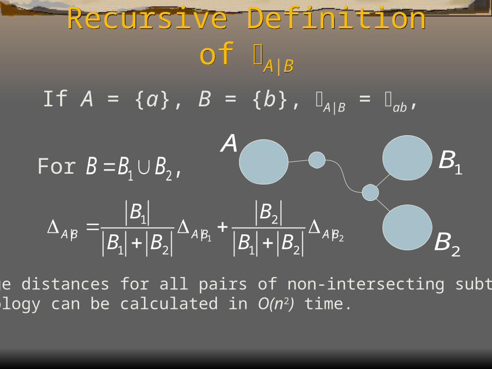
Recursive Definition of A|BRecursive Definition of A|B
If A = {a}, B = {b}, A|B = ab,
1 2
1 2| | |
1 2 1 2A B A B A B
B B
B B B B
All average distances for all pairs of non-intersecting subtrees of a given topology can be calculated in O(n2) time.
For 1 2 ,B B B 1B
2B
A

External OLS Edge Length Function
External OLS Edge Length Function
If e is the edge connecting the leaf i to thesubtrees A and B,
| | |
1( )
2 Ai B i A Bl e
e
B
A
i

Internal OLS Edge Length Function
Internal OLS Edge Length Function
The length of the edge e is (Vach, 1988)
eA C
DB
| | | | | |
1( ) ( ) (1 )( ) ( )
2 A C B D A D B C A B B Cl e
where| || | | || |
.(| | | |)(| | | |)
A D B C
A B C D
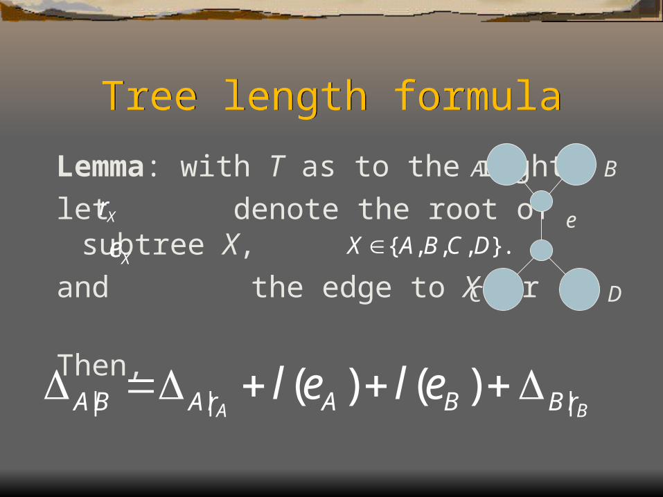
Tree length formulaTree length formula
Lemma: with T as to the right,let denote the root of subtree X,and the edge to X for Then, C
e
A
D
B
Xr
{ , , , }.X A B C D
| | |( ) ( )A BA B A r A B B rl e l e
Xe
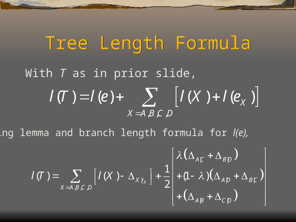
Tree Length FormulaTree Length Formula
With T as in prior slide,
| |
| | |, , ,
| |
1( ) ( ) (1 )
2X
AC B D
X r A D B CX A B C D
A B C D
l T l X
, , ,
( ) ( ) ( ) ( )XX A B C D
l T l e l X l e
Using lemma and branch length formula for l(e),
General approachGeneral approach
To search the space of topologies, we’ll keep in memory two data structures:
Sizes of each subtree of given topologyMatrix of average distances X|Y for X,Y disjoint subtrees in given topology
As we move from one topology to another, we’ll update the matrix, but only as much as needed, in an efficient manner.

Tree Swapping by NNITree Swapping by NNI
C
e
A
D
B
NNI swapping is a basic step in topology building and searching
A
D
C
B
e

Tree Length FormulaTree Length Formula
With T as in prior slide,
| |
| | |, , ,
| |
1( ) ( ) (1 )
2X
AC B D
X r A D B CX A B C D
A B C D
l T l X
, , ,
( ) ( ) ( ) ( )XX A B C D
l T l e l X l e
Using lemma and branch length formula for l(e),
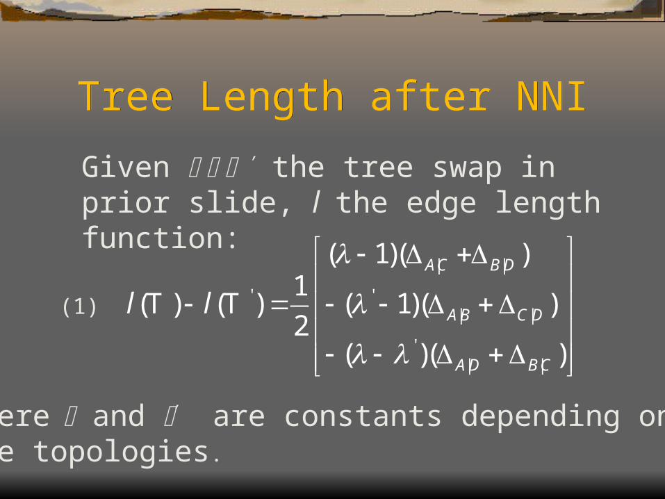
Tree Length after NNITree Length after NNI
Given ’ the tree swap in prior slide, l the edge length function:
| |
' '| |
'| |
( 1)( )1
( ) ( ) ( 1)( )2
( )( )
AC B D
A B C D
A D B C
l l
T T
where and ’ are constants depending on the topologies.
(1)
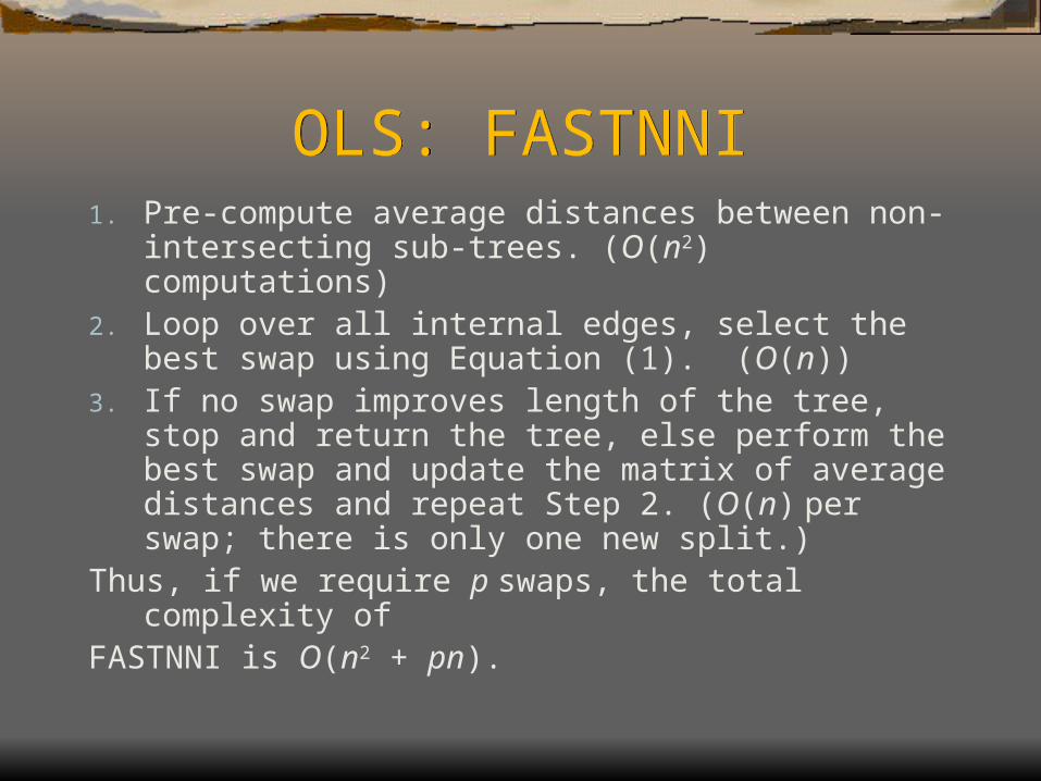
OLS: FASTNNIOLS: FASTNNI1. Pre-compute average distances between non-
intersecting sub-trees. (O(n2) computations)2. Loop over all internal edges, select the best swap
using Equation (1). (O(n))3. If no swap improves length of the tree, stop and return
the tree, else perform the best swap and update the matrix of average distances and repeat Step 2. (O(n) per swap; there is only one new split.)
Thus, if we require p swaps, the total complexity ofFASTNNI is O(n2 + pn).

Balanced Minimum Evolution
Balanced Minimum Evolution
Gascuel (2000) observed that the OLS/ME method was weaker than NJ in approximating the correct topology.
Pauplin (2000) to simplify tree length computation proposed to use a “balanced” version of Minimum Evolution, weighting each sub-tree equally when calculating averages: if A and B are sub-trees of , with
1 2| | |
1 1
2 2A B A B A B T T T
1 2 ,B B B
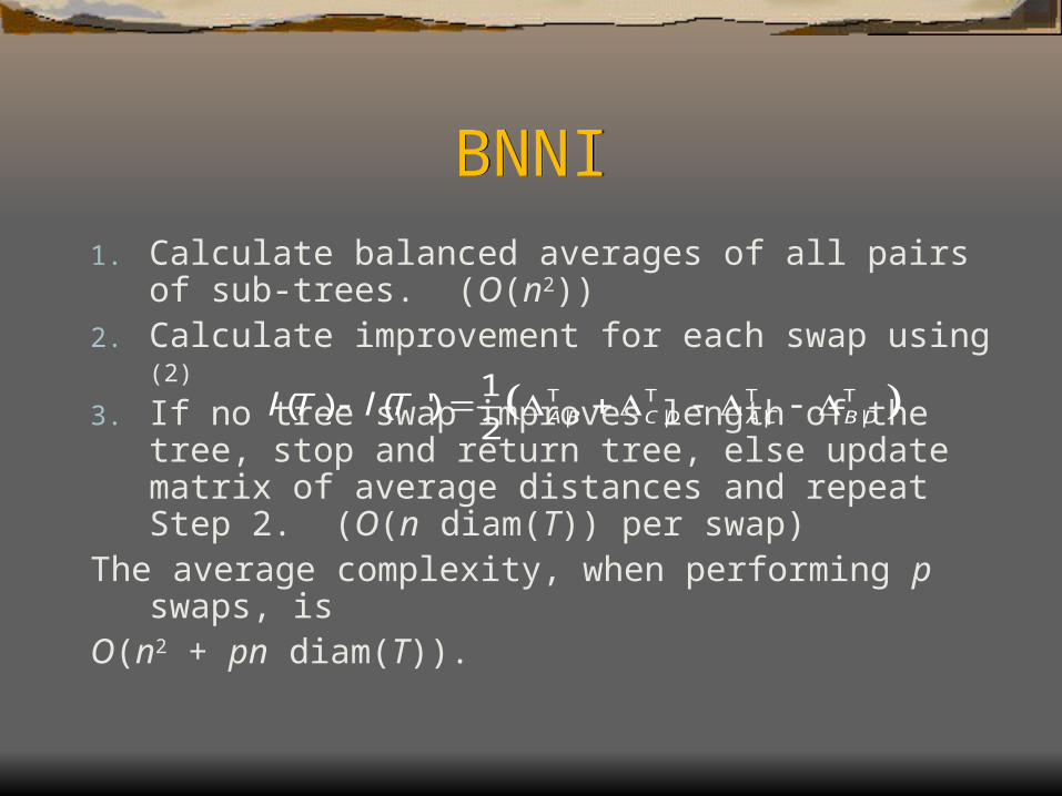
BNNIBNNI
1. Calculate balanced averages of all pairs of sub-trees. (O(n2))
2. Calculate improvement for each swap using (2)
3. If no tree swap improves length of the tree, stop and return tree, else update matrix of average distances and repeat Step 2. (O(n diam(T)) per swap)
The average complexity, when performing p swaps, isO(n2 + pn diam(T)).
| | | |
1( ) ( ')
2 A B C D A C B Dl T l T T T T T

Updating Subtree Averages
Updating Subtree Averages
e
C
DB
y
xX
A
T
Y
Q: How many recalculations?
If we perform the B-C tree swap, then we must recalculate |
TX Y
...X AHere, B C D Y ...and
Typical values for diam(T):
Yule-Harding distribution:
Uniform distribution:
(log )O n
O n
(Hint: you can count (x,y) pairs).
A: O(n diam(T))

Building trees from scratchBuilding trees from scratch
We have NNI algorithms for OLS and balanced branch lengths. But what if we
have no initial topology for NNIs?
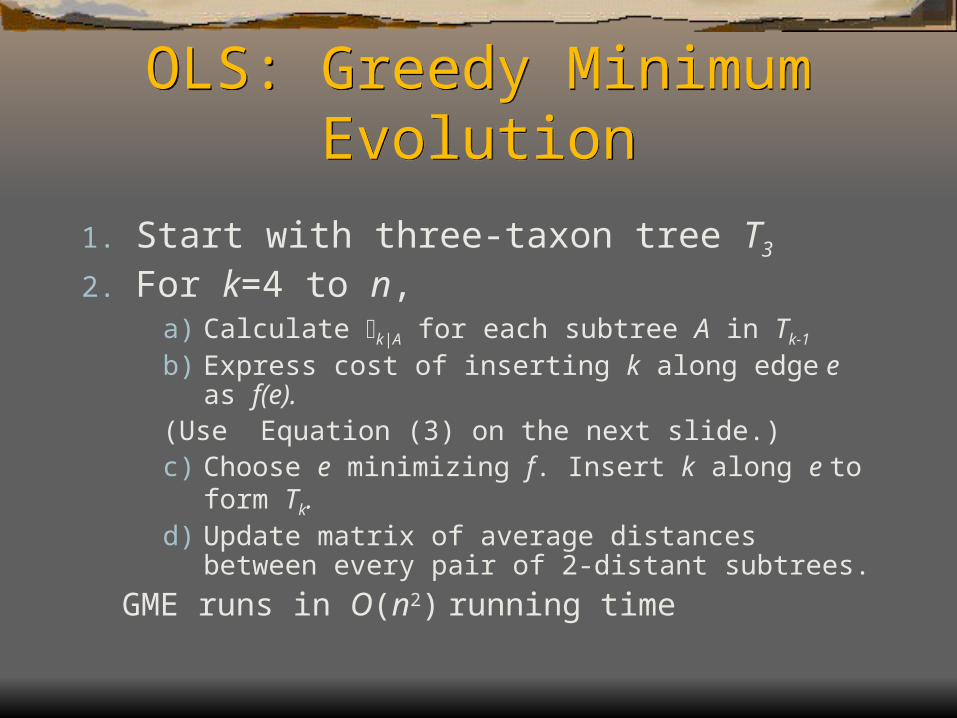
OLS: Greedy Minimum Evolution
OLS: Greedy Minimum Evolution
1. Start with three-taxon tree T3
2. For k=4 to n, a) Calculate k|A for each subtree A in Tk-1
b) Express cost of inserting k along edge e as f(e). (Use Equation (3) on the next slide.)c) Choose e minimizing f. Insert k along e to form Tk.d) Update matrix of average distances between every pair
of 2-distant subtrees.GME runs in O(n2) running time
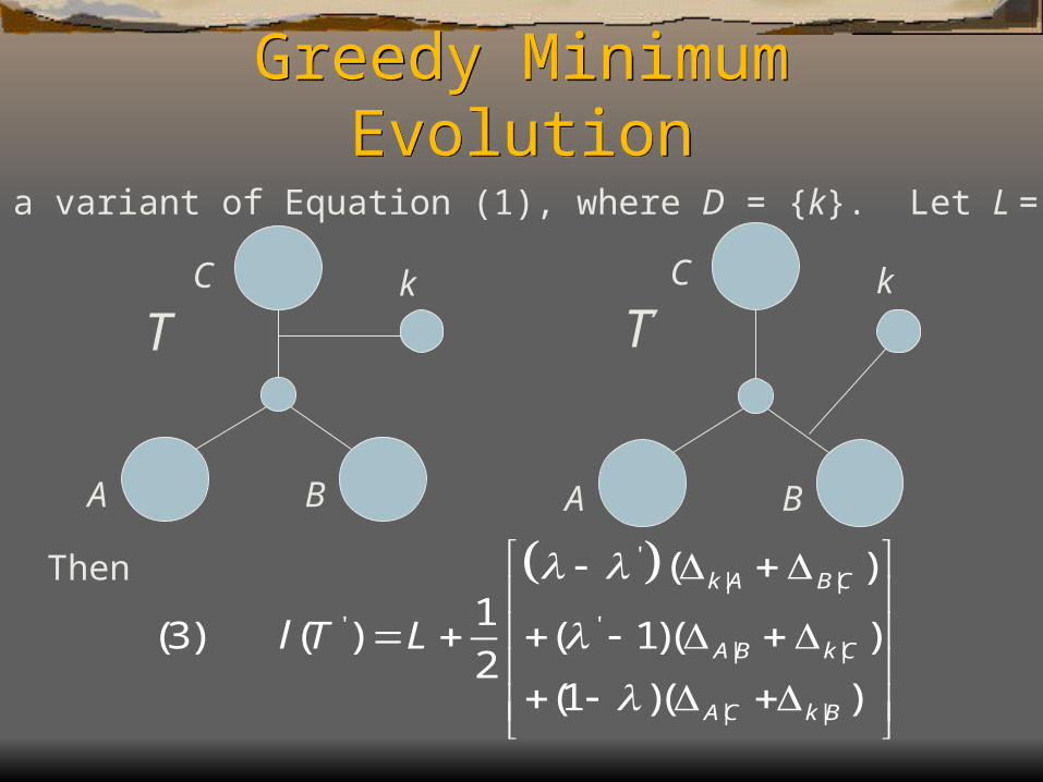
Greedy Minimum Evolution
Greedy Minimum Evolution
C
A B
k
T C
A B
k
T’
' | |
' '| |
| |
( )1
(3) ( ) ( 1)( )2
(1 )( )
k A B C
A B k C
A C k B
l T L
Then
We use a variant of Equation (1), where D = {k}. Let L = l(T).

Balanced Minimum Evolution
Balanced Minimum Evolution
Same as GME,except:2. (modifications)
d) Calculate balanced average distances instead of ordinary average distances
e) Use = ½ to find weights for insertion pointsf) Must keep average distances for all pairs of sub-
trees.
BME runs in O(n2 diam(T)) running time.

SimulationsSimulations Created 24- and 96-taxon trees, 2000 per each
size, Yule-Harding process ( molecular clock). Edge lengths multiplied by (1.0 + X), where X is
exponentially distributed. Generated trees with three rates of evolution SeqGen used to generate sequences for each
tree and rate (12,000 in all) DNADIST used to calculate distance matrices
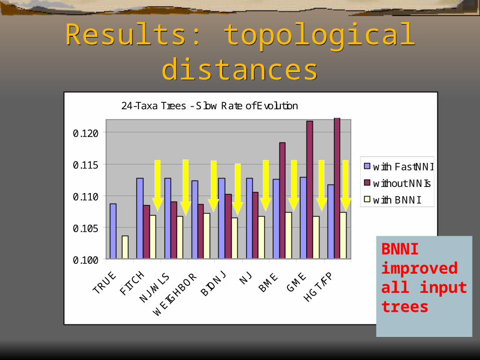
Results: topological distances
Results: topological distances
0.100
0.105
0.110
0.115
0.120
TRUE
FITCH
NJ/W
LS
WEIG
HBOR
BIONJ
NJBM
EGM
E
HGT/
FP
with FastNNI
without NNIs
with BNNI
24-Taxa Trees - Slow Rate of Evolution
BNNI improvedall input trees
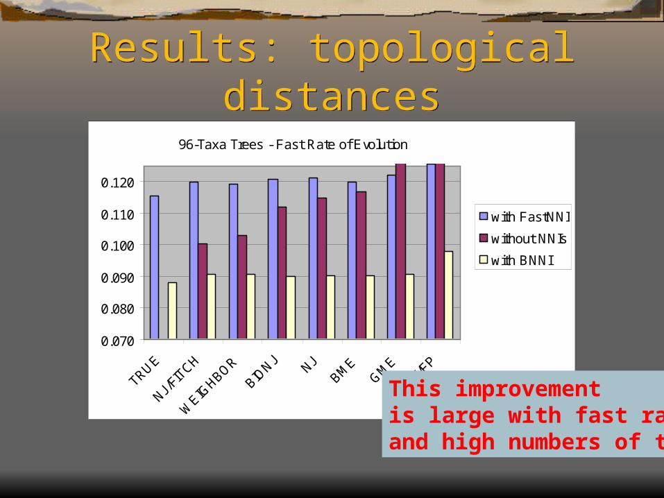
Results: topological distances
Results: topological distances
0.070
0.080
0.090
0.100
0.110
0.120
TRUE
NJ/FI
TCH
WEIG
HBOR
BIONJ
NJBM
EGM
E
HGT/
FP
with FastNNI
without NNIs
with BNNI
96-Taxa Trees - Fast Rate of Evolution
This improvementis large with fast rates and high numbers of taxa
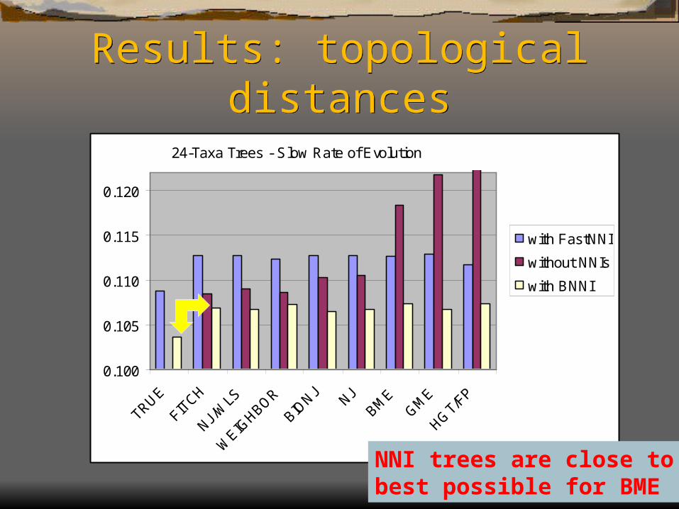
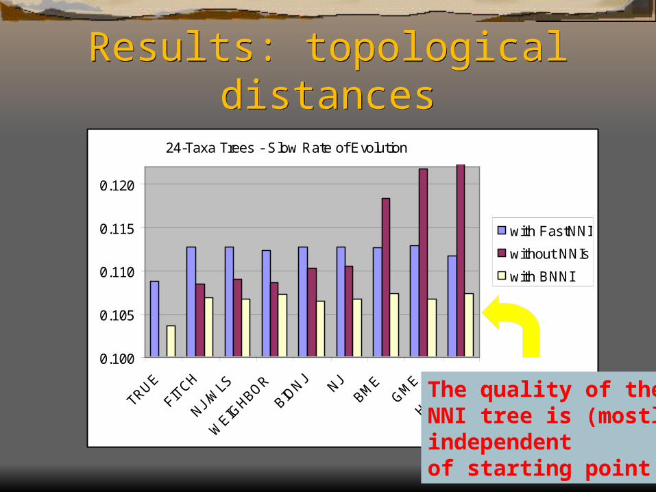
Results: topological distances
Results: topological distances
0.100
0.105
0.110
0.115
0.120
TRUE
FITCH
NJ/W
LS
WEIG
HBOR
BIONJ
NJBM
EGM
E
HGT/
FP
with FastNNI
without NNIs
with BNNI
24-Taxa Trees - Slow Rate of Evolution
NNI trees are close to the best possible for BME
Results: topological distances
Results: topological distances
0.100
0.105
0.110
0.115
0.120
TRUE
FITCH
NJ/W
LS
WEIG
HBOR
BIONJ
NJBM
EGM
E
HGT/
FP
with FastNNI
without NNIs
with BNNI
24-Taxa Trees - Slow Rate of Evolution
The quality of theNNI tree is (mostly)independentof starting point

Results: topological distances
Results: topological distances
0.17
0.175
0.18
0.185
0.19
0.195
0.2
with FastNNI
without NNIs
with BNNI
96-Taxa Trees - Slow Rate of Evolution
FASTNNI trees comparable to NJ as n grows to 96
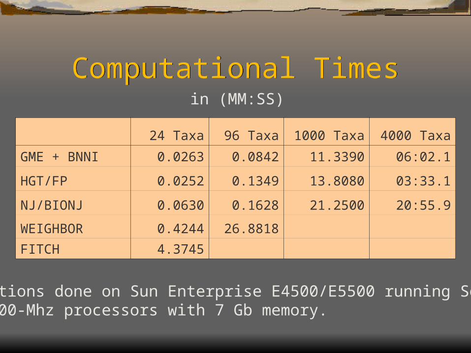
Computational TimesComputational Times
24 Taxa 96 Taxa 1000 Taxa 4000 Taxa
GME + BNNI 0.0263 0.0842 11.3390 06:02.1
HGT/FP 0.0252 0.1349 13.8080 03:33.1
NJ/BIONJ 0.0630 0.1628 21.2500 20:55.9
WEIGHBOR 0.4244 26.8818
FITCH 4.3745
Computations done on Sun Enterprise E4500/E5500 running Solaris 8on 10 400-Mhz processors with 7 Gb memory.
in (MM:SS)
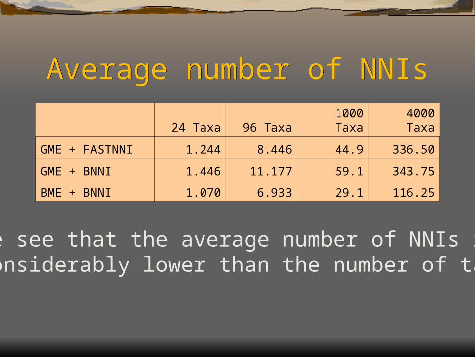
Average number of NNIsAverage number of NNIs
We see that the average number of NNIs is considerably lower than the number of taxa.
24 Taxa 96 Taxa 1000 Taxa 4000 Taxa
GME + FASTNNI 1.244 8.446 44.9 336.50
GME + BNNI 1.446 11.177 59.1 343.75
BME + BNNI 1.070 6.933 29.1 116.25
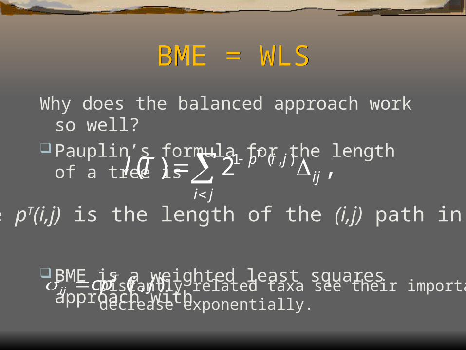
BME = WLSBME = WLS
Why does the balanced approach work so well?Pauplin’s formula for the length of a tree is
BME is a weighted least squares approach with
1 ( , )( ) 2 ,Tp i j
iji j
l T
Where pT(i,j) is the length of the (i,j) path in T.
( , ).Tij cp i j Distantly related taxa see their importance
decrease exponentially.
Bonus featuresBonus features
BME is a consistent method. As observed distances converge to true distances, the true topology becomes the minimum evolution tree.
The BNNI tree has no negative branch lengths. A negative value to the branch length function implies a NNI leading to a smaller tree.
Consistency of Balanced ME
Consistency of Balanced ME
Theorem: Suppose S is a weighted tree, and is a tree topology incompatible with S. Let T be the tree of topology with weights determined by the balanced scheme. Then
l(T) > l(S). Lemma: it suffices to prove the case when S is
a split metric.

Balanced ME consistencyBalanced ME consistency
Basic idea: let l be the tree length function on the space of topologies. We find a sequence of topologies, T=T0, T1, ... Tk=S such that
Each Ti+1 can be reached from Ti via one of two simple topological transformationsl(Ti) > l(Ti+1) for all i.
Proof structure modeled after OLS/ME proof (Rzhetsky and Nei, 1993).
Type I transformationType I transformation
BC C
AAD D
B
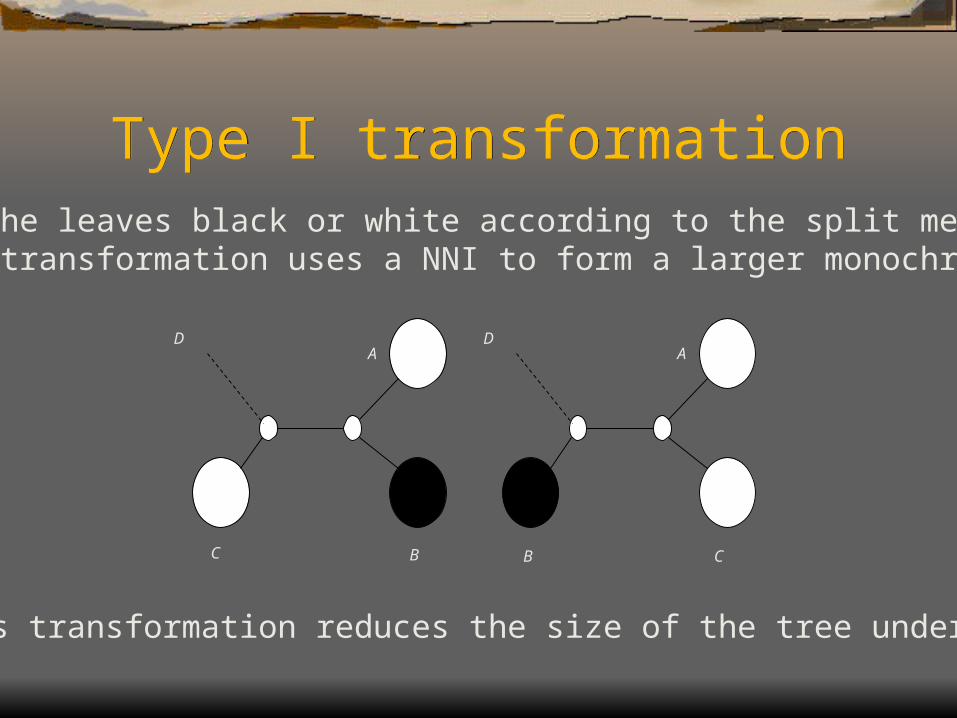
Color the leaves black or white according to the split metric S. A Type I transformation uses a NNI to form a larger monochromatic cluster
This transformation reduces the size of the tree under l

Type II transformationType II transformation
A1
B1
A1
B1
B2 B2
A2
A2
C C
A Type II transformation uses two NNIs to form two monochromaticsubtrees
This transformation also reduces the value of the size of the treeunder l
Positive Branch Lengths after BNNI
Positive Branch Lengths after BNNI
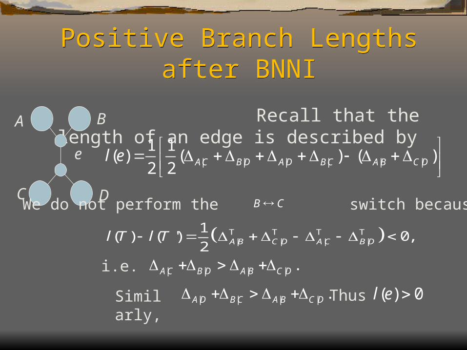
Recall that the length of an edge is described by
| | | | | |
1 1( ) ( ) ( )
2 2 AC B D A D B C A B C Dl e
| | | |
1( ) ( ') 0,
2 A B C D A C B Dl T l T T T T T
C
e
A
D
B
We do not perform the switch becauseB C
i.e. | | | | .A C B D A B C D
Similarly, | | | | .A D B C A B C D Thus ( ) 0l e
ConclusionsConclusions BME + BNNI runs in O((n2 + pn) diam(T)), outputs
trees comparable to (better than) FITCH, Weighbor, BioNJ, or NJ.
FastME is faster than NJ or its variants. BNNI consistently improved output trees in all settings,
even when WLS/Fitch trees were input. BNNI outputs tree without negative branch lengths. FASTME software available at
http://www.ncbi.nlm.nih.gov/CBBResearch/Desper/FastME.html or http://www.lirmm.fr/~w3ifa/MAAS/.