Embed Size (px)
Citation preview

Reference Governor
1

• Reference governor is an add-on safety supervisor for the
existing/legacy controllers
• Monitors and modifies commands if necessary to ensure
constraints are satisfied
Nominal closed-loop system with
an existing/legacy controller
2
Reference Governor
𝑡 ⋅ 𝑇𝑠
Basic idea: Compute 𝑣(𝑡) so that if constantly applied it would not lead to constraint violations
3
Reference Governor

Basic idea: Compute 𝑣(𝑡) so that if constantly applied it would not lead to constraint violations
𝑡 ⋅ 𝑇𝑠
4
Reference Governor
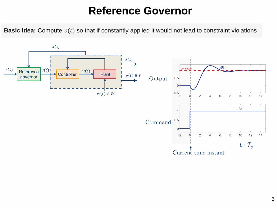
Basic idea: Compute 𝑣(𝑡) so that if constantly applied it would not lead to constraint violations
𝑡 ⋅ 𝑇𝑠
5
y(t)
Reference Governor
Basic idea: Compute 𝑣(𝑡) so that if constantly applied it would not lead to constraint violations
𝑡 ⋅ 𝑇𝑠
6
v(t+𝑘)=
y(t)
Reference Governor

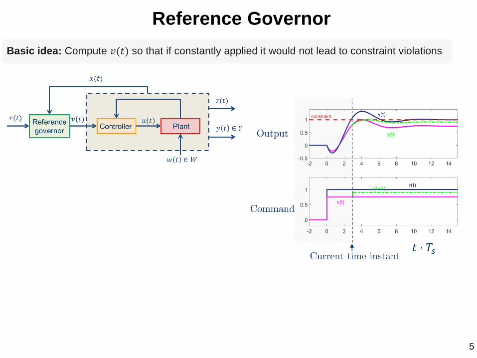
Basic idea: Compute 𝑣(𝑡) so that if constantly applied it would not lead to constraint violations
𝑡 ⋅ 𝑇𝑠
7
v(t+𝑘)=
y(t)
v(t)
Reference Governor

Basic idea: Compute 𝑣(𝑡) so that if constantly applied it would not lead to constraint violations
𝑡 ⋅ 𝑇𝑠
8
v(t+𝑘)=
y(t)
v(t)
Reference Governor

EXPERIMENTS Plant: Inverted Pendulum
Control Law: Linear Quadratic Regulator
LQR𝑢
𝑥
𝑣
𝑟
𝑟
𝑣 𝑣
9Slides from 2014 IEEE CDC Workshop by E. Garone, S. Di Cairano, and I.V. Kolmanovsky

EXPERIMENTS Plant: Inverted Pendulum
Control Law: Linear Quadratic Regulator
𝑟
LQR𝑢
𝑥
RG
𝑟𝑣
𝑣
10Slides from 2014 IEEE CDC Workshop by E. Garone, S. Di Cairano, and I.V. Kolmanovsky
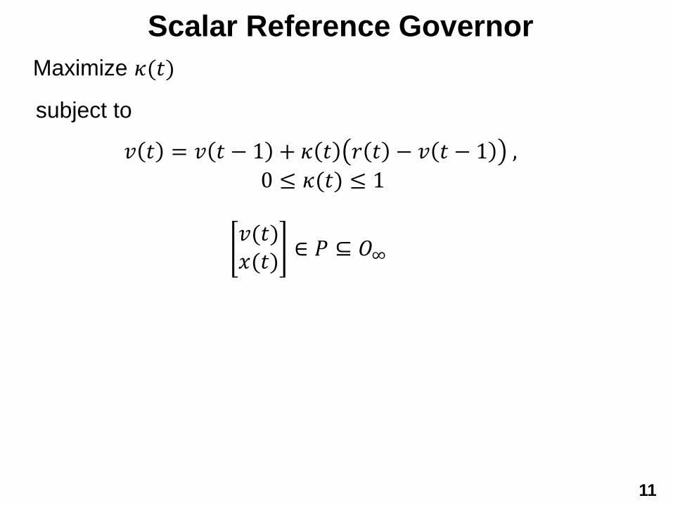
subject to
Maximize 𝜅(𝑡)
𝑣(𝑡)𝑥(𝑡)
∈ 𝑃 ⊆ 𝑂∞
𝑣 𝑡 = 𝑣 𝑡 − 1 + 𝜅 𝑡 𝑟 𝑡 − 𝑣 𝑡 − 1 ,
0 ≤ 𝜅(𝑡) ≤ 1
11
Scalar Reference Governor

• 𝑂∞ is the set of safe pairs of initial states, 𝑥 0 , and
constant commands, 𝑣 𝑡 ≡ 𝑣, which do not cause
subsequent constraint violation
𝑥 𝑡 + 1 = 𝐴𝑥 𝑡 + 𝐵𝑣, 𝑦 𝑡 = 𝐶𝑥 𝑡 + 𝐷𝑣 ∈ 𝑌 ⇒
𝑂∞ = ሼ 𝑣, 𝑥(0) : 𝐶𝐴𝑡𝑥(0) + 𝐶 𝐼 − 𝐴𝑡 𝐼 − 𝐴 −1𝐵𝑣 + 𝐷𝑣 ∈ 𝑌,𝑡 = 0,1,⋯ ,∞ }
• Example: For asymptotically stable observable linear system:
12
Safe Set

13
• Finitely determined inner approximation is obtained by
slightly tightening the “steady-state” constraints
෨𝑂∞ = ሼ 𝑣, 𝑥 0 : (𝐶 𝐼 − 𝐴 −1𝐵 + 𝐷)𝑣 ∈ 1 − 휀 𝑌, 𝐶𝐴𝑡𝑥 0 + 𝐶 𝐼 − 𝐴𝑡 𝐼 − 𝐴 −1𝐵 + 𝐷𝑣 ∈ 𝑌,𝑡 = 0,1,⋯ , 𝑡∗} ⊂ 𝑂∞
Implementation based on subsets

14
• If the constraint set is polyhedral, then ෨𝑂∞ is polyhedral
Safe Sets
𝑌 = 𝑦:𝐻𝑦 ≤ ℎ ⇒
෨𝑂∞ = 𝑣, 𝑥 0 :
𝐻𝐶 𝐼 − 𝐴 −1𝐵 + 𝐷 0𝐻𝐷
𝐻𝐶𝐵 + 𝐻𝐷𝐻𝐶𝐻𝐶𝐴
⋮𝐻𝐶 𝐼 − 𝐴𝑘 𝐼 − 𝐴 −1𝐵 + 𝐻𝐷
⋮
⋮𝐻𝐶𝐴𝑘
⋮
𝑣𝑥(0) ≤
1 − 휀 ℎℎℎ⋮ℎ⋮
• Redundant and “almost redundant” inequality constraints are
eliminated while remaining constraints are tightened to obtain
a simply represented 𝑃 ⊆ ෨𝑂∞
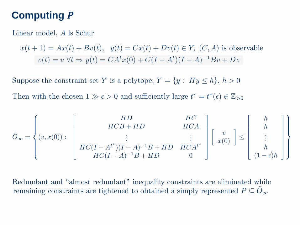
Computing 𝑷

Computing 𝜿

17
Example
Model:
𝑥1 𝑡 + 1 = 𝑥1 𝑡 + 0.1𝑥2 𝑡 ,𝑥2(𝑡 + 1) = 𝑥2 𝑡 + 0.1𝑢(𝑡)
Constraints:
|𝑥1| ≤ 1,|𝑥2| ≤ 0.1,
|𝑢| ≤ 0.1
Nominal closed-loop:
𝑢 = −0.917 𝑥1 − 𝑟 − 1.636𝑥2,
Reference command
𝑟 𝑡 = 0.5.
0 20 40 60 80-0.1
0
0.1
0.2
0.3
0.4
0.5
t
x1
x2
u
Response without reference governor

18
Example (cont’d)
𝑢 = −0.917 𝑥1 − 𝑣 𝑡 − 1.636𝑥2 , 𝑣(𝑡) = 𝑅𝐺(𝑣 𝑡 − 1 , 𝑥 𝑡 )
Response with reference governor

19
Example (cont’d)
Cross-sections of 𝑃 = ෨𝑂∞ :

1 DOF spacecraft with flexible appendage
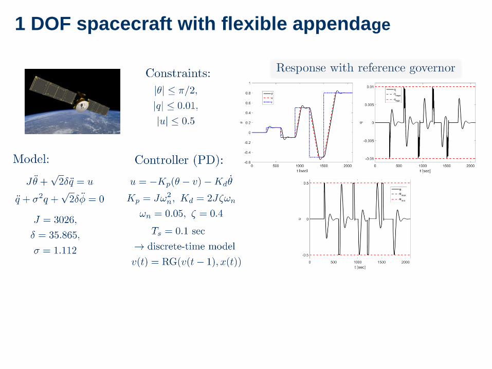
1 DOF spacecraft with flexible appendage
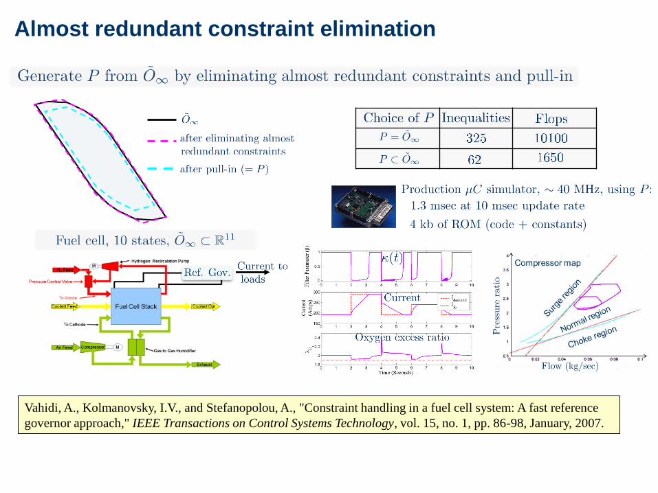
Almost redundant constraint elimination
Vahidi, A., Kolmanovsky, I.V., and Stefanopolou, A., "Constraint handling in a fuel cell system: A fast reference
governor approach," IEEE Transactions on Control Systems Technology, vol. 15, no. 1, pp. 86-98, January, 2007.

More general sets 𝑷, nonlinear systems…

Scalar reference governor

Using 𝑷 without actually computing it
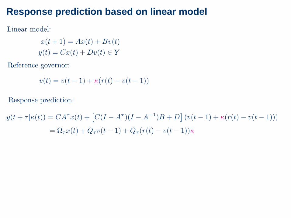
Response prediction based on linear model
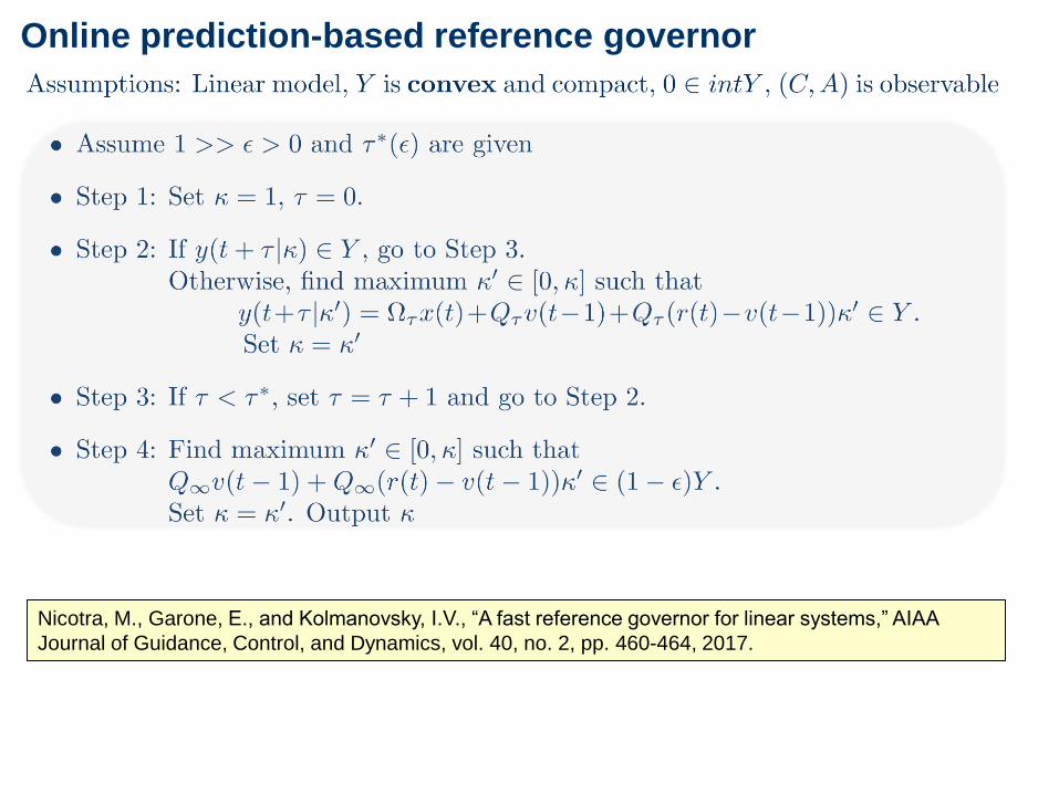
Online prediction-based reference governor
Nicotra, M., Garone, E., and Kolmanovsky, I.V., “A fast reference governor for linear systems,” AIAA
Journal of Guidance, Control, and Dynamics, vol. 40, no. 2, pp. 460-464, 2017.

• Linear and nonlinear systems with set-bounded
disturbances and parameter uncertainties can be treated
• Feasibility at initial time implies constraint adherence and
recursive feasibility for all future times
• Finite-time convergence of 𝑣(𝑡) to 𝑟(𝑡) or nearest steady-
state feasible value for constant 𝑟(𝑡)
• Similar convergence results for ``nearly constant’’ and
slowly-varying 𝑟(𝑡)
• Enlarged constrained domain of attraction
28
Remarks on existing theory

Survey paper

Reference governor extensions

Reference governor extensions

Reference governor extensions

Implementing Linear
Design on a
Nonlinear System
33

Adopting linear design to a nonlinear system
12/15/2014
• Consider a disturbance-free nonlinear system
𝛿𝑥 𝑡 + 1 = 𝐴𝛿𝑥 𝑡 + 𝐵𝛿𝑣(𝑡) ∈ 𝑌
𝛿𝑥 𝑡 = 𝑥 − 𝑥𝑜𝑝,
𝛿𝑣 𝑡 = 𝑣 − 𝑣𝑜𝑝,
𝑓 𝑥𝑜𝑝, 𝑣𝑜𝑝 = 0
𝑦𝑙𝑖𝑛 𝑡 = 𝐶 𝛿𝑥 𝑡 + 𝐷 𝛿𝑣 𝑡
• Let a linearization of the nonlinear model at an operating
point (𝑥𝑜𝑝, 𝑣𝑜𝑝, 𝑦𝑜𝑝) be given by
𝑥 𝑡 + 1 = 𝑓 𝑥 𝑡 , 𝑣 𝑡
𝑦𝑛𝑜𝑛𝑙 𝑡 = 𝑔 𝑥 𝑡 , 𝑣 𝑡 ∈ 𝑌
34
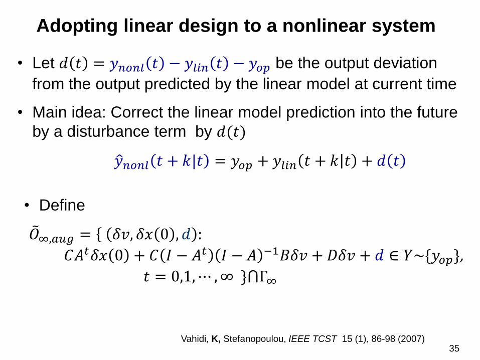
Adopting linear design to a nonlinear system
• Main idea: Correct the linear model prediction into the future
by a disturbance term by 𝑑(𝑡)
ො𝑦𝑛𝑜𝑛𝑙 𝑡 + 𝑘|𝑡 = 𝑦𝑜𝑝 + 𝑦𝑙𝑖𝑛 𝑡 + 𝑘 𝑡 + 𝑑 𝑡
෨𝑂∞,𝑎𝑢𝑔 = ሼ 𝛿𝑣, 𝛿𝑥 0 , 𝑑 :
𝐶𝐴𝑡𝛿𝑥 0 + 𝐶 𝐼 − 𝐴𝑡 𝐼 − 𝐴 −1𝐵𝛿𝑣 + 𝐷𝛿𝑣 + 𝑑 ∈ 𝑌~ሼ𝑦𝑜𝑝},𝑡 = 0,1,⋯ ,∞ }⋂Γ∞
Vahidi, K, Stefanopoulou, IEEE TCST 15 (1), 86-98 (2007)
• Let 𝑑 𝑡 = 𝑦𝑛𝑜𝑛𝑙 𝑡 − 𝑦𝑙𝑖𝑛 𝑡 − 𝑦𝑜𝑝 be the output deviation
from the output predicted by the linear model at current time
• Define
35

Adopting linear design to a nonlinear system
𝑣 𝑡 − 1 + 𝛽 𝑡 𝑟 𝑡 − 𝑣 𝑡 − 𝑣𝑜𝑝𝛿𝑥(𝑡)𝑑(𝑡)
∈ ෨𝑂∞,𝑎𝑢𝑔
𝛽 𝑡 → max 𝑠𝑢𝑏𝑗𝑒𝑐𝑡 𝑡𝑜 0 ≤ 𝛽 𝑡 ≤ 1
• Reference governor logic:
𝑑 𝑡 = 𝑦𝑛𝑜𝑛𝑙𝑖𝑛 𝑡 − 𝑦𝑙𝑖𝑛 𝑡 − 𝑦𝑜𝑝
𝑎𝑛𝑑
36

Discussion
• The proposed technique is motivated by a similar scheme in
MPC
• It is heuristic but has been shown to work well in several
applications
• The study of its theoretical properties remains an open
research problem
• Extensions to command governor and extended command
governor cases are feasible
37

Controller state and reference governor (CSRG)
Controller PlantCSRG
K. McDonough and I.V. Kolmanovsky, “Controller state and reference governors for discrete-time
linear systems with pointwise-in-time state and control constraints,” Proceedings of 2015 American
Control Conference, Chicago, IL, pp. 3607-3612, 2015.

Gas turbine engine

Command
CSRG modified
command
Fan speed
Constraints
Linear model simulations

• Trim point to trim point transition feasibility is
determined based on set of states that can be
recovered by CSRG
• The actual transitions are controlled by CSRG
Envelope-aware flight management system
Di Donato, P.F.A., Balachandran, S., McDonough, K., Atkins, E., and Kolmanovsky, I.V., “Envelope-
aware flight management for loss of control prevention given rudder jam,” AIAA Journal of Guidance,
Control, and Dynamics, vol. 40, pp. 1027-1041, 2017.
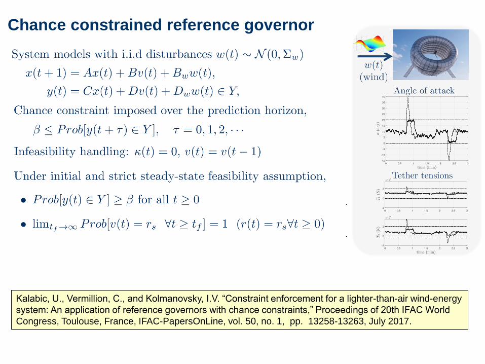
Chance constrained reference governor
Kalabic, U., Vermillion, C., and Kolmanovsky, I.V. “Constraint enforcement for a lighter-than-air wind-energy
system: An application of reference governors with chance constraints,” Proceedings of 20th IFAC World
Congress, Toulouse, France, IFAC-PapersOnLine, vol. 50, no. 1, pp. 13258-13263, July 2017.

Formation control
Frey, G., Petersen, C., Leve, F., Garone, E., Kolmanovsky, I.V. and Girard, A., “Parameter governors for
coordinated control of n-spacecraft formations,” AIAA Journal of Guidance, Control, and Dynamics, vol. 40,
no. 11, pp. 3020-3025, November, 2017.

Concluding remarks
Controller PlantReference
governor
• Augment rather than replace nominal controller
• Inactive if no danger of constraint violation
• Easy to implement / fast online computations
• Special properties
• Much room for future research and applications

BACKUP SLIDES
45

The Extended Command
Governor (ECG)
46
Agenda
• Extended Command Governor (ECG)
• Design of ancillary dynamical system
• Response properties
• Interpretation as a form of Model Predictive Controller (MPC)
• Application examples
• Command governor and vector reference governor
47
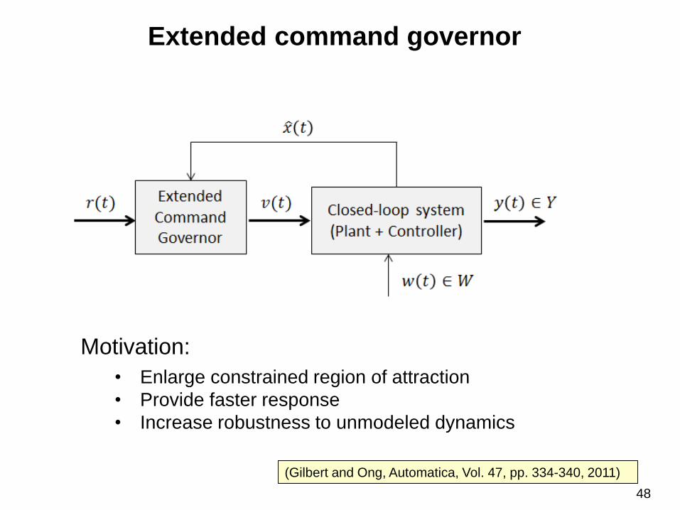
Extended command governor
(Gilbert and Ong, Automatica, Vol. 47, pp. 334-340, 2011)
Motivation:
• Enlarge constrained region of attraction
• Provide faster response
• Increase robustness to unmodeled dynamics
48

Extended command governor
ҧ𝑥 𝑡 + 1 = ҧ𝐴 ҧ𝑥 𝑡
𝜌 𝑡 + 1 = 𝜌 𝑡
𝑥 𝑡 + 1 = 𝐴𝑥 𝑡 + 𝐵𝑣 𝑡
𝑦 𝑡 = 𝐶𝑥 𝑡 + 𝐷𝑣 𝑡 ∈ 𝑌
• Auxiliary “command generating” subsystem:
• System:
𝑣 𝑡 = 𝜌 𝑡 + ҧ𝐶 ҧ𝑥 𝑡
• Requirement: ҧ𝐴 is asymptotically stable (Schur)

Auxiliary command generator
𝜌(0)
𝑣 𝑡 = ҧ𝐶 ҧ𝐴𝑡 𝑥 0 + 𝜌(0)
0 𝑡
ҧ𝑥 𝑡 + 1 = ҧ𝐴 ҧ𝑥 𝑡
𝜌 𝑡 + 1 = 𝜌 𝑡
𝑣 𝑡 = 𝜌 𝑡 + ҧ𝐶 ҧ𝑥 𝑡
𝑣 𝑡
• Auxiliary “command generating” subsystem:
50

Augmented system
ҧ𝑥 𝑡 + 1 = ҧ𝐴 ҧ𝑥 𝑡
𝜌 𝑡 + 1 = 𝜌 𝑡
𝑥 𝑡 + 1 = 𝐴𝑥 𝑡 + 𝐵𝑣 𝑡
𝑦 𝑡 = 𝐶𝑥 𝑡 + 𝐷𝑣 𝑡 ∈ 𝑌
𝑣 𝑡 = 𝜌 𝑡 + ҧ𝐶 ҧ𝑥 𝑡
• Combined system:
• Constraints:
51

Augmented system
𝑦 𝑡 = 𝐶𝑥 𝑡 + 𝐷𝑣 𝑡 ∈ 𝑌
• Augmented system with constraints
ҧ𝑥(𝑡 + 1)𝑥(𝑡 + 1)
= 𝐴𝑎ҧ𝑥(𝑡)𝑥(𝑡)
+ 𝐵𝑎 𝜌 𝑡
𝐴𝑎 =ҧ𝐴 0
𝐵 ҧ𝐶 𝐴, 𝐵𝑎 =
0𝐵
𝐶𝑎 = 𝐷 ҧ𝐶 𝐶 𝐷𝑎 = 𝐷
52

Strictly steady-state admissible commands
• Set Γ∞ of steady-state admissible constant references:
Γ∞ = ሼ 𝜌 0 , ҧ𝑥 0 , 𝑥(0) : 𝜌(0) ∈ ℛ}
• Tightened set of steady-state feasible commands:
𝑟 ∈ ℛ ⇒ 𝐻𝑟 ∈ 1 − 𝜖 𝑌
• Static gain 𝐻 = 𝐶 𝐼 − 𝐴 −1𝐵 + 𝐷
0 ∈ 𝑖𝑛𝑡 𝑌, 𝑌 is compact, 0 < 𝜖 < 1
53

The set 𝑶∞
𝑂∞ = ሼ 𝜌 0 , ҧ𝑥 0 , 𝑥(0) : 𝑦(𝑡) ∈ 𝑌, 𝑡 = 0,1,⋯ ,∞}
• Safe set
54

The set ෩𝑶∞
• Safe set is tightened in steady-state
෨𝑂∞ = 𝑂∞ ⋂Γ∞
• Properties (under suitable assumptions):
• 𝑟 ∈ ℛ ⇒ (𝑟, 0, 𝑥𝑠𝑠 𝑟 ) = (𝑟, 0, 𝐻𝑟) ∈ 𝑖𝑛𝑡 𝑂∞
• ෨𝑂∞ is positively invariant for augmented system
• ෨𝑂∞ is finitely-determined
55

• Suppose 𝑌 is a polytope: 𝑌 = ሼ𝑦: Λy ≤ 𝜆}
𝐻𝜌,𝑡 𝜌 + 𝐻 ҧ𝑥,𝑡 ҧ𝑥 0 +𝐻𝑥,𝑡 𝑥 0 ≤ 𝜆
𝐻∞𝜌 ≤ (1 − 𝜖)𝜆
𝐻 ҧ𝑥,𝑡, 𝐻𝑥,𝑡 = Λ𝐶𝑎𝐴𝑎𝑡 ,
𝐻𝜌,𝑡 = Λ(𝐶𝑎 𝐼 − 𝐴𝑎𝑡 𝐼 − 𝐴𝑎
−1𝐵𝑎 + 𝐷𝑎)
𝐻∞ = Λ(𝐶𝑎 𝐼 − 𝐴𝑎−1𝐵𝑎 + 𝐷𝑎)
The set ෩𝑶∞
• Then ෨𝑂∞ is defined by affine inequalities on 𝜌, ҧ𝑥 0 , 𝑥 0 :
• Consider the disturbance-free case (𝑊 = 0)
• Inequalities for all 𝑡 sufficiently large (𝑡 ≥ 𝑡∗) are redundant
and need not be included
(𝑡 = 0,12,⋯ )
(0 < 𝜖 ≪ 1)
56

subject to
𝜌 𝑡 , ҧ𝑥 𝑡 , 𝑥(𝑡) ∈ ෨𝑂∞
𝐽 = 𝜌 𝑡 − 𝑟 𝑡𝑇𝑆(𝜌 𝑡 − 𝑟 𝑡 ) + ҧ𝑥 𝑡 𝑇 ҧ𝑆 ҧ𝑥(𝑡) → 𝑚𝑖𝑛𝜌(𝑡), ҧ𝑥(𝑡)
Extended command governor
• Optimization problem:
• Command computation based on ҧ𝑥(𝑡) and 𝜌(𝑡):
𝑣 𝑡 = ҧ𝐶 ҧ𝑥 𝑡 + 𝜌(𝑡)
57

Extended command governor
ҧ𝐴𝑇 ҧ𝑆 ҧ𝐴 − ҧ𝑆 < 0, ҧ𝑆𝑇 = ҧ𝑆 > 0
• Assumption 2: The weight ҧ𝑆 in the cost function must satisfy
• Assumption 1: The weight 𝑆 in the cost function satisfies
𝑆𝑇 = 𝑆 > 0
• Observation: If 𝜌 𝑡 − 1 , ҧ𝑥(𝑡 − 1) are feasible at time 𝑡 − 1,
then
𝜌 𝑡 = 𝜌 𝑡 − 1 , 𝑥 𝑡 = ҧ𝐴 ҧ𝑥(𝑡 − 1)
are feasible at time 𝑡 and
𝑥𝑇 𝑡 ҧ𝑆 𝑥 𝑡 ≤ ҧ𝑥𝑇 𝑡 − 1 ҧ𝑆 ҧ𝑥(𝑡 − 1)
58
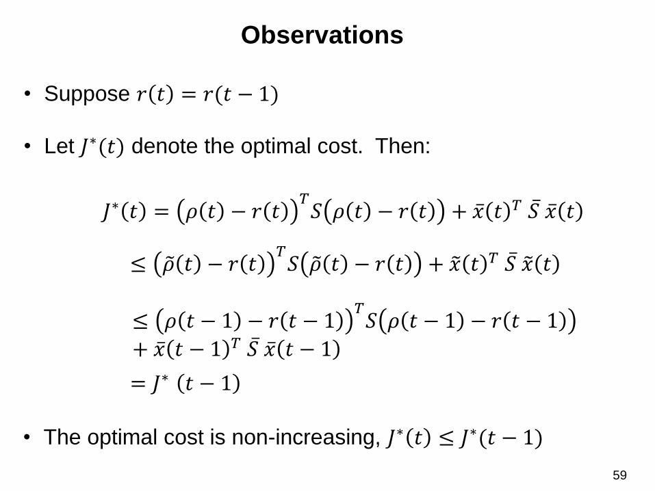
Observations
• Suppose 𝑟 𝑡 = 𝑟(𝑡 − 1)
• Let 𝐽∗(𝑡) denote the optimal cost. Then:
𝐽∗ 𝑡 = 𝜌 𝑡 − 𝑟 𝑡𝑇𝑆 𝜌 𝑡 − 𝑟 𝑡 + ҧ𝑥 𝑡 𝑇 ҧ𝑆 ҧ𝑥 𝑡
= 𝐽∗ 𝑡 − 1
≤ 𝜌 𝑡 − 𝑟 𝑡𝑇𝑆 𝜌 𝑡 − 𝑟 𝑡 + 𝑥 𝑡 𝑇 ҧ𝑆 𝑥 𝑡
≤ 𝜌 𝑡 − 1 − 𝑟 𝑡 − 1𝑇𝑆 𝜌 𝑡 − 1 − 𝑟 𝑡 − 1
+ ҧ𝑥 𝑡 − 1 𝑇 ҧ𝑆 ҧ𝑥 𝑡 − 1
• The optimal cost is non-increasing, 𝐽∗ 𝑡 ≤ 𝐽∗(𝑡 − 1)
59
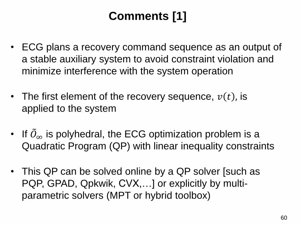
Comments [1]
• ECG plans a recovery command sequence as an output of
a stable auxiliary system to avoid constraint violation and
minimize interference with the system operation
• The first element of the recovery sequence, 𝑣 𝑡 , is
applied to the system
• If ෨𝑂∞ is polyhedral, the ECG optimization problem is a
Quadratic Program (QP) with linear inequality constraints
• This QP can be solved online by a QP solver [such as
PQP, GPAD, Qpkwik, CVX,…] or explicitly by multi-
parametric solvers (MPT or hybrid toolbox)
60

Comments [2]
• ECG achieves large constrained domain of attraction
(= 𝑃𝑟𝑜𝑗𝑥 ෨𝑂∞). It is typically larger than that of RG
• ECG achieves faster response, i.e., faster
convergence of 𝑣(𝑡) to 𝑟, in particular, for systems with
actuator rate limits
• Improved robustness to model uncertainty observed in
simulations
61

Theoretical results
• Suppose a feasible solution exists at time 0 and 𝑟 𝑡 = 𝑟𝑠
for all 𝑡 ≥ 𝑡𝑠. Define 𝑟𝑠∗ = argmin
𝑟∈ℛ𝑟 − 𝑟𝑠
2be the
nearest feasible reference
• Then there exists a 𝑡𝑓 ∈ 𝑍+ such that 𝑣 𝑡 = 𝑟𝑠∗ for all 𝑡 ≥ 𝑡𝑓 .
• Given 𝜖 > 0, there exists a 𝑡𝜖 ∈ 𝑍+ such that
𝑥 𝑡 ∈ 𝐹∞ 𝑟𝑠∗ + 𝜖𝐵𝑛 for all 𝑡 ≥ 𝑡𝜖
(Gilbert and Ong, 2011)
62

Sketch of the proof
• 𝐽∗(𝑡) is monotonically non-increasing, hence
𝐽∗ 𝑡 − 1 − 𝐽∗ 𝑡 → 0
• Using the properties of minimum norm projection on a closed
and convex set, it is shown that
ҧ𝐴 ҧ𝑥 𝑡 − 1 − ҧ𝑥 𝑡ҧ𝑆
2+ 𝜌(𝑡 − 1) − 𝜌 𝑡
𝑆
2≤ 𝐽∗ 𝑡 − 1 − 𝐽∗(𝑡)
• Henceҧ𝐴 ҧ𝑥 𝑡 − 1 − ҧ𝑥 𝑡 → 0
𝜌 𝑡 − 1 − 𝜌 𝑡 → 0 as 𝑡 → ∞
63

Sketch of the proof
• Apply Lemma with
𝑧 = ҧ𝐴 ҧ𝑥 𝑡 − 1 , 𝜌 𝑡 − 1 , 𝑧𝑜𝑝 = ҧ𝑥 𝑡 , 𝜌 𝑡 ,
𝑧𝑠 = 0, 𝑟 , 𝑄 = 𝑑𝑖𝑎𝑔( ҧ𝑆, 𝑆)
64

Sketch of the proof
𝑧𝑜𝑝
𝑧𝑠
𝑧𝑎
𝑏𝑐
𝑎2 + 𝑏2 ≤ 𝑐2 since 𝜃 ≥ 𝜋/2
𝑍
𝜃
⇒ 𝑎2 ≤ 𝑐2 − 𝑏2
65

Sketch of the proof
• Thus ҧ𝑥 𝑡 = ҧ𝐴 ҧ𝑥 𝑡 − 1 + 𝜂(𝑡), and 𝜂 𝑡 → 0 as 𝑡 → ∞.
• Since ҧ𝐴 is Schur, ҧ𝑥 𝑡 → 0.
• Thus 𝑣 𝑡 − 𝑣 𝑡 − 1 → 0 and 𝑥 𝑡 → 𝑥𝑠𝑠 𝑡
• The proof is finalized by strict constraint admissibility in
steady-state. Formally, we demonstrate that for large 𝑡and 휀 > 0 sufficiently small,
𝜌 𝑡 − 휀𝜌 𝑡 −𝑟𝑠
𝜌 𝑡 −𝑟𝑠, ҧ𝑥(𝑡) = 0
are feasible.
• This is only possible if 𝜌 𝑡 = 𝑟𝑠 and hence 𝑣 𝑡 = 𝑟𝑠
66
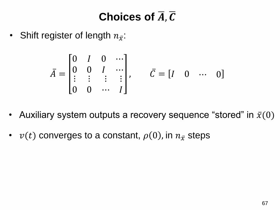
Choices of ഥ𝑨, ഥ𝑪
• Shift register of length 𝑛 ҧ𝑥:
ҧ𝐴 =
0 𝐼0 0
0 ⋯𝐼 ⋯
⋮ ⋮0 0
⋮ ⋮⋯ 𝐼
, ҧ𝐶 = 𝐼 0 ⋯ 0
• Auxiliary system outputs a recovery sequence “stored” in ҧ𝑥(0)
• 𝑣(𝑡) converges to a constant, 𝜌 0 , in 𝑛 ҧ𝑥 steps
67

Example
• Example: 𝑣 ∈ 𝑅1, 𝑛 ҧ𝑥 = 3
• Augmented state
𝑣 𝑛 ҧ𝑥 + 𝑘 = 𝜌 0 , 𝑘 ≥ 0
ҧ𝑥 =ҧ𝑥1ҧ𝑥2ҧ𝑥3
• Generated command sequence:
𝑣 0 = 𝜌 0 + ҧ𝑥1 0 ,𝑣 1 = 𝜌 0 + ҧ𝑥2 0 ,𝑣 2 = 𝜌 0 + ҧ𝑥3 0
68

Choices of ഥ𝑨, ഥ𝑪
• Laguerre Sequence Generator:
ҧ𝐴 =
휀𝐼 𝛽𝐼 −휀𝛽𝐼 휀2𝛽𝐼 ⋯
0 휀𝐼 𝛽𝐼 −휀𝛽𝐼 ⋯00⋮
00⋮
휀𝐼0⋮
𝛽𝐼휀I⋮
⋯⋯⋱
,
ҧ𝐶 = 𝛽 𝐼 −휀I 휀2𝐼 −휀3𝐼 ⋯ −휀 𝑁−1𝐼
where 𝛽 = 1 − 휀2, and 0 ≤ 휀 ≤ 1 is a selectable parameter that
corresponds to the time constant of the fictitious dynamics. Note that
with 휀 = 0, this is the shift register.
(Kalabic et. al., Proc. of 2011 MSC)
69
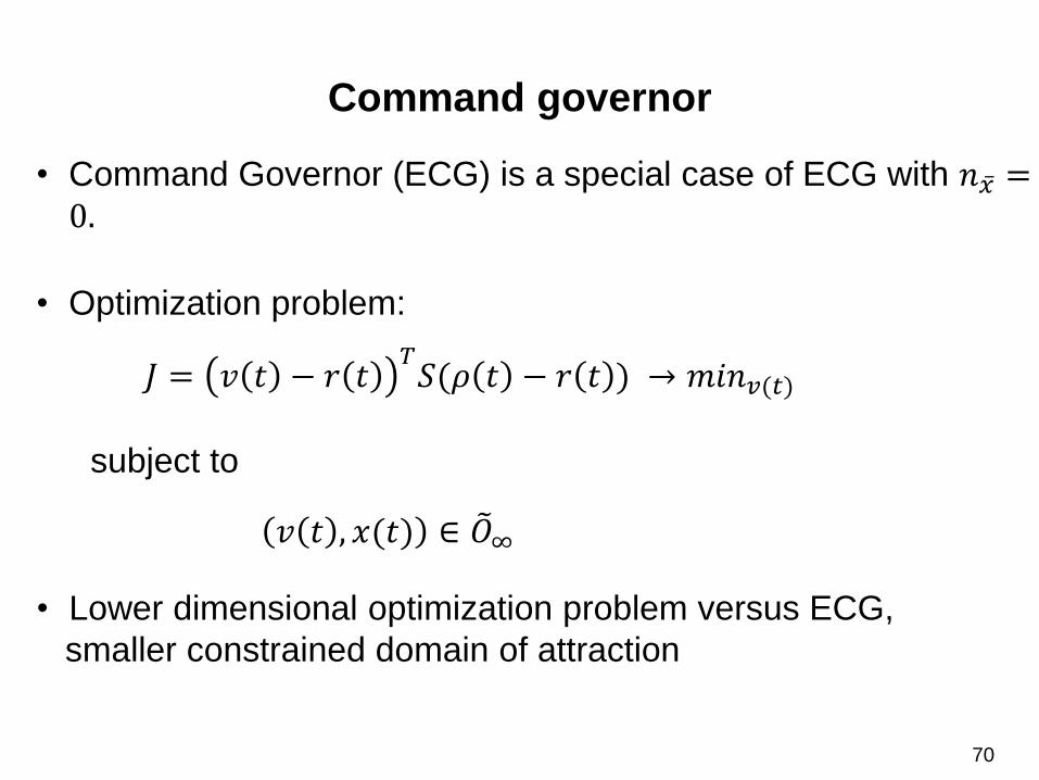
Command governor
subject to
𝑣 𝑡 , 𝑥(𝑡) ∈ ෨𝑂∞
𝐽 = 𝑣 𝑡 − 𝑟 𝑡𝑇𝑆(𝜌 𝑡 − 𝑟 𝑡 ) → 𝑚𝑖𝑛𝑣(𝑡)
• Command Governor (ECG) is a special case of ECG with 𝑛 ҧ𝑥 =0.
• Optimization problem:
• Lower dimensional optimization problem versus ECG,
smaller constrained domain of attraction
70
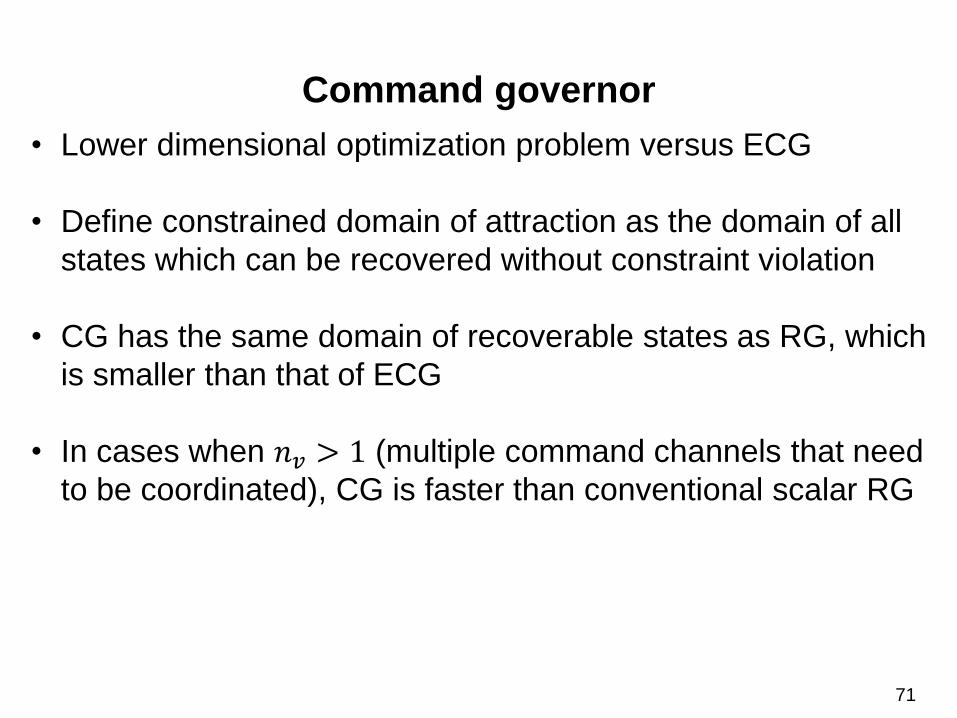
Command governor
• Lower dimensional optimization problem versus ECG
• Define constrained domain of attraction as the domain of all
states which can be recovered without constraint violation
• CG has the same domain of recoverable states as RG, which
is smaller than that of ECG
• In cases when 𝑛𝑣 > 1 (multiple command channels that need
to be coordinated), CG is faster than conventional scalar RG
71

Vector Reference Governor (VRG)
𝑣 𝑡 = 𝑣 𝑡 − 1 + Κ 𝑡 (𝑟 𝑡 − 𝑣 𝑡 − 1 )
Κ 𝑡 =
𝜅1(𝑡) 0 00 ⋱ 00 0 𝜅𝑛𝑣(𝑡)
0 ≤ 𝜅𝑖 𝑡 ≤ 1, 𝑖 = 1,⋯ , 𝑛𝑣
• Vector Reference Governor uses a vector gain to
independently adjust each channel
• Optimization problem: 𝑣 𝑡 − 𝑟 𝑡𝑇𝑆(𝑣 𝑡 − 𝑟 𝑡 ) → min
𝑣 t
subject to 𝑣 𝑡 = 𝑣 𝑡 − 1 + Κ 𝑡 (𝑟 𝑡 − 𝑣 𝑡 − 1 )
𝑣 𝑡 , 𝑥 𝑡 ∈ ෨𝑂∞72

MPC format for ECG
• ECG with the shift register can be re-formulated as a
special variant of MPC controller
• Let 𝑣 𝑡 = 𝜌 𝑡 + 𝑢 𝑡
• Introduce notation commonly used in predictive control
𝑣 𝑡 + 𝑘 𝑡 = 𝜌 𝑡 + 𝑢 𝑡 + 𝑘 𝑡 , 𝑘 = 0,⋯ ,𝑁𝑐 − 1
• Consider the disturbance-free case with 𝑊 = 0
73
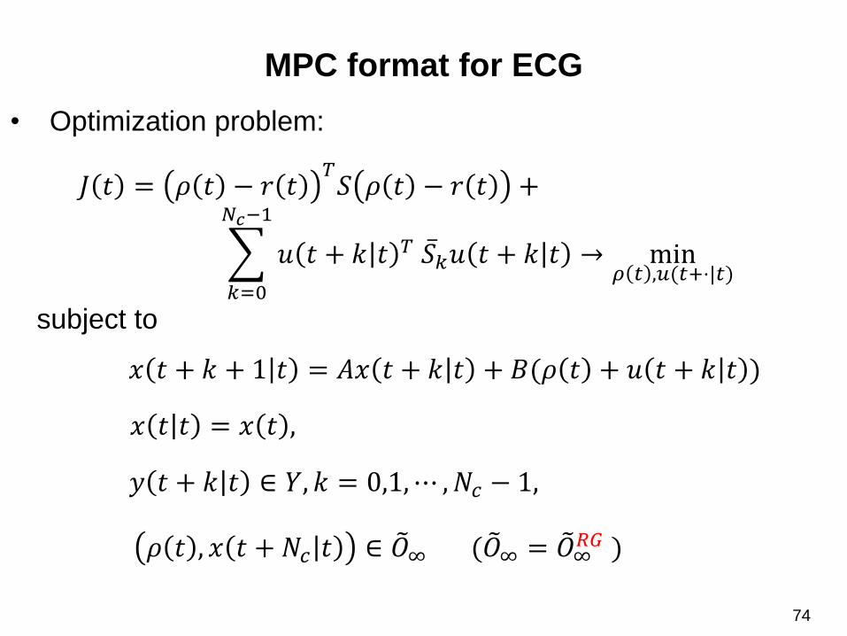
MPC format for ECG
• Optimization problem:
𝐽 𝑡 = 𝜌 𝑡 − 𝑟 𝑡𝑇𝑆 𝜌 𝑡 − 𝑟 𝑡 +
𝑘=0
𝑁𝑐−1
𝑢 𝑡 + 𝑘 𝑡 𝑇 ҧ𝑆𝑘𝑢 𝑡 + 𝑘 𝑡 → min𝜌 𝑡 ,𝑢(𝑡+⋅|𝑡)
subject to
𝑥 𝑡 + 𝑘 + 1 𝑡 = 𝐴𝑥 𝑡 + 𝑘 𝑡 + 𝐵(𝜌 𝑡 + 𝑢 𝑡 + 𝑘 𝑡 )
𝑥 𝑡 𝑡 = 𝑥 𝑡 ,
𝑦 𝑡 + 𝑘 𝑡 ∈ 𝑌, 𝑘 = 0,1,⋯ ,𝑁𝑐 − 1,
𝜌 𝑡 , 𝑥 𝑡 + 𝑁𝑐 𝑡 ∈ ෨𝑂∞ ( ෨𝑂∞ = ෨𝑂∞𝑅𝐺 )
74

MPC format for ECG
• Condition that must hold: ҧ𝑆𝑘 ≥ ҧ𝑆𝑘−1 ≥ ⋯ ≥ ҧ𝑆0> 0
• ECG theory provides recursive feasibility and finite-time
convergence results for this special class of MPC
controllers, i.e., it guarantees that
𝜌 𝑡 = 𝑟 𝑡 , 𝑢 𝑡 + 𝑘 𝑡 = 0, 𝑘 = 0,⋯ ,𝑁𝑐 − 1
for all 𝑡 ≥ 𝑡𝑠 and for constant, strictly constraint
admissible, 𝑟 𝑡 = 𝑟𝑠.
75

Extended Command Governor (f16aircraft_ecg.m)
% --------- Construct appended system for ECG -----
nh = 5;
[sys_app, sys_full] = ecg_appdyn(nh, ss(A,B,C,D,dT),'laguerre', 0.4);
Abar = sys_app.A;
Cbar = sys_app.C;
nb = size(Abar, 1);
Secg = dlyap(Abar,0.1*eye(nb)); % weight matrix on xbar
…
Recg = diag([1,1]); % weighting matrix on rho
…
for i = 1:t_sim,
...
[v(:,i+1),p(:,i+1),rho(:,i+1)] = gov_ecg(Recg, Secg, Hx, Hp, Hr, h,x_gov(:,i+1),
r(:,i+1), sys_app.c, p(:,i), rho(:,i));
…
end76
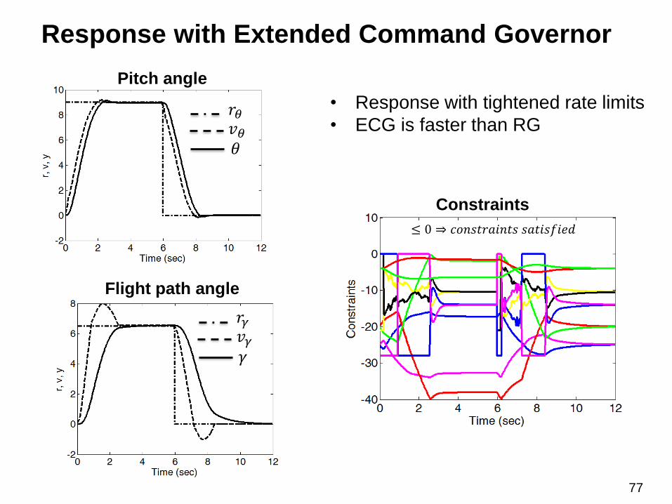
Response with Extended Command Governor
Pitch angle
Flight path angle
𝑟𝜃𝑣𝜃𝜃
𝑟𝛾𝑣𝛾𝛾
• Response with tightened rate limits
• ECG is faster than RG
≤ 0 ⇒ 𝑐𝑜𝑛𝑠𝑡𝑟𝑎𝑖𝑛𝑡𝑠 𝑠𝑎𝑡𝑖𝑠𝑓𝑖𝑒𝑑
Constraints
77

The Set ෩𝑶∞ (with disturbances, 𝑾 is polyhedral)
𝐻𝜌,𝑡 𝜌 + 𝐻 ҧ𝑥,𝑡 ҧ𝑥 0 +𝐻𝑥,𝑡 𝑥 0 ≤ 𝜆𝑡
𝐻∞𝜌 ≤ 𝜆∞
𝑌𝑡 = 𝑦: Λ𝑦 ≤ 𝜆𝑡 = 𝑌 ∼ 𝐷𝑤𝑊 ∼ 𝐶𝐵𝑤𝑊 ∼ ⋯ ∼ 𝐶𝐴𝑡−1𝐵𝑤𝑊
𝜆𝑡 = 𝜆𝑡−1 −maxሼ𝑊 𝑖
Λ𝐶𝐴𝑡−1𝐵𝑤𝑊𝑖 }, 𝑡 > 1
𝑌∞ = 𝑦: Λ𝑦 ≤ 𝜆∞ , 0 < 𝜆∞ < inf𝑡𝜆𝑡
• ෨𝑂∞ is defined by affine inequalities on 𝜌, ҧ𝑥 0 , 𝑥 0 :
𝜆0 = 𝜆 −maxሼ𝑊 𝑖
Λ𝐷𝑤𝑊𝑖 }
𝑊 = 𝑐𝑜𝑛𝑣ℎሼ𝑊(𝑖), 𝑖 = 1,⋯ , 𝑛𝑤}
(𝑡 = 0,12,⋯ )
78

Reference Governors for
Nonlinear Systems
79

Nonlinear systems with pointwise-in-time
constraints
Control objectives
• Tracking: 𝑧 𝑡 ≈ 𝑟(𝑡)• Satisfy pointwise-in-time state/control constraints: 𝑦 𝑡 ∈ 𝑌• Robustness to disturbances/uncertainties: 𝑤 𝑡 ∈ 𝑊 ∀𝑡 ≥ 0• Optimality
• obstacle avoidance
• actuator limits
• safety limits
• …
𝑦 𝑡 ∈ 𝑌 ∀𝑡 ≥ 0
80

Nonlinear systems with constraints,
disturbances, and commands
• Stationary disturbances 𝑤 𝑡 :
• Nonlinear system with constraints, disturbances and
commands
𝑥 𝑡 + 1 = 𝑓(𝑥 𝑡 , 𝑣 𝑡 , 𝑤 𝑡 )
𝑦 𝑡 ∈ 𝑌 ⇔ (𝑥 𝑡 , 𝑣 𝑡 ) ∈ 𝐶 ∀𝑡 ∈ 𝑍+
Gilbert and Kolmanovsky, Automatica (38) 2063-2073 (2002)
- set-bounded
- set-bounded and rate bounded
- parametric uncertainties
- …
12/14/2014
𝑤 ⋅ ∈ 𝕎 ⇒ 𝑤 ⋅ +𝜎 ∈ 𝕎 𝑓𝑜𝑟 𝑎𝑙𝑙 𝜎 ∈ 𝑍+
81

Functional description of safe set of
states and constant commands
• Safe set* of initial states and constant commands
ത𝑉 𝑥(0), 𝑣(0) ≤ 0 ⇒ 𝑥 𝑡 , 𝑣 0 ∈ 𝐶 ∀𝑡 ∈ 𝑍+
- ത𝑉 is continuous (can be non-smooth)
- Strong returnability:
ത𝑉 𝑥(𝑡), 𝑣(0) ≤ −𝜖 for some 𝑡 ∈ 𝑍+
𝑥 𝑡 = 𝑥 𝑡 𝑥 0 , 𝑣 𝑘 = 𝑣 0 , 𝑘 = 1,⋯ , 𝑡 − 1
• Technical assumptions
ത𝑉 𝑥(0), 𝑣(0) ≤ 0 ⇒
*Safe set is not required to be positively invariant82

Functional description of safe set of
states and constant commands
83

Scalar reference governor
subject to
• Maximize 𝛽(𝑡)
ത𝑉 𝑥(𝑡), 𝑣(𝑡) ≤ 0,
𝑣 𝑡 = 𝑣 𝑡 − 1 + 𝛽 𝑡 𝑟 𝑡 − 𝑣 𝑡 − 1 ,
• 𝛽 𝑡 = 0 if no feasible solution exists
• Accept small increments, 𝑣 𝑡 − 𝑣 𝑡 − 1 , only if ത𝑉 𝑥(𝑡), 𝑣(𝑡 − 1) ≤ −𝜖
0 ≤ 𝛽(𝑡) ≤ 1
• Solution via bisections or grid search, explicit in some cases (e.g., if ത𝑉 is quadratic)
• Solution within a known tolerance is sufficient for subsequent theoretical results to hold.
84

Reference governor: basic approach
ത𝑉 𝑥, 𝑣(𝑡) ≤ 0
ത𝑉 𝑥, 𝑣(𝑡 + 4) ≤ 0
85

Definitions
Π 𝑞 = ሼ𝑥: ത𝑉 𝑥, 𝑞 ≤ 0} is a “safe” set with 𝑣 𝑡 = 𝑞
Π𝜀 𝑞 = ሼ𝑥: ത𝑉 𝑥, 𝑞 ≤ −𝜖}
• Let 𝑆 be a compact and convex set such that for 𝑣 ∈ 𝑆technical assumptions hold
• For 𝑞 ∈ 𝑆 define:
86
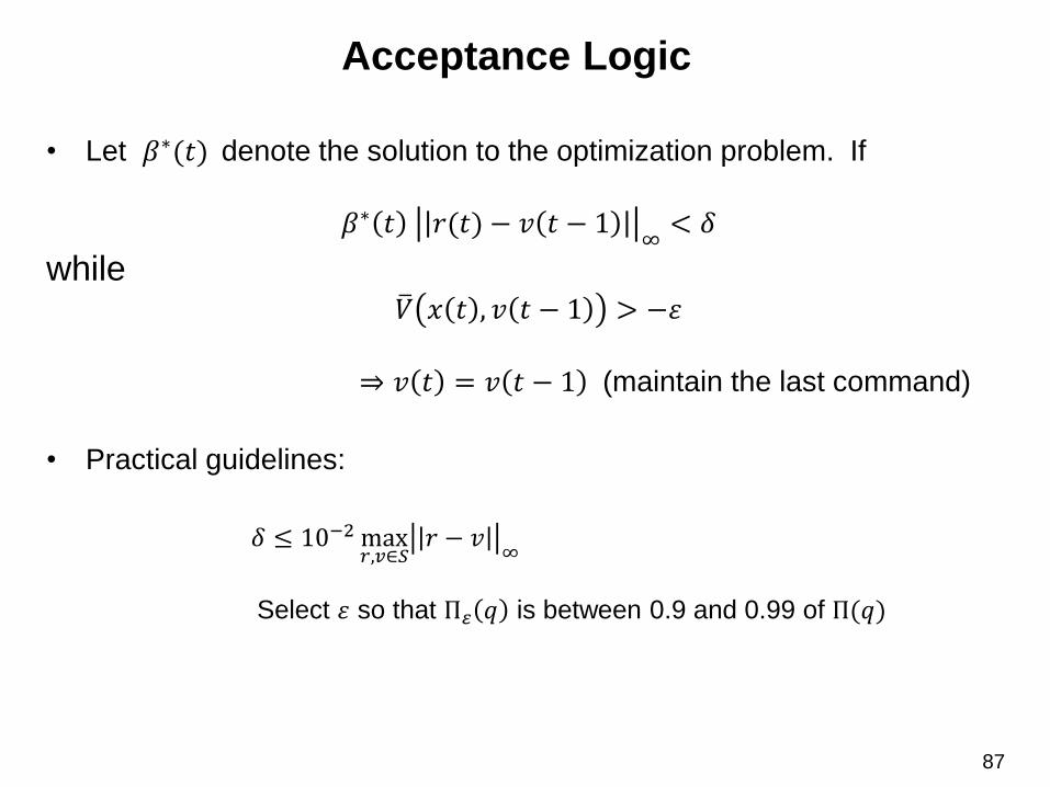
Acceptance Logic
• Let 𝛽∗(𝑡) denote the solution to the optimization problem. If
𝛽∗ 𝑡 𝑟(𝑡) − 𝑣 𝑡 − 1∞< 𝛿
whileത𝑉 𝑥 𝑡 , 𝑣 𝑡 − 1 > −휀
⇒ 𝑣 𝑡 = 𝑣 𝑡 − 1 (maintain the last command)
• Practical guidelines:
𝛿 ≤ 10−2max𝑟,𝑣∈𝑆
𝑟 − 𝑣∞
Select 휀 so that Π𝜀 𝑞 is between 0.9 and 0.99 of Π(𝑞)
87
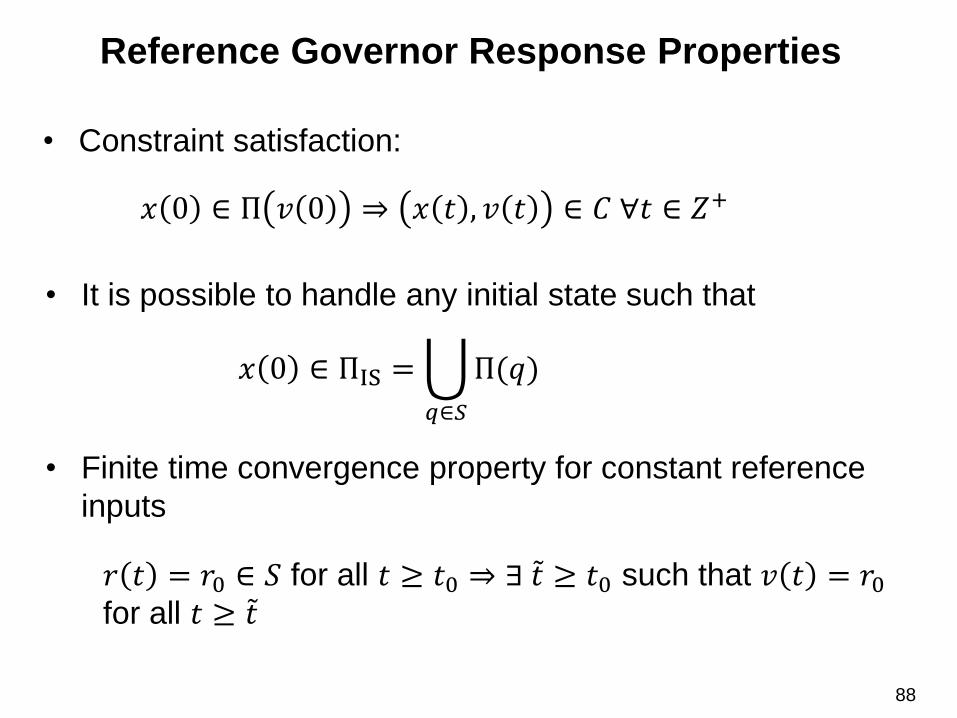
Reference Governor Response Properties
• Constraint satisfaction:
𝑥 0 ∈ Π 𝑣 0 ⇒ 𝑥 𝑡 , 𝑣 𝑡 ∈ 𝐶 ∀𝑡 ∈ 𝑍+
• It is possible to handle any initial state such that
𝑥 0 ∈ ΠIS =ራ
𝑞∈𝑆
Π(𝑞)
• Finite time convergence property for constant reference
inputs
𝑟 𝑡 = 𝑟0 ∈ 𝑆 for all 𝑡 ≥ 𝑡0 ⇒ ∃ ǁ𝑡 ≥ 𝑡0 such that 𝑣 𝑡 = 𝑟0for all 𝑡 ≥ ǁ𝑡
88

Reference Governor Response Properties
• Response properties for non-constant inputs:
𝑟 𝑡 − 𝑟0 ∞≤ 𝛿0 for all 𝑡 ≥ 𝑡0, 𝑟0 ∈ 𝑆, and 0 < 𝛿0 <
1
2𝛿,
Then if 𝛿 is sufficiently small ⇒ 𝑣 𝑡 − 𝑟0 ∞≤ 𝛿0 for all 𝑡
sufficiently large
• Under additional assumptions,
𝑣 𝑡 = 𝑟(𝑡) if 𝑟 𝑡 − 𝑟0 ∞≤ 𝛿0 for all 𝑡 ≥ 𝑡0, r0 ∈ 𝑆
• Can handle additional constraints
𝑣 𝑡 − 𝑣 𝑡 − 1∞≤ 𝛿𝑚𝑎𝑥
89

Constructing ഥ𝑽
• Closed-loop Lyapunov or ISS-Lyapunov functions
- Define ത𝑉 𝑥, 𝑣 = 𝑉 𝑥, 𝑣 − 𝑐 𝑣 , where 𝑉 is a Lyapunov or an ISS-
Lyapunov function of the closed-loop system
- For a given 𝑣, maximize 𝑐 𝑣 subject to sublevel set
Π 𝑣 = ሼ𝑥: ത𝑉 𝑥. 𝑣 ≤ 0} satisfying constraints
- In cases with bounded disturbances, need 𝑐 𝑣 ≥ 𝑐𝑚𝑖𝑛(𝑣) for the
sublevel set Π(𝑣) to be strongly returnable
- Simplifications occur due to positive invariance of sublevel sets
90
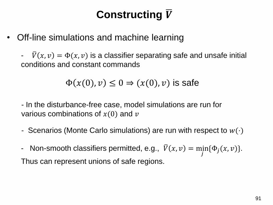
Constructing ഥ𝑽
• Off-line simulations and machine learning
- ത𝑉 𝑥, 𝑣 = Φ(𝑥, 𝑣) is a classifier separating safe and unsafe initial
conditions and constant commands
- Scenarios (Monte Carlo simulations) are run with respect to 𝑤(⋅)
- Non-smooth classifiers permitted, e.g., ത𝑉 𝑥, 𝑣 = min𝑗ሼΦ𝑗(𝑥, 𝑣)}.
Thus can represent unions of safe regions.
Φ 𝑥(0), 𝑣 ≤ 0 ⇒ (𝑥(0), 𝑣) is safe
- In the disturbance-free case, model simulations are run for
various combinations of 𝑥(0) and 𝑣
91

Constructing ഥ𝑽
𝑧 =𝑥𝑣
Φ𝑗 𝑧 = maxሼ𝜂𝑖𝑗𝑇 𝑧 − 𝑐𝑗 , 𝑖 ∈ 𝐼}
ത𝑉 𝑥, 𝑣 = ത𝑉 𝑧 = min𝑗
Φ𝑗(𝑧)
Example: Cover safe initial
conditions and commands
by a union of hyper-
rectangles
92

ഥ𝑽 implicitly defined through on-line prediction
• Constraints:
𝐶 = ሼ 𝑥, 𝑣 : ℎ𝑖 𝑥, 𝑣 ≤ 0, 𝑖 = 1,⋯ , 𝑟}
ത𝑉 𝑥, 𝑣 = 𝑚𝑎𝑥ሼℎ𝑖(𝜙 𝑡, 𝑥, 𝑣, 𝑤 ⋅ , 𝑣), 𝑖 = 1,⋯ , 𝑟, 𝑡 = 0,⋯ , 𝑡0, 𝑤 ⋅ ∈ 𝑊}
where 𝑡0 is sufficiently large so that
ℎ𝑖 𝜙 𝑡, 𝑥, 𝑣, 𝑤 ⋅ , 𝑣 ≤ −𝜖, 𝑖 = 1,⋯ , 𝑟, 𝑤 ⋅ ∈ 𝑊 and 𝑡 ≥ 𝑡0
𝜙 = “solution”
Bemporad, IEEE TAC AC-43(4) 451-461 (1998); Gilbert and K, Automatica, 38, 2063-2073, 2002
• On-line prediction of maximum constraint violation
93

ഥ𝑽 implicitly defined through on-line prediction
Sun and K., IEEE TCST 13 (6), pp. 991-919, 2005
• Simplifications in parametric uncertainty/robust reference
governor case
𝜙 𝑡, 𝑥, 𝑣, 𝑤 ≈ 𝜙 𝑡, 𝑥, 𝑣, 𝑤0 +𝜕𝜙
𝜕𝑤ቚ𝑡,𝑥,𝑣,𝑤0
(𝑤 − 𝑤0)
𝜕𝜙
𝜕𝑤|𝑡,𝑥,𝑣,𝑤0
= solution of sensitivity ODEs
94

Control of EAMSD
• Position and current constraints
Miller, K, Gilbert, Washabaugh, IEEE Control Systems Magazine,2000
𝑑𝑥1𝑑𝑡
= 𝑥2
𝑑𝑥2𝑑𝑡
=𝑘
𝑚𝑥1 −
𝑐
𝑚𝑥2 +
𝛼
𝑚
𝑢
𝑑0 − 𝑥1𝛾 , 𝑢 = 𝑖𝛽
𝑢 =1
𝛼(𝑑0 − 𝑥1 )
𝛾 𝑘𝑣 − 𝑐𝑑𝑥2
𝑑0
𝑥𝑒(𝑣)
ത𝑉 𝑥, 𝑣 =𝑘
2𝑥1 − 𝑣 2 +
𝑚
2𝑥22 − 𝑐 𝑣
Position constraint
𝑥1
𝑥2
Current constraint
ത𝑉 𝑥, 𝑣 ≤ 0
95

Control of EAMSD
Without RG
Experimental Results
With RG
• Position and current constraints
𝑑0
Position response
96

17:00-17:20, Paper FrC15.4 Add to My Program
Constrained Spacecraft Attitude Control on SO(3) Using
Reference Governors and Nonlinear Model Predictive Control
Kalabic, Uros V. Univ. of Michigan
Gupta, Rohit Univ. of Michigan
Di Cairano, Stefano Mitsubishi Electric Res. Lab.
Bloch, Anthony M. Univ. of Michigan
Kolmanovsky, Ilya V. The Univ. of Michigan
16:20-16:40, Paper WeC06.2 Add to My Program
Constraint Enforcement of Piston Motion in a Free-Piston Engine
Zaseck, Kevin Univ. of Michigan
Brusstar, Matthew The United States Environmental Protection
Agency
Kolmanovsky, Ilya V. The Univ. of Michigan
Nonlinear reference governor
applications at 2014 ACC
97

Reference Governor for Linear
Systems with Nonlinear
Constraints
98

Linear systems with nonlinear constraints
𝑥 𝑡 + 1 = 𝐴𝑥 𝑡 + 𝐵𝑣 𝑡
𝑦 𝑡 ∈ 𝑌 𝑓𝑜𝑟 𝑎𝑙𝑙 𝑡 ∈ 𝑍+
y 𝑡 = 𝐶𝑥 𝑡 + 𝐷𝑣 𝑡
𝑌 = 𝑦: ℎ𝑖 𝑦 ≤ 0, 𝑖 = 1,⋯ , 𝑟
• Linear system model:
• Treat nonlinear constraints (without polyhedral approximations):
Kalabic et. al., Proc. of 2011 CDC, pp. 2680-2686 99

Comments
• Motivation: Handling constraints for Feedback Linearizable systems
• Theory in Gilbert, K., and Tan (1994,1995) and Gilbert and K. (2002) is
applicable to the case of linear systems and nonlinear constraints
• We discuss computations, heuristics and examples
100

Scalar Reference Governor
𝛽 𝑡 ∈ 0,1 ,
𝑦 𝑡 + 𝑘|𝑡 ∈ 𝑌, 𝑘 = 0,⋯ 𝑡∗
𝛽 𝑡 → 𝑚𝑎𝑥
𝑣 𝑡 = 𝑣 𝑡 − 1 + 𝛽 𝑡 𝑟 𝑡 − 𝑣 𝑡 − 1
• Optimization problem:
1We use the approach of Bemporad (1998) with implicitly defined constraints
2Here 𝑡∗ is a finite determination index or an upper bound on it. We assume it
to be known in all the subsequent developments.
101

Linear model based prediction
𝑦 𝑡 + 𝑘|𝑡 = Γ 𝑘 𝑥 𝑡 + 𝐻 𝑘 𝑣 𝑡 − 1 + 𝛽 𝑡 𝐻 𝑘 (𝑟 𝑡 − 𝑣 𝑡 − 1 )
Γ 𝑘 = 𝐶𝐴𝑘 ,
𝐻 𝑘 = 𝐶 − Γ 𝑘 (𝐼 − 𝐴)−1𝐵 + 𝐷
• Predicted output is an affine function of 𝛽(𝑡)
• Predicted response to a constant command
𝑣 𝑡 + 𝑘|𝑡 ≡ 𝑣 𝑡 = 𝑣 𝑡 − 1 + 𝛽(𝑡)(𝑟 𝑡 − 𝑣 𝑡 )
102

Convex nonlinear constraints
If 𝛽 0 = 0 is feasible, then an admissible interval for the values of 𝛽 𝑡 is of
the form
𝐾 𝑡 = 0, 𝛽𝑚𝑎𝑥 𝑡 , 1 ≥ 𝛽𝑚𝑎𝑥 𝑡 ≥0
and the reference governor sets 𝛽 𝑡 =𝛽𝑚𝑎𝑥 𝑡 . The constraints are satisfied
for all 𝑡 ≥ 0.
• Suppose that
𝑌 = 𝑦: ℎ𝑖 𝑦 ≤ 0, 𝑖 = 1,⋯ , 𝑟
ℎ𝑖 are convex functions
• Proposition
103

Algorithmic implementation
If ℎ𝑖 𝑦 𝑡 + 𝑘 𝑡 > 0 where 𝑦 𝑡 + 𝑘 𝑡 is the predicted response with
𝛽 𝑡 = 𝛼, use bisections to search for a scalar 𝛼+ that approximately
solves
ℎ𝑖 Γ 𝑘 𝑥 𝑡 + 𝐻 𝑘 𝑣 𝑡 − 1 + 𝛼+𝐻 𝑘 𝑟 𝑡 − 𝑣 𝑡 − 1 = 0
• Set 𝛼 = 1.
• For 𝑖 = 1,⋯ , 𝑟, and 𝑘 = 0,⋯ , 𝑡∗, repeat
• Update 𝛼 = 𝛼+
• Apply “constraints active last first” evaluation heuristics (see the
paper)
104

Convex Quadratic Constraints
𝑦𝑇 ෨𝑄𝑦 + ሚ𝑆𝑦 + ሚ𝐶 ≤ 0, ෨𝑄 = ෨𝑄𝑇 ≥ 0
• Suppose that the constraints are of the form
• This is a quadratic function of 𝛽(𝑡). The root finding can be performed by
solving a quadratic equation.
• Then the constraints can be re-written as
𝑥 𝑡 𝑇 𝑣 𝑡 𝑇 + 𝛽(𝑡)(𝑟 𝑡 − 𝑣(𝑡))𝑇 ത𝑄 𝑘𝑥(𝑡)
𝑣 𝑡 + 𝛽(𝑡)(𝑟 𝑡 − 𝑣(𝑡)
+ ҧ𝑆 𝑘𝑥(𝑡)
𝑣 𝑡 + 𝛽(𝑡)(𝑟 𝑡 − 𝑣(𝑡)+ ሚ𝐶 ≤ 0
105

Mixed Logical Dynamic Constraints
𝑔𝑖 𝑦 > 0 → ℎ𝑖 𝑦 ≤ 0, 𝑖 = 1,⋯𝑟,
• We consider a set of constraints of if-then type
where 𝑔𝑖 , ℎ𝑖 are convex functions
• Observations:
• The set of β 𝑡 ∈ [0,1] for which 𝑔𝑖(𝑦 𝑡 + 𝑘 𝑡 ) ≤ 0 is a
(possibly empty) sub-interval of [0,1], 𝐾𝑖(𝑘)
• The set of β 𝑡 ∈ [0,1] for which ℎ𝑖(𝑦 𝑡 + 𝑘 𝑡 ) ≤ 0 is
another (possibly empty) sub-interval of [0,1], 𝐾𝑖(𝑘)
106

Mixed Logical Dynamic Constraints
𝑔𝑖 𝑦(𝑡 + 𝑘|𝑡) > 0 → ℎ𝑖 𝑦(𝑡 + 𝑘|𝑡) ≤ 0
• Then the set of feasible 𝛽 𝑡 ∈ [0,1] for which
is also an interval 0,1 ∩ 𝐾𝑖 𝑘 ∩ 𝐾𝑖(𝑘)
• The recursive feasibility of 𝛽 𝑡 = 0 is preserved by the reference
governor, hence it follows that the feasible values of 𝛽(𝑡) satisfy
β 𝑡 ∈ 0, 𝛽𝑚𝑎𝑥 , 𝛽𝑚𝑎𝑥 ≥ 0
107

Concave Constraints
• Suppose that the constraint functions ℎ𝑖 in Y = 𝑦: ℎ𝑖 𝑦 ≤ 0 , 𝑖 =1,⋯𝑟, are concave
• Approximate the constraints by the dynamically reconfigurable affine
constraints
𝑦(𝑡 + 𝑘|𝑡) ∈ 𝑌𝑐(𝑡)
where
𝑌𝑐 𝑡 = 𝑦: ℎ𝑖 𝑦𝑖,∗ 𝑡 +𝜕ℎ𝑖𝜕𝑦
(𝑦𝑖,∗ 𝑡 )(𝑦 − 𝑦𝑖,∗ 𝑡 ) ≤ 0 ,
𝑖 = 1,⋯ 𝑟,
and 𝑌𝑐(𝑡) ⊆ 𝑌
108

Concave Constraints
If 𝑦𝑖∗ 0 , 𝑖 = 1,⋯ 𝑟 exist such that 𝛽 0 = 0 is feasible, then
𝛽 𝑡 = 0 and 𝑦𝑖∗ 𝑡 =𝑦𝑖∗ 𝑡 − 1 remain feasible for 𝑡 > 0 and
constraints are adhered to for all 𝑡>0.
• Proposition
𝑦 𝑡
ℎ(𝑦)
𝑦𝑖∗ 𝑡
𝑦
109
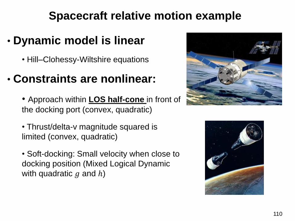
Spacecraft relative motion example
• Dynamic model is linear
• Hill–Clohessy-Wiltshire equations
• Constraints are nonlinear:
• Approach within LOS half-cone in front of
the docking port (convex, quadratic)
• Thrust/delta-v magnitude squared is
limited (convex, quadratic)
• Soft-docking: Small velocity when close to
docking position (Mixed Logical Dynamic
with quadratic 𝑔 and ℎ)
110

Spacecraft relative motion example
-1000 0 1000-300
-200
-100
0
100
200
300
Ra
dia
l p
ositio
n (
m)
Along-track position (m)-1000 0 1000
-300
-200
-100
0
100
200
300
Cro
ss-t
rack p
ositio
n (
m)
Along-track position (m)
• Reference governor is applied to
guide in-track orbital position set-point
for an unconstrained LQ controller
0 200 400 600 8000
1
2
3
4
5
time (sec)LOS cone
Dockingposition
820 830 840 8500
0.2
0.4
0.6
0.8
1
time (sec)
force (N)
Separation distance
Relative velocity
magnitude
111

Electromagnetically Actuated Mass Spring Damper
• Dynamics are feedback linearizable
• Constraints
- Current limit results in a concave nonlinear constraint
- Overshoot constraint is linear
ሶ𝑥1ሶ𝑥2
=0 1
−𝑘/𝑚 −𝑐/𝑚
𝑥1𝑥2
+0
1/𝑚𝑢
𝑢 = 𝑘𝑣 − 𝑐𝑑𝑥2
0 ≤ 𝑢 ≤𝛼 𝑖𝑚𝑎𝑥
𝛾
𝑑0 − 𝑥1𝛾
𝑥1 ≤ 0.008
force
max. current
112

Electromagnetically Actuated Mass Spring Damper
0 2 4 60
0.002
0.004
0.006
0.008
0.01
0.012
mass position x1
(m)
time (sec)
unconstrained
imax
=0.5342
imax
=0.365
0 1 2 3 4 50
0.2
0.4
0.6
0.8
current (A)
time (sec)
unconstrained
imax
=0.5342
imax
=0.365
113

Electromagnetically Actuated Mass Spring Damper
• Landing control example
• Voltage limits
• MLD constraints on soft-landing
velocity AND magnetic force
exceeding spring force
𝑑𝑧
𝑑𝑡= 𝑞
𝑑𝑞
𝑑𝑡=
1
𝑚(−𝐹𝑚𝑎𝑔 + 𝑘𝑠 𝑧𝑠 − 𝑧 − 𝑏𝑞)
𝑑𝑖
𝑑𝑡=𝑉𝑐 − 𝑟𝑖 +
2𝑘𝑎𝑖(𝑘𝑏 + 𝑧)2
𝑞
2𝑘𝑠𝑘𝑏 + 𝑧
𝐹𝑚𝑎𝑔 =𝑘𝑎
𝑘𝑏 + 𝑧 2𝑖2
114

Electromagnetically Actuated Mass Spring Damper
115