Fast and High Accuracy Numerical Methods for the Solutionof Nonlinear Klein–Gordon EquationsAkbar Mohebbia, Zohreh Asgarib, and Alimardan Shahrezaeeb

a Department of Mathematics, Faculty of Science, University of Kashan, Kashan, Iranb Department of Mathematics, Faculty of Science, Alzahra University, Tehran, Iran

Reprint requests to A. M.; E-mail: akbar mohebbi@aut.ac.ir and a mohebbi@kashanu.ac.ir

Z. Naturforsch. 66a, 735 – 744 (2011) / DOI: 10.5560/ZNA.2011-0038Received April 13, 2011 / revised July 6, 2011

In this work we propose fast and high accuracy numerical methods for the solution of the one-dimensional nonlinear Klein–Gordon (KG) equations. These methods are based on applying fourth-order time-stepping schemes in combination with discrete Fourier transform to numerically solvethe KG equations. After transforming each equation to a system of ordinary differential equations,the linear operator is not diagonal, but we can implement the methods such as for the diagonal casewhich reduces the time in the central processing unit (CPU). In addition, the conservation of energyin KG equations is investigated. Numerical results obtained from solving several problems possessingperiodic, single, and breather-soliton waves show the high efficiency and accuracy of the mentionedmethods.

Key words: Klein–Gordon Equation; Exponential Time Differencing; Integrating Factor; SpectralMethods; High Accuracy; Soliton; Conservation of Energy.

1. Introduction

The Klein–Gordon (KG) equation, that is alsoknown as Klein–Gordon–Fock equation, arises in thestudy of theoretical physics [1]. This equation isthe relativistic version of the Schrodinger equation.It represents the equation of motion of a quantumscalar or a pseudo-scalar field, which is a field whosequanta are spinless particles. Such a problem ap-pears naturally in the study of some nonlinear dy-namical problems of mathematical physics, amongthem radiation theory, general relativity of scatter-ing, and stability of kinks, vortices, and other co-herent structures. The KG equation is known as oneof the nonlinear wave equations arising in relativis-tic quantum mechanics. This equation has attractedmuch attention in studying solitons and condensedmatter physics [2], in investigating the interactionof solitons in collisionless plasma, the recurrence ofinitial states, in lattice dynamics, and in examiningthe nonlinear wave equations [1]. The KG equationplays a significant role in many scientific applicationssuch as solid state physics and nonlinear optics the-ory [3]. The nonlinear KG equation has the general

form

∂ 2u∂ t2 (x, t)−q

∂ 2u∂x2 (x, t) =

dV (u(x, t))du

,

(x, t) ∈ [a,b]× [0,T ],(1)

where dV (u(x,t))du is a nonlinear function of u chosen

as the derivative of a potential energy V (u). Equa-tion (1) occurs in a series of physical situations,as the propagation of waves in ferromagnetic ma-terials carrying rotations of the direction of magne-tization and of laser pulses in two-state media [4,7].

The nonlinear KG equations which will be exam-ined in this paper have the following forms [5, 6, 8]:

∂ 2u∂ t2 −α

2 ∂ 2u∂x2 +βu− γu2 = 0, (2)

∂ 2u∂ t2 −α

2 ∂ 2u∂x2 +αu−βu3 = 0, (3)

∂ 2u∂ t2 −α

∂ 2u∂x2 +βu− γu7 = 0, (4)

∂ 2u∂ t2 −α

2 ∂ 2u∂x2 − sin(u) = 0, (5)

c© 2011 Verlag der Zeitschrift fur Naturforschung, Tubingen · http://znaturforsch.com

736 A. Mohebbi et al. · Numerical Methods for Solving Nonlinear KG Equations

with the initial conditions

u(x,0) = ϕ1(x), x ∈ [a,b],∂u∂ t

(x,0) = ϕ2(x), x ∈ [a,b],(6)

and the periodic boundary condition

u(a, t) = u(b, t), t ∈ [0,T ]. (7)

The main property of (1) is the conservation of energy.The energy E for (1) is given by the following expres-sion [5, 9]:

E = E(t) =12

∫R

[(ut)2 +q(ux)2−2V (u)

]dx. (8)

For (2) – (5), V (u) and q are

V (u) =−β

2u2 +

γ

3u3, q = α

2,

V (u) =−α

2u2 +

β

4u4, q = α

2,

V (u) =−β

2u2 +

γ

8u8, q = α,

V (u) = 1− cos(u), q = α2,

respectively. In the literature several numericalschemes have been developed for solving KG equa-tions. Strauss and Vazquez [10] derived a three-timelevel scheme with conserved energy using standardfinite-difference approximations. Li and Vu-Quoc [11]studied the finite difference invariant structure ofa class of algorithms for the nonlinear KG equationand derived algorithms that preserve energy or linearmomentum. Jimenez and Vazquez [9] analysised fourfinite difference schemes for approximating the nonlin-ear KG equation. They observed undesirable character-istics in some of the numerical schemes, in particulara loss of spatial symmetry and the onset of instabil-ity for large values of a parameter in the initial condi-tion of the equation. In [12], an analysis of the schemesdescribed in [9] as applied to a linear problem is car-ried out, and these indicate that the instability arisesfrom the use of explicit finite difference schemes ratherthan any failure of energy conservation. This conjec-ture is further supported by an analysis of two fur-ther schemes. The KG equation is solved in [13] us-ing the variational iteration method. Guo et al. devel-oped a conservative Legendre spectral method in [14].The author of [15] obtained the approximate and/or

exact solutions of the generalized Klein–Gordon andsine-Gordon-type equations. With the aid of the sym-bolic computation system Mathematica, many exactsolutions for the KG equation with a quadratic non-linearity are constructed in [16]. Abbasbandy in [17]presented a numerical solution of nonlinear KG equa-tions with power law nonlinearities by the applica-tion of He’s variational iteration method. Dehghan andShokri in [18, 19] proposed a numerical method basedon radial bases functions. Also the boundary integralequation approach for solving the one-dimensionalsine-Gordon equation (5) is proposed in [20]. A nu-merical method based on employing the boundary in-tegral equation method and the dual reciprocity bound-ary element method (DRBEM) is suggested in [21].Some compact finite difference approaches for the so-lution of KG problems are given in [22 – 24]. A splinecollocation approach for the solution of the KG equa-tion is presented in [25]. The method of lines approachis used in [5] to transform the sine-Gordon equationinto a first-order nonlinear initial-value problem andthen replacing the matrix exponential term in a recur-rence relation by rational approximation which leadsto the second-order methods in both space and timevariables. Bratsos proposed another approach in [6] forsolving (5) which has second-order accuracy in spaceand fourth-order accuracy in the time variable. Finally,Bratsos in [4, 7] developed a predictor-corrector (PC)scheme based on the use of rational approximation ofsecond order to the matrix exponential term in a three-time level recurrence relation.

Most of the existing methods in the literature forsolving KG equations are time consuming schemesand have a low order of accuracy. In this paper wepropose some numerical schemes for solving (2) – (5)with periodic boundary conditions which are fast andaccurate. These methods are based on applying fourth-order time-stepping schemes in combination with dis-crete Fourier transform. The outline of this paper is asfollows. In Section 2, we state the spatial discretiza-tion and implementation of the methods and give anapproach to save the linear operator of the problems asdiagonal case. In Section 3, we briefly introduce theexponential integrators schemes such as the Runge–Kutta integrating factor (IFRK), the Runge–Kutta ex-ponential time differencing (ETDRK) methods, andthe Cauchy integral approach of Kassam and Tre-fethen [26] for calculating ETDRK coefficients. InSection 4, we report the numerical experiments of solv-

A. Mohebbi et al. · Numerical Methods for Solving Nonlinear KG Equations 737

ing KG equations with the applied method for severalproblems, and the conservation of energy is presented.Finally, a conclusion is drawn in Section 5.

2. Spatial Discretization

The spatial discretisation for (2) – (5) is done usinga Fourier spectral method with periodic boundary con-ditions [27, 28]. It is given a function u which is peri-odic on an appropriate spatial grid x j. From the defini-tion of discrete Fourier transform (DFT), we have [28]

uk = hN

∑j=1

eikx j u j, k =−N2

+1, ...,N2

,

in which N is the number of grid points on a periodicgrid, h is the spacing of the grid points, and k are theFourier wave numbers. The inverse DFT is

u j =1

2π

N/2

∑k=−N/2+1

eikx j uk, j = 1, . . .,N.

Let w be the nth derivative of v. For calculating w, wefirst compute v then put w = (ik)nv. We can obtain wby applying the inverse Fourier transform.

If we show the general form of (2) – (5) with utt =α2uxx + F(u, t) and put ut = v then the following sys-tem of partial differential equations (PDEs) is resulted:

ut = v

vt = α2uxx +F(u, t).

(9)

If we show U = [u v]T by applying the DFT methodto (9) and leaving the time component t, the follow-ing system of ordinary differential equations (ODEs)is obtained:

Ut = LU + N(U ), (10)

where N(U ) = [v F(u, t)]T and the linear operator Lhas the following non-diagonal form:

L2N×2N =[

0 0DN×N 0

], (11)

where DN×N is a diagonal matrix whose diagonal en-tries are −α2k2. In applying DFT in combination withexponential integrators, we need only to store D andimplement the methods as for the diagonal case. Infact, in the exponential integrators we need to calculatethe inverse and exponential of the matrix ∆tL whichhave definite structures and are stated in the followinglemmas.

Lemma 2.1 The exponential of matrix ∆tL in (11) is:

e∆tL =[

IN×N 0∆tD IN×N

],

where IN×N is the identity matrix of size N.

Proof. It is easy to check that Li = 0, i = 2,3, ...So from Taylor expansion we have e∆tL = I2N×2N+∆tL. �

We only store the vector q = [q1 q2]T, where q1 =[1, . . .,1] and q2 = −∆tα2k2, and do all computationsof the method on this vector. The next lemma is usedin ETDRK and ETDRKB methods.

Lemma 2.2 The inverse of matrix zI − ∆tL, z 6= 0,z ∈ Γ is:

(zI−∆tL)−1 =1z2 (zI +∆tL).

Proof. It is clear that zI−∆tL, z 6= 0, is invertible and(zI−∆tL)−1(zI−∆tL) = I. �

Also in this case we store vector q = [q1 q2]T, whereq1 = 1

z [1, . . .,1] and q2 = 1z2 ∆t(−α2k2), and do all com-

putations of the method on this vector.

3. Exponential Integrators

Exponential integrators are numerical schemesspecifically designed for solving differential equationswhere it is possible to discretized the original PDE intoa linear and a nonlinear part and obtain a coupled sys-tem of ODEs,

ut = Lu+N(u, t). (12)

In (12) Lu is the linear part and N(u, t) is the non-linear part. The aim of the exponential integrators isto treat the linear term exactly and allow the remain-ing part of the integration to be integrated numeri-cally using an explicit scheme. In this paper we im-plement exponential integrators of the Runge–Kuttatype. We consider the Runge–Kutta integrating fac-tor (IFRK) [26, 29, 30], the Runge–Kutta exponen-tial time differencing (ETDRK) [26, 29], and the ET-DRK method with improved accuracy by Krogstad(ETDRKB) [31]. Further, we will use the numericallystable scheme by Kassam and Trefethen [26] for cal-culating the coefficients in the ETDRK methods. Webriefly introduce these methods.

738 A. Mohebbi et al. · Numerical Methods for Solving Nonlinear KG Equations

3.1. Runge–Kutta Integrating Factor (IFRK)

The idea is to make a change of variable that allowsus to solve the linear part exactly and then use a numer-ical scheme of our choice to solve the transformed non-linear equation. Starting with our discretised PDE (12),we define

v = e−Ltu. (13)

Differentiating (13) gives

vt =−e−LtLu+ e−Ltut . (14)

If we multiply (12) by the integrating factor e−Lt , wehave

e−Ltut − e−LtLu = e−LtN(u), (15)

which gives

vt = e−LtN(eLt v). (16)

Now we can use a time-stepping method of our choiceto advance the transformed equation. We use a fourth-order Runge–Kutta formula and obtain the IFRKscheme. Regarding to (10), which is in the Fourierspace, the fourth-order formula of the IFRK methodto solve (12) is as follows [26, 29, 30]:

A = ∆tR(F(N(F−1(u)))),

B = ∆tR(F(N(F−1(e∆t L/2(u+A/2))))),

C = ∆tR(F(N(F−1(e∆t L/2u+B/2)))),

D = ∆tR(F(N(F−1(e∆t Lu+ e∆t L/2C)))),

un+1 = e∆t Lun +16(e∆t LA+2e∆t L/2(B+C)+D),

(17)

where R(.), F(.), and F−1(.) show the real part, theFourier transform, and the inverse Fourier transform ofconsidered functions, respectively.

3.2. Runge–Kutta Exponential Time Differencing(ETDRK)

The idea of the ETD methods is similar to themethod of the integrating factor. We multiply bothsides of a differential equation by some integrating fac-tor, then we make a change of variable that allows usto solve the linear part exactly. In the derivation of theETD methods, instead of making a complete change

of variable, we integrate (15) over a single time step oflength ∆t (from t = tn to t = tn+1 = tn +∆t), getting

un+1 = e∆tLun

+ e∆tL∫

∆t

0e−∆tLN(u(tn + τ), tn + τ) dτ.

(18)

The various ETD methods come from how one ap-proximates the integral in this expression. Cox andMatthews derived in [29] a set of ETD methods basedon the Runge–Kutta time stepping, which they calledETDRK methods. The fourth-order ETDRK schemeformula is as follows [29]:

un+1 = un eL∆t +αN(un, tn)+2β [N(an, tn +∆t/2)+N(bn, tn +∆t/2)]+ γN(cn, tn +∆t),

α = ∆t−2L−3[−4−∆tL+ e∆tL(4−3∆tL+(∆tL)2)],

β = ∆t−2L−3[2+∆tL+ e∆tL(−2+∆tL)],(19)

γ = ∆t−2L−3[−4−3∆tL− (∆tL)2 + e∆tL(4−∆tL)],

an = e∆tL/2un +L−1(e∆tL/2− I)N(un, tn),

bn = e∆tL/2un +L−1(e∆tL/2− I)N(an, tn +∆t/2),

cn = e∆tL/2an +L−1(e∆tL/2− I)(2N(bn, tn +∆t/2)−N(un, tn)).

It is shown in [31] that the main step of Cox–Matthewsmethod can be reproduced based on the techniquesof continuous Runge–Kutta methods. Motivated fromthe same idea, but also applied to the internal stagesof the method, a new fourth-order method is derivedin [31]. This method, which is also based on the clas-sical fourth-order Runge–Kutta method is as follows:

un+1 = e∆tLun +∆t[4φ2(∆tL)−3φ1(∆tL)+φ0(∆tL)]N(un, tn)+2∆t[φ1(∆tL)−2φ2(∆tL)]N(an, tn +∆t/2)+2∆t[φ1(∆tL)−2φ2(∆tL)]N(bn, tn +∆t/2)+∆t[4φ2(∆tL)−φ1(∆tL)]N(cn, tn +∆t/2),

where

an = e∆tL/2un +∆t/2φ0(∆tL/2)N(un, tn),

bn = e∆tL/2un +∆t/2[φ0(∆tL/2)−2φ1(∆tL/2)]·N(un, tn)+∆tφ1(∆tL/2)N(an, tn +∆t/2),

cn = e∆tLun +∆t[φ0(∆tL)−2φ1(∆tL)]N(un, tn)+2∆tφ1(∆tL)N(bn, tn +∆t).

A. Mohebbi et al. · Numerical Methods for Solving Nonlinear KG Equations 739

Also the functions φi are defined as

φ0(z) =ez−1

z, φ1(z) =

ez−1− zz2 ,

φ2(z) =ez−1− z− z2/2

z3 .

We label this fourth-order time-stepping method asETDRKB scheme to distinguish it from a standardRunge–Kutta scheme and to be consistent with the no-tation of [26, 29, 32].

Unfortunately, the ETDRK schemes suffer fromnumerical instability when the linear operator L haseigenvalues close to zero, because disastrous cancella-tion errors arise. Kassam and Trefethen in [26] havestudied these instabilities and have found that theycan be removed by evaluating a certain integral ona contour that is separated from zero. The procedureis basically to change the evaluation of the coeffi-cients, which is mathematically equivalent to the orig-inal ETDRK scheme of [29], but in [33] it has beenshown to have the effect of improving the stabilityof integration in time. Also, it easily can be imple-mented and the impact on the total computing time issmall.

The approach of [26] is to evaluate f (z) via an inte-gral over a contour in the complex plane that enclosesz and is well separated from 0 and is

f (z) =1

2π i

∫Γ

f (t)t− z

dt,

where the contour Γ must contain z in its interior andi2 =−1. This formula is the well known Cauchy inte-gral formula. It transforms our problem to one of eval-uating our function over a contour well away from theproblem area. For matrices, a similar form exists [26],i.e.

f (L) =1

2π i

∫Γ

(tI−L)−1 f (t)dt,

in which Γ is any contour that encloses the eigenval-ues of L. Contour integrals of analytic functions in thecomplex plane are easy to evaluate by means of thetrapezoid rule.

4. Numerical Experiments

To study the validity and effectiveness of thesemethods and compare the accuracy of the proposed

numerical schemes with other techniques known inthe bibliography, they are applied to various prob-lems. We performed our computations using Mat-lab 7 software on a Pentium IV, 2000 MHz CPU ma-chine with 2 Gbyte of memory. The integration in (8)was performed using the composite trapezoidal rule.In all problems we use a 512-point Fourier spec-tral discretization in x. Also we use fast Fouriertransform (FFT) routines in Matlab (i.e. fft and ifft)to calculate Fourier transform and inverse Fouriertransform.

4.1. Problem 1

Consider the partial differential equation (3),

∂ 2u∂ t2 −α

2 ∂ 2u∂x2 +αu−βu3 = 0.

We solve this PDE with two different initial conditions.

4.1.1. Periodic Waves

We consider (3) with α = 1 and β = 0.1 on the re-gion 0 < x < 1.28 and the initial conditions

ϕ1(x) = A

[1+ cos

(2πx1.28

)],

ϕ2(x) = 0.

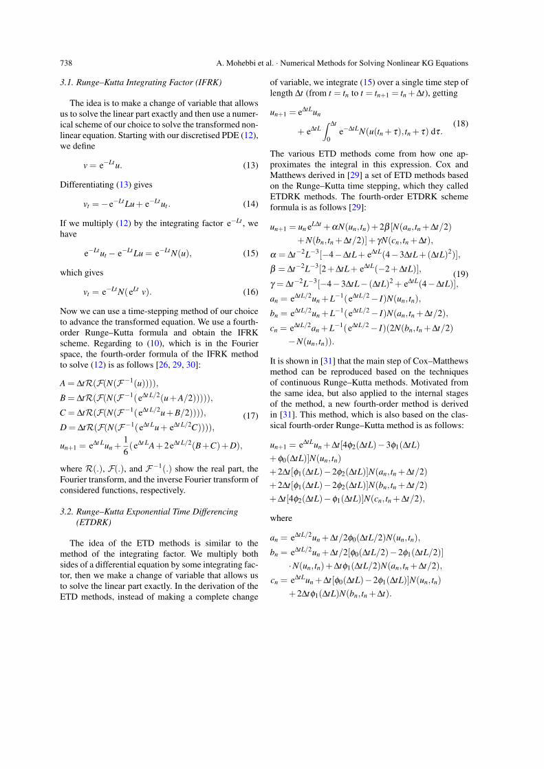
For the above problem, and due to the periodicboundary conditions, the continuous solutions remainalways symmetric with respect to the center of the spa-tial interval [4, 9]. Authors of [9] studied this prob-lem and found undesirable characteristics in some ofthe numerical schemes, in particular a loss of spatialsymmetry and the onset of instability for larger val-ues of the parameter A (amplitude) in the initial con-dition of the equation. Also, it was found that the nu-merical results given in [4] were more accurate thanthe other results given in [9, 10, 18]. In Figure 1, weshow the approximate solutions of Problem 4.1 withA = 1.5 and A = 150. As we see, the calculated ap-proximate solutions are similar to the results of [4].Also the approximate solutions obtained remain sym-metric with respect to the center of the spatial inter-val, and the solution remained bounded for amplitudeA = 150 when t ∈ [0,36]. Table 1 gives the energyE(t) at various time levels that show that the energyis conserved.

740 A. Mohebbi et al. · Numerical Methods for Solving Nonlinear KG Equations

Fig. 1 (colour online). Approximate solutions of the periodic wave problem with A = 1.5 at T = 0, 200, 1000 (left panel) andwith A = 150 at T = 0, 0.1, 36 (right panel).

Table 1. Errors of calculated energy for periodic wave withthe IFRK method when t ∈ [0, 1000] and A = 1.5, ∆t =0.001, N = 250, E(0) = 26.59641398628989.

Time (t) t = 1 t = 100 t = 500 t = 1000|E(t)−E(0)| 1.8×10−10 9.8×10−10 4.6×10−9 8.9×10−9

4.1.2. Single Soliton

We consider the partial differential equation (3) withthe following exact solution:

u(x, t)=

√2α

βsech (λ (x− ct)), −10≤ x≤ 10,

where λ =√

α

α2−c2 , α , β , α2 − c2 > 0. The initial

conditions can be obtained from the exact solution.The exact solution represents a soliton which travelswith velocity c and whose amplitude is governed bythe real parameter

√2α

β. This problem is given in [4].

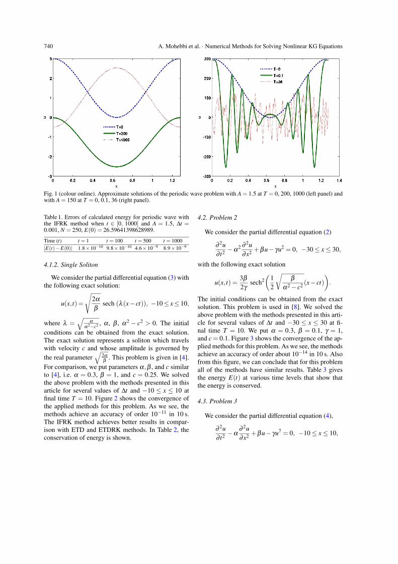
For comparison, we put parameters α,β , and c similarto [4], i.e. α = 0.3, β = 1, and c = 0.25. We solvedthe above problem with the methods presented in thisarticle for several values of ∆t and −10 ≤ x ≤ 10 atfinal time T = 10. Figure 2 shows the convergence ofthe applied methods for this problem. As we see, themethods achieve an accuracy of order 10−11 in 10 s.The IFRK method achieves better results in compar-ison with ETD and ETDRK methods. In Table 2, theconservation of energy is shown.

4.2. Problem 2

We consider the partial differential equation (2)

∂ 2u∂ t2 −α

2 ∂ 2u∂x2 +βu− γu2 = 0, −30≤ x≤ 30,

with the following exact solution

u(x, t) =3β

2γsech2

(12

√β

α2− c2 (x− ct))

.

The initial conditions can be obtained from the exactsolution. This problem is used in [8]. We solved theabove problem with the methods presented in this arti-cle for several values of ∆t and −30 ≤ x ≤ 30 at fi-nal time T = 10. We put α = 0.3, β = 0.1, γ = 1,and c = 0.1. Figure 3 shows the convergence of the ap-plied methods for this problem. As we see, the methodsachieve an accuracy of order about 10−14 in 10 s. Alsofrom this figure, we can conclude that for this problemall of the methods have similar results. Table 3 givesthe energy E(t) at various time levels that show thatthe energy is conserved.

4.3. Problem 3

We consider the partial differential equation (4),

∂ 2u∂ t2 −α

∂ 2u∂x2 +βu− γu7 = 0, −10≤ x≤ 10,

A. Mohebbi et al. · Numerical Methods for Solving Nonlinear KG Equations 741

Fig. 2 (colour online). Convergence of applied methods for single soliton problem for−10≤ x≤ 10 at final time T = 10. Themethods achieve an accuracy of order about 10−11 in 10 s.

Fig. 3 (colour online). Convergence of applied methods for Problem 2 for −30 ≤ x ≤ 30 at final time T = 10. The methodsachieve an accuracy of order about 10−14 in 10 s.

Table 2. Errors of calculated energy for single soliton withthe IFRK method when t ∈ [0, 20] and ∆t = 0.01, N = 250,E(0) = 0.11890408663357.

Time (t) t = 1 t = 5 t = 10 t = 20|E(t)−E(0)| 3.5×10−12 1.3×10−11 2.6×10−11 5.2×10−11

Table 3. Errors of calculated energy for Problem 2 with theIFRK method when t ∈ [0, 20] and ∆t = 0.01, N = 250,E(0) = 0.00314710595919.

Time (t) t = 1 t = 5 t = 10 t = 20|E(t)−E(0)| 1.2×10−16 3.1×10−16 9.2×10−16 3.0×10−14

742 A. Mohebbi et al. · Numerical Methods for Solving Nonlinear KG Equations

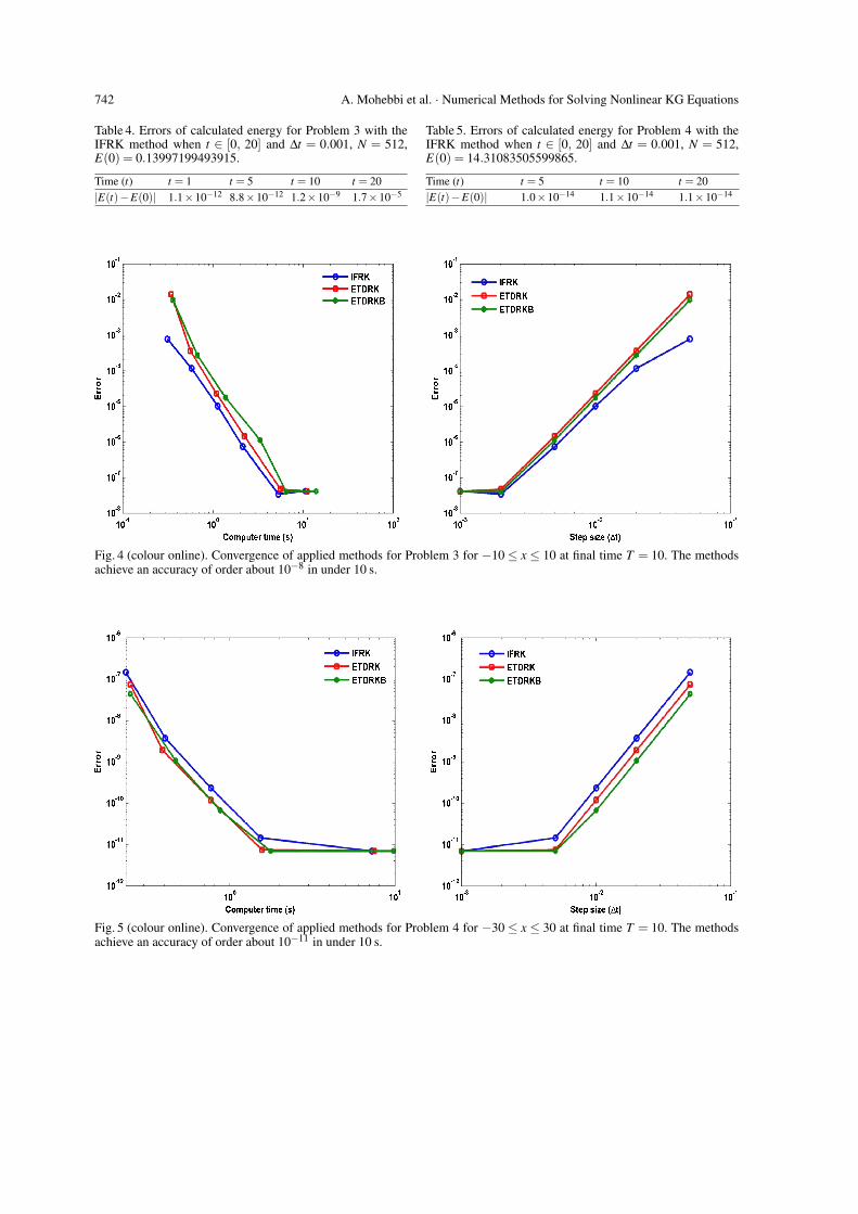
Table 4. Errors of calculated energy for Problem 3 with theIFRK method when t ∈ [0, 20] and ∆t = 0.001, N = 512,E(0) = 0.13997199493915.

Time (t) t = 1 t = 5 t = 10 t = 20|E(t)−E(0)| 1.1×10−12 8.8×10−12 1.2×10−9 1.7×10−5

Fig. 4 (colour online). Convergence of applied methods for Problem 3 for −10 ≤ x ≤ 10 at final time T = 10. The methodsachieve an accuracy of order about 10−8 in under 10 s.

Fig. 5 (colour online). Convergence of applied methods for Problem 4 for −30 ≤ x ≤ 30 at final time T = 10. The methodsachieve an accuracy of order about 10−11 in under 10 s.

Table 5. Errors of calculated energy for Problem 4 with theIFRK method when t ∈ [0, 20] and ∆t = 0.001, N = 512,E(0) = 14.31083505599865.

Time (t) t = 5 t = 10 t = 20|E(t)−E(0)| 1.0×10−14 1.1×10−14 1.1×10−14

A. Mohebbi et al. · Numerical Methods for Solving Nonlinear KG Equations 743

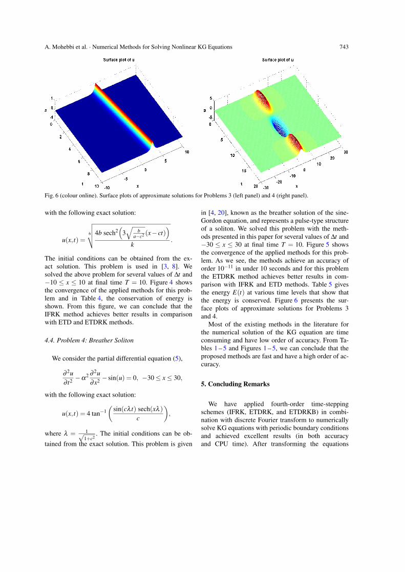
Fig. 6 (colour online). Surface plots of approximate solutions for Problems 3 (left panel) and 4 (right panel).

with the following exact solution:

u(x, t) =6

√√√√4b sech2(

3√

ba−c2 (x− ct)

)k

.

The initial conditions can be obtained from the ex-act solution. This problem is used in [3, 8]. Wesolved the above problem for several values of ∆t and−10 ≤ x ≤ 10 at final time T = 10. Figure 4 showsthe convergence of the applied methods for this prob-lem and in Table 4, the conservation of energy isshown. From this figure, we can conclude that theIFRK method achieves better results in comparisonwith ETD and ETDRK methods.

4.4. Problem 4: Breather Soliton

We consider the partial differential equation (5),

∂ 2u∂ t2 −α

2 ∂ 2u∂x2 − sin(u) = 0, −30≤ x≤ 30,

with the following exact solution:

u(x, t) = 4 tan−1(

sin(cλ t) sech(xλ )c

),

where λ = 1√1+c2

. The initial conditions can be ob-

tained from the exact solution. This problem is given

in [4, 20], known as the breather solution of the sine-Gordon equation, and represents a pulse-type structureof a soliton. We solved this problem with the meth-ods presented in this paper for several values of ∆t and−30 ≤ x ≤ 30 at final time T = 10. Figure 5 showsthe convergence of the applied methods for this prob-lem. As we see, the methods achieve an accuracy oforder 10−11 in under 10 seconds and for this problemthe ETDRK method achieves better results in com-parison with IFRK and ETD methods. Table 5 givesthe energy E(t) at various time levels that show thatthe energy is conserved. Figure 6 presents the sur-face plots of approximate solutions for Problems 3and 4.

Most of the existing methods in the literature forthe numerical solution of the KG equation are timeconsuming and have low order of accuracy. From Ta-bles 1 – 5 and Figures 1 – 5, we can conclude that theproposed methods are fast and have a high order of ac-curacy.

5. Concluding Remarks

We have applied fourth-order time-steppingschemes (IFRK, ETDRK, and ETDRKB) in combi-nation with discrete Fourier transform to numericallysolve KG equations with periodic boundary conditionsand achieved excellent results (in both accuracyand CPU time). After transforming the equations

744 A. Mohebbi et al. · Numerical Methods for Solving Nonlinear KG Equations

to a system of ordinary differential equations, thelinear operator is not diagonal, but we can imple-ment the methods such as for the diagonal caseand reduce the CPU time. For all problems theconservation of energy was investigated and thecorresponding tables were presented. It would be in-teresting to implement these methods for non-periodicboundary conditions and two-dimensional Klein–

Gordon problems which is the subject of our futurework.

Acknowledgements

The authors are very thankful to three reviewers forcarefully reading this paper and for their comments andsuggestions.

[1] R. K. Dodd, I. C. Eilbeck, J. D. Gibbon, and H. C. Mor-ris, Solitons and Nonlinear Wave Equations, Academic,London 1982.

[2] P. J. Caudrey, I. C. Eilbeck, and J. D. Gibbon, NuovoCimento 25, 497 (1975).

[3] A. M. Wazwaz, Commun. Nonlin. Sci. Numer. Simul.13, 889 (2008).

[4] A. G. Bratsos, Numer. Methods Part. Diff. Eqs. 25, 939(2009).

[5] A. G. Bratsos and E. H. Twizell, Int. J. Computer. Math.61, 271 (1996).

[6] A. G. Bratsos, Int. J. Comput. Math. 85, 1083 (2008).[7] A. G. Bratsos and L. A. Petrakis, Int. J. Comput. Math.

87, 1892 (2010).[8] A. M. Wazwaz, Chaos Solitons Fractals 28, 1005

(2006).[9] S. Jiminez and L. Vazquez, Appl. Math. Comput. 35,

61 (1990).[10] W. A. Strauss and L. Vazquez, J. Comput. Phys. 28,

271 (1978).[11] S. Li and L. Vu-Quoc, SIAM J. Numer. Anal. 32, 1839

(1995).[12] M. A. M. Lynch, Appl. Numer. Math. 31, 173 (1999).[13] F. Shakeri and M. Dehghan, Nonlin. Dyn. 51, 89

(2008).[14] B. Y. Guo, X. Li, and L. Vazquez, Math. Appl. Comput.

15, 19 (1996).[15] A. Aslanov, Z. Naturforsch. 64a, 149 (2009).[16] T. Ozis and I. Aslan, Z. Naturforsch. 64a, 15 (2009).[17] S. Abbasbandy, Int. J. Numer. Meth. Eng. 70, 876

(2007).[18] M. Dehghan and A. Shokri, J. Comput. Appl. Math.

230, 400 (2009).

[19] M. Dehghan and A. Shokri, Numer. Methods Part. Diff.Eqs. 24, 687 (2008).

[20] M. Dehghan and D. Mirzaei, Numer. Methods Part.Diff. Eqs. 24, 1405 (2008).

[21] M. Dehghan and A. Ghesmati, Comput. Phys. Com-mun. 181, 1410 (2010).

[22] M. Dehghan, A. Mohebbi, and Z. Asgari, Numer. Al-gor. 52, 523 (2009).

[23] A. Mohebbi and M. Dehghan, Math. Comput. Modell.51, 537 (2010).

[24] A. Golbabai and M. M. Arabshahi, Phys. Scr. 83,015015 (2011).

[25] S. A. Khuri and A. Sayfy, Appl. Math. Comput. 216,1047 (2010).

[26] A. K. Kassam and L. N. Trefethen, SIAM J. Sci. Com-put. 26, 1214 (2005).

[27] J. P. Boyd, Chebyshev and Fourier Spectral Methods,second edn., Dover, New York 2001.

[28] L. N. Trefethen, Spectral Methods in Matlab, SIAM,Philadelphia 2000.

[29] S. M. Cox and P. C. Matthews, J. Comput. Phys. 176,430 (2002).

[30] B. Fornberg and T. A. Driscoll, J. Comput. Phys. 155,456 (1999).

[31] S. Krogstad, J. Comput. Phys. 203, 72 (2005).[32] R. V. Craster and R. Sassi, Spectral Algorithms for

Reaction-Diffusion Equations, 2006, Technical Report,Note del Polo di Ricerca N.99, Universita di Milano,Polo di Ricerca di Crema.

[33] Q. Du and W. Zhu, BIT Numer. Math. 45, 307 (2005).