Embed Size (px)
Citation preview
BULLETIN OF THE POLISH ACADEMY OF SCIENCESTECHNICAL SCIENCES, Vol. 62, No. 4, 2014DOI: 10.2478/bpasts-2014-0078
INFORMATICS
High-accuracy numerical integration methods for fractional order
derivatives and integrals computations
D.W. BRZEZIŃSKI∗ and P. OSTALCZYK
Faculty of Electrical, Electronic, Computer and Control Engineering, Institute Of Applied Computer Science,Lodz University of Technology, 18/22 Stefanowskiego St., 90-537 Łódź, Poland
Abstract. In this paper the authors present highly accurate and remarkably efficient computational methods for fractional order derivativesand integrals applying Riemann-Liouville and Caputo formulae: the Gauss-Jacobi Quadrature with adopted weight function, the DoubleExponential Formula, applying two arbitrary precision and exact rounding mathematical libraries (GNU GMP and GNU MPFR). Examplefractional order derivatives and integrals of some elementary functions are calculated. Resulting accuracy is compared with accuracy achievedby applying widely known methods of numerical integration. Finally, presented methods are applied to solve Abel’s Integral equation (inAppendix).
Key words: accuracy of numerical calculations, fractional order derivatives and integrals, double exponential formula, gauss-jacobi quadraturewith adopted weight function, arbitrary precision, numerical integration, abel’s integral equation.
1. Introduction
There are several formulae [1–3] which can be used to com-pute integrals and derivatives of non-integer (fractional) or-ders. They include the Riemann-Liouville/Caputo formulaeand the Grunwald-Letnikov method.
In this paper the authors focus on applying the Riemann-Liouville/Caputo formulae. To investigate a problem of in-creasing numerical calculations accuracy, the authors applytwo methods never used before for such purposes: Gauss-Jacobi Quadrature and Double Exponential Transformation.Additionally application of arbitrary precision instead of dou-ble precision to further increase accuracy of two mentionedmethods is researched. The Grunwald-Letnikov formula isused for comparison purposes only. A level of accuracy ob-tained by this formula is treated as one of points of reference.
Despite the most modern computers and comprehen-sive numerical calculations knowledge, problems connect-ed with difficult kernel integrand included in Riemann-Liouville/Caputo formulae are not solved, because of the sin-gularity at the end point [3–5].
Main motivation for the following research is to solve thisdifficult computational problem. Second one is to develop ahigh accurate integration method, which can be applied ina collocation method for solving numerically fractional orderdifferential equations. The increased calculations accuracy en-ables the authors for more reliable simulations of the closeloop dynamic systems control.
Some preliminary high accuracy results proof of the de-veloped methods of integration are presented in appendix tosolve integration part of Abel’s integral equation of the 1st
kind.
2. Mathematical preliminaries
The Riemann-Liouville definition of the fractional integral oforder α > 0 is given as
RLt0I
αt f (t) =
1
Γ (α)
t∫
t0
(t − τ)α−1
f (τ) dτ ,
(α > 0) ,
(1)
where Γ is the gamma function.Riemann-Liouville Fractional Derivative is defined as
RLt0D
αt f (t)
=1
Γ (n − α)
(
d
dt
)nt
∫
t0
(t − τ)n−α−1
f (τ) dτ ,(2)
Caputo Fractional Derivative is defined as
C0D
αt f (t) =
1
Γ (n − α)
t∫
0
(t − τ)n−α−1
f (n) (τ) dτ , (3)
where α > 0, n is the smallest integer greater than or equal
to α, and the operator
(
d
dt
)n
, f (n) denote the ordinary dif-
ferential operator (of integer order).Formulae (2) and (3) are related by the formula
RLt0D
αt f (t) = C
0Dαt f (t) +
n−1∑
i=0
ti−α
Γ (i − α + 1)f (i) (0) ,
(4)For the last condition we may switch between the two (2), (3)as necessary [1–3].
∗e-mail: [email protected]
723
Brought to you by | University of Technology LódzAuthenticated
Download Date | 1/22/16 8:10 AM
D.W. Brzeziński and P. Ostalczyk
Grunwald-Letnikov formula of Fractional Order BackwardDifference/Sum is defined as the derivative of a real orderα > 0 (for the integral we use order −α < 0) of a continuousbounded function f(t)
GL∆αf (t) = limh → 0
t−t0h
∑
i=0
a(α)i f (t − hi)
hα, (5)
where
a(α)i =
1 for i = 0
a(α)i−1
(
1 −1 + α
i
)
for i = 1, 2, 3, . . .(6)
3. Numerical problem formulation and research
plan
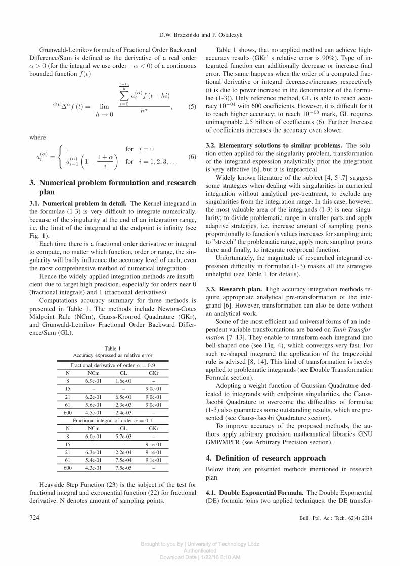
3.1. Numerical problem in detail. The Kernel integrand inthe formulae (1-3) is very difficult to integrate numerically,because of the singularity at the end of an integration range,i.e. the limit of the integrand at the endpoint is infinity (seeFig. 1).
Each time there is a fractional order derivative or integralto compute, no matter which function, order or range, the sin-gularity will badly influence the accuracy level of each, eventhe most comprehensive method of numerical integration.
Hence the widely applied integration methods are insuffi-cient due to target high precision, especially for orders near 0(fractional integrals) and 1 (fractional derivatives).
Computations accuracy summary for three methods ispresented in Table 1. The methods include Newton-CotesMidpoint Rule (NCm), Gauss-Kronrod Quadrature (GKr),and Grunwald-Letnikov Fractional Order Backward Differ-ence/Sum (GL).
Table 1Accuracy expressed as relative error
Fractional derivative of order α = 0.9
N NCm GL GKr
8 6.9e-01 1.6e-01 –
15 – – 9.0e-01
21 6.2e-01 6.5e-01 9.0e-01
61 5.6e-01 2.3e-03 9.0e-01
600 4.5e-01 2.4e-03 –
Fractional integral of order α = 0.1
N NCm GL GKr
8 6.0e-01 5.7e-03 –
15 – – 9.1e-01
21 6.3e-01 2.2e-04 9.1e-01
61 5.4e-01 7.5e-04 9.1e-01
600 4.3e-01 7.5e-05 –
Heavside Step Function (23) is the subject of the test forfractional integral and exponential function (22) for fractionalderivative. N denotes amount of sampling points.
Table 1 shows, that no applied method can achieve high-accuracy results (GKr’ s relative error is 90%). Type of in-tegrated function can additionally decrease or increase finalerror. The same happens when the order of a computed frac-tional derivative or integral decreases/increases respectively(it is due to power increase in the denominator of the formu-lae (1-3)). Only reference method, GL is able to reach accu-racy 10−04 with 600 coefficients. However, it is difficult for itto reach higher accuracy; to reach 10−08 mark, GL requiresunimaginable 2.5 billion of coefficients (6). Further Increaseof coefficients increases the accuracy even slower.
3.2. Elementary solutions to similar problems. The solu-tion often applied for the singularity problem, transformationof the integrand expression analytically prior the integrationis very effective [6], but it is impractical.
Widely known literature of the subject [4, 5 ,7] suggestssome strategies when dealing with singularities in numericalintegration without analytical pre-treatment, to exclude anysingularities from the integration range. In this case, however,the most valuable area of the integrands (1-3) is near singu-larity; to divide problematic range in smaller parts and applyadaptive strategies, i.e. increase amount of sampling pointsproportionally to function’s values increases for sampling unit;to ”stretch” the problematic range, apply more sampling pointsthere and finally, to integrate reciprocal function.
Unfortunately, the magnitude of researched integrand ex-pression difficulty in formulae (1-3) makes all the strategiesunhelpful (see Table 1 for details).
3.3. Research plan. High accuracy integration methods re-quire appropriate analytical pre-transformation of the inte-grand [6]. However, transformation can also be done withoutan analytical work.
Some of the most efficient and universal forms of an inde-pendent variable transformations are based on Tanh Transfor-
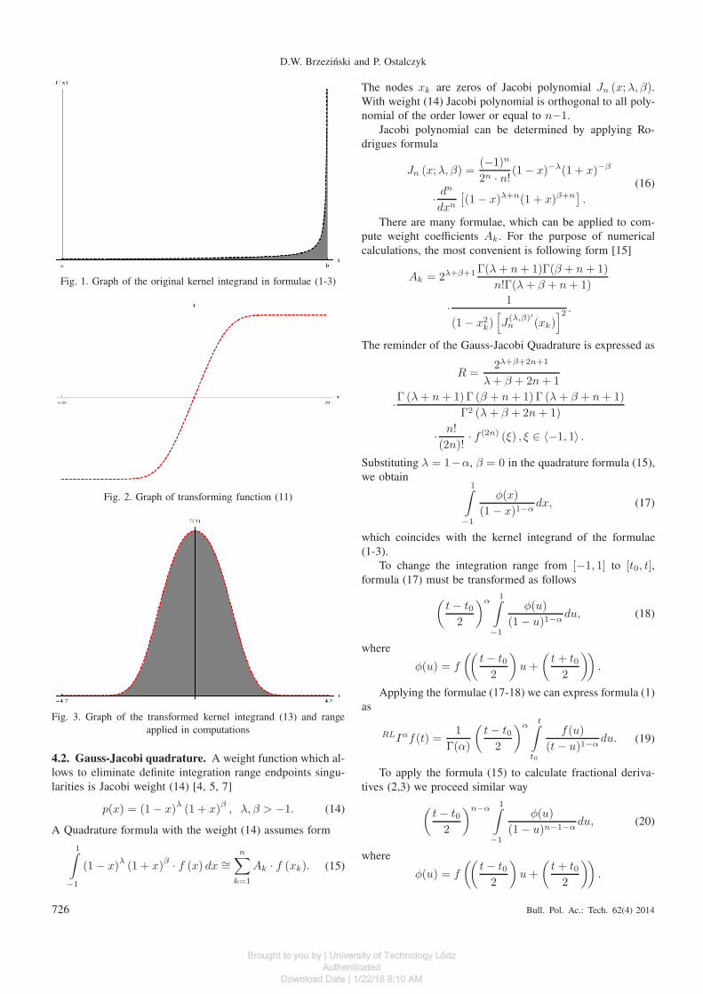
mation [7–13]. They enable to transform each integrand intobell-shaped one (see Fig. 4), which converges very fast. Forsuch re-shaped integrand the application of the trapezoidalrule is advised [8, 14]. This kind of transformation is herebyapplied to problematic integrands (see Double TransformationFormula section).
Adopting a weight function of Gaussian Quadrature ded-icated to integrands with endpoints singularities, the Gauss-Jacobi Quadrature to overcome the difficulties of formulae(1-3) also guarantees some outstanding results, which are pre-sented (see Gauss-Jacobi Quadrature section).
To improve accuracy of the proposed methods, the au-thors apply arbitrary precision mathematical libraries GNUGMP/MPFR (see Arbitrary Precision section).
4. Definition of research approach
Below there are presented methods mentioned in researchplan.
4.1. Double Exponential Formula. The Double Exponential(DE) formula joins two applied techniques: the DE transfor-
724 Bull. Pol. Ac.: Tech. 62(4) 2014
Brought to you by | University of Technology LódzAuthenticated
Download Date | 1/22/16 8:10 AM
High-accuracy numerical integration methods for fractional order derivatives and integrals computations
mation applied to the initial integrand and the trapezoidal ruleapplied to the transformed integrand.
General idea standing behind the DE transformation whichwas proposed by Schwartz [11] and become known as theTanh rule (since x = tanh(t)), is as follows:
Let’s consider the integral
I =
b∫
a
f(x)dx, (7)
where f(x) is integrable on interval (a, b). The function f(x)may have singularity x = a, x = b or at both.
First we apply the following variable transformation
x = φ(t), φ (−∞) = a, φ (∞) = b,
we obtain
I =
∞∫
−∞
f (φ(t))φ′(t)dt. (8)
Additionally, φ(t) must be equipped with special proper-ty such as φ′(t) decreases its values to 0 at, at least doubleexponential rate as t → ±∞, i.e.
|φ′(t)| → exp (−c exp (|t|)) ,
where c is some constant. After that, we apply the trapezoidalformula with an equal mesh size to the transformed integrandexpression, i.e.
I = h
∞∑
n=−∞
f (φ(nh))φ′(nh),
where nh is sampling step.Truncation of the summation process is done at some
n = −N− and n = +N+, i.e.
INh = h
N+∑
n=−N−
f (φ(nh))φ′(nh),
N = N− + N+ + 1,
(9)
where N states amount of sampling points of the function.Since φ′(nh) as well as the whole expression
f (φ(nh))φ′(nh) converges to 0 at exponential rate at large|n|, the quadrature formula (9) is called the Double Exponen-tial [7, 8, 13].
Due to truncation of the summation process (9) at somen = −N− and n = +N+ function f(x) can have singulari-ties at x = a and/or x = b as long as (7) is integrable overthe integration range.
There two kinds of errors should be taken into considera-tion when implementing the DE formula: discretization error,because we use the trapezoidal rule to approximate an inte-gral and truncation error, because we truncate infinite sum atsome N .The optimal strategy is to make both errors equal [7,8].
The subinterval widthh, which defines the evaluation step,and the number of sample points are key values in such strat-egy.
The sources [7, 8] suggest the following value of h for theDE formula
h ∼log (2π Nω/c)
N,
where c is some constant to be taken, usually 1 or π/2 andω is the distance to the nearest singularity of the integrand.
Right selection of a function with optimal properties (10-12) enables to control the level of convergence of the wholetransformed expression (9). The rate of convergence has enor-mous impact on accuracy, i.e. too rapid convergence decreasesthe accuracy [7, 8].
The authors test three different transformations and select(11) because of its optimal convergence rate for the purposeof the research, which is also suggested by the literature ofthe subject [7, 13].
The transformation expressions are as follows:
x = φ(t) = tanh tp,
φ′(t) =ptp−1
cosh2 tp, p = 1, 3, 5, . . . ,
(10)
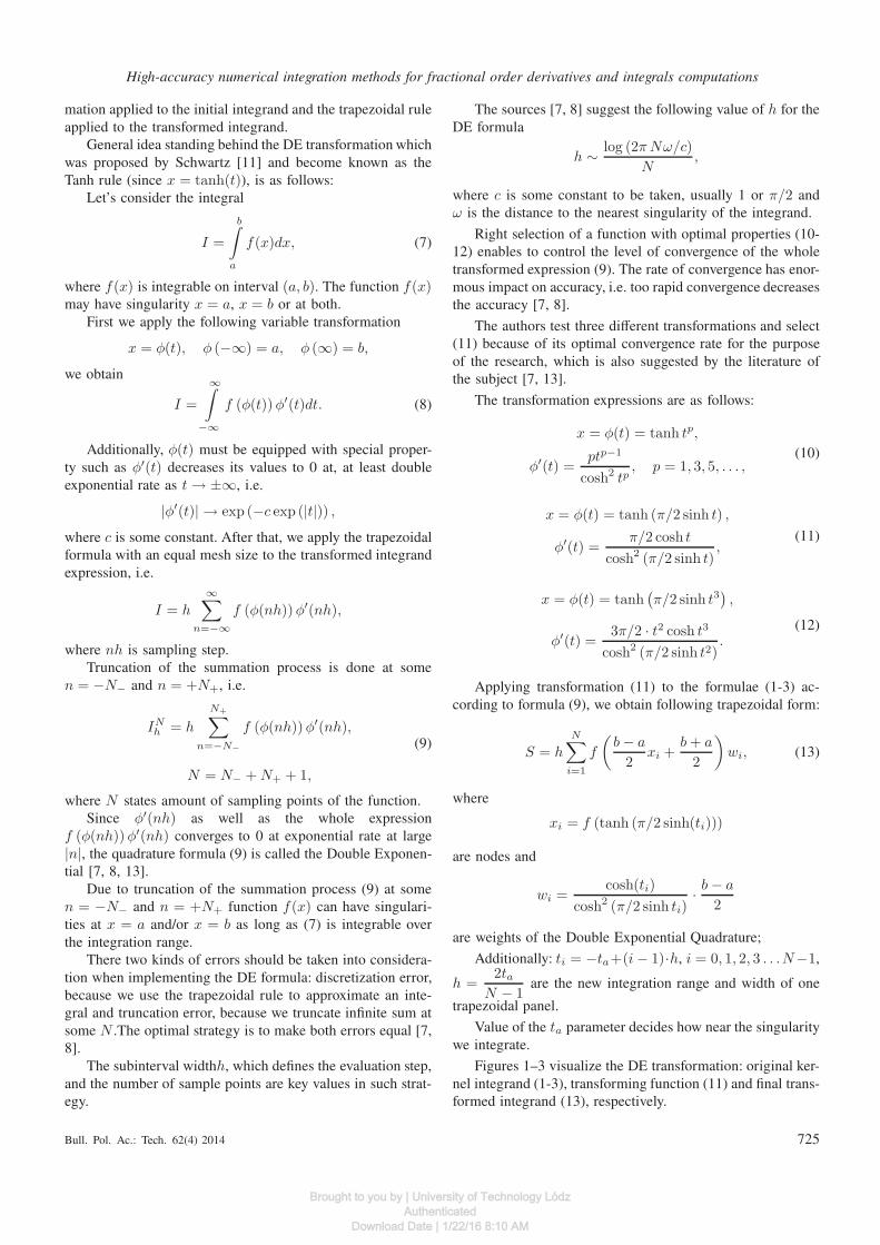
x = φ(t) = tanh (π/2 sinh t) ,
φ′(t) =π/2 cosh t
cosh2 (π/2 sinh t),
(11)
x = φ(t) = tanh(
π/2 sinh t3)
,
φ′(t) =3π/2 · t2 cosh t3
cosh2 (π/2 sinh t2).
(12)
Applying transformation (11) to the formulae (1-3) ac-cording to formula (9), we obtain following trapezoidal form:
S = hN
∑
i=1
f
(
b − a
2xi +
b + a
2
)
wi, (13)
where
xi = f (tanh (π/2 sinh(ti)))
are nodes and
wi =cosh(ti)
cosh2 (π/2 sinh ti)·b − a
2
are weights of the Double Exponential Quadrature;
Additionally: ti = −ta+(i − 1)·h, i = 0, 1, 2, 3 . . .N−1,
h =2ta
N − 1are the new integration range and width of one
trapezoidal panel.
Value of the ta parameter decides how near the singularitywe integrate.
Figures 1–3 visualize the DE transformation: original ker-nel integrand (1-3), transforming function (11) and final trans-formed integrand (13), respectively.
Bull. Pol. Ac.: Tech. 62(4) 2014 725
Brought to you by | University of Technology LódzAuthenticated
Download Date | 1/22/16 8:10 AM
D.W. Brzeziński and P. Ostalczyk
Fig. 1. Graph of the original kernel integrand in formulae (1-3)
Fig. 2. Graph of transforming function (11)
Fig. 3. Graph of the transformed kernel integrand (13) and rangeapplied in computations
4.2. Gauss-Jacobi quadrature. A weight function which al-lows to eliminate definite integration range endpoints singu-larities is Jacobi weight (14) [4, 5, 7]
p(x) = (1 − x)λ
(1 + x)β
, λ, β > −1. (14)
A Quadrature formula with the weight (14) assumes form
1∫
−1
(1 − x)λ
(1 + x)β· f (x) dx ∼=
n∑
k=1
Ak · f (xk). (15)
The nodes xk are zeros of Jacobi polynomial Jn (x; λ, β).With weight (14) Jacobi polynomial is orthogonal to all poly-nomial of the order lower or equal to n−1.
Jacobi polynomial can be determined by applying Ro-drigues formula
Jn (x; λ, β) =(−1)n
2n · n!(1 − x)−λ(1 + x)−β
·dn
dxn
[
(1 − x)λ+n(1 + x)β+n]
.
(16)
There are many formulae, which can be applied to com-pute weight coefficients Ak . For the purpose of numericalcalculations, the most convenient is following form [15]
Ak = 2λ+β+1 Γ(λ + n + 1)Γ(β + n + 1)
n!Γ(λ + β + n + 1)
·1
(1 − x2k)
[
J(λ,β)′n (xk)
]2 .
The reminder of the Gauss-Jacobi Quadrature is expressed as
R =2λ+β+2n+1
λ + β + 2n + 1
·Γ (λ + n + 1)Γ (β + n + 1)Γ (λ + β + n + 1)
Γ2 (λ + β + 2n + 1)
·n!
(2n)!· f (2n) (ξ) , ξ ∈ 〈−1, 1〉 .
Substituting λ = 1−α, β = 0 in the quadrature formula (15),we obtain
1∫
−1
φ(x)
(1 − x)1−αdx, (17)
which coincides with the kernel integrand of the formulae(1-3).
To change the integration range from [−1, 1] to [t0, t],formula (17) must be transformed as follows
(
t − t02
)α1
∫
−1
φ(u)
(1 − u)1−αdu, (18)
where
φ(u) = f
((
t − t02
)
u +
(
t + t02
))
.
Applying the formulae (17-18) we can express formula (1)as
RLIαf(t) =1
Γ(α)
(
t − t02
)αt
∫
t0
f(u)
(t − u)1−αdu. (19)
To apply the formula (15) to calculate fractional deriva-tives (2,3) we proceed similar way
(
t − t02
)n−α1
∫
−1
φ(u)
(1 − u)n−1−αdu, (20)
where
φ(u) = f
((
t − t02
)
u +
(
t + t02
))
.
726 Bull. Pol. Ac.: Tech. 62(4) 2014
Brought to you by | University of Technology LódzAuthenticated
Download Date | 1/22/16 8:10 AM
High-accuracy numerical integration methods for fractional order derivatives and integrals computations
Formula (3) assumes the following form
CDαf(t) =1
Γ(n − α)
(
t − t02
)1−α
·
t∫
t0
(t − u)n−α−1
(
d
dt
)n
f(u)du.
(21)
5. Arbitrary precision
The GNU Multiple Precision Floating-Point Reliable Library(MPFR) is an arbitrary precision package for C language andis based on GNU Multiple-Precision Library (GMP). MPFRsupports arbitrary precision floating point variables. It alsoprovides an exact rounding of all implemented operations andmathematical functions [16].
The library enables a user to set the precision of the arbi-trary precision variables precisely by specifying the numberof bits to use in the mantissa of the floating point number.Due to the design of the library, it is possible to work withany precision between 2 bits and maximum bits allowed fora computer. The ability of MPFR to set the precision exactlyto the desired precision in bits is the major difference of thislibrary in comparison with competitors. It is also the reasonfor choosing it for the following investigation.
The most common errors in numerical calculations arecaused by wrong rounding. The MPFR library supports ex-act rounding in compliance with IEEE 754-2008 standard.It implements four of the rounding modes specified by thestandard, as well as one additional not included in it:
1. Rounding to nearest, ties to even2. Round toward 03. Round toward +∞4. Round toward −∞5. Round away form 0 (not in the IEEE 754-2008 standard).
6. Numerical accuracy analysis
6.1. Integer order integration case. The purpose of the fol-lowing test is to compare the accuracy of FOD/I numericalcalculations applying two proposed methods:
• Double Exponential Quadrature (DE),• Gauss-Jacobi Quadrature (GJ),
with:
• Newton-Cotes Midpoint Rule (NCm) (modification of Rec-tagular Rule),
• Gauss-Kronord Quadrature (GKr) (modification of Gauss-Legendre Quadrature),
• Grunwald-Letnikov (GL) formula of Fractional OrderBackward Difference/Sum (4).
GKr is based on the Gauss-Legendre Rule. The G7/K15,so called Gauss-Kronrod Pair includes the nodes of the 7-point Gauss-Legendre Quadrature +8 new ones and all 15new coefficients [7]. Midpoint Rule (NCm) is a modificationof standard Rectangular Rule, which enables the application
of it to the integrands with singularities, i.e. the samplingpoints are taken in the middle of each interval.
Grunwald-Letnikov (GL) is already presented. It is theonly method dedicated to FOD/I computations.
The algorithms of the methods applied in the comparisoncan be distinguished in one main way: DE, NCm and GLuse equally spaced sampling points (coefficients in case ofGL). GJ and GKr use nth order of appropriate polynomialin approximation; sample points are zeros of the polynomi-al. Therefore it is difficult to compare the accuracy of thesemethods with the same amount of sample points. Instead, wecan ascertain how many sample points is necessary to achievetarget accuracy. In this way it is easier to find out how manyof sample points should be set for each method during themain, fractional order comparison.
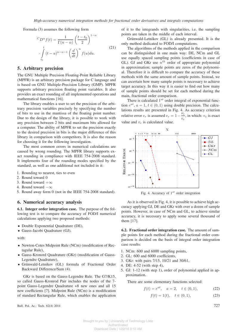
There is calculated 1st order integral of exponential func-tion eat, a = 1, t ∈ (0, 1) using double precision. The calcu-lations results are presented in Fig. 4. As accuracy criterion
relative error er is assumed er = 1−νc
ve
, in which: ve is exact
value and vc is calculated value.
Fig. 4. Accuracy of 1st order integration
As it is observed in Fig. 4, it is possible to achieve high ac-curacy applying GJ, DE and GKr with over a dozen of samplepoints. However, in case of NCm and GL, to achieve similaraccuracy, it is necessary to apply some several thousand ofthem [17].
6.2. Fractional order integration case. The amount of sam-ple points for each method during the fractional order com-parison is decided on the basis of integral order integrationcase results:
1. NCm: 600 and 6000 sampling points,2. GL: 600 and 6000 coefficients,3. GKr: with pairs 7/15, 10/21 and 30/61,4. DE: 4-52 (with step 4),5. GJ: 1-12 (with step 1), order of polynomial applied in ap-
proximation.
There are some elementary functions selected:
f(t) = eat, a = 2, t ∈ (0, 1), (22)
f(t) = 1(t), t ∈ (0, 1), (23)
Bull. Pol. Ac.: Tech. 62(4) 2014 727
Brought to you by | University of Technology LódzAuthenticated
Download Date | 1/22/16 8:10 AM
D.W. Brzeziński and P. Ostalczyk
f(t) = sin(t), t ∈ (0, 1). (24)
The integrand in formulae (1-3) is a product of two func-tions: integrated function (22-24) and kernel of Riemann-Liouville/Caputo formulae.
To illustrate the efficiency and remarkable accuracy ofthe proposed methods (GJ and DE), the authors stress in thetest the following “difficult” orders of fractional derivativesand integrals: 0.0001, 0.001, 0.01, 0.1, 0.5, 0.9, 0.99, 0.999,0.9999. In all of the tests, the same procedure is applied.
As the final part of the test, the authors compare the ac-curacy obtained applying double and arbitrary precision. Tocomplete this task two versions of the C++ code are preparedfor each proposed method of numerical integration. Arbitraryprecision code involved 100 significant digits is compared toaccuracy achieved with standard 16 significant digits availablein double precision.
7. Assumed exact values
Generally there are no analytic formulae to compute exactvalues of FOD/I for the purpose of the accuracy estimationas it is in the case of computing classical first derivative orthe integral of the 1st order.
There are however computational only formulae availablein the literature of the subject [1–3] instead. They are calcu-lated using computer and therefore, there must be taken intoconsideration some calculations error, although very small.
Assuming D−α = Iα.For function (22):
t0D−αt f(t) = tα
N∑
k=0
(at)k
Γ(k + 1 + α), (25)
t0Dαt f(t) = t−α
N∑
k=0
(at)k
Γ(k + 1 − α). (26)
For function (23)
t0D±αt f(t) =
t∓α
Γ(1 ∓ α). (27)
For function (24):
t0D−αt f(t) = tα
N∑
k=0
(at)k sin(0.5kπ)
Γ(k + 1 + α), (28)
t0Dαt f(t) =
1
tα
N∑
k=0
(at)k sin(0.5kπ)
Γ(k + 1 − α), (29)
where N is arbitrary chosen number.Additionally, key values were also confirmed comparing
the value of the classical first derivative and the integral ofthe 1st order as well as the value of the function applyingfractional order differentiation and integration operators con-catenation and fractional order differentiation and integrationof the Mittag-Leffler special function [1–3].
8. Error definition
For the purpose of the following comparison analysis, thereare calculated derivatives and integrals of selected functions(22-24) in the (0, 1) range of the fractional orders 〈0, 1〉 withstep 0.1. Additionally derivatives and integrals of “difficult”orders as for example 0.001 and 0.999 are calculated to test thedeveloped numerical integration methods abilities in the mostdifficult conditions, in which available methods of numericalintegration deliver results usually burdened with 100–200%of relative error.
The criterion of computational accuracy and the only cri-terion of the usefulness for the purpose of the research of thedeveloped methods of integration is assumed to be relativeerror er expressed as
er = 1 −νc
ve
,
where ve is a value assumed as exact obtained by calculatedapplying formulae (25-29) and vc is calculated value applyingdeveloped methods of integration.
Fractional (non-integer) order derivatives unlike classical,integer order derivatives are non local values, i.e. they arecalculated using the information from the whole range of in-tegration. It is worth explaining, that even if the selected rangefor the calculations is (0, 1), the value of the calculated deriv-ative concerns always the end of the integration range, i.e. inthis case 1 (results in Figs. 5–9, 12, 16, 17). The presentedresults in the following comparison are, however valid for anyother ranges.
Efficiency is the next part of the enclosed results present-ed as dependency of computational accuracy (expressed asrelative error) on amount of sampling points (order of poly-nomial) applied in calculations for the same method (resultsin Figs. 10–11).
Computational complexity is not the subject of the follow-ing research at the present stage of algorithms development.Additionally, due to large variation in amount of mathematicaloperations required by each of the tested integration methods,the authors decide to present at the moment only estimat-ed computational complexity in form of roughly estimatedcomputational time complexity, i.e. the computational timerequired to deliver results with desired accuracy by each ofthe methods. The charts in the this part of the comparison (inFigs. 14, 15) present the arithmetic mean value of the com-puting time calculated out of 1000 the same calculations foreach method and each function.
9. Results for double precision
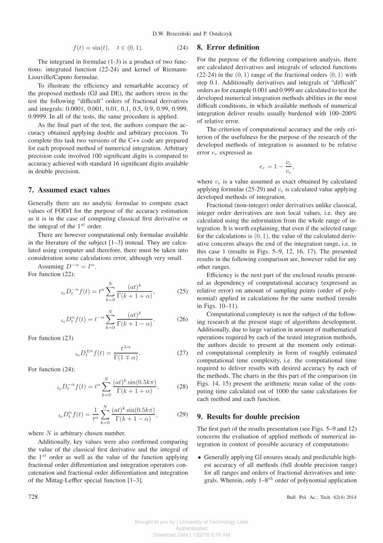
The first part of the results presentation (see Figs. 5–9 and 12)concerns the evaluation of applied methods of numerical in-tegration in context of possible accuracy of computations:
• Generally applying GJ ensures steady and predictable high-est accuracy of all methods (full double precision range)for all ranges and orders of fractional derivatives and inte-grals. Wherein, only 1–8th order of polynomial application
728 Bull. Pol. Ac.: Tech. 62(4) 2014
Brought to you by | University of Technology LódzAuthenticated
Download Date | 1/22/16 8:10 AM
High-accuracy numerical integration methods for fractional order derivatives and integrals computations
was necessary to apply, to obtain such remarkable high ac-curacy.
• Accuracy of the DE depends on order of FOD/I which isto calculate. It offers satisfactory results (half of the dou-ble precision range) only for half of tested orders. TheDE method brings higher accuracy than GJ only in highorders of fractional integrals and low orders of fractionalderivatives. Unfortunately, increasing with order power indenominator in formulae (1-3) and limitation of the trans-forming function (11) cripples the exceptional abilities ofthis, otherwise interesting method (see Fig. 13 for details).As it is observed in Fig. 12, The DE method application canincrease possible accuracy over GJ by 3-4 orders. However,with slightly more sampling points (42-56).
• GL offers steady accuracy on the level of 10−04. No sur-prise here [15].
• Other applied methods’ results are not satisfactory at all;relative error increases squarely as the order of fractionalderivative approaches 1 and fractional integral approach-es 0.
Let’s focus now on the most accurate and most efficientmethod, GJ:
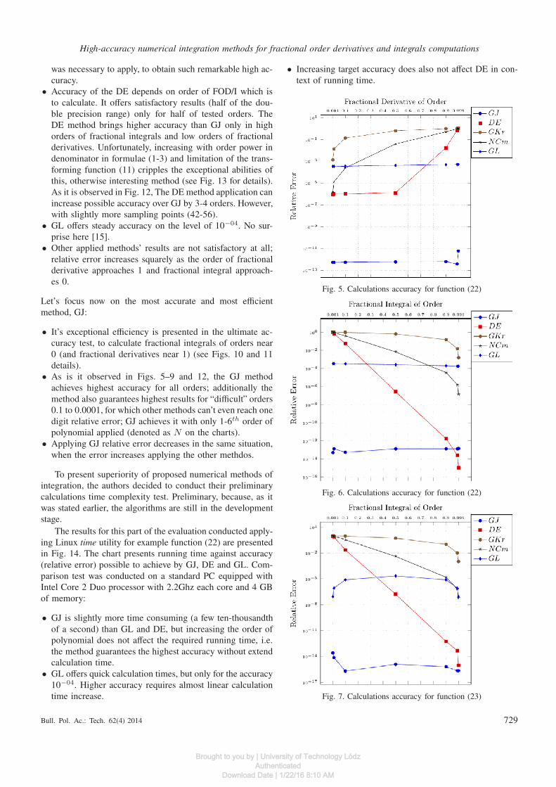
• It’s exceptional efficiency is presented in the ultimate ac-curacy test, to calculate fractional integrals of orders near0 (and fractional derivatives near 1) (see Figs. 10 and 11details).
• As is it observed in Figs. 5–9 and 12, the GJ methodachieves highest accuracy for all orders; additionally themethod also guarantees highest results for “difficult” orders0.1 to 0.0001, for which other methods can’t even reach onedigit relative error; GJ achieves it with only 1-6th order ofpolynomial applied (denoted as N on the charts).
• Applying GJ relative error decreases in the same situation,when the error increases applying the other methdos.
To present superiority of proposed numerical methods ofintegration, the authors decided to conduct their preliminarycalculations time complexity test. Preliminary, because, as itwas stated earlier, the algorithms are still in the developmentstage.
The results for this part of the evaluation conducted apply-ing Linux time utility for example function (22) are presentedin Fig. 14. The chart presents running time against accuracy(relative error) possible to achieve by GJ, DE and GL. Com-parison test was conducted on a standard PC equipped withIntel Core 2 Duo processor with 2.2Ghz each core and 4 GBof memory:
• GJ is slightly more time consuming (a few ten-thousandthof a second) than GL and DE, but increasing the order ofpolynomial does not affect the required running time, i.e.the method guarantees the highest accuracy without extendcalculation time.
• GL offers quick calculation times, but only for the accuracy10−04. Higher accuracy requires almost linear calculationtime increase.
• Increasing target accuracy does also not affect DE in con-text of running time.
Fig. 5. Calculations accuracy for function (22)
Fig. 6. Calculations accuracy for function (22)
Fig. 7. Calculations accuracy for function (23)
Bull. Pol. Ac.: Tech. 62(4) 2014 729
Brought to you by | University of Technology LódzAuthenticated
Download Date | 1/22/16 8:10 AM
D.W. Brzeziński and P. Ostalczyk
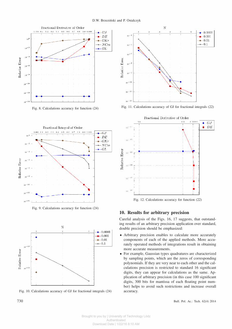
Fig. 8. Calculations accuracy for function (24)
Fig. 9. Calculations accuracy for function (24)
Fig. 10. Calculations accuracy of GJ for fractional integrals (24)
Fig. 11. Calculations accuracy of GJ for fractional integrals (22)
Fig. 12. Calculations accuracy for function (22)
10. Results for arbitrary precision
Careful analysis of the Figs. 16, 17 suggests, that outstand-ing results of an arbitrary precision application over standard,double precision should be emphasized:
• Arbitrary precision enables to calculate more accuratelycomponents of each of the applied methods. More accu-rately operated methods of integrations result in obtainingmore accurate measurements.
• For example, Gaussian types quadratures are characterizedby sampling points, which are the zeros of correspondingpolynomials. If they are very near to each other and the cal-culations precision is restricted to standard 16 significantdigits, they can appear for calculations as the same. Ap-plication of arbitrary precision (in this case 100 significantdigits, 300 bits for mantissa of each floating point num-ber) helps to avoid such restrictions and increase overallaccuracy.
730 Bull. Pol. Ac.: Tech. 62(4) 2014
Brought to you by | University of Technology LódzAuthenticated
Download Date | 1/22/16 8:10 AM
High-accuracy numerical integration methods for fractional order derivatives and integrals computations
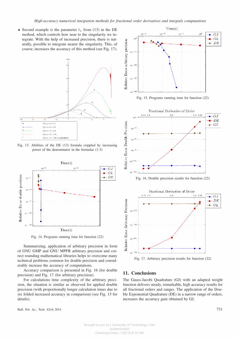
• Second example is the parameter ta from (13) in the DEmethod, which controls how near to the singularity we in-tegrate. With the help of increased precision, there is nat-urally, possible to integrate nearer the singularity. This, ofcourse, increases the accuracy of this method (see Fig. 17).
Fig. 13. Abilities of the DE (13) formula crippled by increasingpower of the denominator in the formulae (1-3)
Fig. 14. Programs running time for function (22)
Summarizing, application of arbitrary precision in formof GNU GMP and GNU MPFR arbitrary precision and cor-rect rounding mathematical libraries helps to overcome manytechnical problems common for double precision and consid-erably increase the accuracy of computations.
Accuracy comparison is presented in Fig. 16 (for doubleprecision) and Fig. 17 (for arbitrary precision).
For calculations time complexity of the arbitrary preci-sion, the situation is similar as observed for applied doubleprecision (with proportionally longer calculation times due tosix folded increased accuracy in comparison) (see Fig. 15 fordetails).
Fig. 15. Programs running time for function (22)
Fig. 16. Double precision results for function (22)
Fig. 17. Arbitrary precision results for function (22)
11. Conclusions
The Gauss-Jacobi Quadrature (GJ) with an adapted weightfunction delivers steady, remarkable, high accuracy results forall fractional orders and ranges. The application of the Dou-ble Exponential Quadrature (DE) in a narrow range of orders,increases the accuracy gain obtained by GJ.
Bull. Pol. Ac.: Tech. 62(4) 2014 731
Brought to you by | University of Technology LódzAuthenticated
Download Date | 1/22/16 8:10 AM
D.W. Brzeziński and P. Ostalczyk
The application of GNU GMP/MPFR arbitrary precisionlibraries, doubles accuracy gain of both methods.
All methods can be used as an replacement for theGrunwald-Letnikov method, which are usually applied inpractical technical applications [18–21], because they deliversteady unmatched accuracy for all orders and ranges with aremarkably low amount of sample points (6-8 instead of somehundred) and steady, short calculation times. The authors alsoplans to apply the methods to solve diffusion-wave equationwith higher accuracy, inspired by existing works [22–24].
Appendix
Abel’s integral equation. Many problems in engineering canbe solved by the Volterra integral equation of the first kind
t∫
0
k(t, s)φ(s)ds = f(t),
where f(t), k(t, s) are given functions and φ(t) is an un-known function. The function k(t, s) is the kernel of this in-tegral equation. There is a special case of this kernel, whichis the linear Abel operator
Jνφ(t) =1
Γ(ν)
t∫
0
(t − s)ν−1k(t, s)φ(s)ds,
0 ≤ t ≤ 1, 0 < ν < 1.
In the case k(t, s) = 1, the operator Jν is the classical Abeloperator.
The solution of the classical Abel integral equation
1
Γ(ν)
x∫
a
g(t)
(x − t)νdt = f(x), 0 < ν < 1, a < x < b
is given by
g(x) =1
Γ(1 − ν)
d
dx
x∫
0
(x − u)ν−1f(u)du.
There is analogy between Abel’s integral equation frac-tional order integral of a function. In fact, the fractional in-tegral of order ν of a function f(x) is just Abel operatorJνf(t).
The operator Dνf(x) =d
dxJ1−αf(x), which in fact
is (2).If f(t) = e−0.5t, 0 < t < 1, then
Jνf(x) =0 Dνt Eα,β(z),
z = az,
α = 1, β = 1, t = 1, a = −0.5.
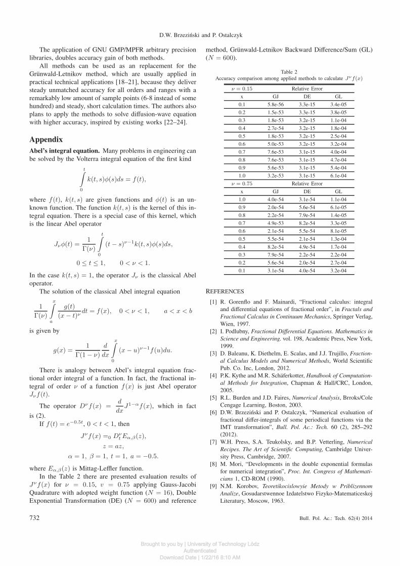
where Eα,β(z) is Mittag-Leffler function.In the Table 2 there are presented evaluation results of
Jνf(x) for ν = 0.15, v = 0.75 applying Gauss-JacobiQuadrature with adopted weight function (N = 16), DoubleExponential Transformation (DE) (N = 600) and reference
method, Grunwald-Letnikov Backward Difference/Sum (GL)(N = 600).
Table 2Accuracy comparison among applied methods to calculate Jνf(x)
ν = 0.15 Relative Error
x GJ DE GL
0.1 5.8e-56 3.3e-15 3.4e-05
0.2 1.5e-53 3.3e-15 3.8e-05
0.3 1.8e-53 3.2e-15 1.1e-04
0.4 2.7e-54 3.2e-15 1.8e-04
0.5 1.8e-53 3.2e-15 2.5e-04
0.6 5.0e-53 3.2e-15 3.2e-04
0.7 7.6e-53 3.1e-15 4.0e-04
0.8 7.6e-53 3.1e-15 4.7e-04
0.9 5.6e-53 3.1e-15 5.4e-04
1.0 3.2e-53 3.1e-15 6.1e-04
ν = 0.75 Relative Error
x GJ DE GL
1.0 4.0e-54 3.1e-54 1.1e-04
0.9 2.0e-54 5.6e-54 6.1e-05
0.8 2.2e-54 7.9e-54 1.4e-05
0.7 4.9e-53 8.2e-54 3.3e-05
0.6 2.1e-54 5.5e-54 8.1e-05
0.5 5.5e-54 2.1e-54 1.3e-04
0.4 8.2e-54 4.9e-54 1.7e-04
0.3 7.9e-54 2.2e-54 2.2e-04
0.2 5.6e-54 2.0e-54 2.7e-04
0.1 3.1e-54 4.0e-54 3.2e-04
REFERENCES
[1] R. Gorenflo and F. Mainardi, “Fractional calculus: integraland differential equations of fractional order”, in Fractals and
Fractional Calculus in Continuum Mechanics, Springer Verlag,Wien, 1997.
[2] I. Podlubny, Fractional Differential Equations. Mathematics in
Science and Engineering. vol. 198, Academic Press, New York,1999.
[3] D. Baleanu, K. Diethelm, E. Scalas, and J.J. Trujillo, Fraction-
al Calculus Models and Numerical Methods, World ScientificPub. Co. Inc, London, 2012.
[4] P.K. Kythe and M.R. Schaferkotter, Handbook of Computation-
al Methods for Integration, Chapman & Hall/CRC, London,2005.
[5] R.L. Burden and J.D. Faires, Numerical Analysis, Brroks/ColeCengage Learning, Boston, 2003.
[6] D.W. Brzeziński and P. Ostalczyk, “Numerical evaluation offractional differ-integrals of some periodical functions via theIMT transformation”, Bull. Pol. Ac.: Tech. 60 (2), 285–292(2012).
[7] W.H. Press, S.A. Teukolsky, and B.P. Vetterling, Numerical
Recipes. The Art of Scientific Computing, Cambridge Univer-sity Press, Cambridge, 2007.
[8] M. Mori, “Developments in the double exponential formulasfor numerical integration”, Proc. Int. Congress of Mathemati-
cians 1, CD-ROM (1990).[9] N.M. Korobov, Teoretikocislowyie Metody w Priblizennom
Analize, Gosudarstwennoe Izdatelstwo Fizyko-MatematiceskojLiteratury, Moscow, 1963.
732 Bull. Pol. Ac.: Tech. 62(4) 2014
Brought to you by | University of Technology LódzAuthenticated
Download Date | 1/22/16 8:10 AM
High-accuracy numerical integration methods for fractional order derivatives and integrals computations
[10] S. Haber, “The Tanh rule for numerical integration”, SIAM J.
Numer. Anal. 14, 668–685 (1999).[11] C. Schwartz, “Numerical integration of analytic functions”, J.
Computational Physics 4, 19–29 (2000).[12] F. Stenger, “Integration formulae based on the trapezoidal for-
mula”, J. Inst. Math. Appl. 12, 14 (1973).[13] H. Takahasi, Quadrature Formulas Obtained by Variable
Transformation, Springer Verlag, Berlin, 1973.[14] J. Waldvogel, “Towards a general error theory of the trape-
zoidal rule”, in Approximation and Computation 42, 267–282(2011).
[15] N. Hale and A. Townsend, “Fast and accurate computa-tion of gauss-legendre and gauss-jacobi quadrature nodes andweights”, Siam J. Sci. Comput. 35, 652–674 (2013).
[16] K.R. Ghazi, V. Lefevre, P. Theveny, and P. Zimmermann,“Why and how to use arbitrary precision”, IEEE Computer
Society 12, 5 (2010), DOI Bookmark:http://doi.ieeecomputersociety.org/10.1109/MCSE.2010.73.
[17] D.W. Brzeziński and P. Ostalczyk, “The Grunwald-Letnikovformula and its horner’s equivalent form accuracy com-parison and evaluation to fractional order PID controller”,IEEE Explorer Digital Library: IEEE Conference Publications,17
thInt. Conf. Methods and Models in Automation and Robot-
ics MMAR’12, CD-ROM (2012).
[18] M. Busłowicz and A. Ruszewski, “Necessary and suffi-cient conditions for stability of fractional discrete-time lin-ear state-space systems”, Bull. Pol. Ac.: Tech. 61 (4), 779–786(2013).
[19] T. Kaczorek, “Decoupling zeros of positive continuous-timelinear systems”, Bull. Pol. Ac.: Tech. 61 (3), 557–562 (2013).
[20] W. Mitkowski and P. Skruch, “Fractional-order models of thesupercapacitors in the form of RC ladder networks”, Bull. Pol.
Ac.: Tech. 61 (3), 581–587 (2013).[21] A. Dzielinski, G. Sarwas, and D. Sierociuk, “Comparison and
validation of integer and fractional order ultracapacitor mod-els”, Advances in Difference Equations 1, 11–23 (2011).
[22] W. Mitkowski, “Approximation of fractional diffusion-waveequation”, Acta Mechanica et Automatica 5, 65–68 (2011).
[23] A. Obrączka and W. Mitkowski, “The comparison of para-meter identification methods for fractional partial differentialequation”, Diffusion and Defect Data – Solid State Data. Part
B, Solid State Phenomena B 210, 265–270 (2014).[24] M. Błasik and M. Klimek, “Exact solution of two-term non-
linear fractional differential equation with sequential Riemann-Liouville derivatives”, Advances in the Theory and Applica-
tions of Non-integer Order Systems. Lecture Notes in Electrical
Engineering 257, 161–170 (2013).
Bull. Pol. Ac.: Tech. 62(4) 2014 733
Brought to you by | University of Technology LódzAuthenticated
Download Date | 1/22/16 8:10 AM