723

Fast-ion-beam laser-induced-fluorescence measurements ofspontaneous-emission branchingratios and oscillator strengths inSm II

S.J. Rehse, R. Li, T.J. Scholl, A. Sharikova, R. Chatelain,R.A. Holt, and S.D. Rosner

Abstract: We measured the spontaneous-emission branching ratios of 69 levels in Sm IIselectively populated via single-frequency laser excitation of a 10 keV ion beam. The levelsstudied had term energies up to 29 600 cm−1, and decay branches with spontaneous emissionin the range 250–850 nm were detected. The experimental accuracy was in the range of 10%.We used these branching ratios along with our previously determined radiative lifetimes toinfer transition probabilities and oscillator strengths for 608 transitions in the wavelengthrange 363–771 nm, which are useful for stellar abundance determinations.

PACS Nos.: 32.70.Cs, 95.30.Ky

Résumé : Nous avons mesuré les rapports de branchement d’émission spontanée de69 niveaux du Sm II peuplés de façon sélective par excitation laser à fréquence uniqued’un faisceau d’ions de 10 keV. Les niveaux excités avaient des terme d’énergies jusqu’à29 600 cm−1 et nous avons détecté des branches de désexcitation avec émission spontanéede 250 à 850 nm. La précision expérimentale était de l’ordre de 10 %. Nous avons utiliséces rapports de branchement avec des temps de vie radiatifs préalablement obtenus pourdéterminer les probabilités de transition et les forces d’oscillateur de 608 transitions dansle domaine de longueur d’onde de 363 à 771 nm qui sont utiles pour fixer les abondancesstellaires.

[Traduit par la Rédaction]

1. Introduction

A knowledge of the atomic properties of the lanthanide ions is vital to astrophysical studies ofchemically peculiar (CP) stars of the upper main sequence, metal deficient stars of the galactic halo,and the Sun [1, 2]. The lanthanides are present in CP stars in great excess in comparison with solar

Received 3 December 2005. Accepted 15 May 2006. Published on the NRC Research Press Web site athttp://cjp.nrc.ca/ on 16 September 2006.

S.J. Rehse, R. Li, T.J. Scholl, A. Sharikova, R. Chatelain, R.A. Holt, and S.D. Rosner.1 Department ofPhysics and Astronomy, University of Western Ontario, London, ON N6A 3K7, Canada.

1 Corresponding author (e-mail: rosner@uwo.ca).

Can. J. Phys. 84: 723–771 (2006) doi: 10.1139/P06-063 © 2006 NRC Canada

724 Can. J. Phys. Vol. 84, 2006

abundances; for example, in the rapidly rotating star HD101065 (Przybylski’s star), Sm II has an excessof 3.6 dex (a factor of 4 × 103) compared with its solar abundance [3]. In CP stars with measurablemagnetic-field effects, the spectral lines of the lanthanide elements are among the most enhanced [2].The galactic halo stars, which are among the oldest stars in our galaxy, have the potential to reveal thesecrets of nucleosynthesis in novae and supernovae. The lanthanides, in particular, form a contiguoussequence of atomic numbers which allow astrophysicists to study the odd–even effect resulting fromthe nuclear pairing interaction, and they present numerous examples of isotopes that may be formedby the r-process, the s-process, the p-process, or a combination. In the case of Sm, of the seven stableisotopes, 148Sm and 150Sm are produced in the stars by the s-process; 144Sm by the p-process; 154Smby the r-process; and 147Sm, 149Sm, and 152Sm by both the r- and s-processes. The study of lanthanidesin the solar spectrum is experiencing a resurgence of interest with the availability of satellite spectra inthe UV and laboratory data from new techniques. The potential contribution of two free electrons to thesolar opacity by the lanthanides, the realization that diffusion, which has had a significant fractionatingeffect on helium [4], may well have affected the heavier elements in the Sun, and increasing cautionwith regard to the accuracy of meteoritic abundances have all contributed to this renewed interest.Beyond astrophysics, the atomic properties of the lanthanides are needed in the design of commercialhigh-intensity discharge lamps [5] and in the use of spectra to probe the crystalline structure of divalentand trivalent crystal salts [2].

For a transition of known wavelength, the most important atomic property for astrophysics is itsoscillator strength f . In the case of Sm II, only a very small number of experiments have providedpublished data of modest accuracy. In the 1930s Meggers began a program of intensity measurementsat the National Bureau of Standards that led to a number of monographs listing intensities [6, 7] andoscillator strengths [8]. In the later version of these experiments, 0.1 atomic per cent of the elementunder study was incorporated in the Cu electrodes of a DC arc discharge, and the spectrum was measuredwith a rotating stepped sector to decrease the intensity of a line until it reached the limit of photographicdetectability, from which a linear measure of the line intensity could be obtained. Assumptions aboutlocal thermodynamic equilibrium, rate of entry and exit of atoms from the discharge, and negligibleself-absorption were then used by Corliss and Bozman [8] to determine absolute transition probabilities.They estimated the overall uncertainty in log gf as varying from 0.24 to 0.29 (corresponding to almosta factor of 2 in gf ) as the upper-level term energy varied from 1.5 × 104 to 5.0 × 104 cm−1. (g is themultiplicity 2J + 1 of the lower state).

A more accurate approach to determining oscillator strengths is to combine data on the branchingratios (BRs) for all transitions from a given level with a value for the spontaneous emission lifetime ofthat level. Saffman and Whaling [9] measured BRs in a hollow-cathode discharge and incorporated thebeam-foil lifetime measurements of Andersen et al. [10] to obtain oscillator strengths for transitionsfrom 9 levels of Sm II. Kurucz [11] compiled experimental oscillator strengths in a form that is availableonline [12], using the data of Saffman and Whaling, BRs from the intensity measurements of Meggerset al., together with experimental lifetime data.

Kastberg et al. [13] used optical nutation with a fast Doppler switching technique in collinear fast-ion-beam laser spectroscopy to measure the absolute transition probabilities for three lines of Sm II;the combined statistical and systematic uncertainties were on the order of 10%.

Quite recently, Xu et al. [14] performed relativistic Hartree–Fock (HFR) calculations of BRs for 47levels and combined them with their own time-resolved laser-induced-fluorescence lifetime measure-ments to calculate oscillator strengths for 162 transitions; these are available online from the DREAMdatabase [15]. The estimated uncertainties in the oscillator strength determinations were assigned oneof three values: 10%, 30%, or 50%.

Previously to the work of Xu et al. our own group measured the spontaneous-emission lifetimes of82 levels in Sm II with a fast-ion-beam laser-induced-fluorescence technique [16]. A comparison of thetwo sets of results showed agreement within experimental error (a few percent in both cases), although

© 2006 NRC Canada

Rehse et al. 725

Fig. 1. Apparatus for branching-ratio measurements. A 100 nA Sm II beam is overlapped with a collinearantiparallel single-frequency cw laser beam tuned to excite a Doppler-shifted energy level in a post-acceleration region whose potential is modulated at 5 kHz. Fluorescence from all the decay branchesis collected with arrays of optical fibers, spectrally analyzed in a Czerny–Turner monochromator, anddetected by a photomultiplier connected to a lock-in amplifier. A second identical monochromator set tothe wavelength of one of the decay branches provides a normalization signal. A data acquisition computercontrols wavelength scanning of the monochromator and records the laser-induced fluorescence intensity as afunction of wavelength, as well as the ion current, laser power, and the output of the normalization channel.A third lock-in amplifier is used to stabilize the dye-laser frequency against wavelength drift.

there was a hint of a systematic divergence for lifetimes longer than 60 ns. In the current work, we havecarried out a measurement of BRs for all levels whose lifetimes we determined in our previous study,using a new fast-ion-beam technique to be described in more detail in the following section. Using thespectrum of laser-induced fluorescence from a velocity-modulated 10 keV ion beam to measure BRs,we can identify with certainty the transitions that belong to a common upper level, and the unclutteredspectra avoid most problems due to blended lines.

© 2006 NRC Canada

726 Can. J. Phys. Vol. 84, 2006

2. Experimental method

Branching ratios for an excited atomic state are typically measured by observing the spectrum ofspontaneous emission from that state and measuring the relative intensities of the spectral lines. Previousdeterminations of branching ratios in lanthanides have utilized a hollow-cathode discharge lamp withthe element of interest contained in the cathode cavity [17]. The energy level structure in the lanthanidesis quite rich and the spontaneous emission from many levels in several ionization states is present insuch discharges, creating potential systematic errors due to spectral blending. To properly identify thebranches from specific levels of interest, comparison with previous measurements or a priori calculationsare necessary. Even still, given the sparse knowledge of the levels of Sm II, the possibility exists for themisidentification of emission lines by either omitting a branch from its correct level or attributing to alevel an emission that actually emanates from a different excited state.

The “beam-laser” method is a much more reliable spectroscopic technique that involves selectiveexcitation of a single state in a single-species ion beam followed by direct observation of the subsequentlaser-induced fluorescence [18]. All decay branches originating from this selectively populated statewith a transition wavelength within the spectral viewing range are observed and can be assigned withabsolute certainty to that excited state. Also, the signal-to-noise ratio (SNR) provided by laser excitationis excellent for typical conditions of integration times of ∼1 s or greater and ion currents of ∼50 nA orgreater.

A schematic of our experimental apparatus is shown in Fig. 1. Sm+ ions were produced in a modifiedDanfysik 911A source without an arc discharge; ionization occurred on the surface of a hot tungstenfilament. Under such conditions, we observed stable beams of ions produced in metastable levels upto ∼7100 cm−1. Ion-beam currents of ∼100 nA were typical and the actual current as detected by asecondary-electron-suppressed Faraday cup was monitored by a data acquisition computer. After accel-eration to 10 keV, the ions were focused, mass-filtered by a Wien velocity filter, and then electrostaticallydeflected to overlap a counter-propagating laser beam. Collinear geometry has three advantages, aris-ing from the Doppler effect. The spatial extent of the excitation region can be limited by utilizing theDoppler shift produced in a post-acceleration process. Modulation of the post-acceleration field andphase-sensitive fluorescence detection yields background-suppressed signals. Also, collinear geometrycreates a kinematic compression of the Doppler width, which increases signal size and makes the ex-citation process more selective [19]. Our absorption Doppler width arose primarily from the spread inthe kinetic energy of the ions, resulting in linewidths of ∼200 MHz for our beam velocities and laserfrequencies, compared to ∼2 GHz in the case of the two beams crossing at 90◦.

The single-frequency laser beam was produced by an argon-ion-pumped Coherent 699-21 dye laserrunning with Stilbene 3 dye. Stilbene 3 has a nominal tuning curve from 415–465 nm, so only Sm II levelsthat could be excited via transitions within this wavelength range were studied. The laser wavelengthwas determined to ∼1 part in 107 by a traveling Michelson interferometer with a polarization-stabilizedreference helium–neon laser [20, 21]. In the area of laser excitation and fluorescence, the laser beamwas softly focused to a 0.5 mm radius waist by a 2 m focal-length lens. Prior to entering the ion-beamvacuum chamber, the laser beam passed through multiple irises to eliminate laser light scattered fromupstream optical elements.

Ion resonance with the antiparallel propagating laser beam was confined to a small region with ahigh degree of optical access by a modification of the “Doppler-switching” technique [22]. The ionswere accelerated (and symmetrically decelerated) in regions of an electric field shaped by eight parallelconducting aperture plates separated by insulating ceramic beads (hereafter referred to as the “post-acceleration region”). A photograph of the ∼9 cm long post-acceleration region and the optical fibersused to collect laser-induced fluorescence is shown in Fig. 2. Modeling of the potential by numericalsolution of Laplace’s equation allowed us to create a highly uniform potential in the ∼3 cm centralregion. As the ions entered this region, they were accelerated by the field and brought into resonance

© 2006 NRC Canada

Rehse et al. 727

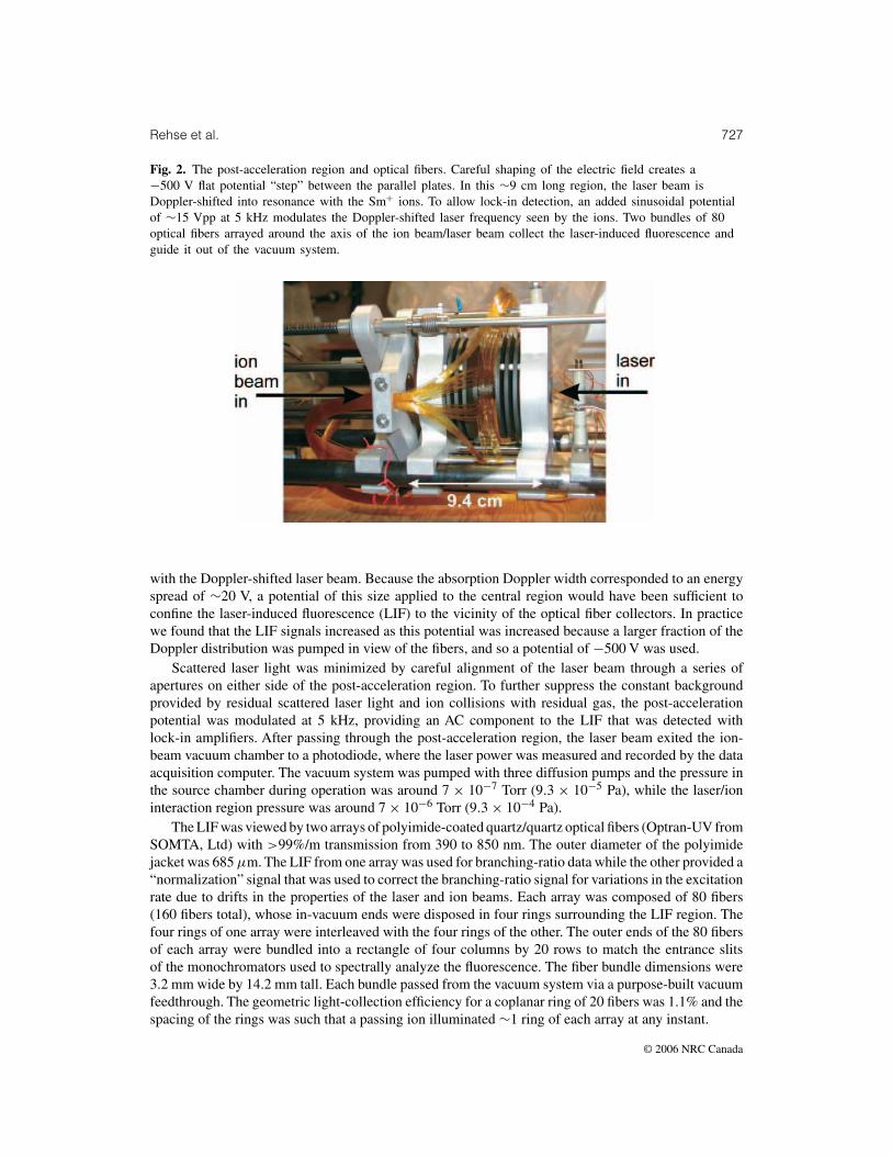
Fig. 2. The post-acceleration region and optical fibers. Careful shaping of the electric field creates a−500 V flat potential “step” between the parallel plates. In this ∼9 cm long region, the laser beam isDoppler-shifted into resonance with the Sm+ ions. To allow lock-in detection, an added sinusoidal potentialof ∼15 Vpp at 5 kHz modulates the Doppler-shifted laser frequency seen by the ions. Two bundles of 80optical fibers arrayed around the axis of the ion beam/laser beam collect the laser-induced fluorescence andguide it out of the vacuum system.

with the Doppler-shifted laser beam. Because the absorption Doppler width corresponded to an energyspread of ∼20 V, a potential of this size applied to the central region would have been sufficient toconfine the laser-induced fluorescence (LIF) to the vicinity of the optical fiber collectors. In practicewe found that the LIF signals increased as this potential was increased because a larger fraction of theDoppler distribution was pumped in view of the fibers, and so a potential of −500 V was used.

Scattered laser light was minimized by careful alignment of the laser beam through a series ofapertures on either side of the post-acceleration region. To further suppress the constant backgroundprovided by residual scattered laser light and ion collisions with residual gas, the post-accelerationpotential was modulated at 5 kHz, providing an AC component to the LIF that was detected withlock-in amplifiers. After passing through the post-acceleration region, the laser beam exited the ion-beam vacuum chamber to a photodiode, where the laser power was measured and recorded by the dataacquisition computer. The vacuum system was pumped with three diffusion pumps and the pressure inthe source chamber during operation was around 7 × 10−7 Torr (9.3 × 10−5 Pa), while the laser/ioninteraction region pressure was around 7 × 10−6 Torr (9.3 × 10−4 Pa).

The LIF was viewed by two arrays of polyimide-coated quartz/quartz optical fibers (Optran-UV fromSOMTA, Ltd) with >99%/m transmission from 390 to 850 nm. The outer diameter of the polyimidejacket was 685 µm. The LIF from one array was used for branching-ratio data while the other provided a“normalization” signal that was used to correct the branching-ratio signal for variations in the excitationrate due to drifts in the properties of the laser and ion beams. Each array was composed of 80 fibers(160 fibers total), whose in-vacuum ends were disposed in four rings surrounding the LIF region. Thefour rings of one array were interleaved with the four rings of the other. The outer ends of the 80 fibersof each array were bundled into a rectangle of four columns by 20 rows to match the entrance slitsof the monochromators used to spectrally analyze the fluorescence. The fiber bundle dimensions were3.2 mm wide by 14.2 mm tall. Each bundle passed from the vacuum system via a purpose-built vacuumfeedthrough. The geometric light-collection efficiency for a coplanar ring of 20 fibers was 1.1% and thespacing of the rings was such that a passing ion illuminated ∼1 ring of each array at any instant.

© 2006 NRC Canada

728 Can. J. Phys. Vol. 84, 2006

Fig. 3. Geometry of the 160 fluorescence-collecting fibers. The angle θ is measured with respect to thevertical linear polarization axis of the laser light (z). The laser is propagating out of the page along the axisof the rings holding the fibers (x). (a) The “magic” angle geometry. (b) The sin θ geometry.

dd

In the centre of the post-acceleration region, each individual fiber was oriented such that its opticalaxis was perpendicular to the ion/laser axis. The azimuthal positions of the fibers in each array werechosen to eliminate a specific systematic error in the evaluation of the branching ratios that could arisefrom anisotropic excitation by the linearly polarized laser beam. With the direction of the electric fieldof the vertically polarized laser defined as θ = 0, the fibers of one array were placed at or near the

“magic” angle, θmagic = cos−1(

1/√

3)

≈ 54.7◦, where the angular distribution of fluorescence from

�M = ±1 transitions has the same intensity as that for �M = 0 transitions. The fibers of the other arraywere distributed around a circle in a vertical plane with a density dN/dθ weighted as sin θ . This spacingensured that the ratio of detected fluorescence from any two branches was identical to its value in the caseof isotropic excitation or detection. These two geometric orientations are illustrated in Fig. 3. Figure 3ashows the fibers arranged in the magic angle orientation, while Fig. 3b shows the sine weighting. Thelaser was propagating in the x direction (out of the page) at the centre of the rings holding the fibers andwas vertically polarized (z) with respect to the apparatus and fibers. Branching-ratio data were collectedwith the sin θ -distributed fibers and the magic-angle bundle collected the normalization signal. A moredetailed analysis of the magic-angle and sine-weighted arrays is presented in the Appendix.

Each 80 fiber bundle terminated in a rigid coupling to the input slit of a 0.275 m, f /3.8 scanningmonochromator (Acton Research Corp.) The 20 mm high slits were normally set at their maximumwidth of 3 mm. Each monochromator had three gratings on a rotating carousel to provide completespectral coverage. The gratings had 3600, 2400, and 1200 grooves/mm with a corresponding reciprocal

© 2006 NRC Canada

Rehse et al. 729

dispersion of 1.0, 1.5, and 3.0 nm/mm, respectively. The first grating provided coverage from 250–500 nm, the second from 250–750 nm, and the third from 250–1500 nm. Since most of the Sm IIemission lines have wavelengths shorter than 500 nm, the first two gratings with superior resolutionwere used for the majority of the measurements, while the infrequent longer wavelength lines wereobserved with the third grating. In cases where closely spaced emission lines precluded the resolutionof individual lines, the entrance and exit slits of the monochromator were narrowed until the individuallines were resolved and the entire spectrum was obtained at that slit width. When measuring brancheswith wavelengths longer than 600 nm, a long-wavelength-pass filter (50% transmission point at 475 nm)was inserted prior to the PMT to avoid observation of second-order diffraction from the grating.

When it was not possible to record the entire spectrum with sufficient resolution with only onegrating, spectra obtained with multiple gratings were pieced together to provide complete spectralcoverage. When this was done, care was taken to ensure sufficient spectral overlap of the spectra. Eachgrating scan contained at least two branches, one of which was recorded by another grating; in somecases the number of branches appearing in both spectra was greater than one. The method for combiningthe data from two overlapping spectra is discussed below.

Before measurement of any branching ratios, a catalog of the potential “pump” transitions (tran-sitions used to excite the ion from a ground or metastable state to the energy level of interest) andanticipated branches was compiled from the Kurucz Atomic Line Database [11, 12]. This catalog wasused to identify all the possible branches from the level of interest that were accessible within the wave-length range of the Stilbene 3 dye-tuning curve. From these transitions, one with a large listed EinsteinA-coefficient originating from a low-lying level was chosen as the pump transition. A transition otherthan the pump transition with a large listed branching ratio was chosen as the “normalization” transition.

In Fig. 1, the “normalization” monochromator coupled with a bialkali-photocathode photomultipliertube (PMT) (Electron Tubes Ltd., 9235QB) was set to the wavelength of the normalization transition.Output from this PMT was analyzed by two lock-in amplifiers: one operating in “2f ” mode providedthe background-suppressed normalization signal, while the second, operating in “1f ” mode, provideda derivative signal for dye-laser wavelength stabilization. The normalization signal was maximized bymaking minute corrections to the ion beam steering to optimize the overlap of the laser and the ionbeam and was recorded concurrently with the branching ratio spectra on the data acquisition computer.Division of the branching ratio data by the normalization signal in software made this measurementrelatively insensitive to laser power fluctuations, ion-beam current fluctuations, and steering/pointinginstabilities in either beam. The derivative-shaped output of the 1f -mode lock-in amplifier providedan error signal that was input to the scanning control of the dye laser to lock its wavelength to thepump transition. This wavelength lock would typically hold for 15–20 min before the correction signalreached its limit and had to be manually reset to centre range.

With the laser wavelength locked to the peak of the pump-transition resonance, the “branchingratio” monochromator (Fig. 1), coupled to a thermoelectrically-cooled trialkali PMT (Electron TubesLtd., 9658R), was scanned to record the spontaneous emission spectrum from 300–850 nm and thefluorescence from the decay branches was recorded. This signal was input to a third lock-in amplifieroperating in 2f mode and its background-suppressed output was recorded on the data acquisitioncomputer, which also controlled the scanning of the monochromator grating. A typical scan would stepthe monochromator grating 1 nm per step and would dwell for 2 s per step, taking from 5 to 15 min perscan.

A typical branching ratio spectrum with excellent SNR is shown in Fig. 4. The energy level at26 540.119 cm−1 was excited by pumping the transition at 425.64 nm from the 3052.65 cm−1 metastablestate. The LIF from 10 decay branches in the wavelength range 400–850 nm was recorded by scanningthe monochromator in steps of 1 nm with a dwell time of 2 s per step, utilizing the 1200 groove/mmgrating. The curve shown in Fig. 4 is a fit to the data of a model (see below) used to determine therelative line intensities. LIF from the transition at 441.76 nm was recorded as the normalization signal.

© 2006 NRC Canada

730 Can. J. Phys. Vol. 84, 2006

Fig. 4. A typical branching-ratio spectrum showing data points and the fit using symmetric Gaussians ona constant background. The energy level at 26 540.119 cm−1 was excited by pumping on the transitionat 425.64 nm from the 3052.65 cm−1 lower state. The fluorescence from nine decay branches in thewavelength range 400–850 nm was recorded. The ion current was 81 nA and the laser power was 85 mW.

The Sm+ ion-beam current was 81 nA and the laser power was 85 mW. This spectrum illustratesone of the advantages of the selective excitation mentioned earlier. The decay branch at 727.06 nmwas heretofore unattributed to the 26 540.119 cm−1 level, but in this spectrum can unambiguously beassigned to it.

3. Data analysis

The calculation of branching ratios from a spectrum such as that shown in Fig. 4 consisted of twotasks: measuring the area under the line profile associated with a particular decay branch, and obtaininga proper spectral calibration of the detector system. For transitions from an upper state u to a set oflower states �, the relative intensities Iu� are obtained by dividing the areas Su� of the observed spectrallines by the wavelength-dependent efficiency ε (λ) of the fiber/monochromator/PMT system

Iu� = Su�

ε (λu�)(1)

Branching ratios Ru� are then obtained as

Ru� = Iu� λu�∑�

Iu� λu�

(2)

The procedures and possible systematic errors associated with these tasks are described in the followingparagraphs.

© 2006 NRC Canada

Rehse et al. 731

3.1. Line-profile fitting

To determine the areas under the emission peaks, a nonlinear least-squares fitting routine was usedto fit a spectrum, using as parameters a constant background, peak line centres, peak widths (see below),and peak areas. The statistical uncertainties in the fitted areas ranged from ∼0.2% to ∼27% dependingmainly on the peak size. To combine the relative intensities from spectra measured with different gratingsso we could obtain a complete set of branching ratios, we employed a least-squares adjustment of n− 1multiplicative constants when the fitted areas from n spectra were being merged.

The actual shape of the line profile is primarily determined by the instrument response of the Czerny–Turner monochromator and is asymmetric about the line centre due to the formation of a curved imageof the finite-height entrance slit on the exit slit of the monochromator [23]. To ensure that the intensityratios were model-independent, the results of fitting several different line profiles were compared.These included symmetric and asymmetric Gaussians and triangular functions. The conclusion of thisstudy was that the results were statistically insensitive to asymmetry and to the choice of Gaussian ortriangular functions. For this reason and because Gaussian fitting is more robust, it was decided to usethe symmetric Gaussian function in all line-profile fitting.

In fitting a spectrum it was necessary to use a wavelength-dependent width parameter w(λ) because aCzerny–Turner scanning monochromator has a wavelength-dependent dispersion that causes the peaksto narrow toward longer wavelengths [23]. For the 2400 groove/mm grating a peak at 725 nm will have∼55% of the width of a peak at 400 nm. It should be noted that, even given this line narrowing, the totalarea under the peak does not systematically change as a function of wavelength, as can be seen from thefact that the area of the convolution of two functions is equal to the product of their individual areas.

We explored a number of simple models for w(λ). They included an independent linewidth for eachpeak, linear and quadratic models, and a physical model that explicitly accounted for the diffractionof obliquely incident rays at the grating but did not include optical aberrations. The physical modelwas found to fit the highest SNR data, but required fairly nonrealistic parameters. The linear modelgave a poor fit to the data. As for the independent linewidth model, it was found that small noisypeaks could not be fit with reasonable parameters. Our final choice was a simple quadratic function,w(λ) = A

(λ − λ

)2 + B(λ − λ

) + C, where λ is the mean wavelength of the scanned range. Thisfunction was completely adequate to describe the nonlinear dependence on wavelength and had the addedadvantage of being robust during the fitting of hundreds of spectra, some with poor SNR. Shifting thewavelength origin to λ improved the fitting procedure by avoiding correlations in the fitted parameters.

3.2. Efficiency calibration

An important source of uncertainty in the branching-ratio results comes from the uncertainty inthe relative efficiency of our detector system (fiber array, monochromator, and PMT) as a functionof wavelength. To measure this efficiency, a 200 W NIST-traceable quartz–tungsten–halogen (QTH)lamp (Oriel model 63355) was used as a standard illumination source with calibrated emission in thewavelength range 250–2500 nm. The uncertainty of the manufacturer’s calibration within the wavelengthrange utilized to calibrate our system includes a 1.09–0.91% wavelength-dependent uncertainty in theNIST standard lamp plus a 1.5% uncertainty in the secondary-standard transfer calibration procedure.The manufacturer quotes a total (quadrature sum) uncertainty of 1.85% at 350 nm, 1.75% at 654.6 nm,and 1.85% at 900 nm. Although such calibrated QTH lamps are prone to spectral degradation withuse, the very low-hour usage of our repeated efficiency calibrations over a period of several monthsresulted in no noticeable ageing effects. Nevertheless, data supplied by the manufacturer in whichseveral lamps are compared over time suggest possible ageing effects as large as 3.5% change in outputper 100 operating hours, particularly at the short-wavelength end of the spectrum. For the worst-caselamp tested, the differential change in the range 350–800 nm is 2.0%/100 h. Given an 87 h operatingtime for our calibration lamp, we have accordingly assigned 2% as our estimate of possible systematic

© 2006 NRC Canada

732 Can. J. Phys. Vol. 84, 2006

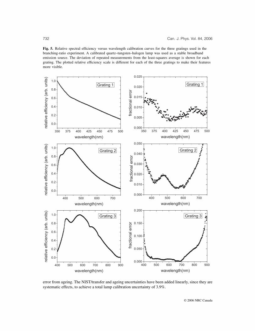
Fig. 5. Relative spectral efficiency versus wavelength calibration curves for the three gratings used in thebranching-ratio experiment. A calibrated quartz–tungsten–halogen lamp was used as a stable broadbandemission source. The deviation of repeated measurements from the least-squares average is shown for eachgrating. The plotted relative efficiency scale is different for each of the three gratings to make their featuresmore visible.

error from ageing. The NIST/transfer and ageing uncertainties have been added linearly, since they aresystematic effects, to achieve a total lamp calibration uncertainty of 3.9%.

© 2006 NRC Canada

Rehse et al. 733

Initial calibrations were conducted on an isolated test bench using various input configurations.These experiments showed that slight differences in the way light is introduced to the monochromatorcould cause large changes in the response. A narrow cone of light entering the monochromator off-axis could lead to underestimates of the efficiency at long wavelengths, where some of the collimatedcalibration light could miss the highly tilted diffraction grating. As well, overfilling the entrance solidangle of the monochromator could lead to stray-light effects that were severely exaggerated whenthe intense long-wavelength continuum of the QTH lamp was present, but were absent in the actualBR measurement. Therefore, great care was taken to block paths by which stray light from the QTHcontinuum source could travel from the entrance slit to the exit slit of the monochromator.

The conclusion drawn from these initial calibrations was that measuring the relative spectral effi-ciency in situ was the best way to perform the calibration. This was done by decoupling one of the fiberbundles from its monochromator and illuminating the decoupled end of the bundle with the QTH lampto transmit its light to the post-acceleration region. Some of the emergent light was collected by theother 80-fiber bundle, and transmitted to the test monochromator. Each grating in the monochromatorwas then scanned over its full wavelength range, and the resulting intensity curve was divided by themanufacturer-provided QTH lamp emission curve to produce a calibration curve of relative efficiencyversus wavelength. The relative efficiency calibration curves of our system for the three gratings used inthe experiment are shown in Fig. 5. Note that the relative efficiencies of the three gratings as presentedin Fig. 5 cannot be compared directly to each other as different scales were used in plotting each gratingto make the spectral dependence visible. Repeated calibrations spanning several months were rescaledwith a least-squares procedure to minimize the residuals summed over wavelength, and showed verylittle change in the relative spectral efficiency of our system. The residuals provided an estimate of theuncertainty in the calibration due to misalignments and (or) changes in the light collection system. Thesedeviations, with typical values less than 3%, are shown in Fig. 5 with their corresponding efficiencycurves.

This calibration procedure most closely reproduced the actual conditions present during the ex-periment, with two minor differences. In the calibration procedure, the light passed through twice thelength of optical fiber compared with that in the actual experiment. With a specified attenuation in thefiber of ∼10 dB/km throughout our wavelength range, the nominal attenuation in the additional lengthof input fiber was estimated to be ∼0.1%. We took 0.2% as a conservative estimate of the maximumuncertainty in the ratio of any two spectral components in our wavelength range due to fiber attenuation.The second difference is that the fraction of light reaching the fibers either directly or by scattering maybe somewhat different in the calibration procedure and in the real experiment. However, any scatteringmust be from the colloidal graphite coating on the aluminum ring that holds the fibers, and the reflectioncoefficient from such a surface is fairly flat over the wavelength range of interest.

To obtain an empirical estimate of the uncertainty in our measurement of the relative detectionefficiency, we examined the relative intensity of all spectral lines that were common to two or morescans, each taken with a different grating. This test exposed any scatter greater than that expected fromthe statistical uncertainty in the calibration shown in Fig. 5. Such excess scatter can only be due tosystematic effects in our calibration. We found that the average magnitude of this excess was ∼3% andit is combined with the fiber attenuation uncertainty to derive a total uncertainty of 3.2%, which appearsin Table 1 as “(systematic) efficiency calibration procedure”.

3.3. Fiber geometry

As described above, two different fiber geometries were used to compensate for anisotropic excita-tion. To test the degree of compensation and the relative collection efficiency, several branching-ratiospectra for the same upper level were obtained with the roles of the two arrays switched. No statisticaldifference in the intensity ratios for different branches was found.

© 2006 NRC Canada

734 Can. J. Phys. Vol. 84, 2006

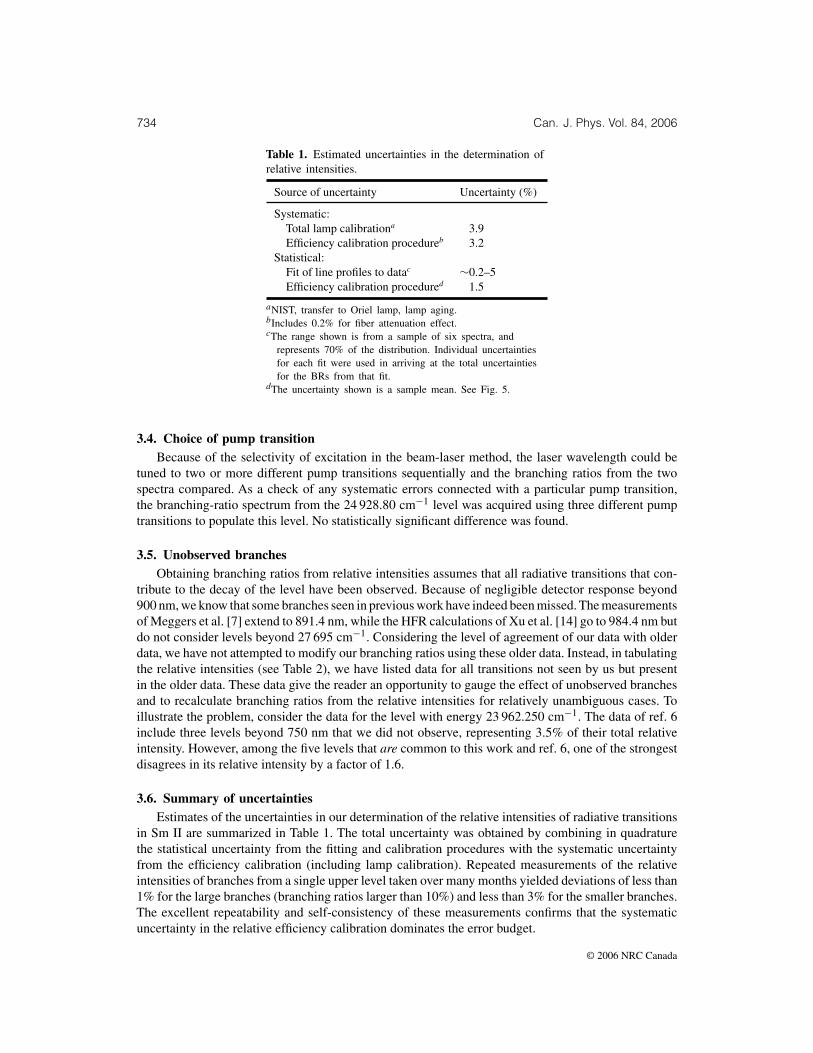
Table 1. Estimated uncertainties in the determination ofrelative intensities.

Source of uncertainty Uncertainty (%)

Systematic:Total lamp calibrationa 3.9Efficiency calibration procedureb 3.2

Statistical:Fit of line profiles to datac ∼0.2–5Efficiency calibration procedured 1.5

aNIST, transfer to Oriel lamp, lamp aging.bIncludes 0.2% for fiber attenuation effect.cThe range shown is from a sample of six spectra, and

represents 70% of the distribution. Individual uncertaintiesfor each fit were used in arriving at the total uncertaintiesfor the BRs from that fit.

dThe uncertainty shown is a sample mean. See Fig. 5.

3.4. Choice of pump transitionBecause of the selectivity of excitation in the beam-laser method, the laser wavelength could be

tuned to two or more different pump transitions sequentially and the branching ratios from the twospectra compared. As a check of any systematic errors connected with a particular pump transition,the branching-ratio spectrum from the 24 928.80 cm−1 level was acquired using three different pumptransitions to populate this level. No statistically significant difference was found.

3.5. Unobserved branchesObtaining branching ratios from relative intensities assumes that all radiative transitions that con-

tribute to the decay of the level have been observed. Because of negligible detector response beyond900 nm, we know that some branches seen in previous work have indeed been missed. The measurementsof Meggers et al. [7] extend to 891.4 nm, while the HFR calculations of Xu et al. [14] go to 984.4 nm butdo not consider levels beyond 27 695 cm−1. Considering the level of agreement of our data with olderdata, we have not attempted to modify our branching ratios using these older data. Instead, in tabulatingthe relative intensities (see Table 2), we have listed data for all transitions not seen by us but presentin the older data. These data give the reader an opportunity to gauge the effect of unobserved branchesand to recalculate branching ratios from the relative intensities for relatively unambiguous cases. Toillustrate the problem, consider the data for the level with energy 23 962.250 cm−1. The data of ref. 6include three levels beyond 750 nm that we did not observe, representing 3.5% of their total relativeintensity. However, among the five levels that are common to this work and ref. 6, one of the strongestdisagrees in its relative intensity by a factor of 1.6.

3.6. Summary of uncertaintiesEstimates of the uncertainties in our determination of the relative intensities of radiative transitions

in Sm II are summarized in Table 1. The total uncertainty was obtained by combining in quadraturethe statistical uncertainty from the fitting and calibration procedures with the systematic uncertaintyfrom the efficiency calibration (including lamp calibration). Repeated measurements of the relativeintensities of branches from a single upper level taken over many months yielded deviations of less than1% for the large branches (branching ratios larger than 10%) and less than 3% for the smaller branches.The excellent repeatability and self-consistency of these measurements confirms that the systematicuncertainty in the relative efficiency calibration dominates the error budget.

© 2006 NRC Canada

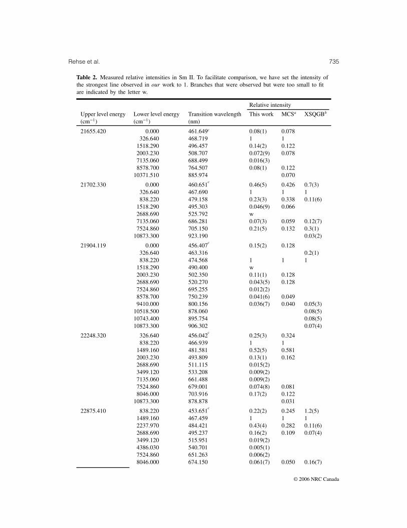
Rehse et al. 735

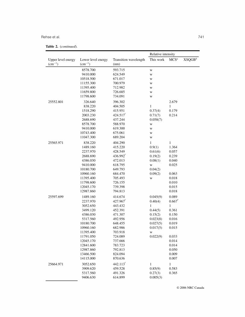
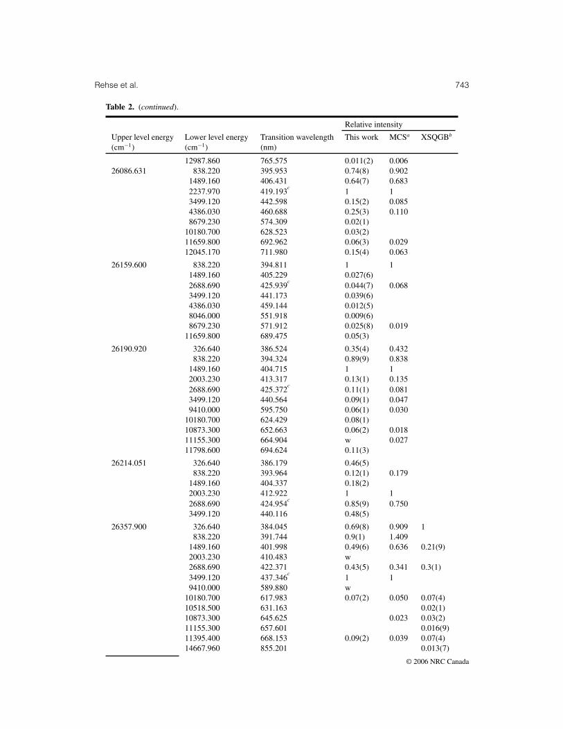
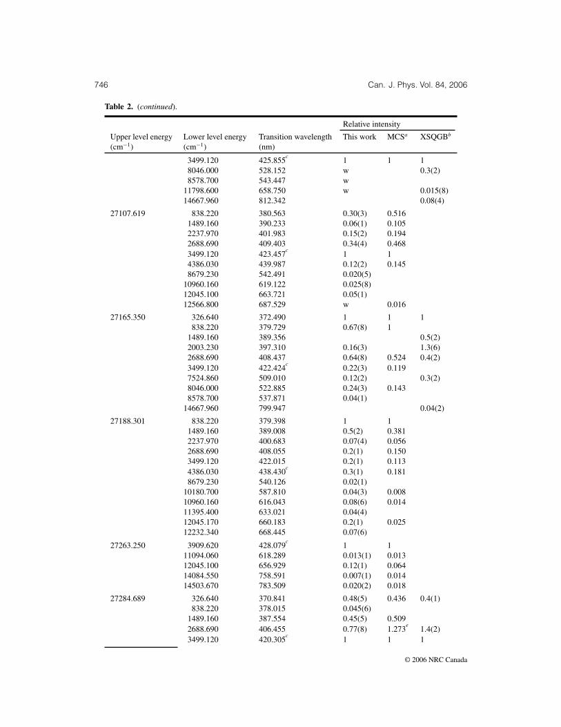
Table 2. Measured relative intensities in Sm II. To facilitate comparison, we have set the intensity ofthe strongest line observed in our work to 1. Branches that were observed but were too small to fitare indicated by the letter w.

Relative intensity

Upper level energy Lower level energy Transition wavelength This work MCSa XSQGBb

(cm−1) (cm−1) (nm)

21655.420 0.000 461.649c 0.08(1) 0.078326.640 468.719 1 1

1518.290 496.457 0.14(2) 0.1222003.230 508.707 0.072(9) 0.0787135.060 688.499 0.016(3)8578.700 764.507 0.08(1) 0.122

10371.510 885.974 0.070

21702.330 0.000 460.651c

0.46(5) 0.426 0.7(3)326.640 467.690 1 1 1838.220 479.158 0.23(3) 0.338 0.11(6)

1518.290 495.303 0.046(9) 0.0662688.690 525.792 w7135.060 686.281 0.07(3) 0.059 0.12(7)7524.860 705.150 0.21(5) 0.132 0.3(1)

10873.300 923.190 0.03(2)

21904.119 0.000 456.407c

0.15(2) 0.128326.640 463.316 0.2(1)838.220 474.568 1 1 1

1518.290 490.400 w2003.230 502.350 0.11(1) 0.1282688.690 520.270 0.043(5) 0.1287524.860 695.255 0.012(2)8578.700 750.239 0.041(6) 0.0499410.000 800.156 0.036(7) 0.040 0.05(3)

10518.500 878.060 0.08(5)10743.400 895.754 0.08(5)10873.300 906.302 0.07(4)

22248.320 326.640 456.042c

0.25(3) 0.324838.220 466.939 1 1

1489.160 481.581 0.52(5) 0.5812003.230 493.809 0.13(1) 0.1622688.690 511.115 0.015(2)3499.120 533.208 0.009(2)7135.060 661.488 0.009(2)7524.860 679.001 0.074(8) 0.0818046.000 703.916 0.17(2) 0.122

10873.300 878.878 0.031

22875.410 838.220 453.651c

0.22(2) 0.245 1.2(5)1489.160 467.459 1 1 12237.970 484.421 0.43(4) 0.282 0.11(6)2688.690 495.237 0.16(2) 0.109 0.07(4)3499.120 515.951 0.019(2)4386.030 540.701 0.005(1)7524.860 651.263 0.006(2)8046.000 674.150 0.061(7) 0.050 0.16(7)

© 2006 NRC Canada

736 Can. J. Phys. Vol. 84, 2006

Table 2. (continued).

Relative intensity

Upper level energy Lower level energy Transition wavelength This work MCSa XSQGBb

(cm−1) (cm−1) (nm)

8679.230 704.221 0.14(1) 0.082 0.3(1)11395.400 870.840 0.03(1)11659.800 891.370 0.02(1)

23177.490 0.000 431.332 0.053(6)326.640 437.498

c0.38(4) 0.681 0.13(8)

838.220 447.517 0.12(1) 0.1601518.290 461.568 1 1 12003.230 472.139 w 0.0622688.690 487.936 w7524.860 638.694 0.013(6) 0.09(5)8578.700 684.800 0.017(8)

10873.300 812.508 0.019 0.013(8)

23260.949 838.220 445.851c

1 11489.160 459.181 0.32(3) 0.2902237.970 475.537 0.048(5) 0.0402688.690 485.956 0.11(1) 0.0853499.120 505.885 0.016(3)8046.000 657.067 0.056(6) 0.0358679.230 685.601 0.13(2) 0.075

12045.170 891.356 0.095

23646.900 1489.160 451.183c

0.59(6) 0.9032237.970 466.964 1 13052.650 485.437 0.17(2) 0.1943499.120 496.194 0.22(2) 0.2744386.030 519.043 w8679.230 667.922 0.079(9) 0.1139406.630 702.040 0.22(3) 0.145

12045.170 861.704 0.03712232.340 875.834 0.048

23659.990 0.000 422.535 0.22(4) 2.273e

326.640 428.451 0.05(3) 0.0801518.290 451.510

c1 1

7135.060 604.979 0.009(5)8578.700 662.890 0.035(9) 0.045

10518.500 760.739 0.02(1) 0.052e

23842.199 326.640 425.131 0.011(2)838.220 434.585

c0.47(5) 0.949

1489.160 447.241 0.52(5) 0.7972003.230 457.769 1 12688.690 472.603 0.21(2) 0.2203499.120 491.430 0.032(4) 0.0247135.060 598.381 0.012(4)7524.860 612.676 w8046.000 632.889 0.016(5)8578.700 654.977 0.036(7) 0.0319410.000 692.704 0.029(9) 0.027

11155.300 787.998 0.017

© 2006 NRC Canada

Rehse et al. 737

Table 2. (continued).

Relative intensity

Upper level energy Lower level energy Transition wavelength This work MCSa XSQGBb

(cm−1) (cm−1) (nm)

11395.400 803.199 0.02711659.800 820.631 0.01011798.600 830.088 0.017

23962.250 326.640 422.971 1 1838.220 432.329

c0.82(8) 0.797

2003.230 455.266 0.89(9) 0.5542688.690 469.936 0.19(2) 0.1628578.700 649.866 0.11(2) 0.047

10743.400 756.287 0.02610873.300 763.793 0.03111798.600 821.896 0.035

24013.561 0.000 416.314 0.36(4) 0.421326.640 422.055 0.09(1)838.220 431.372 0.26(3) 0.474

e

2003.230 454.205 1 1

24194.381 838.220 428.032c

0.57(6) 0.5001489.160 440.304 0.56(6) 4.500

e

2003.230 450.504 1 12688.690 464.863 0.09(1)3499.120 483.068 0.05(1)7135.060 586.027 0.08(3) 0.078

24221.811 326.640 418.377 0.80(9) 1.4321518.290 440.337

c0.63(7) 1.108

2003.230 449.948 1 18578.700 639.082 0.08(1) 0.068

10371.510 721.807 w 0.07011047.300 758.833 w 0.062

24257.369 1489.160 439.086c

1 1 12237.970 454.018 0.14(1) 0.181 1.9(8)3052.650 471.461 0.077(9) 0.047 0.3(1)3499.120 481.602 0.08(1) 0.053 0.15(9)4386.030 503.098 0.013(4)8679.230 641.748 0.045(6) 0.018 0.2(1)9406.630 673.181 0.12(2) 0.075 0.3(1)

10180.700 710.200 0.010(2)10960.160 751.831 w11395.400 777.272 w12045.100 818.628 w 0.06(4)12232.340 831.370 w 0.10(6)12789.810 871.786 w 0.019 0.02(1)12841.600 875.741 w 0.04(2)

24429.520 0.000 409.225 1 1 1326.640 414.771 0.30(3) 0.320 0.000(0)838.220 423.766

c0.68(7) 0.500 0.13(8)

1518.290 436.345 0.32(3) 0.2202003.230 445.780 0.033(4) 0.000(0)2688.690 459.835 0.19(2) 0.090 0.11(6)

© 2006 NRC Canada

738 Can. J. Phys. Vol. 84, 2006

Table 2. (continued).

Relative intensity

Upper level energy Lower level energy Transition wavelength This work MCSa XSQGBb

(cm−1) (cm−1) (nm)

7524.860 591.389 0.021(4)8578.700 630.708 0.065(8) 0.0359410.000 665.616 0.051(6) 0.027 0.10(4)

10371.510 711.143 0.009(2)10518.500 718.657 0.02(1)10743.400 730.466 0.014(3)10873.300 737.466 0.06(4)11155.300 753.133 0.009(3)11798.600 791.490 0.048(8) 0.026

24582.590 326.640 412.154 0.09(1) 0.067838.220 421.034 0.38(4) 0.367

1489.160 432.902c

1 12003.230 442.758 0.16(2) 0.1002688.690 456.620 0.66(7) 0.2613499.120 474.173 0.050(5) 0.0288578.700 624.675 0.033(4) 0.0259410.000 658.902 0.013(2)

10180.700 694.162 0.025(3) 0.00910518.500 710.835 0.005(1)11155.300 744.547 0.024(3)

11659.800 773.614d

0.028(4) 0.017

11798.600 782.013d

0.009

24588.000 2237.970 447.301c

0.71(8) 0.705 0.9(3)3052.650 464.223 1 1 13909.620 483.462 0.08(1) 0.085 0.07(3)4386.030 494.863 0.26(3) 0.193 0.07(4)8679.230 628.410 0.08(3)9406.630 658.520 0.053(7) 0.045 0.03(1)

10214.380 695.527 0.18(2) 0.136 0.27(8)12789.810 847.355 0.02(1)12841.600 851.091 0.05(3)13466.500 898.913 0.03(1)13604.500 910.207 0.011(6)

24685.529 0.000 404.981 1 1326.640 410.412 0.63(8) 0.407838.220 419.216 0.7(1) 0.271

1518.290 431.523 0.11(2)2003.230 440.749

c0.24(5) 0.102

2688.690 454.483 0.44(7) 0.1697135.060 569.627 0.07(2) 0.037

0.031

24689.840 1489.160 430.901 0.51(5) 0.6772237.970 445.272

c1 1

2688.690 454.394 0.79(8) 0.6233499.120 471.773 0.26(3) 0.1624386.030 492.381 0.032(3) 0.0468679.230 624.413 w 0.019

© 2006 NRC Canada

Rehse et al. 739

Table 2. (continued).

Relative intensity

Upper level energy Lower level energy Transition wavelength This work MCSa XSQGBb

(cm−1) (cm−1) (nm)

9410.000 654.276 0.046(5) 0.03810960.160 728.149 0.029(3) 0.02011659.800 767.246 0.00611798.600 775.507 0.01812232.340 802.509 0.01812987.860 854.322 0.018

24848.471 326.640 407.685 0.31(3) 0.075838.220 416.371 0.33(3) 0.083

1489.160 427.974c

1 1e

2003.230 437.605 0.057(6)3499.120 468.267 0.36(4) 0.0637135.060 564.388 0.031(4)7524.860 577.087 0.028(4)8046.000 594.986 0.004(4)8578.700 614.467 0.018(3)9410.000 647.554 0.017(3)

10518.500 697.646 0.007(5)10873.300 715.358 0.009(6)11155.300 730.090 0.030(8)11395.400 743.120 0.019(8)11659.800 758.018 0.029(9)

24928.801 326.640 406.354 1 1838.220 414.983 0.69(7) 1.446

1489.160 426.508 0.47(5) 0.8932003.230 436.072

c0.65(7) 1

2688.690 449.512 0.034(5) 0.0433499.120 466.512 0.14(1) 0.1348578.700 611.448 w 0.032

10180.700 677.866 w 0.07111798.600 761.393 0.021

25055.539 0.000 399.001 0.90(9) 2.027e

326.640 404.271 1 1838.220 412.811 0.057(8) 0.039

1518.290 424.739 0.10(1) 0.0682003.230 433.674 0.11(1) 0.0612688.690 446.965

c0.19(2) 0.122

9410.000 638.983 0.08(2) 0.03910518.500 687.708 0.01610873.300 704.913 0.06(6) 0.018

25175.320 326.640 402.322 1 1838.220 410.779 0.072(9) 0.068

1489.160 422.069 0.041(7)2003.230 431.433 0.042(7)2688.690 444.584

c0.08(1) 0.040

3499.120 461.207 0.025(5)7135.060 554.162 w8046.000 583.633 0.09(1) 0.051

10180.700 666.722 0.10(2) 0.019

© 2006 NRC Canada

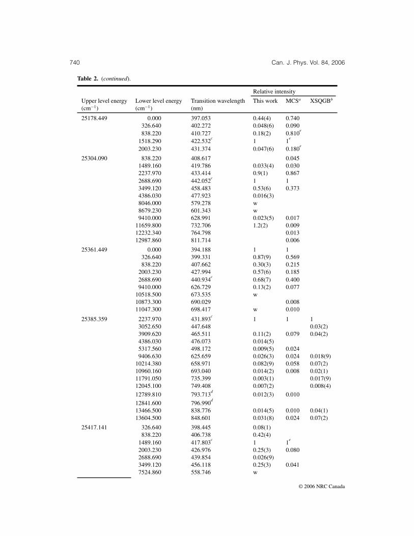
740 Can. J. Phys. Vol. 84, 2006

Table 2. (continued).

Relative intensity

Upper level energy Lower level energy Transition wavelength This work MCSa XSQGBb

(cm−1) (cm−1) (nm)

25178.449 0.000 397.053 0.44(4) 0.740326.640 402.272 0.048(6) 0.090838.220 410.727 0.18(2) 0.810

e

1518.290 422.532c

1 1e

2003.230 431.374 0.047(6) 0.180e

25304.090 838.220 408.617 0.0451489.160 419.786 0.033(4) 0.0302237.970 433.414 0.9(1) 0.8672688.690 442.052

c1 1

3499.120 458.483 0.53(6) 0.3734386.030 477.923 0.016(3)8046.000 579.278 w8679.230 601.343 w9410.000 628.991 0.023(5) 0.017

11659.800 732.706 1.2(2) 0.00912232.340 764.798 0.01312987.860 811.714 0.006

25361.449 0.000 394.188 1 1326.640 399.331 0.87(9) 0.569838.220 407.662 0.30(3) 0.215

2003.230 427.994 0.57(6) 0.1852688.690 440.934

c0.68(7) 0.400

9410.000 626.729 0.13(2) 0.07710518.500 673.535 w10873.300 690.029 0.00811047.300 698.417 w 0.010

25385.359 2237.970 431.893c

1 1 13052.650 447.648 0.03(2)3909.620 465.511 0.11(2) 0.079 0.04(2)4386.030 476.073 0.014(5)5317.560 498.172 0.009(5) 0.0249406.630 625.659 0.026(3) 0.024 0.018(9)

10214.380 658.971 0.082(9) 0.058 0.07(2)10960.160 693.040 0.014(2) 0.008 0.02(1)11791.050 735.399 0.003(1) 0.017(9)12045.100 749.408 0.007(2) 0.008(4)

12789.810 793.713d

0.012(3) 0.010

12841.600 796.990d

13466.500 838.776 0.014(5) 0.010 0.04(1)13604.500 848.601 0.031(8) 0.024 0.07(2)

25417.141 326.640 398.445 0.08(1)838.220 406.738 0.42(4)

1489.160 417.803c

1 1e

2003.230 426.976 0.25(3) 0.0802688.690 439.854 0.026(9)3499.120 456.118 0.25(3) 0.0417524.860 558.746 w

© 2006 NRC Canada

Rehse et al. 741

Table 2. (continued).

Relative intensity

Upper level energy Lower level energy Transition wavelength This work MCSa XSQGBb

(cm−1) (cm−1) (nm)

8578.700 593.715 w9410.000 624.549 w

10518.500 671.017 w11155.300 700.979 w11395.400 712.982 w11659.800 726.685 w11798.600 734.091 w

25552.801 326.640 396.302 2.679838.220 404.505 1 1

1518.290 415.951 0.37(4) 0.1792003.230 424.517

c0.71(7) 0.214

2688.690 437.244 0.058(7)8578.700 588.970 w9410.000 619.300 w

10743.400 675.061 w11047.300 689.204 w

25565.971 838.220 404.290 1 11489.160 415.220 0.9(1) 1.3642237.970 428.549 0.61(6) 0.0572688.690 436.992

c0.19(2) 0.239

4386.030 472.013 0.08(1) 0.0409410.000 618.795 w 0.025

10180.700 649.793 0.04(2)10960.160 684.470 0.09(2) 0.06311395.400 705.493 w 0.01811798.600 726.155 0.01012045.170 739.398 0.01512987.860 794.813 0.018

25597.699 1489.160 414.674 0.045(9) 0.0892237.970 427.967

c0.40(4) 0.667

e

3052.650 443.432 1 13499.120 452.391 0.44(5) 0.3614386.030 471.307 0.15(2) 0.1505317.560 492.956 0.023(8) 0.016

10180.700 648.455 0.027(5) 0.01910960.160 682.986 0.017(5) 0.01511395.400 703.918 w11791.050 724.089 0.022(9) 0.03312045.170 737.666 0.01412841.600 783.723 0.01412987.860 792.813 0.05013466.500 824.094 0.00914115.000 870.636 0.007

25664.971 3052.650 442.113c

1 13909.620 459.528 0.85(9) 0.5835317.560 491.326 0.27(3) 0.3659406.630 614.899 0.005(3)

© 2006 NRC Canada

742 Can. J. Phys. Vol. 84, 2006

Table 2. (continued).

Relative intensity

Upper level energy Lower level energy Transition wavelength This work MCSa XSQGBb

(cm−1) (cm−1) (nm)

10214.380 647.046 0.043(5) 0.01911094.060 686.110 0.21(2) 0.125

e

11791.050 720.578 0.005(4)13466.500 819.550 0.03(1) 0.02013604.500 828.927 w 0.02014084.550 863.289 w 0.024

25790.150 838.220 400.657 0.25(3) 0.3061489.160 411.390 0.60(6) 0.6612237.970 424.470

c1 1

2688.690 432.751 0.11(1) 0.0733499.120 448.486 0.022(3)4386.030 467.069 0.12(1)7524.860 547.335 0.026(3)8679.230 584.260 0.044(5) 0.0359410.000 610.326 0.043(6)

10180.700 640.461 0.015(4)10960.160 674.124 0.09(1)

25939.869 3052.650 436.802c

0.40(4) 0.7043909.620 453.794 1 15317.560 484.776 0.33(3) 0.197

10214.380 635.735 0.022(7)11094.060 673.405 0.13(2) 0.09913466.500 801.488 0.02714084.550 843.271 0.042

25980.320 326.640 389.697 1 1838.220 397.627 0.54(6) 0.600

1489.160 408.195 0.075(8) 0.0812003.230 416.947 0.65(7) 0.5062688.690 429.218

c0.41(4) 0.219

3499.120 444.691 0.048(6) 0.0289410.000 603.322 0.021(4) 0.011

10180.700 632.752 0.09(1) 0.04410873.300 661.761 0.011(4) 0.00711047.300 669.472 0.015(4) 0.00711395.400 685.451 0.022(5) 0.00912566.800 745.311 0.08(2) 0.016

26046.350 3052.650 434.780 0.61(6) 0.6883499.120 443.389

c1 1

4386.030 461.544 0.27(3) 0.1815317.560 482.286 0.006(1)8046.000 555.391 0.003(1)8679.230 575.641 0.004(1)9406.630 600.806 0.006(1)

10180.700 630.118 0.014(2) 0.01412232.340 723.703 0.017(2) 0.008

12789.810 754.137d

0.029(3) 0.014

12841.600 757.095d

0.014

© 2006 NRC Canada

Rehse et al. 743

Table 2. (continued).

Relative intensity

Upper level energy Lower level energy Transition wavelength This work MCSa XSQGBb

(cm−1) (cm−1) (nm)

12987.860 765.575 0.011(2) 0.00626086.631 838.220 395.953 0.74(8) 0.902

1489.160 406.431 0.64(7) 0.6832237.970 419.193

c1 1

3499.120 442.598 0.15(2) 0.0854386.030 460.688 0.25(3) 0.1108679.230 574.309 0.02(1)

10180.700 628.523 0.03(2)11659.800 692.962 0.06(3) 0.02912045.170 711.980 0.15(4) 0.063

26159.600 838.220 394.811 1 11489.160 405.229 0.027(6)2688.690 425.939

c0.044(7) 0.068

3499.120 441.173 0.039(6)4386.030 459.144 0.012(5)8046.000 551.918 0.009(6)8679.230 571.912 0.025(8) 0.019

11659.800 689.475 0.05(3)

26190.920 326.640 386.524 0.35(4) 0.432838.220 394.324 0.89(9) 0.838

1489.160 404.715 1 12003.230 413.317 0.13(1) 0.1352688.690 425.372

c0.11(1) 0.081

3499.120 440.564 0.09(1) 0.0479410.000 595.750 0.06(1) 0.030

10180.700 624.429 0.08(1)10873.300 652.663 0.06(2) 0.01811155.300 664.904 w 0.02711798.600 694.624 0.11(3)

26214.051 326.640 386.179 0.46(5)838.220 393.964 0.12(1) 0.179

1489.160 404.337 0.18(2)2003.230 412.922 1 12688.690 424.954

c0.85(9) 0.750

3499.120 440.116 0.48(5)

26357.900 326.640 384.045 0.69(8) 0.909 1838.220 391.744 0.9(1) 1.409

1489.160 401.998 0.49(6) 0.636 0.21(9)2003.230 410.483 w2688.690 422.371 0.43(5) 0.341 0.3(1)3499.120 437.346

c1 1

9410.000 589.880 w10180.700 617.983 0.07(2) 0.050 0.07(4)10518.500 631.163 0.02(1)10873.300 645.625 0.023 0.03(2)11155.300 657.601 0.016(9)11395.400 668.153 0.09(2) 0.039 0.07(4)14667.960 855.201 0.013(7)

© 2006 NRC Canada

744 Can. J. Phys. Vol. 84, 2006

Table 2. (continued).

Relative intensity

Upper level energy Lower level energy Transition wavelength This work MCSa XSQGBb

(cm−1) (cm−1) (nm)

26505.529 2237.970 411.957 0.036(4) 0.0523052.650 426.267 0.24(2) 0.4483909.620 442.434

c1 1

4386.030 451.963 0.30(3) 0.3035317.560 471.834 0.084(9) 0.066

10960.160 643.101 0.010(2) 0.00811791.050 679.415 0.045(5) 0.03312789.810 728.890 w 0.00612841.600 731.653 0.004(2)13466.500 766.717 w 0.00713604.500 774.919 0.009(3) 0.010

14084.550 804.868d

0.043(7) 0.014

14115.000 806.846d

0.016

26540.119 3052.650 425.639c

1 13909.620 441.758 0.16(2) 0.1815317.560 471.065 0.045(5) 0.029

10214.380 612.360 0.014(1) 0.01011094.060 647.235 0.063(7) 0.02111791.050 677.822 0.020(2) 0.01012789.810 727.056 0.004(1)13604.500 772.847 0.014(2) 0.01414084.550 802.633 0.019(2) 0.01114503.670 830.582 0.044(5) 0.019

26565.609 1489.160 398.668 1 12237.970 410.939 0.58(6) 0.5543052.650 425.178

c0.45(5) 0.338

3499.120 433.408 0.050(6)4386.030 450.739 0.028(5)5317.560 470.500 0.032(5)8046.000 539.819 0.041(7)8679.230 558.930 0.024(6)

10960.160 640.625 0.11(2) 0.01611395.400 659.005 w11791.050 676.652 0.07(2) 0.01912045.100 688.495 0.06(2)12232.340 697.485 0.05(2)12789.810 725.711 0.10(3) 0.012

26599.080 0.000 375.846 0.59(7) 0.563838.220 388.076 1 1

1518.290 398.599 0.24(3) 0.1882003.230 406.458 0.84(9) 1.750

e

2688.690 418.110c

0.77(8) 0.6637135.060 513.626 0.06(2) 0.000

10518.500 621.696 0.10(5) 0.00010743.400 630.514 0.10(5) 0.01610873.300 635.723 0.16(5) 0.03611047.300 642.836 0.22(6) 0.02811798.600 675.467 0.09(7) 0.021

e

© 2006 NRC Canada

Rehse et al. 745

Table 2. (continued).

Relative intensity

Upper level energy Lower level energy Transition wavelength This work MCSa XSQGBb

(cm−1) (cm−1) (nm)

26723.869 326.640 378.720 0.35(4) 0.485838.220 386.205 1 1

2003.230 404.406 0.46(5) 0.3642688.690 415.940

c0.37(4) 0.152

26820.811 1489.160 394.651 0.71(7) 0.6172237.970 406.673 1 13052.650 420.612 1 0.8153499.120 428.665

c0.46(5) 0.432

4386.030 445.611 0.13(1) 0.1115317.560 464.916 0.035(6)9406.630 574.086 0.033(8)

10180.700 600.792 0.035(9)10960.160 630.317 0.07(1) 0.03611791.050 665.163 w 0.02512789.810 712.511 w 0.028

26828.289 3052.650 420.480 0.022(3) 0.042 0.14(5)3909.620 436.203 0.54(5) 0.675 0.04(1)4386.030 445.463 1 1 15317.560 464.754 0.15(2) 0.0759406.630 573.839 0.008(4)

10214.380 601.739 0.015 0.02(1)11791.050 664.832 0.009(5)12789.810 712.132 0.006(3)13466.500 748.197 0.67(9) 0.02213604.500 756.005 0.25(5) 0.010 0.010(5)

14084.550 784.483d

0.8(1) 0.008

14115.000 786.362d

0.016 0.002(1)15897.540 914.599 0.003(1)16615.500 978.896 0.04(1)

26880.600 3052.650 419.557 0.020(2)3909.620 435.210

c0.80(8) 0.789

4386.030 444.427 1 15317.560 463.627 0.18(2) 0.1278679.230 549.257 0.012(2)9406.630 572.122 0.018(3)

10960.160 627.950 0.015(2) 0.01411791.050 662.527 0.014(2) 0.00812045.100 673.876 0.003(1)12841.600 712.105 0.013(2)13466.500 745.279 0.026(4)14084.550 781.276 0.01114115.000 783.140 0.043(6) 0.014

26974.670 326.640 375.156 0.37(4) 0.762838.220 382.499 0.34(4)

1489.160 392.269 0.31(3) 0.429 0.9(6)2003.230 400.344 0.90(9) 1.333 6.4(38)2688.690 411.644 0.74(8) 0.905 2.4(14)

© 2006 NRC Canada

746 Can. J. Phys. Vol. 84, 2006

Table 2. (continued).

Relative intensity

Upper level energy Lower level energy Transition wavelength This work MCSa XSQGBb

(cm−1) (cm−1) (nm)

3499.120 425.855c

1 1 18046.000 528.152 w 0.3(2)8578.700 543.447 w

11798.600 658.750 w 0.015(8)14667.960 812.342 0.08(4)

27107.619 838.220 380.563 0.30(3) 0.5161489.160 390.233 0.06(1) 0.1052237.970 401.983 0.15(2) 0.1942688.690 409.403 0.34(4) 0.4683499.120 423.457

c1 1

4386.030 439.987 0.12(2) 0.1458679.230 542.491 0.020(5)

10960.160 619.122 0.025(8)12045.100 663.721 0.05(1)12566.800 687.529 w 0.016

27165.350 326.640 372.490 1 1 1838.220 379.729 0.67(8) 1

1489.160 389.356 0.5(2)2003.230 397.310 0.16(3) 1.3(6)2688.690 408.437 0.64(8) 0.524 0.4(2)3499.120 422.424

c0.22(3) 0.119

7524.860 509.010 0.12(2) 0.3(2)8046.000 522.885 0.24(3) 0.1438578.700 537.871 0.04(1)

14667.960 799.947 0.04(2)

27188.301 838.220 379.398 1 11489.160 389.008 0.5(2) 0.3812237.970 400.683 0.07(4) 0.0562688.690 408.055 0.2(1) 0.1503499.120 422.015 0.2(1) 0.1134386.030 438.430

c0.3(1) 0.181

8679.230 540.126 0.02(1)10180.700 587.810 0.04(3) 0.00810960.160 616.043 0.08(6) 0.01411395.400 633.021 0.04(4)12045.170 660.183 0.2(1) 0.02512232.340 668.445 0.07(6)

27263.250 3909.620 428.079c

1 111094.060 618.289 0.013(1) 0.01312045.100 656.929 0.12(1) 0.06414084.550 758.591 0.007(1) 0.01414503.670 783.509 0.020(2) 0.018

27284.689 326.640 370.841 0.48(5) 0.436 0.4(1)838.220 378.015 0.045(6)

1489.160 387.554 0.45(5) 0.5092688.690 406.455 0.77(8) 1.273

e1.4(2)

3499.120 420.305c

1 1 1

© 2006 NRC Canada

Rehse et al. 747

Table 2. (continued).

Relative intensity

Upper level energy Lower level energy Transition wavelength This work MCSa XSQGBb

(cm−1) (cm−1) (nm)

8046.000 519.642 0.015(4) 0.02(1)11047.300 615.692 0.033(8) 0.013 0.02(1)11155.300 619.815 0.043(8) 0.00911395.400 629.181 0.06(1) 0.045 0.015(8)11659.800 639.828 0.043(9)11798.600 645.562 0.06(1) 0.013 0.08(2)12566.800 679.258 0.05(1) 0.01312987.860 699.263 0.013(7)14667.960 792.380 0.010(5)16078.000 892.059 0.006(3)17005.300 972.534 0.014(7)

27309.730 1489.160 387.178 1 12237.970 398.742 0.48(5) 0.4633052.650 412.135 0.72(8) 0.5134386.030 436.107

c0.50(5) 0.275

5317.560 454.580 0.11(1) 0.03610180.700 583.643 0.11(2)10960.160 611.468 0.15(3)12232.340 663.062 0.11(4) 0.018

12789.810 688.519d

0.46(8) 0.034

12841.600 690.984d

0.018

27464.199 838.220 375.466 0.057(8)1489.160 384.876 0.18(2) 0.865 1.1(5)2237.970 396.301 1 1.1(5)2688.690 403.510 0.93(9) 1 13499.120 417.156

c0.55(6) 0.554 0.3(2)

4386.030 433.189 0.028(4)8679.230 532.193 0.023(5)9410.000 553.734 0.014(4)

10180.700 578.426 0.2(1)10873.300 602.573 0.12(7)10960.160 605.745 0.14(8)11395.400 622.152 0.15(9)11659.800 632.560 0.07(1) 0.024 0.011(7)12045.100 648.370 0.030(9) 0.3(1)12232.340 656.337 0.05(7) 0.08(5)12566.800 671.073 w15242.950 818.022 0.03(2)

27695.961 3909.620 420.291c

0.078(8) 0.295 0.12(4)5317.560 446.734 1 1 1

11094.060 602.174 0.005(1) 0.013(4)11791.050 628.563 0.006(3)13466.500 702.574 0.003(2)14084.550 734.475 0.010(5)14503.670 757.810 0.017(3) 0.009 0.017(5)16615.500 902.242 0.002(1)17391.890 970.224 0.04(1)

© 2006 NRC Canada

748 Can. J. Phys. Vol. 84, 2006

Table 2. (continued).

Relative intensity

Upper level energy Lower level energy Transition wavelength This work MCSa XSQGBb

(cm−1) (cm−1) (nm)

28072.330 838.220 367.082 1 11489.160 376.071 0.64(7) 0.8642688.690 393.843 w 0.0133499.120 406.832 0.31(3) 0.3234386.030 422.066

c0.62(6) 0.336

8046.000 499.203 0.09(1) 0.0328679.230 515.504 0.24(3) 0.164

11395.400 599.465 0.04(1) 0.01112045.170 623.768 0.01312566.800 644.753 0.00313777.050 699.339 0.006

28151.400 2237.970 385.791 0.45(6) 0.6493052.650 398.314 1 13909.620 412.395 0.81(9) 0.9594386.030 420.662 0.57(7) 0.3655317.560 437.824

c0.9(1) 1.189

11791.050 611.065 0.12(2) 0.06113604.500 687.242 0.11(3) 0.03614115.000 712.237 w 0.016

28191.961 1489.160 374.387 12237.970 385.188 0.38(5) 13499.120 404.861 0.11(2) 0.5004386.030 419.945 0.37(4) 0.6435317.560 437.047

c0.13(3) 0.107

8679.230 512.344 w9406.630 532.183 0.06(1)

10180.700 555.054 0.04(1)10960.160 580.162 w 0.02112045.100 619.147 w12232.340 626.408 w12789.810 649.081 0.21(4) 0.069

28256.320 838.220 364.619 0.011(1)1489.160 373.486 0.039(4)2237.970 384.235 0.15(2) 0.2702688.690 391.009 0.063(8) 0.0903499.120 403.809 0.11(1) 0.1504386.030 418.813

c1 1

8679.230 510.659 0.027(4)11659.800 602.370 0.018(5)11798.600 607.450 0.015(5)12232.340 623.892 0.020(6)12566.800 637.192 0.024(7)13777.050 690.452 0.025(9) 0.010

28445.430 838.220 362.121 1 11489.160 370.866 0.76(8) 0.5472237.970 381.463 0.24(3) 0.2472688.690 388.138 0.37(4) 0.265

© 2006 NRC Canada

Rehse et al. 749

Table 2. (continued).

Relative intensity

Upper level energy Lower level energy Transition wavelength This work MCSa XSQGBb

(cm−1) (cm−1) (nm)

3499.120 400.748 0.27(3) 0.2764386.030 415.521

c0.64(7) 0.329

7524.860 477.865 w8046.000 490.073 0.18(5) 0.0248679.230 505.773 0.36(5) 0.038

11659.800 595.583 0.10(4) 0.01515242.950 757.225 0.014

28540.119 2237.970 380.089 0.41(5) 0.3203052.650 392.239 1 13909.620 405.886 0.27(3) 0.1764386.030 413.892 0.06(2) 0.0205317.560 430.495

c0.23(3) 0.128

9406.630 522.499 0.024(5)10214.380 545.529 0.020(7)10960.160 568.672 0.06(1) 0.01211791.050 596.883 0.05(1) 0.01412045.100 606.079 w12841.600 636.827 0.06(2) 0.00913466.500 663.228 0.13(2) 0.01613604.500 669.356 0.14(2) 0.028

28725.529 1489.160 367.052 0.09(1)2237.970 377.429 0.074(9)3052.650 389.406 0.35(4) 0.4943499.120 396.298 0.36(4)4386.030 410.739 1 1

e

5317.560 427.085c

0.48(5) 0.1858679.230 498.707 w9406.630 517.484 w

10960.160 562.737 w11395.400 576.870 w12789.810 627.348 w13777.050 668.780 w 0.021

28913.990 1489.160 364.529 0.29(3) 0.3002237.970 374.762 0.27(3) 0.4003052.650 386.568 0.040(5) 0.0673499.120 393.359 0.19(2)4386.030 407.583 0.64(6) 0.6755317.560 423.674

c1 1

8679.230 494.062 0.041(5)9406.630 512.484 0.064(8) 0.042

13777.050 660.453 0.08(1) 0.079

28997.141 1489.160 363.427 1 12237.970 373.597 0.48(5) 0.4713052.650 385.329 0.05(2)5317.560 422.186

c0.028(6)

8046.000 477.168 w8679.230 492.039 0.04(1) 0.022

© 2006 NRC Canada

750 Can. J. Phys. Vol. 84, 2006

Table 2. (concluded).

Relative intensity

Upper level energy Lower level energy Transition wavelength This work MCSa XSQGBb

(cm−1) (cm−1) (nm)

9406.630 510.309 0.15(4) 0.076

12045.170 589.739d

0.030(9) 0.013

12232.340 596.323d

0.00712789.810 616.834 0.013(4) 0.00415897.540 763.172 0.003

29387.869 1489.160 358.337 0.32(6) 0.5852237.970 368.221 0.11(3)3499.120 386.159 0.09(3)5317.560 415.333

c1 1

8679.230 482.756 0.032(7)13777.050 640.404 0.07(2) 0.017

aRefs. 6 and 7. The uncertainties are stated to be in the range of 15–25%.bRef. 14. The tabulated relative intensities have been derived from the calculated transition probabilities.cTransition pumped by laser.dUnresolved lines in this work.eBlended line in Refs. 6 and 7.

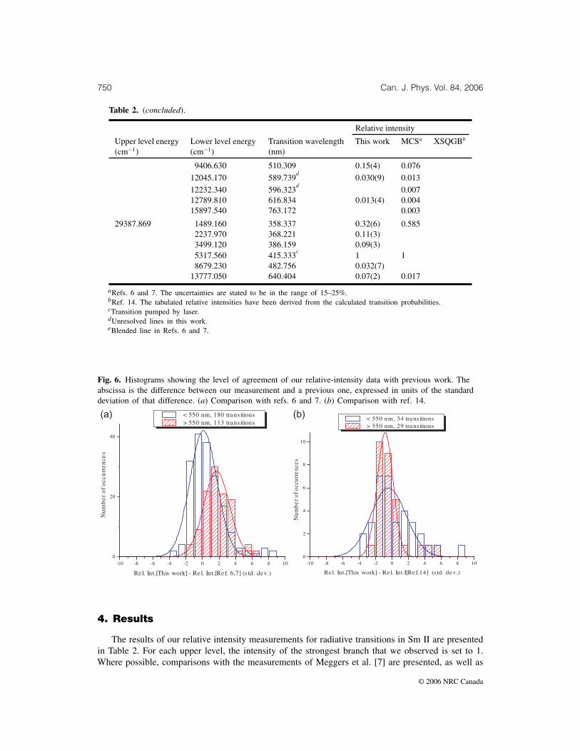
Fig. 6. Histograms showing the level of agreement of our relative-intensity data with previous work. Theabscissa is the difference between our measurement and a previous one, expressed in units of the standarddeviation of that difference. (a) Comparison with refs. 6 and 7. (b) Comparison with ref. 14.

4. Results

The results of our relative intensity measurements for radiative transitions in Sm II are presentedin Table 2. For each upper level, the intensity of the strongest branch that we observed is set to 1.Where possible, comparisons with the measurements of Meggers et al. [7] are presented, as well as

© 2006 NRC Canada

Rehse et al. 751

with HFR calculations by Xu et al., [14] taken from the DREAM database [15]. An overall picture ofthe comparison is given in Fig. 6, which displays histograms of the differences between our results andthose of Meggers et al. [6, 7] and Xu et al. [14]; these differences are in units of the standard deviationof the difference. Also included are best-fit Gaussian distributions. In Fig. 6a (Meggers et al.), we havesomewhat arbitrarily used the upper limit of their stated 15–25% accuracy. The agreement is quitegood for transitions with wavelengths λ < 550 nm, but there is a systematic shift for transitions withλ > 550 nm. Figure 6b (Xu et al.) shows better agreement in both wavelength ranges λ < 550 nm.The presence of a systematic shift for λ > 550 nm in only one of the comparisons suggests that thedisagreement for this wavelength range is not due to a systematic error in our efficiency calibration.A number of interesting examples that exhibit the advantages of this new method can be drawn fromTable 2. In the case of the 28 997.14 cm−1 level, the 385.33 nm transition to the 3 052.65 cm−1 levelhad never been experimentally observed before, and its relative intensity cannot be determined frommeasurements on a discharge lamp light source, because it is completely overlapped by a strong line inSm I at 385.33 nm.

As another example, the transition at 396.301 nm was assigned by Meggers et al. [6, 7] to the upperenergy level 25 552.801 cm−1, and was the strongest branch from that level, with the lower level at326.640 cm−1. We saw no trace of this line in the spectrum for this upper level, but it appeared in ourspectra as the strongest branch from the level at 27 464.199 cm−1, and must have 2 237.970 cm−1 as itslower level. The difference in transition energy for these two assignments corresponds to a wavelengthdifference of only 0.001 nm. Nevertheless, highly selective laser excitation removes any ambiguityabout the correct assignment. This assignment agrees with the predictions of Xu et al. [14].

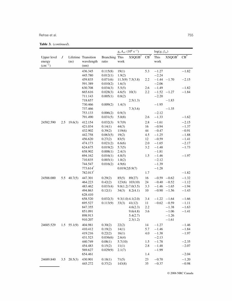
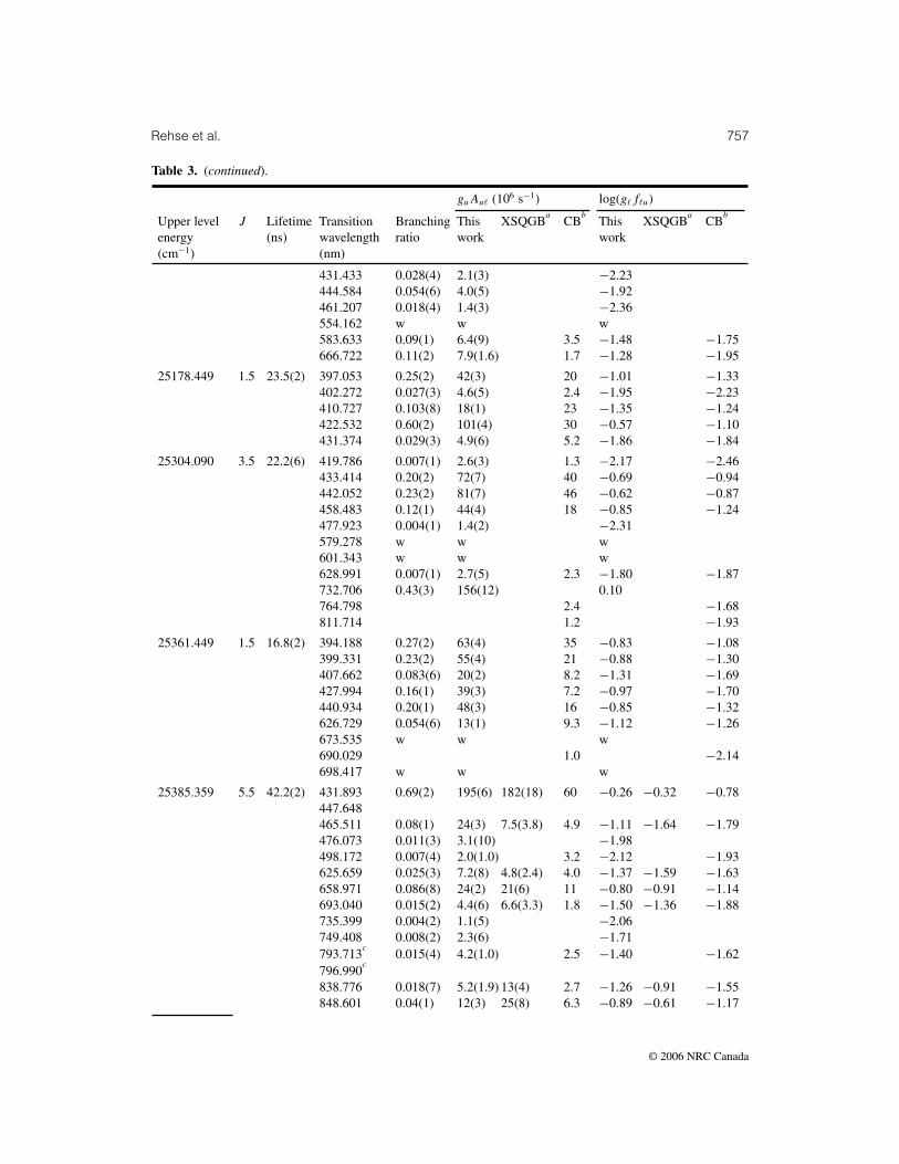
Tables 3 and 4 present our BR measurements, along with spontaneous-emission transition probabil-ities guAu� and log g�f�u values obtained by combining the BRs with our previously measured lifetimedata [16]. Table 3 includes comparisons with the data of Xu et al. [14] and Corliss and Bozman [8]while Table 4 includes comparisons with the data of Saffman and Whaling [9]. Transitions are identifiedby the upper-level energy, angular momentum J and air wavelength, taken from the earlier references.When transitions not previously attributed to the upper level were observed, the air wavelengths werecalculated from tabulated level energies [11, 12]. The transition probabilities and the oscillator strengthswere calculated using the well-known formulas for electric dipole transitions

Au� = Ru�

τu

(3)

g�f�u = 1

0.66 702σ 2u�

guAu� (4)

where Au� is the transition probability, Ru� is the branching ratio, τu is the upper-state lifetime, f�u isthe absorption oscillator strength, gu and g� are the 2J + 1 statistical weights of the upper and lowerlevels, respectively, and σu� is the transition wave number (in cm−1) [24].

5. Conclusions

We have measured 608 log (g�f�u) values for Sm II transitions over the wavelength range 358–876 nm. These transitions originate from 69 upper levels in the range 21 655–29 388 cm−1. Thelog (g�f�u) values were obtained by combining measured relative intensities with previously measuredradiative lifetimes. The uncertainties arose principally from systematics of the efficiency calibration ofthe optical detection system (7.1%), with smaller statistical contributions. Highly selective laser ex-citation of only a single upper level (usually a single hyperfine level) produces a simple fluorescencespectrum, removing any ambiguity in the assignment of transitions to a pair of energy levels.

© 2006 NRC Canada

752 Can. J. Phys. Vol. 84, 2006

Table 3. Transition probabilities and oscillator strengths derived from branching-ratio and lifetime data.Data from this work are compared with those of refs. 8 and 14. Branches that were observed but were toosmall to fit are indicated by the letter w. The issue of unobserved branches is discussed in the text.

guAu� (106 s−1) log(g�f�u)

Upper levelenergy(cm−1)

J Lifetime(ns)

Transitionwavelength(nm)

Branchingratio

Thiswork

XSQGBa

CBb

Thiswork

XSQGBa

CBb

21655.420 0.5 51.9(5) 461.649 0.051(6) 2.0(2) 0.34 −2.20 −2.96468.719 0.69(2) 26.5(8) 6.6 −1.06 −1.66496.457 0.103(9) 4.0(4) 1.1 −1.83 −2.39508.707 0.054(5) 2.1(2) 0.75 −2.09 −2.53688.499 0.016(3) 0.6(1) −2.36764.507 0.09(1) 3.5(4) 2.0 −1.52 −1.76885.974

21702.330 1.5 40.2(2) 460.651 0.21(2) 21(2) 26(8) 3.5 −1.18 −1.14 −1.96467.690 0.47(3) 46(3) 39(12) 12 −0.82 −0.94 −1.39479.158 0.11(1) 11(1) 4.4(2.2) 4.3 −1.43 −1.86 −1.83495.303 0.023(4) 2.3(4) 1.1 −2.08 −2.39525.792 w w w686.281 0.05(2) 4.9(1.7) 6.8(3.4) 1.5 −1.46 −1.38 −1.96705.150 0.14(3) 14(3) 17(5) 3.7 −0.97 −0.96 −1.56923.190 2.2(1.1) −1.64

21904.119 1.5 70.8(6) 456.407 0.098(8) 5.5(5) 0.73 −1.76 −2.64463.316 6.2(3.1) −1.75474.568 0.6920(2) 39(1) 31(9) 9.1 −0.88 −1.04 −1.51

21904.119 1.5 70.8(6) 490.400 w w w502.350 0.079(7) 4.5(4) 1.6 −1.77 −2.22520.270 0.033(3) 1.9(2) 1.7 −2.12 −2.17695.255 0.013(2) 0.7(1) −2.29750.239 0.045(5) 2.5(3) 1.0 −1.67 −2.05800.156 0.042(8) 2.4(4) 2.8(1.4) 0.95 −1.64 −1.64 −2.04878.060 4.6(2.3) −1.37895.754 4.5(2.3) −1.36906.302 4.2(2.1) −1.38

22248.320 2.5 33.8(9) 456.042 0.107(8) 19(2) 3.2 −1.23 −2.00466.939 0.43(2) 77(4) 10 −0.60 −1.48481.581 0.23(2) 41(3) 9.3 −0.85 −1.49493.809 0.058(5) 10.3(9) 3.5 −1.42 −1.90511.115 0.007(1) 1.3(2) −2.30533.208 0.004(1) 0.8(2) −2.47661.488 0.006(1) 1.0(2) −2.19679.001 0.046(4) 8.2(7) 2.7 −1.24 −1.73703.916 0.108(8) 19(2) 4.3 −0.85 −1.49878.878 1.3 −1.81

22875.410 3.5 39.9(1) 453.651 0.099(8) 20(2) 72(22) 4.3 −1.21 −0.70 −1.88467.459 0.46(2) 93(4) 64(19) 27 −0.52 −0.73 −1.05484.421 0.21(1) 41(3) 7.3(3.6) 8.1 −0.84 −1.64 −1.54495.237 0.079(6) 16(1) 4.7(2.4) 4.1 −1.23 −1.80 −1.82515.951 0.010(1) 2.0(2) −2.10540.701 0.003(1) 0.5(1) −2.66651.263 0.004(1) 0.8(2) −2.29

© 2006 NRC Canada

Rehse et al. 753

Table 3. (continued).

guAu� (106 s−1) log(g�f�u)

Upper levelenergy(cm−1)

J Lifetime(ns)

Transitionwavelength(nm)

Branchingratio

Thiswork

XSQGBa

CBb

Thiswork

XSQGBa

CBb

674.150 0.041(4) 8.2(7) 15(5) 2.8 −1.25 −1.05 −1.72704.221 0.095(7) 19(1) 28(8) 5.2 −0.85 −0.74 −1.42870.840 3.0(1.5) 3.2 −1.55 −1.44891.370 2.4(1.2) −1.63

23177.490 1.5 48.0(4) 431.332 0.032(3) 2.6(3) −2.13437.498 0.23(2) 19(1) 7.3(3.7) 5.5 −1.26 −1.73 −1.80447.517 0.076(7) 6.3(5) 1.3 −1.72 −2.42461.568 0.64(2) 53(2) 59(18) 8.4 −0.77 −0.78 −1.57472.139 w w 0.81 w −2.57487.936 w w w638.694 0.011(5) 0.9(4) 7.0(3.5) −2.25 −1.44684.800 0.016(7) 1.3(6) −2.04812.508 1.4(7) 0.65 −1.95 −2.19

23260.949 3.5 53.8(6) 445.851 0.55(2) 82(3) 18 −0.61 −1.27459.181 0.18(1) 27(2) −1.06475.537 0.029(3) 4.3(4) 1.1 −1.84 −2.42485.956 0.064(5) 9.5(8) 2.6 −1.47 −2.04505.885 0.010(2) 1.5(2) −2.24657.067 0.046(4) 6.8(7) 3.4 −1.35 −1.66685.601 0.11(1) 17(2) 4.4 −0.92 −1.51891.356 7.8 −1.03

23646.900 4.5 42.5(1) 451.183 0.24(2) 56(4) 11 −0.77 −1.47466.964 0.41(2) 97(5) 13 −0.50 −1.38485.437 0.073(6) 17(1) 3.8 −1.22 −1.87496.194 0.098(8) 23(2) 7.7 −1.07 −1.54519.043 w w w667.922 0.047(4) 11(1) 4.3 −1.13 −1.54702.040 0.14(1) 32(3) 6.4 −0.63 −1.33861.704 2.0 −1.66875.834 2.8 −1.48

23659.990 0.5 31.8(5) 422.535 0.15(2) 9.6(1.2) −1.59428.451 0.04(2) 2.3(1.1) −2.20451.510 0.74(3) 46(2) −0.85604.979 0.009(5) 0.5(3) −2.52662.890 0.038(9) 2.4(6) −1.81760.739 0.03(2) 1.7(1.0) −1.83

23842.199 2.5 33.6(3) 425.131 0.004(1) 0.8(2) −2.68434.585 0.19(1) 34(2) 11 −1.02 −1.49447.241 0.22(2) 39(3) 9.8 −0.94 −1.53457.769 0.424(2) 76(4) 13 −0.62 −1.40472.603 0.094(7) 17(1) 4.2 −1.25 −1.85491.430 0.015(2) 2.6(3) 0.47 −2.02 −2.77598.381 0.007(2) 1.2(4) −2.18612.676 w w w632.889 0.009(3) 1.6(5) −2.01654.977 0.022(4) 3.9(7) 1.1 −1.61 −2.14

© 2006 NRC Canada

754 Can. J. Phys. Vol. 84, 2006

Table 3. (continued).

guAu� (106 s−1) log(g�f�u)

Upper levelenergy(cm−1)

J Lifetime(ns)

Transitionwavelength(nm)

Branchingratio

Thiswork

XSQGBa

CBb

Thiswork

XSQGBa

CBb

692.704 0.019(5) 3.3(9) 1.2 −1.62 −2.07787.998803.199 1.4 −1.87820.631830.088 0.91 −2.03

23962.250 1.5 22.54(6) 422.971 0.31(2) 56(3) 15 −0.82 −1.39432.329 0.26(2) 47(3) 12 −0.88 −1.46455.266 0.30(2) 54(3) 9.1 −0.78 −1.55469.936 0.065(5) 11.5(9) 4.0 −1.42 −1.88649.866 0.055(7) 9.7(1.2) 2.3 −1.21 −1.83756.287763.793 1.9 −1.78821.896 2.3 −1.63

24013.561 1.5 69.1(2) 416.314 0.20(2) 11.5(9) −1.52422.055 0.048(6) 2.8(4) −2.13431.372 0.15(1) 8.7(7) −1.62454.205 0.60(2) 35(1) −0.97

24194.381 2.5 162.8(7) 428.032 0.23(2) 8.6(6) 1.9 −1.63 −2.27440.304 0.23(2) 8.6(6) 18 −1.60 −1.27450.504 0.43(2) 15.8(8) 4.1 −1.32 −1.90464.863 0.038(6) 1.4(2) −2.35483.068 0.023(6) 0.8(2) −2.54586.027 0.04(1) 1.6(5) 0.89 −2.07 −2.34

24221.811 0.5 15.5(2) 418.377 0.30(2) 39(3) 12 −0.99 −1.52440.337 0.25(2) 32(2) 9.4 −1.03 −1.56449.948 0.41(2) 52(3) 8.6 −0.80 −1.58639.082 0.044(7) 5.7(9) 1.7 −1.46 −1.98721.807 w w w758.833 w w w

24257.369 4.5 46.6(3) 439.086 0.63(2) 135(4) 44(13) 37 −0.41 −0.91 −0.97454.018 0.088(8) 19(2) 89(27) 7.0 −1.23 −0.58 −1.66471.461 0.052(5) 11(1) 14(4) 2.9 −1.43 −1.34 −2.01481.602 0.058(6) 12(1) 7.5(3.8) 3.3 −1.37 −1.60 −1.93503.098 0.009(3) 1.9(7) −2.13641.748 0.041(5) 8.8(1.1) 15(5) 2.0 −1.26 −1.05 −1.91673.181 0.12(1) 25(3) 22(7) 8.8 −0.78 −0.84 −1.22710.200 0.010(2) 2.2(4) −1.79751.831 w w w777.272 w w w818.628 w w 5.1(2.6) w −1.32831.370 w w 8.6(4.3) w −1.08871.786 w w 1.9(9) 3.4 w −1.70 −1.42875.741 w w 3.2(1.6) w −1.47

24429.520 1.5 24.7(1) 409.225 0.34(2) 55(3) 62(19) 23 −0.86 −0.88 −1.23414.771 0.104(8) 17(1) 7.4 −1.36 −1.72423.766 0.24(2) 39(2) 8.4(4.2) 12 −0.98 −1.72 −1.50

© 2006 NRC Canada

Rehse et al. 755

Table 3. (continued).

guAu� (106 s−1) log(g�f�u)

Upper levelenergy(cm−1)

J Lifetime(ns)

Transitionwavelength(nm)

Branchingratio

Thiswork

XSQGBa

CBb

Thiswork

XSQGBa

CBb

436.345 0.115(8) 19(1) 5.3 −1.27 −1.82445.780 0.012(1) 1.9(2) −2.24459.835 0.071(6) 11.5(9) 7.5(3.8) 2.2 −1.44 −1.70 −2.15591.389 0.010(2) 1.6(3) −2.06630.708 0.034(3) 5.5(5) 2.6 −1.49 −1.82665.616 0.028(3) 4.6(5) 10(3) 2.2 −1.52 −1.27 −1.84711.143 0.005(1) 0.8(2) −2.20718.657 2.5(1.3) −1.83730.466 0.009(2) 1.4(3) −1.95737.466 7.3(3.6) −1.35753.133 0.006(2) 0.9(3) −2.12791.490 0.031(5) 5.0(8) 2.6 −1.33 −1.62

24582.590 2.5 19.6(3) 412.154 0.032(3) 9.7(9) 2.8 −1.61 −2.15421.034 0.14(1) 44(3) 16 −0.94 −1.37432.902 0.39(2) 119(6) 44 −0.47 −0.91442.758 0.063(5) 19(2) 4.5 −1.25 −1.88456.620 0.27(2) 83(5) 12 −0.59 −1.41474.173 0.021(2) 6.6(6) 2.0 −1.65 −2.17624.675 0.019(2) 5.7(5) 3.2 −1.48 −1.73658.902 0.008(1) 2.4(3) −1.81694.162 0.016(1) 4.8(5) 1.5 −1.46 −1.97710.835 0.003(1) 1.0(2) −2.12744.547 0.016(2) 4.9(6) −1.39773.614

c0.019(2)5.9(7) −1.28

782.013c

1.7 −1.82

24588.000 5.5 40.7(5) 447.301 0.29(2) 85(5) 89(27) 16 −0.59 −0.62 −1.32464.223 0.42(2) 123(6) 103(10) 24 −0.40 −0.52 −1.12483.462 0.033(4) 9.8(1.2) 7.0(3.5) 3.3 −1.46 −1.65 −1.94494.863 0.12(1) 34(3) 8.2(4.1) 10 −0.90 −1.56 −1.43628.410658.520 0.032(3) 9.3(1.0) 4.1(2.0) 3.4 −1.22 −1.64 −1.66695.527 0.113(9) 33(3) 41(12) 11 −0.62 −0.59 −1.11847.355 4.6(2.3) 2.2 −1.38 −1.63851.091 9.6(4.8) 3.6 −1.06 −1.41898.913 5.4(2.7) −1.26910.207 2.3(1.2) −1.61

24685.529 1.5 55.1(9) 404.981 0.30(2) 22(2) 14 −1.27 −1.46410.412 0.19(2) 14(1) 5.7 −1.46 −1.84419.216 0.22(2) 16(1) 4.0 −1.38 −1.97431.523 0.036(6) 2.6(4) −2.13440.749 0.08(1) 5.7(10) 1.5 −1.78 −2.35454.483 0.15(2) 11(1) 2.8 −1.48 −2.07569.627 0.029(9) 2.1(7) −1.99654.461 1.4 −2.04

24689.840 3.5 20.5(3) 430.901 0.18(1) 71(5) 23 −0.70 −1.20445.272 0.37(2) 143(8) 35 −0.37 −0.98

© 2006 NRC Canada

756 Can. J. Phys. Vol. 84, 2006

Table 3. (continued).

guAu� (106 s−1) log(g�f�u)

Upper levelenergy(cm−1)

J Lifetime(ns)

Transitionwavelength(nm)

Branchingratio

Thiswork

XSQGBa

CBb

Thiswork

XSQGBa

CBb

454.394 0.30(2) 115(7) 22 −0.45 −1.17471.773 0.100(7) 39(3) 9.1 −0.88 −1.52492.381 0.013(1) 5.0(4) 2.6 −1.74 −2.03624.413 w w 1.9 w −1.95654.276 0.025(2) 9.8(8) −1.20728.149 0.017(2) 6.8(6) 2.5 −1.27 −1.69767.246775.507 2.4 −1.67802.509 2.5 −1.63854.322 2.6 −1.54

24848.471 2.5 112(1) 407.685 0.126(9) 6.8(5) 2.2 −1.77 −2.25416.371 0.14(1) 7.3(5) 2.7 −1.72 −2.16427.974 0.42(2) 23(1) −1.21437.605 0.025(2) 1.3(1) −2.42468.267 0.17(1) 8.8(6) 3.4 −1.54 −1.95564.388 0.017(2) 0.9(1) −2.36577.087 0.016(2) 0.8(1) −2.37594.986 0.002(2) 0.1(1) −3.19614.467 0.011(2) 0.6(1) −2.48647.554 0.011(2) 0.6(1) −2.43697.646 0.005(3) 0.2(2) −2.75715.358 0.007(4) 0.4(2) −2.57730.090 0.022(5) 1.2(3) −2.03743.120 0.014(5) 0.8(3) −2.20758.018 0.022(7) 1.2(3) −2.00

24928.801 2.5 25.4(9) 406.354 0.32(2) 76(5) 14 −0.72 −1.45414.983 0.23(2) 54(4) 21 −0.85 −1.26426.508 0.16(1) 38(3) 14 −0.99 −1.43436.072 0.23(1) 53(4) 15 −0.82 −1.36449.512 0.012(2) 2.9(4) 0.67 −2.06 −2.69466.512 0.051(4) 12(1) 2.2 −1.40 −2.15611.448 w w w677.866 w w 3.8 w −1.58761.393 1.3 −1.95

25055.539 1.5 34.9(5) 399.001 0.34(2) 39(3) 39 −1.03 −1.04404.271 0.38(3) 44(3) 20 −0.97 −1.32412.811 0.022(3) 2.6(4) −2.18424.739 0.038(4) 4.4(5) 1.4 −1.92 −2.41433.674 0.046(5) 5.3(6) −1.83446.965 0.079(7) 9.1(9) −1.57638.983 0.05(1) 5.6(1.1) 2.5 −1.47 −1.82687.708704.913 0.04(4) 4.4(4.1) −1.48

25175.320 2.5 81(3) 402.322 0.63(2) 47(2) 24 −0.94 −1.23410.779 0.046(5) 3.4(4) 1.6 −2.06 −2.38422.069 0.027(4) 2.0(3) −2.27

© 2006 NRC Canada

Rehse et al. 757

Table 3. (continued).

guAu� (106 s−1) log(g�f�u)

Upper levelenergy(cm−1)

J Lifetime(ns)

Transitionwavelength(nm)

Branchingratio

Thiswork

XSQGBa

CBb

Thiswork

XSQGBa

CBb

431.433 0.028(4) 2.1(3) −2.23444.584 0.054(6) 4.0(5) −1.92461.207 0.018(4) 1.4(3) −2.36554.162 w w w583.633 0.09(1) 6.4(9) 3.5 −1.48 −1.75666.722 0.11(2) 7.9(1.6) 1.7 −1.28 −1.95

25178.449 1.5 23.5(2) 397.053 0.25(2) 42(3) 20 −1.01 −1.33402.272 0.027(3) 4.6(5) 2.4 −1.95 −2.23410.727 0.103(8) 18(1) 23 −1.35 −1.24422.532 0.60(2) 101(4) 30 −0.57 −1.10431.374 0.029(3) 4.9(6) 5.2 −1.86 −1.84

25304.090 3.5 22.2(6) 419.786 0.007(1) 2.6(3) 1.3 −2.17 −2.46433.414 0.20(2) 72(7) 40 −0.69 −0.94442.052 0.23(2) 81(7) 46 −0.62 −0.87458.483 0.12(1) 44(4) 18 −0.85 −1.24477.923 0.004(1) 1.4(2) −2.31579.278 w w w601.343 w w w628.991 0.007(1) 2.7(5) 2.3 −1.80 −1.87732.706 0.43(3) 156(12) 0.10764.798 2.4 −1.68811.714 1.2 −1.93

25361.449 1.5 16.8(2) 394.188 0.27(2) 63(4) 35 −0.83 −1.08399.331 0.23(2) 55(4) 21 −0.88 −1.30407.662 0.083(6) 20(2) 8.2 −1.31 −1.69427.994 0.16(1) 39(3) 7.2 −0.97 −1.70440.934 0.20(1) 48(3) 16 −0.85 −1.32626.729 0.054(6) 13(1) 9.3 −1.12 −1.26673.535 w w w690.029 1.0 −2.14698.417 w w w

25385.359 5.5 42.2(2) 431.893 0.69(2) 195(6) 182(18) 60 −0.26 −0.32 −0.78447.648465.511 0.08(1) 24(3) 7.5(3.8) 4.9 −1.11 −1.64 −1.79476.073 0.011(3) 3.1(10) −1.98498.172 0.007(4) 2.0(1.0) 3.2 −2.12 −1.93625.659 0.025(3) 7.2(8) 4.8(2.4) 4.0 −1.37 −1.59 −1.63658.971 0.086(8) 24(2) 21(6) 11 −0.80 −0.91 −1.14693.040 0.015(2) 4.4(6) 6.6(3.3) 1.8 −1.50 −1.36 −1.88735.399 0.004(2) 1.1(5) −2.06749.408 0.008(2) 2.3(6) −1.71793.713

c0.015(4) 4.2(1.0) 2.5 −1.40 −1.62

796.990c

838.776 0.018(7) 5.2(1.9) 13(4) 2.7 −1.26 −0.91 −1.55848.601 0.04(1) 12(3) 25(8) 6.3 −0.89 −0.61 −1.17

© 2006 NRC Canada

758 Can. J. Phys. Vol. 84, 2006

Table 3. (continued).

guAu� (106 s−1) log(g�f�u)

Upper levelenergy(cm−1)

J Lifetime(ns)

Transitionwavelength(nm)

Branchingratio

Thiswork

XSQGBa

CBb

Thiswork

XSQGBa

CBb

25417.141 2.5 398.445 0.037(4)406.738 0.20(1)417.803 0.49(2)426.976 0.12(1) 1.1 −2.50439.854 0.014(5)456.118 0.14(1) 0.59 −2.74558.746 w593.715 w624.549 w671.017 w700.979 w712.982 w726.685 w734.091 w

25552.801 1.5 79(1) 396.302404.505 0.46(2) 23(1) 17 −1.25 −1.38415.951 0.17(1) 8.7(6) 3.2 −1.65 −2.08424.517 0.34(2) 17(1) 3.8 −1.33 −1.99437.244 0.029(3) 1.5(1) −2.38588.970 w w w619.300 w w w675.061 w w w689.204 w w w

25565.971 3.5 31.1(5) 404.290 0.32(2) 83(5) 27 −0.69 −1.18415.220 0.30(2) 78(5) 37 −0.69 −1.02428.549 0.21(1) 54(4) 1.7 −0.83 −2.34436.992 0.067(6) 17(1) 6.8 −1.31 −1.71472.013 0.031(3) 7.9(9) 1.8 −1.58 −2.21618.795 w w 2.1 w −1.92649.793 0.020(8) 5.0(2.0) −1.50684.470 0.05(1) 13(3) 6.1 −1.06 −1.37705.493 w w 2.0 w −1.83726.155739.398794.813 2.2 −1.68

25597.699 4.5 14.2(1) 414.674 0.019(3) 14(2) 5.1 −1.46 −1.88427.967 0.18(1) 126(9) 39 −0.46 −0.97443.432 0.46(2) 324(15) 60 −0.02 −0.75452.391 0.21(2) 147(10) 22 −0.35 −1.16471.307 0.073(7) 51(5) 15 −0.77 −1.30492.956 0.012(4) 8.3(3.0) 1.7 −1.52 −2.22648.455 0.018(3) 13(2) 3.7 −1.09 −1.64682.986 0.012(4) 8.5(2.6) 3.1 −1.22 −1.67703.918 w w w724.089 0.017(7) 12(5) 7.3 −1.03 −1.24737.666 3.3 −1.57

© 2006 NRC Canada

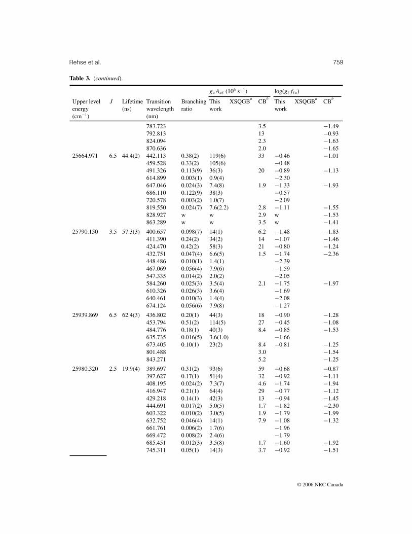
Rehse et al. 759

Table 3. (continued).

guAu� (106 s−1) log(g�f�u)

Upper levelenergy(cm−1)

J Lifetime(ns)

Transitionwavelength(nm)

Branchingratio

Thiswork

XSQGBa

CBb

Thiswork

XSQGBa

CBb

783.723 3.5 −1.49792.813 13 −0.93824.094 2.3 −1.63870.636 2.0 −1.65

25664.971 6.5 44.4(2) 442.113 0.38(2) 119(6) 33 −0.46 −1.01459.528 0.33(2) 105(6) −0.48491.326 0.113(9) 36(3) 20 −0.89 −1.13614.899 0.003(1) 0.9(4) −2.30647.046 0.024(3) 7.4(8) 1.9 −1.33 −1.93686.110 0.122(9) 38(3) −0.57720.578 0.003(2) 1.0(7) −2.09819.550 0.024(7) 7.6(2.2) 2.8 −1.11 −1.55828.927 w w 2.9 w −1.53863.289 w w 3.5 w −1.41

25790.150 3.5 57.3(3) 400.657 0.098(7) 14(1) 6.2 −1.48 −1.83411.390 0.24(2) 34(2) 14 −1.07 −1.46424.470 0.42(2) 58(3) 21 −0.80 −1.24432.751 0.047(4) 6.6(5) 1.5 −1.74 −2.36448.486 0.010(1) 1.4(1) −2.39467.069 0.056(4) 7.9(6) −1.59547.335 0.014(2) 2.0(2) −2.05584.260 0.025(3) 3.5(4) 2.1 −1.75 −1.97610.326 0.026(3) 3.6(4) −1.69640.461 0.010(3) 1.4(4) −2.08674.124 0.056(6) 7.9(8) −1.27

25939.869 6.5 62.4(3) 436.802 0.20(1) 44(3) 18 −0.90 −1.28453.794 0.51(2) 114(5) 27 −0.45 −1.08484.776 0.18(1) 40(3) 8.4 −0.85 −1.53635.735 0.016(5) 3.6(1.0) −1.66673.405 0.10(1) 23(2) 8.4 −0.81 −1.25801.488 3.0 −1.54843.271 5.2 −1.25

25980.320 2.5 19.9(4) 389.697 0.31(2) 93(6) 59 −0.68 −0.87397.627 0.17(1) 51(4) 32 −0.92 −1.11408.195 0.024(2) 7.3(7) 4.6 −1.74 −1.94416.947 0.21(1) 64(4) 29 −0.77 −1.12429.218 0.14(1) 42(3) 13 −0.94 −1.45444.691 0.017(2) 5.0(5) 1.7 −1.82 −2.30603.322 0.010(2) 3.0(5) 1.9 −1.79 −1.99632.752 0.046(4) 14(1) 7.9 −1.08 −1.32661.761 0.006(2) 1.7(6) −1.96669.472 0.008(2) 2.4(6) −1.79685.451 0.012(3) 3.5(8) 1.7 −1.60 −1.92745.311 0.05(1) 14(3) 3.7 −0.92 −1.51

© 2006 NRC Canada

760 Can. J. Phys. Vol. 84, 2006

Table 3. (continued).

guAu� (106 s−1) log(g�f�u)

Upper levelenergy(cm−1)

J Lifetime(ns)

Transitionwavelength(nm)

Branchingratio

Thiswork

XSQGBa

CBb

Thiswork

XSQGBa

CBb

26046.350 4.5 20.9(8) 434.780 0.29(2) 141(10) 42 −0.40 −0.93443.389 0.50(2) 237(14) 62 −0.15 −0.74461.544 0.14(1) 67(6) 12 −0.67 −1.42482.286 0.0035(5) 1.7(2) −2.23555.391 0.0020(3) 1.0(2) −2.35575.641 0.0024(4) 1.2(2) −2.24600.806 0.0042(5) 2.0(2) −1.97630.118 0.010(1) 4.6(5) 2.4 −1.56 −1.84723.703 0.014(1) 6.6(7) 1.9 −1.29 −1.84754.137

c0.025(2) 3.4 −1.54

757.095c

3.4 −1.54765.575 0.009(1) 4.5(6) 1.6 −1.41 −1.86

26086.631 3.5 70(2) 395.953 0.22(2) 25(2) −1.23406.431 0.20(1) 22(2) −1.26419.193 0.32(2) 36(2) −1.02442.598 0.050(5) 5.7(5) −1.78460.688 0.086(7) 9.8(9) −1.51574.309 0.009(5) 1.0(5) −2.30628.523 0.013(7) 1.5(8) −2.06692.962 0.03(1) 3.5(1.6) −1.60711.980 0.08(2) 9.2(2.4) −1.15

26159.600 3.5 93(4) 394.811 0.79(3) 68(4) 26 −0.80 −1.21405.229 0.022(5) 1.9(4) −2.34425.939 0.037(5) 3.2(5) 2.0 −2.06 −2.27441.173 0.034(5) 2.9(5) −2.07459.144 0.011(4) 0.9(4) −2.54551.918 0.010(7) 0.9(6) −2.41571.912 0.028(9) 2.4(8) −1.92689.475 0.07(3) 5.8(2.8) −1.38

26190.920 2.5 39.3(3) 386.524 0.110(8) 17(1) 12 −1.42 −1.56394.324 0.29(2) 44(3) 22 −0.99 −1.29404.715 0.33(2) 50(3) 27 −0.91 −1.18413.317 0.045(4) 6.8(6) 3.9 −1.76 −2.01425.372 0.036(3) 5.6(5) −1.82440.564 0.033(3) 5.1(5) 1.5 −1.83 −2.37595.750 0.027(5) 4.2(7) 2.4 −1.65 −1.90624.429 0.039(6) 6.0(10) −1.46652.663 0.031(8) 4.7(1.2) −1.52664.904 w w w694.624 0.06(1) 9.7(1.9) −1.15

26214.051 2.5 66(1) 386.179 0.14(1) 12.5(9) −1.55393.964 0.038(3) 3.5(3) 1.8 −2.09 −2.37404.337 0.057(5) 5.2(4) −1.90412.922 0.32(2) 29(2) 11 −1.13 −1.57424.954 0.28(2) 26(2) 8.0 −1.16 −1.67440.116 0.16(1) 15(1) −1.36

© 2006 NRC Canada

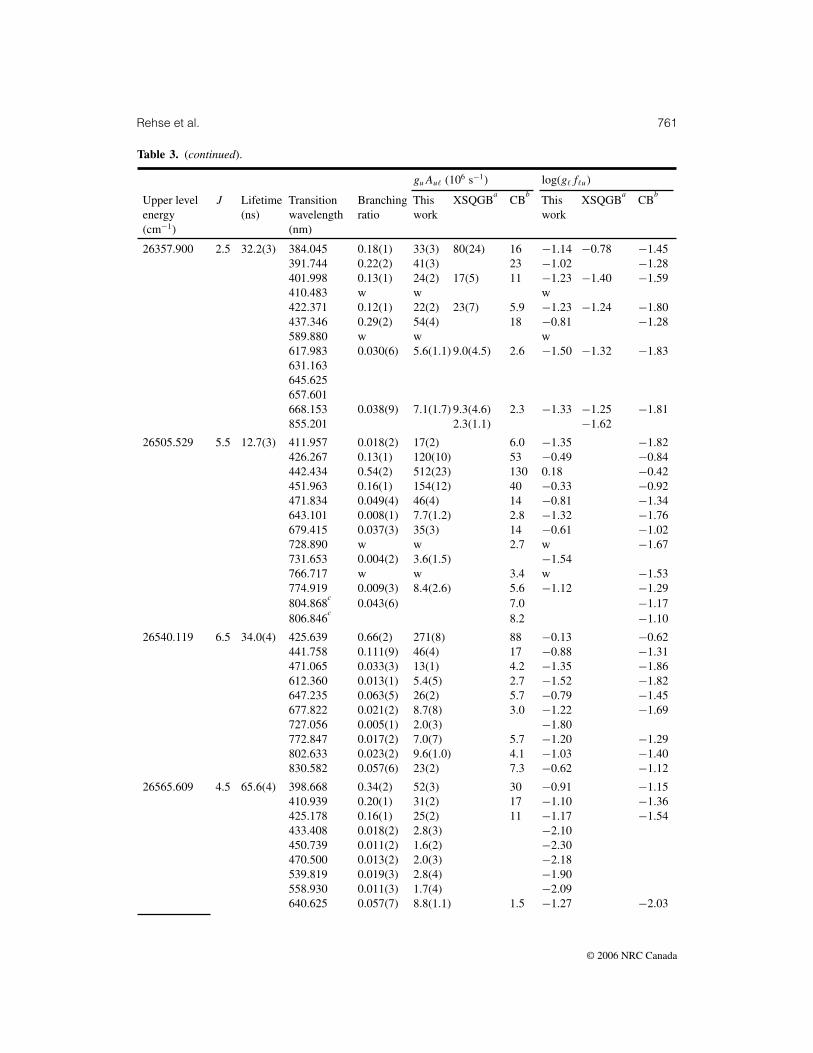
Rehse et al. 761

Table 3. (continued).

guAu� (106 s−1) log(g�f�u)

Upper levelenergy(cm−1)

J Lifetime(ns)

Transitionwavelength(nm)

Branchingratio

Thiswork

XSQGBa

CBb

Thiswork

XSQGBa

CBb

26357.900 2.5 32.2(3) 384.045 0.18(1) 33(3) 80(24) 16 −1.14 −0.78 −1.45391.744 0.22(2) 41(3) 23 −1.02 −1.28401.998 0.13(1) 24(2) 17(5) 11 −1.23 −1.40 −1.59410.483 w w w422.371 0.12(1) 22(2) 23(7) 5.9 −1.23 −1.24 −1.80437.346 0.29(2) 54(4) 18 −0.81 −1.28589.880 w w w617.983 0.030(6) 5.6(1.1) 9.0(4.5) 2.6 −1.50 −1.32 −1.83631.163645.625657.601668.153 0.038(9) 7.1(1.7) 9.3(4.6) 2.3 −1.33 −1.25 −1.81855.201 2.3(1.1) −1.62

26505.529 5.5 12.7(3) 411.957 0.018(2) 17(2) 6.0 −1.35 −1.82426.267 0.13(1) 120(10) 53 −0.49 −0.84442.434 0.54(2) 512(23) 130 0.18 −0.42451.963 0.16(1) 154(12) 40 −0.33 −0.92471.834 0.049(4) 46(4) 14 −0.81 −1.34643.101 0.008(1) 7.7(1.2) 2.8 −1.32 −1.76679.415 0.037(3) 35(3) 14 −0.61 −1.02728.890 w w 2.7 w −1.67731.653 0.004(2) 3.6(1.5) −1.54766.717 w w 3.4 w −1.53774.919 0.009(3) 8.4(2.6) 5.6 −1.12 −1.29804.868

c0.043(6) 7.0 −1.17

806.846c

8.2 −1.10

26540.119 6.5 34.0(4) 425.639 0.66(2) 271(8) 88 −0.13 −0.62441.758 0.111(9) 46(4) 17 −0.88 −1.31471.065 0.033(3) 13(1) 4.2 −1.35 −1.86612.360 0.013(1) 5.4(5) 2.7 −1.52 −1.82647.235 0.063(5) 26(2) 5.7 −0.79 −1.45677.822 0.021(2) 8.7(8) 3.0 −1.22 −1.69727.056 0.005(1) 2.0(3) −1.80772.847 0.017(2) 7.0(7) 5.7 −1.20 −1.29802.633 0.023(2) 9.6(1.0) 4.1 −1.03 −1.40830.582 0.057(6) 23(2) 7.3 −0.62 −1.12

26565.609 4.5 65.6(4) 398.668 0.34(2) 52(3) 30 −0.91 −1.15410.939 0.20(1) 31(2) 17 −1.10 −1.36425.178 0.16(1) 25(2) 11 −1.17 −1.54433.408 0.018(2) 2.8(3) −2.10450.739 0.011(2) 1.6(2) −2.30470.500 0.013(2) 2.0(3) −2.18539.819 0.019(3) 2.8(4) −1.90558.930 0.011(3) 1.7(4) −2.09640.625 0.057(7) 8.8(1.1) 1.5 −1.27 −2.03

© 2006 NRC Canada

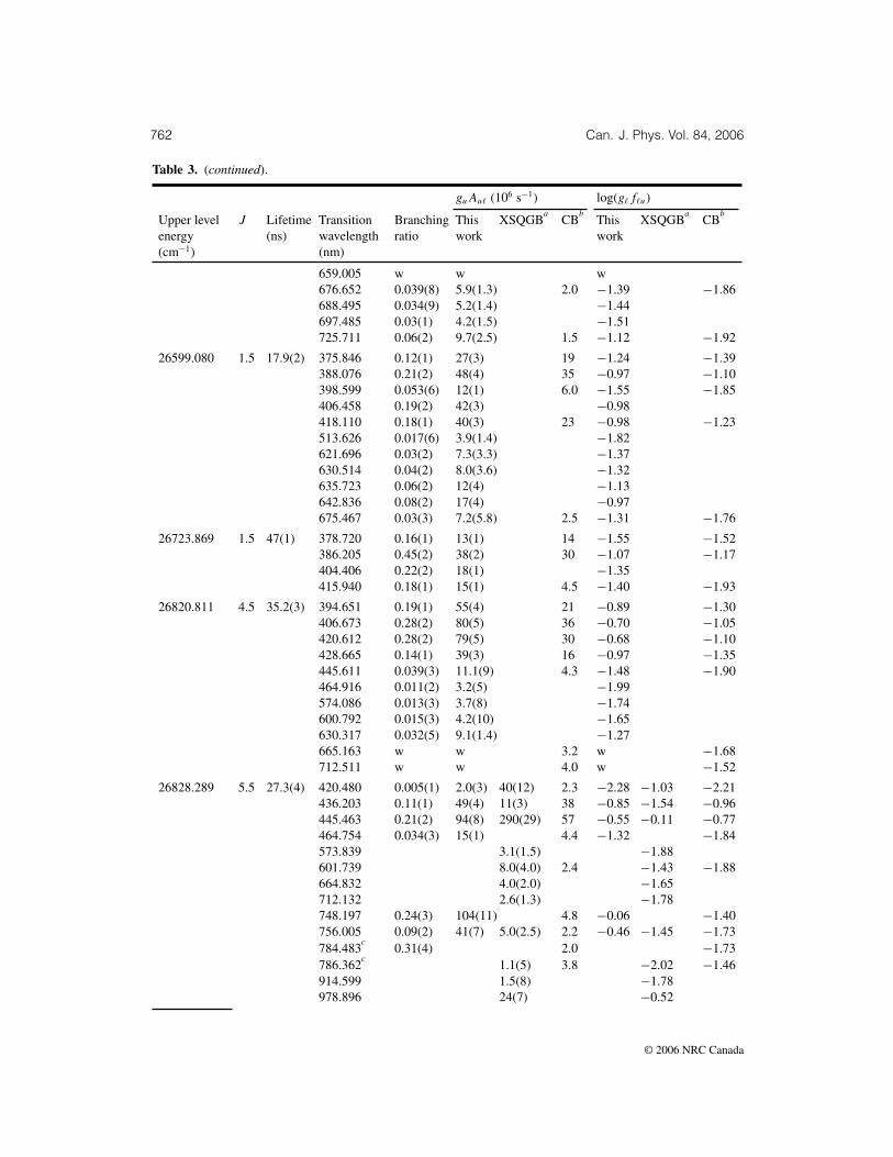
762 Can. J. Phys. Vol. 84, 2006

Table 3. (continued).

guAu� (106 s−1) log(g�f�u)

Upper levelenergy(cm−1)

J Lifetime(ns)

Transitionwavelength(nm)

Branchingratio

Thiswork

XSQGBa

CBb

Thiswork

XSQGBa

CBb

659.005 w w w676.652 0.039(8) 5.9(1.3) 2.0 −1.39 −1.86688.495 0.034(9) 5.2(1.4) −1.44697.485 0.03(1) 4.2(1.5) −1.51725.711 0.06(2) 9.7(2.5) 1.5 −1.12 −1.92

26599.080 1.5 17.9(2) 375.846 0.12(1) 27(3) 19 −1.24 −1.39388.076 0.21(2) 48(4) 35 −0.97 −1.10398.599 0.053(6) 12(1) 6.0 −1.55 −1.85406.458 0.19(2) 42(3) −0.98418.110 0.18(1) 40(3) 23 −0.98 −1.23513.626 0.017(6) 3.9(1.4) −1.82621.696 0.03(2) 7.3(3.3) −1.37630.514 0.04(2) 8.0(3.6) −1.32635.723 0.06(2) 12(4) −1.13642.836 0.08(2) 17(4) −0.97675.467 0.03(3) 7.2(5.8) 2.5 −1.31 −1.76

26723.869 1.5 47(1) 378.720 0.16(1) 13(1) 14 −1.55 −1.52386.205 0.45(2) 38(2) 30 −1.07 −1.17404.406 0.22(2) 18(1) −1.35415.940 0.18(1) 15(1) 4.5 −1.40 −1.93

26820.811 4.5 35.2(3) 394.651 0.19(1) 55(4) 21 −0.89 −1.30406.673 0.28(2) 80(5) 36 −0.70 −1.05420.612 0.28(2) 79(5) 30 −0.68 −1.10428.665 0.14(1) 39(3) 16 −0.97 −1.35445.611 0.039(3) 11.1(9) 4.3 −1.48 −1.90464.916 0.011(2) 3.2(5) −1.99574.086 0.013(3) 3.7(8) −1.74600.792 0.015(3) 4.2(10) −1.65630.317 0.032(5) 9.1(1.4) −1.27665.163 w w 3.2 w −1.68712.511 w w 4.0 w −1.52

26828.289 5.5 27.3(4) 420.480 0.005(1) 2.0(3) 40(12) 2.3 −2.28 −1.03 −2.21436.203 0.11(1) 49(4) 11(3) 38 −0.85 −1.54 −0.96445.463 0.21(2) 94(8) 290(29) 57 −0.55 −0.11 −0.77464.754 0.034(3) 15(1) 4.4 −1.32 −1.84573.839 3.1(1.5) −1.88601.739 8.0(4.0) 2.4 −1.43 −1.88664.832 4.0(2.0) −1.65712.132 2.6(1.3) −1.78748.197 0.24(3) 104(11) 4.8 −0.06 −1.40756.005 0.09(2) 41(7) 5.0(2.5) 2.2 −0.46 −1.45 −1.73784.483

c0.31(4) 2.0 −1.73

786.362c

1.1(5) 3.8 −2.02 −1.46914.599 1.5(8) −1.78978.896 24(7) −0.52

© 2006 NRC Canada

Rehse et al. 763

Table 3. (continued).

guAu� (106 s−1) log(g�f�u)

Upper levelenergy(cm−1)

J Lifetime(ns)

Transitionwavelength(nm)

Branchingratio

Thiswork

XSQGBa

CBb

Thiswork

XSQGBa

CBb

26880.600 5.5 48.4(6) 419.557 0.008(1) 2.1(2) −2.26435.210 0.35(2) 87(5) −0.61444.427 0.45(2) 112(6) −0.48463.627 0.087(7) 22(2) −1.16549.257 0.007(1) 1.7(3) −2.12572.122 0.011(1) 2.6(3) −1.89627.950 0.009(1) 2.3(3) −1.86662.527 0.009(2) 2.3(4) −1.82673.876 0.002(1) 0.6(2) −2.41712.105 0.009(2) 2.3(4) −1.76745.279 0.020(3) 4.9(7) −1.39781.276783.140 0.034(5) 8.4(1.1) −1.11

26974.670 2.5 54.4(7) 375.156 0.095(7) 10.5(8) 7.5 −1.66 −1.80382.499 0.087(7) 9.6(8) −1.68392.269 0.082(7) 9.1(7) 7.5(3.8) 3.9 −1.68 −1.79 −2.04400.344 0.24(2) 27(2) 57(17) 13 −1.19 −0.90 −1.52411.644 0.21(1) 23(2) 21(6) 8.9 −1.24 −1.30 −1.65425.855 0.29(2) 32(2) 9.3(4.7) 9.9 −1.06 −1.63 −1.57528.152 w w 3.2(1.6) w −1.92543.447 w w w658.750 w w 0.2(1) w −1.85812.342 1.4(7) −1.88

27107.619 3.5 41.4(2) 380.563 0.13(1) 25(2) 16 −1.26 −1.47390.233 0.025(5) 4.9(9) 3.4 −1.95 −2.11401.983 0.070(7) 14(1) 5.6 −1.48 −1.87409.403 0.16(1) 31(2) 14 −1.11 −1.45423.457 0.49(2) 94(4) 31 −0.60 −1.08439.987 0.060(7) 12(1) 4.6 −1.47 −1.88542.491 0.012(3) 2.4(6) −1.97619.122 0.018(6) 3.4(1.1) −1.71663.721 0.04(1) 6.8(1.9) −1.35687.529 w w 1.7 w −1.93

27165.350 2.5 64(3) 372.490 0.30(2) 28(2) 20(6) 21 −1.24 −1.45 −1.36379.729 0.20(2) 19(2) 21 −1.38 −1.34389.356397.310 0.049(7) 4.6(7) −1.96408.437 0.21(2) 20(2) 9.1(4.6) 11 −1.31 −1.70 −1.57422.424 0.075(8) 7.1(8) 2.6 −1.72 −2.16509.010 0.048(7) 4.5(7) −1.75522.885 0.10(1) 9.3(1.1) −1.42537.871 0.017(6) 1.6(5) −2.15799.947 1.5(8) −1.92

© 2006 NRC Canada

764 Can. J. Phys. Vol. 84, 2006

Table 3. (continued).

guAu� (106 s−1) log(g�f�u)

Upper levelenergy(cm−1)

J Lifetime(ns)

Transitionwavelength(nm)

Branchingratio

Thiswork

XSQGBa

CBb

Thiswork

XSQGBa

CBb

27188.301 3.5 26.9(4) 379.398 0.32(8) 95(23) 80 −0.69 −0.76389.008 0.16(5) 46(15) 32 −0.98 −1.14400.683 0.02(1) 7.1(3.0) 4.2 −1.77 −1.99408.055 0.09(3) 25(9) 12 −1.20 −1.54422.015 0.08(3) 23(8) 8.9 −1.20 −1.62438.430 0.10(4) 30(11) 15 −1.06 −1.35540.126 0.010(6) 3.0(1.7) −1.89587.810 0.02(1) 5.9(3.3) 1.9 −1.52 −2.01616.043 0.04(3) 12(8) 3.3 −1.17 −1.73633.021 0.02(2) 7.1(5.6) −1.37660.183 0.10(5) 30(13) 7.0 −0.71 −1.34668.445 0.04(3) 12(9) −1.08

27263.250 7.5 29.2(2) 428.079 0.80(2) 437(9) 120 0.08 −0.50618.289 0.015(1) 8.2(8) 4.5 −1.33 −1.59656.929 0.15(1) 81(7) 24 −0.28 −0.81758.591 0.010(1) 5.5(6) 6.8 −1.32 −1.23783.509 0.029(3) 16(2) 8.5 −0.83 −1.11

27284.689 2.5 17.3(2) 370.841 0.14(1) 48(4) 35(10) 24 −1.01 −1.19 −1.30378.015 0.013(2) 4.5(5) −2.01387.554 0.14(1) 47(3) 30 −0.98 −1.18406.455 0.24(2) 84(5) 145(15) 70 −0.68 −0.49 −0.76420.305 0.32(2) 113(6) 104(10) 57 −0.53 −0.61 −0.82519.642 0.006(2) 2.1(5) 2.9(1.4) −2.07 −1.99615.692 0.016(3) 5.5(1.2) 3.6(1.8) −1.50 −1.72619.815 0.021(4) 7.2(1.3) −1.38629.181 0.031(4) 11(1) 2.4(1.2) 8.0 −1.20 −1.92 −1.32639.828 0.021(4) 7.3(1.5) −1.35645.562 0.028(5) 9.6(1.6) 12(4) 2.3 −1.22 −1.15 −1.83679.258 0.027(6) 9.4(2.1) 2.5 −1.19 −1.77699.263 2.2(1.1) −1.80792.380 2.0(1.0) −1.78

892.059 1.3(6) −1.87972.534 3.4(1.7) −1.36

27309.730 4.5 38(2) 387.178 0.23(2) 61(5) 42 −0.87 −1.02398.742 0.113(9) 30(3) 18 −1.15 −1.36412.135 0.18(1) 46(4) 21 −0.93 −1.27436.107 0.13(1) 34(3) 12 −1.01 −1.47454.580 0.030(3) 7.9(9) 1.7 −1.61 −2.29583.643 0.037(8) 9.6(2.1) −1.31611.468 0.05(1) 14(3) 2.8 −1.11 −1.81663.062 0.04(1) 11(4) 2.4 −1.12 −1.80688.519 0.19(2) 5.0 −1.45690.984 2.5 −1.74

© 2006 NRC Canada

Rehse et al. 765

Table 3. (continued).

guAu� (106 s−1) log(g�f�u)

Upper levelenergy(cm−1)

J Lifetime(ns)

Transitionwavelength(nm)

Branchingratio

Thiswork

XSQGBa

CBb

Thiswork

XSQGBa

CBb

27464.199 3.5 36.9(8) 375.466 0.017(2) 3.8(5) −2.10384.876 0.056(5) 12(1) 27(8) −1.57 −1.24396.301 0.33(2) 70(4) −0.78403.510 0.31(2) 67(4) 26(8) 39 −0.79 −1.21 −1.03417.156 0.19(1) 41(3) 8.6(4.3) 22 −0.97 −1.66 −1.24433.189 0.010(1) 2.1(3) −2.22532.193 0.010(2) 2.2(4) −2.04553.734 0.006(2) 1.4(4) −2.21578.426 6.7(3.3) −1.49602.573 4.5(2.2) −1.63605.745 5.3(2.7) −1.55622.152 6.1(3.0) −1.47632.560 0.035(5) 7.5(1.1) 0.5(2) −1.35 −1.58648.370 0.016(4) 3.5(9) 12(4) −1.66 −1.15656.337 0.029(5) 6.3(1.2) 3.3(1.7) −1.39 −1.69671.073 w w w818.022 1.7(8) −1.76

27695.961 6.5 24.6(5) 420.291 0.067(6) 38(4) 67(20) 38 −1.00 −0.80 −1.00446.734 0.902(9) 513(12) 592(59) 140 0.19 0.19 −0.39602.174 0.006(2) 3.4(9) −1.73628.563702.574734.475757.810 0.025(4) 14(3) 17(5) 4.6 −0.90 −0.94 −1.40902.242 1.8(9) −1.73970.224 46(14) −0.28

28072.330 3.5 9.96(9) 367.082 0.31(2) 248(14) 150 −0.30 −0.52376.071 0.20(1) 163(11) 120 −0.46 −0.60393.843 w w 1.8 w −2.38406.832 0.107(8) 86(6) 44 −0.67 −0.96422.066 0.22(1) 176(11) 48 −0.33 −0.89

486.539499.203 0.037(4) 30(3) 11 −0.95 −1.37515.504 0.104(9) 83(7) 58 −0.48 −0.63581.266599.465 0.022(6) 18(5) 4.8 −1.02 −1.59623.766 5.7 −1.48644.753699.340

28151.400 5.5 29.3(4) 385.791 0.10(1) 42(4) 32 −1.03 −1.14398.314 0.24(2) 97(7) 46 −0.64 −0.96412.395 0.20(2) 82(6) 46 −0.68 −0.93420.662 0.14(1) 59(5) 18 −0.81 −1.33437.824 0.23(2) 93(7) 61 −0.57 −0.76611.065 0.044(6) 18(2) 8.5 −1.00 −1.32687.242 0.05(1) 18(4) 6.4 −0.89 −1.35712.237 w w 3.0 w −1.65

© 2006 NRC Canada

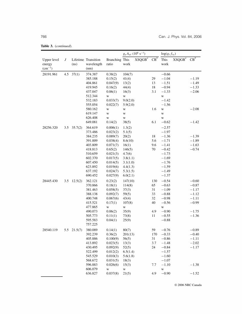
766 Can. J. Phys. Vol. 84, 2006

Table 3. (continued).

guAu� (106 s−1) log(g�f�u)

Upper levelenergy(cm−1)

J Lifetime(ns)

Transitionwavelength(nm)

Branchingratio

Thiswork

XSQGBa

CBb

Thiswork

XSQGBa

CBb

28191.961 4.5 37(1) 374.387 0.38(2) 104(7) −0.66385.188 0.15(2) 41(4) 29 −1.04 −1.19404.861 0.047(9) 13(2) 13 −1.51 −1.49419.945 0.16(2) 44(4) 18 −0.94 −1.33437.047 0.06(1) 16(3) 3.1 −1.33 −2.06512.344 w w w532.183 0.033(7) 9.0(2.0) −1.42555.054 0.022(7) 5.9(2.0) −1.56580.162 w w 1.6 w −2.08619.147 w w w626.408 w w w649.081 0.14(2) 38(5) 6.1 −0.62 −1.42

28256.320 3.5 35.7(2) 364.619 0.006(1) 1.3(2) −2.57373.486 0.023(2) 5.1(5) −1.97384.235 0.089(7) 20(2) 18 −1.36 −1.39391.009 0.038(4) 8.6(10) 5.6 −1.71 −1.89403.809 0.071(7) 16(1) 9.6 −1.41 −1.63418.813 0.65(2) 146(5) 70 −0.42 −0.74510.659 0.021(3) 4.7(6) −1.73602.370 0.017(5) 3.8(1.1) −1.69607.450 0.014(5) 3.1(1.0) −1.76623.892 0.019(6) 4.4(1.3) −1.59637.192 0.024(7) 5.3(1.5) −1.49690.452 0.027(9) 6.0(2.1) −1.37

28445.430 3.5 12.5(2) 362.121 0.23(2) 147(10) 130 −0.54 −0.60370.866 0.18(1) 114(8) 65 −0.63 −0.87381.463 0.058(5) 37(3) 31 −1.09 −1.17388.138 0.092(7) 59(5) 33 −0.88 −1.12400.748 0.067(6) 43(4) 32 −0.98 −1.11415.521 0.17(1) 107(8) 40 −0.56 −0.99477.865 w w w490.073 0.06(2) 35(9) 4.9 −0.90 −1.75505.773 0.11(1) 73(8) 11 −0.55 −1.36595.583 0.04(1) 25(9) −0.88757.225

28540.119 5.5 21.5(7) 380.089 0.14(1) 80(7) 59 −0.76 −0.89392.239 0.36(2) 201(13) 170 −0.33 −0.40405.886 0.100(9) 56(5) 31 −0.86 −1.11413.892 0.023(5) 13(3) 3.7 −1.48 −2.02430.495 0.092(9) 52(5) 24 −0.84 −1.17522.499 0.012(2) 6.5(1.4) −1.57545.529 0.010(3) 5.6(1.8) −1.60568.672 0.031(5) 18(3) −1.07596.883 0.026(6) 15(3) 7.7 −1.10 −1.38606.079 w w w636.827 0.037(8) 21(5) 4.9 −0.90 −1.52

© 2006 NRC Canada

Rehse et al. 767

Table 3. (concluded).

guAu� (106 s−1) log(g�f�u)

Upper levelenergy(cm−1)

J Lifetime(ns)

Transitionwavelength(nm)

Branchingratio

Thiswork

XSQGBa

CBb

Thiswork

XSQGBa

CBb

663.228 0.08(1) 43(6) −0.54669.356 0.09(1) 48(7) 17 −0.49 −0.93

28725.529 4.5 38.1(2) 367.052 0.034(3) 8.8(9) −1.75377.429 0.029(3) 7.7(8) 23 −1.79 −1.32389.406 0.14(1) 37(3) 32 −1.07 −1.14396.298 0.15(1) 39(3) −1.04410.739 0.43(2) 113(5) −0.54427.085 0.22(2) 57(4) 12 −0.81 −1.50498.707 w w w517.484 w w w562.737 w w w576.870 w w w627.348 w w w668.780 w w w

28913.990 4.5 14.9(1) 364.529 0.097(7) 65(5) 31 −0.89 −1.20374.762 0.093(7) 62(5) 39 −0.88 −1.09386.568 0.014(1) 9.5(10) 6.7 −1.67 −1.83393.359 0.068(5) 46(3) −0.98407.583 0.24(2) 162(10) 64 −0.40 −0.79423.674 0.39(2) 262(13) 97 −0.15 −0.58494.062 0.019(2) 13(1) −1.34512.484 0.030(3) 20(2) −1.09660.453 0.047(7) 32(5) −0.68

28997.141 4.5 9.6(5) 363.427 0.52(3) 542(40) 300 0.03 −0.23373.597 0.26(2) 269(25) 130 −0.25 −0.56385.329 0.03(1) 31(13) −1.16422.186 0.017(4) 17(4) −1.33477.168 w w w492.039 0.030(9) 32(10) 12 −0.94 −1.38510.309 0.11(3) 112(27) 54 −0.36 −0.68589.739

c0.025(8) 10 −1.27

596.323c

6.1 −1.48616.834 0.011(4) 12(4) 2.9 −1.18 −1.78763.177

29387.869 4.5 59(1) 358.337 0.17(2) 29(4) 31 −1.25 −1.23368.221 0.06(2) 10(3) −1.67386.159 0.05(2) 9.2(2.9) −1.69415.333 0.63(3) 106(6) 49 −0.56 −0.90482.756 0.023(5) 3.9(8) −1.86640.404 0.06(2) 11(2) −1.18

aRef. 14.bRef. 8.cUnresolved lines in this work.

© 2006 NRC Canada

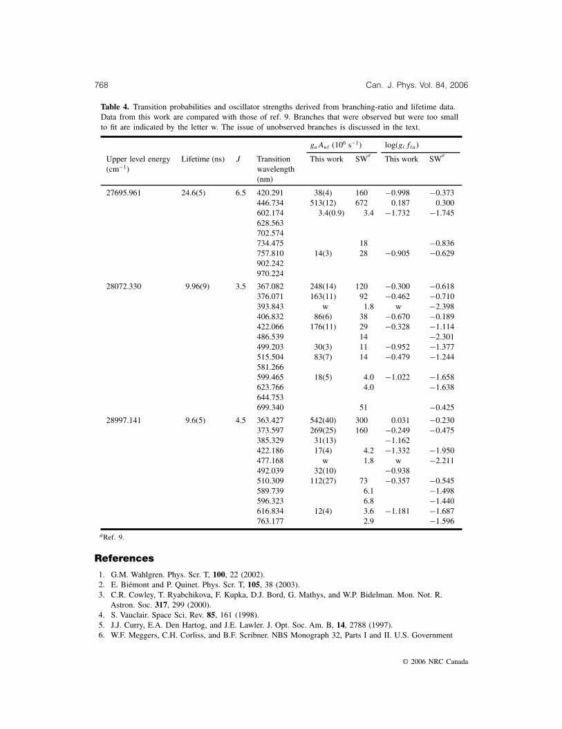
768 Can. J. Phys. Vol. 84, 2006

Table 4. Transition probabilities and oscillator strengths derived from branching-ratio and lifetime data.Data from this work are compared with those of ref. 9. Branches that were observed but were too smallto fit are indicated by the letter w. The issue of unobserved branches is discussed in the text.

guAu� (106 s−1) log(g�f�u)

Upper level energy(cm−1)

Lifetime (ns) J Transitionwavelength(nm)

This work SWa

This work SWa

27695.961 24.6(5) 6.5 420.291 38(4) 160 −0.998 −0.373446.734 513(12) 672 0.187 0.300602.174 3.4(0.9) 3.4 −1.732 −1.745628.563702.574734.475 18 −0.836757.810 14(3) 28 −0.905 −0.629902.242970.224

28072.330 9.96(9) 3.5 367.082 248(14) 120 −0.300 −0.618376.071 163(11) 92 −0.462 −0.710393.843 w 1.8 w −2.398406.832 86(6) 38 −0.670 −0.189422.066 176(11) 29 −0.328 −1.114486.539 14 −2.301499.203 30(3) 11 −0.952 −1.377515.504 83(7) 14 −0.479 −1.244581.266599.465 18(5) 4.0 −1.022 −1.658623.766 4.0 −1.638644.753699.340 51 −0.425

28997.141 9.6(5) 4.5 363.427 542(40) 300 0.031 −0.230373.597 269(25) 160 −0.249 −0.475385.329 31(13) −1.162422.186 17(4) 4.2 −1.332 −1.950477.168 w 1.8 w −2.211492.039 32(10) −0.938510.309 112(27) 73 −0.357 −0.545589.739 6.1 −1.498596.323 6.8 −1.440616.834 12(4) 3.6 −1.181 −1.687763.177 2.9 −1.596

aRef. 9.

References

1. G.M. Wahlgren. Phys. Scr. T, 100, 22 (2002).2. E. Biémont and P. Quinet. Phys. Scr. T, 105, 38 (2003).3. C.R. Cowley, T. Ryabchikova, F. Kupka, D.J. Bord, G. Mathys, and W.P. Bidelman. Mon. Not. R.

Astron. Soc. 317, 299 (2000).4. S. Vauclair. Space Sci. Rev. 85, 161 (1998).5. J.J. Curry, E.A. Den Hartog, and J.E. Lawler. J. Opt. Soc. Am. B, 14, 2788 (1997).6. W.F. Meggers, C.H. Corliss, and B.F. Scribner. NBS Monograph 32, Parts I and II. U.S. Government

© 2006 NRC Canada

Rehse et al. 769

Printing Office, Washington, DC. 1961.7. W.F. Meggers, C.H. Corliss, and B.F. Scribner. NBS Monograph 145, Parts I and II. U.S. Government

Printing Office, Washington, DC. 1975.8. C.H. Corliss and W.R. Bozman. Monograph 53. U.S. National Bureau of Standards, Washington, DC.9. L. Saffman and W. Whaling. J. Quantum. Spectrosc. Radiat. Trans. 21, 93 (1979).

10. T. Andersen, O. Poulsen, T.S. Ramanujam, and A.P. Petkov. Sol. Phys. 44, 257 (1975).11. R.L. Kurucz and B. Bell. Atomic line data. Kurucz CD-ROM No. 23. Smithsonian Astrophysical

Observatory, Cambridge, Mass. 1995.12. http://cfa-www.harvard.edu/amdata/ampdata/kurucz23/sekur.html13. A. Kastberg, P. Villemoes, A. Arnesen, F. Heijkenskjöld, A. Langereis, P. Jungner, and S. Linnæus. Z.

Phys. D, 28, 289 (1993).14. H.L. Xu, S. Svanberg, P. Quinet, H.P. Garnir, and E. Biémont. J. Phys. B: At. Mol. Phys. 36, 4773

(2003).15. http://w3.umh.ac.be/∼astro/dream.shtml16. T.J. Scholl, R.A. Holt, D. Masterman, R.C. Rivest, S.D. Rosner, and A. Sharikova. Can. J. Phys. 80,

1621 (2002).17. Z. Zhiguo, Z.S. Li, H. Lundberg, K.Y. Zhang, Z.W. Dai, J. Zhankui, and S. Svanberg. J. Phys. B: At.

Mol. Opt. Phys. 33, 521 (2000).18. W. Demtröder. Laser spectroscopy. Springer, Berlin. 1996.19. S.L. Kaufman. Opt. Commun. 17, 309 (1976).20. J.L. Hall and S.A. Lee. Appl. Phys. Lett. 29, 367 (1976).21. L.H. Cadwell. Am. J. Phys. 64, 917 (1996).22. P.M. Kock, L.D. Gardner, and J.E. Bayfield. In Beam-foil spectroscopy. Vol. 2. Edited by I.A. Sellin and

D.J. Pegg. Plenum, New York. 1976. p. 829.23. L. Kay and R. Shepherd. J. Phys. E: Sci. Instrum. 16, 295 (1983).24. W.C. Martin and W.L. Wiese. In Atomic, molecular, & optical physics handbook. Edited by G.W.F.

Drake. AIP, New York. 1996.

Appendix A. Fiber array design

In this experiment it is very important that the observed LIF intensities be accurately proportionalto the Einstein A coefficients for spontaneous emission. Excitation of ions by a linearly polarized laserbeam produces unequal populations in the Zeeman sublevels of the upper state, characterized as analignment, resulting in an anisotropic radiation pattern. The practical impossibility of constructing animpartial 4π -solid-angle LIF detector introduces a potential bias into branching-ratio measurements. Inthis Appendix, we show that this source of systematic error can be eliminated by careful design of thedetection system, and present two different solutions to the problem, both of which were implementedin our apparatus.

Consider a transition from a given upper leveluwith angular-momentum quantum numbersJu, Mu =Ju, Ju − 1, . . . ,−Ju to a given lower level � with corresponding quantum numbers J�, M� = J�, J� −1, . . . ,−J�. We take the z-axis along the direction of the electric field of the laser radiation. The upper-level populations P(Mu) created by absorption of laser photons will be unequal, and are assumed to becompletely arbitrary. The electric-dipole selection rules allow a given sublevel Mu to decay to (at most)three lower levels, M� = Mu + �M where �M = 0, ±1, with relative probabilities given [A.1]by thesquared Clebsch–Gordan coefficients |〈Ju, Mu, 1, �M | J�, M�〉|2. These three �M = 0, ±1 transi-tions have electric-dipole angular distributions [A.1] given by

S�M(θ) ={( 3

8π

)sin2 θ, �M = 0( 3

8π

) 12

(1 + cos2 θ

), �M = ±1

(A1)

The total rate of spontaneous emission from a particular sublevel Mu via the branch u → � is givenby the product P (Mu) Au�. To calculate the rate of emission into the solid angle sin θ dθ dφ, we

© 2006 NRC Canada

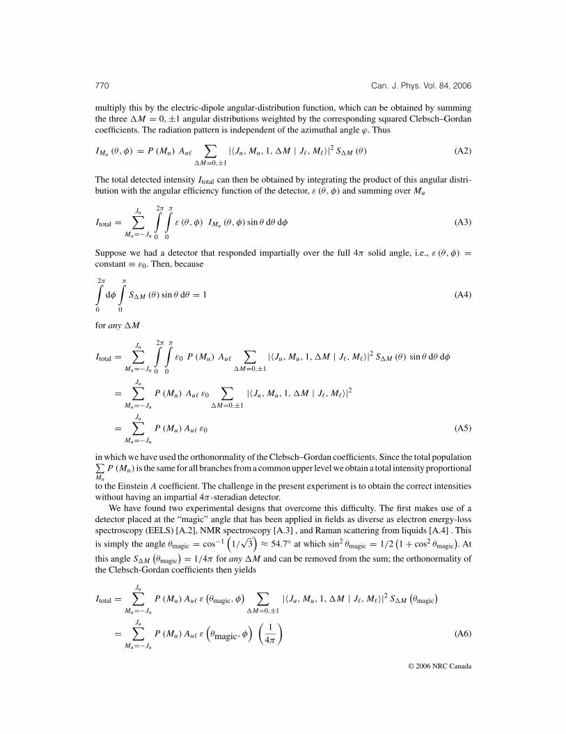
770 Can. J. Phys. Vol. 84, 2006

multiply this by the electric-dipole angular-distribution function, which can be obtained by summingthe three �M = 0, ±1 angular distributions weighted by the corresponding squared Clebsch–Gordancoefficients. The radiation pattern is independent of the azimuthal angle ϕ. Thus

IMu (θ, φ) = P (Mu) Au�

∑�M=0,±1

|〈Ju, Mu, 1, �M | J�, M�〉|2 S�M (θ) (A2)

The total detected intensity Itotal can then be obtained by integrating the product of this angular distri-bution with the angular efficiency function of the detector, ε (θ, φ) and summing over Mu

Itotal =Ju∑

Mu=−Ju

2π∫0

π∫0

ε (θ, φ) IMu (θ, φ) sin θ dθ dφ (A3)

Suppose we had a detector that responded impartially over the full 4π solid angle, i.e., ε (θ, φ) =constant ≡ ε0. Then, because

2π∫0

dφ

π∫0

S�M (θ) sin θ dθ = 1 (A4)

for any �M

Itotal =Ju∑

Mu=−Ju

2π∫0

π∫0

ε0 P (Mu) Au�

∑�M=0,±1

|〈Ju, Mu, 1, �M | J�, M�〉|2 S�M (θ) sin θ dθ dφ

=Ju∑

Mu=−Ju

P (Mu) Au� ε0

∑�M=0,±1

|〈Ju, Mu, 1, �M | J�, M�〉|2

=Ju∑

Mu=−Ju

P (Mu) Au� ε0 (A5)

in which we have used the orthonormality of the Clebsch–Gordan coefficients. Since the total population∑Mu

P (Mu) is the same for all branches from a common upper level we obtain a total intensity proportional

to the Einstein A coefficient. The challenge in the present experiment is to obtain the correct intensitieswithout having an impartial 4π -steradian detector.

We have found two experimental designs that overcome this difficulty. The first makes use of adetector placed at the “magic” angle that has been applied in fields as diverse as electron energy-lossspectroscopy (EELS) [A.2], NMR spectroscopy [A.3] , and Raman scattering from liquids [A.4] . This

is simply the angle θmagic = cos−1(

1/√

3)

≈ 54.7◦ at which sin2 θmagic = 1/2(1 + cos2 θmagic

). At

this angle S�M

(θmagic

) = 1/4π for any �M and can be removed from the sum; the orthonormality ofthe Clebsch-Gordan coefficients then yields

Itotal =Ju∑

Mu=−Ju

P (Mu) Au� ε(θmagic, φ

) ∑�M=0,±1

|〈Ju, Mu, 1, �M | J�, M�〉|2 S�M

(θmagic

)

=Ju∑

Mu=−Ju

P (Mu) Au� ε(θmagic, φ

) (1

4π

)(A6)

© 2006 NRC Canada

Rehse et al. 771

and is thus proportional to the Einstein A coefficient. In our LIF detector, one set of fibers is arrangedat polar angles close to θmagic.

A second solution to the problem is suggested by the solid-angle integration in (A.4). If we were tosimply arrange a ring of fibers uniformly distributed in θ , we would have an approximate experimentalrealization of the integral

∫dθ ; however, if instead we dispose the fibers non-uniformly in such a manner

as to have a density of fibers dN/dθ ∝ sin θ , the collected signal from a single ring of fibers will ineffect perform the correct 4π solid-angle integration

∫dθ sin θ “in hardware”.

Numerical studies of both of these techniques verified that neither employment of a finite acceptanceangle centred at the magic angle nor the finite approximation to the sin θ density distribution had anappreciable effect on obtaining accurate BRs. As a further check, we interchanged the roles of the twosets of fibers in the experiment and found no significant change in the measured BRs, as discussedabove.

References

A.1. E.U. Condon and G.H. Shortley. The theory of atomic spectra. Cambridge University Press,London, 1967. Chap. 4, Sect. 5.A.2. Y. Sun and J. Yuan. Phys. Rev. B, 71, 125109-1 (2005).A.3. I.J. Lowe. Phys. Rev. Lett. 2, 285 (1959).A.4. L.J. Kaufman, J. Heo, L.D. Ziegler, and G.R. Fleming. Phys. Rev. Lett. 88, 207402-1 (2002).

© 2006 NRC Canada