fast large-sample goodness-of-fit tests for copulas - Institute of

Statistica Sinica 21 (2011), 841-871

FAST LARGE-SAMPLE GOODNESS-OF-FIT TESTS

FOR COPULAS

Ivan Kojadinovic, Jun Yan and Mark Holmes

Universite de Pau et des Pays de l’Adour, University of Connecticutand The University of Auckland

Abstract: Goodness-of-fit tests are a fundamental element in the copula-based mod-

eling of multivariate continuous distributions. Among the different procedures pro-

posed in the literature, recent large scale simulations suggest that one of the most

powerful tests is based on the empirical process comparing the empirical copula

with a parametric estimate of the copula derived under the null hypothesis. As

for most of the currently available goodness-of-fit procedures for copula models,

the null distribution of the statistic for the latter test is obtained by means of a

parametric bootstrap. The main inconvenience of this approach is its high compu-

tational cost, which, as the sample size increases, can be regarded as an obstacle to

its application. In this work, fast large-sample tests for assessing goodness of fit are

obtained by means of multiplier central limit theorems. The resulting procedures

are shown to be asymptotically valid when based on popular method-of-moment

estimators. Large scale Monte Carlo experiments, involving six frequently used

parametric copula families and three different estimators of the copula parameter,

confirm that the proposed procedures provide a valid, much faster alternative to

the corresponding parametric bootstrap-based tests. An application of the derived

tests to the modeling of a well-known insurance data set is presented. The use of the

multiplier approach instead of the parametric bootstrap can reduce the computing

time from about a day to minutes.

Key words and phrases: Empirical process, multiplier central limit theorem, pseudo-

observation, rank, semiparametric model.

1. Introduction

The copula-based modeling of multivariate distributions is finding extensiveapplications in fields such as finance (Cherubini, Vecchiato, and Luciano (2004)),(McNeil, Frey, and Embrechts (2005)), hydrology (Salvadori et al. (2007)), publichealth (Cui and Sun (2004)), and actuarial sciences (Frees and Valdez (1998)).The recent enthusiasm for the use of this modeling approach finds its origin inan elegant representation theorem due to Sklar (1959) that we present here inthe bivariate case. Let (X,Y ) be a random vector with continuous marginal

842 IVAN KOJADINOVIC, JUN YAN AND MARK HOLMES

cumulative distribution functions (c.d.f.s) F and G. A consequence of the workof Sklar (1959) is that the c.d.f. H of (X,Y ) can be uniquely represented as

H(x, y) = C{F (x), G(y)}, x, y ∈ R,

where C : [0, 1]2 → [0, 1], called a copula, is a bivariate c.d.f. with standarduniform margins. Given a random sample (X1, Y1), . . . , (Xn, Yn) from c.d.f. H,this representation suggests breaking the multivariate model building into twoindependent parts: the fitting of the marginal c.d.f.s and the calibration of anappropriate parametric copula. The problem of estimating the parameters of thechosen copula has been extensively studied in the literature (see e.g., Genest,Ghoudi, and Rivest (1995), Shih and Louis (1995), Joe (1997), Genest and Favre(2007)). Another very important issue that is currently drawing a lot of attentionis whether the unknown copula C actually belongs to the chosen parametriccopula family or not. More formally, one wants to test

H0 : C ∈ C = {Cθ : θ ∈ O} against H1 : C 6∈ C,

where O is an open subset of Rq for some integer q ≥ 1.A relatively large number of testing procedures have been proposed in the

literature, as can be concluded from the recent review of Genest, Remillard, andBeaudoin (2009). Among the existing procedures, these authors advocate the useof so-called “blanket tests”, i.e., those whose implementation requires neither anarbitrary categorization of the data, nor any strategic choice of smoothing param-eter, weight function, kernel, window, etc. Among the tests in this last category,one approach that appears to perform particularly well according to recent largescale simulations (Genest, Remillard, and Beaudoin (2009), Berg (2009)) is basedon the empirical copula (Deheuvels (1981)) of the data (X1, Y1), . . . , (Xn, Yn), de-fined as

Cn(u, v) =1n

n∑i=1

1(Ui,n ≤ u, Vi,n ≤ v), u, v ∈ [0, 1], (1.1)

where the random vectors (Ui,n, Vi,n) are pseudo-observations from C computedfrom the data by

Ui,n =1

n + 1

n∑j=1

1(Xj ≤ Xi), Vi,n =1

n + 1

n∑j=1

1(Yj ≤ Yi), i∈{1, . . . , n}.

The empirical copula Cn is a consistent estimator of the unknown copulaC, whether H0 is true or not. Hence, as suggested in Fermanian (2005), Quessy(2005), and Genest and Remillard (2008), a natural goodness-of-fit test consists

FAST LARGE-SAMPLE GOODNESS-OF-FIT TESTS FOR COPULAS 843

of comparing Cn with an estimation Cθn of C obtained assuming that C ∈ Cholds. Here, θn is an estimator of θ computed from the pseudo-observations(U1,n, V1,n), . . . , (Un,n, Vn,n). More precisely, these authors propose to base a testof goodness of fit on the empirical process

√n{Cn(u, v) − Cθn(u, v)}, u, v ∈ [0, 1]. (1.2)

According to the large scale simulations carried out in Genest, Remillard, andBeaudoin (2009), the most powerful version of this procedure is based on theCramer-von Mises statistic

Sn =∫

[0,1]2n{Cn(u, v) − Cθn(u, v)}2dCn(u, v)

=n∑

i=1

{Cn(Ui,n, Vi,n) − Cθn(Ui,n, Vi,n)}2.

An approximate p-value for the test based on the above statistic is obtainedby means of a parametric bootstrap whose validity was recently shown by Gen-est and Remillard (2008). The large scale simulations carried out by Genest,Remillard, and Beaudoin (2009) and Berg (2009) suggest that, overall, this pro-cedure yields the most powerful blanket goodness-of-fit test for copula models.The main inconvenience of this approach is its high computational cost as eachparametric bootstrap iteration requires both random number generation fromthe fitted copula and estimation of the copula parameter. To fix ideas, Genest,Remillard, and Beaudoin (2009) mention the nearly exclusive use of 140 CPUsover a one-month period to estimate approximately 2000 powers and levels ofgoodness-of-fit tests based on parametric bootstrapping for n ∈ {50, 150}.

As the sample size increases, the application of parametric bootstrap-basedgoodness-of-fit tests becomes prohibitive. In order to circumvent this very highcomputational cost, we propose a fast large-sample testing procedure based onmultiplier central limit theorems. Such techniques have already been used tosimulate the null distributions of statistics in other types of tests based on em-pirical processes; see e.g., Lin, Fleming, and Wei (1994) and Fine, Yan, andKosorok (2004) for applications in survival analysis or, more recently, Scaillet(2005), and Remillard and Scaillet (2009) for applications in the copula model-ing context. Starting from the seminal work of Remillard and Scaillet (2009), wegive two multiplier central limit theorems that suggest a fast asymptotically validgoodness-of-fit procedure. As we shall see in Section 5, for n ≈ 1,500, some com-putations that would typically require about a day when based on a parametricbootstrap can be performed in minutes when based on the multiplier approach.

The second section of the paper is devoted to the asymptotic behaviorof the goodness-of-fit process

√n(Cn−Cθn) under the null hypothesis, and to


a brief presentation of the three most frequently used rank-based estimatorsof θ. In Section 3, we give two multiplier central limit theorems that are atthe root of the proposed fast asymptotically valid goodness-of-fit procedures.Section 4 discusses extensive simulation results for n = 75, 150 and 300, andfor three different rank-based estimators of the parameter θ. For n = 150, theresulting estimated powers and levels are compared with those obtained inGenest, Remillard, and Beaudoin (2009) using a parametric bootstrap. Theproofs of the theorems and the details of the computations are relegated to theappendices. The penultimate section is devoted to an application of the proposedprocedures to the modeling of dependence in well-known insurance data, while thelast section contains methodological recommendations and concluding remarks.

Finally, note that all the tests studied in this work are implemented in thecopula R package (Yan and Kojadinovic (2010)) available on the ComprehensiveR Archive Network (R Development Core Team (2009)).

2. Asymptotic Behavior of the Goodness-of-fit Process

In order to simplify the forthcoming expositions, we restrict our attention tobivariate one-parameter families of copulas, although many of the derivations tofollow can be extended to the multivariate multiparameter case at the expenseof higher complexity. Thus, let O be an open subset of R, let C = {Cθ : θ ∈ O}be an identifiable family of copulas, and assume that the true unknown copulabelongs to the family C, i.e., there exists a unique θ ∈ O such that C = Cθ.

The weak limit of the goodness-of-fit process (1.2) under the previous hy-potheses partly follows from an important result that characterizes the asymp-totic behavior of the empirical copula (see e.g., Ganssler and Stute (1987), Fer-manian, Radulovic, and Wegkamp (2004), Tsukahara (2005)).

Theorem 1. Suppose that Cθ has continuous partial derivatives. Then the em-pirical copula process

√n(Cn − Cθ) converges weakly in `∞([0, 1]2) to the tight

centered Gaussian process

Cθ(u, v) = αθ(u, v) − C[1]θ (u, v)αθ(u, 1) − C

[2]θ (u, v)αθ(1, v), u, v ∈ [0, 1],

where C[1]θ = ∂Cθ/∂u, C

[2]θ = ∂Cθ/∂v, and αθ is a Cθ-Brownian bridge, i.e.,

a tight centered Gaussian process on [0, 1]2 with covariance function E[αθ(u, v)αθ(u′, v′)] = Cθ(u ∧ u′, v ∧ v′) − Cθ(u, v)Cθ(u′, v′), u, v, u′, v′ ∈ [0, 1].

Let θn be an estimator of θ computed from (U1,n, V1,n), . . . , (Un,n, Vn,n). Theasymptotic behavior of the goodness-of-fit process (1.2) was studied in Quessy(2005) (see also Berg and Quessy (2009)) under the following three natural as-sumptions.


A1. For all θ ∈ O, the partial derivatives C[1]θ and C

[2]θ are continuous.

A2. For all θ ∈ O,√

n(Cn − Cθ) and√

n(θn − θ) jointly weakly converge to(Cθ, Θ) in `∞([0, 1]2) ⊗ R.

A3. For all θ ∈ O, and as ε ↓ 0,

sup|θ∗−θ|<ε

supu,v∈[0,1]

∣∣∣Cθ∗(u, v) − Cθ(u, v)∣∣∣ → 0,

where Cθ = ∂Cθ/∂θ.

Proposition 1. Under A1, A2, and A3, the goodness-of-fit process√

n(Cn−Cθn)converges weakly in `∞([0, 1]2) to the tight centered Gaussian process

Cθ(u, v) − ΘCθ(u, v), u, v ∈ [0, 1]. (2.1)

Assumption A1 is necessary to be able to apply Theorem 1. Assumption A3is required to ensure that the process

√n(Cθn −Cθ) converges weakly to ΘCθ(u),

see Quessy (2005); Berg and Quessy (2009), for more details. Assumption A2then allows one to conclude that

√n(Cn −Cθn) =

√n(Cn −Cθ)−

√n(Cθn −Cθ)

converges weakly to (2.1).As can be seen, the weak limit (2.1) depends, through the random variable

Θ, on the estimator θn chosen to estimate the parameter θ. Three rank-basedestimation strategies are considered in this work; two of the most popular involvethe inversion of a consistent estimator of a moment of the copula. The two best-known moments are Spearman’s rho and Kendall’s tau. For a bivariate copulaCθ, these are, respectively,

ρ(θ) = 12∫

[0,1]2Cθ(u, v)dudv − 3 and τ(θ) = 4

∫[0,1]2

Cθ(u, v)dCθ(u, v) − 1.

Let C be a bivariate copula family such that the functions ρ and τ are one-to-one.Consistent estimators of θ are then given by θn,ρ = ρ−1(ρn) and θn,τ = τ−1(τn),where ρn and τn are the sample versions of Spearman’s rho and Kendall’s tau,respectively.

A more general rank-based estimation method was studied by Genest,Ghoudi, and Rivest (1995) and Shih and Louis (1995) and consists of maximizingthe log pseudo-likelihood

log Ln(θ) =n∑

i=1

log{cθ(Ui,n, Vi,n)},

where cθ denotes the density of the copula Cθ, assuming that it exists. As wecontinue, the resulting estimator is denoted by θn,PL.


3. Multiplier Goodness-of-fit Tests

The proposed fast goodness-of-fit tests are based on multiplier central limittheorems that we state in the second subsection. These results partly rely onthose obtained in Remillard and Scaillet (2009) to test the equality between twocopulas. However, an additional technical difficulty arises here from the fact thatthe estimation of θ is required. The resulting fast goodness-of-fit procedure isdescribed in the last subsection.

3.1. Additional notation and setting

Let N be a large integer, and let Z(k)i , i ∈ {1, . . . , n}, k ∈ {1, . . . , N}, be

i.i.d. random variables with mean 0 and variance 1, independent of the data(X1, Y1), . . . , (Xn, Yn). Moreover, for any k ∈ {1, . . . , N}, let

α(k)n (u, v) =

1√n

n∑i=1

Z(k)i {1(Ui,n ≤ u, Vi,n ≤ v) − Cn(u, v)} (3.1)

=1√n

n∑i=1

(Z(k)i − Z(k))1(Ui,n ≤ u, Vi,n ≤ v), u, v ∈ [0, 1].

From Lemma A.1 in Remillard and Scaillet (2009),(√n(Hn − Cθ), α(1)

n , . . . , α(N)n

)Ã

(αθ, α

(1)θ , . . . , α

(N)θ

)in `∞([0, 1]2)⊗(N+1), where Hn is the empirical c.d.f. computed from the prob-ability transformed data (Ui, Vi) = (F (Xi), G(Yi)), and where α

(1)θ , . . . , α

(N)θ are

independent copies of αθ. As consistent estimators of the partial derivatives C[1]θ

and C[2]θ , Remillard and Scaillet (2009, Prop. A.2) suggest using

C [1]n (u, v) =

12n−1/2

{Cn(u + n−1/2, v) − Cn(u − n−1/2, v)

},

andC [2]

n (u, v) =1

2n−1/2

{Cn(u, v + n−1/2) − Cn(u, v − n−1/2)

},

respectively. From the proof of Theorem 2.1 in Remillard and Scaillet (2009), itthen follows that the empirical processes

C(k)n (u, v) = α(k)

n (u, v) − C [1]n (u, v)α(k)

n (u, 1) − C [2]n (u, v)α(k)

n (1, v) (3.2)

can be regarded as approximate independent copies of the weak limit Cθ definedin Theorem 1.

3.2. Multiplier central limit theorems

Before stating our first key result, we define a class of rank-based estimatorsof the copula parameter θ. As we continue, let Θn =

√n(θn − θ).


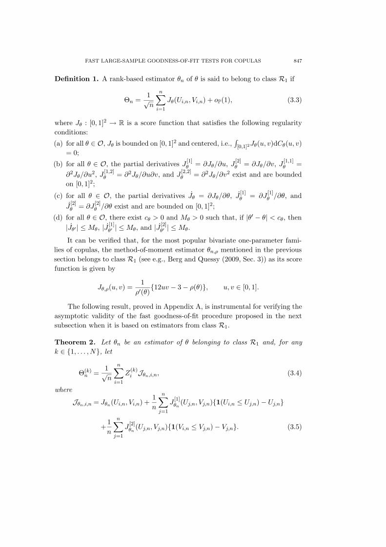
Definition 1. A rank-based estimator θn of θ is said to belong to class R1 if

Θn =1√n

n∑i=1

Jθ(Ui,n, Vi,n) + oP(1), (3.3)

where Jθ : [0, 1]2 → R is a score function that satisfies the following regularityconditions:

(a) for all θ ∈ O, Jθ is bounded on [0, 1]2 and centered, i.e.,∫[0,1]2Jθ(u, v)dCθ(u, v)

= 0;

(b) for all θ ∈ O, the partial derivatives J[1]θ = ∂Jθ/∂u, J

[2]θ = ∂Jθ/∂v, J

[1,1]θ =

∂2Jθ/∂u2, J[1,2]θ = ∂2Jθ/∂u∂v, and J

[2,2]θ = ∂2Jθ/∂v2 exist and are bounded

on [0, 1]2;

(c) for all θ ∈ O, the partial derivatives Jθ = ∂Jθ/∂θ, J[1]θ = ∂J

[1]θ /∂θ, and

J[2]θ = ∂J

[2]θ /∂θ exist and are bounded on [0, 1]2;

(d) for all θ ∈ O, there exist cθ > 0 and Mθ > 0 such that, if |θ′ − θ| < cθ, then|Jθ′ | ≤ Mθ, |J

[1]θ′ | ≤ Mθ, and |J [2]

θ′ | ≤ Mθ.

It can be verified that, for the most popular bivariate one-parameter fami-lies of copulas, the method-of-moment estimator θn,ρ mentioned in the previoussection belongs to class R1 (see e.g., Berg and Quessy (2009, Sec. 3)) as its scorefunction is given by

Jθ,ρ(u, v) =1

ρ′(θ){12uv − 3 − ρ(θ)}, u, v ∈ [0, 1].

The following result, proved in Appendix A, is instrumental for verifying theasymptotic validity of the fast goodness-of-fit procedure proposed in the nextsubsection when it is based on estimators from class R1.

Theorem 2. Let θn be an estimator of θ belonging to class R1 and, for anyk ∈ {1, . . . , N}, let

Θ(k)n =

1√n

n∑i=1

Z(k)i Jθn,i,n, (3.4)

where

Jθn,i,n = Jθn(Ui,n, Vi,n) +1n

n∑j=1

J[1]θn

(Uj,n, Vj,n){1(Ui,n ≤ Uj,n) − Uj,n}

+1n

n∑j=1

J[2]θn

(Uj,n, Vj,n){1(Vi,n ≤ Vj,n) − Vj,n}. (3.5)


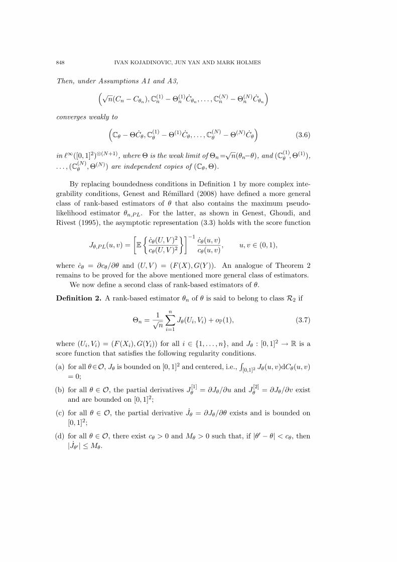
Then, under Assumptions A1 and A3,(√n(Cn − Cθn), C(1)

n − Θ(1)n Cθn , . . . , C(N)

n − Θ(N)n Cθn

)converges weakly to(

Cθ − ΘCθ, C(1)θ − Θ(1)Cθ, . . . , C

(N)θ − Θ(N)Cθ

)(3.6)

in `∞([0, 1]2)⊗(N+1), where Θ is the weak limit of Θn =√

n(θn−θ), and (C(1)θ ,Θ(1)),

. . . , (C(N)θ ,Θ(N)) are independent copies of (Cθ, Θ).

By replacing boundedness conditions in Definition 1 by more complex inte-grability conditions, Genest and Remillard (2008) have defined a more generalclass of rank-based estimators of θ that also contains the maximum pseudo-likelihood estimator θn,PL. For the latter, as shown in Genest, Ghoudi, andRivest (1995), the asymptotic representation (3.3) holds with the score function

Jθ,PL(u, v) =[E

{cθ(U, V )2

cθ(U, V )2

}]−1cθ(u, v)cθ(u, v)

, u, v ∈ (0, 1),

where cθ = ∂cθ/∂θ and (U, V ) = (F (X), G(Y )). An analogue of Theorem 2remains to be proved for the above mentioned more general class of estimators.

We now define a second class of rank-based estimators of θ.

Definition 2. A rank-based estimator θn of θ is said to belong to class R2 if

Θn =1√n

n∑i=1

Jθ(Ui, Vi) + oP(1), (3.7)

where (Ui, Vi) = (F (Xi), G(Yi)) for all i ∈ {1, . . . , n}, and Jθ : [0, 1]2 → R is ascore function that satisfies the following regularity conditions.

(a) for all θ∈O, Jθ is bounded on [0, 1]2 and centered, i.e.,∫[0,1]2 Jθ(u, v)dCθ(u, v)

= 0;

(b) for all θ ∈ O, the partial derivatives J[1]θ = ∂Jθ/∂u and J

[2]θ = ∂Jθ/∂v exist

and are bounded on [0, 1]2;

(c) for all θ ∈ O, the partial derivative Jθ = ∂Jθ/∂θ exists and is bounded on[0, 1]2;

(d) for all θ ∈ O, there exist cθ > 0 and Mθ > 0 such that, if |θ′ − θ| < cθ, then|Jθ′ | ≤ Mθ.


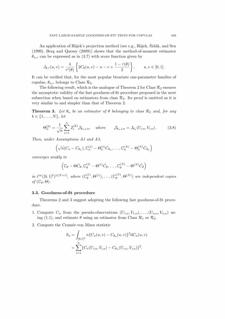
An application of Hajek’s projection method (see e.g., Hajek, Sidak, and Sen(1999), Berg and Quessy (2009)) shows that the method-of-moment estimatorθn,τ can be expressed as in (3.7) with score function given by

Jθ,τ (u, v) =4

τ ′(θ)

{2Cθ(u, v) − u − v +

1 − τ(θ)2

}, u, v ∈ [0, 1].

It can be verified that, for the most popular bivariate one-parameter families ofcopulas, θn,τ belongs to Class R2.

The following result, which is the analogue of Theorem 2 for Class R2 ensuresthe asymptotic validity of the fast goodness-of-fit procedure proposed in the nextsubsection when based on estimators from class R2. Its proof is omitted as it isvery similar to and simpler than that of Theorem 2.

Theorem 3. Let θn be an estimator of θ belonging to class R2 and, for anyk ∈ {1, . . . , N}, let

Θ(k)n =

1√n

n∑i=1

Z(k)i Jθn,i,n, where Jθn,i,n = Jθn(Ui,n, Vi,n). (3.8)

Then, under Assumptions A1 and A3,(√n(Cn − Cθn), C(1)

n − Θ(1)n Cθn , . . . , C(N)

n − Θ(N)n Cθn

)converges weakly to(

Cθ − ΘCθ, C(1)θ − Θ(1)Cθ, . . . , C

(N)θ − Θ(N)Cθ

)in `∞([0, 1]2)⊗(N+1), where (C(1)

θ , Θ(1)), . . . , (C(N)θ , Θ(N)) are independent copies

of (Cθ, Θ).

3.3. Goodness-of-fit procedure

Theorems 2 and 3 suggest adopting the following fast goodness-of-fit proce-dure.

1. Compute Cn from the pseudo-observations (U1,n, V1,n), . . . , (Un,n, Vn,n) us-ing (1.1), and estimate θ using an estimator from Class R1 or R2.

2. Compute the Cramer-von Mises statistic

Sn =∫

[0,1]2n{Cn(u, v) − Cθn(u, v)}2dCn(u, v)

=n∑

i=1

{Cn(Ui,n, Vi,n) − Cθn(Ui,n, Vi,n)}2.


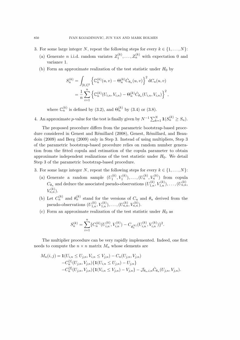
3. For some large integer N , repeat the following steps for every k ∈ {1, . . . , N}:(a) Generate n i.i.d. random variates Z

(k)1 , . . . , Z

(k)n with expectation 0 and

variance 1.

(b) Form an approximate realization of the test statistic under H0 by

S(k)n =

∫[0,1]2

{C(k)

n (u, v) − Θ(k)n Cθn(u, v)

}2dCn(u, v)

=1n

n∑i=1

{C(k)

n (Ui,n, Vi,n) − Θ(k)n Cθn(Ui,n, Vi,n)

}2,

where C(k)n is defined by (3.2), and Θ(k)

n by (3.4) or (3.8).

4. An approximate p-value for the test is finally given by N−1∑N

k=1 1(S(k)n ≥ Sn).

The proposed procedure differs from the parametric bootstrap-based proce-dure considered in Genest and Remillard (2008), Genest, Remillard, and Beau-doin (2009) and Berg (2009) only in Step 3. Instead of using multipliers, Step 3of the parametric bootstrap-based procedure relies on random number genera-tion from the fitted copula and estimation of the copula parameter to obtainapproximate independent realizations of the test statistic under H0. We detailStep 3 of the parametric bootstrap-based procedure.

3. For some large integer N , repeat the following steps for every k ∈ {1, . . . , N}:(a) Generate a random sample (U (k)

1 , V(k)1 ), . . . , (U (k)

n , V(k)n ) from copula

Cθn and deduce the associated pseudo-observations (U (k)1,n , V

(k)1,n ), . . . , (U (k)

n,n,

V(k)n,n ).

(b) Let C(k)n and θ

(k)n stand for the versions of Cn and θn derived from the

pseudo-observations (U (k)1,n , V

(k)1,n ), . . . , (U (k)

n,n, V(k)n,n ).

(c) Form an approximate realization of the test statistic under H0 as

S(k)n =

n∑i=1

{C(k)n (U (k)

i,n , V(k)i,n ) − C

θ(k)n

(U (k)i,n , V

(k)i,n )}2.

The multiplier procedure can be very rapidly implemented. Indeed, one firstneeds to compute the n × n matrix Mn whose elements are

Mn(i, j) = 1(Ui,n ≤ Uj,n, Vi,n ≤ Vj,n) − Cn(Uj,n, Vj,n)

−C [1]n (Uj,n, Vj,n){1(Ui,n ≤ Uj,n) − Uj,n}

−C [2]n (Uj,n, Vj,n){1(Vi,n ≤ Vj,n) − Vj,n} − Jθn,i,nCθn(Uj,n, Vj,n).


Then, to get one approximate realization of the test statistic under the nullhypothesis, it suffices to generate n i.i.d. random variates Z1, . . . , Zn with expec-tation 0 and variance 1, and to perform simple arithmetic operations involvingthe Zi’s and the columns of matrix Mn.

Although an analogue of Theorem 2 and Theorem 3 remains to be provedfor the maximum pseudo-likelihood estimator, we study the finite sample per-formance of the corresponding multiplier goodness-of-fit procedure in the nextsection. Its implementation (in a more general multivariate multiparameter con-text) is the subject of a companion paper (Kojadinovic and Yan (2011)).

4. Finite-sample Performance

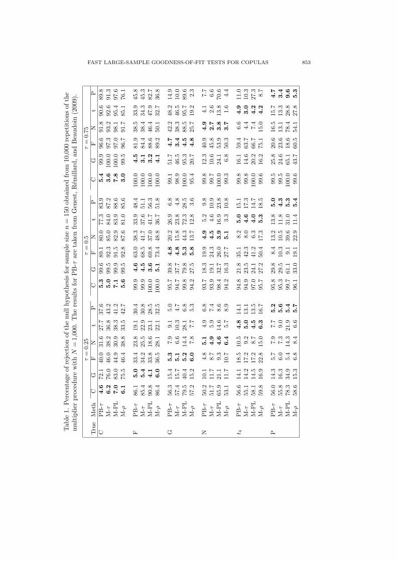
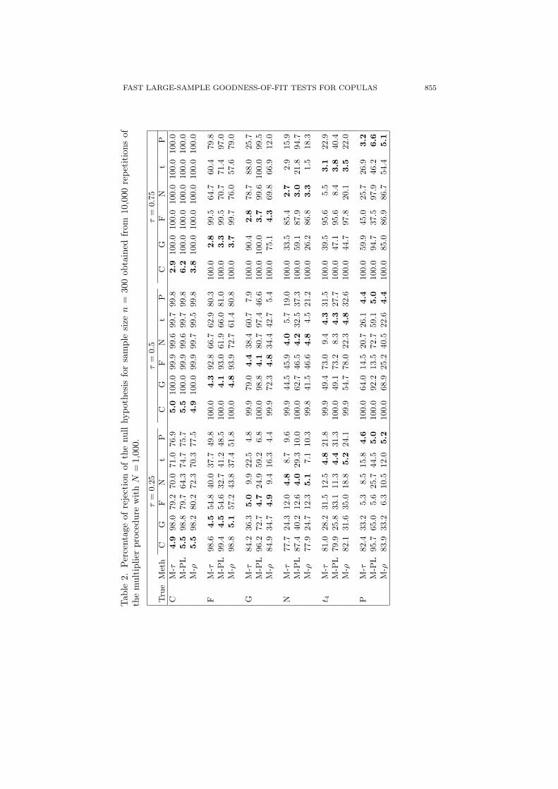
The finite-sample performance of the proposed goodness-of-fit tests was as-sessed in a large-scale simulation study. The experimental design of the studywas very similar to that considered in Genest, Remillard, and Beaudoin (2009).Six bivariate one-parameter families of copulas were considered: the Clayton,Gumbel, Frank, normal, t (with ν = 4 degrees of freedom), and Plackett (seeTable 4 for more details). They are abbreviated as C, G, F, N, t4, and P, respec-tively, in the forthcoming tables. Each one served both as true and hypothesizedcopula. The sample size n = 150 was considered in order to allow a compar-ison with the simulation results presented in Genest, Remillard, and Beaudoin(2009) obtained using the parametric bootstrap-based procedure described in theprevious section in which estimation of the parameter was carried by invertingKendall’s tau. Note that we have not attempted to reproduce these results asthey were obtained after an extensive use of high-performance computing grids.To make this empirical study more insightful, simulations were also carried outfor n = 75 and 300. Three levels of dependence were considered, correspondingto a Kendall’s tau of 0.25, 0.5 and 0.75.

Three multiplier goodness-of-fit tests were compared, differing according tothe method used for estimating the unknown parameter θ of the hypothesizedcopula family. The three tests, based on Kendall’s tau, Spearman’s rho, andmaximum pseudo-likelihood, are abbreviated as M-τ , M-ρ and M-PL. Similarly,the parametric bootstrap procedure based on Kendall’s tau empirically studiedin Genest, Remillard, and Beaudoin (2009) is denoted by PB-τ . In all executionsof the multiplier-based tests, we used standard normal variates for the Zi’s in theprocedure given in Subsection 3.3. As standard normal variates led to satisfactoryresults, we did not investigate the use of other types of multipliers. Also, thenumber of iterations N was fixed to 1,000, equivalent to using 1,000 bootstrapsamples for PB-τ . For each testing scenario, 10,000 repetitions were performedto estimate the level or power of each of the three tests under consideration.


For n = 75 (results not reported), the empirical levels of the three testsappeared overall to be too liberal. As n was increased to 150, the agreementbetween the empirical levels (in bold in Table 1) and the 5% nominal level seemedglobally satisfactory, except for M-PL when data arise from the Clayton copulaor from the Packett copula with τ = 0.75. The empirical levels in Table 2 confirmthat, as the sample size reaches 300, the multiplier approach provided, overall, anaccurate approximation to the null distribution of the test statistics. In terms ofpower, as expected, the rejection percentages increased quite substantially whenn went from 75 to 150, and then to 300.

From Theorems 2 and 3 and the work of Genest and Remillard (2008), weknow that the empirical processes involved in the multiplier and the parametricbootstrap-based tests are asymptotically equivalent if estimation is based on theinversion of Spearman’s rho or Kendall’s tau. The results presented in Table 1for M-τ and PB-τ also suggest that their finite-sample performances are fairlyclose.

From the presented results, it appears that the method chosen for estimatingthe parameter of the hypothesized copula family can greatly influence the powerof the approach. For instance, from Tables 1 and 2, M-PL seems to performparticularly well when the hypothesized copula is the Plackett copula and thedependence is high. The procedure M-PL appears to give the best results overall.It is followed by M-τ .

5. Illustrative Example

The insurance data of Frees and Valdez (1998) are frequently used for illus-tration purposes in copula modeling (see e.g., Klugman and Parsa (1999), Genest,Quessy, and Remillard (2006), Ben Ghorbal, Genest, and Neslehova (2009)). Thetwo variables of interest are an indemnity payment and the corresponding allo-cated loss adjustment expense, and were observed for 1500 claims of an insurancecompany. Following Genest, Quessy, and Remillard (2006), we restrict ourselvesto the 1466 uncensored claims.

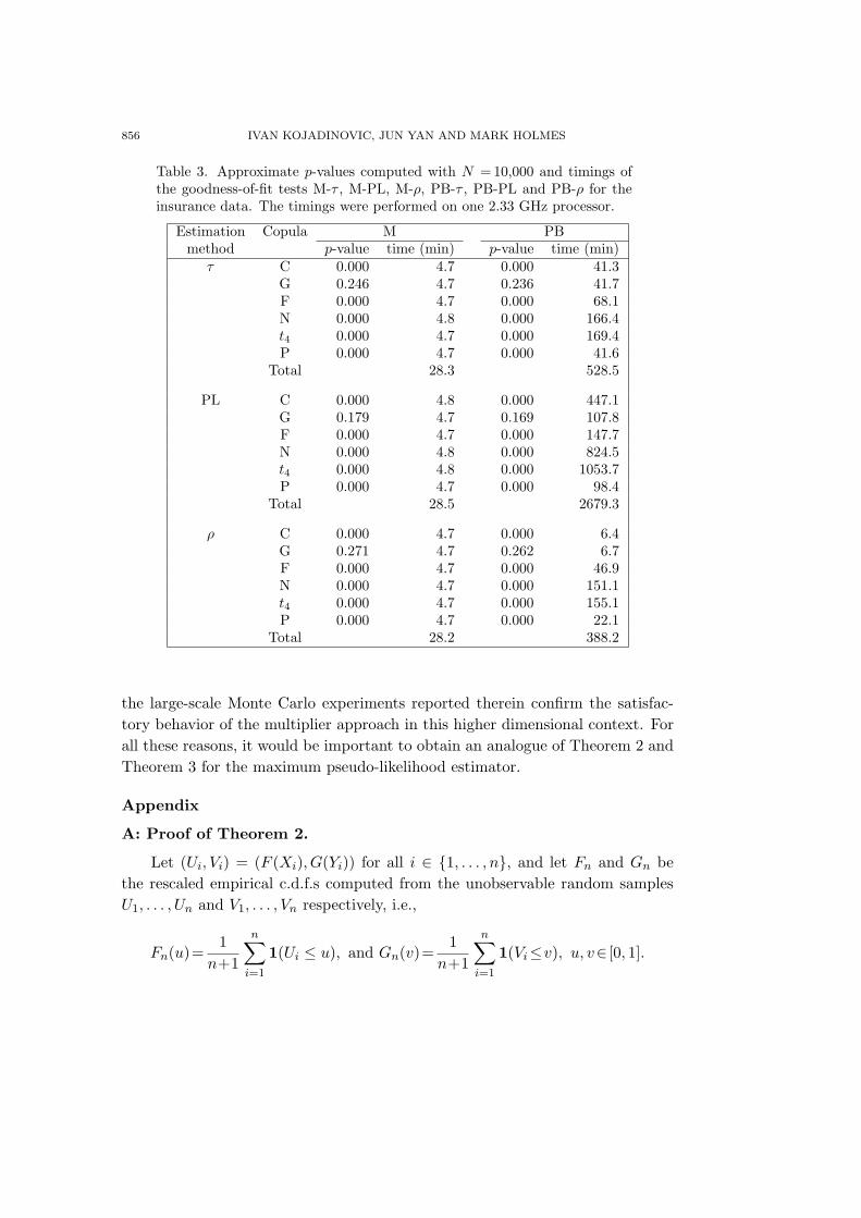
The data under consideration contain a non negligible number of ties. Asdemonstrated in Kojadinovic and Yan (2010b), ignoring the ties, by using forinstance mid-ranks in the computation of the pseudo-observations, may affect theresults qualitatively. For these reasons, when computing the pseudo-observations,we assigned ranks at random in case of ties. This was done using the R functionrank with its argument ties.method set to "random". The random seed thatwe used is 1224. The approximate p-values of the multiplier goodness-of-fit testsand the corresponding parametric bootstrap-based procedures computed withN =10,000 are given in Table 3.

FAST LARGE-SAMPLE GOODNESS-OF-FIT TESTS FOR COPULAS 853Tab

le1.

Per

cent

age

ofre

ject

ion

ofth

enu

llhy

poth

esis

for

sam

ple

size

n=

150

obta

ined

from

10,0

00re

peti

tion

sof

the

mul

tipl

ier

proc

edur

ew

ith

N=

1,00

0.T

here

sult

sfo

rP

B-τ

are

take

nfr

omG

enes

t,R

emill

ard,

and

Bea

udoi

n(2

009)

.

τ=

0.2

5τ

=0.5

τ=

0.7

5Tru

eM

eth

CG

FN

tP

CG

FN

tP

CG

FN

tP

CP

B-τ

4.6

72.1

40.0

31.6

27.7

37.6

5.3

99.6

89.1

80.0

77.3

83.9

5.4

99.9

96.6

91.8

90.6

89.8

M-τ

6.2

76.0

46.0

38.2

36.8

43.2

5.0

99.5

92.3

85.0

84.0

87.2

3.6

100.0

97.3

93.2

92.6

91.3

M-P

L7.0

83.0

44.9

30.9

38.3

41.2

7.1

99.9

91.5

82.9

83.9

88.6

7.8

100.0

97.0

98.1

95.4

97.6

M-ρ

6.1

75.5

46.4

38.8

33.5

42.7

5.6

99.5

92.8

87.6

81.0

85.6

3.0

99.5

96.7

91.7

85.1

76.1

FP

B-τ

86.1

5.0

33.4

23.8

19.1

30.4

99.9

4.6

63.0

38.3

33.9

48.4

100.0

4.5

81.9

38.5

33.9

45.8

M-τ

85.4

5.4

34.2

25.5

22.9

30.8

99.9

4.5

68.5

41.7

37.6

51.1

100.0

3.1

84.4

38.4

34.3

45.3

M-P

L90.8

4.1

33.8

18.6

23.1

28.5

100.0

3.6

69.8

37.0

41.7

56.3

100.0

3.2

88.6

46.4

47.9

82.7

M-ρ

86.4

6.0

36.5

28.1

22.1

32.5

100.0

5.1

73.4

48.8

36.7

51.8

100.0

4.1

89.2

50.1

32.7

36.8

GP

B-τ

56.3

15.4

5.3

7.9

9.1

5.0

95.7

39.8

4.8

20.2

26.9

6.8

99.1

51.7

4.7

42.2

48.2

14.9

M-τ

57.4

15.7

5.1

6.6

10.3

4.7

94.7

37.7

4.8

15.8

23.8

4.8

98.9

46.5

3.4

38.3

46.5

10.0

M-P

L79.5

40.4

5.2

14.4

28.1

6.8

99.8

79.8

5.3

44.3

72.3

28.5

100.0

95.3

4.5

88.5

95.7

89.6

M-ρ

57.2

15.2

6.0

7.8

7.7

5.3

94.2

27.5

5.8

13.7

12.8

3.6

95.4

20.7

4.8

25.7

19.2

2.3

NP

B-τ

50.2

10.1

4.8

5.1

4.9

6.8

93.7

18.3

19.9

4.9

5.2

9.8

99.8

12.3

40.9

4.9

4.1

7.7

M-τ

51.7

11.7

8.7

4.9

5.9

7.4

93.9

19.1

24.3

4.5

4.6

10.9

99.7

10.6

45.8

2.7

2.6

6.6

M-P

L65.9

21.1

9.3

4.6

14.6

8.6

98.4

32.7

26.0

3.9

16.9

23.8

100.0

24.1

53.9

3.8

13.8

70.6

M-ρ

53.1

11.7

10.7

6.4

5.7

8.9

94.2

16.3

27.7

5.1

3.3

10.8

99.3

6.8

50.3

3.7

1.6

4.4

t 4P

B-τ

56.6

14.1

18.5

10.5

4.8

14.1

94.8

21.8

35.1

8.2

5.0

15.1

99.8

16.1

59.4

6.6

4.9

11.0

M-τ

55.1

14.2

17.2

9.2

5.0

13.1

94.9

23.5

42.3

8.0

4.6

17.3

99.8

14.6

63.7

4.4

3.0

10.3

M-P

L58.1

14.5

17.2

8.7

4.5

13.5

97.0

24.1

41.2

6.3

4.0

14.7

100.0

20.2

66.7

7.4

4.2

27.3

M-ρ

59.8

16.9

22.8

15.0

6.3

16.7

95.7

27.2

50.4

17.3

5.3

18.5

99.6

16.2

75.1

15.0

4.2

8.7

PP

B-τ

56.0

14.3

5.7

7.9

7.7

5.2

95.8

29.8

8.4

13.2

13.8

5.0

99.5

25.8

20.6

16.5

15.7

4.7

M-τ

55.8

16.3

6.0

7.3

9.0

5.6

95.3

29.5

10.3

10.5

11.8

4.3

99.5

24.6

23.6

13.1

13.3

3.4

M-P

L78.3

34.9

5.4

14.3

21.9

5.4

99.7

61.1

9.1

39.6

31.0

5.3

100.0

65.1

18.6

78.4

28.8

9.6

M-ρ

58.6

15.3

6.8

8.4

6.6

5.7

96.1

33.0

19.1

22.9

11.4

5.4

99.6

43.7

60.5

54.1

27.8

5.3


Among the six bivariate copulas, only the Gumbel family is not rejectedat the 5% significance level, which might be attributed to the extreme valuedependence in the data (Ben Ghorbal, Genest, and Neslehova (2009)). Thisis in accordance with the results obtained e.g., in Chen and Fan (2005) usingpseudo-likelihood ratio tests, or in Genest, Quessy, and Remillard (2006) usinga goodness-of-fit procedure based on Kendall’s transform. In addition to the p-values, the timings, performed on one 2.33 GHz processor, are provided. Theseare based on our mixed R and C implementation of the tests available in thecopula R package. As one can notice, the use of the multiplier tests results in alarge computational gain while the conclusions remain the same.

To ensure that the randomization does not affect the results qualitatively, thetests based on the pseudo-observations computed with ties.method = "random"were performed a large number of times in Kojadinovic and Yan (2010b). The nu-merical summaries presented in the latter study indicate that the randomizationdoes not affect the conclusions qualitatively for these data.

6. Discussion

The previous illustrative example highlights the most important advan-tage of the studied procedures over their parametric bootstrap-based coun-terparts: the former can be much faster. From the simulation results presentedin Section 4, we also expect the multiplier tests to be at least as powerful asthe parametric bootstrap-based ones for larger n. In other words, the pro-posed multiplier procedures appear as appropriate large-sample substitutes tothe parametric bootstrap-based goodness-of-fit tests used in Genest, Remillard,and Beaudoin (2009) and Berg (2009), and studied theoretically in Genest andRemillard (2008).

From a practical perspective, the results presented in Section 4 indicate thatthe multiplier approach can be safely used even in the case of samples of size assmall as 150 as long as estimation is based on Kendall’s tau or Spearman’s rho.As n reaches 300, all three tests, included the one based on the maximization ofthe pseudo-likelihood, appear to hold their nominal level. The latter version ofthe test also seems to be the most powerful in general.

From the timings presented in the previous section, we see that the computa-tional gain resulting from the use of the multiplier approach appears to be muchmore pronounced when estimation is based on the maximization of the pseudo-likelihood. This is of particular practical importance as, in a general multivariatemultiparameter context, the latter estimation method becomes the only possiblechoice. The finite-sample performance of the maximum pseudo-likelihood versionof the multiplier test was recently studied in a companion paper for multiparam-eter copulas of dimension 3 and 4 (Kojadinovic and Yan (2011)). The results of


Tab

le2.

Per

cent

age

ofre

ject

ion

ofth

enu

llhy

poth

esis

for

sam

ple

size

n=

300

obta

ined

from

10,0

00re

peti

tion

sof

the

mul

tipl

ier

proc

edur

ew

ith

N=

1,00

0.

τ=

0.2

5τ

=0.5

τ=

0.7

5Tru

eM

eth

CG

FN

tP

CG

FN

tP

CG

FN

tP

CM

-τ4.9

98.0

79.2

70.0

71.0

76.9

5.0

100.0

99.9

99.6

99.7

99.8

2.9

100.0

100.0

100.0

100.0

100.0

M-P

L5.5

98.8

79.7

64.3

74.7

75.7

5.5

100.0

99.9

99.6

99.7

99.8

6.2

100.0

100.0

100.0

100.0

100.0

M-ρ

5.5

98.2

80.2

72.3

70.3

77.5

4.9

100.0

99.9

99.7

99.5

99.8

3.8

100.0

100.0

100.0

100.0

100.0

FM

-τ98.6

4.5

54.8

40.0

37.7

49.8

100.0

4.3

92.8

66.7

62.9

80.3

100.0

2.8

99.5

64.7

60.4

79.8

M-P

L99.4

4.5

54.6

32.7

41.2

48.5

100.0

4.1

93.0

61.9

66.0

81.0

100.0

3.3

99.5

70.7

71.4

97.0

M-ρ

98.8

5.1

57.2

43.8

37.4

51.8

100.0

4.8

93.9

72.7

61.4

80.8

100.0

3.7

99.7

76.0

57.6

79.0

GM

-τ84.2

36.3

5.0

9.9

22.5

4.8

99.9

79.0

4.4

38.4

60.7

7.9

100.0

90.4

2.8

78.7

88.0

25.7

M-P

L96.2

72.7

4.7

24.9

59.2

6.8

100.0

98.8

4.1

80.7

97.4

46.6

100.0

100.0

3.7

99.6

100.0

99.5

M-ρ

84.9

34.7

4.9

9.4

16.3

4.4

99.9

72.3

4.8

34.4

42.7

5.4

100.0

75.1

4.3

69.8

66.9

12.0

NM

-τ77.7

24.3

12.0

4.8

8.7

9.6

99.9

44.5

45.9

4.0

5.7

19.0

100.0

33.5

85.4

2.7

2.9

15.9

M-P

L87.4

40.2

12.6

4.0

29.3

10.0

100.0

62.7

46.5

4.2

32.5

37.3

100.0

59.1

87.9

3.0

21.8

94.7

M-ρ

77.9

24.7

12.3

5.1

7.1

10.3

99.8

41.5

46.6

4.8

4.5

21.2

100.0

26.2

86.8

3.3

1.5

18.3

t 4M

-τ81.0

28.2

31.5

12.5

4.8

21.8

99.9

49.4

73.0

9.4

4.3

31.5

100.0

39.5

95.6

5.5

3.1

22.9

M-P

L79.9

25.8

33.1

11.3

4.4

31.3

100.0

49.1

73.2

8.3

4.3

27.7

100.0

47.1

95.6

8.4

3.8

40.4

M-ρ

82.1

31.6

35.0

18.8

5.2

24.1

99.9

54.7

78.0

22.3

4.8

32.6

100.0

44.7

97.8

20.1

3.5

22.0

PM

-τ82.4

33.2

5.3

8.5

15.8

4.6

100.0

64.0

14.5

20.7

26.1

4.4

100.0

59.9

45.0

25.7

26.9

3.2

M-P

L95.7

65.0

5.6

25.7

44.5

5.0

100.0

92.2

13.5

72.7

59.1

5.0

100.0

94.7

37.5

97.9

46.2

6.6

M-ρ

83.9

33.2

6.3

10.5

12.0

5.2

100.0

68.9

25.2

40.5

22.6

4.4

100.0

85.0

86.9

86.7

54.4

5.1


Table 3. Approximate p-values computed with N = 10,000 and timings ofthe goodness-of-fit tests M-τ , M-PL, M-ρ, PB-τ , PB-PL and PB-ρ for theinsurance data. The timings were performed on one 2.33 GHz processor.

Estimation Copula M PBmethod p-value time (min) p-value time (min)

τ C 0.000 4.7 0.000 41.3G 0.246 4.7 0.236 41.7F 0.000 4.7 0.000 68.1N 0.000 4.8 0.000 166.4t4 0.000 4.7 0.000 169.4P 0.000 4.7 0.000 41.6

Total 28.3 528.5

PL C 0.000 4.8 0.000 447.1G 0.179 4.7 0.169 107.8F 0.000 4.7 0.000 147.7N 0.000 4.8 0.000 824.5t4 0.000 4.8 0.000 1053.7P 0.000 4.7 0.000 98.4

Total 28.5 2679.3

ρ C 0.000 4.7 0.000 6.4G 0.271 4.7 0.262 6.7F 0.000 4.7 0.000 46.9N 0.000 4.7 0.000 151.1t4 0.000 4.7 0.000 155.1P 0.000 4.7 0.000 22.1

Total 28.2 388.2

the large-scale Monte Carlo experiments reported therein confirm the satisfac-tory behavior of the multiplier approach in this higher dimensional context. Forall these reasons, it would be important to obtain an analogue of Theorem 2 andTheorem 3 for the maximum pseudo-likelihood estimator.

Appendix

A: Proof of Theorem 2.

Let (Ui, Vi) = (F (Xi), G(Yi)) for all i ∈ {1, . . . , n}, and let Fn and Gn bethe rescaled empirical c.d.f.s computed from the unobservable random samplesU1, . . . , Un and V1, . . . , Vn respectively, i.e.,

Fn(u)=1

n+1

n∑i=1

1(Ui ≤ u), and Gn(v)=1

n+1

n∑i=1

1(Vi≤v), u, v∈ [0, 1].


It is then easy to verify that, for any i ∈ {1, . . . , n}, Ui,n = Fn(Ui) and Vi,n =Gn(Vi).

The proof of Theorem 2 is based on five lemmas. In their proofs, we havesometimes delayed the use of the conditions stated in Definition 1 so that thereader can identify the difficulties associated with considering the more generalclass of estimators defined in Genest and Remillard (2008, Def. 4).

Lemma 1. Let θn be an estimator of θ belonging to class R1. Then,

Θn =√

n(θn − θ) =1√n

n∑i=1

Jθ(Ui, Vi) +1√n

n∑i=1

J[1]θ (Ui, Vi){Fn(Ui) − Ui}

+1√n

n∑i=1

J[2]θ (Ui, Vi){Gn(Vi) − Vi} + oP(1).

Proof. By the second-order Mean Value Theorem, we have

Jθ{Fn(Ui), Gn(Vi)} = Jθ(Ui, Vi) + J[1]θ (Ui, Vi){Fn(Ui) − Ui}

+J[2]θ (Ui, Vi){Gn(Vi) − Vi} + Ri,n,

where

Ri,n =12J

[1,1]θ (U [1]

i,n, V[1]i,n ){Fn(Ui) − Ui}2 +

12J

[2,2]θ (U [2]

i,n, V[2]i,n ){Gn(Vi) − Vi}2

+J[1,2]θ (U [3]

i,n, V[3]i,n ){Fn(Ui) − Ui}{Gn(Vi) − Vi},

and where, for any k ∈ {1, 2, 3}, U[k]i,n is between Ui and Fn(Ui), and V

[k]i,n is

between Vi and Gn(Vi). Then

1√n

n∑i=1

Jθ{Fn(Ui), Gn(Vi)}

=1√n

n∑i=1

Jθ(Ui, Vi) +1√n

n∑i=1

J[1]θ (Ui, Vi){Fn(Ui) − Ui}

+1√n

n∑i=1

J[2]θ (Ui, Vi){Gn(Vi) − Vi} +

1√n

n∑i=1

Ri,n.

Furthermore,∣∣∣∣∣ 1√n

n∑i=1

Ri,n

∣∣∣∣∣≤ sup

u∈[0,1]|Fn(u) − u| × sup

u∈[0,1]|√

n{Fn(u) − u}| × 12n

n∑i=1

|J [1,1]θ (U [1]

i,n, V[1]i,n )|


+ supv∈[0,1]

|Gn(v) − v| × supv∈[0,1]

|√

n{Gn(v) − v}| × 12n

n∑i=1

|J [2,2]θ (U [2]

i,n, V[2]i,n )|

+ supu∈[0,1]

|Fn(u) − u| × supv∈[0,1]

|√

n{Gn(v) − v}| × 1n

n∑i=1

|J [1,2]θ (U [3]

i,n, V[3]i,n )|.

The result follows from the fact that the second-order derivatives of Jθ arebounded on [0, 1]2, that supu∈[0,1] |

√n{Fn(u)−u}| converges in distribution, and

that supu∈[0,1] |Fn(u) − u| P→ 0.

Lemma 2. Let Jθ be the score function of an estimator of θ belonging to classR1 and, for any i ∈ {1, . . . , n}, let

Jθ,i,n = Jθ(Ui, Vi) +1n

n∑j=1

J[1]θ (Uj , Vj){1(Ui ≤ Uj) − Uj}

+1n

n∑j=1

J[2]θ (Uj , Vj){1(Vi ≤ Vj) − Vj}. (A.1)

Then, for any k ∈ {1, . . . , N}, we have

1√n

n∑i=1

Z(k)i (Jθ,i,n − Jθ,i,n) P→ 0,

where Jθ,i,n is defined as in (3.5) with θn replaced by θ.

Proof. For any i ∈ {1, . . . , n}, let Aθ,i,n = Jθ{Fn(Ui), Gn(Vi)} − Jθ(Ui, Vi), andlet

Bθ,i,n =1n

n∑j=1

J[1]θ {Fn(Uj), Gn(Vj)}[1{Fn(Ui) ≤ Fn(Uj)} − Fn(Uj)]

− 1n

n∑j=1

J[1]θ (Uj , Vj){1(Ui ≤ Uj) − Uj},

and let

B′θ,i,n =

1n

n∑j=1

J[2]θ {Fn(Uj), Gn(Vj)}[1{Gn(Vi) ≤ Gn(Vj)} − Gn(Vj)]

− 1n

n∑j=1

J[2]θ (Uj , Vj){1(Vi ≤ Vj) − Vj}.


Let k ∈ {1, . . . , N}. Then, from (3.5) and (A.1), we obtain

1√n

n∑i=1

Z(k)i (Jθ,i,n − Jθ,i,n)

=1√n

n∑i=1

Z(k)i Aθ,i,n +

1√n

n∑i=1

Z(k)i Bθ,i,n +

1√n

n∑i=1

Z(k)i B′

θ,i,n.

By the Mean Value Theorem, we have

1√n

n∑i=1

Z(k)i Aθ,i,n =

1√n

n∑i=1

Z(k)i J

[1]θ (U [1]

i,n, V[1]i,n ){Fn(Ui) − Ui}

+1√n

n∑i=1

Z(k)i J

[2]θ (U [2]

i,n, V[2]i,n ){Gn(Vi) − Vi},

where, for any k = 1, 2, U[k]i,n (resp. V

[k]i,n ) is between Ui and Fn(Ui) (resp. Vi and

Gn(Vi)). Let Dθ,n = n−1/2∑n

i=1 Z(k)i J

[1]θ (U [1]

i,n, V[1]i,n ){Fn(Ui) − Ui}. It is easy to

check that Dθ,n has mean 0 and variance E(D2θ,n) = n−1

∑ni=1 E[{J [1]

θ (U [1]i,n, V

[1]i,n )}2

{Fn(Ui) − Ui}2]. Then,

E(D2θ,n) ≤ 1

n

n∑i=1

E

[{J [1]

θ (U [1]i,n, V

[1]i,n )}2 × { sup

u∈[0,1]|Fn(u) − u|}2

]

≤ supu,v∈[0,1]

{J [1]θ (u, v)}2 × E

[{ sup

u∈[0,1]|Fn(u) − u|}2

].

The right-hand side tends to 0 as a consequence of the Dominated ConvergenceTheorem. Hence, Dθ,n

P→ 0. Similarly, one has that n−1/2∑n

i=1Z(k)i J

[2]θ (U [2]

i,n, V[2]i,n )

{Gn(Vi) − Vi}P→ 0. It follows that n−1/2

∑ni=1 Z

(k)i Aθ,i,n

P→ 0.It remains to show that n−1/2

∑ni=1 Z

(k)i Bθ,i,n and n−1/2

∑ni=1 Z

(k)i B′

θ,i,n con-verge to zero in probability. First, using the fact that 1{Fn(Ui) ≤ Fn(Uj)} =1(Ui ≤ Uj), notice that Bθ,i,n can be expressed as

Bθ,i,n =1n

n∑j=1

J[1]θ {Fn(Uj), Gn(Vj)} {1(Ui ≤ Uj) − Fn(Uj)}

− 1n

n∑j=1

J[1]θ (Uj , Vj){1(Ui ≤ Uj) − Fn(Uj) + Fn(Uj) − Uj},

which implies that n−1/2∑n

i=1 Z(k)i Bθ,i,n can be rewritten as the difference of


Hθ,n =1√n

n∑i=1

Z(k)i

1n

n∑j=1

[J

[1]θ {Fn(Uj), Gn(Vj)}−J

[1]θ (Uj , Vj)

]{1(Ui≤Uj)−Fn(Uj)}

,

and

H ′θ,n =

1n

n∑j=1

J[1]θ (Uj , Vj){Fn(Uj) − Uj}

[1√n

n∑i=1

Z(k)i

].

Now, Hθ,n can be rewritten as

Hθ,n =1n

n∑j=1

[J

[1]θ {Fn(Uj), Gn(Vj)} − J

[1]θ (Uj , Vj)

]

×

[1√n

n∑i=1

Z(k)i {1(Ui ≤ Uj) − Uj}−{Fn(Uj)−Uj} ×

1√n

n∑i=1

Z(k)i

].

Therefore,

|Hθ,n|

≤

[sup

u∈[0,1]

∣∣∣∣∣ 1√n

n∑i=1

Z(k)i {1(Ui ≤ u) − u}

∣∣∣∣∣ + supu∈[0,1]

|Fn(u) − u| ×

∣∣∣∣∣ 1√n

n∑i=1

Z(k)i

∣∣∣∣∣]

× 1n

n∑j=1

∣∣∣J [1]θ {Fn(Uj), Gn(Vj)} − J

[1]θ (Uj , Vj)

∣∣∣ .

From the Multiplier Central Limit Theorem (see e.g., Kosorok (2008, Thm. 10.1))and the Continuous Mapping Theorem, we have that

supu∈[0,1]

∣∣∣∣∣ 1√n

n∑i=1

Z(k)i {1(Ui ≤ u) − u}

∣∣∣∣∣ Ã supu∈[0,1]

|αθ(u, 1)|.

Furthermore, from the Mean Value Theorem, one can write

1n

n∑j=1

∣∣∣J [1]θ {Fn(Uj), Gn(Vj)} − J

[1]θ (Uj , Vj)

∣∣∣≤ 1

n

n∑j=1

∣∣∣J [1,1]θ (U [1]

j,n, V[1]j,n)

∣∣∣ |Fn(Uj)−Uj |+1n

n∑j=1

∣∣∣J [1,2]θ (U [2]

j,n, V[2]j,n)

∣∣∣ |Gn(Vj)−Vj |,


which implies that

1n

n∑j=1

∣∣∣J [1]θ {Fn(Uj), Gn(Vj)} − J

[1]θ (Uj , Vj)

∣∣∣≤ sup

u∈[0,1]|Fn(u) − u| × 1

n

n∑j=1

∣∣∣J [1,1]θ (U [1]

j,n, V[1]j,n)

∣∣∣+ sup

u∈[0,1]|Gn(u) − u| × 1

n

n∑j=1

∣∣∣J [1,2]θ (U [2]

j,n, V[2]j,n)

∣∣∣ .

Since the second-order derivatives of Jθ are bounded on [0, 1]2, the right-handside converges to 0 in probability and hence Hθ,n

P→ 0. For H ′θ,n, we can write

|H ′θ,n| ≤

∣∣∣∣∣ 1√n

n∑i=1

Z(k)i

∣∣∣∣∣ × supu∈[0,1]

|Fn(u) − u| × 1n

n∑j=1

|J [1]θ (Uj , Vj)|.

It follows that H ′θ,n

P→ 0. By symmetry, n−1/2∑n

i=1 Z(k)i B′

θ,i,nP→ 0.

Lemma 3. Let θn be an estimator of θ belonging to class R1. Then, for anyk ∈ {1, . . . , N}, we have

1√n

n∑i=1

Z(k)i (Jθn,i,n − Jθ,i,n) P→ 0,

where Jθn,i,n is defined in (3.5).

Proof. Let k ∈ {1, . . . , N}. Starting from (3.5), for any i ∈ {1, . . . , n}, one has

Jθn,i,n − Jθ,i,n = Jθn(Ui,n, Vi,n) − Jθ(Ui,n, Vi,n)

+1n

n∑j=1

{J [1]θn

(Uj,n, Vj,n) − J[1]θ (Uj,n, Vj,n)}{1(Ui ≤ Uj) − Uj,n}

+1n

n∑j=1

{J [2]θn

(Uj,n, Vj,n) − J[2]θ (Uj,n, Vj,n)}{1(Vi ≤ Vj) − Vj,n}.

From the Mean-Value Theorem, for any i ∈ {1, . . . , n}, there exist θi,n, θ′i,n andθ′′i,n between θ and θn such that

Jθn,i,n − Jθ,i,n

= Jθi,n(Ui,n, Vi,n)(θn − θ) +

1n

n∑j=1

J[1]θ′j,n

(Uj,n, Vj,n)(θn − θ){1(Ui ≤ Uj) − Uj,n}


+1n

n∑j=1

J[2]θ′′j,n

(Uj,n, Vj,n)(θn − θ){1(Vi ≤ Vj) − Vj,n}.

It follows that

1√n

n∑i=1

Z(k)i (Jθn,i,n − Jθ,i,n)

= (θn − θ) × 1√n

n∑i=1

Z(k)i Jθi,n

(Ui,n, Vi,n)

+(θn − θ) × 1n

n∑j=1

J[1]θ′j,n

(Uj,n, Vj,n)1√n

n∑i=1

Z(k)i {1(Ui ≤ Uj) − Uj,n}

+(θn − θ) × 1n

n∑j=1

J[2]θ′′j,n

(Uj,n, Vj,n)1√n

n∑i=1

Z(k)i {1(Vi ≤ Vj) − Vj,n}. (A.2)

Let Kn = n−1/2∑n

i=1 Z(k)i Jθi,n

(Ui,n, Vi,n), and let us show that Ln = (θn −θ)Kn

P→ 0. First, define

K ′n =

1√n

n∑i=1

Z(k)i Jθi,n

(Ui,n, Vi,n)1{|Jθi,n(Ui,n, Vi,n)| ≤ Mθ},

and

K ′′n =

1√n

n∑i=1

Z(k)i Jθi,n

(Ui,n, Vi,n)1{|Jθi,n(Ui,n, Vi,n)| > Mθ},

where Mθ is defined in Condition (d) of Definition 1. Clearly, Kn = K ′n + K ′′

n.Let us now show that K ′′

nP→ 0. Let δ > 0 be given. Then, for n sufficiently large,

P(|θn − θ| < cθ) > 1 − δ. Hence,

1 − δ < P(|θn − θ| < cθ) ≤ P

(n∩

i=1

{|θi,n − θ| < cθ}

)

≤ P

(n∩

i=1

{|Jθi,n(Ui,n, Vi,n)| < Mθ}

),

which implies that P(∪n

i=1{1(|Jθi,n(Ui,n, Vi,n)| > Mθ) > 0}

)< δ, which in turn

implies that K ′′n

P→ 0.To show that Ln = (θn−θ)K ′

n+(θn−θ)K ′′n

P→ 0, it therefore remains to showthat (θn − θ)K ′

nP→ 0. Let ε, δ > 0 be given and choose Mδ such M2

θ /M2δ < δ/2.

Then,P(|θn − θ||K ′

n| > ε) ≤ P(|θn − θ| >ε

Mδ) + P(|K ′

n| > Mδ).


Now, let n be sufficiently large so that P(|θn − θ| > ε/Mδ) < δ/2. Furthermore,by Markov’s inequality and the fact that

E(K ′2n ) =

1n

n∑i=1

E[{Jθi,n

(Ui,n, Vi,n)}21{|Jθi,n(Ui,n, Vi,n)| ≤ Mθ}

]≤ M2

θ ,

we have that

P(|K ′n| > Mδ) ≤

E(K ′2n )

M2δ

≤M2

θ

M2δ

<δ

2.

We therefore obtain that LnP→ 0.

To obtain the desired result, it remains to show that the second and thirdterms on the right side of (A.2) converge to 0 in probability. We shall only dealwith the second term as the proof for the third term is similar. First, notice that∣∣∣∣∣∣ 1n

n∑j=1

J[1]θ′j,n

(Uj,n, Vj,n)1√n

n∑i=1

Z(k)i {1(Ui ≤ Uj) − Uj + Uj − Uj,n}

∣∣∣∣∣∣≤ 1

n

n∑j=1

|J [1]θ′j,n

(Uj,n, Vj,n)|

[sup

u∈[0,1]

∣∣∣∣∣ 1√n

n∑i=1

Z(k)i {1(Ui ≤ u) − u}

∣∣∣∣∣+ sup

u∈[0,1]|Fn(u) − u| ×

∣∣∣∣∣ 1√n

n∑i=1

Z(k)i

∣∣∣∣∣]

.

It is easy to verify that the term between square brackets on the right side ofthe previous inequality converges in distribution. To obtain the desired result,it therefore suffices to show that |θn − θ| × n−1

∑nj=1 |J

[1]θ′j,n

(Uj,n, Vj,n)| P→ 0. Letε > 0 be given. Then,

P

|θn − θ| 1n

n∑j=1

|J [1]θ′j,n

(Uj,n, Vj,n)| < ε

≥ P

|θn − θ| <ε

Mθ,1n

n∑j=1

|J [1]θ′j,n

(Uj,n, Vj,n)| ≤ Mθ

≥ P

|θn − θ| <ε

Mθ,

n∩j=1

{|θ′j,n − θ| < cθ}

→ 1.


Lemma 4. Let Jθ be the score function of an estimator of θ belonging to classR1. Then,

1√n

n∑i=1

[1n

n∑j=1

J[1]θ (Uj , Vj){1(Ui ≤ Uj) − Uj}

−∫

[0,1]2J

[1]θ (u, v){1(Ui ≤ u) − u}dCθ(u, v)

]P→ 0,

and1√n

n∑i=1

[1n

n∑j=1

J[2]θ (Uj , Vj){1(Vi ≤ Vj) − Vj}

−∫

[0,1]2J

[2]θ (u, v){1(Vi ≤ v) − v}dCθ(u, v)

]P→ 0.

Proof. It can be verified that the first term and the second term have mean 0and, that the variance of the first term and the variance of the second term tendto zero, which implies that the terms tend to zero in probability.

Lemma 5. Let Jθ be the score function of an estimator of θ belonging to classR1. For any k ∈ {1, . . . , N}, we have

1√n

n∑i=1

Z(k)i

[1n

n∑j=1

J[1]θ (Uj , Vj){1(Ui ≤ Uj) − Uj}

−∫

[0,1]2J

[1]θ (u, v){1(Ui ≤ u) − u}dCθ(u, v)

]P→ 0,

and1√n

n∑i=1

Z(k)i

[1n

n∑j=1

J[2]θ (Uj , Vj){1(Vi ≤ Vj) − Vj}

−∫

[0,1]2J

[2]θ (u, v){1(Vi ≤ v) − v}dCθ(u, v)

]P→ 0.

Proof. The proof is similar to that of Lemma 4.

Proof of Theorem 2. Let αn =√

n(Hn −Cθ), where Hn is the empirical c.d.f.computed from (U1, V1), . . . , (Un, Vn), and, for any k ∈ {1, . . . , N}, let

α(k)n (u, v) =

1√n

n∑i=1

Z(k)i {1(Ui ≤ u, Vi ≤ v) − Cθ(u, v)} , u, v ∈ [0, 1].


From the results given on page 383 of Remillard and Scaillet (2009) and theMultiplier Central Limit Theorem (see e.g., Kosorok (2008, Thm. 10.1)), wehave that (

αn, α(1)n , α(1)

n , . . . , α(N)n , α(N)

n

)converges weakly to (

αθ, α(1)θ , α

(1)θ , . . . , α

(N)θ , α

(N)θ

)in (`∞([0, 1]2))⊗2N+1, where α

(k)n is defined in (3.1), and α

(1)θ , . . . , α

(N)θ are inde-

pendent copies of αθ. Furthermore, from Lemma 1 and Lemma 4, we have thatΘn = Θn + oP (1), where Θn = n−1/2

∑ni=1 Jθ,i, and where

Jθ,i = Jθ(Ui, Vi) +∫

[0,1]2J

[1]θ (u, v){1(Ui ≤ u) − u}dCθ(u, v)

+∫

[0,1]2J

[2]θ (u, v){1(Vi ≤ v) − v}dCθ(u, v).

Similarly, from Lemmas 2 and 3, we obtain that Θ(k)n and n−1/2

∑ni=1 Z

(k)i Jθ,i,n

are asymptotically equivalent, where Jθ,i,n is defined by (A.1). Then, fromLemma 5, it follows that Θ(k)

n and Θ(k)n = n−1/2

∑ni=1 Z

(k)i Jθ,i are asymptoti-

cally equivalent. Hence,(αn(u, v), Θn, α(1)

n (u, v), Θ(1)n , . . . , α(N)

n (u, v), Θ(N)n

)=

(αn(u, v), Θn, α(1)

n (u, v), Θ(1)n , . . . , α(N)

n (u, v), Θ(N)n

)+ Rn(u, v), (A.3)

where sup(u,v)∈[0,1]2 |Rn(u, v)| P→ 0. Now, (αn(u, v), Θn, α(1)n (u, v), Θ(1)

n , . . .,

α(N)n (u, v), Θ(N)

n ) can be written as the sum of i.i.d. random vectors

1√n

n∑i=1

({1(Ui ≤ u, Vi ≤ v)−Cθ(u, v)}, Jθ,i, Z

(1)i {1(Ui ≤ u, Vi ≤ v)−Cθ(u, v)},

Z(1)i Jθ,i, . . . , Z

(N)i {1(Ui ≤ u, Vi ≤ v) − Cθ(u, v)}, Z(N)

i Jθ,i

),

which, from the Multivariate Central Limit Theorem, converges in distributionto (

αθ(u, v), Θ, α(1)θ (u, v), Θ(1), . . . , α

(N)θ (u, v), Θ(N)

),

where (α(1)θ (u, v), Θ(1)), . . . , (α(N)

θ (u, v), Θ(N)) are independent copies of (αθ(u, v),Θ). Similarly, for any finite collection of points (u1, v1), . . . , (uk, vk) in [0, 1]2,

866 IVAN KOJADINOVIC, JUN YAN AND MARK HOLMES(αn(u1, v1), . . . , αn(uk, vk), Θn, α(1)

n (u1, v1), . . . , α(1)n (uk, vk), Θ(1)

n , . . .

. . . α(N)n (u1, v1), . . . , α(N)

n (uk, vk), Θ(N)n

)converges in distribution, i.e., we have convergence of the finite dimensional dis-tributions. Tightness follows from the fact that αn and α

(k)n each converge weakly

in `∞([0, 1]2), so we obtain that(αn, Θn, α(1)

n , Θ(1)n , . . . , α(N)

n , Θ(N)n

)Ã

(αθ, Θ, α

(1)θ ,Θ(1), . . . , α

(N)θ , Θ(N)

)in (`∞([0, 1]2) ⊗ R)⊗N+1. It follows from (A.3) that(

αn, Θn, α(1)n , Θ(1)

n , . . . , α(N)n ,Θ(N)

n

)Ã

(αθ, Θ, α

(1)θ ,Θ(1), . . . , α

(N)θ , Θ(N)

)in (`∞([0, 1]2) ⊗ R)⊗N+1. Then, from the Continuous Mapping Theorem,(

αn(u, v) − C[1]θ (u, v)αn(u, 1) − C

[2]θ (u, v)αn(1, v) − ΘnCθ(u, v),

α(1)n (u, v) − C

[1]θ (u, v)α(1)

n (u, 1) − C[2]θ (u, v)α(1)

n (1, v) − Θ(1)n Cθ(u, v),

...

α(N)n (u, v) − C

[1]θ (u, v)α(N)

n (u, 1) − C[2]θ (u, v)α(N)

n (1, v) − Θ(N)n Cθ(u, v)

)converges weakly to (3.6) in `∞([0, 1]2)⊗(N+1). Now, from the work of Stute(1984, p.371) (see also Tsukahara (2005, Prop. 1)), we have that

√n{Cn(u, v) − Cθ(u, v)}= αn(u, v) − C

[1]θ (u, v)αn(u, 1) − C

[2]θ (u, v)αn(1, v) + Qn(u, v),

where sup(u,v)∈[0,1]2 |Qn(u, v)| P→ 0. Furthermore, from the work of Quessy (2005,p.73) and under Assumption A3, we can write

√n{Cθn(u, v) − Cθ(u, v)} = ΘnCθ(u, v) + Tn(u, v),

where sup(u,v)∈[0,1]2 |Tn(u, v)| P→ 0. It follows that√

n{Cn(u, v)−Cθn(u, v)} =√

n{Cn(u, v)−Cθ(u, v)}−√

n{Cθn(u, v)−Cθ(u, v)}= αn(u, v) − C

[1]θ (u, v)αn(u, 1) − C

[2]θ (u, v)αn(1, v)

−ΘnCθ(u, v) + Qn(u, v) − Tn(u, v).

Using the fact that C[1]n and C

[2]n converge uniformly in probability to C

[1]θ and

C[1]θ , respectively (Remillard and Scaillet (2009, Prop. A.2)), and the fact that,


Tab

le4.

C.d

.f.s,

Ken

dall’

sta

uan

dSp

earm

an’s

rho

forth

eon

e-pa

ram

eter

copu

lafa

mili

esco

nsid

ered

inth

esi

mul

atio

nst

udy.

The

func

tion

sD

1an

dD

2us

edin

the

expr

essi

ons

ofK

enda

ll’s

tau

and

Spea

rman

’srh

ofo

rth

eFr

ank

copu

laar

eth

eso

-cal

led

first

and

seco

ndD

ebye

func

tion

s(s

eee.

g.G

enes

t,19

87).

Fam

ily

C.d

.f.C

θofth

eco

pula

Para

met

erra

nge

Ken

dall’s

tau

Spea

rman’s

rho

Cla

yto

n“

u−

θ+

v−

θ−

1”

−1/θ

(0,+

∞)

θ

θ+

2N

um

eric

alappro

xim

ati

on

Gum

bel

exp

−“

(−lo

gu)θ

+(−

log

v)θ

”

1/θff

[1,+

∞)

1+

1 θN

um

eric

alappro

xim

ati

on

Fra

nk

−1 θ

log

„

1+

(exp(−

θu)−

1)(

exp(−

θv)−

1)

(exp(−

θ)−

1)

«

R\{0

}1−

4 θ[D

1(−

θ)−

1]

1−

12 θ

[D2(−

θ)−

D1(−

θ)]

Pla

cket

t1

2(θ

−1)

n

1+

(θ−

1)(

u+

v)

[0,+

∞)

Num

eric

alappro

x.

θ+

1

θ−

1−

2θlo

gθ

(θ−

1)2

−ˆ

(1+

(θ−

1)(

u+

v))

2+

4uvθ(1

−θ)˜

1/2

o

Norm

al

Φθ(Φ

−1(u

),Φ

−1(v

)),w

her

eΦ

θis

the

biv

ari

ate

standard

nor-

malc.

d.f.w

ith

corr

elati

on

θ,

and

Φis

the

c.d.f.of

the

uni-

vari

ate

standard

norm

al.

[−1,1

]2 π

arc

sin(θ

)6 π

arc

sin

„

θ 2

«

t νt ν

,θ(t

−1

ν(u

),t−

1ν

(v))

,w

her

et ν

,θis

the

biv

ari

ate

standard

tc.

d.f.

wit

hν

deg

rees

of

free

dom

and

corr

elati

on

θ,

and

t νis

the

c.d.f.

of

the

univ

ari

ate

standard

tw

ith

νdeg

rees

of

free

dom

.

[−1,1

]2 π

arc

sin(θ

)N

um

eric

alappro

xim

ati

on


from Assumption A3, Cθn converges uniformly in probability to Cθ, we finallyobtain that(√

n{Cn(u, v) − Cθn(u, v)},

α(1)n (u, v) − C [1]

n (u, v)α(1)n (u, 1) − C [2]

n (u, v)α(1)n (1, v) − Θ(1)

n Cθn(u, v),...

α(N)n (u, v) − C [1]

n (u, v)α(N)n (u, 1) − C [2]

n (u, v)α(N)n (1, v) − Θ(N)

n Cθn(u, v))

also converges weakly to (3.6) in `∞([0, 1]2)⊗(N+1).

B. Computational details

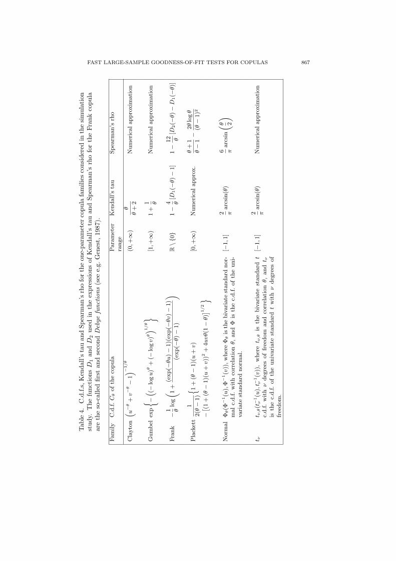
The computations presented in Sections 4 and 5 were performed using theR statistical system (R Development Core Team (2009)) and rely on C code forthe most computationally demanding parts. Table 4, mainly taken from Freesand Valdez (1998), gives the c.d.f.s, Kendall’s tau, and Spearman’s rho for theone-parameter copula families considered in the simulation study. The functionsD1 and D2 used in the expressions of Kendall’s tau and Spearman’s rho for theFrank copula are the so-called first and second Debye functions (see e.g.,Genest(1987)).

B.1. Expressions of τ−1, ρ−1, τ ′ and ρ′

Expressions of τ−1 and ρ−1 required for the moment estimation of the copulaparameter, can be obtained in most cases from the last two columns of Table 4.The same holds for the expressions of τ ′ and ρ′ necessary for computing the scorefunctions Jθ,τ and Jθ,ρ. The following cases are not straightforward.

• For the Frank copula, Spearman’s rho and Kendall’s tau were inverted numer-ically. Furthermore,

ρ′(θ) =12

θ(exp(θ) − 1)− 36

θ2D2(θ) +

24θ2

D1(θ).

• For the Plackett copula, we proceeded as follows. First, using Monte Carlointegration, Kendall’s tau was computed at a dense grid of θ values. Splineinterpolation was then used to compute τ between the grid points. The valuesof τ at the grid points need only to be computed once. The derivative τ ′ wascomputed similarly. More details can be found in Kojadinovic and Yan (2010).

• For the Clayton, Gumbel and t4 copulas, ρ and ρ′ were computed using thesame approach as for Kendall’s tau for the Plackett copula.


B.2. Expressions of Cθ

Only the case of the two meta-elliptical copulas is not immediate. For thebivariate normal copula, the expression of Cθ follows from the so-called Plackettformula (Plackett (1954)):

∂Φθ(x, y)∂θ

=exp

(−(x2 + y2 − 2θxy)/(2(1 − θ2))

)2π

√1 − θ2

,

where Φθ is the bivariate standard normal c.d.f. with correlation θ. The bivariatet generalization of the Plackett formula is given in Genz (2004):

∂tν,θ(x, y)∂θ

=

(1 + (x2 + y2 − 2θxy)/(ν(1 − θ2))

)−ν/2

2π√

1 − θ2,

where tν,θ is the bivariate standard t c.d.f. with ν degrees of freedom and corre-lation θ.

References

Ben Ghorbal, M., Genest, C. and Neslehova, J. (2009). On the test of Ghoudi, Khoudraji, and

Rivest for extreme-value dependence. Canad. J. Statist. 37, 534-552.

Berg, D. (2009). Copula goodness-of-fit testing: An overview and power comparison. Eur. J.

Finance 15, 675-701.

Berg, D. and Quessy, J.-F. (2009). Local sensitivity analyses of goodness-of-fit tests for copulas.

Scand. J. Statist. 36, 389-412.

Chen, X. and Fan, Y. (2005). Pseudo-likelihood ratio tests for semiparametric multivariate

copula model selection. Canad. J. Statist. 33, 389-414.

Cherubini, G., Vecchiato, W. and Luciano, E. (2004). Copula Models in Finance. Wiley, New-

York.

Cui, S. and Sun, Y. (2004). Checking for the gamma frailty distribution under the marginal

proportional hazards frailty model. Statist. Sinica 14, 249-267.

Deheuvels, P. (1981). A non parametric test for independence. Publications de l’Institut de

Statistique de l’Universite de Paris 26, 29-50.

Fermanian, J.-D. (2005). Goodness-of-fit tests for copulas. J. Multivariate Anal. 95, 119-152.

Fermanian, J.-D., Radulovic, D. and Wegkamp, M. (2004). Weak convergence of empirical

copula processes. Bernoulli 10, 847-860.

Fine, J., Yan, J. and Kosorok, M. (2004). Temporal process regression. Biometrika 91, 683-703.

Frees, E. and Valdez, E. (1998). Understanding relationships using copulas. North American

Actuarial J. 2, 1–25.

Ganssler, P. and Stute, W. (1987). Seminar on Empirical Processes. DMV Seminar 9.

Birkhauser, Basel.

Genest, C. (1987). Frank’s family of bivariate distributions. Biometrika 74, 549-555.

Genest, C. and Favre, A.-C. (2007). Everything you always wanted to know about copula

modeling but were afraid to ask. J. Hydrological Engineering 12, 347-368.


Genest, C., Ghoudi, K. and Rivest, L.-P. (1995). A semiparametric estimation procedure ofdependence parameters in multivariate families of distributions. Biometrika 82, 543-552.

Genest, C., Quessy, J.-F. and Remillard, B. (2006). Goodness-of-fit procedures for copulasmodels based on the probability integral transformation. Scand. J. Statist. 33, 337-366.

Genest, C. and Remillard, B. (2008). Validity of the parametric bootstrap for goodness-of-fittesting in semiparametric models. Annales de l’Institut Henri Poincare: Probabilites etStatistiques 44, 1096-1127.

Genest, C., Remillard, B. and Beaudoin, D. (2009). Goodness-of-fit tests for copulas: A reviewand a power study. Insurance: Mathematics and Economics 44, 199-213.

Genz, A. (2004). Numerical computation of rectangular bivariate and trivariate normal and tprobabilities. Statist. Comput. 14, 251-260.

Hajek, J., Sidak, Z. and Sen, P. (1999). Theory of Rank Tests. 2nd edition. Academic Press.

Joe, H. (1997). Multivariate Models and Dependence Concepts. Chapman and Hall, London.

Klugman, S. and Parsa, R. (1999). Fitting bivariate loss distributions with copulas. Insurance:Mathematics and Economics 24, 139-148.

Kojadinovic, I. and Yan, J. (2010). Comparison of three semiparametric methods for estimatingdependence parameters in copula models. Insurance Math. Econom. 47, 52-63.

Kojadinovic, I. and Yan, J. (2011). A goodness-of-fit test for multivariate multiparameter cop-ulas based on multiplier central limit theorems. Statist. Comput. 21, 17-30.

Kojadinovic, I. and Yan, J. (2010b). Modeling multivariate distributions with continuous mar-gins using the copula R package. J. Statist. Software 34, 1-20.

Kosorok, M. (2008). Introduction to Empirical Processes and Semiparametric Inference.Springer, New York.

Lin, D., Fleming, T. and Wei, L. (1994). Confidence bands for survival curves under the pro-portional hazards model. Biometrika 81, 73-81.

McNeil, A., Frey, R. and Embrechts, P. (2005). Quantitative Risk Management. Princeton Uni-versity Press, New Jersey.

Plackett, R. (1954). A reduction formula for normal multivariate probabilities. Biometrika 41,351-369.

Quessy, J.-F. (2005). Methodologie et application des copules: tests d’adequation, testsd’independance, et bornes sur la valeur-a-risque. Ph.D. thesis, Universite Laval, Quebec,Canada.

R Development Core Team (2009). R: A Language and Environment for Statistical Computing.R Foundation for Statistical Computing, Vienna, Austria. ISBN 3-900051-07-0.

Remillard, B. and Scaillet, O. (2009). Testing for equality between two copulas. J. MultivariateAnal. 100, 377-386.

Salvadori, G., Michele, C. D., Kottegoda, N. and Rosso, R. (2007). Extremes in Nature: AnApproach Using Copulas. Water Science and Technology Library, Vol. 56. Springer.

Scaillet, O. (2005). A Kolmogorov-Smirnov type test for positive quadrant dependence. Canad.J. Statist. 33, 415-427.

Shih, J. and Louis, T. (1995). Inferences on the association parameter in copula models forbivariate survival data. Biometrics 51, 1384-1399.

Sklar, A. (1959). Fonctions de repartition a n dimensions et leurs marges. Publications del’Institut de Statistique de l’Universite de Paris 8, 229-231.

Stute, W. (1984). The oscillation behavior of empirical processes: The multivariate case. Ann.Probab. 12, 361-379.


Tsukahara, H. (2005). Semiparametric estimation in copula models. Canad. J. Statist. 33, 357-375.

Yan, J. and Kojadinovic, I. (2010). Copula: Multivariate Dependence with Copulas. R packageversion 0.9-5.

Laboratoire de Mathematiques et Applications, UMR CNRS 5142, Universite de Pau et desPays de l’Adour, 64013 Pau, France.

E-mail: [email protected]

Department of Statistics, University of Connecticut, 215 Glenbrook Rd. U-4120, Storrs, CT06269, USA.


Department of Statistics, The University of Auckland, Private Bag 92019, Auckland 1142, NewZealand.


(Received January 2009; accepted November 2009)

Documents

fast large-sample goodness-of-fit tests for copulas - Institute of