Fast filtering of mobile

signals in radar warning

receiver systems using

machine learning

JORGE ANDRES MUNOZ CACERES

Master in Computer Science

Date: July 10, 2018

Supervisor: Joel Brynielsson

Examiner: Olof Bälter

Swedish title: Maskininlärning för snabb filtrering av mobilsignaler i

radarvarnare

School of Electrical Engineering and Computer Science

Abstract

The radio frequency spectrum is becoming increasingly crowded and

research efforts are being made both from the side of communication

and from radar to allow for sharing of the radio frequency spectrum.

In this thesis, suitable methods for classifying incoming signals as ei-

ther communication signals or radar signals using machine learning

are evaluated, with the purpose of filtering communication signals in

radar warning receiver systems. To this end, a dataset of simulated

communication and radar signals is generated for evaluation. The

methods are evaluated in terms of both accuracy and computational

complexity since both of these aspects are critical in a radar warning

receiver setting. The results show that a deep learning model can be

designed to outperform expert feature-based models in terms of ac-

curacy, as has previously been confirmed in other fields. In terms of

computational complexity, however, they are vastly outperformed by

a model based on ensemble decision trees. As such, a deep learning

model may be too complex for the task of filtering communication sig-

nals from radar signals in a radar warning receiver setting. The classi-

fication accuracy needs to be weighed against the model size and clas-

sification time. Future work should focus on optimizing the feature

extraction implementation for a more fair classification time compari-

son, as well as evaluating the models on recorded data.

Sammanfattning

Radiospektrumet blir alltmer belastat och forskningsinsatser görs in-

om både kommunikation och radar för att tillåta delning av spektru-

met. I denna rapport utvärderas lämpliga metoder för att klassificera

inkommande signaler som antingen kommunikation eller radar med

hjälp av maskininlärning, med syftet att filtrera ut kommunikations-

signaler i radarvarnare. För detta ändamål genereras ett dataset med

simulerade kommunikations- och radarsignaler för att jämföra mo-

dellerna. Metoderna utvärderas med avseende på både precision och

beräkningskomplexitet, eftersom att båda aspekterna är kritiska egen-

skaper i en radarvarnare. Resultaten visar att en djupinlärningsmodell

kan utformas för att överträffa modeller baserade på expertdesigna-

de särdrag med avseende på träffsäkerhet, såsom tidigare visats inom

andra områden. Avseende beräkningskomplexitet, är däremot model-

len baserad på en ensemble av beslutsträd överlägsen. Detta innebär

möjligen att en djupinlärningsmodell är allt för komplex för syftet att

filtrera bort kommunikationssignaler från radarsignaler i en radarvar-

nare. Modellens träffsäkerhet bör vägas mot dess storlek och tiden för

klassificering. Framtida arbete bör inriktas på att optimera beräkning-

en av särdragen för en mer rättvis jämförelse av tiden som krävs för

klassificering, samt att utvärdera modellerna på inspelad data.

Contents

1 Introduction 1

1.1 Purpose . . . . . . . . . . . . . . . . . . . . . . . . . . . . . 2

1.2 Research question . . . . . . . . . . . . . . . . . . . . . . . 2

2 Theory 3

2.1 Signal processing . . . . . . . . . . . . . . . . . . . . . . . 3

2.1.1 Communication signals . . . . . . . . . . . . . . . 4

2.1.2 Radar signals . . . . . . . . . . . . . . . . . . . . . 6

2.1.3 Signal to noise ratio . . . . . . . . . . . . . . . . . . 8

2.2 Feature-based machine learning . . . . . . . . . . . . . . . 9

2.2.1 Decision trees . . . . . . . . . . . . . . . . . . . . . 9

2.2.2 Ensemble learning . . . . . . . . . . . . . . . . . . 10

2.2.3 Support vector machines . . . . . . . . . . . . . . 10

2.2.4 Expert features . . . . . . . . . . . . . . . . . . . . 11

2.3 Deep learning . . . . . . . . . . . . . . . . . . . . . . . . . 14

2.3.1 Artificial neural networks . . . . . . . . . . . . . . 14

2.3.2 Convolutional neural networks . . . . . . . . . . . 15

2.3.3 Residual networks . . . . . . . . . . . . . . . . . . 16

3 Method 18

3.1 Data collection . . . . . . . . . . . . . . . . . . . . . . . . . 18

3.1.1 Mobile signals . . . . . . . . . . . . . . . . . . . . . 19

3.1.2 Radar signals . . . . . . . . . . . . . . . . . . . . . 20

3.1.3 Normalization . . . . . . . . . . . . . . . . . . . . . 20

3.1.4 Dataset generation . . . . . . . . . . . . . . . . . . 21

3.2 Classification models . . . . . . . . . . . . . . . . . . . . . 21

3.2.1 Feature-based machine learning . . . . . . . . . . 22

3.2.2 Deep learning . . . . . . . . . . . . . . . . . . . . . 24

3.3 Experiments . . . . . . . . . . . . . . . . . . . . . . . . . . 25

v

CONTENTS

3.3.1 Accuracy . . . . . . . . . . . . . . . . . . . . . . . . 25

3.3.2 Model complexity . . . . . . . . . . . . . . . . . . 26

4 Results 27

4.1 Accuracy comparison . . . . . . . . . . . . . . . . . . . . . 27

4.2 Model complexity comparison . . . . . . . . . . . . . . . 30

5 Discussion 34

5.1 Accuracy comparison . . . . . . . . . . . . . . . . . . . . . 34

5.2 Model complexity comparison . . . . . . . . . . . . . . . 35

5.3 Radar warning receiver setting . . . . . . . . . . . . . . . 37

6 Conclusions 39

Bibliography 40

vi

Chapter 1

Introduction

The radio spectrum is being used by everything from small Internet of

Things (IoT) devices to large military ships to send and receive data in

different forms. Thus, the Radio Frequency (RF) spectrum is becom-

ing increasingly congested, resulting in a flood of signals being trans-

mitted at all times. This places great demands on devices performing

analysis on signals received over a larger span of the RF spectrum.

One such device is a Radar Warning Receiver (RWR), which is de-

veloped within the field of Electronic Warfare (EW) for analyzing in-

coming RF signals in order to detect and identify hostile radar emit-

ters. By extracting information from the incoming signals it is possible

to determine certain characteristics of the radar emitters, such as lo-

cation and identity, and warn the operators of potential threats. Due

to the congested nature of the RF spectrum, RWR systems can easily

become overwhelmed by the number of incoming signals.

Mobile communication signals are one of the main contributors to

RF spectrum congestion within the context of RWR systems. Mobile

signals are quite strictly regulated in terms of allowed frequencies and

interference levels. Therefore it is tempting to simply filter out the

frequency band allocated to mobile signals. However, this is not a

suitable approach in RWR systems since possibly hostile radar emit-

ters can escape detection by simply using frequency bands originally

allocated to mobile signals. Thus, there is a need for a more powerful

approach to filtering out mobile signals in RWR systems. There are

similarities between this problem and modulation recognition, which

is a problem within the research area of Cognitive Radio (CR), as well

as within radar waveform recognition.

1

CHAPTER 1. INTRODUCTION

Modulation recognition aims to identify the modulation method

used on intercepted mobile signal samples. This is a sub-problem in

the field of CR needed for understanding what communication tech-

nology is being used in order to utilize the same channel without dis-

turbing whoever was already using the channel [33].

Historically research on modulation recognition has focused on de-

veloping and using expert features together with classical Machine

Learning (ML) tools such as Support Vector Machines (SVMs) [30],

decision trees [6] or simpler Artificial Neural Networks (ANNs) [24].

Recently, however, the focus has shifted towards a data-driven Deep

Learning (DL) approach [27] which has previously shown great suc-

cess in other fields, such as image and voice recognition as well as

natural language processing [17].

Automatic radar waveform recognition is a problem within EW

which is very similar to modulation recognition, with the main dif-

ference being the characteristics of communication and radar signals.

As such, different features and algorithms have been employed for

the purpose of radar waveform recognition [22]. The methods emerg-

ing from this field which show most promise are inspired by image

recognition [20] and use Convolutional Neural Networks (CNNs) as

the classification model.

However, there is no published research on distinguishing commu-

nication from radar signals for filtering in an RWR setting.

1.1 Purpose

The purpose of this report is to evaluate methods for automatically

deciding whether an intercepted signal is a communication or a radar

signal with the goal of reducing congestion in devices operating on the

RF spectrum in general and RWRs in particular.

1.2 Research question

How well does a DL approach perform compared to a simpler classifi-

cation model using expert features in terms of accuracy and computa-

tional complexity for the task of classifying communication signals in

RWR systems?

2

Chapter 2

Theory

The first section covers radio signal representation and processing both

in the communication and radar setting. The second section covers the

traditional feature-based ML approach as well as some common fea-

tures used in signal classification. Finally, an overview of ANNs is

given along with a description of the DL approach.

2.1 Signal processing

In signal processing, it is common practice to use a complex-valued,

analytic representation of the real-valued signal as it facilitates many

mathematical operations on the signal [21]. The basic idea is that the

negative components in the Fourier transform of the real-valued func-

tion carries no additional information and can be discarded if one

is willing to deal with a complex-valued function instead. Thus the

analytic representation is the result of calculating the inverse Fourier

transform after discarding the negative components. The real part of

the complex-valued representation is called the I , or In-phase, signal

component, and the imaginary part is called the Q, or Quadrature, sig-

nal component.

These components are best understood with an example. Con-

sider the simple signal s(t) with constant amplitude A and angular

frequency ω,

s(t) = A cosωt, ω > 0.

Then its analytic representation, sa(t), is as follows (for the derivations,

3

CHAPTER 2. THEORY

please refer to the book by Levanon and Mozeson [21]):

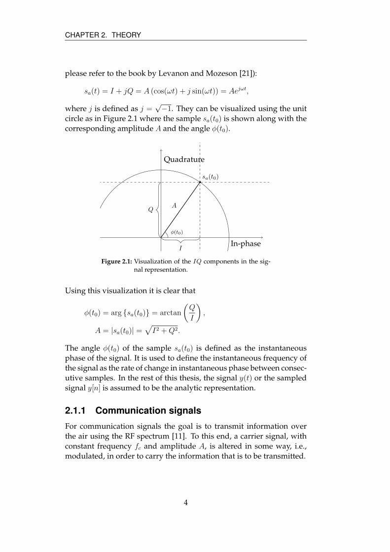
sa(t) = I + jQ = A (cos(ωt) + j sin(ωt)) = Aejωt,

where j is defined as j =√−1. They can be visualized using the unit

circle as in Figure 2.1 where the sample sa(t0) is shown along with the

corresponding amplitude A and the angle φ(t0).

Quadrature

In-phase

A

φ(t0)

sa(t0)

I

Q

Figure 2.1: Visualization of the IQ components in the sig-nal representation.

Using this visualization it is clear that

φ(t0) = arg {sa(t0)} = arctan

(

Q

I

)

,

A = |sa(t0)| =√

I2 +Q2.

The angle φ(t0) of the sample sa(t0) is defined as the instantaneous

phase of the signal. It is used to define the instantaneous frequency of

the signal as the rate of change in instantaneous phase between consec-

utive samples. In the rest of this thesis, the signal y(t) or the sampled

signal y[n] is assumed to be the analytic representation.

2.1.1 Communication signals

For communication signals the goal is to transmit information over

the air using the RF spectrum [11]. To this end, a carrier signal, with

constant frequency fc and amplitude A, is altered in some way, i.e.,

modulated, in order to carry the information that is to be transmitted.

4

CHAPTER 2. THEORY

There are many different kinds of modulation schemes such as

Frequency Modulation (FM), Amplitude Modulation (AM), Phase Shift

Keying (PSK) and Quadrature Amplitude Modulation (QAM). In FM,

the frequency of the carrier signal is altered depending on the infor-

mation to be transmitted. For example, a sound wave can be used

to modulate the frequency of a carrier wave in order to transmit the

sound over long distances. However, since the RF spectrum is very

crowded, especially in urban areas, more efficient ways of modulat-

ing the carrier signals are preferred. Also, the bulk of the information

being transmitted is in the form of binary data, which use digital mod-

ulation schemes.

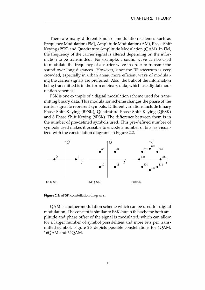
PSK is one example of a digital modulation scheme used for trans-

mitting binary data. This modulation scheme changes the phase of the

carrier signal to represent symbols. Different variations include Binary

Phase Shift Keying (BPSK), Quadrature Phase Shift Keying (QPSK)

and 8 Phase Shift Keying (8PSK). The difference between them is in

the number of pre-defined symbols used. This pre-defined number of

symbols used makes it possible to encode a number of bits, as visual-

ized with the constellation diagrams in Figure 2.2.

Q

I

10

(a) BPSK.

Q

I

0100

10 11

(b) QPSK.

Q

I

001011

101 111

000

010

100

110

(c) 8PSK.

Figure 2.2: nPSK constellation diagrams.

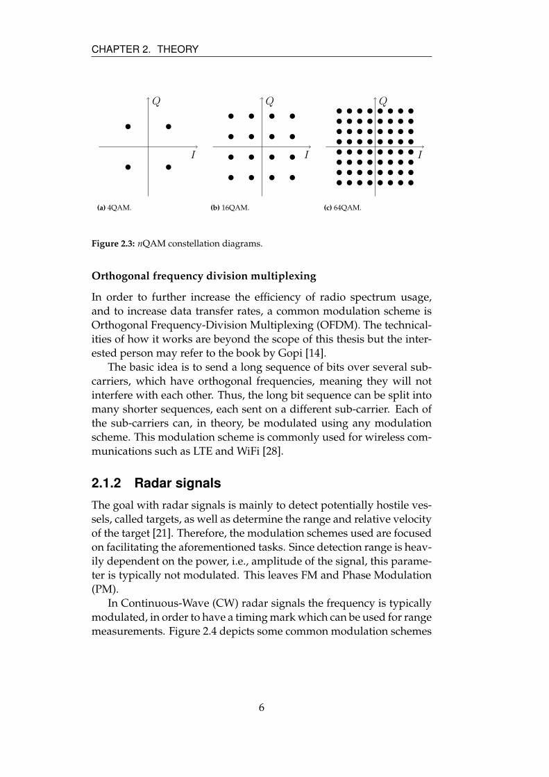
QAM is another modulation scheme which can be used for digital

modulation. The concept is similar to PSK, but in this scheme both am-

plitude and phase offset of the signal is modulated, which can allow

for a larger number of symbol possibilities and more bits per trans-

mitted symbol. Figure 2.3 depicts possible constellations for 4QAM,

16QAM and 64QAM.

5

CHAPTER 2. THEORY

Q

I

(a) 4QAM.

Q

I

(b) 16QAM.

Q

I

(c) 64QAM.

Figure 2.3: nQAM constellation diagrams.

Orthogonal frequency division multiplexing

In order to further increase the efficiency of radio spectrum usage,

and to increase data transfer rates, a common modulation scheme is

Orthogonal Frequency-Division Multiplexing (OFDM). The technical-

ities of how it works are beyond the scope of this thesis but the inter-

ested person may refer to the book by Gopi [14].

The basic idea is to send a long sequence of bits over several sub-

carriers, which have orthogonal frequencies, meaning they will not

interfere with each other. Thus, the long bit sequence can be split into

many shorter sequences, each sent on a different sub-carrier. Each of

the sub-carriers can, in theory, be modulated using any modulation

scheme. This modulation scheme is commonly used for wireless com-

munications such as LTE and WiFi [28].

2.1.2 Radar signals

The goal with radar signals is mainly to detect potentially hostile ves-

sels, called targets, as well as determine the range and relative velocity

of the target [21]. Therefore, the modulation schemes used are focused

on facilitating the aforementioned tasks. Since detection range is heav-

ily dependent on the power, i.e., amplitude of the signal, this parame-

ter is typically not modulated. This leaves FM and Phase Modulation

(PM).

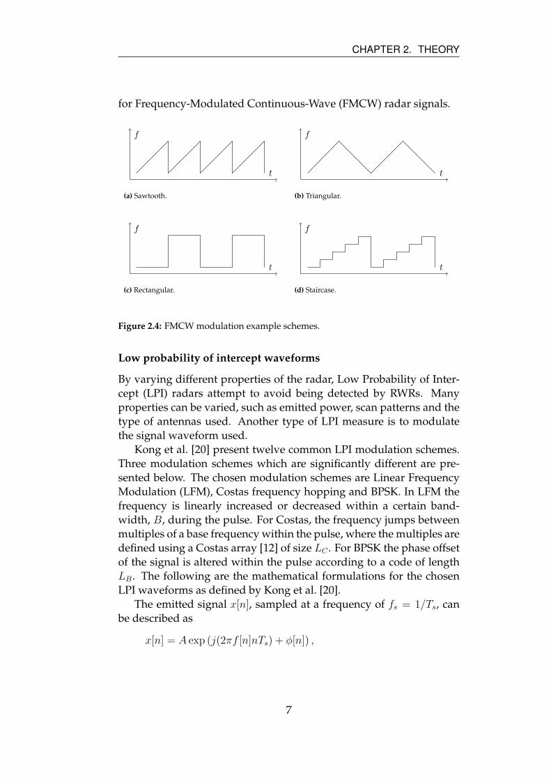
In Continuous-Wave (CW) radar signals the frequency is typically

modulated, in order to have a timing mark which can be used for range

measurements. Figure 2.4 depicts some common modulation schemes

6

CHAPTER 2. THEORY

for Frequency-Modulated Continuous-Wave (FMCW) radar signals.

f

t

(a) Sawtooth.

f

t

(b) Triangular.

f

t

(c) Rectangular.

f

t

(d) Staircase.

Figure 2.4: FMCW modulation example schemes.

Low probability of intercept waveforms

By varying different properties of the radar, Low Probability of Inter-

cept (LPI) radars attempt to avoid being detected by RWRs. Many

properties can be varied, such as emitted power, scan patterns and the

type of antennas used. Another type of LPI measure is to modulate

the signal waveform used.

Kong et al. [20] present twelve common LPI modulation schemes.

Three modulation schemes which are significantly different are pre-

sented below. The chosen modulation schemes are Linear Frequency

Modulation (LFM), Costas frequency hopping and BPSK. In LFM the

frequency is linearly increased or decreased within a certain band-

width, B, during the pulse. For Costas, the frequency jumps between

multiples of a base frequency within the pulse, where the multiples are

defined using a Costas array [12] of size LC . For BPSK the phase offset

of the signal is altered within the pulse according to a code of length

LB. The following are the mathematical formulations for the chosen

LPI waveforms as defined by Kong et al. [20].

The emitted signal x[n], sampled at a frequency of fs = 1/Ts, can

be described as

x[n] = A exp (j(2πf [n]nTs) + φ[n]) ,

7

CHAPTER 2. THEORY

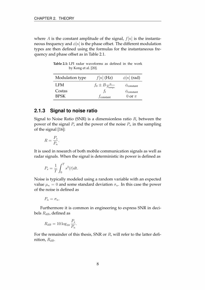
where A is the constant amplitude of the signal, f [n] is the instanta-

neous frequency and φ[n] is the phase offset. The different modulation

types are then defined using the formulas for the instantaneous fre-

quency and phase offset as in Table 2.1.

Table 2.1: LPI radar waveforms as defined in the workby Kong et al. [20].

Modulation type f [n] (Hz) φ[n] (rad)

LFM f0 ± B nNsamps

φconstant

Costas fl φconstant

BPSK fconstant 0 or π

2.1.3 Signal to noise ratio

Signal to Noise Ratio (SNR) is a dimensionless ratio R, between the

power of the signal Ps and the power of the noise Pn in the sampling

of the signal [16]:

R =Ps

Pn

.

It is used in research of both mobile communication signals as well as

radar signals. When the signal is deterministic its power is defined as

Ps =1

T

∫ T

0

s2(t)dt.

Noise is typically modeled using a random variable with an expected

value µn = 0 and some standard deviation σn. In this case the power

of the noise is defined as

Pn = σn.

Furthermore it is common in engineering to express SNR in deci-

bels RdB, defined as

RdB = 10 log10Ps

Pn

.

For the remainder of this thesis, SNR or R, will refer to the latter defi-

nition, RdB.

8

CHAPTER 2. THEORY

2.2 Feature-based machine learning

This section contains the basic theory needed to understand the ap-

proaches based on feature extraction and simple machine learning clas-

sification models. For more detailed explanations, refer to the original

sources.

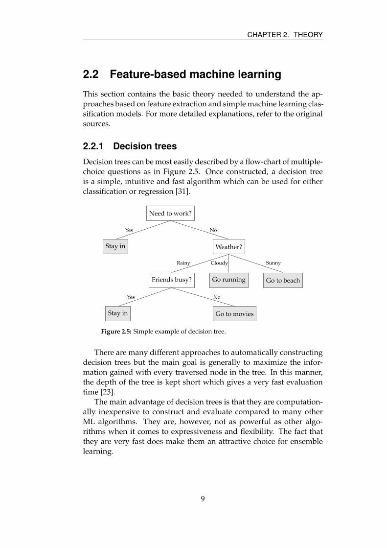
2.2.1 Decision trees

Decision trees can be most easily described by a flow-chart of multiple-

choice questions as in Figure 2.5. Once constructed, a decision tree

is a simple, intuitive and fast algorithm which can be used for either

classification or regression [31].

Need to work?

Stay in Weather?

Friends busy? Go running Go to beach

Stay in Go to movies

Yes No

Rainy Cloudy Sunny

Yes No

Figure 2.5: Simple example of decision tree.

There are many different approaches to automatically constructing

decision trees but the main goal is generally to maximize the infor-

mation gained with every traversed node in the tree. In this manner,

the depth of the tree is kept short which gives a very fast evaluation

time [23].

The main advantage of decision trees is that they are computation-

ally inexpensive to construct and evaluate compared to many other

ML algorithms. They are, however, not as powerful as other algo-

rithms when it comes to expressiveness and flexibility. The fact that

they are very fast does make them an attractive choice for ensemble

learning.

9

CHAPTER 2. THEORY

2.2.2 Ensemble learning

The basic idea behind ensemble learning is that multiple classifiers

might be better than one classifier [23]. This generally holds as long

as the classifiers are independent and diverse. Independence is im-

portant since adding heavily correlated classifiers does not increase

the expressiveness of the ensemble. Diversity is important in order to

be able to capture the variations in the data.

There are multiple methods of ensuring diversity and indepen-

dence of the classifiers when training, the most well-known ones being

boosting and bagging. Bagging is based on generating a new dataset for

every new classifier by randomly choosing points to include from the

original dataset. Boosting involves training classifiers focusing on dif-

ferent parts of available data for every classifier. This can be achieved

by using weights on each input data point as follows.

The first classifier is trained using equal weight for all points. Then

misclassified points are given a larger weight for training the next clas-

sifier. This is repeated until enough classifiers have been trained.

Ensemble training methods are, in theory, applicable to any classifi-

cation algorithm. However, due to the need for training large numbers

of classifiers, simpler models are usually preferred in order to keep the

computational complexity at a reasonable level.

2.2.3 Support vector machines

SVMs are based on the insight that if data is projected into higher-

dimensional space, it usually becomes linearly separable [5]. Thus, the

aim is to project the input data non-linearly into a high-dimensional

space and find a hyperplane in this space to separate the data. The

hyperplane is then represented using a number of data points in the

training data, the support vectors. For classification, the support vectors

are used to determine which side of the hyperplane a new data point

ends up in, and thereby which class it belongs to. Thus the number of

calculations needed for classification is proportional to the number of

support vectors used to represent the hyperplane.

In order to ensure good generalization, the hyperplane should be

placed so that the distance between the plane and positive or negative

data points is maximized. This is called maximizing the margin of

the hyperplane, and is the mathematical problem that is optimized in

SVMs.

10

CHAPTER 2. THEORY

It would be computationally unfeasible to calculate the projections

of each data-point into a high-dimensional space. Especially consider-

ing this space may even have an infinite number of dimensions. This

is where the Kernel trick is applied. A Kernel K, is a function that cal-

culates the result of a dot product between two data-points, K(x1,x2),

when projected to a high-dimensional space, without actually project-

ing the points to this dimension. The most common and successful

kernel function is the Radial Basis Function (RBF) KRBF, defined as

KRBF = exp(−γ||x1 − x2||2),

where γ > 0 is a hyperparameter. The optimization problem used

for SVMs can be reformulated in terms of dot products between data

points which makes it possible to take advantage of the benefits of

high-dimensional spaces without the extensive computational costs

associated with them.

2.2.4 Expert features

As mentioned in Chapter 1, approaches for modulation recognition

have historically been heavily dependent on features designed by ex-

perts in the field, coupled with classification algorithms such as sim-

pler ANNs, SVMs or similar. This is in fact the case for most ML prob-

lems [13].

The DL approach has already surpassed the approach based on ex-

pert features in the fields of image recognition, speech recognition, and

natural language processing [17]. Furthermore, DL has also shown

great promise in the fields of modulation recognition [27] and radar

waveform recognition [20].

Despite these facts, expert features are still worth understanding

and investigating. Firstly, the specific problem being investigated in

this thesis has not been researched previously and expert features can

therefore not be ruled out. Secondly, the inclusion of expert features

may improve the accuracy of a model [4], possibly enabling the use of

simpler models which would result in a low computational complex-

ity. Finally, a very simple classifier coupled with expert features can

serve as a good baseline for comparing to other models.

The following are mathematical descriptions of some of the most

common features used in modulation recognition and radar waveform

11

CHAPTER 2. THEORY

recognition. Note that this section is included for completeness. Un-

derstanding the details in this section is not crucial for understanding

the rest of the thesis.

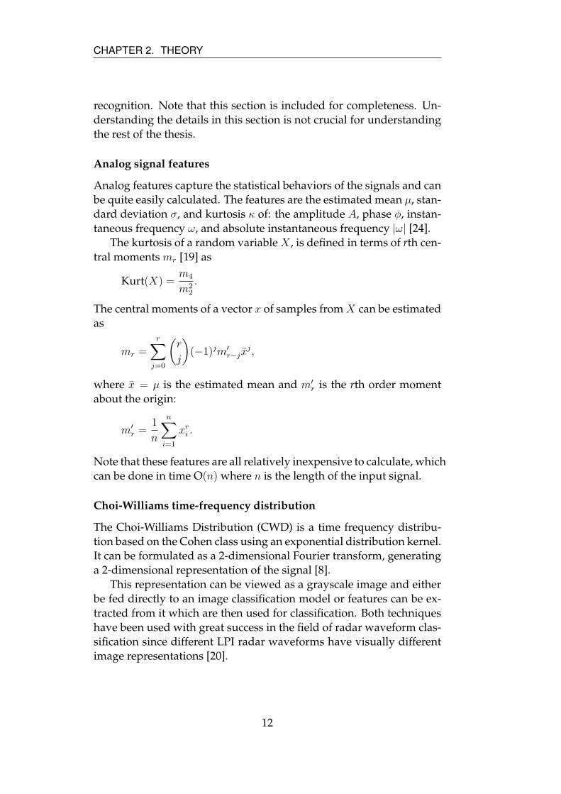
Analog signal features

Analog features capture the statistical behaviors of the signals and can

be quite easily calculated. The features are the estimated mean µ, stan-

dard deviation σ, and kurtosis κ of: the amplitude A, phase φ, instan-

taneous frequency ω, and absolute instantaneous frequency |ω| [24].

The kurtosis of a random variable X , is defined in terms of rth cen-

tral moments mr [19] as

Kurt(X) =m4

m22

.

The central moments of a vector x of samples from X can be estimated

as

mr =r

∑

j=0

(

r

j

)

(−1)jm′r−jx̄

j,

where x̄ = µ is the estimated mean and m′r is the rth order moment

about the origin:

m′r =

1

n

n∑

i=1

xri .

Note that these features are all relatively inexpensive to calculate, which

can be done in time O(n) where n is the length of the input signal.

Choi-Williams time-frequency distribution

The Choi-Williams Distribution (CWD) is a time frequency distribu-

tion based on the Cohen class using an exponential distribution kernel.

It can be formulated as a 2-dimensional Fourier transform, generating

a 2-dimensional representation of the signal [8].

This representation can be viewed as a grayscale image and either

be fed directly to an image classification model or features can be ex-

tracted from it which are then used for classification. Both techniques

have been used with great success in the field of radar waveform clas-

sification since different LPI radar waveforms have visually different

image representations [20].

12

CHAPTER 2. THEORY

Due to the fact that a 2-dimensional Fourier transform is used, there

is a high computational cost for calculating the CWD; O(n3) [20] where

n is the length of the input signal.

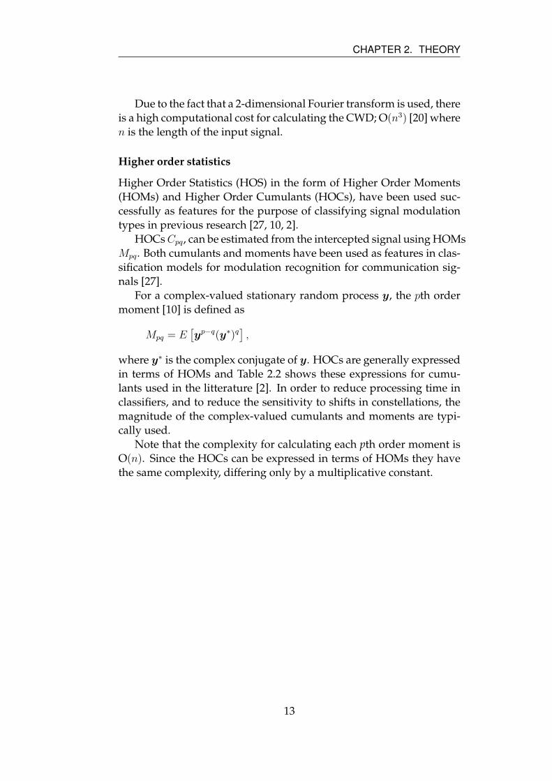
Higher order statistics

Higher Order Statistics (HOS) in the form of Higher Order Moments

(HOMs) and Higher Order Cumulants (HOCs), have been used suc-

cessfully as features for the purpose of classifying signal modulation

types in previous research [27, 10, 2].

HOCs Cpq, can be estimated from the intercepted signal using HOMs

Mpq. Both cumulants and moments have been used as features in clas-

sification models for modulation recognition for communication sig-

nals [27].

For a complex-valued stationary random process y, the pth order

moment [10] is defined as

Mpq = E[

yp−q(y∗)q

]

,

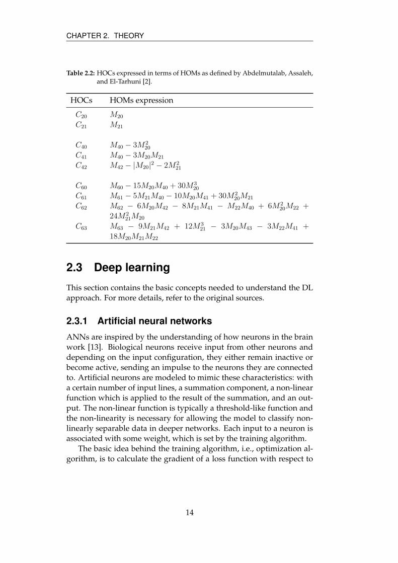
where y∗ is the complex conjugate of y. HOCs are generally expressed

in terms of HOMs and Table 2.2 shows these expressions for cumu-

lants used in the litterature [2]. In order to reduce processing time in

classifiers, and to reduce the sensitivity to shifts in constellations, the

magnitude of the complex-valued cumulants and moments are typi-

cally used.

Note that the complexity for calculating each pth order moment is

O(n). Since the HOCs can be expressed in terms of HOMs they have

the same complexity, differing only by a multiplicative constant.

13

CHAPTER 2. THEORY

Table 2.2: HOCs expressed in terms of HOMs as defined by Abdelmutalab, Assaleh,and El-Tarhuni [2].

HOCs HOMs expression

C20 M20

C21 M21

C40 M40 − 3M220

C41 M40 − 3M20M21

C42 M42 − |M20|2 − 2M221

C60 M60 − 15M20M40 + 30M320

C61 M61 − 5M21M40 − 10M20M41 + 30M220M21

C62 M62 − 6M20M42 − 8M21M41 − M22M40 + 6M220M22 +

24M221M20

C63 M63 − 9M21M42 + 12M321 − 3M20M43 − 3M22M41 +

18M20M21M22

2.3 Deep learning

This section contains the basic concepts needed to understand the DL

approach. For more details, refer to the original sources.

2.3.1 Artificial neural networks

ANNs are inspired by the understanding of how neurons in the brain

work [13]. Biological neurons receive input from other neurons and

depending on the input configuration, they either remain inactive or

become active, sending an impulse to the neurons they are connected

to. Artificial neurons are modeled to mimic these characteristics: with

a certain number of input lines, a summation component, a non-linear

function which is applied to the result of the summation, and an out-

put. The non-linear function is typically a threshold-like function and

the non-linearity is necessary for allowing the model to classify non-

linearly separable data in deeper networks. Each input to a neuron is

associated with some weight, which is set by the training algorithm.

The basic idea behind the training algorithm, i.e., optimization al-

gorithm, is to calculate the gradient of a loss function with respect to

14

CHAPTER 2. THEORY

the weights in the network and update the weights in the direction

specified by the gradient. The loss function is basically a measure of

how well the algorithm performed on the available training data. This

process is repeated for a number of iterations, called epochs. Differ-

ent optimization algorithms exist, one of the most popular being the

Adam optimizer [18]. Optimization algorithms differ mainly in how

the gradient is calculated and how much the weights are updated.

The most simple artificial neural networks are single layer percep-

trons. In this type of network, there are a certain number of input

nodes, one for each dimension in the data, and a certain number of

output nodes, one for each dimension in the output. For this type of

network, the only weights to train are the ones connected to the out-

put nodes. Due to its simplicity, this type of network is only capable

of correctly classifying linearly separable data.

By increasing the number of layers between input and output, data

that is not linearly separable can be classified. Increasing the number

of layers further, and how neurons are connected, allows classification

of more complex patterns in data.

ANNs have been researched since the 1940s, but lately state-of-the-

art results have been surpassed in many fields by the DL approach

for designing and training ANNs. This means designing the network

so that the first few layers have the capability to automatically learn

to extract features from raw input data while the final layers perform

the classification using these features. DL has surpassed the previous

state-of-the-art in image recognition, voice recognition, natural lan-

guage processing and has shown great potential in modulation recog-

nition for both communication and radar signals.

2.3.2 Convolutional neural networks

A convolution can be described as the weighted average between two

functions. Although not all CNNs perform the exact mathematical

definition of a convolution, this is the inspiration for them [13]. This

type of network is useful for reducing the dimension of the data as well

as for processing data that is known to have a grid-like structure. The

typical example is within image recognition, where each individual

pixel value is not as important as the structures formed by neighbor-

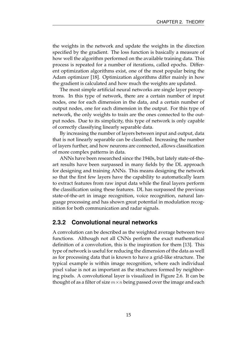
ing pixels. A convolutional layer is visualized in Figure 2.6. It can be

thought of as a filter of size m×n being passed over the image and each

15

CHAPTER 2. THEORY

output value saved in the output layer. The value in the output layer

to the right corresponds to the weighted sum of all the values in the

square to the left, where each position in the filter has a corresponding

weight that is set during training.

Input layer Convolutional layer

Figure 2.6: Visualization of a convolutional layer on an image witha depth of 1.

The number of filters used, m, n, and how much the filter is moved

for each value in the output, i.e., step size, are all hyperparameters

that can be altered. The choice of hyperparameters determines the

number of trainable parameters in the model and thereby the model

complexity and expressiveness.

CNNs have been successfully employed for the task of image recog-

nition and especially so using the DL approach. They are generally

placed early in the network in order to learn translation invariant im-

age features with increasing complexity as each layer is traversed.

2.3.3 Residual networks

As computational capacity increases and new training methods are re-

searched, ANNs have become deeper and deeper. When depth is in-

creased too much, a degradation problem has been observed which is

not connected to overfitting since both training and testing error in-

crease. To address this problem, Residual Networks (RNs) have been

proposed [15]. The intuition is that a deep network should be able to

achieve at least as good performance as a shallow network, since it

16

CHAPTER 2. THEORY

should be possible for the last layers to be the identity mapping and

the rest of the network be equal to the shallow network. As mentioned,

however, deeper networks have shown a degradation problem, which

could suggest that it is difficult for networks to create the identity map-

ping. He et al. [15] propose to make this identity mapping explicit

through the use of shortcut connections, basically connections that by-

pass a number of layers in the network.

This method has allowed the use of deeper networks with the re-

sult of increased accuracy [15]. RNs were also used by O’Shea, Roy,

and Clancy [27] for more shallow networks with great success for mod-

ulation recognition.

17

Chapter 3

Method

The first section describes the dataset used and how it was generated.

The second section describes the classification models, and the last sec-

tion covers the experiments performed.

3.1 Data collection

There are many stages in an RWR at which mobile signal filtering

could be attempted and in this thesis the analytic representation, i.e.,

IQ representation, is investigated for multiple reasons.

As stated in Section 1.1 the purpose of this work is to reduce the

overall congestion. Therefore the filtering should happen as early as

possible to avoid wasting resources on communication signals. Fur-

thermore, communication and radar signals are well-defined in terms

of their IQ representation, but how they appear at later stages in an

RWR depends heavily on the particular implementation. Previous re-

search, presented in Chapter 2, has also focused on classifying the IQ

representations of the signals. Finally, communication and radar sig-

nals are visually very different in their IQ representations for reason-

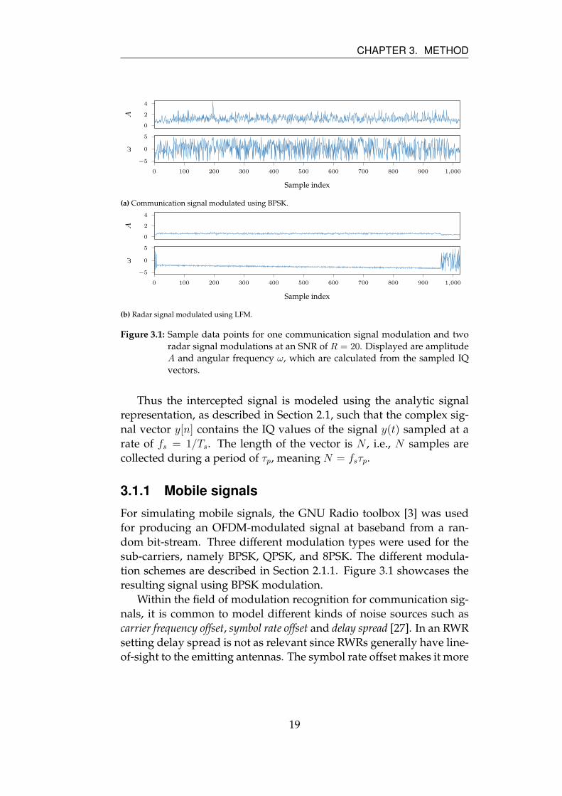
able SNRs, as can be seen in Figure 3.1. This should allow for very

simple and fast classification models, which is crucial in an RWR.

18

CHAPTER 3. METHOD

0

2

4

A

0 100 200 300 400 500 600 700 800 900 1,000

−5

0

5

Sample index

ω

(a) Communication signal modulated using BPSK.

0

2

4

A

0 100 200 300 400 500 600 700 800 900 1,000

−5

0

5

Sample index

ω

(b) Radar signal modulated using LFM.

Figure 3.1: Sample data points for one communication signal modulation and tworadar signal modulations at an SNR of R = 20. Displayed are amplitudeA and angular frequency ω, which are calculated from the sampled IQvectors.

Thus the intercepted signal is modeled using the analytic signal

representation, as described in Section 2.1, such that the complex sig-

nal vector y[n] contains the IQ values of the signal y(t) sampled at a

rate of fs = 1/Ts. The length of the vector is N , i.e., N samples are

collected during a period of τp, meaning N = fsτp.

3.1.1 Mobile signals

For simulating mobile signals, the GNU Radio toolbox [3] was used

for producing an OFDM-modulated signal at baseband from a ran-

dom bit-stream. Three different modulation types were used for the

sub-carriers, namely BPSK, QPSK, and 8PSK. The different modula-

tion schemes are described in Section 2.1.1. Figure 3.1 showcases the

resulting signal using BPSK modulation.

Within the field of modulation recognition for communication sig-

nals, it is common to model different kinds of noise sources such as

carrier frequency offset, symbol rate offset and delay spread [27]. In an RWR

setting delay spread is not as relevant since RWRs generally have line-

of-sight to the emitting antennas. The symbol rate offset makes it more

19

CHAPTER 3. METHOD

difficult to demodulate the signal and extract the transmitted informa-

tion, which is not the goal in this thesis and is therefore not considered.

Thermal noise and carrier frequency offset, however, are relevant and

are modeled using the additive white Gaussian noise channel in the

GNU Radio toolbox.

3.1.2 Radar signals

Two types of radar signals were simulated: FMCW and pulsed radar

signals. For FMCW, the Radar module [32] in the GNU Radio tool-

box [3] was used to generate the signals. The modulation schemes

used were: sawtooth, triangular and rectangular, as described in Sec-

tion 2.1.2.

Pulsed radar signals

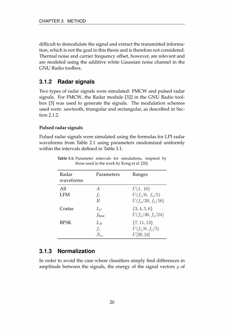
Pulsed radar signals were simulated using the formulas for LPI radar

waveforms from Table 2.1 using parameters randomized uniformly

within the intervals defined in Table 3.1.

Table 3.1: Parameter intervals for simulations, inspired bythose used in the work by Kong et al. [20].

Radar

waveforms

Parameters Ranges

All A U(1, 10)

LFM fc U(fs/6, fs/5)

B U(fs/20, fs/16)

Costas LC {3, 4, 5, 6}fbase U(fs/30, fs/24)

BPSK LB {7, 11, 13}fc U(fs/6, fs/5)

Ncc U [20, 24]

3.1.3 Normalization

In order to avoid the case where classifiers simply find differences in

amplitude between the signals, the energy of the signal vectors y of

20

CHAPTER 3. METHOD

length N = 1024 are normalized as proposed in the work by O’Shea

and West [26]:

yNormn =

ynNµA

, ∀n ∈ 1, 2, . . . , N.

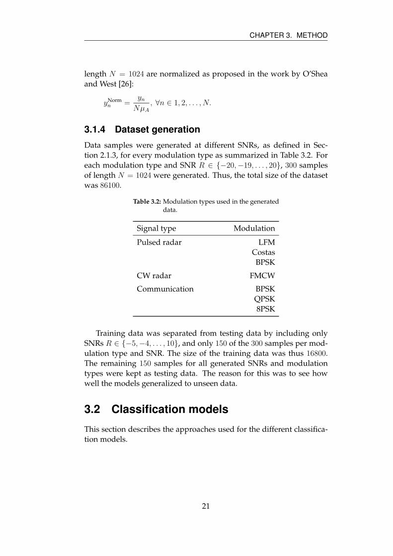
3.1.4 Dataset generation

Data samples were generated at different SNRs, as defined in Sec-

tion 2.1.3, for every modulation type as summarized in Table 3.2. For

each modulation type and SNR R ∈ {−20,−19, . . . , 20}, 300 samples

of length N = 1024 were generated. Thus, the total size of the dataset

was 86100.

Table 3.2: Modulation types used in the generateddata.

Signal type Modulation

Pulsed radar LFM

Costas

BPSK

CW radar FMCW

Communication BPSK

QPSK

8PSK

Training data was separated from testing data by including only

SNRs R ∈ {−5,−4, . . . , 10}, and only 150 of the 300 samples per mod-

ulation type and SNR. The size of the training data was thus 16800.

The remaining 150 samples for all generated SNRs and modulation

types were kept as testing data. The reason for this was to see how

well the models generalized to unseen data.

3.2 Classification models

This section describes the approaches used for the different classifica-

tion models.

21

CHAPTER 3. METHOD

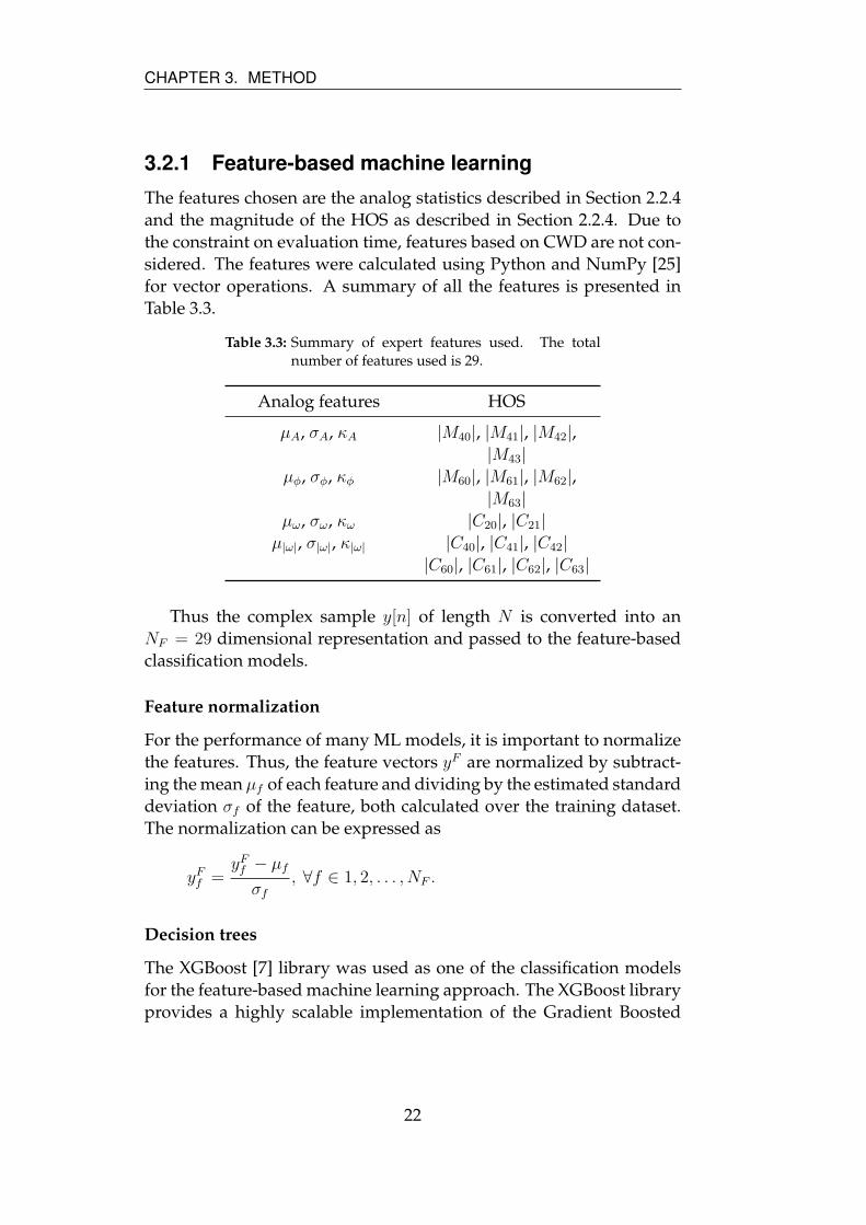
3.2.1 Feature-based machine learning

The features chosen are the analog statistics described in Section 2.2.4

and the magnitude of the HOS as described in Section 2.2.4. Due to

the constraint on evaluation time, features based on CWD are not con-

sidered. The features were calculated using Python and NumPy [25]

for vector operations. A summary of all the features is presented in

Table 3.3.

Table 3.3: Summary of expert features used. The totalnumber of features used is 29.

Analog features HOS

µA, σA, κA |M40|, |M41|, |M42|,|M43|

µφ, σφ, κφ |M60|, |M61|, |M62|,|M63|

µω, σω, κω |C20|, |C21|µ|ω|, σ|ω|, κ|ω| |C40|, |C41|, |C42|

|C60|, |C61|, |C62|, |C63|

Thus the complex sample y[n] of length N is converted into an

NF = 29 dimensional representation and passed to the feature-based

classification models.

Feature normalization

For the performance of many ML models, it is important to normalize

the features. Thus, the feature vectors yF are normalized by subtract-

ing the mean µf of each feature and dividing by the estimated standard

deviation σf of the feature, both calculated over the training dataset.

The normalization can be expressed as

yFf =yFf − µf

σf

, ∀f ∈ 1, 2, . . . , NF .

Decision trees

The XGBoost [7] library was used as one of the classification models

for the feature-based machine learning approach. The XGBoost library

provides a highly scalable implementation of the Gradient Boosted

22

CHAPTER 3. METHOD

Machine (GBM), which is a successful and widely used theoretical

framework for training ensemble tree models. Decision trees and en-

semble methods are described in Sections 2.2.1 and 2.2.2 respectively.

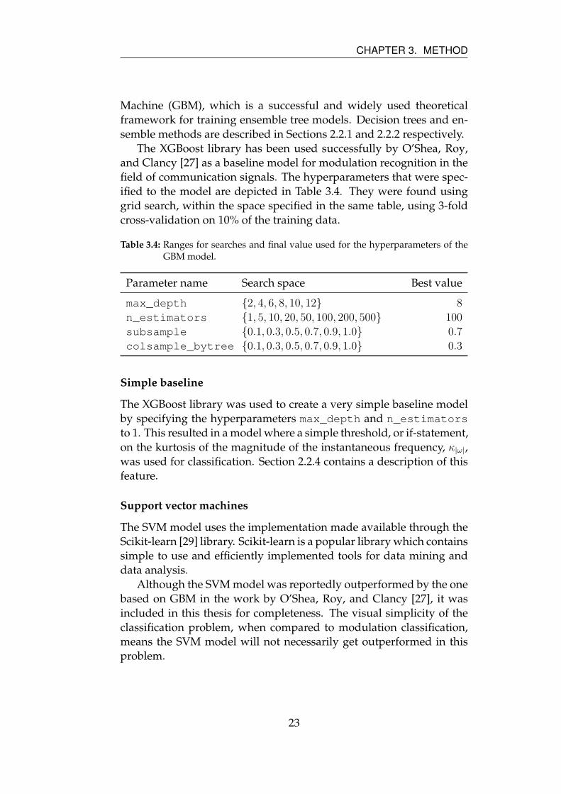
The XGBoost library has been used successfully by O’Shea, Roy,

and Clancy [27] as a baseline model for modulation recognition in the

field of communication signals. The hyperparameters that were spec-

ified to the model are depicted in Table 3.4. They were found using

grid search, within the space specified in the same table, using 3-fold

cross-validation on 10% of the training data.

Table 3.4: Ranges for searches and final value used for the hyperparameters of theGBM model.

Parameter name Search space Best value

max_depth {2, 4, 6, 8, 10, 12} 8

n_estimators {1, 5, 10, 20, 50, 100, 200, 500} 100

subsample {0.1, 0.3, 0.5, 0.7, 0.9, 1.0} 0.7

colsample_bytree {0.1, 0.3, 0.5, 0.7, 0.9, 1.0} 0.3

Simple baseline

The XGBoost library was used to create a very simple baseline model

by specifying the hyperparameters max_depth and n_estimators

to 1. This resulted in a model where a simple threshold, or if-statement,

on the kurtosis of the magnitude of the instantaneous frequency, κ|ω|,

was used for classification. Section 2.2.4 contains a description of this

feature.

Support vector machines

The SVM model uses the implementation made available through the

Scikit-learn [29] library. Scikit-learn is a popular library which contains

simple to use and efficiently implemented tools for data mining and

data analysis.

Although the SVM model was reportedly outperformed by the one

based on GBM in the work by O’Shea, Roy, and Clancy [27], it was

included in this thesis for completeness. The visual simplicity of the

classification problem, when compared to modulation classification,

means the SVM model will not necessarily get outperformed in this

problem.

23

CHAPTER 3. METHOD

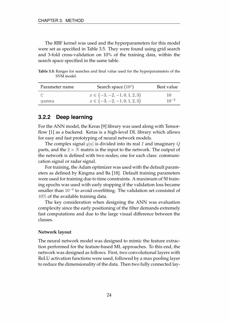
The RBF kernel was used and the hyperparameters for this model

were set as specified in Table 3.5. They were found using grid search

and 3-fold cross-validation on 10% of the training data, within the

search space specified in the same table.

Table 3.5: Ranges for searches and final value used for the hyperparameters of theSVM model.

Parameter name Search space (10x) Best value

C x ∈ {−3,−2,−1, 0, 1, 2, 3} 10

10−2gamma x ∈ {−3,−2,−1, 0, 1, 2, 3}

3.2.2 Deep learning

For the ANN model, the Keras [9] library was used along with Tensor-

flow [1] as a backend. Keras is a high-level DL library which allows

for easy and fast prototyping of neural network models.

The complex signal y[n] is divided into its real I and imaginary Q

parts, and the 2×N matrix is the input to the network. The output of

the network is defined with two nodes; one for each class: communi-

cation signal or radar signal.

For training, the Adam optimizer was used with the default param-

eters as defined by Kingma and Ba [18]. Default training parameters

were used for training due to time constraints. A maximum of 50 train-

ing epochs was used with early stopping if the validation loss became

smaller than 10−4 to avoid overfitting. The validation set consisted of

10% of the available training data.

The key consideration when designing the ANN was evaluation

complexity since the early positioning of the filter demands extremely

fast computations and due to the large visual difference between the

classes.

Network layout

The neural network model was designed to mimic the feature extrac-

tion performed for the feature-based ML approaches. To this end, the

network was designed as follows. First, two convolutional layers with

ReLU activation functions were used, followed by a max pooling layer

to reduce the dimensionality of the data. Then two fully connected lay-

24

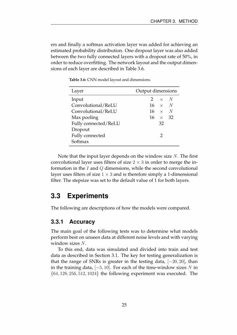
CHAPTER 3. METHOD

ers and finally a softmax activation layer was added for achieving an

estimated probability distribution. One dropout layer was also added

between the two fully connected layers with a dropout rate of 50%, in

order to reduce overfitting. The network layout and the output dimen-

sions of each layer are described in Table 3.6.

Table 3.6: CNN model layout and dimensions.

Layer Output dimensions

Input 2 × N

16 × N

16 × N

16 × 32

32

2

Convolutional/ReLU

Convolutional/ReLU

Max pooling

Fully connected/ReLU

Dropout

Fully connected

Softmax

Note that the input layer depends on the window size N . The first

convolutional layer uses filters of size 2 × 3 in order to merge the in-

formation in the I and Q dimensions, while the second convolutional

layer uses filters of size 1 × 3 and is therefore simply a 1-dimensional

filter. The stepsize was set to the default value of 1 for both layers.

3.3 Experiments

The following are descriptions of how the models were compared.

3.3.1 Accuracy

The main goal of the following tests was to determine what models

perform best on unseen data at different noise levels and with varying

window sizes N .

To this end, data was simulated and divided into train and test

data as described in Section 3.1. The key for testing generalization is

that the range of SNRs is greater in the testing data, [−20, 20], than

in the training data, [−5, 10]. For each of the time-window sizes N in

{64, 128, 256, 512, 1024} the following experiment was executed. The

25

CHAPTER 3. METHOD

models were trained on all available training data and then the total

test set accuracy was recorded for each model and noise level in the

data. Due to the stochasticity in the model initialization, particularly

for the CNN model, the experiment was repeated 20 times and the

average accuracy was calculated and recorded.

To get different window sizes, the same generated data was used

by selecting a window of length N from each sample. This window

was chosen to start at a random index from the original sample of

length N = 1024. The index was sampled from a uniform distribution

and all the samples of the same window size used the same starting

index.

3.3.2 Model complexity

In order to evaluate the relative performance of the models in terms of

computational complexity each model was first trained as described in

Section 3.3.1. During classification, the execution time for classifying

all the samples in the test set was measured and an average classi-

fication time per sample was calculated. This process was repeated

10 times and the average time was recorded. The same window sizes

were used as in previous experiments to see how the models scale with

window size.

The execution time for feature extraction was measured separately

in order to not weigh down the actual models but still allow for com-

paring the time taken for different window sizes.

The implementation of the SVM model only uses a single core on

the CPU as opposed to the other models which can either use multiple

cores on the CPU or execute on the GPU, taking advantage of the abil-

ity to parallelize many calculations to shorten the classification time.

Due to this fact, all models were forced to run on a single core of the

CPU for the time experiment.

All models presented in Section 3.2 can benefit from executing cal-

culations in parallel, except for the baseline model. The implementa-

tions of both the CNN model and GBM model allowed for executing

on the GPU, taking full advantage of the parallelization. In order to get

an understanding of how much faster the classification can be when

parallelized, those models were evaluated as described above but on

the GPU instead of a single CPU core.

26

Chapter 4

Results

This chapter presents the results from the experiments described in

Section 3.3 starting with accuracy comparisons and continuing with

model complexity comparisons.

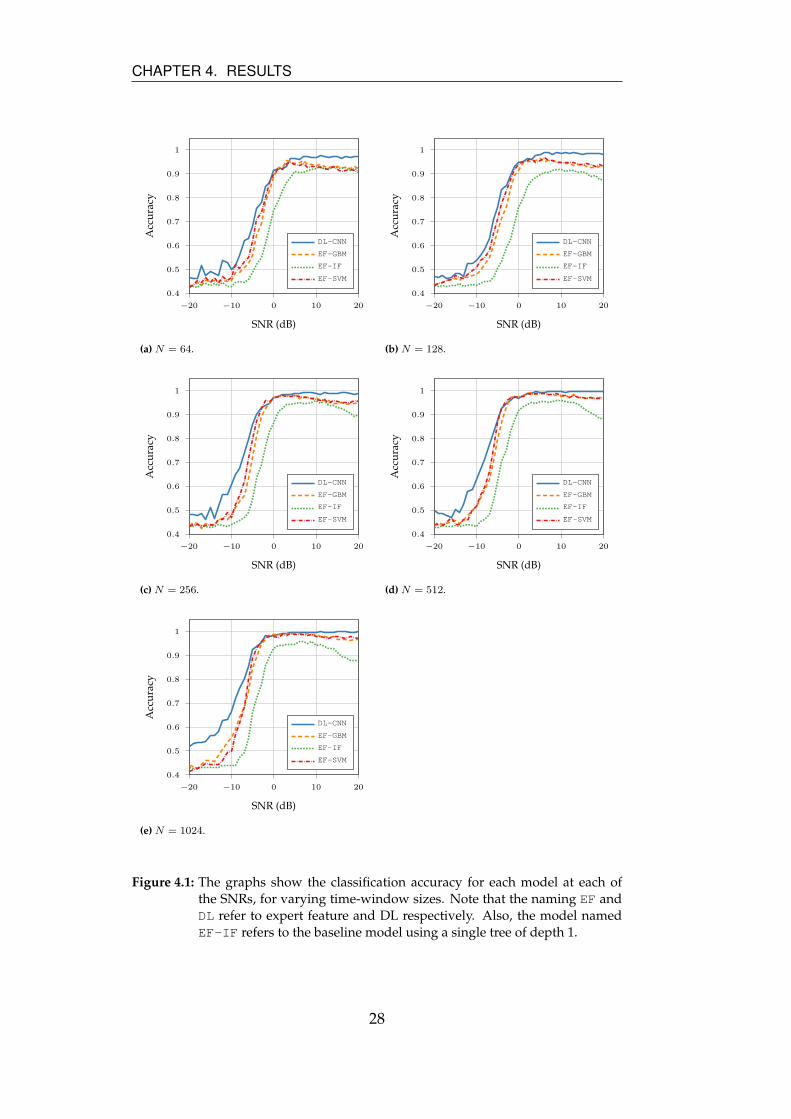
4.1 Accuracy comparison

Figure 4.1 allows for comparisons between the models in terms of ac-

curacy over a range of SNRs, at the different time-window sizes eval-

uated, as described in Section 3.3.1. It shows that the CNN model

outperforms the other models for SNRs below -5 and above 5 for all

time-window sizes.

27

CHAPTER 4. RESULTS

−20 −10 0 10 20

0.4

0.5

0.6

0.7

0.8

0.9

1

SNR (dB)

Acc

ura

cy

DL-CNN

EF-GBM

EF-IF

EF-SVM

(a) N = 64.

−20 −10 0 10 20

0.4

0.5

0.6

0.7

0.8

0.9

1

SNR (dB)

Acc

ura

cy

DL-CNN

EF-GBM

EF-IF

EF-SVM

(b) N = 128.

−20 −10 0 10 20

0.4

0.5

0.6

0.7

0.8

0.9

1

SNR (dB)

Acc

ura

cy

DL-CNN

EF-GBM

EF-IF

EF-SVM

(c) N = 256.

−20 −10 0 10 20

0.4

0.5

0.6

0.7

0.8

0.9

1

SNR (dB)

Acc

ura

cy

DL-CNN

EF-GBM

EF-IF

EF-SVM

(d) N = 512.

−20 −10 0 10 20

0.4

0.5

0.6

0.7

0.8

0.9

1

SNR (dB)

Acc

ura

cy

DL-CNN

EF-GBM

EF-IF

EF-SVM

(e) N = 1024.

Figure 4.1: The graphs show the classification accuracy for each model at each ofthe SNRs, for varying time-window sizes. Note that the naming EF andDL refer to expert feature and DL respectively. Also, the model namedEF-IF refers to the baseline model using a single tree of depth 1.

28

CHAPTER 4. RESULTS

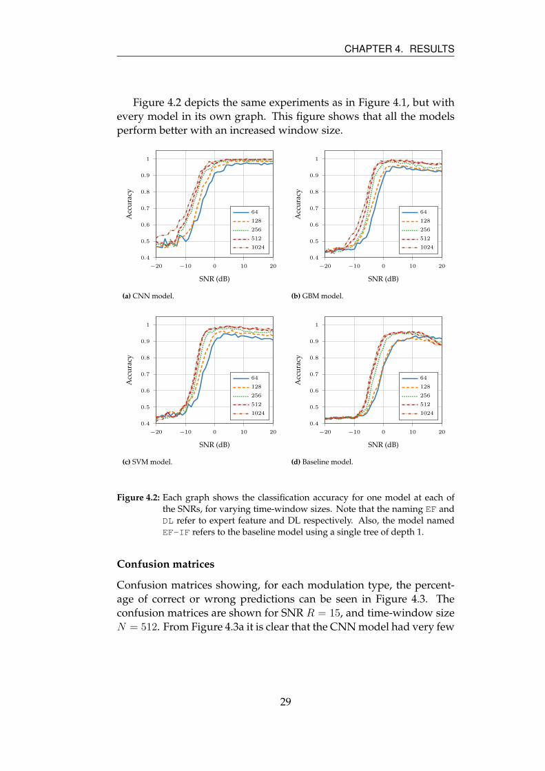
Figure 4.2 depicts the same experiments as in Figure 4.1, but with

every model in its own graph. This figure shows that all the models

perform better with an increased window size.

−20 −10 0 10 20

0.4

0.5

0.6

0.7

0.8

0.9

1

SNR (dB)

Acc

ura

cy

64

128

256

512

1024

(a) CNN model.

−20 −10 0 10 20

0.4

0.5

0.6

0.7

0.8

0.9

1

SNR (dB)

Acc

ura

cy

64

128

256

512

1024

(b) GBM model.

−20 −10 0 10 20

0.4

0.5

0.6

0.7

0.8

0.9

1

SNR (dB)

Acc

ura

cy

64

128

256

512

1024

(c) SVM model.

−20 −10 0 10 20

0.4

0.5

0.6

0.7

0.8

0.9

1

SNR (dB)

Acc

ura

cy

64

128

256

512

1024

(d) Baseline model.

Figure 4.2: Each graph shows the classification accuracy for one model at each ofthe SNRs, for varying time-window sizes. Note that the naming EF andDL refer to expert feature and DL respectively. Also, the model namedEF-IF refers to the baseline model using a single tree of depth 1.

Confusion matrices

Confusion matrices showing, for each modulation type, the percent-

age of correct or wrong predictions can be seen in Figure 4.3. The

confusion matrices are shown for SNR R = 15, and time-window size

N = 512. From Figure 4.3a it is clear that the CNN model had very few

29

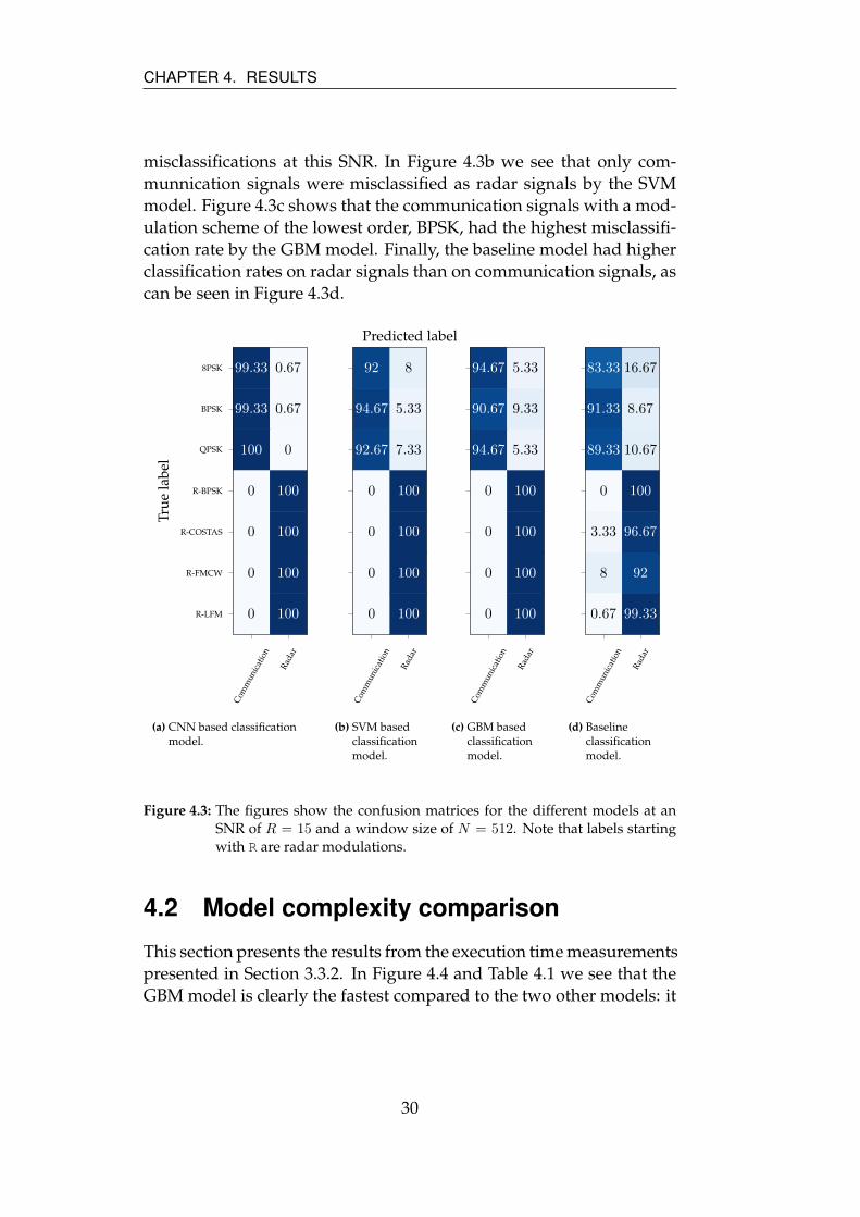
CHAPTER 4. RESULTS

misclassifications at this SNR. In Figure 4.3b we see that only com-

munnication signals were misclassified as radar signals by the SVM

model. Figure 4.3c shows that the communication signals with a mod-

ulation scheme of the lowest order, BPSK, had the highest misclassifi-

cation rate by the GBM model. Finally, the baseline model had higher

classification rates on radar signals than on communication signals, as

can be seen in Figure 4.3d.

Predicted label

Com

mu

nica

tion

Rad

ar

8PSK

BPSK

QPSK

R-BPSK

R-COSTAS

R-FMCW

R-LFM

99.33 0.67

99.33 0.67

100 0

0 100

0 100

0 100

0 100

Tru

ela

bel

(a) CNN based classificationmodel.

Com

mu

nica

tion

Rad

ar

92 8

94.67 5.33

92.67 7.33

0 100

0 100

0 100

0 100

(b) SVM basedclassificationmodel.

Com

mu

nica

tion

Rad

ar

94.67 5.33

90.67 9.33

94.67 5.33

0 100

0 100

0 100

0 100

(c) GBM basedclassificationmodel.

Com

mu

nica

tion

Rad

ar

83.33 16.67

91.33 8.67

89.33 10.67

0 100

3.33 96.67

8 92

0.67 99.33

(d) Baselineclassificationmodel.

Figure 4.3: The figures show the confusion matrices for the different models at anSNR of R = 15 and a window size of N = 512. Note that labels startingwith R are radar modulations.

4.2 Model complexity comparison

This section presents the results from the execution time measurements

presented in Section 3.3.2. In Figure 4.4 and Table 4.1 we see that the

GBM model is clearly the fastest compared to the two other models: it

30

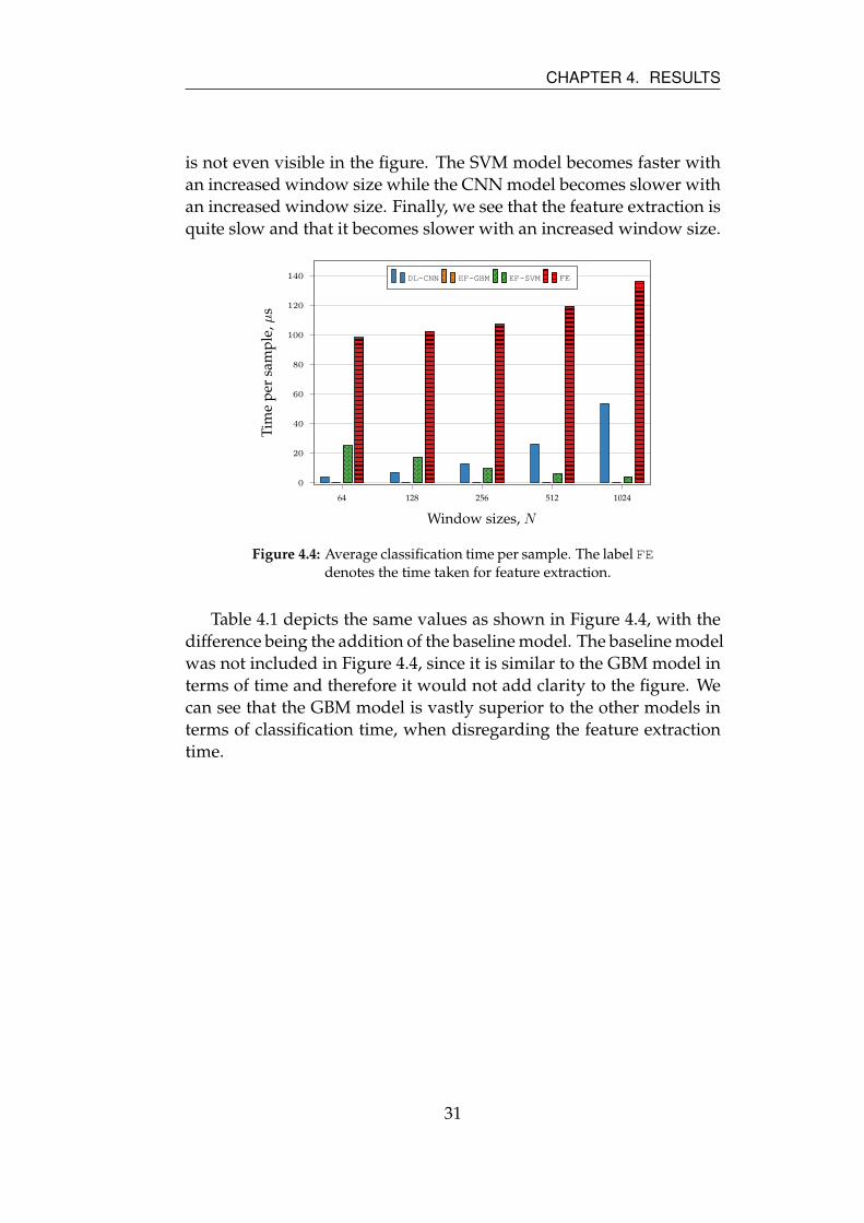
CHAPTER 4. RESULTS

is not even visible in the figure. The SVM model becomes faster with

an increased window size while the CNN model becomes slower with

an increased window size. Finally, we see that the feature extraction is

quite slow and that it becomes slower with an increased window size.

64 128 256 512 1024

0

20

40

60

80

100

120

140

Window sizes, N

Tim

ep

ersa

mp

le,µ

sDL-CNN EF-GBM EF-SVM FE

Figure 4.4: Average classification time per sample. The label FEdenotes the time taken for feature extraction.

Table 4.1 depicts the same values as shown in Figure 4.4, with the

difference being the addition of the baseline model. The baseline model

was not included in Figure 4.4, since it is similar to the GBM model in

terms of time and therefore it would not add clarity to the figure. We

can see that the GBM model is vastly superior to the other models in

terms of classification time, when disregarding the feature extraction

time.

31

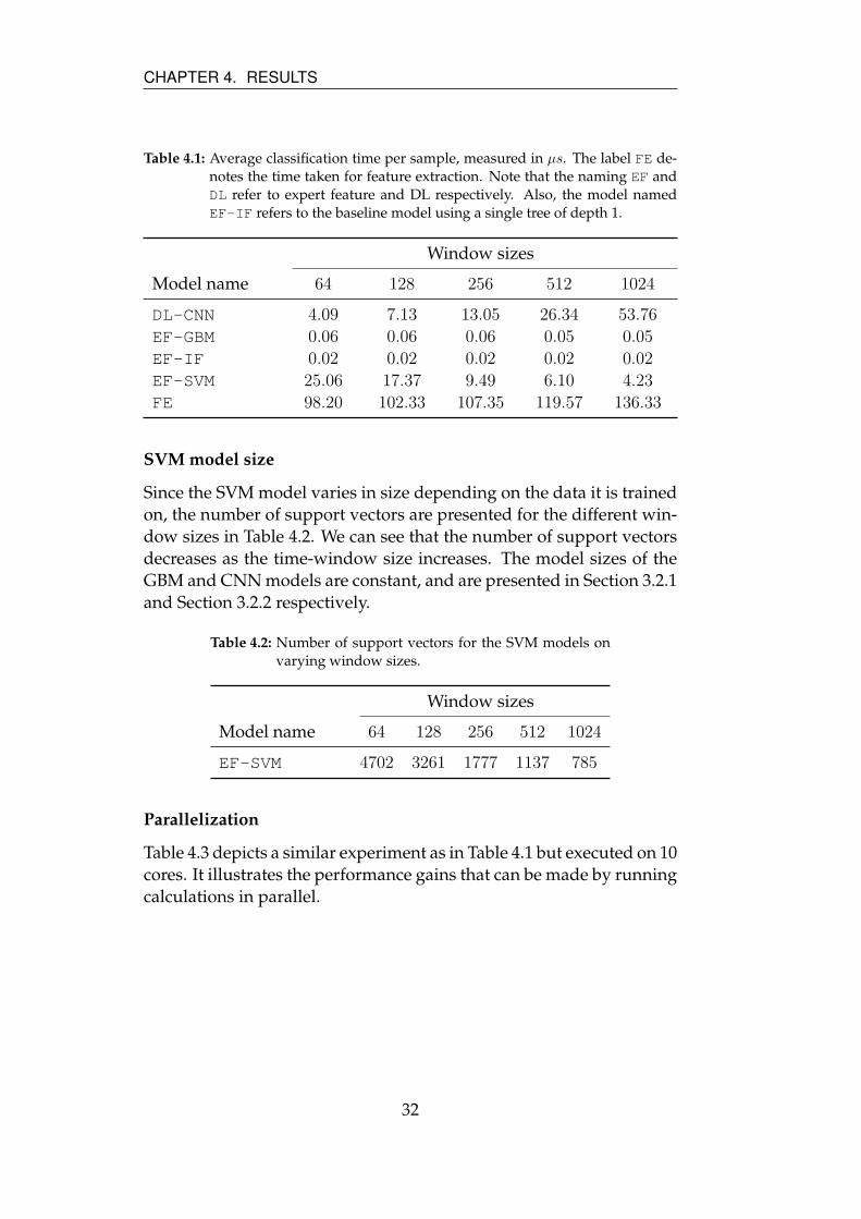
CHAPTER 4. RESULTS

Table 4.1: Average classification time per sample, measured in µs. The label FE de-notes the time taken for feature extraction. Note that the naming EF andDL refer to expert feature and DL respectively. Also, the model namedEF-IF refers to the baseline model using a single tree of depth 1.

Window sizes

Model name 64 128 256 512 1024

DL-CNN 4.09 7.13 13.05 26.34 53.76

EF-GBM 0.06 0.06 0.06 0.05 0.05

EF-IF 0.02 0.02 0.02 0.02 0.02

EF-SVM 25.06 17.37 9.49 6.10 4.23

FE 98.20 102.33 107.35 119.57 136.33

SVM model size

Since the SVM model varies in size depending on the data it is trained

on, the number of support vectors are presented for the different win-

dow sizes in Table 4.2. We can see that the number of support vectors

decreases as the time-window size increases. The model sizes of the

GBM and CNN models are constant, and are presented in Section 3.2.1

and Section 3.2.2 respectively.

Table 4.2: Number of support vectors for the SVM models onvarying window sizes.

Window sizes

Model name 64 128 256 512 1024

EF-SVM 4702 3261 1777 1137 785

Parallelization

Table 4.3 depicts a similar experiment as in Table 4.1 but executed on 10

cores. It illustrates the performance gains that can be made by running

calculations in parallel.

32

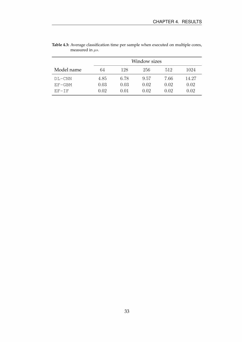
CHAPTER 4. RESULTS

Table 4.3: Average classification time per sample when executed on multiple cores,measured in µs.

Window sizes

Model name 64 128 256 512 1024

DL-CNN 4.85 6.78 9.57 7.66 14.27

EF-GBM 0.03 0.03 0.02 0.02 0.02

EF-IF 0.02 0.01 0.02 0.02 0.02

33

Chapter 5

Discussion

This chapter begins with a discussion of the results of the accuracy ex-

periment, followed by the execution time experiment. The final section

discusses the implications of the results in an RWR setting.

5.1 Accuracy comparison

The results from the accuracy experiment, presented in Figure 4.1, in-

dicate that the CNN model is the best at generalizing to unseen data

since the accuracy drops slower than for the other two models as the

SNR decreases. Also, it seems to be monotonically increasing with in-

creased SNR, meaning it achieves nearly a perfect score on the higher

SNRs. This differs from the other models, which decrease in accuracy

on data at SNRs above R = 10. As explained in Section 3.1.4 only SNRs

in the range [−5, 10] were present in the training data.

It could be argued that not including all SNRs in training makes for

an unfair comparison between the models, especially due to the nor-

malization that is performed for the expert feature based models. The

reason for this was to see how well the models performed on unseen

data. Also, higher SNRs make for data that should be easier to clas-

sify. It may be a more fair comparison to include modulation types in

the test set which were not present in the training set, for both com-

munication signals and radar signals, in order to see how the models

generalize on completely unseen data.

The GBM model seems to perform well on the SNR range used for

training. It sometimes beats the CNN model for SNRs near R = 0,

which can be seen in Figures 4.1c, 4.1d and 4.1e. However, it drops

34

CHAPTER 5. DISCUSSION

very fast in accuracy as the SNR decreases and it even drops a bit as

the SNR increases beyond R = 10, for all window sizes. This suggests

that this model is not as good at generalizing to unseen data as the

CNN model.

The SVM model has very similar performance compared to the

GBM model, with the same problem of performing worse as the SNR

increases beyond the ranges used for training, as seen in Figure 4.1.

This suggests that the difficulty in generalization lies in the approach,

and that it is based on expert features.

Finally, the baseline model, which is basically a simple if-statement,

still performs quite well. It achieves above 90% accuracy for SNRs

in the range [0, 10] for most window sizes. This shows the simplicity

of the problem at reasonable noise levels. The fact that the accuracy

drops as the SNR increases past the range used for training is further

evidence for the fact that the feature based approach has difficulty gen-

eralizing on unseen data.

Confusion matrices

From Figure 4.3 we can see that at an SNR of R = 15, the CNN model

performs best, and that the SVM model seems to mostly make mis-

takes predicting that a sample is a radar signal when it is actually a

communication signal. This could be due to the fact that the mod-

ulation of communication signals is similar to radar signals at lower

SNRs and that this affects the predictions at higher SNRs since the ac-

tual SNR is hidden to the model.

In Figure 4.3c we see that the GBM model seems to also misclas-

sify communication signals as radar signals and not vice versa. It also

seems like the BPSK modulation is mistaken more than the others.

The reason for this could be that in the lower degrees of modulation

the changes to the phase are quite large, as explained in Section 2.1.1,

which could make them similar to for example BPSK modulation in

radar signals.

5.2 Model complexity comparison

From Table 4.1 we can see that the classification time of the CNN

model seems to depend approximately linearly on the window size

N , meaning the slight gain in accuracy comes at a quite large cost in

35

CHAPTER 5. DISCUSSION

terms of computations. Therefore, it would be critical to weigh the

gained accuracy against this cost in computation time if this model

was to be implemented in an RWR.

The baseline model is easily the fastest, which is expected consid-

ering the size of the model being a single if-statement. The second

fastest is the GBM model, again as expected. It is important to remem-

ber that the time required for the feature extraction process does need

to be added to the classification time of the models based on expert fea-

tures. The time required for feature extraction, presented in Figure 4.4

and Table 4.1, is not representative of the time that can be achieved if

implemented for optimal execution time. The scaling, with the win-

dow size N , of the feature extraction is still relevant, which is why it

was included in the results.

In this thesis, the feature extraction was implemented in Python us-

ing NumPy for vector operations, as stated in Section 3.2.1. This results

in a large overhead for the system when calculating these features and

if it was to be implemented in an RWR it could be made much more

efficient. Some of the analog features used in this thesis are already

calculated and used for other purposes in many RWRs, meaning that

those would come at no additional cost.

As for the SVM model we see that the highest classification time

is recorded on the lowest window size, although it is still faster than

the slowest time of the CNN model when disregarding the feature ex-

traction. This is most probably due to the fact that as the window size

gets smaller the features used become more unstable, evidenced by

the lower accuracy of both expert feature-based models on decreased

window sizes as seen in Figures 4.2b and 4.2c. As the features be-

come more unstable the SVM model compensates by including more

support vectors to achieve a good result on the training set, which in

turn increases the computational complexity for classification. This is

further evidenced by Table 4.2 which displays the number of support

vectors used at each of the window sizes. Since the SVM model also

uses the features, the same arguments hold as for the GBM model.

Parallelization

As mentioned in Section 3.3.2, the measured times presented in Fig-

ure 4.4 are achieved when evaluating the models on a single core of

the CPU. All three of the models, however, could benefit greatly from

36

CHAPTER 5. DISCUSSION

running more calculations in parallel, as evidenced by Table 4.3.

In theory, it should be possible to calculate all the kernel evalua-

tions for the support vectors in the SVM model in parallel and then

simply sum the result, which would allow for a much shorter classi-

fication time. In the CNN model, a similar improvement in classifica-

tion time could be made by parallelizing each layer of the model. The

depth of the network would, in this case, be a limiting factor for par-

allelizing since the result of the previous layer must be known before

being able to calculate the next layer. Thus, deeper networks mean

slower classification times when fully parallelized. The fact that the

classification time for window size N = 64 barely changed despite

being executed on 10 CPU cores instead of 1 supports this claim. As

for the GBM model, it is similar to the CNN model since the depth of

the trees are the limiting factor for parallelization, as each tree in the

model can be evaluated individually.

5.3 Radar warning receiver setting

As mentioned in Chapter 1, the RWR setting introduces many limita-

tions on the classification model. The model size is one of the primary

limitations, i.e., the absolute size of the model and how it could be

implemented in a system, either in software or in some kind of pro-

grammable hardware. To this requirement, the GBM and CNN mod-

els have an advantage compared to the SVM model, since they can be

designed with a specific size constraint in mind and then trained on

as much data as possible to achieve good performance in terms of ac-

curacy. The CNN model is considerably larger than the GBM model,

meaning the increased performance comes at a large cost in terms of

model size. For the SVM, the model size depends on the variance of

the data that is used, as discussed in Section 5.2.

As mentioned in Section 3.1 the stage at which IQ data is available

is basically the first step in the signal processing chain. This means

there needs to be a high throughput of signals. Therefore, the time al-

lowed for classification is another primary limitation, which is closely

tied to the model size and the same arguments for the CNN and GBM

models still hold. The CNN model can gain performance in terms of

classification time if parallelized further, as evidenced by Table 4.3.

This makes the actual model size a stronger limitation in an RWR.

37

CHAPTER 5. DISCUSSION

The advantage of performing the filtering at this stage, is that the

signals are visually very different at this point for reasonable SNRs,

which should allow for a very simple and fast model to perform the

classifications, as evidenced by the if-statement baseline performing

above 90% for SNRs in the range [0, 10].

Although the results show that simple classification models using

expert features do not generalize very well on unseen data, this should

not be used as an argument to rule them out completely. Consider-

ing the fact that radar signals and communication signals are quite

well-defined in terms of their analytic representations, a reasonable

assumption is that most of the samples that appear in a real-world

scenario have already been seen during training and should therefore

be classified correctly. This places more importance on collecting data

that is realistic and covers the samples that appear in a real-world sce-

nario.

Flexibility

The main difference between a DL approach for classification, such as

the CNN model presented in this thesis, and an approach based on ex-

pert features is in terms of flexibility. For example, a new radar modu-

lation type could be introduced which renders the features chosen for

the classifier unsuitable. In this case, a model based on expert features

would potentially require quite a large change in the RWR depending

on how the feature extraction is implemented. For a DL model, on the

contrary, a simple re-training of the model with the new modulation

type would suffice to capture this new modulation type.

Furthermore, a DL model could easily be extended in order to fill

several purposes with the same input. For example, if it is of interest

to classify between radar modulation types, extending the network to

allow for this is rather simple in a DL model, at the cost of a more

complex network. For the approach based on expert features, on the

other hand, it is likely that new features specifically designed for the

new purpose would have to be introduced making this change involve

more work to take it from idea to implementation.

38

Chapter 6

Conclusions

In conclusion the CNN model using the DL approach outperforms

the models based on expert features in terms of accuracy, as has been

clearly evidenced in multiple other fields. Furthermore, this type of

model seems to be better at generalizing on completely unseen data,

which is also of great importance in an RWR.

However, in an RWR setting the time constraint is quite significant

and in this regard the GBM model is vastly superior with only a slight

decrease in accuracy, assuming the feature extraction is implemented

more efficiently than in this thesis. Although the results in this thesis

indicate that the GBM model is worse than the CNN model at gener-

alizing on unseen data, this is probably not a prohibiting factor con-

sidering how well-defined communication signals and radar signals

are in their analytic representation. It does increase the importance of

collecting enough realistic data to use for training the model.

Thus, both approaches have their strengths and if this type of filter

was to be implemented in an RWR the performance in accuracy will

have to be weighed against the model size and classification time.

Considering their flexibility and extendability, CNN models are

probably better suited for more complex tasks. It would be interesting

to investigate if a couple of different tasks in an RWR could be solved

simultaneously using a DL approach. In this case, filtering communi-

cation signals could be one of the tasks to be included.

Future work should focus on optimizing the feature extraction

process, in order to achieve a fair comparison in terms of classification

time for the different models. Evaluating the models on recorded data

could change the results, which is also left for future work.

39

Bibliography

[1] M. Abadi et al. TensorFlow: Large-Scale Machine Learning on

Heterogeneous Systems. Software available from tensorflow.org.

2015. URL: https://www.tensorflow.org/.

[2] A. Abdelmutalab, K. Assaleh, and M. El-Tarhuni. “Automatic

modulation classification based on high order cumulants and

hierarchical polynomial classifiers”. In: Physical Communication

21 (2016), pp. 10–18.

[3] About GNU Radio. 2018. URL:

https://www.gnuradio.org/about/ (visited on 05/04/2018).

[4] K. S. K. Arumugam et al. “Modulation recognition using side

information and hybrid learning”. In: 2017 IEEE International

Symposium on Dynamic Spectrum Access Networks (DySPAN).

IEEE. 2017, pp. 1–2.

[5] C. M. Bishop. Pattern Recognition and Machine Learning.

Springer, 2006.

[6] D. Boudreau et al. “A fast automatic modulation recognition

algorithm and its implementation in a spectrum monitoring

application”. In: Proceedings of the 21st Century Military

Communications Conference (MILCOM 2000). Vol. 2. IEEE. 2000,

pp. 732–736.

[7] T. Chen and C. Guestrin. “XGBoost: A scalable tree boosting

system”. In: Proceedings of the 22nd ACM SIGKDD International

Conference on Knowledge Discovery and Data Mining. ACM. 2016,

pp. 785–794.

[8] H.-I. Choi and W. J. Williams. “Improved time-frequency

representation of multicomponent signals using exponential

kernels”. In: IEEE Transactions on Acoustics, Speech, and Signal

Processing 37.6 (1989), pp. 862–871.

40

BIBLIOGRAPHY

[9] F. Chollet et al. Keras. https://keras.io. 2015.

[10] O. A. Dobre, Y. Bar-Ness, and W. Su. “Higher-order cyclic

cumulants for high order modulation classification”. In:

Military Communications Conference (MILCOM 2003). Vol. 1.

IEEE. 2003, pp. 112–117.

[11] J. M. Giron-Sierra. Digital Signal Processing with Matlab Examples.

Vol. 1. Springer, 2017.

[12] S. W. Golomb and H. Taylor. “Constructions and properties of

Costas arrays”. In: Proceedings of the IEEE 72.9 (1984),

pp. 1143–1163.

[13] I. Goodfellow, Y. Bengio, and A. Courville. Deep Learning. MIT

Press, 2016. URL: http://www.deeplearningbook.org.

[14] E. Gopi. Digital Signal Processing for Wireless Communication

Using Matlab. Springer, 2016. DOI: 10.1007/978-3-319-20651-6.

[15] K. He et al. “Deep residual learning for image recognition”. In:

Proceedings of the IEEE Conference on Computer Vision and Pattern

Recognition. 2016, pp. 770–778.

[16] D. H. Johnson. “Signal-to-noise ratio”. In: Scholarpedia 1.12

(2006). revision #91770, p. 2088. DOI: 10.4249/scholarpedia.2088.

[17] M. I. Jordan and T. M. Mitchell. “Machine learning: Trends,

perspectives, and prospects”. In: Science 349.6245 (2015),

pp. 255–260. ISSN: 0036-8075. DOI: 10.1126/science.aaa8415.

[18] D. P. Kingma and J. Ba. “Adam: A method for stochastic

optimization”. In: arXiv preprint arXiv:1412.6980 (2014).

[19] S. Kokoska and D. Zwillinger. CRC Standard Probability and

Statistics Tables and Formulae. CRC Press, 1999.

[20] S.-H. Kong et al. “Automatic LPI radar waveform recognition

using CNN”. In: IEEE Access 6 (2018), pp. 4207–4219.

[21] N. Levanon and E. Mozeson. Radar Signals. John Wiley & Sons,

2004.

[22] J. Lundén and V. Koivunen. “Automatic radar waveform

recognition”. In: IEEE Journal of Selected Topics in Signal

Processing 1.1 (2007), pp. 124–136.

[23] S. Marsland. Machine Learning: An Algorithmic Perspective. CRC

Press, 2015.

41

BIBLIOGRAPHY

[24] A. K. Nandi and E. E. Azzouz. “Algorithms for automatic

modulation recognition of communication signals”. In: IEEE

Transactions on Communications 46.4 (1998), pp. 431–436.

[25] T. E. Oliphant. A guide to NumPy. Vol. 1. Trelgol Publishing

USA, 2006.

[26] T. J. O’Shea and N. West. “Radio machine learning dataset

generation with GNU radio”. In: Proceedings of the GNU Radio

Conference. Vol. 1. 1. 2016.

[27] T. J. O’Shea, T. Roy, and T. C. Clancy. “Over-the-air deep

learning based radio signal classification”. In: IEEE Journal of

Selected Topics in Signal Processing 12.1 (2018), pp. 168–179.

[28] Y. Park and F. Adachi. Enhanced Radio Access Technologies for

Next Generation Mobile Communication. Springer, 2007.

[29] F. Pedregosa et al. “Scikit-learn: Machine learning in Python”.

In: Journal of Machine Learning Research 12 (2011), pp. 2825–2830.

[30] M. Petrova, P. Mähönen, and A. Osuna. “Multi-class

classification of analog and digital signals in cognitive radios

using Support Vector Machines”. In: 2010 7th International

Symposium on Wireless Communication Systems (ISWCS). IEEE.

2010, pp. 986–990. DOI: 10.1109/ISWCS.2010.5624500.

[31] J. R. Quinlan. C4.5: Programs for Machine Learning. Morgan

Kaufmann, 1993.

[32] S. Wunsch. GNU Radio Radar Toolbox. 2018. URL:

https://grradar.wordpress.com/info/ (visited on 05/04/2018).

[33] T. Yucek and H. Arslan. “A survey of spectrum sensing

algorithms for cognitive radio applications”. In: IEEE

Communications Surveys & Tutorials 11.1 (2009), pp. 116–130.

42