Embed Size (px)
Citation preview
SIAM J. COMPUT. c© 2006 Society for Industrial and Applied MathematicsVol. 36, No. 1, pp. 132–157
FAST MONTE CARLO ALGORITHMS FOR MATRICES I:APPROXIMATING MATRIX MULTIPLICATION∗
PETROS DRINEAS† , RAVI KANNAN‡ , AND MICHAEL W. MAHONEY§
Abstract. Motivated by applications in which the data may be formulated as a matrix, weconsider algorithms for several common linear algebra problems. These algorithms make more effi-cient use of computational resources, such as the computation time, random access memory (RAM),and the number of passes over the data, than do previously known algorithms for these problems.In this paper, we devise two algorithms for the matrix multiplication problem. Suppose A and B(which are m × n and n × p, respectively) are the two input matrices. In our main algorithm, weperform c independent trials, where in each trial we randomly sample an element of {1, 2, . . . , n} withan appropriate probability distribution P on {1, 2, . . . , n}. We form an m × c matrix C consistingof the sampled columns of A, each scaled appropriately, and we form a c × n matrix R using thecorresponding rows of B, again scaled appropriately. The choice of P and the column and row scalingare crucial features of the algorithm. When these are chosen judiciously, we show that CR is a goodapproximation to AB. More precisely, we show that
‖AB − CR‖F = O(‖A‖F ‖B‖F /√c),
where ‖·‖F denotes the Frobenius norm, i.e., ‖A‖2F =
∑i,j
A2ij . This algorithm can be implemented
without storing the matrices A and B in RAM, provided it can make two passes over the matricesstored in external memory and use O(c(m+n+p)) additional RAM to construct C and R. We thenpresent a second matrix multiplication algorithm which is similar in spirit to our main algorithm.In addition, we present a model (the pass-efficient model) in which the efficiency of these and otherapproximate matrix algorithms may be studied and which we argue is well suited to many applicationsinvolving massive data sets. In this model, the scarce computational resources are the number ofpasses over the data and the additional space and time required by the algorithm. The input matricesmay be presented in any order of the entries (and not just row or column order), as is the case inmany applications where, e.g., the data has been written in by multiple agents. In addition, the inputmatrices may be presented in a sparse representation, where only the nonzero entries are written.
Key words. randomized algorithms, Monte Carlo methods, massive data sets, streaming mod-els, matrix multiplication
AMS subject classification. 68W20
DOI. 10.1137/S0097539704442684
1. Introduction. We are interested in developing and analyzing fast MonteCarlo algorithms for performing useful computations on large matrices. Examplesof such computations include matrix multiplication, the computation of the singularvalue decomposition of a matrix, and the computation of compressed approximatedecompositions of a matrix. In this paper, we present a computational model forcomputing on massive data sets (the pass-efficient model) in which our algorithms
∗Received by the editors April 5, 2004; accepted for publication (in revised form) November 17,2005; published electronically May 26, 2006. The technical report version of this paper appeared asFast Monte Carlo Algorithms for Matrices I: Approximating Matrix Multiplication, by P. Drineas,R. Kannan, and M. W. Mahoney [13]. A preliminary version of this paper, including the mainalgorithm and main theorem of section 4, appeared as Fast Monte-Carlo algorithms for approximatematrix multiplication, by P. Drineas and R. Kannan, in Proceedings of the 42nd Annual Symposiumon Foundations of Computer Science, 2001, pp. 452–459.
http://www.siam.org/journals/sicomp/36-1/44268.html†Department of Computer Science, Rensselaer Polytechnic Institute, Troy, NY 12180 (drinep@cs.
rpi.edu).‡Department of Computer Science, Yale University, New Haven, CT 06520 ([email protected]).
This author was supported in part by a grant from the NSF.§Department of Mathematics, Yale University, New Haven, CT 06520 ([email protected]).
132
FAST MONTE CARLO ALGORITHMS FOR MATRICES I 133
may naturally be formulated; we also present two algorithms for the approximationof the product of two matrices. In a second paper we present two algorithms for thecomputation of low-rank approximations to a matrix [11]. Finally, in a third paperwe present two algorithms to compute a compressed approximate decomposition toa matrix that has several appealing properties [12]. We expect our algorithms tobe useful in many applications where data sets are modeled by matrices and areextremely large. For example, in information retrieval and data mining (two rapidlygrowing areas of research in computer science and scientific computation that buildon techniques and theories from fields such as statistics, linear algebra, databasetheory, pattern recognition, and learning theory) a large collection of m objects, e.g.,documents, genomes, images, or web pages, is implicitly presented as a set of pointsin an n-dimensional Euclidean space, where n is the number of features that describethe object. This collection may be represented by an m × n matrix A, the rows ofwhich are the object vectors and the columns of which are the feature vectors.
Recent interest in computing with massive data sets has led to the development ofcomputational models in which the usual notions of time efficiency and space efficiencyhave been modified [23, 19, 3, 14, 10, 5]. In the applications that motivate these data-streaming models [19, 5], e.g., the observational sciences and the monitoring andoperation of large networked systems, the data sets are much too large to fit intomain memory. Thus, they are either not stored or are stored in a secondary storagedevice which may be read sequentially as a data stream but for which random accessis very expensive. Typically, algorithms that compute on a data stream examine thedata stream, keep a small “sketch” of the data, and perform computations on thesketch. Thus, these algorithms are usually randomized and approximate, and theirperformance is evaluated by considering resources such as the time to process an itemin the data stream, the number of passes over the data, the additional workspace andadditional time required, and the quality of the approximations returned. (Note thatin some cases the term “data-streaming model” refers to a model in which only asingle pass over the data is allowed [19, 5].)
The motivation for our particular “pass-efficient” approach is that in moderncomputers the amount of external memory (e.g., disk storage or tape storage) hasincreased enormously, while RAM and computing speeds have increased, but at asubstantially slower pace. Thus, we have the ability to store large amounts of data,but not in RAM, and we do not have the computational ability to process these datawith algorithms that require superlinear time. A related motivation is that input-output rates have not increased proportionally. Thus, the size of the data inputs (aslimited, e.g., by the size of disks) has increased substantially faster than the rate atwhich we can access the data randomly.
In order to provide a framework in which to view the algorithms presented herein,we first introduce and describe the pass-efficient model of data-streaming computa-tion [10]. In the pass-efficient model the computational resources are the numberof sequential-access passes over the data and the additional RAM space and theadditional time required. Thus, our algorithms are quite different from traditionalnumerical analysis approaches and generally fit within the following framework. Ouralgorithms will be allowed to read the matrices from external storage a few—e.g., oneor two or three—times and keep a small randomly chosen and rapidly computable“sketch” of the matrices in RAM. Our algorithms will also be permitted additionalRAM space and additional time in order to perform computations on the “sketch.”The results of these computations will be returned as approximations to the solutionof the original problem.
134 PETROS DRINEAS, RAVI KANNAN, AND MICHAEL W. MAHONEY
In all of our algorithms, an important implementation issue will be how to formthe random sample. An obvious choice is to use uniform sampling, where each dataobject is equally likely to be picked. Uniform sampling can be performed blindly, inwhich case the sample to be chosen can be decided before seeing the data. Even whenthe number of data elements is not known in advance an element can be selecteduniformly at random in one pass over the data; see Lemma 1. Uniform sampling fitswithin our framework and is useful for certain (restricted) classes of problems. Toobtain much more generality, we will sample according to a judiciously chosen (anddata-dependent) set of nonuniform sampling probabilities. This nonuniform sampling,in which in the first pass through the data we compute sampling probabilities (e.g.,we may keep rows or columns of a data matrix with probability proportional to thesquare of their lengths) and in the second pass we draw the sample, offers substantialgains. For example, it allows us to approximately solve problems in sparse matricesas well as dense matrices.
The idea of sampling rows or columns of matrices in order to approximate variousoperations is not new; indeed, a motivation for our main matrix multiplication algo-rithm came from [15]. In this paper and accompanying work [11, 12], we extend thoseideas and develop algorithms with provable error bounds for a variety of matrix oper-ations. One of the main contributions of our work is to demonstrate that a “sketch”consisting of a small judiciously chosen random sample of rows and/or columns of theinput matrix or matrices is adequate for provably rapid and efficient approximation ofseveral common matrix operations. We believe that the underlying principle of usingnonuniform sampling to create “sketches” of the data in a small number of passes(and “pass-efficient” approaches more generally) constitutes an appealing and fruitfuldirection for algorithmic research in order to address the size and nature of moderndata sets.
In the present paper, we present two simple and intuitive algorithms which, whengiven an m× n matrix A and an n× p matrix B, compute an approximation to theproduct AB. In the first algorithm, the BasicMatrixMultiplication algorithm ofsection 4, we perform c independent trials, where in each trial we randomly sample anelement of {1, 2, . . . , n} with an appropriate probability distribution P on {1, 2, . . . , n}.We form an m × c matrix C consisting of the sampled columns of A, each scaledappropriately, and we form a c×n matrix R using the corresponding rows of B, againscaled appropriately. The choice of P and the column and row scaling are crucialfeatures of the algorithm. When these are chosen judiciously, we show that CR is agood approximation to AB. More precisely, we show that
‖AB − CR‖F = O( ‖A‖F ‖B‖F /√c),
where ‖·‖F denotes the Frobenius norm, i.e., ‖A‖2F =
∑i,j A
2ij , holds in expectation
and with high probability. Thus, in particular, when B = AT we have that if c =Ω(1/ε2), then ‖AAT −CCT ‖F ≤ ε ‖A‖2
F holds with high probability. This algorithmcan be implemented without storing the matrices A and B in RAM, provided it canmake two passes over the matrices stored in external memory and use O(c(m+n+p))additional RAM; thus it will be efficient in the pass-efficient model.
In the second algorithm, the ElementwiseMatrixMultiplication algorithmof section 5, which is an extension of ideas from [2, 1], elements of A and B, ratherthan columns and rows, are randomly either zeroed out or kept and rescaled, therebyconstructing matrices A and B. Although this algorithm lacks a useful bound on
FAST MONTE CARLO ALGORITHMS FOR MATRICES I 135
‖AB − AB‖F , under appropriate assumptions a bound on the spectral norm of theform
‖AB − AB‖2 = O( ‖A‖F ‖B‖F /√c)
holds with high probability.After this introduction, we provide in section 2 a review of the relevant linear
algebra, and in section 3 we introduce the pass-efficient model of data-streaming com-putation and discuss several technical sampling lemmas. In section 4 we introduceand analyze in detail the BasicMatrixMultiplication algorithm to approximatethe product of two matrices. Then, in section 5 we describe and analyze the Ele-
mentwiseMatrixMultiplication algorithm which is based on the ideas of [2, 1].Finally, in section 6 we provide a discussion and conclusion. In the appendix, weprovide further analysis of the BasicMatrixMultiplication algorithm.
2. Review of linear algebra. This section contains a review of some linearalgebra that will be useful throughout the paper. For more detail, see [18, 20, 25, 6]and the references therein.
For a vector x ∈ Rn we let |x| =
(∑ni=1 |xi|2
)1/2denote its Euclidean length.
For a matrix A ∈ Rm×n we let A(j), j = 1, . . . , n, denote the jth column of A as a
column vector and A(i), i = 1, . . . ,m, denote the ith row of A as a row vector. Wedenote matrix norms by ‖A‖ξ, using subscripts to distinguish between various norms.Of particular interest will be the Frobenius norm which is defined by
‖A‖F =
√√√√ m∑i=1
n∑j=1
A2ij ,(1)
and the spectral norm which is defined by
‖A‖2 = supx∈Rn, x �=0
|Ax||x| .(2)
These norms are related to each other as ‖A‖2 ≤ ‖A‖F ≤√n ‖A‖2.
3. The pass-efficient model and sampling lemmas. In this section, weinformally define a computational model in which the computational resources arethe number of passes over the data and the additional space and additional timerequired. In addition, we present several technical sampling lemmas.
3.1. The pass-efficient model. The pass-efficient model of data-streamingcomputation is a model that is motivated by the observation that in modern com-puters the amount of disk storage, i.e., sequential access memory, has increased veryrapidly while random access memory (RAM) and computing speeds have increased ata substantially slower pace [10]. Thus, one has the ability to store very large amountsof data but does not have random access to the data. Additionally, processing thedata with algorithms that take low polynomial time or linear time with large constantsis prohibitive.
To model this phenomenon, we consider the pass-efficient model, in which thethree computational resources of interest are the number of passes over the data andthe additional space and time required [10]. The data are assumed to be stored in anexternal disk space, to consist of elements whose size is bounded by a constant, and tobe presented to an algorithm on a read-only tape. The only access an algorithm has
136 PETROS DRINEAS, RAVI KANNAN, AND MICHAEL W. MAHONEY
to the data is via a pass, where a pass over the data is a sequential read of the entireinput from disk where only a constant amount of processing time is permitted per bitread. Note that this is a more restrictive notion of a pass over the data than in otherdata-streaming models [23, 19, 14]; in particular, in the pass-efficient model only aconstant rather than a logarithmic (in the data input length) amount of computationis permitted per bit read. In addition to the external disk space to store the dataand to a small number of passes over the data, an algorithm in the pass-efficientmodel is permitted to use additional RAM space and additional computation time.An algorithm operating in this model is considered pass-efficient if it requires a fixednumber of passes, independent of the input size, and additional space and time whichare sublinear in the length of the data stream in order to compute a “description” ofthe solution, which is then returned by the algorithm. A description of the solutionis either an explicit solution (if that is possible within the specified additional spaceand time) or an implicit representation of the solution that can be computed in theallotted additional space and time, and that can be expanded into an explicit solutionwith the additional expense of one pass over the data and linear (in the data inputlength) additional space and time. Note that, depending on the application, this laststep may or may not be necessary. Note also that if the data are represented byan m × n matrix, then the data stream has length O(mn) and an algorithm whichuses additional space and time that is linear in the number of data points or in thedimensionality of the data points, i.e., that is O(m) or O(n), is sublinear in the lengthof the data stream and thus is pass-efficient. We will be primarily interested in modelsthat require additional space and time that is either O(m+n) or constant with respectto m and n.
The sparse-unordered representation of data is a form of data representation inwhich each element of the data stream consists of a pair ((i, j), Aij) where the elementsin the data stream may be unordered with respect to the indices (i, j), and only thenonzero elements of the matrix A need to be presented. This very general form issuited to applications where, e.g., multiple agents may write parts of a matrix to acentral database and where one cannot make assumptions about the rules for write-conflict resolution. The data stream read by algorithms in the pass-efficient modelis assumed to be presented in the sparse-unordered representation. Other relatedmethods of data representation have been studied within the data-streaming context;see, e.g., [17] for applications to the problem of dynamic histogram maintenance.
3.2. Sampling lemmas. In this section we present two sampling primitives thatwill be used by our algorithms. Consider the Select algorithm presented in Figure 1.The following lemma establishes that in one pass over the data one can sample anelement according to certain probability distributions.
Lemma 1. Suppose that {a1, . . . , an}, ai ≥ 0, are read in one pass, i.e., onesequential read over the data, by the Select algorithm. Then the Select algorithmrequires O(1), i.e., constant with respect to n, additional storage space and returns arandom i∗ sampled from the probability distribution Pr [i∗ = i] = ai/
∑ni′=1 ai′ .
Proof. First, note that retaining the selected value and the running sum requiresO(1) additional space. The remainder of the proof is by induction. After reading
the first element a1, i∗ = 1 with probability a1/a1 = 1. Let D� =∑�
i′=1 ai′ andsuppose that the algorithm has read a1, . . . , a� thus far and has retained the runningsum D� and a sample i∗ such that Pr [i∗ = i] = ai/D�. Upon reading a�+1 thealgorithm lets i∗ = � + 1 with probability a�+1/D�+1 and retains i∗ at its previousvalue otherwise. At that point, clearly Pr [i∗ = � + 1] = a�+1/D�+1; furthermore for
FAST MONTE CARLO ALGORITHMS FOR MATRICES I 137
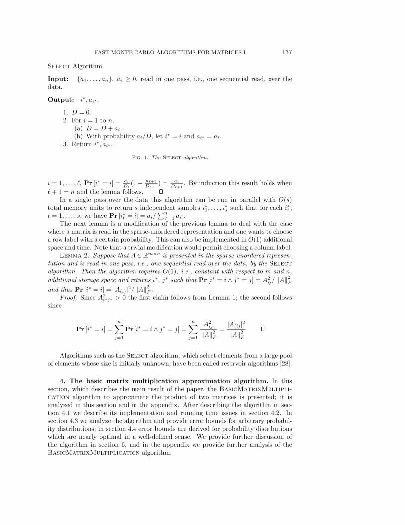
Select Algorithm.
Input: {a1, . . . , an}, ai ≥ 0, read in one pass, i.e., one sequential read, over thedata.
Output: i∗, ai∗ .
1. D = 0.2. For i = 1 to n,
(a) D = D + ai.(b) With probability ai/D, let i∗ = i and ai∗ = ai.
3. Return i∗, ai∗ .
Fig. 1. The Select algorithm.
i = 1, . . . , �, Pr [i∗ = i] = ai
D�(1 − a�+1
D�+1) = ai
D�+1. By induction this result holds when
� + 1 = n and the lemma follows.In a single pass over the data this algorithm can be run in parallel with O(s)
total memory units to return s independent samples i∗1, . . . , i∗s such that for each i∗t ,
t = 1, . . . , s, we have Pr [i∗t = i] = ai/∑n
i′=1 ai′ .The next lemma is a modification of the previous lemma to deal with the case
where a matrix is read in the sparse-unordered representation and one wants to choosea row label with a certain probability. This can also be implemented in O(1) additionalspace and time. Note that a trivial modification would permit choosing a column label.
Lemma 2. Suppose that A ∈ Rm×n is presented in the sparse-unordered represen-
tation and is read in one pass, i.e., one sequential read over the data, by the Select
algorithm. Then the algorithm requires O(1), i.e., constant with respect to m and n,
additional storage space and returns i∗, j∗ such that Pr [i∗ = i ∧ j∗ = j] = A2ij/ ‖A‖2
F
and thus Pr [i∗ = i] = |A(i)|2/ ‖A‖2F .
Proof. Since A2i∗j∗ > 0 the first claim follows from Lemma 1; the second follows
since
Pr [i∗ = i] =
n∑j=1
Pr [i∗ = i ∧ j∗ = j] =
n∑j=1
A2ij
‖A‖2F
=|A(i)|2
‖A‖2F
.
Algorithms such as the Select algorithm, which select elements from a large poolof elements whose size is initially unknown, have been called reservoir algorithms [28].
4. The basic matrix multiplication approximation algorithm. In thissection, which describes the main result of the paper, the BasicMatrixMultipli-
cation algorithm to approximate the product of two matrices is presented; it isanalyzed in this section and in the appendix. After describing the algorithm in sec-tion 4.1 we describe its implementation and running time issues in section 4.2. Insection 4.3 we analyze the algorithm and provide error bounds for arbitrary probabil-ity distributions; in section 4.4 error bounds are derived for probability distributionswhich are nearly optimal in a well-defined sense. We provide further discussion ofthe algorithm in section 6, and in the appendix we provide further analysis of theBasicMatrixMultiplication algorithm.
138 PETROS DRINEAS, RAVI KANNAN, AND MICHAEL W. MAHONEY
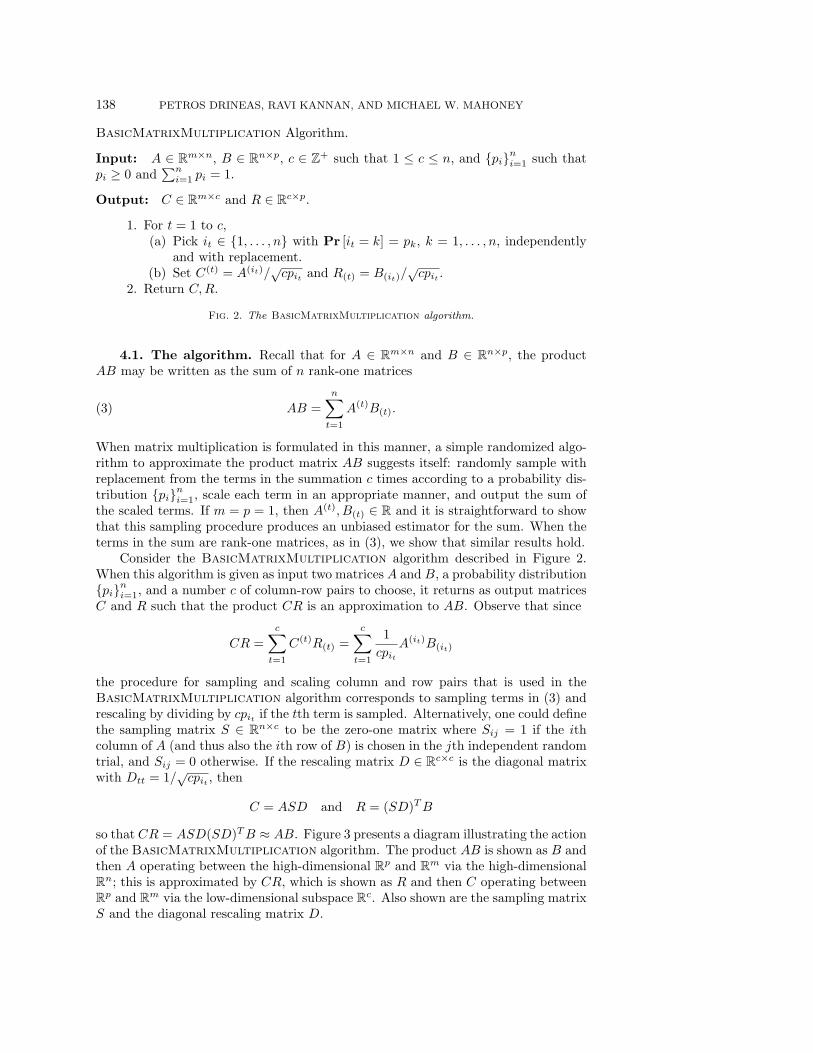
BasicMatrixMultiplication Algorithm.
Input: A ∈ Rm×n, B ∈ R
n×p, c ∈ Z+ such that 1 ≤ c ≤ n, and {pi}ni=1 such that
pi ≥ 0 and∑n
i=1 pi = 1.
Output: C ∈ Rm×c and R ∈ R
c×p.
1. For t = 1 to c,(a) Pick it ∈ {1, . . . , n} with Pr [it = k] = pk, k = 1, . . . , n, independently
and with replacement.(b) Set C(t) = A(it)/
√cpit and R(t) = B(it)/
√cpit .
2. Return C,R.
Fig. 2. The BasicMatrixMultiplication algorithm.
4.1. The algorithm. Recall that for A ∈ Rm×n and B ∈ R
n×p, the productAB may be written as the sum of n rank-one matrices
AB =
n∑t=1
A(t)B(t).(3)
When matrix multiplication is formulated in this manner, a simple randomized algo-rithm to approximate the product matrix AB suggests itself: randomly sample withreplacement from the terms in the summation c times according to a probability dis-tribution {pi}ni=1, scale each term in an appropriate manner, and output the sum ofthe scaled terms. If m = p = 1, then A(t), B(t) ∈ R and it is straightforward to showthat this sampling procedure produces an unbiased estimator for the sum. When theterms in the sum are rank-one matrices, as in (3), we show that similar results hold.
Consider the BasicMatrixMultiplication algorithm described in Figure 2.When this algorithm is given as input two matrices A and B, a probability distribution{pi}ni=1, and a number c of column-row pairs to choose, it returns as output matricesC and R such that the product CR is an approximation to AB. Observe that since
CR =
c∑t=1
C(t)R(t) =
c∑t=1
1
cpitA(it)B(it)
the procedure for sampling and scaling column and row pairs that is used in theBasicMatrixMultiplication algorithm corresponds to sampling terms in (3) andrescaling by dividing by cpit if the tth term is sampled. Alternatively, one could definethe sampling matrix S ∈ R
n×c to be the zero-one matrix where Sij = 1 if the ithcolumn of A (and thus also the ith row of B) is chosen in the jth independent randomtrial, and Sij = 0 otherwise. If the rescaling matrix D ∈ R
c×c is the diagonal matrixwith Dtt = 1/
√cpit , then
C = ASD and R = (SD)TB
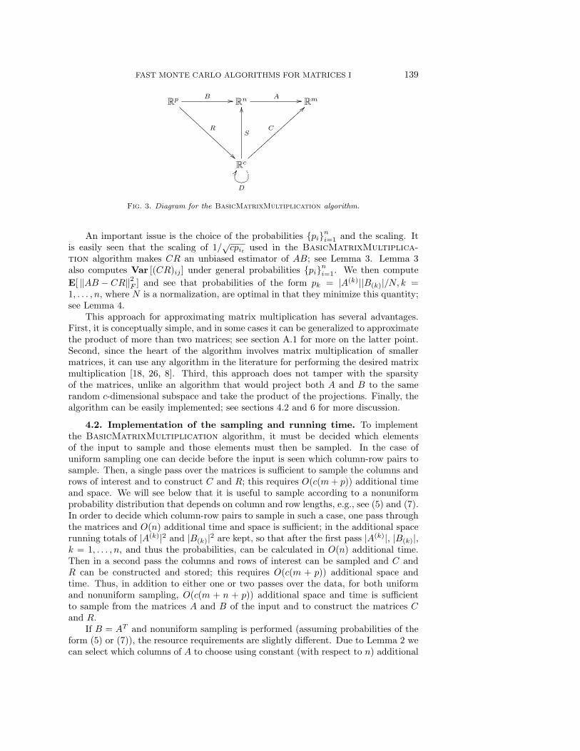
so that CR = ASD(SD)TB ≈ AB. Figure 3 presents a diagram illustrating the actionof the BasicMatrixMultiplication algorithm. The product AB is shown as B andthen A operating between the high-dimensional R
p and Rm via the high-dimensional
Rn; this is approximated by CR, which is shown as R and then C operating between
Rp and R
m via the low-dimensional subspace Rc. Also shown are the sampling matrix
S and the diagonal rescaling matrix D.
FAST MONTE CARLO ALGORITHMS FOR MATRICES I 139
Rp B ��
R
�����
����
����
����
� Rn A ��
Rm
Rc
S
��
C
�������������������
D
��
Fig. 3. Diagram for the BasicMatrixMultiplication algorithm.
An important issue is the choice of the probabilities {pi}ni=1 and the scaling. Itis easily seen that the scaling of 1/
√cpit used in the BasicMatrixMultiplica-
tion algorithm makes CR an unbiased estimator of AB; see Lemma 3. Lemma 3also computes Var [(CR)ij ] under general probabilities {pi}ni=1. We then compute
E[ ‖AB − CR‖2F ] and see that probabilities of the form pk = |A(k)||B(k)|/N, k =
1, . . . , n, where N is a normalization, are optimal in that they minimize this quantity;see Lemma 4.
This approach for approximating matrix multiplication has several advantages.First, it is conceptually simple, and in some cases it can be generalized to approximatethe product of more than two matrices; see section A.1 for more on the latter point.Second, since the heart of the algorithm involves matrix multiplication of smallermatrices, it can use any algorithm in the literature for performing the desired matrixmultiplication [18, 26, 8]. Third, this approach does not tamper with the sparsityof the matrices, unlike an algorithm that would project both A and B to the samerandom c-dimensional subspace and take the product of the projections. Finally, thealgorithm can be easily implemented; see sections 4.2 and 6 for more discussion.
4.2. Implementation of the sampling and running time. To implementthe BasicMatrixMultiplication algorithm, it must be decided which elementsof the input to sample and those elements must then be sampled. In the case ofuniform sampling one can decide before the input is seen which column-row pairs tosample. Then, a single pass over the matrices is sufficient to sample the columns androws of interest and to construct C and R; this requires O(c(m + p)) additional timeand space. We will see below that it is useful to sample according to a nonuniformprobability distribution that depends on column and row lengths, e.g., see (5) and (7).In order to decide which column-row pairs to sample in such a case, one pass throughthe matrices and O(n) additional time and space is sufficient; in the additional spacerunning totals of |A(k)|2 and |B(k)|2 are kept, so that after the first pass |A(k)|, |B(k)|,k = 1, . . . , n, and thus the probabilities, can be calculated in O(n) additional time.Then in a second pass the columns and rows of interest can be sampled and C andR can be constructed and stored; this requires O(c(m + p)) additional space andtime. Thus, in addition to either one or two passes over the data, for both uniformand nonuniform sampling, O(c(m + n + p)) additional space and time is sufficientto sample from the matrices A and B of the input and to construct the matrices Cand R.
If B = AT and nonuniform sampling is performed (assuming probabilities of theform (5) or (7)), the resource requirements are slightly different. Due to Lemma 2 wecan select which columns of A to choose using constant (with respect to n) additional
140 PETROS DRINEAS, RAVI KANNAN, AND MICHAEL W. MAHONEY
space and time during the first pass. Then, during the second pass, these columnsmay be extracted and the matrices C and R = CT may be constructed using O(cm)additional space and time; this will be used in the LinearTimeSVD algorithm of[11]. Note that if only a constant-sized part of the columns of C is needed, as, forexample, in the ConstantTimeSVD algorithm of [11], then extracting and storingthis constant-sized subset of the samples desired may be performed using constantadditional space and time.
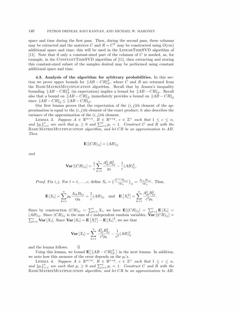
4.3. Analysis of the algorithm for arbitrary probabilities. In this sec-tion we prove upper bounds for ‖AB − CR‖2
F , where C and R are returned fromthe BasicMatrixMultiplication algorithm. Recall that by Jensen’s inequalitybounding ‖AB − CR‖2
F (in expectation) implies a bound for ‖AB − CR‖F . Recallalso that a bound on ‖AB − CR‖F immediately provides a bound on ‖AB − CR‖2
since ‖AB − CR‖2 ≤ ‖AB − CR‖F .Our first lemma proves that the expectation of the (i, j)th element of the ap-
proximation is equal to the (i, j)th element of the exact product; it also describes thevariance of the approximation of the (i, j)th element.
Lemma 3. Suppose A ∈ Rm×n, B ∈ R
n×p, c ∈ Z+ such that 1 ≤ c ≤ n,
and {pi}ni=1 are such that pi ≥ 0 and∑n
i=1 pi = 1. Construct C and R with theBasicMatrixMultiplication algorithm, and let CR be an approximation to AB.Then
E [(CR)ij ] = (AB)ij
and
Var [(CR)ij ] =1
c
n∑k=1
A2ikB
2kj
pk− 1
c(AB)2ij .
Proof. Fix i, j. For t = 1, . . . , c, define Xt =(A(it)B(it)
cpit
)ij
=AiitBitj
cpit. Thus,
E [Xt] =
n∑k=1
pkAikBkj
cpk=
1
c(AB)ij and E
[X2
t
]=
n∑k=1
A2ikB
2kj
c2pk.
Since by construction (CR)ij =∑c
t=1 Xt, we have E [(CR)ij ] =∑c
t=1 E [Xt] =(AB)ij . Since (CR)ij is the sum of c independent random variables, Var [(CR)ij ] =∑c
t=1 Var [Xt]. Since Var [Xt] = E[X2
t
]− E [Xt]
2, we see that
Var [Xt] =
n∑k=1
A2ikB
2kj
c2pk− 1
c2(AB)2ij
and the lemma follows.Using this lemma, we bound E
[‖AB − CR‖2
F
]in the next lemma. In addition,
we note how this measure of the error depends on the pi’s.Lemma 4. Suppose A ∈ R
m×n, B ∈ Rn×p, c ∈ Z
+ such that 1 ≤ c ≤ n,and {pi}ni=1 are such that pi ≥ 0 and
∑ni=1 pi = 1. Construct C and R with the
BasicMatrixMultiplication algorithm, and let CR be an approximation to AB.
FAST MONTE CARLO ALGORITHMS FOR MATRICES I 141
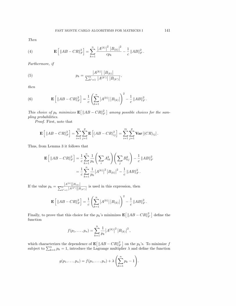
Then
E[‖AB − CR‖2
F
]=
n∑k=1
∣∣A(k)∣∣2 ∣∣B(k)
∣∣2cpk
− 1
c‖AB‖2
F .(4)
Furthermore, if
pk =
∣∣A(k)∣∣ ∣∣B(k)
∣∣∑nk′=1
∣∣A(k′)∣∣ ∣∣B(k′)
∣∣ ,(5)
then
E[‖AB − CR‖2
F
]=
1
c
(n∑
k=1
∣∣A(k)∣∣ ∣∣B(k)
∣∣)2
− 1
c‖AB‖2
F .(6)
This choice of pk minimizes E[‖AB − CR‖2
F
]among possible choices for the sam-
pling probabilities.Proof. First, note that
E[‖AB − CR‖2
F
]=
m∑i=1
p∑j=1
E[(AB − CR)
2ij
]=
m∑i=1
p∑j=1
Var [(CR)ij ] .
Thus, from Lemma 3 it follows that
E[‖AB − CR‖2
F
]=
1
c
n∑k=1
1
pk
(∑i
A2ik
)(∑j
B2kj
)− 1
c‖AB‖2
F
=1
c
n∑k=1
1
pk
∣∣A(k)∣∣2 ∣∣B(k)
∣∣2 − 1
c‖AB‖2
F .
If the value pk =|A(k)||B(k)|∑n
k′=1|A(k′)||B(k′)| is used in this expression, then
E[‖AB − CR‖2
F
]=
1
c
(n∑
k=1
∣∣A(k)∣∣ ∣∣B(k)
∣∣)2
− 1
c‖AB‖2
F .
Finally, to prove that this choice for the pk’s minimizes E[‖AB − CR‖2
F
]define the
function
f(p1, . . . , pn) =
n∑k=1
1
pk
∣∣A(k)∣∣2 ∣∣B(k)
∣∣2 ,which characterizes the dependence of E
[‖AB − CR‖2
F
]on the pk’s. To minimize f
subject to∑n
k=1 pk = 1, introduce the Lagrange multiplier λ and define the function
g(p1, . . . , pn) = f(p1, . . . , pn) + λ
(n∑
k=1
pk − 1
).
142 PETROS DRINEAS, RAVI KANNAN, AND MICHAEL W. MAHONEY
We then have at the minimum that
0 =∂g
∂pi=
−1
p2i
∣∣A(i)∣∣2 ∣∣B(i)
∣∣2 + λ.
Thus,
pi =
∣∣A(i)∣∣ ∣∣B(i)
∣∣√λ
=
∣∣A(i)∣∣ ∣∣B(i)
∣∣∑ni′=1
∣∣A(i′)∣∣ ∣∣B(i′)
∣∣ ,where the second equality comes from solving for
√λ in
∑n−1k=1 pk = 1. That these prob-
abilities are a minimum follows since ∂2g∂pi
2 > 0 ∀i such that |A(i)|2|B(i)|2 >0.
4.4. Analysis of the algorithm for nearly optimal probabilities. WithLemma 4 and using Jensen’s inequality, upper bounds on quantities such as E
[‖AB−
CR‖2F
]and E
[‖AB − CR‖F
]may be obtained for various sampling probabilities
{pi}ni=1. In many cases, by using a martingale argument to show that the erroris tightly concentrated around its mean, the expectations in these bounds may beremoved and the corresponding results can be shown to hold with high probability.
Rather than presenting these results in their full generality, we restrict our at-tention to two particular sets of probabilities. We will say that the sampling prob-
abilities pk =|A(k)||B(k)|∑n
k′=1|A(k′)||B(k′)| are the optimal probabilities since they minimize
E[‖AB − CR‖2
F
], which as Lemma 4 shows is one natural measure of the error. We
will say that a set of sampling probabilities {pi}ni=1 are nearly optimal probabilities if
pk ≥ β|A(k)||B(k)|∑n
k′=1|A(k′)||B(k′)| for some positive constant β ≤ 1.
We now prove, for nearly optimal sampling probabilities, results analogous tothose of Lemma 4, and also that the corresponding results with the expectationsremoved hold with high probability. Notice that if β = 1, then we suffer a smallβ-dependent loss in accuracy.
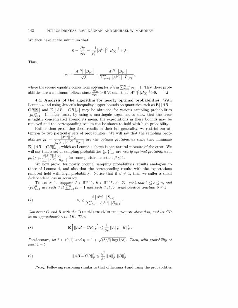
Theorem 1. Suppose A ∈ Rm×n, B ∈ R
n×p, c ∈ Z+ such that 1 ≤ c ≤ n, and
{pi}ni=1 are such that∑n
i=1 pi = 1 and such that for some positive constant β ≤ 1
pk ≥β∣∣A(k)
∣∣ ∣∣B(k)
∣∣∑nk′=1
∣∣A(k′)∣∣ ∣∣B(k′)
∣∣ .(7)
Construct C and R with the BasicMatrixMultiplication algorithm, and let CRbe an approximation to AB. Then
E[‖AB − CR‖2
F
]≤ 1
βc‖A‖2
F ‖B‖2F .(8)
Furthermore, let δ ∈ (0, 1) and η = 1 +√
(8/β) log(1/δ). Then, with probability atleast 1 − δ,
‖AB − CR‖2F ≤ η2
βc‖A‖2
F ‖B‖2F .(9)
Proof. Following reasoning similar to that of Lemma 4 and using the probabilities
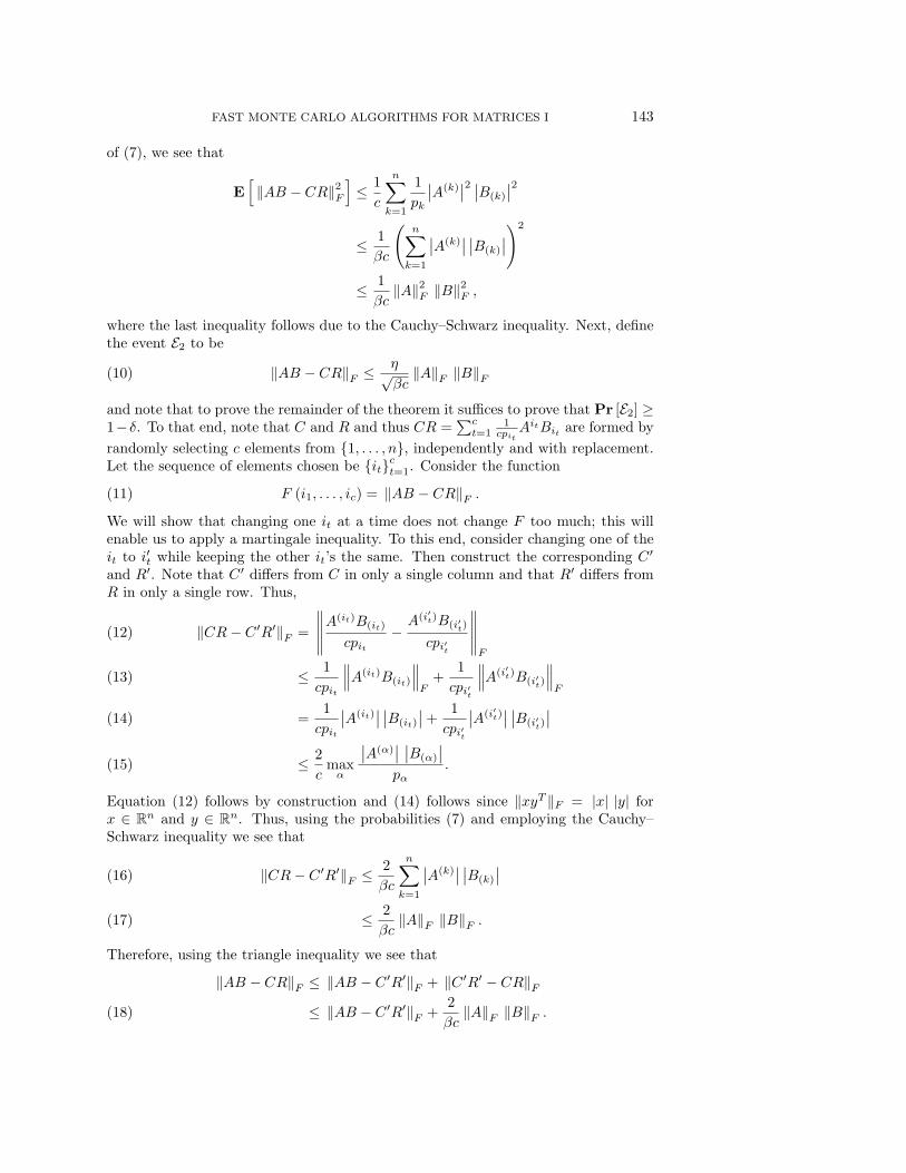
FAST MONTE CARLO ALGORITHMS FOR MATRICES I 143
of (7), we see that
E[‖AB − CR‖2
F
]≤ 1
c
n∑k=1
1
pk
∣∣A(k)∣∣2 ∣∣B(k)
∣∣2
≤ 1
βc
(n∑
k=1
∣∣A(k)∣∣ ∣∣B(k)
∣∣)2
≤ 1
βc‖A‖2
F ‖B‖2F ,
where the last inequality follows due to the Cauchy–Schwarz inequality. Next, definethe event E2 to be
‖AB − CR‖F ≤ η√βc
‖A‖F ‖B‖F(10)
and note that to prove the remainder of the theorem it suffices to prove that Pr [E2] ≥1−δ. To that end, note that C and R and thus CR =
∑ct=1
1cpit
AitBit are formed by
randomly selecting c elements from {1, . . . , n}, independently and with replacement.Let the sequence of elements chosen be {it}ct=1. Consider the function
F (i1, . . . , ic) = ‖AB − CR‖F .(11)
We will show that changing one it at a time does not change F too much; this willenable us to apply a martingale inequality. To this end, consider changing one of theit to i′t while keeping the other it’s the same. Then construct the corresponding C ′
and R′. Note that C ′ differs from C in only a single column and that R′ differs fromR in only a single row. Thus,
‖CR− C ′R′‖F =
∥∥∥∥∥A(it)B(it)
cpit−
A(i′t)B(i′t)
cpi′t
∥∥∥∥∥F
(12)
≤ 1
cpit
∥∥∥A(it)B(it)
∥∥∥F
+1
cpi′t
∥∥∥A(i′t)B(i′t)
∥∥∥F
(13)
=1
cpit
∣∣A(it)∣∣ ∣∣B(it)
∣∣+ 1
cpi′t
∣∣A(i′t)∣∣ ∣∣B(i′t)
∣∣(14)
≤ 2
cmaxα
∣∣A(α)∣∣ ∣∣B(α)
∣∣pα
.(15)
Equation (12) follows by construction and (14) follows since ‖xyT ‖F = |x| |y| forx ∈ R
n and y ∈ Rn. Thus, using the probabilities (7) and employing the Cauchy–
Schwarz inequality we see that
‖CR− C ′R′‖F ≤ 2
βc
n∑k=1
∣∣A(k)∣∣ ∣∣B(k)
∣∣(16)
≤ 2
βc‖A‖F ‖B‖F .(17)
Therefore, using the triangle inequality we see that
‖AB − CR‖F ≤ ‖AB − C ′R′‖F + ‖C ′R′ − CR‖F≤ ‖AB − C ′R′‖F +
2
βc‖A‖F ‖B‖F .(18)
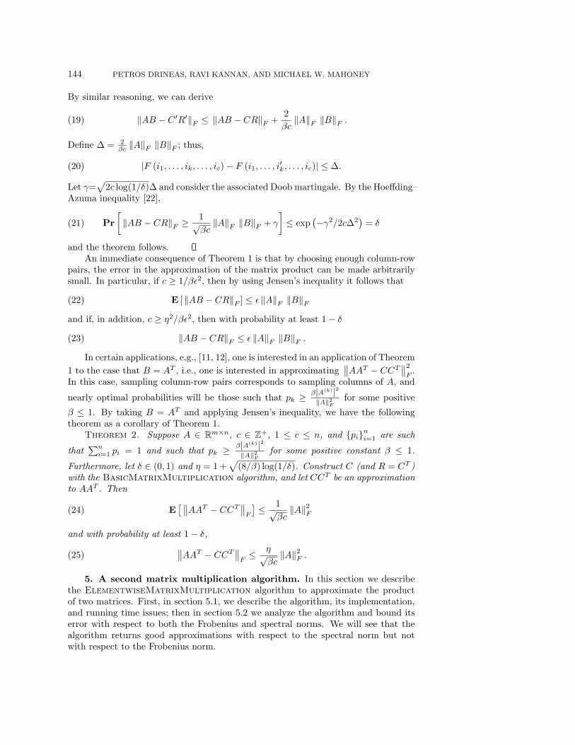
144 PETROS DRINEAS, RAVI KANNAN, AND MICHAEL W. MAHONEY
By similar reasoning, we can derive
‖AB − C ′R′‖F ≤ ‖AB − CR‖F +2
βc‖A‖F ‖B‖F .(19)
Define Δ = 2βc ‖A‖F ‖B‖F ; thus,
|F (i1, . . . , ik, . . . , ic) − F (i1, . . . , i′k, . . . , ic)| ≤ Δ.(20)
Let γ=√
2c log(1/δ)Δ and consider the associated Doob martingale. By the Hoeffding–Azuma inequality [22],
Pr
[‖AB − CR‖F ≥ 1√
βc‖A‖F ‖B‖F + γ
]≤ exp
(−γ2/2cΔ2
)= δ(21)
and the theorem follows.An immediate consequence of Theorem 1 is that by choosing enough column-row
pairs, the error in the approximation of the matrix product can be made arbitrarilysmall. In particular, if c ≥ 1/βε2, then by using Jensen’s inequality it follows that
E [ ‖AB − CR‖F ] ≤ ε ‖A‖F ‖B‖F(22)
and if, in addition, c ≥ η2/βε2, then with probability at least 1 − δ
‖AB − CR‖F ≤ ε ‖A‖F ‖B‖F .(23)
In certain applications, e.g., [11, 12], one is interested in an application of Theorem
1 to the case that B = AT , i.e., one is interested in approximating∥∥AAT − CCT
∥∥2
F.
In this case, sampling column-row pairs corresponds to sampling columns of A, and
nearly optimal probabilities will be those such that pk ≥ β|A(k)|2‖A‖2
F
for some positive
β ≤ 1. By taking B = AT and applying Jensen’s inequality, we have the followingtheorem as a corollary of Theorem 1.
Theorem 2. Suppose A ∈ Rm×n, c ∈ Z
+, 1 ≤ c ≤ n, and {pi}ni=1 are such
that∑n
i=1 pi = 1 and such that pk ≥ β|A(k)|2‖A‖2
F
for some positive constant β ≤ 1.
Furthermore, let δ ∈ (0, 1) and η = 1 +√
(8/β) log(1/δ). Construct C (and R = CT )with the BasicMatrixMultiplication algorithm, and let CCT be an approximationto AAT . Then
E[ ∥∥AAT − CCT
∥∥F
]≤ 1√
βc‖A‖2
F(24)
and with probability at least 1 − δ,∥∥AAT − CCT∥∥F≤ η√
βc‖A‖2
F .(25)
5. A second matrix multiplication algorithm. In this section we describethe ElementwiseMatrixMultiplication algorithm to approximate the productof two matrices. First, in section 5.1, we describe the algorithm, its implementation,and running time issues; then in section 5.2 we analyze the algorithm and bound itserror with respect to both the Frobenius and spectral norms. We will see that thealgorithm returns good approximations with respect to the spectral norm but notwith respect to the Frobenius norm.
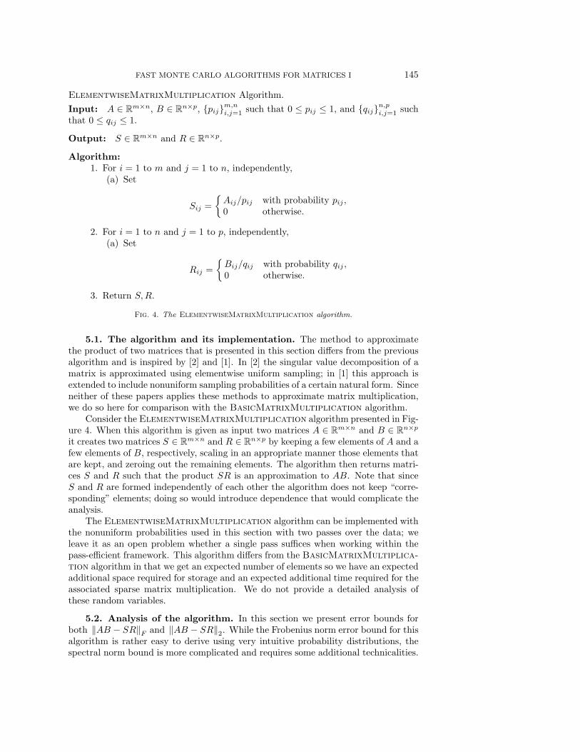
FAST MONTE CARLO ALGORITHMS FOR MATRICES I 145
ElementwiseMatrixMultiplication Algorithm.
Input: A ∈ Rm×n, B ∈ R
n×p, {pij}m,ni,j=1 such that 0 ≤ pij ≤ 1, and {qij}n,pi,j=1 such
that 0 ≤ qij ≤ 1.
Output: S ∈ Rm×n and R ∈ R
n×p.
Algorithm:1. For i = 1 to m and j = 1 to n, independently,
(a) Set
Sij =
{Aij/pij with probability pij ,0 otherwise.
2. For i = 1 to n and j = 1 to p, independently,(a) Set
Rij =
{Bij/qij with probability qij ,0 otherwise.
3. Return S,R.
Fig. 4. The ElementwiseMatrixMultiplication algorithm.
5.1. The algorithm and its implementation. The method to approximatethe product of two matrices that is presented in this section differs from the previousalgorithm and is inspired by [2] and [1]. In [2] the singular value decomposition of amatrix is approximated using elementwise uniform sampling; in [1] this approach isextended to include nonuniform sampling probabilities of a certain natural form. Sinceneither of these papers applies these methods to approximate matrix multiplication,we do so here for comparison with the BasicMatrixMultiplication algorithm.
Consider the ElementwiseMatrixMultiplication algorithm presented in Fig-ure 4. When this algorithm is given as input two matrices A ∈ R
m×n and B ∈ Rn×p
it creates two matrices S ∈ Rm×n and R ∈ R
n×p by keeping a few elements of A and afew elements of B, respectively, scaling in an appropriate manner those elements thatare kept, and zeroing out the remaining elements. The algorithm then returns matri-ces S and R such that the product SR is an approximation to AB. Note that sinceS and R are formed independently of each other the algorithm does not keep “corre-sponding” elements; doing so would introduce dependence that would complicate theanalysis.
The ElementwiseMatrixMultiplication algorithm can be implemented withthe nonuniform probabilities used in this section with two passes over the data; weleave it as an open problem whether a single pass suffices when working within thepass-efficient framework. This algorithm differs from the BasicMatrixMultiplica-
tion algorithm in that we get an expected number of elements so we have an expectedadditional space required for storage and an expected additional time required for theassociated sparse matrix multiplication. We do not provide a detailed analysis ofthese random variables.
5.2. Analysis of the algorithm. In this section we present error bounds forboth ‖AB − SR‖F and ‖AB − SR‖2. While the Frobenius norm error bound for thisalgorithm is rather easy to derive using very intuitive probability distributions, thespectral norm bound is more complicated and requires some additional technicalities.
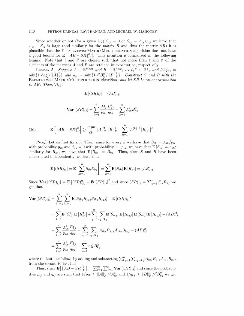
146 PETROS DRINEAS, RAVI KANNAN, AND MICHAEL W. MAHONEY
Since whether or not (for a given i, j) Sij = 0 or Sij = Aij/pij we have thatAij − Sij is large (and similarly for the matrix R and thus the matrix SR) it isplausible that the ElementwiseMatrixMultiplication algorithm does not havea good bound for E
[‖AB − SR‖2
F
]. This intuition is formalized in the following
lemma. Note that � and �′ are chosen such that not more than � and �′ of theelements of the matrices A and B are retained in expectation, respectively.
Lemma 5. Suppose A ∈ Rm×n and B ∈ R
n×p, let �, �′ ∈ Z+, and let pij =
min{1, �A2ij/ ‖A‖2
F } and qij = min{1, �′B2ij/ ‖B‖2
F }. Construct S and R with theElementwiseMatrixMultiplication algorithm, and let SR be an approximationto AB. Then, ∀i, j,
E [(SR)ij ] = (AB)ij ,
Var [(SR)ij ] =
n∑k=1
A2ik
pik
B2kj
qkj−
n∑k=1
A2ikB
2kj
E[‖AB − SR‖2
F
]≥ mpn
��′‖A‖2
F ‖B‖2F −
n∑k=1
∣∣A(k)∣∣2 ∣∣B(k)
∣∣2 .(26)
Proof. Let us first fix i, j. Then, since for every k we have that Sik = Aik/pikwith probability pik and Sik = 0 with probability 1− pik, we have that E [Sik] = Aik;similarly for Rkj , we have that E [Rkj ] = Bkj . Thus, since S and R have beenconstructed independently, we have that
E [(SR)ij ] = E
[n∑
k=1
SikRkj
]=
n∑k=1
E [Sik]E [Rkj ] = (AB)ij .
Since Var [(SR)ij ] = E[(SR)2ij
]− E [(SR)ij ]
2and since (SR)ij =
∑nk=1 SikRkj we
get that
Var [(SR)ij ] =
n∑k1=1
n∑k2=1
E [Sik1Rk1jSik2Rk2j ] − E [(SR)ij ]2
=
n∑k=1
E[S2ik
]E[R2
kj
]+
n∑k1=1
∑k2 �=k1
E [Sik1 ]E [Rk1j ]E [Sik2 ]E [Rk2j ] − (AB)2ij
=
n∑k=1
A2ik
pik
B2kj
qkj+
n∑k1=1
∑k2 �=k1
Aik1Bk1jAik2
Bk2j − (AB)2ij
=
n∑k=1
A2ik
pik
B2kj
qkj−
n∑k=1
A2ikB
2kj ,
where the last line follows by adding and subtracting∑n
k1=1
∑k2=k1
Aik1Bk1jAik2Bk2j
from the second-to-last line.Thus, since E
[‖AB − SR‖2
F
]=∑m
i=1
∑pj=1 Var [(SR)ij ] and since the probabil-
ities pij and qij are such that 1/pik ≥ ‖A‖2F /�A2
ik and 1/qkj ≥ ‖B‖2F /�′B2
kj we get
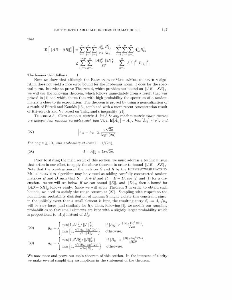
FAST MONTE CARLO ALGORITHMS FOR MATRICES I 147
that
E[‖AB − SR‖2
F
]=
m∑i=1
p∑j=1
n∑k=1
A2ik
pik
B2kj
qkj−
m∑i=1
p∑j=1
n∑k=1
A2ikB
2kj
≥m,p∑i,j=1
n∑k=1
‖A‖2F ‖B‖2
F
��′−
n∑k=1
∣∣A(k)∣∣2 ∣∣B(k)
∣∣2 .The lemma then follows.
Next we show that although the ElementwiseMatrixMultiplication algo-rithm does not yield a nice error bound for the Frobenius norm, it does for the spec-tral norm. In order to prove Theorem 4, which provides our bound on ‖AB − SR‖2,we will use the following theorem, which follows immediately from a result that wasproved in [1] and which shows that with high probability the spectrum of a randommatrix is close to its expectation. The theorem is proved by using a generalization ofa result of Furedi and Komlos [16], combined with a more recent concentration resultof Krivelevich and Vu based on Talagrand’s inequality [21].
Theorem 3. Given an n×n matrix A, let A be any random matrix whose entriesare independent random variables such that ∀i, j, E
[Aij
]= Aij, Var
[Aij
]≤ σ2, and
∣∣∣Aij −Aij
∣∣∣ ≤ σ√
2n
log3 (2n).(27)
For any n ≥ 10, with probability at least 1 − 1/(2n),
‖A− A‖2 < 7σ√
2n.(28)
Prior to stating the main result of this section, we must address a technical issuethat arises in our effort to apply the above theorem in order to bound ‖AB − SR‖2.Note that the construction of the matrices S and R by the ElementwiseMatrix-
Multiplication algorithm may be viewed as adding carefully constructed randommatrices E and D such that S = A + E and R = B + D; see [2] and [1] for a dis-cussion. As we will see below, if we can bound ‖E‖2 and ‖D‖2, then a bound for‖AB − SR‖2 follows easily. Since we will apply Theorem 3 in order to obtain suchbounds, we need to satisfy the range constraint (27). Sampling with respect to thenonuniform probability distribution of Lemma 5 might violate this constraint since,in the unlikely event that a small element is kept, the resulting entry Sij = Aij/pijwill be very large (and similarly for R). Thus, following [1], we modify our samplingprobabilities so that small elements are kept with a slightly larger probability whichis proportional to |Aij | instead of A2
ij :
pij =
⎧⎨⎩
min{1, �A2ij/ ‖A‖2
F } if |Aij | > ‖A‖F log3 (2n)√2n�
,
min{
1,√�|Aij | log3 (2n)√
2n‖A‖F
}otherwise,
(29)
qij =
⎧⎨⎩
min{1, �′B2ij/ ‖B‖2
F } if |Bij | > ‖B‖F log3 (2n)√2n�′
,
min{
1,√�′|Bij | log3 (2n)√
2n‖B‖F
}otherwise.
(30)
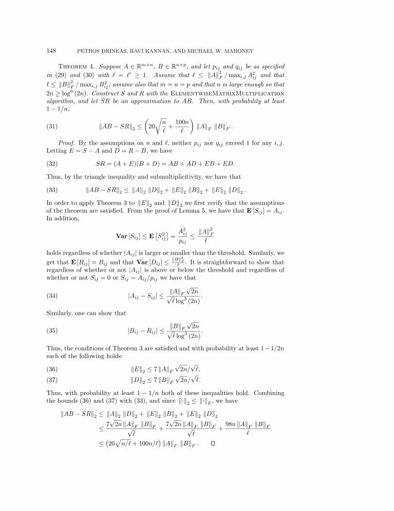
We now state and prove our main theorem of this section. In the interests of claritywe make several simplifying assumptions in the statement of the theorem.
148 PETROS DRINEAS, RAVI KANNAN, AND MICHAEL W. MAHONEY
Theorem 4. Suppose A ∈ Rm×n, B ∈ R
n×p, and let pij and qij be as specified
in (29) and (30) with � = �′ ≥ 1. Assume that � ≤ ‖A‖2F /maxi,j A
2ij and that
� ≤ ‖B‖2F /maxi,j B
2ij; assume also that m = n = p and that n is large enough so that
2n ≥ log6 (2n). Construct S and R with the ElementwiseMatrixMultiplication
algorithm, and let SR be an approximation to AB. Then, with probability at least1 − 1/n,
‖AB − SR‖2 ≤(
20
√n
�+
100n
�
)‖A‖F ‖B‖F .(31)
Proof. By the assumptions on n and �, neither pij nor qij exceed 1 for any i, j.Letting E = S −A and D = R−B, we have
SR = (A + E)(B + D) = AB + AD + EB + ED.(32)
Thus, by the triangle inequality and submultiplicitivity, we have that
‖AB − SR‖2 ≤ ‖A‖2 ‖D‖2 + ‖E‖2 ‖B‖2 + ‖E‖2 ‖D‖2 .(33)
In order to apply Theorem 3 to ‖E‖2 and ‖D‖2 we first verify that the assumptionsof the theorem are satisfied. From the proof of Lemma 5, we have that E [Sij ] = Aij .In addition,
Var [Sij ] ≤ E[S2ij
]=
A2ij
pij≤ ‖A‖2
F
�
holds regardless of whether |Aij | is larger or smaller than the threshold. Similarly, we
get that E [Rij ] = Bij and that Var [Dij ] ≤ ‖B‖2F
� . It is straightforward to show thatregardless of whether or not |Aij | is above or below the threshold and regardless ofwhether or not Sij = 0 or Sij = Aij/pij we have that
|Aij − Sij | ≤‖A‖F
√2n√
� log3 (2n).(34)
Similarly, one can show that
|Bij −Rij | ≤‖B‖F
√2n√
� log3 (2n).(35)
Thus, the conditions of Theorem 3 are satisfied and with probability at least 1−1/2neach of the following holds:
‖E‖2 ≤ 7 ‖A‖F√
2n/√�,(36)
‖D‖2 ≤ 7 ‖B‖F√
2n/√�.(37)
Thus, with probability at least 1 − 1/n both of these inequalities hold. Combiningthe bounds (36) and (37) with (33), and since ‖·‖2 ≤ ‖·‖F , we have
‖AB − SR‖2 ≤ ‖A‖2 ‖D‖2 + ‖E‖2 ‖B‖2 + ‖E‖2 ‖D‖2
≤ 7√
2n ‖A‖F ‖B‖F√�
+7√
2n ‖A‖F ‖B‖F√�
+98n ‖A‖F ‖B‖F
�
≤(20√n/� + 100n/�
)‖A‖F ‖B‖F .
FAST MONTE CARLO ALGORITHMS FOR MATRICES I 149
Notice that if we let � = cn in Theorem 4, then the error bound (31) becomes
‖AB − SR‖2 ≤(
20√c
+100
c
)‖A‖F ‖B‖F = O(1/
√c) ‖A‖F ‖B‖F .
Comparison with (9) of Theorem 1 reveals that (since ‖·‖2 ≤ ‖·‖F ) both of our matrixmultiplication algorithms have, asymptotically, a similar bound with respect to thespectral norm.
6. Discussion and conclusion. To the best of our knowledge, the only previousrandomized algorithm that approximates the product of two matrices is that of Cohenand Lewis [7]. This algorithm is based on random walks in a graph representationof the input matrices and attempts to identify all high-valued entries in nonnegativematrix products in order to improve estimates (relative to exact sparse multiplication)by spending less time on small-valued entries. Their algorithm is more complicatedthan ours, it requires different graph representations of the input matrices if thematrices are allowed to contain negative entries, it needs to store the complete inputmatrices, and it is especially useful when the matrices are not sparse.
It is worth emphasizing how the BasicMatrixMultiplication algorithm be-haves when A and B are well approximated by low-rank matrices. Since a low-rankmatrix or a matrix that is well approximated by a low-rank matrix is a matrix whoserows and columns contain much redundant information in terms of the subspaces theyspan, it is plausible that if the range of B overlaps appropriately with the domain ofA, then we can get a good approximation to AB by carefully sampling a small numberc of appropriately rescaled rank-one approximations to AB. Theorem 1 shows that ifthe {pi}ni=1 are chosen judiciously, then this is the case and Figure 3 illustrates this.
We emphasize that in the case of sampling with nonuniform probabilities oursampling can be viewed as a two-pass algorithm; in the first pass the algorithm readsthe matrix, it then decides which columns and rows to keep, and then in the secondpass it extracts these columns and rows. In certain applications, two passes throughthe matrix are not possible and only one pass is allowed [14]. In these cases, we canstill perform uniform sampling; in this case, if column-row pairs are all approximatelythe same size, i.e., |A(k)||B(k)| is close to its mean value (more precisely, if there existssome positive constant β ≤ 1 such that ∀k |A(k)||B(k)| ≤ 1
βn
∑nk′=1 |A(k′)||B(k′)|),
then the uniform probabilities are nearly optimal and we can sample uniformly witha small β-dependent loss in accuracy.
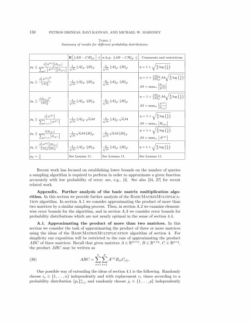
Note that although larger columns and rows get picked more often, the scaling issuch that their weight is deemphasized in the estimator sum. One could imagine asituation when detailed information about the elements of, e.g., A may be obtainedafter a single pass but no information or no information except general bounds on thesize of the elements may be possible for B. In this case, a set of sampling probabil-ities other than those discussed in section 4 may be appropriate. See Table 1 for asummary of the results for different probability distributions; these results are provenin section A.3
The ElementwiseMatrixMultiplication algorithm has been presented forcompleteness and because in some applications its use may be more appropriate thanthe use of the BasicMatrixMultiplication algorithm. It is worth emphasizingthat the ElementwiseMatrixMultiplication algorithm achieves its spectral normbound since its sampling procedure may be viewed as adding a carefully constructedrandom perturbation to every element of the original matrix; see [2, 1] for a nicediscussion of these ideas.
150 PETROS DRINEAS, RAVI KANNAN, AND MICHAEL W. MAHONEY
Table 1
Summary of results for different probability distributions.
E[‖AB − CR‖F
]≤ w.h.p. ‖AB − CR‖F ≤ Comments and restrictions
pk ≥β
∣∣A(k)∣∣|B(k)|∑
k′
∣∣A(k′)∣∣∣∣B(k′)
∣∣ 1√βc
‖A‖F ‖B‖Fη√βc
‖A‖F ‖B‖F η = 1 +
√8β
log(
1δ
)
pk ≥β
∣∣A(k)∣∣2
‖A‖2F
1√βc
‖A‖F ‖B‖Fη√βc
‖A‖F ‖B‖Fη = 1 +
‖A‖F‖B‖F
M√
8β
log(
1δ
)M = maxα
|B(α)||A(α)|
pk ≥ β|B(k)|2‖B‖2
F
1√βc
‖A‖F ‖B‖Fη√βc
‖A‖F ‖B‖Fη = 1 +
‖B‖F‖A‖F
M√
8β
log(
1δ
)M = maxα
|A(α)||B(α)|
pk ≥β
∣∣A(k)∣∣∑n
k′=1
∣∣A(k′)∣∣ 1√
βc‖A‖F
√nM η√
βc‖A‖F
√nM
η = 1 +
√8β
log(
1δ
)M = maxα
∣∣B(α)
∣∣pk ≥ β|B(k)|∑n
k′=1
∣∣B(k′)
∣∣ 1√βc
√nM‖B‖F
η√βc
√nM‖B‖F
η = 1 +
√8β
log(
1δ
)M = maxα
∣∣A(α)∣∣
pk ≥β
∣∣A(k)∣∣|B(k)|
‖A‖F ‖B‖F1√βc
‖A‖F ‖B‖Fη√βc
‖A‖F ‖B‖F η = 1 +
√8β
log(
1δ
)pk = 1
nSee Lemma 11. See Lemma 11. See Lemma 11.
Recent work has focused on establishing lower bounds on the number of queriesa sampling algorithm is required to perform in order to approximate a given functionaccurately with low probability of error; see, e.g., [4]. See also [24, 27] for recentrelated work.
Appendix. Further analysis of the basic matrix multiplication algo-rithm. In this section we provide further analysis of the BasicMatrixMultiplica-
tion algorithm. In section A.1 we consider approximating the product of more thantwo matrices by a similar sampling process. Then, in section A.2 we examine element-wise error bounds for the algorithm, and in section A.3 we consider error bounds forprobability distributions which are not nearly optimal in the sense of section 4.4.
A.1. Approximating the product of more than two matrices. In thissection we consider the task of approximating the product of three or more matricesusing the ideas of the BasicMatrixMultiplication algorithm of section 4. Forsimplicity our exposition will be restricted to the case of approximating the productABC of three matrices. Recall that given matrices A ∈ R
m×n, B ∈ Rn×p, C ∈ R
p×q,the product ABC may be written as
ABC =
n∑s=1
p∑t=1
A(s)BstC(t).(38)
One possible way of extending the ideas of section 4.1 is the following. Randomlychoose is ∈ {1, . . . , n} independently and with replacement c1 times according to aprobability distribution {pi}ni=1 and randomly choose jt ∈ {1, . . . , p} independently
FAST MONTE CARLO ALGORITHMS FOR MATRICES I 151
Rq C ��
C
�����
����
����
����
��R
p B ��R
n A ��R
m
Rc2
S(C,c2)
��
B ��
D{qk}
�� Rc1
S(A,c1)
��
A
�������������������
D{pk}
��
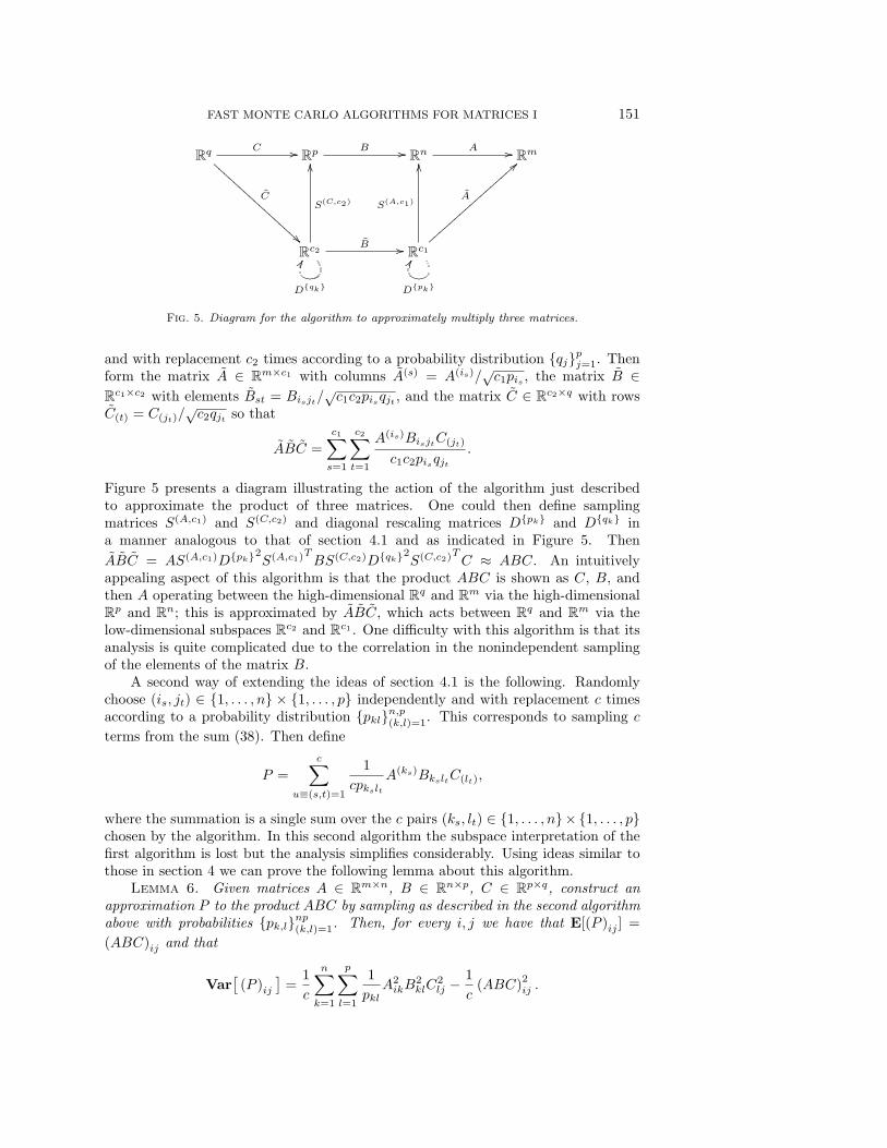
Fig. 5. Diagram for the algorithm to approximately multiply three matrices.
and with replacement c2 times according to a probability distribution {qj}pj=1. Thenform the matrix A ∈ R
m×c1 with columns A(s) = A(is)/√c1pis , the matrix B ∈
Rc1×c2 with elements Bst = Bisjt/
√c1c2pisqjt , and the matrix C ∈ R
c2×q with rowsC(t) = C(jt)/
√c2qjt so that
ABC =
c1∑s=1
c2∑t=1
A(is)BisjtC(jt)
c1c2pisqjt.
Figure 5 presents a diagram illustrating the action of the algorithm just describedto approximate the product of three matrices. One could then define samplingmatrices S(A,c1) and S(C,c2) and diagonal rescaling matrices D{pk} and D{qk} ina manner analogous to that of section 4.1 and as indicated in Figure 5. Then
ABC = AS(A,c1)D{pk}2S(A,c1)
TBS(C,c2)D{qk}2
S(C,c2)TC ≈ ABC. An intuitively
appealing aspect of this algorithm is that the product ABC is shown as C, B, andthen A operating between the high-dimensional R
q and Rm via the high-dimensional
Rp and R
n; this is approximated by ABC, which acts between Rq and R
m via thelow-dimensional subspaces R
c2 and Rc1 . One difficulty with this algorithm is that its
analysis is quite complicated due to the correlation in the nonindependent samplingof the elements of the matrix B.
A second way of extending the ideas of section 4.1 is the following. Randomlychoose (is, jt) ∈ {1, . . . , n} × {1, . . . , p} independently and with replacement c timesaccording to a probability distribution {pkl}n,p(k,l)=1. This corresponds to sampling c
terms from the sum (38). Then define
P =
c∑u≡(s,t)=1
1
cpkslt
A(ks)BksltC(lt),
where the summation is a single sum over the c pairs (ks, lt) ∈ {1, . . . , n}× {1, . . . , p}chosen by the algorithm. In this second algorithm the subspace interpretation of thefirst algorithm is lost but the analysis simplifies considerably. Using ideas similar tothose in section 4 we can prove the following lemma about this algorithm.
Lemma 6. Given matrices A ∈ Rm×n, B ∈ R
n×p, C ∈ Rp×q, construct an
approximation P to the product ABC by sampling as described in the second algorithmabove with probabilities {pk,l}np(k,l)=1. Then, for every i, j we have that E[(P )ij ] =
(ABC)ij and that
Var[(P )ij
]=
1
c
n∑k=1
p∑l=1
1
pklA2
ikB2klC
2lj −
1
c(ABC)
2ij .
152 PETROS DRINEAS, RAVI KANNAN, AND MICHAEL W. MAHONEY
In addition,
E[‖ABC − P‖2
F
]=
1
c
n∑k=1
p∑l=1
1
pkl
∣∣A(k)∣∣2B2
kl
∣∣C(l)
∣∣2 − 1
c‖ABC‖2
F
and the probabilities
pkl =
∣∣A(k)∣∣ |Bkl|
∣∣C(l)
∣∣∑k′∑
l′
∣∣A(k′)∣∣ |Bk′l′ |
∣∣C(l′)
∣∣minimize E
[‖ABC − P‖2
F
]Proof. The proof is similar to those of Lemmas 3 and 4.As in section 4.4 we will define probabilities {pkl} to be nearly optimal if
pkl ≥ β
∣∣A(k)∣∣ |Bkl|
∣∣C(l)
∣∣∑k′∑
l′
∣∣A(k′)∣∣ |Bk′l′ |
∣∣C(l′)
∣∣for some β ≤ 1. If sampling is performed with these probabilities, one can show that
E[‖ABC − P‖2
F
]≤ 1
cβ
∑k
∑l
∣∣A(k)∣∣ |Bkl|
∣∣C(l)
∣∣,and a similar result can be shown to hold with high probability.
Unfortunately, computing the optimal probabilities in the general case is not pass-efficient since it would require O(np) additional space and time. This situation wouldbe relatively worse if one wanted to compute the product of more than three matrices,rendering this method uncompetitive with the exact algorithm. On the other hand,if the matrices are known to have a special structure or if the data are presented ina more specialized format, then this algorithm may be useful. For example, if it isknown that none of the elements of B are too big, i.e., that the elements of B are suchthat there exists a ξB such that ∀i, j we have that Bij ≤ ξB ‖B‖2
F /np, then there willexist a set of probabilities that are nearly optimal that do not depend on B and thatcan be computed efficiently.
A.2. Elementwise error bounds. In this section we provide elementwise errorbounds on |(AB)ij − (CR)ij | for the BasicMatrixMultiplication algorithm fortwo different probability distributions. We have the following lemma.
Lemma 7. Suppose A ∈ Rm×n, B ∈ R
n×p, c ∈ Z+ such that 1 ≤ c ≤ n, and
{pi}ni=1 are such that pi ≥ 0 and∑n
i=1 pi = 1. Let M be such that |Aij | ≤ M and|Bij | ≤ M for every appropriate i, j. Construct C and R with the BasicMatrix-
Multiplication algorithm, and let CR be an approximation to AB. If pk = 1/n forevery k, then for every δ > 0 with probability at least 1 − δ
|(AB)ij − (CR)ij | <nM2
√c
√8 ln(2mp/δ) ∀i, j.(39)
If pk ≥ β|A(k)||B(k)|∑n
k′=1|A(k′)||B(k′)| for some positive constant β ≤ 1, then for every δ > 0 with
probability at least 1 − δ
|(AB)ij − (CR)ij | <n√mpM2
√βc
√(8/β) ln(2mp/δ) ∀i, j.(40)
FAST MONTE CARLO ALGORITHMS FOR MATRICES I 153
Proof. Let us first consider the case of uniform sampling probabilities, i.e., whenpk = 1/n. First, fix attention on one particular (i, j) ∈ ({1, . . . ,m} , {1, . . . , p}). De-
fine X(ij)t =
(A(it)B(it)
cpit
)ij
=AiitBitj
cpit. From Lemma 3 we see that E
[X
(ij)t
]= 1
c (AB)ij .
Define Y(ij)t = X
(ij)t − 1
c (AB)ij , t = 1, . . . , c, and note that the Yt’s are independent
random variables with E[Y
(ij)t
]= 0 for every t = 1, . . . , c. In addition,
∣∣∣Y (ij)t
∣∣∣ ≤∣∣∣∣AiitBitj
cpit
∣∣∣∣+∣∣∣∣1c (AB)ij
∣∣∣∣≤∣∣∣∣AiitBitj
cpit
∣∣∣∣+ nM2
c(41)
≤ 2nM2
c.(42)
Inequality (42) follows since for the uniform probabilities |AiitBitj
cpit| ≤ nM2
c . By com-
bining the upper and lower bounds provided by (42) with Hoeffding’s inequality, wehave that for any t > 0
Pr
[∣∣∣∣∣c∑
t=1
Y(ij)t
∣∣∣∣∣ ≥ ct
]≤ 2 exp
(− 2c2t2∑c
i=1 (4nM2/c)2
)= 2 exp
(− c3t2
8n2M4
).(43)
Define the event Eij to be |∑c
t=1 Y(ij)t | ≥ ct and the event E =
⋃mi=1
⋃pj=1 Eij . If we
then let t = nM2 2√
2c3/2
√ln (2mp/δ), then by (43) we have that Pr [Eij ] ≤ δ
mp . Thus,
(39) then follows since
Pr [E ] ≤m∑i=1
p∑j=1
Pr [Eij ] ≤∑ij
δ/mp = δ.
When applied to the nonuniform probabilities pk ≥ β|A(k)||B(k)|∑n
k′=1|A(k′)||B(k′)| a similar line of
reasoning establishes (40). The key step is to note that when using these probabilitieswe have that∣∣∣∣AiitBitj
cpit
∣∣∣∣ ≤∣∣∣∣∣ AiitBitj
cβ∣∣A(k)
∣∣ ∣∣B(k)
∣∣n∑
k′=1
∣∣A(k′)∣∣ ∣∣B(k′)
∣∣∣∣∣∣∣ ≤
∣∣∣∣n√mp
cβM2
∣∣∣∣ .(44)
Since nM2/c ≤ n√mpM2/(cβ) this, when combined with (41), implies that
∣∣∣Y (ij)t
∣∣∣ ≤ 2n√mpM2
cβ,(45)
which provides the upper and lower bounds on the random variable required to applyHoeffding’s inequality.
When the uniform probabilities are used
‖AB − CR‖2F =
∑ij
|(AB)ij − (CR)ij |2 ≤ mn2pM4
c8 log(2mp/δ)
holds with probability greater than 1− δ. The difference between this result and theresult of Theorem 1 or its variants such as Lemma 11 is that Lemma 7 guarantees that
154 PETROS DRINEAS, RAVI KANNAN, AND MICHAEL W. MAHONEY
every element of the approximation will have small additive error, while Theorem 1provides a tighter Frobenius norm bound but not elementwise guarantees.
It may seem counterintuitive that by sampling with respect to the optimal proba-bilities of section 4 the bound of (40) is worse than that of (39) by a factor of
√mp/β.
(Relatedly, when the nonuniform probabilities of Lemma 7 are used, we have that
‖AB − CR‖2F ≤ m2n2p2M4
β2c8 log(2mp/δ)
with probability greater than 1 − δ.) The reason for this is that the optimal prob-
abilities are optimal with respect to minimizing E[‖AB − CR‖2
F
], in which case
elements corresponding to smaller columns and rows contribute relatively little. Onthe other hand, the two statements of Lemma 7 are required to hold for every i andj. Thus (whether or not the uniform probabilities are nearly optimal) because theoptimal sampling probabilities bias toward elements corresponding to larger columnsand rows an extra factor of
√mp is needed.
A.3. Analysis of the algorithm for nonnearly optimal probabilities.Note that the nearly optimal probabilities (7) use information from both matricesA and B in a particular form. In some cases, such detailed information about bothmatrices may not be available. Thus, we present results for the BasicMatrixMul-
tiplication algorithm for several other sets of probabilities. See Table 1 in section6 for a summary of these results.
In the first case, to estimate the product AB one could use the probabilities(46) which use information from the matrix A only. In this case ‖AB − CR‖F canstill be shown to be small in expectation, and under an additional assumption theexpectation can be removed and the corresponding result can be shown to hold withhigh probability.
Lemma 8. Suppose A ∈ Rm×n, B ∈ R
n×p, c ∈ Z+ such that 1 ≤ c ≤ n, and
{pi}ni=1 are such that∑n
i=1 pi = 1 and such that
pk ≥β∣∣A(k)
∣∣2‖A‖2
F
(46)
for some positive constant β ≤ 1. Construct C and R with the BasicMatrixMul-
tiplication algorithm, and let CR be an approximation to AB. Then
E[‖AB − CR‖2
F
]≤ 1
βc‖A‖2
F ‖B‖2F .(47)
Furthermore, let M= maxα|B(α)||A(α)| , let δ∈(0, 1), and let η = 1+
‖A‖F
‖B‖FM√
(8/β) log(1/δ).
Then with probability at least 1 − δ,
‖AB − CR‖2F ≤ η2
βc‖A‖2
F ‖B‖2F .(48)
Proof. The proof is similar to that of Theorem 1 except that the indicated prob-abilities are used.
Alternatively, to estimate the product AB one could use the probabilities (49)which also use information from the matrix A only, but in a different form than theprobabilities (46). In this case, under an additional assumption ‖AB − CR‖F canstill be shown to be small both in expectation and with high probability.
FAST MONTE CARLO ALGORITHMS FOR MATRICES I 155
Lemma 9. Suppose A ∈ Rm×n, B ∈ R
n×p, c ∈ Z+ such that 1 ≤ c ≤ n, and
{pi}ni=1 are such that∑n
i=1 pi = 1 and such that
pk ≥β∣∣A(k)
∣∣∑nk′=1
∣∣A(k′)∣∣(49)
for some positive constant β ≤ 1. Let M = maxα |B(α)|. Construct C and R with theBasicMatrixMultiplication algorithm, and let CR be an approximation to AB.Then
E[‖AB − CR‖2
F
]≤ 1
βc‖A‖2
F nM2.(50)
Furthermore, let δ ∈ (0, 1) and η = 1 +√
(8/β) log(1/δ). Then with probability atleast 1 − δ,
‖AB − CR‖2F ≤ η2
βc‖A‖2
F nM2.(51)
Proof. The proof is similar to that of Theorem 1 except that the indicated prob-abilities are used.
The probabilities (46) and (49) depend on only the lengths of the columns of A.Results similar to those of the previous two lemmas hold if the probabilities dependon the rows of B rather than the columns of A; see Table 1.
Alternatively, to estimate the product of AB one could use the probabilities (52);interestingly, although the probabilities differ from those of (7) we are able to derivethe same bounds as those of Theorem 1 without additional assumptions.
Lemma 10. Suppose A ∈ Rm×n, B ∈ R
n×p, c ∈ Z+ such that 1 ≤ c ≤ n, and
{pi}ni=1 are such that∑n
i=1 pi = 1 and such that
pk ≥β∣∣A(k)
∣∣ ∣∣B(k)
∣∣‖A‖F ‖B‖F
(52)
for some positive constant β ≤ 1. Construct C and R with the BasicMatrixMul-
tiplication algorithm, and let CR be an approximation to AB. Then
E[‖AB − CR‖2
F
]≤ 1
βc‖A‖2
F ‖B‖2F .(53)
Furthermore, let δ ∈ (0, 1) and η = 1 +√
(8/β) log(1/δ). Then with probability atleast 1 − δ,
‖AB − CR‖2F ≤ η2
βc‖A‖2
F ‖B‖2F .(54)
Proof. The proof is similar to that of Theorem 1 except that the indicated prob-abilities are used.
Of course one could estimate the product AB using the uniform probabilities (55).In this case for simplicity we consider bounding ‖AB − CR‖F directly.
Lemma 11. Suppose A ∈ Rm×n, B ∈ R
n×p, c ∈ Z+ such that 1 ≤ c ≤ n, and
{pi}ni=1 are such that
pk =1
n.(55)
156 PETROS DRINEAS, RAVI KANNAN, AND MICHAEL W. MAHONEY
Construct C and R with the BasicMatrixMultiplication algorithm, and let CRbe an approximation to AB. Then
E [ ‖AB − CR‖F ] ≤√
n
c
(n∑
k=1
∣∣∣A(k)∣∣∣2 ∣∣B(k)
∣∣2)1/2
.(56)
Furthermore, let δ ∈ (0, 1) and γ = n√c
√8 log (1/δ) maxα
∣∣A(α)∣∣ ∣∣B(α)
∣∣. Then with
probability at least 1 − δ,
‖AB − CR‖F ≤√
n
c
(n∑
k=1
∣∣∣A(k)∣∣∣2 ∣∣B(k)
∣∣2)1/2
+ γ.(57)
Proof. The proof is similar to that of Theorem 1 except that the indicated prob-abilities are used.
Acknowledgments. We would like to thank Dimitris Achlioptas for bringingto our attention the results of [21] and the National Science Foundation for partialsupport of this work. In addition, we would like to thank an anonymous reviewer forproviding a careful reading of this paper, for making numerous constructive sugges-tions, and for bringing [28] to our attention.
REFERENCES
[1] D. Achlioptas and F. McSherry, Fast computation of low rank matrix approximations, J.ACM, to appear.
[2] D. Achlioptas and F. McSherry, Fast computation of low rank matrix approximations, inProceedings of the 33rd Annual ACM Symposium on Theory of Computing, 2001, pp. 611–618.
[3] N. Alon, Y. Matias, and M. Szegedy, The space complexity of approximating the frequencymoments, in Proceedings of the 28th Annual ACM Symposium on Theory of Computing,1996, pp. 20–29.
[4] Z. Bar-Yossef, Sampling lower bounds via information theory, in Proceedings of the 35thAnnual ACM Symposium on Theory of Computing, 2003, pp. 335–344.
[5] D. Barbara, C. Faloutsos, J. Hellerstein, Y. Ioannidis, H. V. Jagadish, T. Johnson,
R. Ng, V. Poosala, K. Ross, and K. C. Sevcik, The New Jersey data reduction report,Bulletin of the IEEE Computer Society Technical Committee on Data Engineering, 1997.
[6] R. Bhatia, Matrix Analysis, Springer-Verlag, New York, 1997.[7] E. Cohen and D. D. Lewis, Approximating matrix multiplication for pattern recognition tasks,
J. Algorithms, 30 (1999), pp. 211–252.[8] D. Coppersmith and S. Winograd, Matrix multiplication via arithmetic progressions, J.
Symbolic Comput., 9 (1990), pp. 251–280.[9] P. Drineas and R. Kannan, Fast Monte-Carlo algorithms for approximate matrix multipli-
cation, in Proceedings of the 42nd Annual IEEE Symposium on Foundations of ComputerScience, 2001, pp. 452–459.
[10] P. Drineas and R. Kannan, Pass efficient algorithms for approximating large matrices, inProceedings of the 14th Annual ACM-SIAM Symposium on Discrete Algorithms, 2003,pp. 223–232.
[11] P. Drineas, R. Kannan, and M. W. Mahoney, Fast Monte Carlo algorithms for matricesII: Computing a low-rank approximation to a matrix, SIAM J. Comput., 36 (2006), pp.158–183.
[12] P. Drineas, R. Kannan, and M. W. Mahoney, Fast Monte Carlo algorithms for matricesIII: Computing a compressed approximate matrix decomposition, SIAM J. Comput., 36(2006), pp. 184–206.
[13] P. Drineas, R. Kannan, and M. W. Mahoney, Fast Monte Carlo Algorithms for Matrices I:Approximating Matrix Multiplication, Tech. Report YALEU/DCS/TR-1269, Departmentof Computer Science, Yale University, New Haven, CT, 2004.
FAST MONTE CARLO ALGORITHMS FOR MATRICES I 157
[14] J. Feigenbaum, S. Kannan, M. Strauss, and M. Viswanathan, An approximate L1-difference algorithm for massive data sets, in Proceedings of the 40th Annual IEEE Sym-posium on the Foundations of Computer Science, 1999, pp. 501–511.
[15] A. Frieze, R. Kannan, and S. Vempala, Fast Monte-Carlo algorithms for finding low-rankapproximations, in Proceedings of the 39th Annual IEEE Symposium on Foundations ofComputer Science, 1998, pp. 370–378.
[16] Z. Furedi and J. Komlos, The eigenvalues of random symmetric matrices, Combinatorica, 1(1981), pp. 233–241.
[17] A. C. Gilbert, S. Guha, P. Indyk, Y. Kotidis, S. Muthukrishnan, and M. Strauss, Fast,small-space algorithms for approximate histogram maintenance, in Proceedings of the 34thAnnual ACM Symposium on Theory of Computing, 2002, pp. 389–398.
[18] G. H. Golub and C. F. Van Loan, Matrix Computations, Johns Hopkins University Press,Baltimore, MD, 1989.
[19] M. R. Henzinger, P. Raghavan, and S. Rajagopalan, Computing on Data Streams, Tech.Report 1998-011, Digital Systems Research Center, Palo Alto, CA, 1998.
[20] R. A. Horn and C. R. Johnson, Matrix Analysis, Cambridge University Press, New York,1985.
[21] M. Krivelevich and V. H. Vu, On the Concentration of Eigenvalues of Random SymmetricMatrices, Tech. Report MSR-TR-2000-60, Microsoft Research, Redmond, WA, 2000.
[22] C. McDiarmid, On the method of bounded differences, in Surveys in Combinatorics, 1989,J. Siemons, ed., London Math. Soc. Lecture Notes Ser., Cambridge University Press, Cam-bridge, UK, 1989, pp. 148–188.
[23] J. I. Munro and M. S. Paterson, Selection and sorting with limited storage, in Proceedingsof the 19th Annual IEEE Symposium on Foundations of Computer Science, 1978, pp. 253–258.
[24] M. Rudelson and R. Vershynin, Approximation of Matrices, manuscript.[25] G. W. Stewart and J. G. Sun, Matrix Perturbation Theory, Academic Press, New York,
1990.[26] V. Strassen, Gaussian elimination is not optimal, Numer. Math., 14 (1969), pp. 354–356.[27] R. Vershynin, Coordinate Restrictions of Linear Operators in ln2 , manuscript; available online
from http://arxiv.org/abs/math/0011232.[28] J. S. Vitter, Random sampling with a reservoir, ACM Trans. Math. Softw., 11 (1985), pp. 37–
57.