Fast Solvers for Unsteady Thermal Fluid

Structure Interaction

Philipp Birken×∗, Tobias Gleim†, Detlef Kuhl† and Andreas Meister∗

July 4, 2014

×Centre for the Mathematical Sciences, Numerical Analysis, Lunds University, Box 118,22100 Lund, Sweden

e-mail: philipp.birken@na.lu.se∗Institute of Mathematics, University of Kassel, Heinrich-Plett-Str. 40, 34132 Kassel,

Germany† Institute of Mechanics and Dynamics, University of Kassel, Monchebergstr. 7, 34109

Kassel, Germany

Abstract

We consider time dependent thermal fluid structure interaction. Therespective models are the compressible Navier-Stokes equations and thenonlinear heat equation. A partitioned coupling approach via a Dirichlet-Neumann method and a fixed point iteration is employed. As a refencesolver a previously developed efficient time adaptive higher order timeintegration scheme is used.

To improve upon this, we work on reducing the number of fixed pointcoupling iterations. Thus, first widely used vector extrapolation methodsfor convergence acceleration of the fixed point iteration are tested. Inparticular, Aitken relaxation, minimal polynomial extrapolation (MPE)and reduced rank extrapolation (RRE) are considered. Second, we explorethe idea of extrapolation based on data given from the time integrationand derive such methods for SDIRK2. While the vector extrapolationmethods have no beneficial effects, the extrapolation methods allow toreduce the number of fixed point iterations further by up to a factor oftwo with linear extrapolation performing better than quadratic.

Keywords: Thermal Fluid Structure Interaction, Partitioned Coupling, Con-vergence Acceleration, Extrapolation

1 Introduction

Thermal interaction between fluids and structures plays an important role inmany applications. Examples for this are cooling of gas-turbine blades, thermalanti-icing systems of airplanes [7] or supersonic reentry of vehicles from space[17, 13]. Another is quenching, an industrial heat treatment of metal workpieces.

1

arX

iv:1

407.

0893

v1 [

mat

h.N

A]

3 J

ul 2

014

There, the desired material properties are achieved by rapid local cooling, whichcauses solid phase changes, allowing to create graded materials with preciselydefined properties.

Gas quenching recently received a lot of industrial and scientific interest[25, 12]. In contrast to liquid quenching, this process has the advantage ofminimal environmental impact because of non-toxic quenching media and cleanproducts like air [22]. To exploit the multiple advantages of gas quenching theapplication of computational fluid dynamics has proved essential [2, 22, 16].Thus, we consider the coupling of the compressible Navier-Stokes equations asa model for air, along a non-moving boundary with the nonlinear heat equationas a model for the temperature distribution in steel.

For the solution of the coupled problem, we prefer a partitioned approach [9],where different codes for the sub-problems are reused and the coupling is doneby a master program which calls interface functions of the other codes. Thisallows to use existing software for each sub-problem, in contrast to a monolithicapproach, where a new code is tailored for the coupled equations. To satisfythe boundary conditions at the interface, the subsolvers are iterated in a fixedpoint procedure.

Our goal here is to find a fast solver in this partitioned setting. One approachwould be to speed up the subsolvers and there is active research on that. See[4] for the current situation for fluid solvers. However, we want to approachthe problem from the point of view of a partitioned coupling method, meaningthat we use the subsolvers as they are. As a reference solver, we use the timeadaptive higher order time integration method suggested in [6]. Namely, thesingly diagonally implicit Runge-Kutta (SDIRK) method SDIRK2 is employed.

To improve upon this, one idea is to define the tolerances in the subsolverin a smart way and recently, progress has been made for steady problems [3].However, it is not immediately clear how to transfer these results to the unsteadycase. Thus, the most promising way is to reduce the number of fixed pointiterations, on which we will focus in the present article.

Various methods have been proposed to increase the convergence speed ofthe fixed point iteration by decreasing the interface error between subsequentsteps, for example Relaxation [15, 14], Interface-GMRES [18], ROM-coupling[24] and multigrid coupling [23]. Here, we consider the most standard method,namely Aitken Relaxation and two variants of polynomial vector extrapolation,namely MPE and RRE [21]. These have the merit of being purely algebraic andvery easy to implement.

The second idea we follow is that of extrapolation based on knowledge aboutthe time integration scheme. This has been successfully used in other contexts[1, 8], but has to our knowledge never been tried in Fluid Structure Interaction,where typically little attention is given to the time integration. Here, we uselinear and quadratic extrapolation of old values from the time history, designedspecifically for SDIRK2.

The various methods are compared on the basis of numerical examples,namely the flow past a flat plate, a basic test case for thermal fluid structureinteraction and an example from gas quenching [25].

2

2 Governing Equations

The basic setting we are in is that on a domain Ω1 ⊂ Rd the physics is describedby a fluid model, whereas on a domain Ω2 ⊂ Rd, a different model describingthe structure is used. The two domains are almost disjoint in that they areconnected via an interface. The part of the interface where the fluid and thestructure are supposed to interact is called the coupling interface Γ ⊂ ∂Ω1∪∂Ω2.Note that Γ might be a true subset of the intersection, because the structurecould be insulated. At the interface Γ, coupling conditions are prescribed thatmodel the interaction between fluid and structure. For the thermal couplingproblem, these conditions are that temperature and the normal component ofthe heat flux are continuous across the interface.

2.1 Fluid Model

We model the fluid using the Navier-Stokes equations, which are a second ordersystem of conservation laws (mass, momentum, energy) modeling viscous com-pressible flow. We consider the two dimensional case, written in conservativevariables density ρ, momentum m = ρv and energy per unit volume ρE:

∂tρ+∇ ·m = 0,

∂tmi +

2∑j=1

∂xj(mivj + pδij) =

1

Re

2∑j=1

∂xjSij , i = 1, 2,

∂t(ρE) +∇ · (Hm) =1

Re

2∑j=1

∂xj

(2∑i=1

Sijvi −1

Prqj

).

Here, S = (Sij)i,j=1,2 represents the viscous shear stress tensor and q =(q1, q2)T the heat flux. As the equation are dimensionless, the Reynolds numberRe and the Prandtl number Pr appear. The system is closed by the equationof state for the pressure p = (γ − 1)ρe, the Sutherland law representing thecorrelation between temperature and viscosity as well as the Stokes hypothesis.Additionally, we prescribe appropriate boundary conditions at the boundaryof Ω1 except for Γ, where we have the coupling conditions. In the Dirichlet-Neumann coupling, a temperature value is enforced strongly at Γ.

2.2 Structure Model

Regarding the structure model, we will consider heat conduction only. Thus,we have the nonlinear heat equation for the structure temperature Θ

ρ(x)cp(Θ)d

dtΘ(x, t) = −∇ ·q(x, t), (1)

whereq(x, t) = −λ(Θ)∇Θ(x, t)

3

denotes the heat flux vector. For steel, the specific heat capacity cp and heatconductivity λ are temperature-dependent and highly nonlinear. Here, an em-pirical model for the steel 51CrV4 suggested in [20] is used. This model ischaracterized by the coefficient functions

λ(Θ) = 40.1 + 0.05Θ− 0.0001Θ2 + 4.9 · 10−8Θ3 (2)

and

cp(Θ) = −10 ln

(e−cp1(Θ)/10 + e−cp2(Θ)/10

2

)(3)

with

cp1(Θ) = 34.2e0.0026Θ + 421.15 (4)

and

cp2(Θ) = 956.5e−0.012(Θ−900) + 0.45Θ. (5)

For the mass density one has ρ = 7836 kg/m3. Finally, on the boundary, wehave Neumann conditions q(x, t) ·n(x) = qb(x, t).

3 Discretization

3.1 Discretization in space

Following the partitioned coupling approach, we discretize the two models sep-arately in space. For the fluid, we use a finite volume method, leading to

d

dtu + h(u,Θ) = 0, (6)

where h(u,Θ) represents the spatial discretization and its dependence on thetemperatures in the fluid. In particular, the DLR TAU-Code is employed [10],which is a cell-vertex-type finite volume method with AUSMDV as flux functionand a linear reconstruction to increase the order of accuracy.

Regarding structural mechanics, the use of finite element methods is ubiqui-tious. Therefore, we will also follow that approach here and use quadratic finiteelements [26], leading to the nonlinear equation for all unknowns on Ω2

M(Θ)d

dtΘ + K(Θ)Θ = qb(u). (7)

Here, M is the heat capacity and K the heat conductivity matrix. The vectorΘ consists of all discrete temperature unknowns and qb is the heat flux vectoron the surface. In this case it is the prescribed Neumann heat flux vector of thefluid.

4

3.2 Coupled time integration

For the time integration, a time adaptive SDIRK2 method is implemented ina partitioned way, as suggested in [6]. If the fluid and the solid solver are ableto carry out time steps of implicit Euler type, the master program of the FSIprocedure can be extended to SDIRK methods very easily, since the masterprogram just has to call the backward Euler routines with specific time stepsizes and starting vectors. This method is very efficient and will be used asthe base method in its time adaptive variant, which is much more efficient thanmore commonly used fixed time step size schemes.

To obtain time adaptivity, embedded methods are used. Thereby, the localerror is estimated by the solvers separately, which then report the estimatesback to the master program. Based on this, the new time step is chosen [5]. Tothis end, all stage derivatives are stored by the subsolvers. Furthermore, if thepossibility of rejected time steps is taken into account, the current solution pair(u,Θ) has to be stored as well.

To comply with the conditions that the discrete temperature and heat fluxare continuous at the interface Γ, a Dirichlet-Neumann coupling is used. Thus,the boundary conditions for the two solvers are chosen such that we prescribeNeumann data for one solver and Dirichlet data for the other. Following theanalysis of Giles [11], temperature is prescribed for the equation with smallerheat conductivity, here the fluid, and heat flux is given on Γ for the structure.Choosing these conditions the other way around leads to an unstable scheme.

In the following it is assumed that at time tn, the step size ∆tn is prescribed.Applying a DIRK method to equation (6)-(7) results in the coupled system ofequations to be solved at Runge-Kutta stage i:

F(ui,Θi) := ui − sui −∆tn aiih(ui,Θi) = 0, (8)

T(ui,Θi) := [M−∆tn aiiK]Θi −MsΘi −∆tn aiiqb(ui) = 0. (9)

Here, aii = 1−√

2/2 is a coefficient of the time integration method and sui andsΘi are given vectors, called starting vectors, computed inside the DIRK scheme.

The dependence of the fluid equations h(ui,Θi) on the temperature Θi resultsfrom the nodal temperatures of the structure at the interface. This subset iswritten as ΘΓ

i . Accordingly, the structure equations depend only on the heatflux of the fluid at the coupling interface.

4 Fixed Point Iteration and Improvements

4.1 Basic fixed point iteration

To solve the coupled system of nonlinear equations (8)-(9), a strong coupling ap-proach is employed. Thus, a fixed point iteration is iterated until a convergencecriterion is satisfied. In particular, we use a a nonlinear Gauß-Seidel process:

F(u(ν+1)i ,Θ

(ν)i ) = 0 u

(ν+1)i (10)

T(u(ν+1)i ,Θ

(ν+1)i ) = 0 Θ

(ν+1)i , ν = 0, 1, ... (11)

5

Each inner iteration is thereby done locally by the structure or the fluid solver.More specific, a Newton method is used in the structure and a FAS multigridmethod is employed in the fluid.

In the base method, the starting values of the iteration are given by u(0)i = sui

and Θ(0)i = sΘ

i . The termination criterion is formulated by the relative updateof the nodal temperatures at the interface of the solid structure and we stoponce we are below the tolerance in the time integration scheme divided by five

‖ΘΓ (ν+1)i −Θ

Γ (ν)i ‖ ≤ TOL/5‖ΘΓ (0)

i ‖. (12)

The vector

r(ν+1) := ΘΓ (ν+1)i −Θ

Γ (ν)i (13)

is often referred to as the interface residual.We will now consider different techniques to improve upon this base iter-

ation, namely using vector extrapolation inside the fixed point iteration andthen extrapolation inside the time integration schemes, to obtain better initialvalues.

4.2 Vector Extrapolation

To improve the convergence speed of the fixed point iteration, different vectorextrapolation techniques have been suggested. These are typically classic tech-niques, where a set of k vectors of a convergent vector sequence is extrapolatedto obtain a faster converging sequence. We are now going to describe threetechniques that we will investigate in this framework.

4.2.1 Aitken Relaxation

Relaxation means that after the fixed point iterate is computed, a relaxationstep is added:

ΘΓ (ν+1)

i = ων+1ΘΓ (ν+1)i + (1− ων+1)Θ

Γ (ν)i . (14)

Several strategies exist to compute the relaxation parameter ω.

The idea of Aitken’s method is to enhance the current solution ΘΓ (ν+1)i

using two previous iteration pairs (ΘΓ (ν+2)i ,Θ

Γ (ν+1)i ) and (Θ

Γ (ν+1)i ,Θ

Γ (ν)i )

obtained from the Gauß-Seidel-step (10)-(11). An improvement in the scalarcase is given by the secant method

ΘΓ (ν+1)i =

ΘΓ (ν−1)i Θ

Γ (ν+1)i −Θ

Γ (ν)i Θ

Γ (ν)i

ΘΓ (ν−1)i −Θ

Γ (ν)i −Θ

Γ (ν)i + Θ

Γ (ν+1)i

. (15)

The relaxation factor in equation (14) for the secant method (15) is then

ων+1 =Θ

Γ (ν−1)i −Θ

Γ (ν)i

ΘΓ (ν−1)i −Θ

Γ (ν)i −Θ

Γ (ν)i + Θ

Γ (ν+1)i

. (16)

6

As customary, we use an added recursion on ωi in which we use the old relaxationfactor ων :

ων+1 = −ωνrΓ (ν)

rΓ (ν+1) − rΓ (ν). (17)

In the vector case the division by the residual rΓ (ν+1) − rΓ (ν) is not possible.Therefore, we multiply the nominator and the numerator formally by (rΓ (ν+1)−rΓ (ν))T to obtain

ων+1 = −ων(rΓ (ν))T (rΓ (ν+1) − rΓ (ν))

‖rΓ (ν+1) − rΓ (ν)‖2. (18)

Two previous steps are required to calculate the relaxation parameter. For thefirst fixpoint iteration, the relaxation parameter ω1 must be prescribed. Wechoose ω1 = 0.8, which was reported by other authors to work well.

4.2.2 Polynomial Vector Extrapolation

Another idea we will follow here are Minimal Polynomial Extrapolation (MPE)and Reduced Rank Extrapolation (RRE) [21]. Here, the new approximationis given as a linear combination of existing iterates with coefficients γν to bedetermined:

ΘΓ (ν+1)

i =

ν+1∑j=0

γjΘΓ (j)i . (19)

For MPE, the coefficients are defined via

γj =cj∑ν+1i=0 ci

, j = 0, ..., ν + 1, (20)

where the coefficients cj are the solution of the problem

mincj

∥∥∥ ν+1∑j=0

cjrj + rν+1

∥∥∥2. (21)

For RRE, the coefficients are defined as the solution of the constrained leastsquares problem

minγj

∥∥∥ ν+1∑j=0

γjrj

∥∥∥2

subject to

ν+1∑j=0

γj = 1. (22)

These problems are then solved using a QR decomposition.

4.3 Extrapolation from time integration

To find good starting values for iterative processes in implicit time integra-tion schemes, it is common to use extrapolation based on knowledge about thetrajectory of the solution of the initial value problem [8, 19]. In the spirit of

7

partitioned solvers, we here suggest to use extrapolation of the interface tem-peratures only. Of course, this strategy could be used as well by the subsolvers,but we will not consider this here.

At the first stage, we have the old time step size ∆tn−1 with value Θn−1 andthe current time step size ∆tn with value Θn. We are looking for the value Θ1

at the next stage time tn + c1∆tn. Linear extrapolation results in

Θ1 = Θn + c1∆tn(Θn −Θn−1)/∆tn−1 = (1 +c1∆tn∆tn−1

)Θn −c1∆tn∆tn−1

Θn−1. (23)

Regarding quadratic extrapolation, it is reasonable to choose tn, tn−1 and theintermediate temperature vector Θn−1/2 from the previous stage tn−1+c1∆tn−1.This results in

Θ1 = Θn−1(c1∆tn+(1−c1)∆tn−1)c1∆tn

c1∆t2n−1−Θn−1/2

(c1∆tn+∆tn−1)c1∆tnc1∆t2n−1(1−c1)

+Θn(c1∆tn+∆tn−1)(c1∆tn+(1−c1)∆tn−1)

(1−c1)∆t2n−1. (24)

When applying this idea at the second stage (or at later stages in a schemewith more than two), it is better to use values from the current time interval.Thus, we linearly extrapolate Θn at tn and Θ1 at tn + c1∆t to obtain

Θn+1 = Θn + ∆tn(Θ1 −Θn)/(c1∆tn) = (1− 1

c1)Θn +

1

c1Θ1. (25)

This results in

Θn+1 = Θn−1∆t2n(1−c1)

∆tn−1(∆tn−1+c1∆tn) −Θn(∆tn−1+∆tn)(1−c1)∆tn

∆tn−1c1∆tn

+Θ1(∆tn−1+∆tn)∆tn

(c1∆tn+∆tn−1)c1∆tn. (26)

5 Numerical Results

5.1 Flow over a plate

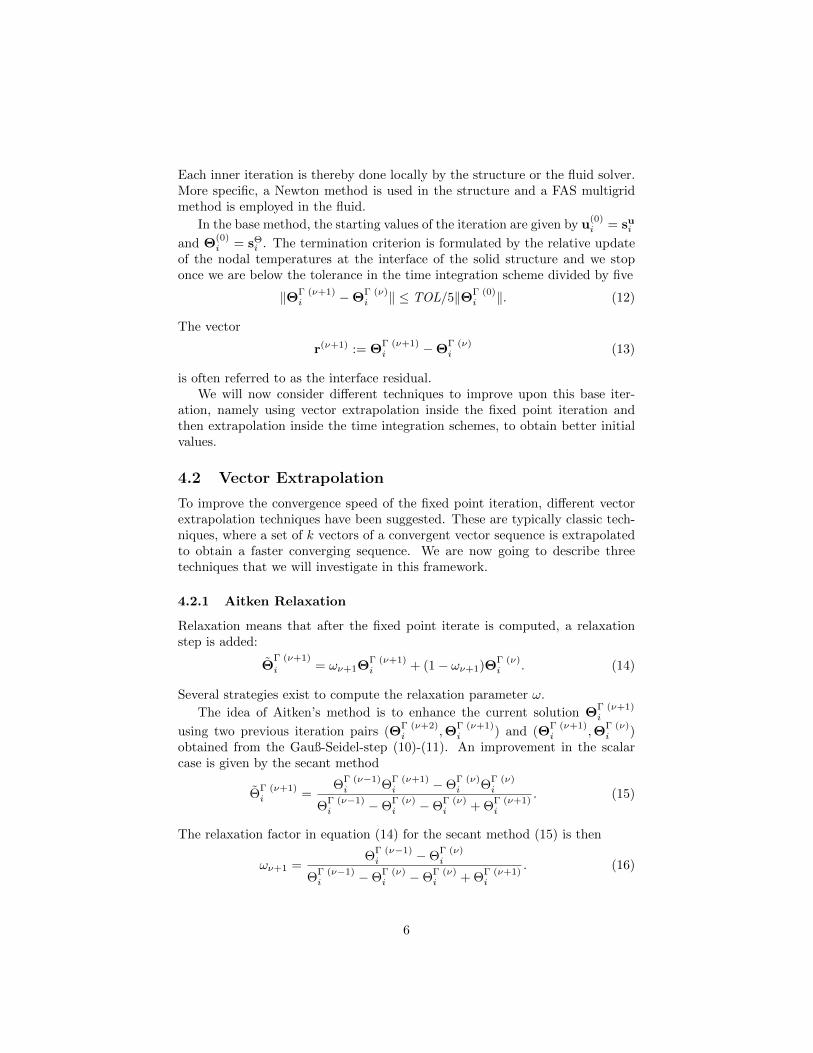
As a first test case, the cooling of a flat plate resembling a simple work piece isconsidered. The work piece is initially at a much higher temperature than thefluid and then cooled by a constant air stream, that is assumed to be laminar,see figure 1.

The inlet is given on the left, where air enters the domain with an initial ve-locity of Ma∞ = 0.8 in horizontal direction and a temperature of 273 K. Then,there are two succeeding regularization regions of 50 mm to obtain an unper-turbed boundary layer. In the first region, 0 ≤ x ≤ 50, symmetry boundaryconditions, vy = 0, q = 0, are applied. In the second region, 50 ≤ x ≤ 100, aconstant wall temperature of 300 K is specified. Within this region the veloc-ity boundary layer fully develops. The third part is the solid (work piece) oflength 200 mm, which exchanges heat with the fluid, but is assumed insulatedotherwise, thus qb = 0. Therefore, Neumann boundary conditions are applied

8

Figure 1: Test case for the coupling method

throughout. Finally, the fluid domain is closed by a second regularization regionof 100 mm with symmetry boundary conditions and the outlet.

Regarding the initial conditions in the structure, a constant temperatureof 900 K at t = 0 s is chosen throughout. To specify reasonable initial condi-tions within the fluid, a steady state solution of the fluid with a constant walltemperature Θ = 900 K is computed.

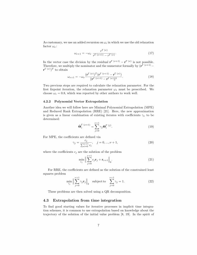
The grid is chosen cartesian and equidistant in the structural part, where in

(a) Entire mesh (b) Mesh zoom

Figure 2: Full grid (left) and zoom into coupling region (right)

the fluid region the thinnest cells are on the boundary and then become coarserin y-direction (see figure 2). To avoid additional difficulties from interpolation,the points of the primary fluid grid, where the heat flux is located in the fluidsolver, and the nodes of the structural grid are chosen to match on the interfaceΓ.

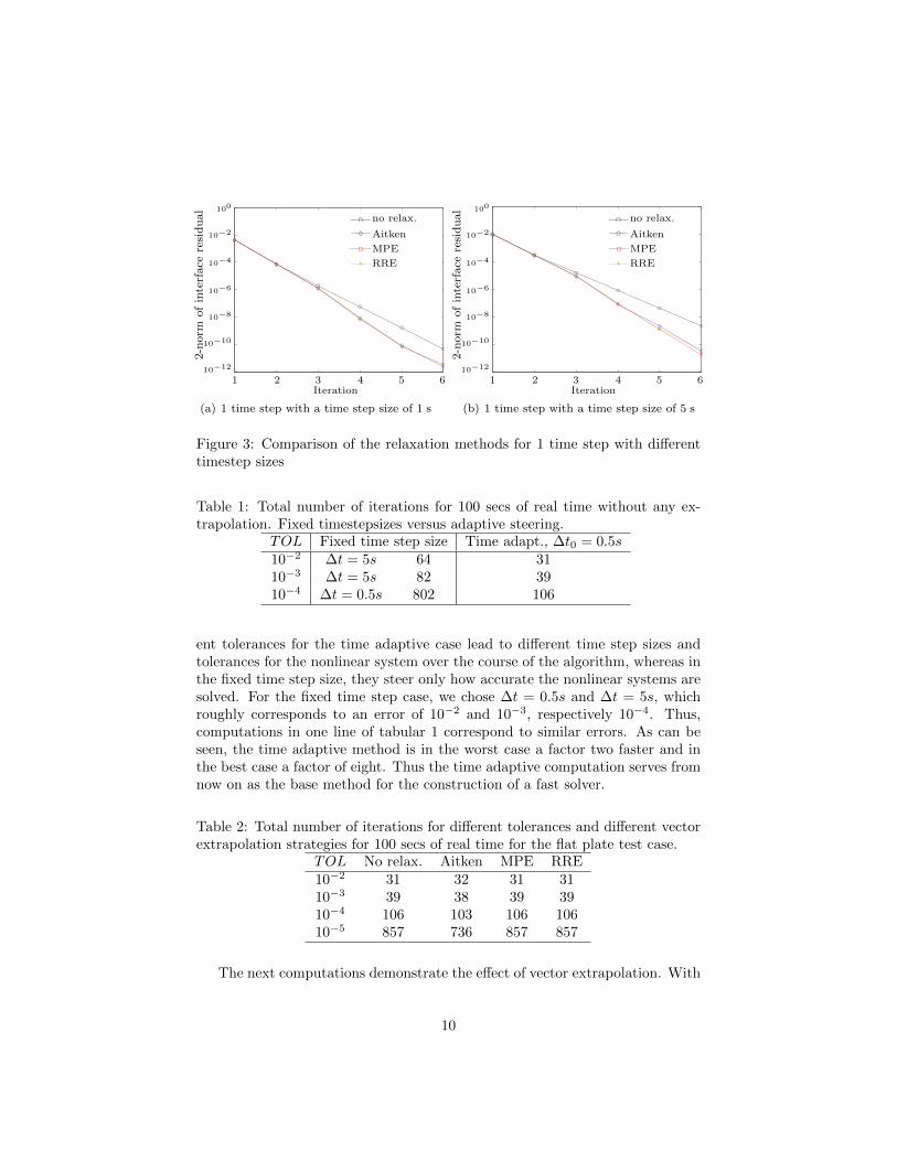
To compare the effect of the different vector extrapolation strategies, weconsider the fixed point equation within the first stage of the first time step inthe test problem with a time step size of ∆t = 1s and ∆t = 5s. In figure 3,we can see how the interface residual decreases with the fixed point iterations.During the first two steps all methods have the same residual norm, since allmethods need at least two iterations to start. For this example, the vectorextrapolation methods outperform the standard scheme for tolerances below10−5.

We now compare the different schemes for a whole simulation of 100 secondsreal time. If not mentioned otherwise, the initial time step size is ∆t = 0.5s.To first give an impression on the effect of the time adaptive method, we lookat fixed time step versus adaptive computations in tabular 1. Thus, the differ-

9

1 2 3 4 5 610-12

10-10

10-8

10-6

10-4

10-2

100

Iteration steps

Res

idua

l erro

r

no relax.AitkenMPERRE

1 2 3 4 5 610-12

10-10

10-8

10-6

10-4

10-2

100

Iteration steps

Res

idua

l erro

r

no relax.AitkenMPERRE

1 2 3 4 5 610-12

10-10

10-8

10-6

10-4

10-2

100

Iteration steps

Res

idua

l erro

r

no relax.AitkenMPERRE

1 2 3 4 5 610-12

10-10

10-8

10-6

10-4

10-2

100

Iteration steps

Res

idua

l erro

r

no relax.AitkenMPERRE

1 2 3 4 5 610-12

10-10

10-8

10-6

10-4

10-2

100

Iteration steps

Res

idua

l erro

r

no relax.AitkenMPERRE

no relax.

Aitken

MPE

RRE

1 2 3 4 5 6Iteration

10−12

10−10

10−8

2-norm

ofinterface

residual

10−6

10−4

10−2

100

(a) 1 time step with a time step size of 1 s

1 2 3 4 5 610-12

10-10

10-8

10-6

10-4

10-2

100

Iteration steps

Res

idua

l erro

r

no relax.AitkenMPERRE

1 2 3 4 5 610-12

10-10

10-8

10-6

10-4

10-2

100

Iteration steps

Res

idua

l erro

r

no relax.AitkenMPERRE

1 2 3 4 5 610-12

10-10

10-8

10-6

10-4

10-2

100

Iteration steps

Res

idua

l erro

r

no relax.AitkenMPERRE

1 2 3 4 5 610-12

10-10

10-8

10-6

10-4

10-2

100

Iteration steps

Res

idua

l erro

r

no relax.AitkenMPERRE

1 2 3 4 5 610-12

10-10

10-8

10-6

10-4

10-2

100

Iteration steps

Res

idua

l erro

r

no relax.AitkenMPERRE

no relax.

Aitken

MPE

RRE

1 2 3 4 5 6Iteration

10−12

10−10

10−8

2-norm

ofinterface

residual

10−6

10−4

10−2

100

(b) 1 time step with a time step size of 5 s

Figure 3: Comparison of the relaxation methods for 1 time step with differenttimestep sizes

Table 1: Total number of iterations for 100 secs of real time without any ex-trapolation. Fixed timestepsizes versus adaptive steering.

TOL Fixed time step size Time adapt., ∆t0 = 0.5s10−2 ∆t = 5s 64 3110−3 ∆t = 5s 82 3910−4 ∆t = 0.5s 802 106

ent tolerances for the time adaptive case lead to different time step sizes andtolerances for the nonlinear system over the course of the algorithm, whereas inthe fixed time step size, they steer only how accurate the nonlinear systems aresolved. For the fixed time step case, we chose ∆t = 0.5s and ∆t = 5s, whichroughly corresponds to an error of 10−2 and 10−3, respectively 10−4. Thus,computations in one line of tabular 1 correspond to similar errors. As can beseen, the time adaptive method is in the worst case a factor two faster and inthe best case a factor of eight. Thus the time adaptive computation serves fromnow on as the base method for the construction of a fast solver.

Table 2: Total number of iterations for different tolerances and different vectorextrapolation strategies for 100 secs of real time for the flat plate test case.

TOL No relax. Aitken MPE RRE10−2 31 32 31 3110−3 39 38 39 3910−4 106 103 106 10610−5 857 736 857 857

The next computations demonstrate the effect of vector extrapolation. With

10

increasing time the time adaptive algorithm chooses larger time step sizes. Thebase method needs more fixed point iterations in the end of the time interval,while the other methods have remained roughly constant. The total numberof fixed point iterations is shown in tabular 2. As we can see, only Aitkenrelaxation has an advantage over the base method and that only for a toleranceof 10−5. For larger tolerances, all the methods need roughly the same numberof iterations, which is also confirmed in Figure 3, where all methods overlap for‖r‖2 ≤ 10−4.

Essentially, the interplay between the fixed point iteration and the timeadaptive scheme results in only two fixed point iterations being necessary pertime step (compare equation (12)). Thus, the vector extrapolation methodshave no effect.

Table 3: Total number of iterations for 100 secs of real time with extrapolationTOL none lin. quad.10−2 31 19 2510−3 39 31 3210−4 106 73 7710−5 857 415 414

Finally, we consider extrapolation based on the time integration scheme. Intable 3, the total number of iterations for 100 seconds of real time is shown.As can be seen, linear extrapolation speeds up the computations between 20%and 50%. Quadratic extrapolation leads to a speedup between 15% and 50%being overall less efficient than the linear extrapolation procedure. Overall,we are thus able to simulate 100 seconds of real time for this problem for anengineering tolerance using only 19 calls to fluid and the structure solver each.

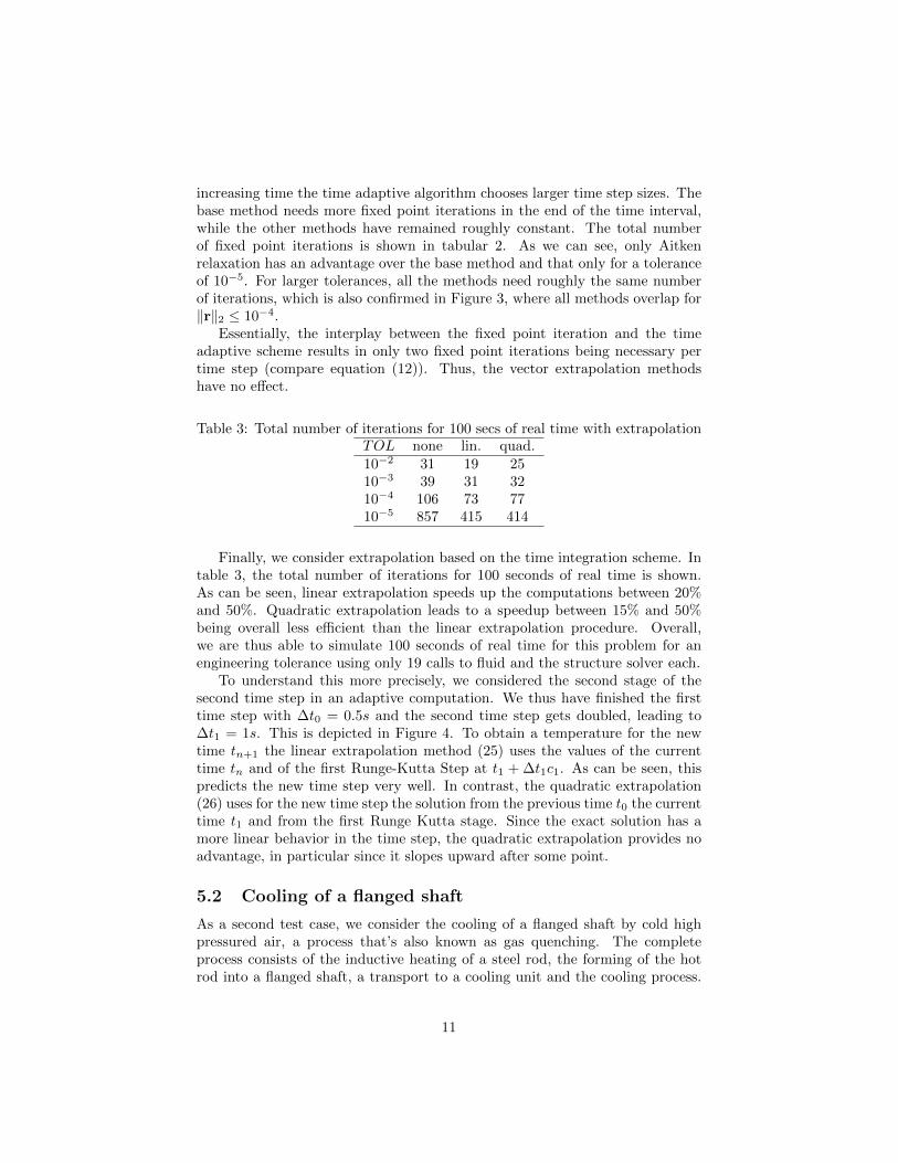
To understand this more precisely, we considered the second stage of thesecond time step in an adaptive computation. We thus have finished the firsttime step with ∆t0 = 0.5s and the second time step gets doubled, leading to∆t1 = 1s. This is depicted in Figure 4. To obtain a temperature for the newtime tn+1 the linear extrapolation method (25) uses the values of the currenttime tn and of the first Runge-Kutta Step at t1 + ∆t1c1. As can be seen, thispredicts the new time step very well. In contrast, the quadratic extrapolation(26) uses for the new time step the solution from the previous time t0 the currenttime t1 and from the first Runge Kutta stage. Since the exact solution has amore linear behavior in the time step, the quadratic extrapolation provides noadvantage, in particular since it slopes upward after some point.

5.2 Cooling of a flanged shaft

As a second test case, we consider the cooling of a flanged shaft by cold highpressured air, a process that’s also known as gas quenching. The completeprocess consists of the inductive heating of a steel rod, the forming of the hotrod into a flanged shaft, a transport to a cooling unit and the cooling process.

11

0 0.5 1 1.5865

870

875

880

885

890

895

900

0 0.5 1 1.5865

870

875

880

885

890

895

900

data1

data2

data3data4

data5

1 2 3 4 5 610-12

10-10

10-8

10-6

10-4

10-2

100

Iteration steps

Res

idua

l erro

r

no relax.AitkenMPERRE

0 0.5 1 1.5865

870

875

880

885

890

895

900

data1

data2

data3

data4

linear extrap.

quad. extrap.

final solns.

0 0.5 1 1.5t [s]

865

870

875

880

Θ [K]

890

895

900

Figure 4: Comparison of the linear and quadratic extrapolation methods for thetime step t = 1.5s.

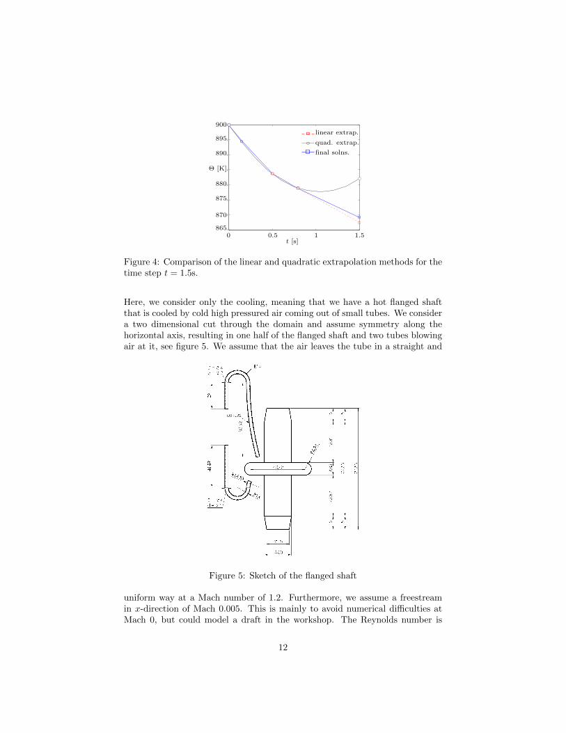
Here, we consider only the cooling, meaning that we have a hot flanged shaftthat is cooled by cold high pressured air coming out of small tubes. We considera two dimensional cut through the domain and assume symmetry along thehorizontal axis, resulting in one half of the flanged shaft and two tubes blowingair at it, see figure 5. We assume that the air leaves the tube in a straight and

Figure 5: Sketch of the flanged shaft

uniform way at a Mach number of 1.2. Furthermore, we assume a freestreamin x-direction of Mach 0.005. This is mainly to avoid numerical difficulties atMach 0, but could model a draft in the workshop. The Reynolds number is

12

Re = 2500 and the Prandtl number Pr = 0.72.

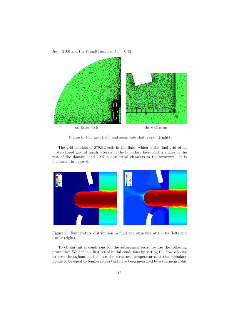
(a) Entire mesh (b) Mesh zoom

Figure 6: Full grid (left) and zoom into shaft region (right)

The grid consists of 279212 cells in the fluid, which is the dual grid of anunstructured grid of quadrilaterals in the boundary layer and triangles in therest of the domain, and 1997 quadrilateral elements in the structure. It isillustrated in figure 6.

Figure 7: Temperature distribution in fluid and structure at t = 0s (left) andt = 1s (right).

To obtain initial conditions for the subsequent tests, we use the followingprocedure: We define a first set of initial conditions by setting the flow velocityto zero throughout and choose the structure temperatures at the boundarypoints to be equal to temperatures that have been measured by a thermographic

13

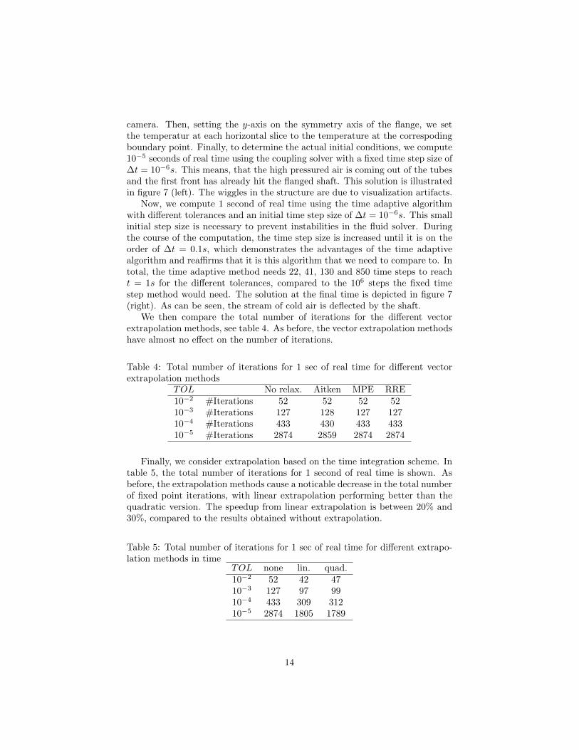
camera. Then, setting the y-axis on the symmetry axis of the flange, we setthe temperatur at each horizontal slice to the temperature at the correspodingboundary point. Finally, to determine the actual initial conditions, we compute10−5 seconds of real time using the coupling solver with a fixed time step size of∆t = 10−6s. This means, that the high pressured air is coming out of the tubesand the first front has already hit the flanged shaft. This solution is illustratedin figure 7 (left). The wiggles in the structure are due to visualization artifacts.

Now, we compute 1 second of real time using the time adaptive algorithmwith different tolerances and an initial time step size of ∆t = 10−6s. This smallinitial step size is necessary to prevent instabilities in the fluid solver. Duringthe course of the computation, the time step size is increased until it is on theorder of ∆t = 0.1s, which demonstrates the advantages of the time adaptivealgorithm and reaffirms that it is this algorithm that we need to compare to. Intotal, the time adaptive method needs 22, 41, 130 and 850 time steps to reacht = 1s for the different tolerances, compared to the 106 steps the fixed timestep method would need. The solution at the final time is depicted in figure 7(right). As can be seen, the stream of cold air is deflected by the shaft.

We then compare the total number of iterations for the different vectorextrapolation methods, see table 4. As before, the vector extrapolation methodshave almost no effect on the number of iterations.

Table 4: Total number of iterations for 1 sec of real time for different vectorextrapolation methods

TOL No relax. Aitken MPE RRE10−2 #Iterations 52 52 52 5210−3 #Iterations 127 128 127 12710−4 #Iterations 433 430 433 43310−5 #Iterations 2874 2859 2874 2874

Finally, we consider extrapolation based on the time integration scheme. Intable 5, the total number of iterations for 1 second of real time is shown. Asbefore, the extrapolation methods cause a noticable decrease in the total numberof fixed point iterations, with linear extrapolation performing better than thequadratic version. The speedup from linear extrapolation is between 20% and30%, compared to the results obtained without extrapolation.

Table 5: Total number of iterations for 1 sec of real time for different extrapo-lation methods in time

TOL none lin. quad.10−2 52 42 4710−3 127 97 9910−4 433 309 31210−5 2874 1805 1789

14

6 Summary and Conclusions

We considered a time dependent thermal fluid structure interaction problemwhere a nonlinear heat equation to model steel is coupled with the compressibleNavier-Stokes equations. The coupling is performed in a Dirichlet-Neumannmanner. As a fast base solver, a higher order time adaptive method is used fortime integration. This method is significantly more efficient than a fixed timestep method and is therefore the scheme to beat.

To reduce the number of fixed point iterations in a partitioned spirit, firstdifferent vector extrapolation techniques, namely Aitken Relaxation, MPE andRRE were compared. These have a negligible effect, since they are only usefulwhen a large number of iterations is needed per system and the time adaptivemethod results in only two iterations being necessary per time step. However,extrapolation based on the time integration method works from the first it-eration and reduces the number of iterations by up to 50%. Hereby, linearextrapolation works better than quadratic.

The combined time adaptive method with linear extrapolation thus allowsto solve real life problems at engineering tolerances using only a couple dozencalls to the fluid and structure solver.

Acknowledgement

Financial support has been provided by the German Research Foundation (DFG)via the Sonderforschungsbereich Transregio 30, projects C1 and C2.

References

[1] M. Arnold, Stability of Sequential Modular Time Integration Methods forCoupled Multibody System Models, J. Comput. Nonlinear Dynam., 5 (2010),pp. 1–9.

[2] A. L. Banka, Practical Applications of CFD in heat processing, HeatTreating Progress, (2005).

[3] P. Birken, Termination criteria for inexact fixed point schemes, Numer.Linear Algebra Appl., submitted.

[4] P. Birken, Numerical Methods for the Unsteady Compressible Navier-Stokes Equations, Habilitation Thesis, University of Kassel, 2012.

[5] P. Birken, K. J. Quint, S. Hartmann, and A. Meister, Chosingnorms in adaptive FSI calculations, PAMM, 10 (2010), pp. 555–556.

[6] , A Time-Adaptive Fluid-Structure Interaction Method for ThermalCoupling, Comp. Vis. in Science, 13 (2011), pp. 331–340.

15

[7] J. M. Buchlin, Convective Heat Transfer and Infrared Thermography, J.Appl. Fluid Mech., 3 (2010), pp. 55–62.

[8] P. Erbts and A. Duster, Accelerated staggered coupling schemes forproblems of thermoelasticity at finite strains, Comp. & Math. with Appl.,64 (2012), pp. 2408–2430.

[9] C. Farhat, CFD-based Nonlinear Computational Aeroelasticity, in Ency-clopedia of Computational Mechanics, E. Stein, R. de Borst, and T. J. R.Hughes, eds., vol. 3: Fluids, John Wiley & Sons, 2004, ch. 13, pp. 459–480.

[10] T. Gerhold, O. Friedrich, J. Evans, and M. Galle, Calculationof Complex Three-Dimensional Configurations Employing the DLR-TAU-Code, AIAA Paper, 97-0167 (1997).

[11] M. B. Giles, Stability Analysis of Numerical Interface Conditions inFluid-Structure Thermal Analysis, Int. J. Num. Meth. in Fluids, 25 (1997),pp. 421–436.

[12] U. Heck, U. Fritsching, and K. Bauckhage, Fluid flow and heattransfer in gas jet quenching of a cylinder, International Journal of Nu-merical Methods for Heat & Fluid Flow, 11 (2001), pp. 36–49.

[13] M. Hinderks and R. Radespiel, Investigation of Hypersonic Gap Flowof a Reentry Nosecap with Consideration of Fluid Structure Interaction,AIAA Paper, 06-1111 (2006).

[14] U. Kuttler and W. A. Wall, Fixed-point fluidstructure interactionsolvers with dynamic relaxation, Comput. Mech., 43 (2008), pp. 61–72.

[15] P. Le Tallec and J. Mouro, Fluid structure interaction with largestructural displacements, Comp. Meth. Appl. Mech. Engrg., 190 (2001),pp. 3039–3067.

[16] N. Lior, The cooling process in gas quenching, J. Materials ProcessingTechnology, 155-156 (2004), pp. 1881–1888.

[17] R. C. Mehta, Numerical Computation of Heat Transfer on Reentry Cap-sules at Mach 5, AIAA-Paper 2005-178, (2005).

[18] C. Michler, E. H. van Brummelen, and R. de Borst, Error-amplification Analysis of Subiteration-Preconditioned GMRES for Fluid-Structure Interaction, Comp. Meth. Appl. Mech. Eng., 195 (2006),pp. 2124–2148.

[19] H. Olsson and G. Soderlind, Stage value predictors and efficient New-ton iterations in implicit Runge-Kutta methods, SIAM J. Sci. Comput., 20(1998), pp. 185–202.

16

[20] K. J. Quint, S. Hartmann, S. Rothe, N. Saba, and K. Steinhoff,Experimental validation of high-order time integration for non-linear heattransfer problems, Comput. Mech., 48 (2011), pp. 81–96.

[21] A. Sidi, Review of two vector extrapolation methods of polynomial type withapplications to large-scale problems, J. Comp. Phys., 3 (2012), pp. 92–101.

[22] P. Stratton, I. Shedletsky, and M. Lee, Gas Quenching with Helium,Solid State Phenomena, 118 (2006), pp. 221–226.

[23] S. van Zuijlen, A. H. Bosscher and H. Bijl, Two level algorithms forpartitioned fluidstructure interaction computations, Comp. methods appl.mech. eng., (2007).

[24] J. Vierendeels, L. Lanoye, J. Degroote, and P. Verdonck, Im-plicit Coupling of Partitioned Fluid-Structure Interaction Problems withReduced Order Models, Comp. & Struct., 85 (2007), pp. 970–976.

[25] U. Weidig, N. Saba, and K. Steinhoff, Massivumformproduktemit funktional gradierten Eigenschaften durch eine differenzielle thermo-mechanische Prozessfuhrung, WT-Online, (2007), pp. 745–752.

[26] O. Zienkiewicz and R. Taylor, The Finite Element Method, Butter-worth Heinemann, 2000.

17