Embed Size (px)
Citation preview

FastExcel SpeedTools User Guide FastExcel SpeedTools 1
FastExcelSpeedTools
FastExcel SpeedTools User Guide Table of Contents 2
TableofContents
FastExcel SpeedTools 1
Table of Contents 2
Overview 7
High-Performance, High-Power Functions 8
Extend your capabilities with over 90 High‐Power Functions ...................................... 8
High‐Performance AVLOOKUP2 family of functions ..................................................... 9
Regular Expression Functions ..................................................................................... 11
High‐Performance FILTER.IFS family of functions....................................................... 11
The Family of LISTDISTINCT Functions ........................................................................ 12
New Family of AND and OR functions designed for Array Formulae. ........................ 13
5 New functions to simplify and extend array‐handling............................................. 13
8 New Text‐handling Functions .................................................................................. 13
6 Dynamic sorting functions ....................................................................................... 13
New Math and Statistics functions ............................................................................. 13
New Calculation Methods & Properties 14
Extended Calculation Modes ...................................................................................... 14
What’s New in FastExcel SpeedTools for FastExcel V2 Users 15
Installing and Activating FastExcel SpeedTools 16
Getting Started with FastExcel SpeedTools 20
SpeedTools Functions 21
Excel Function Wizard ................................................................................................. 21
SpeedTools Functions by Product and Category ........................................................ 24
SpeedTools Functions Properties ............................................................................... 26
SpeedTools Filters: Filtering Functions 28
The FILTER.IFS Multiple Criteria Function Family ....................................................... 29

FastExcel SpeedTools User Guide Table of Contents 3
FILTER.IFS function ...................................................................................................... 31
FILTER.IFS Examples .................................................................................................... 38
FILTER.SORTED function ............................................................................................. 40
FILTER.MATCH function .............................................................................................. 41
ASUMIFS function ....................................................................................................... 42
ACOUNTIFS function ................................................................................................... 43
FILTER.VISIBLE function .............................................................................................. 44
Rgx.COUNTIF function ................................................................................................ 45
Rgx.SUMIF function .................................................................................................... 46
The LISTDISTINCTS family of functions. ...................................................................... 47
LISTDISTINCTS Function .............................................................................................. 48
LISTDISTINCTS.COUNT Function ................................................................................. 50
LISTDISTINCTS.SUM Function ..................................................................................... 51
LISTDISTINCTS.AVG Function ...................................................................................... 52
COUNTDISTINCTS Function ......................................................................................... 53
COUNTDUPES Function ............................................................................................... 54
LISTDISTINCTS Examples ............................................................................................. 55
SpeedTools Filters - Sorting Functions 58
VSORTC – Dynamic text collating Sort of a vertical range or array ............................ 60
Case.VSORTC – Case‐sensitive dynamic Sort of a vertical range or array .................. 61
VSORTB – Fast Dynamic Sort of a vertical range or array ........................................... 62
VSORTC.INDEX – Collating Text Index Sort of a vertical range or array ..................... 63
Case.VSORTC.INDEX – Collating Text Index Sort of a vertical range or array ............. 64
VSORTB.INDEX – Fast Index Sort of a vertical range or array ..................................... 65
SpeedTools Lookups: Lookup Functions 66
Outstanding Performance .......................................................................................... 66
Advanced Function ..................................................................................................... 66
Better, Safer Lookup Defaults ..................................................................................... 67

FastExcel SpeedTools User Guide Table of Contents 4
SpeedTools Lookup Families ....................................................................................... 67
High‐performance exact match Memory Lookups ..................................................... 68
Reconciling lists super‐fast using COMPARE.LISTS ..................................................... 70
The 24 Advanced Function Lookups ........................................................................... 70
MEMLOOKUP Function ............................................................................................... 72
MEMMATCH Function ................................................................................................ 75
COMPARE.LISTS Function ........................................................................................... 78
COMPARE.LISTS Examples .......................................................................................... 80
AVLOOKUP2, AVLOOKUPS2 & AVLOOKUPNTH Functions .......................................... 83
AVLOOKUP2 Examples ................................................................................................ 86
Case.AVLOOKUP2, Case.AVLOOKUPS2 & Case.AVLOOKUPNTH Functions ................ 91
AMATCH2, AMATCHES2 & AMATCHNTH functions ................................................... 95
Case.AMATCH2, Case.AMATCHES2 & Case.AMATCHNTH functions .......................... 99
Rgx.AVLOOKUP2, Rgx.AVLOOKUPS2 & Rgx.AVLOOKUPNTH Functions ................... 103
Rgx.Case.AVLOOKUP2, Rgx.Case.AVLOOKUPS2 & Rgx.Case.AVLOOKUPNTH
Functions ................................................................................................................... 106
Rgx.AMATCH2, Rgx.AMATCHES2 & Rgx.AMATCHNTH functions ............................. 109
Rgx.Case.AMATCH2, Rgx.Case.AMATCHES2 & Rgx.Case.AMATCHNTH functions ... 112
SpeedTools Extras: Mathematical Functions 115
VLINTERP2 function .................................................................................................. 116
LINTERP2D function .................................................................................................. 118
Calculating Gini Coefficients with GINICOEFF ........................................................... 119
GINICOEFF function .................................................................................................. 120
SpeedTools Extras: Logical Functions 121
SpeedTools Logical Functions for Array Formulae ................................................... 122
OR.ROWS, OR.COLS, OR.CELLS, AND.ROWS, AND.COLS, AND.CELLS, ALL, ANY,
NONE ......................................................................................................................... 122
Examples of SpeedTools Logical Functions: .............................................................. 123

FastExcel SpeedTools User Guide Table of Contents 5
IFERRORX Function ................................................................................................... 127
SpeedTools Extras: Reference Functions 129
EVAL function: evaluate a string ............................................................................... 130
PREVIOUS Function ................................................................................................... 131
SETMEM and GETMEM Functions ............................................................................ 133
SpeedTools Extras: Array-Handling Functions 134
COL.ARRAY Function ................................................................................................. 135
ROW.ARRAY Function ............................................................................................... 137
REVERSE.ARRAY Function ......................................................................................... 139
PAD.ARRAY Function ................................................................................................. 141
VECTOR Function ...................................................................................................... 142
SpeedTools Extras: Information Functions 143
ISLIKE array function for pattern‐matching strings .................................................. 144
Rgx.ISLIKE function .................................................................................................... 145
HASFORMULA function ............................................................................................. 146
Calculation Sequence and Counting functions ......................................................... 147
CALCSEQCOUNTREF Function ................................................................................... 147
CALCSEQCOUNTSET Function ................................................................................... 147
CALCSEQCOUNTVOL function ................................................................................... 147
Functions for counting Rows and Columns .............................................................. 149
COUNTROWS Function ............................................................................................. 150
COUNTCONTIGROWS Function ................................................................................ 151
COUNTUSEDROWS Function .................................................................................... 153
COUNTCOLS Function ............................................................................................... 154
COUNTCONTIGCOLS Function .................................................................................. 155
COUNTUSEDCOLS Function ...................................................................................... 157
Examples and comparison of the counting functions .............................................. 157
Using the Count functions in dynamic range names ................................................ 158

FastExcel SpeedTools User Guide Table of Contents 6
SpeedTools Extras: Text Functions 160
CONCAT.RANGE – concatenate range data .............................................................. 161
PAD.TEXT function .................................................................................................... 162
REVERSE.TEXT Function ............................................................................................ 163
SPLIT.TEXT Function .................................................................................................. 164
Rgx.FIND function ..................................................................................................... 165
Rgx.LEN function ....................................................................................................... 166
Rgx.SUBSTITUTE function ......................................................................................... 167
COMPARE function ................................................................................................... 168
SpeedTools Calc: Controlling Calculation 169
SpeedTools Calculation Options ............................................................................... 170
Excel Calculation Settings: Current Calculation Mode .............................................. 171
Excel Calculation Settings: Set Book Modes ............................................................. 173
Excel Calculation Settings: Calculation Buttons ........................................................ 174
Excel Calculation Settings: Initial Calculation Mode ................................................. 175
Excel Calculation Settings: Iteration ......................................................................... 176
Multi‐threaded calculation Settings ......................................................................... 176
Workbook Calculation Settings ................................................................................. 177
SpeedTools Settings ................................................................................................. 182
Using SpeedTools with VBA 186
Timing User Defined Functions ................................................................................. 186
Using SpeedTools calculation methods from VBA .................................................... 187
MICROTIMER function .............................................................................................. 188
MILLITIMER function ................................................................................................. 188
STRCOLID function .................................................................................................... 189
Using MICROTIMER from VBA .................................................................................. 190

FastExcel SpeedTools User Guide Overview 7
Overview
The heart of Excel is its calculation engine.
With FastExcel SpeedTools you can calculate what you need, when you need, faster:
Powerful faster‐calculating functions to unblock your calculation bottlenecks.
New Calculation methods and modes give you greater control of calculation.
FastExcel high‐resolution timers so that you can accurately compare and contrast the
calculation performance of your formulae, UDFs, worksheets and workbooks.
SpeedTools consists of 4 separate products:
SpeedTools Calc contains all the additional Calculation methods and controls.
SpeedTools Lookups contains Lookup, Reference and Compare Lists functions
SpeedTools Filters contains the Filtering, Sorting and List Distincts functions
SpeedTools Extras contains the Logical, Array, Text and Match functions
SpeedTools Lookups, Filters and Extras contain a bundled version of Calc.
SpeedTools Premier Bundle is a bundle of all 4 SpeedTools products.

FastExcel SpeedTools User Guide High-Performance, High-Power Functions 8
High‐Performance,High‐PowerFunctions
EliminateLOOKUP,SUMPRODUCTandArrayFormulaBottlenecks
Two major Excel calculation bottlenecks are Lookup functions and multiple condition array formulae or their
SUMPRODUCT equivalents.
FastExcel SpeedTools now has the solution to many of these bottlenecks with the AVLOOKUP2 and FILTER.IFS
families of high‐performance functions.
SpeedupFormulasusingIFERRORX,PREVIOUS,SETMEMandGETMEM
Use these special‐purpose functions to eliminate duplicated expressions in your formulas.
MakeyourVBAUser‐DefinedFunctionsrunfaster.
If you have many formulae using VBA User‐Defined Functions just installing FastExcel SpeedTools will speed up
calculation in Manual calculation mode.
Extendyourcapabilitieswithover90High‐PowerFunctions Use MEMMATCH, MEMLOOKUP and a family of 24 advanced function Lookup functions for
Faster exact match Lookups with 3 Memory options
Multi‐threaded C++ XLL for faster calculation in Excel 2007 and 2010
Fast Exact match option with sorted data
Multiple Lookup answers
Find the Nth, first, last, all Lookup answers
Case‐sensitive Lookup option
Wild‐card and Regex Lookups
Multiple Lookup Values
Multiple Lookup Columns
Multiple Answer Columns
Use column labels rather than column numbers
Built‐in error handling
Use the LISTDISTINCTS family of functions to
Work with distinct rows or distinct cells within a multi‐column range
Find the total number of distincts and duplicates
List the distincts
Count the number of occurrences for each distinct

FastExcel SpeedTools User Guide High-Performance, High-Power Functions 9
Sum or average corresponding values for each distinct row
Find distincts using multiple criteria using LISTDISTINCTS(FILTER.IFS)
List output can be sorted.
Case‐Sensitive or not
Options to ignore cells containing Errors, Blanks or zeros.
Use ASUMIFS and ACOUNTIFS for fast and powerful multiple‐criteria summing and counting.
Use FILTER.IFS, FILTER.SORT and FILTER.MATCH to add fast and powerful multiple criteria capability to many
Excel functions such as MAX, MEDIAN etc.
8 new Text Functions
Use Regular Expressions to find (Rgx.FIND , Rgx.LEN) and substitute (Rgx.SUBSTITUTE) within text‐strings
Concatenate Ranges (CONCAT.RANGE)
Split (SPLIT.TEXT), Pad (PAD.TEXT) and Reverse (REVERSE.TEXT) text‐strings.
COMPARE to compare values in the same sequence as Excel’s SORT
Extended array‐handling functions
Append (COL.ARRAY and ROW.ARRAY), reverse (REVERSE.ARRAY), pad and resize arrays (PAD.ARRAY)
Create column or row vectors with VECTOR
6 New OR and AND functions designed to eliminate false double‐counting and simplify using AND and OR
in array formulae and FILTER.
Dynamic sorting with 6 VSORT functions.
Specialist high‐performance functions VLINTERP2, LINTERP2D and GINICOEFF
EVAL to evaluate string expressions as formulae or array formulae
ISLIKE and Rgx.ISLIKE allow extended wild‐card and Regular Expression pattern matching in ordinary and array
formulae.
6 counting functions specially designed to extend the power of dynamic range names.
Calculation sequence and counting functions to help you understand Excel calculation quirks.
High‐PerformanceAVLOOKUP2familyoffunctions
The AVLOOKUP2 and AMATCH2 functions have been re‐written as multi‐threaded C++ XLL functions to significantly
improve performance.
The AVLOOKUP2 family can use 4 different kinds of Lookup Memory so that you can choose the optimum solution
for your scenario. Lookup Memory is now stored with the workbook so that it is immediately active when you
reopen a workbook.
FastExcel SpeedTools User Guide High-Performance, High-Power Functions 10
Options are now available for all combinations of:
- Finding the Nth of multiple matches
- Case‐sensitive Lookup
- Regular Expression Lookup
SimpleReplacementofVLOOKUP,HLOOKUPandMATCH
The new MEMLOOKUP and MEMMATCH provide a very simple way of speeding up exact match lookups by
replacing VLOOKUP, HLOOKUP and MATCH.
MEMLOOKUP and MEMMATCH share the same Memory components as the AVLOOKUP2 family but do not have
the many added features of the Advanced VLOOKUP family.
Comparingtwolists
The COMPARE.LISTS function provides an easy and very efficient way of comparing 2 lists to find both the Matching
data and missing data.

FastExcel SpeedTools User Guide High-Performance, High-Power Functions 11
RegularExpressionFunctions
In addition to the Regular Expression Lookup functions FastExcel SpeedTools has Regular Expression functions for
summing, counting and manipulating text:
Rgx.COUNTIF – count the number of cells that match a regular expression pattern
Rgx.SUMIF – sum cells whose corresponding cells match a regular expression pattern
Rgx.IsLike – returns True if the cell matches a regular expression pattern
Rgx.FIND – finds the position within a string that matches a regular expression pattern
Rgx.LEN – returns the length of the substring within a string that that matches a regular expression pattern
Rgx.SUBSTITUTE – replaces substring(s) that match a regular expression pattern with new text
These functions are all multi‐threaded and have been built using the Boost Regex Library. They support
ECMASCRIPT/PERL regular expression syntax.
High‐PerformanceFILTER.IFSfamilyoffunctions
The FILTER.IFS, FILTER.MATCH, FILTER.SORTED, ASUMIFS and ACOUNTIFS functions provide you with a high‐
performance, high‐function solution to multiple criteria problems that previously required slow SUMPRODUCT or
Array formulae.
Outstandingperformanceimprovementswithsorteddata.
The FILTER.IFS family of functions has been implemented using ultra‐efficient binary search algorithms that give
stunning performance on sorted data.
Efficientperformancewithclusteredorsparseresultsfromunsorteddata.
Special care has been taken to minimize search time for unsorted data by exploiting clustered data and subsets of
results. For many cases this gives substantial performance improvements on unsorted data.
For worst‐case data (50% of data is results randomly selected from unsorted input data) performance will be
comparable to or slightly worse than SUMPRODUCT.
Efficienthandlingoffull‐columncriteria.
Processing is restricted to the used range rather than explicitly checking every row in the column.
GiveMultiple‐criteriaabilitytootherExcelFunctionsandUDFs
You can embed the FILTER.IFS functions inside virtually any built‐in or UDF function that can handle a Range as
input. This extends multi‐criteria function to an incredible range of functions, for example:
LISTDISTINCTS, COUNTDISTINCTS, MAX, MIN, SUM, COUNT, COUNTA, AVERAGE, MEDIAN, MODE, LARGE, INDEX,
VAR, RANK ….
Built‐inORtoeliminatedouble‐counting.
Sets of Criteria can be separated by #OR#. The results from multiple sets of criteria are OR together but never
double‐counted as can happen when using SUMPRODUCT(…) + SUMPRODUCT(…)
UseListsforalternatecriteria

FastExcel SpeedTools User Guide High-Performance, High-Power Functions 12
Where you have multiple possible criteria for a single column (FRUIT can be Apples, Oranges or Pears) you can use
either a reference to a Range containing the alternatives or an array of constants. You can even use different
conditions for each element in the List (MonthNumber=2 or >8).
Lists can be inclusion or exclusion lists.
Wild‐CardandRegExpattern‐matchingcriteria
You can use wild‐card and regular expression patterns for string criteria. The patterns can look for combinations of
characters and numbers using powerful pattern‐matching function.
WidevarietyofCriteriaOperators
In addition to the usual criteria operators =, <, <=, >, >=, <> you can use
~ (Like), ~~ (Regex), True, False,
And Data Type filters #ERR, #TXT, #N, #BOOL, #EMPTY, #ZLS, #TYPE, #BLANK
Prefixing any of the criteria operators with ¬ makes the criteria an exclusion criterion rather than an inclusion
criterion.
UseColumnLabelsorColumnNumbersforCriteria
Using Column labels from the first row of the data makes the FILTER functions easier to read and you don’t have to
remember to change the column numbers in all your formulae when you add columns.
Createvirtualcalculatedcriteriacolumns.
Unlike SUMIF and COUNTIF you can use expressions containing Excel functions and formulae to create virtual
calculated columns for your criteria columns.
TheFamilyofLISTDISTINCTFunctions
This new family gives you an easy, powerful and efficient way of dynamically working with data containing
duplicates.
Workwithmultiplecolumns
The ByRows option allows you to look for distinct rows with multiple columns
Case‐sensitiveOption
You can choose whether to ignore upper‐lower case or not.
Multi‐Cellarrayformulaeoptions
The LISTDISTINCT family can return arrays of the distinct items. To simplify dynamically using the results of these
functions you can choose to return, 0,”” or #N/A for unused cells.
Counts,SumsandAveragesforthelistofUniqueItems
LISTDISTINCT.COUNT, LISTDISTINCT.SUM, LISTDISTINCT.AVG, COUNTDISTINCTS and COUNTDUPES give you an easy
way of dynamically counting the number of occurrences of each distinct item/row, or of summing or averaging a
range of values for each distinct row.

FastExcel SpeedTools User Guide High-Performance, High-Power Functions 13
NewFamilyofANDandORfunctionsdesignedforArrayFormulae.
Excel’s standard OR and AND functions do not generally work well in array formulae because they only return a
single True or False rather than evaluating each row or column in the array in turn to return an array of True/False..
The SpeedTools functions OR.ROWS, OR.COLS, OR.CELLS, AND.ROWS, AND.COLS, and AND.CELLS are designed to
simplify the use of logical functions in array and FILTER formulae and can be nested to build complex logical array
expressions.
5Newfunctionstosimplifyandextendarray‐handling
Append arrays and ranges by row or column
Pad, resize and reverse arrays
Generate numeric row and column vector arrays
8NewText‐handlingFunctions
Use Regular Expressions to find and manipulate text strings.
Split, Reverse and Pad text strings
Concatenate ranges using delimiters.
6Dynamicsortingfunctions
If you want to dynamically sort the results of a calculation or the output of an array function such as LISTUNIQUES
you can use the 6 dynamic sorting functions with case‐sensitive and index sort options. 4 of these functions provide
the same sort sequence as the Excel SORT command and can be used to prepare the input for all the LOOKUP
functions.
NewMathandStatisticsfunctions
Use GINICOEFF for efficient calculation of Gini Coefficients (a widely used measure of inequality).
Use the power of Regular Expressions in COUNTIF and SUMIF
Extended vertical and 2 dimensional linear interpolation
FastExcel SpeedTools User Guide New Calculation Methods & Properties 14
NewCalculationMethods&Properties
In addition to Excel’s standard calculation methods FastExcel SpeedTools Calc gives you:
2 Methods to calculate only the selected range of cells.
Recalculate or Full Calculate the selected Worksheet(s).
Calculate only the active workbook
Force Calculation of Mixed Mode worksheets
In Excel 2007 and later FastExcel SpeedTools gives you:
Choice of Range Calculate or RangeCalculate Row Major Order
Control of Multi‐Threaded Calculation
Tradeoff opening and editing speed with calculation speed using ForceFullCalculation
ExtendedCalculationModes
Because Excel’s standard calculation modes work on all the open workbooks it is difficult to work effectively with a
mixture of large slow workbooks/worksheets and small fast workbooks/worksheets.
FastExcel SpeedTools Calc gives you the control you need to work effectively in this situation.
ActiveWorkbookMode
Open multiple workbooks but only calculate the one you choose to activate.
MultipleBookCalculationModes
Extend Active Workbook Mode to have a mixture of Manual and Automatic workbooks open at the same time,
using FastExcel Set Book Modes.
MultipleWorksheetCalculationModes
Make some worksheets in a workbook calculate automatically but others only when you request calculation, using
FastExcel’s Mixed Mode Worksheet settings and Calculation buttons.
ControlExcel’sInitialCalculationMode
Force Excel to open in Manual mode to prevent your workbooks being accidentally recalculated when you open it,
or force Excel to open in Automatic mode
Optionally automatically reset Excel’s Calculation mode after the workbook has been opened for exceptional
workbooks that need their own calculation mode.

FastExcel SpeedTools User Guide What’s New in FastExcel SpeedTools for FastExcel V2 Users 15
What’sNewinFastExcelSpeedToolsforFastExcelV2Users
Run‐timeforFastExcel
FastExcel SpeedTools contains in one convenient family of products all the FastExcel components required to
enable both the additional FastExcel calculation modes and the FastExcel SpeedTools high‐performance functions.
The FastExcel Profiling functions and workbook management tools are available in other FastExcel products.
FasterFunctions
Most SpeedTools functions are now multi‐threaded and fully compiled in C++ giving faster performance, especially
in Automatic Calculation mode.
Full‐columnreferences
Most SpeedTools functions efficiently handle full‐column references.
ImprovedaccuracyofcalculationTimingCommands
The FastExcel Range calculation timing commands have been extended to allow you to specify the number of
timing trials you want to perform. Accuracy is improved by automatically discarding high and low timings.
This is particularly important for timing calculate of very small numbers of formulae where Windows multi‐tasking
can easily disrupt a single timing.

FastExcel SpeedTools User Guide Installing and Activating FastExcel SpeedTools 16
InstallingandActivatingFastExcelSpeedTools
Prerequisites
FastExcel SpeedTools requires:
Excel 2000, Excel 2002, Excel 2003, Excel 2007, Excel 2010 (32 or 64 bit), Excel 2013 (32 or 64 bit)
Windows XP, Windows Vista, Windows 7 or Windows 8
Installation requires administrative privileges
Installation
You can download the latest build of FastExcel SpeedTools from the Decision Models website
You will need to unzip the file containing the installer.
Installation requires administrative privileges.
Running the installer will create a folder to contain all the FastExcel SpeedTools files. The default
directory is called FastExcel V3 SpeedTools and is located in your Program Files directory. You can choose
a different install folder during the installation process.
The folder will contain the XLA, XLAM and XLL files needed to run SpeedTools.
Help files (.CHM) and a PDF version of this guide will also be installed in this folder.
After successful installation SpeedTools will automatically be started when you start Excel, and you will
find the SpeedTools Function Library and SpeedTools Calculation Control groups on the Formulas tab.
If the formulas tab does not show these SpeedTools groups, or the installation was done for you by
another user with administrative privileges, you may have to use Excel to install the SpeedTools XLA
file:
For Excel 2003 and earlier, go to Tools‐>Addins
For Excel 2007 Click Office Button‐>Excel Options‐>Addins‐>Excel Addins‐>Go…
For Excel 2010 and 2013 Click File‐>Excel Options‐>Addins‐>Excel Addins‐>Go…
Press Browse and locate the folder containing FastExcel V3 SpeedTools.
Select the fxlV3SpeedTools.xla file and click OK to return to the Addins form.
If asked “Do you want to copy this Addin to the Addins folder?” reply NO.
The Excel Addins form should now show FastExcel V3 SpeedTools with a checkmark. Click OK to finish.
UninstallingFastExcelSpeedTools
To permanently uninstall FastExcel SpeedTools use Windows Control Panel Programs and Features.
To temporarily uninstall SpeedTools use the Excel Addins menu (location varies according to Excel
version) to uncheck the FastExcel SpeedTools addin.

FastExcel SpeedTools User Guide Installing and Activating FastExcel SpeedTools 17
TrialVersionandActivation
By default installing FastExcel SpeedTools creates a 30‐day full‐featured trial version.
When you start Excel using the trial version SpeedTools will remind you how many days of trial you have
left.
You can convert the trial version to a fully licensed version by entering a previously purchased activation
code. The activation code can be for any of the 5 FastExcel SpeedTools products:
SpeedTools Premier Bundle
SpeedTools Lookups
SpeedTools Filters
SpeedTools Extras
SpeedTools Calc
Any combination of trial and full licenses is allowed.
FastExcel SpeedTools User Guide Installing and Activating FastExcel SpeedTools 18
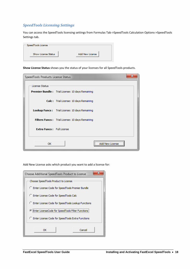
SpeedToolsLicensingSettings
You can access the SpeedTools licensing settings from Formulas Tab‐>SpeedTools Calculation Options‐>SpeedTools
Settings tab.
Show License Status shows you the status of your licenses for all SpeedTools products.
Add New License asks which product you want to add a license for:

FastExcel SpeedTools User Guide Installing and Activating FastExcel SpeedTools 19
And then prompts for the License Activation key.
FastExcel SpeedTools User Guide Getting Started with FastExcel SpeedTools 20
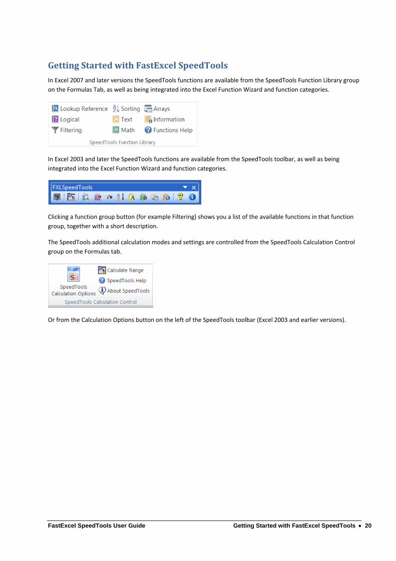
GettingStartedwithFastExcelSpeedTools
In Excel 2007 and later versions the SpeedTools functions are available from the SpeedTools Function Library group
on the Formulas Tab, as well as being integrated into the Excel Function Wizard and function categories.
In Excel 2003 and later the SpeedTools functions are available from the SpeedTools toolbar, as well as being
integrated into the Excel Function Wizard and function categories.
Clicking a function group button (for example Filtering) shows you a list of the available functions in that function
group, together with a short description.
The SpeedTools additional calculation modes and settings are controlled from the SpeedTools Calculation Control
group on the Formulas tab.
Or from the Calculation Options button on the left of the SpeedTools toolbar (Excel 2003 and earlier versions).

FastExcel SpeedTools User Guide SpeedTools Functions 21
SpeedToolsFunctions
FunctionRequirements
Workbooks using the FastExcel SpeedTools functions require that the relevant SpeedTools products are installed
and licensed on the PC that is running the workbooks.
If SpeedTools is installed but not licensed the functions will be available in the Function Wizard and Help, but
will return “# No license found for this Function” to the calling cells.
ExcelFunctionWizard
SpeedToolsFunctionLibrary
Click a function group button on the Formulas Tab (Excel 2007 and later) or the SpeedTools Toolbar (for example
Filtering) to show a list of the available functions in that function group, together with a short description.
You can select a function and choose whether to enter it as an array formula or not. Then clicking OK will enter the
function into the selected cells and launch the Excel Function Wizard.
If the selected cells already contain a formula or data you will be asked if you want to overwrite the existing
information.

FastExcel SpeedTools User Guide SpeedTools Functions 22
NestingSpeedToolsfunctionsusingtheExcelFunctionWizard
If you want to embed SpeedTools functions inside other functions you need to use the Excel Function Wizard
instead of the SpeedTools Function Library Toolbar or Ribbon Group.
In the formula bar select the point in the existing formula where you want to embed the function and click the
Excel Formula wizard button.

FastExcel SpeedTools User Guide SpeedTools Functions 23
ExcelWizardHelp
All the FastExcel SpeedTools functions are available from the Excel Function Wizard. This includes providing a short
description of the function, its arguments and further Help through the Help button on the Function Wizard.
FastExcel SpeedTools User Guide SpeedTools Functions 24
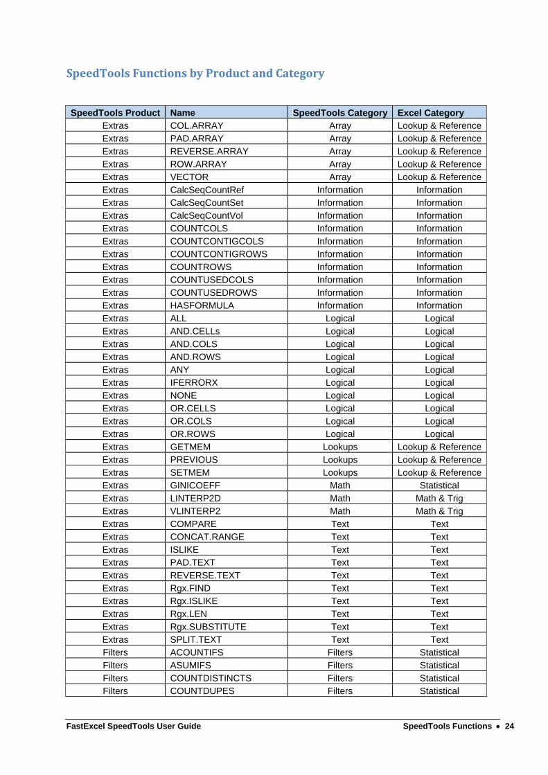
SpeedToolsFunctionsbyProductandCategory
SpeedTools Product Name SpeedTools Category Excel Category Extras COL.ARRAY Array Lookup & Reference
Extras PAD.ARRAY Array Lookup & ReferenceExtras REVERSE.ARRAY Array Lookup & Reference
Extras ROW.ARRAY Array Lookup & ReferenceExtras VECTOR Array Lookup & Reference
Extras CalcSeqCountRef Information Information Extras CalcSeqCountSet Information Information
Extras CalcSeqCountVol Information Information Extras COUNTCOLS Information Information
Extras COUNTCONTIGCOLS Information Information Extras COUNTCONTIGROWS Information Information
Extras COUNTROWS Information Information Extras COUNTUSEDCOLS Information Information
Extras COUNTUSEDROWS Information Information Extras HASFORMULA Information Information
Extras ALL Logical Logical Extras AND.CELLs Logical Logical
Extras AND.COLS Logical Logical Extras AND.ROWS Logical Logical
Extras ANY Logical Logical Extras IFERRORX Logical Logical
Extras NONE Logical Logical Extras OR.CELLS Logical Logical
Extras OR.COLS Logical Logical Extras OR.ROWS Logical Logical
Extras GETMEM Lookups Lookup & ReferenceExtras PREVIOUS Lookups Lookup & Reference
Extras SETMEM Lookups Lookup & ReferenceExtras GINICOEFF Math Statistical
Extras LINTERP2D Math Math & Trig Extras VLINTERP2 Math Math & Trig
Extras COMPARE Text Text Extras CONCAT.RANGE Text Text
Extras ISLIKE Text Text Extras PAD.TEXT Text Text
Extras REVERSE.TEXT Text Text Extras Rgx.FIND Text Text
Extras Rgx.ISLIKE Text Text Extras Rgx.LEN Text Text
Extras Rgx.SUBSTITUTE Text Text Extras SPLIT.TEXT Text Text
Filters ACOUNTIFS Filters Statistical Filters ASUMIFS Filters Statistical
Filters COUNTDISTINCTS Filters Statistical Filters COUNTDUPES Filters Statistical

FastExcel SpeedTools User Guide SpeedTools Functions 25
Filters FILTER.IFS Filters Lookup & ReferenceFilters FILTER.MATCH Filters Lookup & Reference
Filters FILTER.SORTED Filters Lookup & ReferenceFilters FILTER.VISIBLE Filters Lookup & Reference
Filters LISTDISTINCTS Filters Statistical Filters LISTDISTINCTS.AVG Filters Statistical
Filters LISTDISTINCTS.COUNT Filters Statistical Filters LISTDISTINCTS.SUM Filters Statistical
Filters Rgx.COUNTIF Filters Math & Trig Filters Rgx.SUMIF Filters Math & Trig
Filters Case.VSORTC Sorting Math & Trig Filters Case.VSORTC.INDEX Sorting Math & Trig
Filters VSORTB Sorting Math & Trig Filters VSORTB.INDEX Sorting Math & Trig
Filters VSORTC Sorting Math & Trig Filters VSORTC.INDEX Sorting Math & Trig
Lookups AMATCH2 Lookups Lookup & ReferenceLookups AMATCHES2 Lookups Lookup & Reference
Lookups AMATCHNTH Lookups Lookup & ReferenceLookups AVLOOKUP2 Lookups Lookup & Reference
Lookups AVLOOKUPNTH Lookups Lookup & ReferenceLookups AVLOOKUPS2 Lookups Lookup & Reference
Lookups Case.AMATCH2 Lookups Lookup & ReferenceLookups Case.AMATCHES2 Lookups Lookup & Reference
Lookups Case.AMATCHNTH Lookups Lookup & ReferenceLookups Case.AVLOOKUP2 Lookups Lookup & Reference
Lookups Case.AVLOOKUPNTH Lookups Lookup & ReferenceLookups Case.AVLOOKUPS2 Lookups Lookup & Reference
Lookups COMPARE.LISTS Lookups Lookup & ReferenceLookups EVAL Lookups Lookup & Reference
Lookups MEMLOOKUP Lookups Lookup & ReferenceLookups MEMMATCH Lookups Lookup & Reference
Lookups Rgx.AMATCH2 Lookups Lookup & ReferenceLookups Rgx.AMATCHES2 Lookups Lookup & Reference
Lookups Rgx.AMATCHNTH Lookups Lookup & ReferenceLookups Rgx.AVLOOKUP2 Lookups Lookup & Reference
Lookups Rgx.AVLOOKUPNTH Lookups Lookup & ReferenceLookups Rgx.AVLOOKUPS2 Lookups Lookup & Reference
Lookups Rgx.Case.AMATCH2 Lookups Lookup & ReferenceLookups Rgx.Case.AMATCHES2 Lookups Lookup & Reference
Lookups Rgx.Case.AMATCHNTH Lookups Lookup & ReferenceLookups Rgx.Case.AVLOOKUP2 Lookups Lookup & Reference
Lookups Rgx.Case.AVLOOKUPNTH Lookups Lookup & ReferenceLookups Rgx.Case.AVLOOKUPS2 Lookups Lookup & Reference
FastExcel SpeedTools User Guide SpeedTools Functions 26
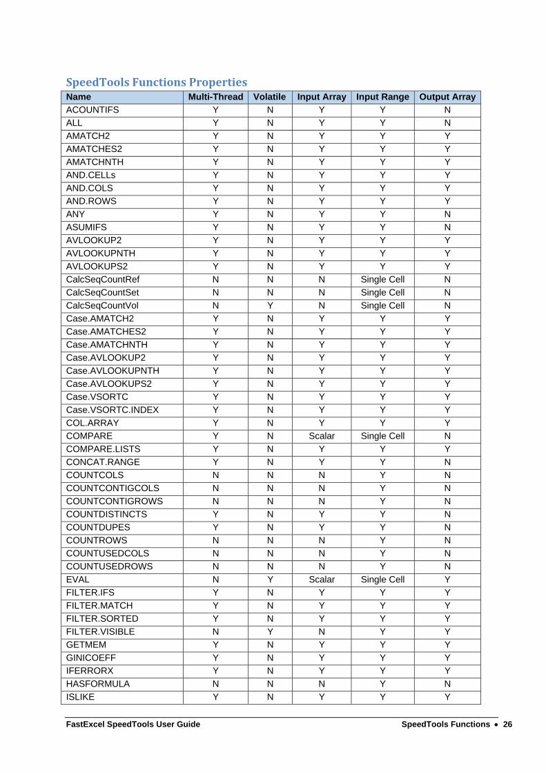
SpeedToolsFunctionsPropertiesName Multi-Thread Volatile Input Array Input Range Output Array
ACOUNTIFS Y N Y Y N
ALL Y N Y Y N
AMATCH2 Y N Y Y Y
AMATCHES2 Y N Y Y Y
AMATCHNTH Y N Y Y Y
AND.CELLs Y N Y Y Y
AND.COLS Y N Y Y Y
AND.ROWS Y N Y Y Y
ANY Y N Y Y N
ASUMIFS Y N Y Y N
AVLOOKUP2 Y N Y Y Y
AVLOOKUPNTH Y N Y Y Y
AVLOOKUPS2 Y N Y Y Y
CalcSeqCountRef N N N Single Cell N
CalcSeqCountSet N N N Single Cell N
CalcSeqCountVol N Y N Single Cell N
Case.AMATCH2 Y N Y Y Y
Case.AMATCHES2 Y N Y Y Y
Case.AMATCHNTH Y N Y Y Y
Case.AVLOOKUP2 Y N Y Y Y
Case.AVLOOKUPNTH Y N Y Y Y
Case.AVLOOKUPS2 Y N Y Y Y
Case.VSORTC Y N Y Y Y
Case.VSORTC.INDEX Y N Y Y Y
COL.ARRAY Y N Y Y Y
COMPARE Y N Scalar Single Cell N
COMPARE.LISTS Y N Y Y Y
CONCAT.RANGE Y N Y Y N
COUNTCOLS N N N Y N
COUNTCONTIGCOLS N N N Y N
COUNTCONTIGROWS N N N Y N
COUNTDISTINCTS Y N Y Y N
COUNTDUPES Y N Y Y N
COUNTROWS N N N Y N
COUNTUSEDCOLS N N N Y N
COUNTUSEDROWS N N N Y N
EVAL N Y Scalar Single Cell Y
FILTER.IFS Y N Y Y Y
FILTER.MATCH Y N Y Y Y
FILTER.SORTED Y N Y Y Y
FILTER.VISIBLE N Y N Y Y
GETMEM Y N Y Y Y
GINICOEFF Y N Y Y Y
IFERRORX Y N Y Y Y
HASFORMULA N N N Y N
ISLIKE Y N Y Y Y
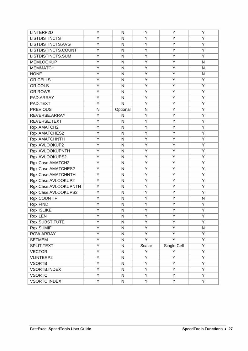
FastExcel SpeedTools User Guide SpeedTools Functions 27
LINTERP2D Y N Y Y Y
LISTDISTINCTS Y N Y Y Y
LISTDISTINCTS.AVG Y N Y Y Y
LISTDISTINCTS.COUNT Y N Y Y Y
LISTDISTINCTS.SUM Y N Y Y Y
MEMLOOKUP Y N Y Y N
MEMMATCH Y N Y Y N
NONE Y N Y Y N
OR.CELLS Y N Y Y Y
OR.COLS Y N Y Y Y
OR.ROWS Y N Y Y Y
PAD.ARRAY Y N Y Y Y
PAD.TEXT Y N Y Y Y
PREVIOUS N Optional N Y Y
REVERSE.ARRAY Y N Y Y Y
REVERSE.TEXT Y N Y Y Y
Rgx.AMATCH2 Y N Y Y Y
Rgx.AMATCHES2 Y N Y Y Y
Rgx.AMATCHNTH Y N Y Y Y
Rgx.AVLOOKUP2 Y N Y Y Y
Rgx.AVLOOKUPNTH Y N Y Y Y
Rgx.AVLOOKUPS2 Y N Y Y Y
Rgx.Case.AMATCH2 Y N Y Y Y
Rgx.Case.AMATCHES2 Y N Y Y Y
Rgx.Case.AMATCHNTH Y N Y Y Y
Rgx.Case.AVLOOKUP2 Y N Y Y Y
Rgx.Case.AVLOOKUPNTH Y N Y Y Y
Rgx.Case.AVLOOKUPS2 Y N Y Y Y
Rgx.COUNTIF Y N Y Y N
Rgx.FIND Y N Y Y Y
Rgx.ISLIKE Y N Y Y Y
Rgx.LEN Y N Y Y Y
Rgx.SUBSTITUTE Y N Y Y Y
Rgx.SUMIF Y N Y Y N
ROW.ARRAY Y N Y Y Y
SETMEM Y N Y Y Y
SPLIT.TEXT Y N Scalar Single Cell Y
VECTOR Y N Y Y Y
VLINTERP2 Y N Y Y Y
VSORTB Y N Y Y Y
VSORTB.INDEX Y N Y Y Y
VSORTC Y N Y Y Y
VSORTC.INDEX Y N Y Y Y

FastExcel SpeedTools User Guide SpeedTools Filters: Filtering Functions 28
SpeedToolsFilters:FilteringFunctionsThe filtering functions provide extended ways of using one or more criteria to filter out subsets of data.
Very fast performance is achieved for sorted data.
The functions can be used within any aggregating function (SUM, MEDIAN, RANK etc.) to provide the
equivalent MEDIANIFS, RANKIFS function.
The functions can also be used as multi‐cell array formula to return the data subsets directly.
ACOUNTIFS ‐ count using extended multiple conditions
ASUMIFS ‐ sum using extended multiple conditions
FILTER.IFS ‐ filter out subsets of data using multiple extended conditions
FILTER.SORTED ‐ filter out subsets of sorted data using multiple extended conditions
FILTER.MATCH ‐ filter out row numbers of the data using multiple extended conditions
FILTER.VISIBLE ‐ filter out the visible rows
Rgx.SUMIF ‐ sum values using Regular Expressions
Rgx.COUNTIF ‐ count values using Regular Expressions
LISTDISTINCTS ‐ provides a list of the distinct rows or cells
LISTDISTINCTS.COUNT ‐ provides a list of the distinct rows or cells, with counts
LISTDISTINCTS.SUM ‐ provides a list of the distinct rows or cells, with sums
LISTDISTINCTS.AVG ‐ provides a list of the distinct rows or cells, with averages
COUNTDISTINCTS ‐ counts the number of distinct rows or cells
COUNTDUPES ‐ counts the number of rows or cells with more than 1 occurrence
FastExcel SpeedTools User Guide SpeedTools Filters: Filtering Functions 29
TheFILTER.IFSMultipleCriteriaFunctionFamily
The FILTER.IFS, FILTER.SORTED, FILTER.MATCH, ASUMIFS and ACOUNTIFS functions are a family of high‐
performance SpeedTools functions you can use to replace many SUMPRODUCT and array functions.
The FILTER.IFS functions are extremely fast when used on sorted data or well‐structured data.
Data can be sorted ascending, descending or unsorted.
Use FILTER.IFS inside functions like RANK, MAX, MIN, SUM, COUNT, COUNTA, AVERAGE, MEDIAN, MODE,
LARGE, INDEX (any function or UDF that will handle a range or array input), or in a multi‐cell array formula
to return the resulting filtered subset of data.
Condition/Criteria operators can be
Relational Operators =, >=, <=, >, <, <>, True, False
~ means Like pattern matching (VBA Like), ~~ means regular expression matching
Data Type Criteria filters #ERR, #TXT, #N, #BOOL, #EMPTY, #ZLS, #TYPE, #BLANK
All Criteria can be inverted using the Not prefix ¬
A list of alternative inclusion or exclusion conditions can be given as an array of Constants or Range
Reference
The Criteria column being compared to the Condition/criteria can be
A column range within or outside the DataRange
A Calculated column range (an expression that evaluates to a column)
An array of Constants
A row is included when ALL of a set of conditions are met.
Sets of Conditions can be separated into #OR# blocks
Columns within the DataRange can be identified either by a label in the first row, or by a column number,
or directly using a range reference.
OptimizingtheperformanceoftheFILTER.IFSfamilyoffunctions
FILTER.IFS is faster with sorted data than unsorted.
FILTER.IFS will exploit grouping or structuring of unsorted data.
The sequence in which the Criteria/Conditions are given can have a significant influence on performance.
Where some criteria apply to the sorted column(s) and some are unsorted, specify the sorted ones first.
For both Sorted and Unsorted data the first criteria should be the one that eliminates the largest number of rows.
For both sorted and unsorted criteria specify = criteria before other types of criteria.

FastExcel SpeedTools User Guide SpeedTools Filters: Filtering Functions 30
Where there are 2 criteria applying to the same column (for example data between 2 dates) the criteria should be adjacent.
For Unsorted data FILTER.IFS will be most efficient when the first criterion results in a relatively small number of groups of row meeting the first criteria
The worst case for FILTER.IFS is unsorted data where the first criterion eliminates every other row.
FastExcel SpeedTools User Guide SpeedTools Filters: Filtering Functions 31
FILTER.IFSfunction
FILTER.IFS returns the cells from the chosen column(s) in the input data range that match the extended conditions
or criteria. The syntax for the criteria is similar to SUMIFS and COUNTIFS but with considerably more options.
FILTER.IFS can be used either to add multiple conditions to aggregating functions like LISTDISTINCTS.SUM, SUM,
MEDIAN, RANK etc. or as a multi‐cell array formula.
FILTER.IFS is most efficient when used with sorted data.
FILTER.IFSSyntax
FILTER.IFS(nsortedCols,InputRange,ReturnCol,CriteriaColumn1,Criteria1,CriteriaColumn2,Criteria2,…,["#OR#",nsortedCols,]CriteriaColumnx,Criteriax,…)
Example: SUM(FILTER.IFS(3,$A$3:$F$10303,"Value","FromCtry","=" & $H6,"ToCtry","=" & $I6,"ToCity","=" & $J6,"Date",">"&$K6,"Date","<"&$L6))
FILTER.IFSParameters
nSortedCols(requiredforalltheFILTER.IFSfamilyfunctionsexceptFILTER.SORTED)
Gives the number of sorted Criteria columns in the InputRange.
If nSortedCols is 2 then CriteriaColumn1 must be the major sort column in the InputRange, CriteriaColumn2 the
next minor sort column in the InputRange, and so on. (In other words InputRange must be sorted by
CriteriaColumn2 within CriteriaColumn1).
The sorted criteria columns must all be sorted Ascending or Descending. Positive nSortedCols indicates sorted
ascending, negative nSortedCols indicates descending and zero indicates that the criteria columns are not sorted.
Columns outside the InputRange and Calculated Columns are always treated as unsorted.
Columns with criteria operators ~, ~~, the Type criteria operators or with a list of criteria given as an array constant
or multi‐cell range reference are always treated as unsorted.
The first column with a criteria operator other than =, True, False will cause subsequent columns to be treated as
unsorted.
Using non‐zero NsortedCols with unsorted data will give unpredictable and usually incorrect results.
InputRange(required)
The reference to the range containing the column from which the subset of results will be returned, and also
containing all the sorted Criteria columns. The InputRange may also contain unsorted Criteria Columns.
The InputRange may optionally contain column labels in the first row, in which case at least one of the criteria
columns or return column should be identified using a label.
ReturnCol(requiredforalltheFILTER.IFSfamilyfunctionsexceptFILTER.MATCH)
Specifies the column in InputRange from which the subset of data will be returned. If given as text will be
interpreted as a column label in the first row of the InputRange. If given as a number will be interpreted as a
column number within InputRange.

FastExcel SpeedTools User Guide SpeedTools Filters: Filtering Functions 32
If ReturnCol is 0 then all the columns in InputRange will be returned (ASUMIFS and ACOUNTIFS return a row of
sums and counts for each column).
CriteriaColumn1(required)
Specifies the first Criteria Column. Can be text, a number, a Range Reference, an array of constants or an
expression that results in a column.
Text will be interpreted as a column label in the first row of the InputRange
Number will be interpreted as a column number within InputRange.
Range Reference will be interpreted as an independent column outside InputRange.
An array of constants will be interpreted as a column of data.
An expression will be evaluated by Excel as a calculated column before being passed to the FILTER function.
If any of the Criteria Columns are calculated columns (contain expressions) then the FILTER function must be
array entered (Control‐Shift‐Enter).
Criteria Columns must contain the same number of rows as the InputRange, but allowance is made for a row of
column labels in either or both the InputRange and Criteria Columns.
Criteria1(required)
Specifies the criteria expression to be applied to CriteraColumn1.
The Criteria expression must resolve to a text string starting with a criteria operator and ending with a Criteria
value.
If no criteria operator is found at the start then = will be assumed.
A Criteria expression may be any Excel expression containing strings, range references, defined names and
operators
CriteriaOperators
Valid Criteria operators are:
The relational operators:
= is equal to
> is greater than
>= is greater than or equal to
< is less than
<= is less than or equal to
¬ is not equal to
If no operator is given it is treated as =, except that the data type is never converted (see Data Types
section below).

FastExcel SpeedTools User Guide SpeedTools Filters: Filtering Functions 33
The Boolean operators:
True the cell value is true
False the cell value is false
The Pattern operators:
~ Like the criteria value pattern using the wild‐card characters * and ?
~~ Matches against a regular expression pattern
Because Excel propagates error values through formulas and expressions the above criteria operators have no
effect when preceding an error value.
The Data Type Operators:
#TYPE the data type of the cell is the same as the first data cell in the criteria column
#ERR the cell contains an error value
#TXT the cell contains a string (text) value
#N the cell contains a number (integer or with decimal point, date, time, currency)
#BOOL the cell contains a Boolean True or False
#EMPTY the cell is empty
#ZLS the cell contains a zero length string
#BLANK the cell contains a string of 1 or more blanks/spaces
Any of these criteria operators can be prefixed by ¬ (not) to convert the operator from an inclusion operator to an
exclusion operator.
DataTypeComparison
Excel has 5 fundamental data types: Number (integers, real numbers, dates, times, currency), String (text), Boolean
(true or false), Error (#NA etc) and Empty (unused cells).
When a column of mixed data types are sorted Excel uses the following comparison relationships:
Numbers < Strings < Booleans < Errors
Empty cells are always sorted last, both in an ascending and a descending sort.
The SpeedTools FILTER functions use the same comparison relationship between data types.
DataTypeConversion
When a criteria value is preceded by any of the criteria operators its data type is not known (Criteria values without
any preceding criteria operator have a specific data type).

FastExcel SpeedTools User Guide SpeedTools Filters: Filtering Functions 34
For example in “<1234” the 1234 could be a number or could be a string. When this criteria value is being
compared to a criteria column that could contain multiple data types the FILTER.IFS functions use the following
rules:
When the criteria operator is ~ or ~~ the criteria value and the values in the criteria column will be converted to
strings before doing the pattern match.
Otherwise the preferred data type will be the data type of the first data (non‐header) cell in the criteria column.
FILTER.IFS will attempt to convert the criteria value to the preferred data type. If this is not possible FILTER.IFS will
convert the criteria value to a number, then a string, then a Boolean then an error.
OverridingDataTypeConversionusingthe&Prefix
If your criteria column contains mixed data types (for instance both numeric and string numbers) you can ask
FILTER.IFS to try to convert the criteria value to the best possible data type match with each cell in the criteria
column.
So FILTER.IFS would use the numeric version of the criteria value to compare with a numeric number and the string
version of the criteria value to compare with a string/text number.
You request this by adding a & character as a prefix to the criteria operator (after the ¬ prefix if you are using the
exclusion prefix).
CriteriaValues
Criteria values and Criteria column values are NOT Case sensitive.

FastExcel SpeedTools User Guide SpeedTools Filters: Filtering Functions 35
CriteriaLikePatterns
Like Patterns can contain:
* Any number of characters, including none
? Any single character
PatternExamples:
Column Value Criteria Result Criteria Explanation
"aBBBa" “~a*a" True String starting with a followed by any characters and ending
with a
“a2a” “~a?a” True String starting with a followed by any single character followed
by a
“BAT123khg" “~B?T*” True B followed by any single character followed by T followed by
any or no characters
“CAT123khg" “~B?T*” False B followed by any single character followed by T followed by
any or no characters

FastExcel SpeedTools User Guide SpeedTools Filters: Filtering Functions 36
CriteriaLists
Criteria can be given either as a single criteria or a list of alternative Criteria.
A list of alternative Criteria can be either an array of Constants or a Range Reference.
The individual elements in the array or cells in the Range Reference may each start with their individual criteria
Operator, or may not have a criteria operator.
If a list of alternative criteria is given it is treated as an OR for each element of the Criteria Column.
If the first element in the list or range is the character ¬ then the list is treated as an exclusion list: values in the
criteria column that match any of the items in the list are excluded from the filter.
CriteriaListsExamples:
FILTER.IFS(0,$A$1:$C$6,"Hundreds","Digits",{"Four","One","Two"},"Tens",{"Fifty","Fourty","Thirty","Twenty"})
The Digits column must contain any of Four, One or Two and the Tens column must contain any of Fifty, Forty,
Thirty or Twenty.
CriteriaColumn2,Criteria2,…(optional)
You can give additional pairs of Criteria Column and Criteria.
All of the Criteria pairs given in a set must be True for a row of data from the Return Column to be included.
"#OR#",nSortedCriteria,(optional)
If you need alternative sets of criteria you can separate them with “#OR#”, nSortedCols.
A row will be selected from the Return Column if ANY of the alternative sets of Criteria are met.
The row will only be selected once if both alternative sets of criteria are met (no double‐counting).
For Example:
CriteriaCol1,Criteria1,CriteriaCol2, Criteria2, “#OR#”,1,CriteriaCol3, Criteria3,CriteriaCol4,Criteria4
A row will be selected from the Return Column if
(both criteria1 and Criteria2 are True) OR (both Criteria3 and Criteria4 are True)
Note that a Criterion can also contain a list of alternative conditions (see above)

FastExcel SpeedTools User Guide SpeedTools Filters: Filtering Functions 37
CombiningFILTER.IFSCriteriainLogicalCombinations
DefaultisAND
By default ALL the criteria given must be met for a row to be included in the subset.
Multiplealternativesforasinglecolumn
You can use criteria lists to give a number of alternative criteria for a single column (OR).
AlternativeSetsofCriteria
Where you have alternative sets of criteria (both Criteria1 and Criteria2 must be True) OR (both Criteria3 and
Criteria4 must be True) you can use #OR# to separate them.
MorecomplexLogicalCombinations
You can use SpeedTools’s OR.ROWS and AND.ROWS functions to build more complicated calculated combinations
of criteria within FILTER (see below).

FastExcel SpeedTools User Guide SpeedTools Filters: Filtering Functions 38
FILTER.IFSExamplesThis example shows how to use FILTER.IFS to filter out data by data type, and how to use ACOUNTIFS to
count the occurrences of each data type.
For the same data here are the results of using the ¬ (NOT) operator with data types.

FastExcel SpeedTools User Guide SpeedTools Filters: Filtering Functions 39
Find the maximum value and total value where month is Feb or June and the ToCity starts with “Oth”.
Show all the rows where FromCtry =AT, month is June, day of the month is >20 and the ToCity starts
with “Oth”

FastExcel SpeedTools User Guide SpeedTools Filters: Filtering Functions 40
FILTER.SORTEDfunction
Filter.Sorted filters out subsets of sorted data using multiple extended conditions.
Use FILTER.SORTED if the first criterion is sorted.
FILTER.SORTEDSyntax
FILTER.SORTED(InputRange,ReturnCol,CriteriaColumn1,Criteria1,CriteriaColumn2,Criteria2,…,["#OR#",nsortedCols,]CriteriaColumnx,Criteriax,…)
See FILTER.IFS for definitions of the parameters for FILTER.SORTED

FastExcel SpeedTools User Guide SpeedTools Filters: Filtering Functions 41
FILTER.MATCHfunction
FILTER.MATCH returns pairs of numbers (1‐based relative position and number of rows) for each contiguous block
of rows that meet the criteria.
FILTER.MATCH should be entered as a 2‐column multi‐row array formula, using Ctrl‐Shift‐Enter.
The first column contains the relative position (first row is 1) within the InputRange of the first row in the block that
meets all the criteria. The second column contains the number of rows in the contiguous block.
The number of pairs returned by FILTER.MATCH is dependent on the data and the criteria being used.
The number pairs can be used by OFFSET to return the block of rows.
FILTER.MATCHSyntax
FILTER.MATCH(nsortedCols,InputRange,CriteriaColumn1,Criteria1,CriteriaColumn2,Criteria2,…,["#OR#",nsortedCols,]CriteriaColumnx,Criteriax,…)
See FILTER.IFS for definitions of the parameters for FILTER.MATCH

FastExcel SpeedTools User Guide SpeedTools Filters: Filtering Functions 42
ASUMIFSfunctionASUMIFS sums the cells in the chosen column(s) that match the extended conditions or criteria.
ASUMIFSSyntax
ASUMIFS(nsortedCols,InputRange,ReturnCol,CriteriaColumn1,Criteria1,CriteriaColumn2,Criteria2,…,["#OR#",nsortedCols,]CriteriaColumnx,Criteriax,…)
ASUMIFS() is equivalent to SUM(FILTER.IFS())
See FILTER.IFS for definitions of the parameters for ASUMIFS.
If ReturnCol is zero then a row of sums will be returned for each column in InputRange, and ASUMIFS should be
entered as a multi‐cell array formula. This is an efficient method of summing multiple columns for a common set of
criteria.

FastExcel SpeedTools User Guide SpeedTools Filters: Filtering Functions 43
ACOUNTIFSfunctionACOUNTIFS counts the cells in the chosen column(s) that match the extended conditions or criteria.
ACOUNTIFSSyntax
ACOUNTIFS(nsortedCols,InputRange,ReturnCol,CriteriaColumn1,Criteria1,CriteriaColumn2,Criteria2,…,["#OR#",nsortedCols,]CriteriaColumnx,Criteriax,…)
ACOUNTIFS() should always be used rather than COUNTA(FILTER.IFS()) because COUNTA counts a return
of zero as 1 but ACOUNTIFS does not.
See FILTER.IFS for definitions of the parameters for ACOUNTIFS
If ReturnCol is zero then a row of counts will be returned for each column in InputRange, and ACOUNTIFS should be
entered as a multi‐cell array formula. This is an efficient method of counting multiple columns for a common set of
criteria.

FastExcel SpeedTools User Guide SpeedTools Filters: Filtering Functions 44
FILTER.VISIBLEfunctionFILTER.VISIBLE returns an array containing all the visible rows in the input Range. Rows that are hidden,
have zero height or are filtered out by AutoFilter are excluded. The input data must be a range.
FILTER.VISIBLE is Volatile, is NOT multithreaded and is an array function.
FILTER.VISIBLESyntax
FILTER.VISIBLE(theRange,Pad)
The first parameter is required, the second is optional.
theRange(Required)
A range reference for the rows and columns to be filtered.
Pad(Optionaldefault#N/A)
The value to use for any excess cells in the array formula. Excess cells are cells in a multi‐cell array
formula that have no corresponding output from the function.
If FILTER.VISIBLE is called from a multi‐cell array formula it will return the smaller of the number of rows
in the multi‐cell array formula or the number of rows in the input range.
If FILTER.VISIBLE is called from a single‐cell array formula it will return the number of rows in the input
range.
FastExcel SpeedTools User Guide SpeedTools Filters: Filtering Functions 45
Rgx.COUNTIFfunction
Counts the number of values within a range or array that match the Regular Expression Pattern.
Rgx.COUNTIF as a multi‐threaded non‐volatile function.
Rgx.COUNTIFSyntax
Rgx.COUNTIF(SearchThis,RegExp,Case_Sensitive)
The first 2 parameters are required; the last parameter is optional.
SearchThis(required)
A rectangular range, array or expression that returns a rectangular array to be searched for matches to the RegEx
Patter. All rows and columns within the rectangular array are evaluated for a match.
RegExp(required)
Specifies the Regular Expression to be used when matching values from SearchThis
Case_Sensitive(optional)
TRUE to make the pattern‐matching case‐sensitive. The default is FALSE.
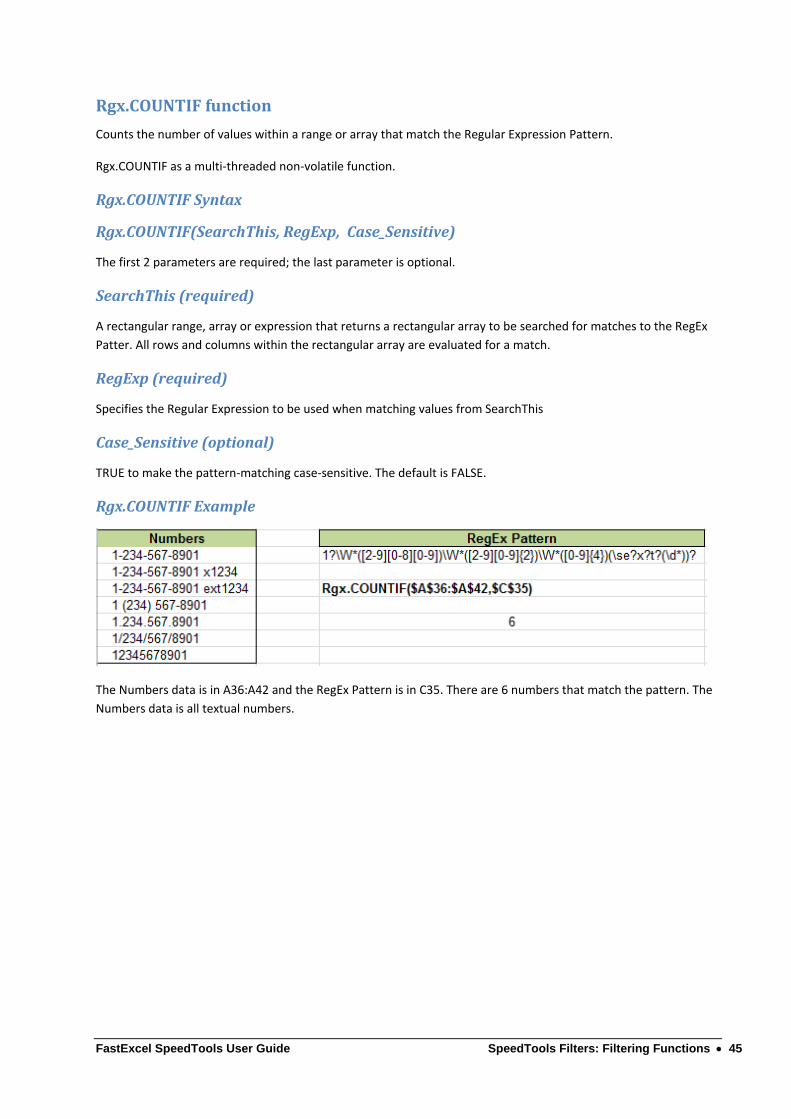
Rgx.COUNTIFExample
The Numbers data is in A36:A42 and the RegEx Pattern is in C35. There are 6 numbers that match the pattern. The
Numbers data is all textual numbers.

FastExcel SpeedTools User Guide SpeedTools Filters: Filtering Functions 46
Rgx.SUMIFfunction
Counts the number of values within a range or array that match the Regular Expression Pattern.
Rgx.SUMIF is a multi‐threaded non‐volatile function.
Rgx.SUMIFSyntax
Rgx.SUMIF(Search_This,RegExp,Sum_This,Case_Sensitive)
The first 2 parameters are required; the last parameter is optional.
Search_This(required)
A rectangular range, array or expression that returns a rectangular array to be searched for matches to the RegEx
Pattern. All rows and columns within the rectangular array are evaluated for a match.
RegExp(required)
Specifies the Regular Expression to be used when matching values from SearchThis
Sum_This(required)
A rectangular range, array or expression that returns a rectangular array that is the same size as Search_This.
Each of the values in positions in Sum_This that correspond to values matched in Search_This will be SUMmed.
Case_Sensitive(optional)
TRUE to make the pattern‐matching case‐sensitive. The default is FALSE.
Rgx.SUMIFExample
The Numbers data is in A36:A42 and the RegEx Pattern is in C35. The Values to be summed are in B36:B42.
There are 6 numbers that match the pattern, and the corresponding values are summed to give 264. The Numbers
data is all textual numbers.
FastExcel SpeedTools User Guide SpeedTools Filters: Filtering Functions 47
TheLISTDISTINCTSfamilyoffunctions.
The 6 functions in the LISTDISTINCTS family provide efficient and flexible methods to work with distinct items or
distinct rows in ranges of data.
The LIST functions are either entered as multi‐cell array formulas using Control/Shift/Enter, or are nested inside
another function that processes the result array. The COUNT functions return a single value and do not need to be
entered as array formulas.
Options are available for:
Case‐sensitivity (Case_Sense)
Distinct Rows (ByRows)
What to show in the unused cells (PadType)
Sorting the output lists (Sort)
Ignoring any combination of error values, blanks or zeros (Ignore)
All of the LISTDISTINCTS functions are multithreaded, non‐volatile array functions.
The Function Wizard category for the LISTDISTINCTS family is Statistical.
The SpeedTools category for the ListDistincts family is Filters.
FastExcel SpeedTools User Guide SpeedTools Filters: Filtering Functions 48
LISTDISTINCTSFunction
LISTDISTINCTS is an array function that returns an array of the distinct cells or row in the input data.
Options control what data will be ignored, case sensitivity, sorting the output and padding the output array.
LISTDISTINCTSSyntax
LISTDISTINCTS(theInputData,Ignore,ByRows,Case_Sense,Sort,PadType)
theInputData
theInputData can be a range or an array of constants or an expression returning an array. It identifies the data to
be searched for distinct items.
Ignore(Optional)
Controls what cell values will be ignored by the distinct test.
1= Error values ignored. 2 = Blanks or Empty Cells ignored. 4 = Zero values ignored. 8 or larger nothing
ignored.
Combinations of Ignore values can be made by adding the values together, although any resulting value
greater than 8 means nothing will be ignored.
Default is 3 =1 & 2
ByRows(Optional)
If theInputData is a range or array with multiple columns and rows you may want either to look for distinct rows of
data or to look for distinct items in all the cells.
If ByRows is specified as True (True is the default) then each row will be checked against all the other rows for
uniqueness. Rows where all the columns contain items to be ignored are not treated as distinct.
If ByRows is False then each cell will be checked against all the other cells for uniqueness. Cells containing items to
be ignored are not treated as distinct.
LISTDISTINCTS.SUM and LISTDISTINCT.AVG always work ByRows
The default for ByRows is TRUE.
Case_Sense(Optional)
Specifies whether the comparison will be made in a case‐sensitive way (Case_Sense=TRUE) or case will be ignored
(Case_Sense=FALSE). The default for Case_Sense is FALSE.
Sort(Optional)
If 0 the output list will be in the same sequence as the theInputData. If 1 the output list of distinct items/rows will
be sorted ascending, or if ‐1 the output list of distinct items/rows will be sorted descending.
For LISTDISTINCTS.COUNT, LISTDISTINCTS.SUM and LISTDISTINCTS.AVG using Sort=2 will sort the column of counts,
sums or averages ascending and Sort=‐2 will sort them descending.
The default for Sort is 0 (unsorted).

FastExcel SpeedTools User Guide SpeedTools Filters: Filtering Functions 49
PadType(Optional‐ArrayHandling)
LISTDISTINCTS.SUM, LISTDISTINCTS.COUNT and LISTDISTINCTS.AVG are array functions that return arrays of
results.
The result arrays can either be used as input to other functions or array formulae, or the functions can be entered
as multi‐cell array formulae so that the result arrays occupy multiple cells.
The functions follow the standard Excel rules for multi‐cell array formulae:
If entered into fewer cells than the result array the excess results are not returned.
If entered into more cells than the result array the excess unused cells will be filled with whatever is specified by PadType (0=#N/A, 1=””, 2=0, default 0=#N/A)
A single‐cell result will be propagated to all the excess unused cells.
A column of results will be propagated to the excess columns
A row of results will be propagated to the excess rows.
COUNTDISTINCTS and COUNTDUPES return a single number, so they do not have a PadType option.
Remarks
COUNTDISTINCTS and COUNTDUPES These functions return a single number: the total number of distinct
items/rows and the total number of duplicated items/rows.
The number of duplicated items/rows is counted as the total count for each non‐ignored distinct item/row ‐1.
They do not need to be entered as array formulae.
LISTDISTINCTS
Unless embedded in another function that will process the array:
If using ByRows the functions should be entered as a multi‐cell array formula with the same number of columns as
theInputData and sufficient rows for each distinct row in theInputData.
If not using ByRows the function should be entered as either a single row or single‐column multi‐cell array formula.
LISTDISTINCTS.COUNT, LISTDISTINCTS.SUM and LISTUNIQUES.AVG
These functions work the same way as LISTUNIQUES except that they produce an extra column containing the
Counts, Sums and Averages respectively.
So make sure to include the extra column when you are entering them as multi‐cell array formulae.
LISTDISTINCTS.SUM and LISTUNIQUES.AVG ignore cells in the SumColumn containing True/False, numbers which
are text and text.

FastExcel SpeedTools User Guide SpeedTools Filters: Filtering Functions 50
LISTDISTINCTS.COUNTFunction
LISTDISTINCTS.COUNT outputs a multi‐column array of the cells or rows from the input data, where the first
column/columns are the distinct items/rows and the last column is the count of that item.
If ByRows is true then the output rows are the distinct rows, but if ByRows is false then the output is 2 columns:
the first column is a list of all the distinct items in the input data and the second column is a count for each distinct
item.
LISTDISTINCTSSyntax
LISTDISTINCTS.COUNT(theInputData,Ignore,ByRows,Case_Sense,Sort,PadType)
See the LISTDISTINCTS function for an explanation of the parameters.
LISTDISTINCTS.COUNT should be entered as a multi‐column multi‐row array formula.

FastExcel SpeedTools User Guide SpeedTools Filters: Filtering Functions 51
LISTDISTINCTS.SUMFunction
LISTDISTINCTS.SUM outputs a multi‐column array of the cells or rows from the input data, where the first
column/columns are the distinct items/rows and the last column is the sum of the SumColumn.
If ByRows is true then the output rows are the distinct rows, but if ByRows is false then the output is 2 columns:
the first column is a list of all the distinct items in the input data and the second column is a sum of the SumColumn
for each distinct item.
LISTDISTINCTS.SUMSyntax
LISTDISTINCTS.SUM(theInputData,SumColumn,Ignore,ByRows,Case_Sense,Sort,PadType)
Parameters apart from SumColumn are explained in the LISTDISTINCTS function.
SumColumn
Can be a range or array of constants or an expression returning an array, and must be arranged as a vertical
column.
The number of rows should be the same as the number of rows in theInputData.
The values for each corresponding distinct row in theInputData will be summed.
LISTDISTINCTS.SUM and LISTUNIQUES.AVG ignore cells in the SumColumn containing True/False, numbers which
are text and text.

FastExcel SpeedTools User Guide SpeedTools Filters: Filtering Functions 52
LISTDISTINCTS.AVGFunction
LISTDISTINCTS.AVG outputs a multi‐column array of the cells or rows from the input data, where the first
column/columns are the distinct items/rows and the last column is the count of that item.
If ByRows is true then the output rows are the distinct rows, but if ByRows is false then the output is 2 columns:
the first column is a list of all the distinct items in the input data and the second column is a average of the
SumColumn for each distinct item.
LISTDISTINCTS.AVGSyntax
LISTDISTINCTS.AVG(theItems,SumColumn,Ignore,ByRows,Case_Sense,Sort,PadType)
Parameters apart from SumColumn are explained in the LISTDISTINCTS function.
SumColumn
Can be a range or array of constants or an expression returning an array, and must be arranged as a vertical
column.
The number of rows should be the same as the number of rows in theInputData.
The values for each corresponding distinct row in theInputData will be averaged.
LISTDISTINCTS.SUM and LISTUNIQUES.AVG ignore cells in the SumColumn containing True/False, numbers which
are text and text.

FastExcel SpeedTools User Guide SpeedTools Filters: Filtering Functions 53
COUNTDISTINCTSFunction
The COUNTDISTINCTS function returns a single number: the total number of distinct items/rows. COUNTDISTINCTS
does not need to be entered as an array formula.
COUNTDISTINCTSSyntax
COUNTDISTINCTS(theInputData,Ignore,ByRows,Case_Sense)
See the LISTDISTINCTS function for an explanation of the parameters.

FastExcel SpeedTools User Guide SpeedTools Filters: Filtering Functions 54
COUNTDUPESFunction
The COUNTDUPES function returns a single number: the total number of duplicated items/rows. COUNTDUPES
does not need to be entered as an array formula.
The number of duplicated items/rows is counted as the total count of items/rows for each non‐ignored distinct
item/row ‐1.
COUNTDUPESSyntax
COUNTDUPES(theInputData,Ignore,ByRows,Case_Sense)
See the LISTDISTINCTS function for an explanation of the parameters

FastExcel SpeedTools User Guide SpeedTools Filters: Filtering Functions 55
LISTDISTINCTSExamples
Sample Data
LISTDISTINCTSArray‐entered6rows,2columns,ByRows
Each distinct row in the input is shown. The extra 2 rows are padded with #N/A.
LISTDISTINCTS.COUNTArrayentered6rows,3cols,ByRows,paddedwithblanks
Each distinct row in the input is shown with a count of the number of occurrences. The extra 2 rows are padded
with blanks.
LISTDISTINCTS.COUNTArrayentered6rows,3cols,ByRows=False,paddedwithblanks
Each distinct item in the Input Data is listed with a count of the number of ocurrences, the extra 2 rows and column
are padded with blanks.

FastExcel SpeedTools User Guide SpeedTools Filters: Filtering Functions 56
LISTDISTINCTS.SUMArrayentered6rows,3cols,paddedwithblanks
The distinct rows are listed with the sum of column E (Spend)
LISTDISTINCTS.AVGArrayentered6rows,3cols,paddedwithblanks
The distinct rows are listed with the average of their Column E Spend.
COUNTDISTINCTByRows.Singlecellformula,NOTarray‐entered
There are 4 distinct rows in A2:B7
COUNTDUPESByRows.Singlecellformula,notarrayentered
There are only 2 duplicates in A2:B7 (2 Rows appear twice)
COUNTDISTINCTByRows=False
There are 6 distinct items in A2:C7

FastExcel SpeedTools User Guide SpeedTools Filters: Filtering Functions 57
LISTDISTINCTByRows=False
The 6 distinct items in A2:C7 are listed
COUNTDUPESByRows=False
There are 12 duplicated items in A2:C7
(3 x Direct, 1 x Retail, 2 x Defense, 2 x Mfg, 1x SpaceCalls, 3 x SuperPhone)
FastExcel SpeedTools User Guide SpeedTools Filters - Sorting Functions 58
SpeedToolsFilters‐SortingFunctionsFastExcel SpeedTools has 6 dynamic sorting functions that can be used to return sorted arrays.
VSORTC ‐ Sort of a vertical range/array, not case sensitive, using Excel’s sorting rules
VSORTC.INDEX ‐ Index sort of a vertical range/array, not case sensitive, using Excel’s sorting rules
Case.VSORTC ‐ Sort of a vertical range/array, case sensitive, lower‐case before upper‐case, using Excel’s sorting rules
Case.VSORTC.INDEX – Index sort of a vertical range/array, case sensitive, lower‐case before upper‐case, using Excel’s sorting rules
VSORTB ‐ Fast sort of a vertical range, case sensitive, upper‐case before lower‐case, ignores collating rules for accented characters
VSORTB.INDEX ‐ Fast Index sort of a vertical range, case sensitive, upper‐case before lower‐case, ignores collating rules for accented characters
The sorting functions use a stable sort method which preserves the original order of equivalent items.
Up to 15 columns in the input data can be sorted using a mixture of ascending and descending sort sequence.
CollatingSequences
A collating sequence defines the order in which characters and values are sorted. Collating sequences
tend to vary by country, and sometimes a given country will have more than one collating sequence
available.
There are 2 different types of text collating sequences available in the FastExcel SpeedTools sorting
functions.
The locale‐dependent collating sequence uses the user‐specified National Language locale sequence.
This handles national characters and character combinations based on the conventions established for
each locale. This is the method used by Excel SORT and all the LOOKUP functions.
The VSORTC, VSORTC.INDEX, Case.VSORTC, Case.VSORTC.INDEX functions all use the locale‐dependent
collating sequence, and follow Excel’s sorting rules for hyphens and apostrophes.
The collating sequence used by VSORTB and VSORTB.INDEX is faster for sorting text than the locale‐
dependent sequence but may not give results compatible with Excel’s SORT and LOOKUP functions using
the sorted option. VSORTB and VSORTB.INDEX ignore Excel’s sorting rules for hyphens and apostrophes.
Excel’s collating sequence by data type is:
Numbers < Textual Numbers < Text < Logical < Error Values < Empty cells (always last)
Empty cells are returned as zero by the SpeedTools sorting functions.

FastExcel SpeedTools User Guide SpeedTools Filters - Sorting Functions 59
SortandIndexSort
A conventional sort returns the input data in sorted order.
An Index Sort returns the position or index in the input data of the nth item in the sort order.
Sort( B, C, A, D) gives A,B,C,D
Index Sort (B, C, A, D) gives 3,1,2,4.
First A is position 3, second B is position 1, third C is position 2, fourth D is position 4.
Case‐SensitiveSort
The locale‐dependent SORTs have both case‐sensitive and case‐insensitive versions. Binary Sorts are
always case‐sensitive:
VSORTC is not case‐sensitive so the relative positions of the equivalent upper and lower case
letters is preserved from the original sequence.
Case.VSORTC is case‐sensitive and sorts lower‐case before upper‐case in the same way as Excel.
VSORTB is also case‐sensitive but sorts upper‐case before lower‐case (this sequence is
dependent on the code‐page and character set being used).

FastExcel SpeedTools User Guide SpeedTools Filters - Sorting Functions 60
VSORTC–DynamictextcollatingSortofaverticalrangeorarrayThis function sorts a vertical array or a range containing one or more columns. The sort is NOT case‐
sensitive and is done using a locale‐based text collating sequence which respects national language
characters. The output sequence will be the same as a non‐case‐sensitive EXCEL SORT.
VSORTC is a non‐volatile multi‐threaded multi‐cell array function.
VSORTCSyntax
VSORTC(theInputData,SortColumn1,SortColumn2,…SortColumn15))
The first parameter is required, all other parameters are optional. The output from VSORTC will be a vertical sorted array. The number of rows sorted and output will be the smaller of the number of rows in the input data, the number of rows in the used range and, if entered as a multi‐cell array formula, the number of rows the function is entered into. The number of columns will be the number of columns in the input data.
TheInputData(required)
The data to be sorted, given as a vertical array of constants or a calculated range or a range. The range or array can
contain as many columns as required.
SortColumn1…SortColumn15(optional)
Gives the index column number(s) of the columns to be used as sort keys. Up to 15 sort keys can be
specified.
Positive column numbers will be sorted ascending and negative column numbers will be sorted
descending. You can have both positive and negative numbers in the same function call. 1 denotes the
first column in the input data. If all Sort Column parameters are omitted all columns in the input data will
be used as ascending sort keys.
VSORTCExamples
VSORTC(A:C) will sort column A to C ascending, using the minimum of the number of rows in the used
range and the number of rows in the multi‐cell array formula that contains VSORTC. If the formula
containing VSORTC is only entered into a single cell then VSORTC will return the number of rows in the
used range.
VSORTC ({4,3,1,2}) returns a single row with 4 columns containing 4,3,1,2 (the input data is a single row).
VSORTC({4;3;1;2}) returns a column with 4 rows containing 1,2,3,4
VSORTC(A1:C100000,1,‐2) will return 100000 rows by 3 columns sorted ascending on column A and descending on column B.

FastExcel SpeedTools User Guide SpeedTools Filters - Sorting Functions 61
Case.VSORTC–Case‐sensitivedynamicSortofaverticalrangeorarrayThis function sorts a vertical array or a range containing one or more columns. The sort IS case‐sensitive
and is done using a locale‐based collating sequence which respects national language characters. The
output sequence will be the same as a case‐sensitive EXCEL SORT.
VSORTC is a non‐volatile multi‐threaded multi‐cell array function.
Case.VSORTCSyntax
Case.VSORTC(theInputData,SortColumn1,SortColumn2,…SortColumn15))
The first parameter is required, all other parameters are optional. The output from Case.VSORTC will be a vertical sorted array. The number of rows sorted and output will be the smaller of the number of rows in the input data, the number of rows in the used range and, if entered as a multi‐cell array formula, the number of rows the function is entered into. The number of columns will be the number of columns in the input data.
TheInputData(required)
The data to be sorted, given as a vertical array of constants or a calculated range or a range. The range or array can
contain as many columns as required.
SortColumn1…SortColumn15(optional)
Gives the index column number(s) of the columns to be used as sort keys. Up to 15 sort keys can be
specified.
Positive column numbers will be sorted ascending and negative column numbers will be sorted
descending. You can have both positive and negative numbers in the same function call. 1 denotes the
first column in the input data.
If all Sort Column parameters are omitted all columns in the input data will be used as ascending sort
keys.
Case.VSORTCExamples
Case.VSORTC(A:C) will sort column A to C ascending, using the minimum of the number of rows in the used range and the number of rows in the multi‐cell array formula that contains Case.VSORTC. If the formula containing Case.VSORTC is only entered into a single cell then Case.VSORTC will return the number of rows in the used range.
Case.VSORTC({B;b;a;A}) returns a column with 4 rows containing a, A, b, B (lower case before upper case).
Case.VSORTC(A1:C100000,1,‐2) will return 100000 rows by 3 columns sorted ascending on column A and descending on column B.

FastExcel SpeedTools User Guide SpeedTools Filters - Sorting Functions 62
VSORTB–FastDynamicSortofaverticalrangeorarrayThis function sorts a vertical array or a range containing one or more columns. The sort is case‐sensitive
and is done using a binary collating sequence which is dependent on the positions of the characters in
the code‐page. The output sequence may NOT be the same as EXCEL SORT for text items.
VSORTB is a non‐volatile multi‐threaded multi‐cell array function.
VSORTBSyntax
VSORTB(theInputData,SortColumn1,SortColumn2,…SortColumn15))
The first parameter is required, all other parameters are optional. The output from VSORTB will be a vertical sorted array. The number of rows sorted and output will be the smaller of the number of rows in the input data, the number of rows in the used range and, if entered as a multi‐cell array formula, the number of rows the function is entered into. The number of columns will be the number of columns in the input data.
TheInputData(required)
The data to be sorted, given as a vertical array of constants or a calculated range or a range. The range or array can
contain as many columns as required.
SortColumn1…SortColumn15(optional)
Gives the index column number(s) of the columns to be used as sort keys. Up to 15 sort keys can be
specified.
Positive column numbers will be sorted ascending and negative column numbers will be sorted
descending. You can have both positive and negative numbers in the same function call.
1 denotes the first column in the input data.
If all Sort Column parameters are omitted all columns in the input data will be used as ascending sort
keys.
VSORTBExamples
VSORTB(A:C) will sort column A to C ascending, using the minimum of the number of rows in the used
range and the number of rows in the multi‐cell array formula that contains VSORTB. If the formula
containing VSORTB is only entered into a single cell then VSORTB will return the number of rows in the
used range.
VSORTB ({4,3,1,2}) returns a single row with 4 columns containing 4,3,1,2 (the input data is a single row).
VSORTB({4;3;1;2}) returns a column with 4 rows containing 1,2,3,4
VSORTB(A1:C100000,1,‐2) will return 100000 rows by 3 columns sorted ascending on column A and descending on column B.

FastExcel SpeedTools User Guide SpeedTools Filters - Sorting Functions 63
VSORTC.INDEX–CollatingTextIndexSortofaverticalrangeorarrayThis function index sorts a vertical array or a range containing one or more columns. The sort is NOT
case‐sensitive and is done using a locale‐based collating sequence which respects national language
characters and Excel’s sorting rules. The output sequence will be the same as a non‐case‐sensitive EXCEL
SORT.
VSORTC.INDEX is a non‐volatile multi‐threaded multi‐cell array function.
VSORTC.INDEXSyntax
VSORTC.INDEX(theInputData,SortColumn1,SortColumn2,…SortColumn15))
The first parameter is required, all other parameters are optional.
The output from VSORTC.INDEX will be a vertical sorted array of index numbers. The index numbers give
the relative position in the input data of the nth item in the sorted output, rather than the sorted output
itself.
The number of rows sorted and output will be the smaller of the number of rows in the input data, the
number of rows in the used range and, if entered as a multi‐cell array formula, the number of rows the
function is entered into. The number of columns will always be 1.
TheInputData(required)
The data to be sorted, given as a vertical array of constants or a calculated range or a range. The range or array can
contain as many columns as required.
SortColumn1…SortColumn15(optional)
Gives the index column number(s) of the columns to be used as sort keys. Up to 15 sort keys can be
specified.
Positive column numbers will be sorted ascending and negative column numbers will be sorted
descending. You can have both positive and negative numbers in the same function call.
1 denotes the first column in the input data.
If all Sort Column parameters are omitted all columns in the input data will be used as ascending sort
keys.
VSORTC.INDEXExamples
VSORTC.INDEX({B;b;a;A}) returns a column with 4 rows containing 3, 4, 1, 2 (first is the 3rd in the
input data (“a”) then the 4th (“A”), then the 1st (“B”), then the 2nd (“b”)) .
VSORTC.INDEX(A1:C100000,1,‐2) will return 100000 rows by 1 column of index numbers sorted
ascending on column A and descending on column B.

FastExcel SpeedTools User Guide SpeedTools Filters - Sorting Functions 64
Case.VSORTC.INDEX–CollatingTextIndexSortofaverticalrangeorarrayThis function index sorts a vertical array or a range containing one or more columns. The sort IS case‐
sensitive and is done using a locale‐based collating sequence which respects national language
characters and Excel’s sorting rules. The output sequence will be the same as a case‐sensitive EXCEL
SORT.
Case.VSORTC.INDEX is a non‐volatile multi‐threaded multi‐cell array function.
Case.VSORTC.INDEXSyntax
Case.VSORTC.INDEX(theInputData,SortColumn1,SortColumn2,…SortColumn15))
The first parameter is required, all other parameters are optional.
The output from Case.VSORTC.INDEX will be a vertical sorted array of index numbers. The index
numbers give the relative position in the input data of the nth item in the sorted output, rather than the
sorted output itself.
The number of rows sorted and output will be the smaller of the number of rows in the input data, the
number of rows in the used range and, if entered as a multi‐cell array formula, the number of rows the
function is entered into. The number of columns will always be 1.
TheInputData(required)
The data to be sorted, given as a vertical array of constants or a calculated range or a range. The range or array can
contain as many columns as required.
SortColumn1…SortColumn15(optional)
Gives the index column number(s) of the columns to be used as sort keys. Up to 15 sort keys can be
specified.
Positive column numbers will be sorted ascending and negative column numbers will be sorted
descending. You can have both positive and negative numbers in the same function call.
1 denotes the first column in the input data.
If all Sort Column parameters are omitted all columns in the input data will be used as ascending sort
keys.
Case.VSORTC.INDEXExamples
Case.VSORTC.INDEX({B;b;a;A}) returns a column with 4 rows containing 3, 4, 2, 1 (first is the 3rd
in the input data (“a”), then the 4th (“A”), then the 2nd (“b” then the 1st (“A”)) (case‐sensitive
collate means lower case before upper case so the a comes before A).
Case.VSORTC.INDEX(A1:C100000,1,‐2) will return 100000 rows by 1 column of index numbers
sorted ascending on column A and descending on column B.

FastExcel SpeedTools User Guide SpeedTools Filters - Sorting Functions 65
VSORTB.INDEX–FastIndexSortofaverticalrangeorarrayThis function index sorts a vertical array or a range containing one or more columns. The sort is case‐
sensitive and is done using a binary collating sequence which is dependent on the positions of the
characters in the code‐page ignoring Excel’s rules for sorting apostrophes and hyphens. The output
sequence may NOT be the same as EXCEL SORT for text items.
VSORTB is a non‐volatile multi‐threaded array function.
VSORTB.INDEXSyntax
VSORTB.INDEX(theInputData,SortColumn1,SortColumn2,…SortColumn15))
The first parameter is required, all other parameters are optional.
The output from VSORTB.INDEX will be a vertical sorted array of index numbers. The index numbers give
the relative position in the input data of the nth item in the sorted output, rather than the sorted output
itself.
The number of rows sorted and output will be the smaller of the number of rows in the input data, the
number of rows in the used range and, if entered as a multi‐cell array formula, the number of rows the
function is entered into. The number of columns will always be 1.
TheInputData(required)
The data to be sorted, given as a vertical array of constants or a calculated range or a range. The range or array can
contain as many columns as required.
SortColumn1…SortColumn15(optional)
Gives the index column number(s) of the columns to be used as sort keys. Up to 15 sort keys can be
specified.
Positive column numbers will be sorted ascending and negative column numbers will be sorted
descending. You can have both positive and negative numbers in the same function call.
1 denotes the first column in the input data.
If all Sort Column parameters are omitted all columns in the input data will be used as ascending sort
keys.
VSORTB.INDEXExamples
VSORTB.INDEX({B;b;a;A}) returns a column with 4 rows containing 3, 4, 2, 1 (first is the 3rd in the
input data (“a”), then the 4th (“A”), then the 2nd (“b” then the 1st (“A”)) (case‐sensitive collate
means lower case before upper case so the a comes before A).
VSORTB.INDEX(A1:C100000,1,‐2) will return 100000 rows by 1 column of index numbers sorted
ascending on column A and descending on column B.

FastExcel SpeedTools User Guide SpeedTools Lookups: Lookup Functions 66
SpeedToolsLookups:LookupFunctions
OutstandingPerformanceSpeedTools Lookups outperforms Excel’s Lookup functions by using better algorithms and efficient C++
multi‐threaded coding:
Exact Match Binary Search
Memory Lookups
Internal Hash tables for List comparisons and array lookups
AdvancedFunctionThe table below shows a summary comparison of the features in Excel and SpeedTools Lookup functions.
Feature Excel VLOOKUP MEMLOOKUP AVLOOKUP family
Sort Default Ascending Not Sorted Not Sorted
Default Match Type Approx Exact Exact
Linear Search Yes Yes Yes
Approx Binary Search Yes No Yes
Exact Binary Search No Yes Yes
Re‐usable Lookup Memory (Row) No Yes Yes
Re‐usable Lookup Memory (Col) No Yes Yes
Re‐usable Lookup Memory (Cell) No Yes Yes
Multi‐Threaded Yes Yes Yes
Horizontal Lookup HLOOKUP Automatic Vertical only
Array, Expression or Range Yes Yes Yes
Lookup Any Column No No Yes
Use Column Labels or Numbers No No Yes
Multiple Lookup Columns (AND) No No Yes
Multiple Lookup Rows (OR) No No Yes
Multiple Answer Columns No No Yes
Return First, Last or Nth Match No No AVLOOKUPNTH
2 Dimensional Lookup INDEX(…,…)) INDEX(…,…) Yes
Return All Matches No No AVLOOKUPS2
No Match Error‐handling IFERROR() IFERROR() Built‐in option
Compare Lists V Slow Faster Super‐Fast (COMPARE.LISTS)
Wild Card Text Match Yes Yes Yes
Case‐Sensitive Match No No Case.AVLOOKUP2
Regular Expression Text Match No No Rgx.AVLOOKUP2…
FastExcel SpeedTools User Guide SpeedTools Lookups: Lookup Functions 67
Better,SaferLookupDefaultsAll the SpeedTools lookup and match functions default to unsorted exact match, since that is the safest
option. Excel’s VLOOKUP and MATCH default to sorted approximate match, which is likely to give
incorrect answers in most cases!
SpeedToolsLookupFamilies
The 27 Lookup functions are organized into families to simplify choosing the particular function best suited to your
needs.
MEMLOOKUP ‐ Fast exact match Lookup using memory
MEMMATCH ‐ Fast exact match MATCH using memory
COMPARE.LISTS ‐ Compares 2 lists to find matching and missing items
AVLOOKUP2 ‐ Fast powerful advanced function lookup
AVLOOKUPS2 ‐ Advanced function lookup returning ALL matches
AVLOOKUPNTH ‐ Advanced function lookup returning the Nth match
AMATCH2 ‐ Fast powerful advanced function MATCH
AMATCHES2 ‐ Advanced function MATCH returning ALL matches
AMATCHNTH ‐ Advanced function MATCHreturning the Nth match
Case.AVLOOKUP2 ‐ Case‐sensitive version of AVLOOKUP2
Case.AVLOOKUPNTH ‐ Case‐sensitive version of AVLOOKUPNTH
Case.AVLOOKUPS2 ‐ Case‐sensitive version of AVLOOKUPS2
Case.AMATCH2 ‐ Case‐sensitive version of AMATCH2
Case.AMATCHES2 ‐ Case‐sensitive version of AMATCHES2
Case.AMATCHNTH ‐ Case‐sensitive version of AMATCHNTH
Rgx.AVLOOKUP2 ‐ Regular Expression version of AVLOOKUP2
Rgx.AVLOOKUPNTH ‐ Regular Expression version of AVLOOKUPNTH
Rgx.AVLOOKUPS2 ‐ Regular Expression version of AVLOOKUPS2
Rgx.AMATCH2 ‐ Regular Expression version of AMATCH2
Rgx.AMATCHES2 ‐ Regular Expression version of AMATCHES2
Rgx.AMATCHNTH ‐ Regular Expression version of AMATCHNTH
Rgx.Case.AVLOOKUP2 ‐ Case‐sensitive version of Rgx.AVLOOKUP2
Rgx.Case.AVLOOKUPNTH ‐ Case‐sensitive version of Rgx.AVLOOKUPNTH
Rgx.Case.AVLOOKUPS2 ‐ Case‐sensitive version of Rgx.AVLOOKUPS2
Rgx.Case.AMATCH2 ‐ Case‐sensitive version of Rgx.AMATCH2
Rgx.Case.AMATCHES2 ‐ Case‐sensitive version of Rgx.AMATCHES2
Rgx.Case.AMATCHNTH ‐ Case‐sensitive version of Rgx.AMATCHNTH

FastExcel SpeedTools User Guide SpeedTools Lookups: Lookup Functions 68
High‐performanceexactmatchMemoryLookups
Written in C++, SpeedTools multi‐threaded Lookup functions provide faster and easy‐to‐use alternatives to Excel’s
MATCH and VLOOKUP functions for exact match lookups on both sorted and unsorted data.
Excel VLOOKUP does exact match lookups by starting at the first row and looking at each row in turn until a match
is found. For large numbers of rows this linear search is slow.
SpeedTools Lookups remember which rows gave a match the last time they were calculated and will try to short‐
circuit the slow linear search by checking the remembered row first. Because Excel has to recalculate Lookups
whenever any of the values in the Lookup Table change (even when the answer does not change) this technique
can provide significant speedups.
For sorted data SpeedTools Lookups uses exact match binary search which is much faster than the exact match
linear search you have to use with Excel lookups.
LookupMemoryisFail‐Safe
If the memory row does NOT give an exact match to the value being looked up then SpeedTools Lookups will do an
exact match linear search or exact match binary search.
FourdifferentkindsofLookupMemory
SpeedTools Lookups can use 4 different kinds of multi‐threaded memory:
Re‐useable Global Memory for Rows or Columns
A single index is stored in global memory for each row (vertical lookups) or column (horizontal lookups).
Global memory is super‐efficient and easy to use because it gets re‐used when you have more than one lookup
formula on the same row looking up different columns in a Table. This global memory works across all worksheets
in all open workbooks.
Book Sheet Row Memory (default option)
If you are using different Lookup Tables on different worksheets but still want to have more than one lookup
formula on a row looking up different columns from the same table you should use this option which stores the
row memory separately for each workbook & worksheet.
Book Sheet Cell Memory
If you are using multiple Lookup Tables formulas on the same sheet and the same row but in different cells you can
use this option which stores the memory separately for each cell.
Named Row Memory within Workbook
If you are using a number of Lookup Tables it may be better to use a separate Named Row Memory for each table.
This allows you to use multiple memory lookup formulas that look up the tables in the same row or even in the
same cell. The named row memory is shared by name across all worksheets within a workbook.
LookupMemoryisstoredwiththeworkbook
All four kinds of Lookup Memory can be stored with the workbook so that it is automatically restored when you
next open the workbook.

FastExcel SpeedTools User Guide SpeedTools Lookups: Lookup Functions 69
ManagingtheGlobalLookupMemorypools
The current Lookup Memory is stored each time the workbook is saved. When a workbook is opened its stored
Lookup Memory is added to the global Lookup Memory pool.
The Lookup Memory Pool persists until the Excel session is closed or Lookup Memory is cleared.
The SpeedTools Settings tab in FastExcel SpeedTools Calculation Options and Settings enables you to control
Lookup Memory.
You can choose whether to save the Lookup Memory and whether to always store it externally to the workbook.
For Excel 2003 and earlier the Lookup Memory is always stored externally. External memory files are stored in the
same directory as the workbook and have file extensions of .mrl, .mcl and .mcs
Clear Memory empties the current Lookup Memory.
Count Lookup Memory gives you a count of each of the three different kinds of Lookup Memory.
Retrieve Memory repopulates the Lookup Memory from the workbook or the external files.
ChoiceofsimpleoradvancedLookupFunctions
MEMMATCH and MEMLOOKUP provide a simple way of replacing your existing exact match VLOOKUP, HLOOKUP,
LOOKUP and MATCH formulas with more efficient memory‐based functions.
MEMMATCH and MEMLOOKUP can accept arrays and calculated ranges for the Lookup_Table, and will do vertical
or horizontal lookups depending on the shape of the Lookup Table.
There an additional 24 Advanced SpeedTools Lookup functions that give you many extended options.

FastExcel SpeedTools User Guide SpeedTools Lookups: Lookup Functions 70
Reconcilinglistssuper‐fastusingCOMPARE.LISTS
If you just want to reconcile 2 lists of items to see where the differences or similarities are you should use
SpeedTools COMPARE.LISTS. This function can count or show you the differences between 2 lists, each with up to a
million rows in Excel 2007 and later, in just a few seconds.
The24AdvancedFunctionLookups
If you need more powerful functions use these advanced Lookup features:
High‐performance multi‐threaded lookups to exploit multiple cores
Written in C++ for ultimate performance
Run with 32 or 64 bit Excel
3 multi‐threaded memory options
Return the first, last or Nth match from multiple answers (does not use lookup memory)
Return all matching answers where duplicates exist in the Lookup Columns to either multi‐cell array formulas or aggregating functions like SUM, AVERAGE, MEDIAN, COUNT etc.
Two‐dimensional Lookup: lookup both rows and columns
Multi‐column Lookup (AND): lookup a row based on more than one column.
Multi‐row Lookup (OR): Allows for multiple rows of lookup values and multiple lookup answers. Use multi‐row Lookups in array formulae or in formulae like SUM, AVERAGE, MEDIAN, COUNT
Use multiple answer columns to return values from multiple columns.
The lookup column(s) can be any column(s) in the Lookup_Table
Specify the Lookup Column(s) and Answer Column(s) using Column header labels or column numbers.
Choice of case‐sensitive or not case‐sensitive matching
Lookups can use regular expressions for text exact match lookup
Lookup_Table can be sorted ascending, descending or not sorted
Lookup_Table can be a range or an array or a calculated range or an expression yielding an array.
Separate Sort and Exact options allow Exact Match with sorted data
Specify the error returned when Exact Match cannot find a matching row
Use wildcard characters * and # in text exact match lookup.

FastExcel SpeedTools User Guide SpeedTools Lookups: Lookup Functions 71
TheAdvancedLookupsFlavors
The advanced LOOKUP functions are combined in a number of different flavors.
AVLOOKUP2 and AMATCH2
Return all matches; return the Nth match and the standard match return.
o For example AMATCHES2, AMATCHNTH, AMATCH2
Case‐sensitive and non‐case‐sensitive
o For example Case.AVLOOKUP2, Case.AVLOOKUPNTH, Case.AVLOOKUPS2
Regular Expression lookup and standard lookup
o For example Rgx.Case.AMATCH2, Rgx.AVLOOKUPS2, Rgx.AMATCHNTH
All combinations of these flavors make 24 different advanced lookup functions in addition to MEMLOOKUP,
MEMMATCH and COMPARE.LISTS.
FastExcel SpeedTools User Guide SpeedTools Lookups: Lookup Functions 72
MEMLOOKUPFunction
The MEMLOOKUP function uses Memory Lookup for faster exact match lookup on both sorted and unsorted data.
Use MEMLOOKUP to replace VLOOKUP, HLOOKUP and LOOKUP.
MEMLOOKUP always does an exact match. On sorted data MEMLOOKUP does an exact match binary search.
If no match is found MEMLOOKUP returns #N/A even with sorted data.
For a vertical range or array MEMLOOKUP looks for a value in the leftmost column of Lookup_Array and then
returns a value in the row where the value was found from a column you specify.
For a horizontal range or array MEMLOOKUP looks for a value in the topmost row of Lookup_Array and then
returns a value in the column where the value was found from a row you specify.
MEMLOOKUP is a multi‐threaded, non‐volatile non‐array function.
MEMLOOKUPSyntax
MEMLOOKUP(Lookup_Value,Lookup_Array,Col_index_num,Sort_Type,MemType_Name,Vertical_Horizontal)
The first 3 parameters are required; the last 4 parameters are optional.
Lookup_Value(required)
Specifies the value to be found in the Lookup_Array. Can be a constant or a range reference or an expression
returning a single value.
Lookup_Array(required)
A vertical or horizontal array of constants, or a range reference or expression, that returns a contiguous rectangular
table of Lookup Values.
Result_Column(required)
For a vertical Lookup_Array the column number or label in the header row in Lookup_Array from which the
matching value should be returned. The first column in Lookup_array is column 1.
For a horizontal Lookup_Array the row number or label in the header column in Lookup_Array from which the
matching value should be returned. The first row in Lookup_array is row 1.
If Result_Column is a string then Lookup_Array is assumed to contain a header row/column to be searched for
Result_Column. If Result_Column cannot be found the function returns an error message “#Result Column not
found in Header”. If Result_Column is a number then Lookup_Array is assumed NOT to contain a header
row/column.

FastExcel SpeedTools User Guide SpeedTools Lookups: Lookup Functions 73
Sort_Type(optional‐default0)
A number 1, 0 or ‐1 indicating the sort sequence of Lookup_Array.
‐1 Sorted Descending
0 Not Sorted
1 Sorted Ascending
The default is 0: not sorted
MemType_Name(Optional,Defaultsto2)
Memory type for lookups can be 0, 1, 2 or 3 or a string that is used as the name for a memory.
3 = Global Memory for Rows or Columns A single index is stored in global memory for each row (vertical
lookups) or column (horizontal lookups).
This global memory is super‐efficient and easy to use when you have more than one lookup formula on
the same row looking up different columns in a Table. This global memory works across all worksheets in
all open workbooks.
2 = Book Sheet Row Memory If you are using different Lookup Tables on different worksheets but still
want to have more than one lookup formula on a row looking up different columns in the same table you
can use this option which stores the row memory separately for each Workbook worksheet.
1 = Book Sheet Cell Memory If you are using multiple Lookup Tables formulas in different cells on the
same sheet and the same row you should use this option which stores the memory separately for each
cell.
0 = Do not use Lookup memory
Named Memory If you give a text string instead of a number it will be used as a named memory. You can
have many named memories in use at the same time (usually one for each Lookup Table). Each named
memory works by row across all sheets within a workbook, so is the best choice when you have:
o More than one memory lookup referring to different lookup tables within a single formula.
o More than one memory lookup referring to different lookup tables in different cells on the same
row, and these lookups are repeated on the same row in multiple sheets.
If this option is not zero, then MEMLOOKUP will first check to see if the index stored in memory that gave the
answer the last time the MEMLOOKUP was calculated still gives the correct answer. If it does then MEMLOOKUP
will return that answer without doing any more processing.
When using Lookup memory and there are multiple exact match answers available MEMLOOKUP will not
necessarily return the answer from the same row as VLOOKUP.
Vertical_Horizontal(Optional,Defaultsto1)
This parameter controls whether the lookup is done vertically or horizontally.

FastExcel SpeedTools User Guide SpeedTools Lookups: Lookup Functions 74
0 = Guess – if the number of rows >= the number of columns vertical, otherwise horizontal
1= Always Vertical (Default)
2= Always Horizontal
MEMLOOKUPPerformance
If your data is unsorted and there is no Lookup Memory already available for the position of the MEMLOOKUP
formula then MEMLOOKUP will do a linear search and store the row or column index found in the Lookup Memory
for subsequent MEMLOOKUP calls.
In this case the second execution of the MEMLOOKUP formula will be much faster than the first.
If your data is sorted then MEMLOOKUP will do an exact match Binary Search, which is very fast, and the second
execution of the MEMLOOKUP formula will also be very fast.

FastExcel SpeedTools User Guide SpeedTools Lookups: Lookup Functions 75
MEMMATCHFunction
The MEMMATCH function uses Memory Lookup for faster exact match lookup on both sorted and unsorted data.
Use MEMMATCH to replace the MATCH function.
MEMMATCH always does an exact match. On sorted data MEMMATCH does an exact match binary search.
If no match is found MEMMATCH returns #N/A even with sorted data.
For a vertical range or array MEMMATCH looks for a value in the leftmost column of Lookup_Array and then
returns the relative position of the item in the Lookup_Array that matches the specified value (Lookup_Value).
For a horizontal range or array MEMMATCH looks for a value in the topmost row of Lookup_Array and then returns
the relative position of the item in the Lookup_Array that matches the specified value (Lookup_Value).
MEMMATCH is a multi‐threaded, non‐volatile, non‐array function.
MEMMATCHSyntax
MEMMATCH(Lookup_Value,Lookup_Array,Col_index_num,Sort_Type,MemType_Name,Vertical_Horizontal)
The first 3 parameters are required; the last 3 parameters are optional.
Lookup_Value(required)
The value to be found in the Lookup_Array. Lookup_Value can be a constant or a range reference or an expression
returning a single value.
Lookup_Array(required)
A vertical or horizontal array of constants, or a range reference or expression, that returns a contiguous rectangular
table of Lookup Values.
Sort_Type(optional‐default0)
A number 1, 0 or ‐1 indicating the sort sequence of Lookup_Array.
‐1 Sorted Descending
0 Not Sorted
1 Sorted Ascending
The default is 0: unsorted

FastExcel SpeedTools User Guide SpeedTools Lookups: Lookup Functions 76
MemType_Name(Optional,Defaultsto2)
Memory type for lookups can be 0, 1, 2 or 3 or a string that is used as the name for a memory.
3 = Global Memory for Rows or Columns A single index is stored in global memory for each row (vertical
lookups) or column (horizontal lookups).
This global memory is super‐efficient and easy to use when you have more than one lookup formula on
the same row looking up different columns in a Table. This global memory works across all worksheets in
all open workbooks.
2 = Book Sheet Row Memory If you are using different Lookup Tables on different worksheets but still
want to have more than one lookup formula on a row looking up different columns in the same table you
can use this option which stores the row memory separately for each Workbook worksheet.
1 = Book Sheet Cell Memory If you are using multiple Lookup Tables formulas in different cells on the
same sheet and the same row you should use this option which stores the memory separately for each
cell.
0 = Do not use Lookup memory
Named Memory If you give a text string instead of a number it will be used as a named memory. You can
have many named memories in use at the same time (usually one for each Lookup Table). Each named
memory works by row across all sheets within a workbook, so is the best choice when you have:
o More than one memory lookup referring to different lookup tables within a single formula.
o More than one memory lookup referring to different lookup tables in different cells on the same
row, and these lookups are repeated on the same row in multiple sheets.
If this option is not zero, then MEMMATCH will first check to see if the index stored in memory that gave the
answer the last time the MEMMATCH was calculated still gives the correct answer. If it does then MEMMATCH will
return that answer without doing any more processing.
When using Lookup memory and there are multiple exact match answers available MEMMATCH will not
necessarily return the answer from the same row as MATCH.
Vertical_Horizontal(Optional,Defaultsto1)
This parameter controls whether the lookup is done vertically or horizontally.
0 = Guess – if the number of rows >= the number of columns vertical, otherwise horizontal
1= Always Vertical (Default)
2= Always Horizontal

FastExcel SpeedTools User Guide SpeedTools Lookups: Lookup Functions 77
MEMMATCHPerformance
If your data is unsorted and there is no Lookup Memory already available for the position of the MEMMATCH
formula then MEMMATCH will do a linear search and store the row or column index found in the Lookup Memory
for subsequent MEMMATCH calls.
In this case the second execution of the MEMMATCH formula will be much faster than the first.
If your data is sorted then MEMMATCH will do an exact match Binary Search, which is very fast, and the second
execution of the MEMMATCH formula will also be very fast.

FastExcel SpeedTools User Guide SpeedTools Lookups: Lookup Functions 78
COMPARE.LISTSFunction
This function does a compare of a LookFor list with a LookIn list. The function is designed to efficiently help you
reconcile two lists of items and find either the items that do match or the items that don’t match.
COMPARE.LISTS is capable of comparing 2 lists, each containing more than a million items, in a small number of
seconds.
COMPARE.LISTS can return:
True/False or “”/”**” for each item in the LookFor list showing whether or not it can be found the LookIn
list.
A count of the items in LookFor NOT FOUND in LookIn
A count of the items in LookFor FOUND in LookIn
A list of the items in LookFor NOT FOUND in LookIn
A list of the items in LookFor FOUND in LookIn
COMPARE.LISTS is a multi‐threaded, non‐volatile array function.
COMPARE.LISTS can handle whole‐column references efficiently.
COMPARE.LISTSSyntax
COMPARE.LISTS(LookFor,LookIn,Output,Case_Sensitive)
The first two parameters are required. The function is designed to be entered either as a multi‐row, single‐column
array formula or as a single‐cell non‐array formula.
LookFor(Required)
A single‐column vertical range or array of data containing the items to be searched for in the LookIn list.
Empty cells in the LookFor list are ignored.
LookIn(Required)
A single‐column vertical range or array of data containing the list of items to be searched for each item in the
LookFor list.
Empty cells in the LookIn list are ignored.
If either of LookFor or LookIn refers to a single empty cell COMPARE.LISTS will return #Value.
Output(Optional:Default=1)
This option controls the type of output returned from COMPARE.LISTS.
Output=1: An array of True/False for each item in the LookFor list showing whether or not it can be found in the
LookIn list.
When using Output=1 enter the COMPARE.LIST function as a multi‐cell array formula alongside the LookFor list so
that you get a corresponding True or False for each item in LookFor.

FastExcel SpeedTools User Guide SpeedTools Lookups: Lookup Functions 79
Output=2: An array of “” or “**” for each item in the LookFor list showing whether or not it can be found the
LookIn list. “**” indicates that the item was not found.
When using Output=2 enter the COMPARE.LIST function as a multi‐cell array formula alongside the LookFor list so
that you get a “” or “**” for each item in LookFor.
Output=3: A Count and list of the items in LookFor that are NOT found in LookIn. The first output cell contains the
count. To get only the count of non‐matching items enter COMPARE.LISTS as a single‐cell non‐array formula.
Output=4: A Count and list of the items in LookFor that ARE found in LookIn. The first output cell contains the
count. To get only the count of matching items enter COMPARE.LISTS as a single‐cell non‐array formula.
Case_Sensitive(Optional:Default=False)
This option controls whether text will be compared case‐sensitively or not. It can be True or False, and the default
value is False so that by default lower‐case text matches upper‐case text.

FastExcel SpeedTools User Guide SpeedTools Lookups: Lookup Functions 80
COMPARE.LISTSExamples
These examples use the following LookIn and LookFor lists
Note: although some of these cells appear empty A15, A16, C13, C16 are not empty,
A8 is empty.
A15 contains a single ‘ character
A16 contains a single space character
C13 contains a single space character
C14 is empty
C16 contains a single ‘ character
OUTPUT=1(Default):TRUE/FALSE
The results in cell D13 and D14 are blank because the empty cells in C13 and C17 have been ignored.
Cells C13 and C16 show TRUE because the LookIn list contains cells with a single space character and a single ‘
character.
Using OUTPUT=1 you can filter the LookFor list for matches, mismatches or empty cells.
OUTPUT=2:**orspace

FastExcel SpeedTools User Guide SpeedTools Lookups: Lookup Functions 81
Using OUTPUT=2 you get ** for each mismatch: this is easier to see than visually scanning for FALSE.
OUTPUT=3and4,single‐cellnon‐arrayformula:
Using OUTPUT=3 as a single‐cell non‐array formula gives you a count of the mismatches. This is useful as a simple
check that everything in the LookFor list can be found in the LookIn list.
Using OUTPUT=4 as a single‐cell non‐array formula gives you a count of the matches.
OUTPUT=3:multi‐cellarrayformula.
This option gives you a count (3 in this case) followed by a list of the mismatches.
Cell F9 shows 35331 which is Excel’s un‐formatted representation of 23/09/1996.
OUTPUT=4:multi‐cellarrayformula

FastExcel SpeedTools User Guide SpeedTools Lookups: Lookup Functions 82
This option gives you a count (7) followed by a list of the matches.
Cell G12 shows #N/A because C15 matches A14.
Note that there are 7 matches listed although you can only see 5:
Cell G11 corresponds to the single space at C13 and is not actually empty.
Cell G13 corresponds to the ‘ character at C16 and is not actually empty.
FastExcel SpeedTools User Guide SpeedTools Lookups: Lookup Functions 83
AVLOOKUP2,AVLOOKUPS2&AVLOOKUPNTHFunctions
Search for values in one or more columns of a table, and return values from the rows where a match is found.
Advanced Lookup functions returning:
either the first value found (AVLOOKUP2)
or all the values found (AVLOOKUPS2)
or the Nth value found (AVLOOKUPNTH)
AVLOOKUP2, AVLOOKUPS2 and AVLOOKUPNTH are NOT case‐sensitive.
The AVLOOKUP functions are multi‐threaded, non‐volatile, array functions.
AVLOOKUPFamilySyntax
AVLOOKUP2(Lookup_Values,Lookup_Table,Answer_Columns,Sorted,Exact_Match,Lookup_Columns,MemType_Name)
The first 3 parameters are required; the last 4 parameters are optional.
AVLOOKUPS2(Lookup_Values,Lookup_Table,Answer_Columns,Sorted,Exact_Match,Lookup_Columns)
The first 3 parameters are required; the last 3 parameters are optional.
AVLOOKUPNTH(Lookup_Values,Lookup_Table,Answer_Columns,Sorted,Exact_Match,Lookup_Columns,Position)
The first 3 parameters are required; the last 4 parameters are optional.
Lookup_Values(required)
The value(s) to be found in the Lookup_Columns.
Can be a single value or multiple values arranged in columns (lookup in multiple lookup columns) and rows (return
multiple answer Rows). A single value can be a constant or a cell reference.
Multiple lookup values can be specified either as an array of constants or as a range referring to multiple cells.
There should be the same number of columns of lookup values as there are columns in the Lookup_Columns.
When doing multi‐column lookups (multiple columns of both lookup values and lookup columns) the AVLOOKUP
functions will look for a row where ALL the lookup values are matched in the corresponding columns (Columns are
treated as AND).
When doing multi‐row lookups (multiple rows of lookup values) the AVLOOKUP functions will look for a row
separately for each row of lookup values (Rows are treated as OR).
A single AVLOOKUP2 or AVLOOKUPNTH statement will return the same number of rows and columns of result
values as there are rows in Lookup_Values and columns in Answer_Columns.
Lookup_Values can contain the wildcard characters ? and * for exact matches on unsorted text data. To find actual
question marks or asterisks add a tilde (~) preceding the character.
Lookup_Table(required)
The rectangular range of cells or array or expression yielding an array to be used for the lookup table. The
array/range must resolve to a single contiguous rectangular array.

FastExcel SpeedTools User Guide SpeedTools Lookups: Lookup Functions 84
Answer_Columns(required)
Specifies the column or columns in Lookup_Table that the AVLOOKUP functions will return values from for the row
or rows that are found in the lookup operation.
Answer_Columns can be a constant, an array of constants, an expression or a reference.
If Answer_Columns evaluates to a number it will be treated as relative column number(s) within Lookup_Table.
If Answer_Columns evaluates to text then the text will be treated as column labels to be found in the first row of Lookup_Table.
If the column labels are not found the AVLOOKUP functions return #REF.
Sorted(optional,defaultstoFalse)
Specifies whether the data in Lookup_Table is sorted on the first Lookup Column ascending, descending or is not
sorted. Valid values for Sorted are:
True, “Asc”, “Yes”, “True”, 1 Ascending
“Des”, ‐1 Descending
False, “No”, 0, any other text Not Sorted
If the Lookup_Table is sorted on the first Lookup_Column the lookup process will be significantly faster.
Exact_Match(optional,defaultstoTrue)
Use this optional parameter when you want the AVLOOKUP functions to find a row in Table_range that exactly
matches the Lookup_Value(s), even with sorted data, and also to specify what to return if an exact match does
not exist.
An exact match will always be done with unsorted data.
A value of False means that an approximate match will be found with sorted data.
Use True to find an exact march with sorted data and return #N/A if not found.
An exact match on sorted data is much more efficient than an exact match on unsorted data.
If a value of anything other than False is specified it will indicate that an exact match is to be done even with
sorted data, and the value given is the value to be returned if no exact match can be found.
If True is specified or the parameter is omitted the error value will be #N/A.
Lookup_Columns(optional,defaultsto1)
Use this optional parameter when you want to control which column(s) in Lookup_Table to use for the lookup.
The default value is 1: the first column in Lookup_Table
If the values are numeric they will be treated as column numbers, if alphabetic they will be treated as column
labels to be found in the first row of Lookup_Table.
If there is more than one column given then there must be a matching set of values given in the columns of
Lookup_Values.
Multiple columns can be given either as an array of constants or as a range reference.
MemType_Name(Optional,Defaultsto2)
Memory type for lookups can be 0, 1, 2 or 3 or a string that is used as the name for a memory.

FastExcel SpeedTools User Guide SpeedTools Lookups: Lookup Functions 85
3 = Global Memory for Rows or Columns A single index is stored in global memory for each row (vertical
lookups) or column (horizontal lookups).
This global memory is super‐efficient and easy to use when you have more than one lookup formula on
the same row looking up different columns in a Table. This global memory works across all worksheets in
all open workbooks.
2 = Book Sheet Row Memory If you are using different Lookup Tables on different worksheets but still
want to have more than one lookup formula on a row looking up different columns in the same table you
can use this option which stores the row memory separately for each Workbook worksheet.
1 = Book Sheet Cell Memory If you are using multiple Lookup Tables formulas in different cells on the
same sheet and the same row you should use this option which stores the memory separately for each
cell.
0 = Do not use Lookup memory
Named Memory If you give a text string instead of a number it will be used as a named memory. You can
have many named memories in use at the same time (usually one for each Lookup Table). Each named
memory works by row across all sheets within a workbook, so is the best choice when you have:
o More than one memory lookup referring to different lookup tables within a single formula.
o More than one memory lookup referring to different lookup tables in different cells on the same
row, and these lookups are repeated on the same row in multiple sheets.
If this option is not zero, then AVLOOKUP2 will first check to see if the index stored in memory that gave the
answer the last time the AVLOOKUP2 was calculated still gives the correct answer. If it does then AVLOOKUP2 will
return that answer without doing any more processing.
When using Lookup memory and there are multiple exact match answers available AVLOOKUP2 will not necessarily
return the answer from the same row as VLOOKUP.
AVLOOKUPS and AVLOOKUPNTH do not use Lookup Memory.
Position(Optional,Defaultsto0,AVLOOKUPNTHonly)
Controls which result will be returned when there are multiple rows that match the Lookup_Values..
N: where N is a positive integer. The Nth match found will be returned
0 : If sorted ascending the largest value that is less than or equal to Lookup_Value If not sorted then the first value found If sorted descending then the smallest value that is greater than or equal to lookup value
‐1: The first value found will always be returned
‐2: the Last Value found will always be returned
‐3: All matches found will be returned
Remarks
AVLOOKUP2 returns the first row that it finds which meets these criteria:
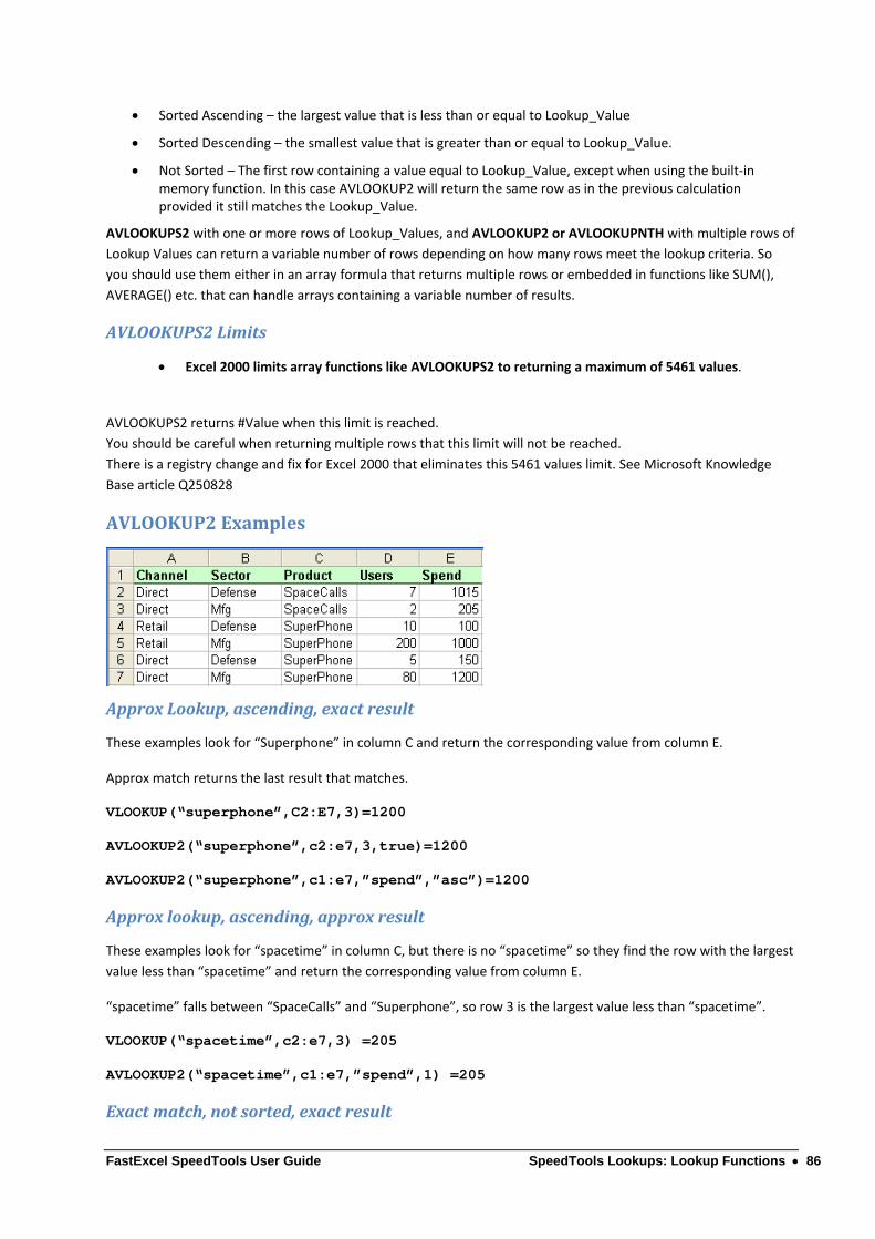
FastExcel SpeedTools User Guide SpeedTools Lookups: Lookup Functions 86
Sorted Ascending – the largest value that is less than or equal to Lookup_Value
Sorted Descending – the smallest value that is greater than or equal to Lookup_Value.
Not Sorted – The first row containing a value equal to Lookup_Value, except when using the built‐in memory function. In this case AVLOOKUP2 will return the same row as in the previous calculation provided it still matches the Lookup_Value.
AVLOOKUPS2 with one or more rows of Lookup_Values, and AVLOOKUP2 or AVLOOKUPNTH with multiple rows of
Lookup Values can return a variable number of rows depending on how many rows meet the lookup criteria. So
you should use them either in an array formula that returns multiple rows or embedded in functions like SUM(),
AVERAGE() etc. that can handle arrays containing a variable number of results.
AVLOOKUPS2Limits
Excel 2000 limits array functions like AVLOOKUPS2 to returning a maximum of 5461 values.
AVLOOKUPS2 returns #Value when this limit is reached.
You should be careful when returning multiple rows that this limit will not be reached.
There is a registry change and fix for Excel 2000 that eliminates this 5461 values limit. See Microsoft Knowledge
Base article Q250828
AVLOOKUP2Examples
ApproxLookup,ascending,exactresult
These examples look for “Superphone” in column C and return the corresponding value from column E.
Approx match returns the last result that matches.
VLOOKUP(“superphone”,C2:E7,3)=1200
AVLOOKUP2(“superphone”,c2:e7,3,true)=1200
AVLOOKUP2(“superphone”,c1:e7,”spend”,”asc”)=1200
Approxlookup,ascending,approxresult
These examples look for “spacetime” in column C, but there is no “spacetime” so they find the row with the largest
value less than “spacetime” and return the corresponding value from column E.
“spacetime” falls between “SpaceCalls” and “Superphone”, so row 3 is the largest value less than “spacetime”.
VLOOKUP(“spacetime”,c2:e7,3) =205
AVLOOKUP2(“spacetime”,c1:e7,”spend”,1) =205
Exactmatch,notsorted,exactresult

FastExcel SpeedTools User Guide SpeedTools Lookups: Lookup Functions 87
These examples look for “superphone” in column C and return the corresponding value from column C. Using
AVLOOKUP2 you can either use the column number or the label of the column (“Spend”). Using the label gives you
much better protection when someone inserts a column between Users and Spend.
Exact match returns the first result that exactly matches.
VLOOKUP(“superphone”,c2:e7,3,false) =100
AVLOOKUP2(“superphone”,c1:e7,”spend”,”No”) =100
ExactMatch,sorted,notfound
This example looks for an exact match to “spacetime” in column C, and cannot find one.
The default value returned if an exact match is not found is #N/A.
VLOOKUP(“spacetime”,c2:e7,3,false) = #N/A
The Sorted parameter is “No” so AVLOOKUP does an exact match and returns the default error #N/A.
AVLOOKUP2(“Spacetime”,C1:E7,”spend”,”No”) = #N/A
AVLOOKUP2 can also do an exact match lookup on sorted data, and it is much faster than an exact match on
unsorted data, particularly with large ranges.
AVLOOKUP2(“Spacetime”,C1:E7,”spend”,”ASC”,True) = #N/A
Gettingridofthe#N/A
If you want to return a value other than #N/A you can use IF tests with either COUNTIF or a double lookup.
IF(COUNTIF(C2:C7,”=spacetime”)=0,”None”, VLOOKUP(“Spacetime”,c2:e7,3,True)) = None
Using AVLOOKUP2 is simpler and faster because it allows you to set the error return value directly and can take
advantage of sorted data.
AVLOOKUP2(“Spacetime”,c1:e7,”spend”,”asc”,”None”) = None
Lookupcolumnnotthefirstcolumn
This example looks for “Superphone” in the “Product” column and returns the corresponding value from the
“Spend” column.
To lookup a column that is not the first column you can use INDEX and MATCH.
INDEX(A2:E7,MATCH(“Superphone”,c2:c7,1),5) = 1200
With AVLOOKUP2 you can specify both the return column and the lookup column directly.
AVLOOKUP2("superphone",A1:E7,"spend",TRUE,FALSE, "product") = 1200

FastExcel SpeedTools User Guide SpeedTools Lookups: Lookup Functions 88
Two‐dimensionallookup
This example looks for “Superphone” in column C and “Spend” in row 1, and returns the value of the intersection
of the row and column found.
You can do a two‐dimensional lookup using INDEX with two MATCH functions.
INDEX(A2:E7,MATCH(“Superphone”,c2:c7,1), MATCH(“Spend”,A1:E1,0)) =1200
AVLOOKUP2 handles two‐dimensional lookups directly.
AVLOOKUP2(“Superphone”,A1:E7,”Spend”,True,False, ”product”) = 1200
Error handling two‐dimensional lookups using INDEX and MATCH is messy.
IF(ISNA(INDEX(A2:E7,MATCH(“superphone”,C2:C7,1), MATCH(“spend”,A1:E1,0))), ”None”,INDEX(A2:E7,MATCH(“superphone”,C2:C7,1), MATCH(“spend”,A1:E1,0))) = 1200
AVLOOKUP2 handles error handling for two‐dimensional lookups directly and much more efficiently.
AVLOOKUP2(“Superphone”,A1:E7,”spend”,”Asc”,”None”,”product”) = 1200
Multicolumnand2Dlookup
This example looks for a row with “superphone” in the “product” column and “defense” in the “sector” column,
and returns the value from the “Users” column. If a row that meets these conditions is not found, AVLOOKUP2
returns “None”.
Looking up multiple columns is simple and efficient with AVLOOKUP2.
AVLOOKUP2({“superphone”,”defense”},A1:E7,”Users”,”Asc”,”None”,{“product”,”sector”}) = 5
The two values to look up and the two columns to look up are specified as arrays using curly brackets. You should
NOT enter this formula as an array formula.
Often it is better to reference ranges that contain the values rather than use arrays. This example assumes that
J34:K34 contains “superphone” and ”defense”, and J33:K33 contains “Product” and “Sector”.
AVLOOKUP2(J34:K34,A1:E7,”Users”,”Asc”,”None”,J33:K33) = 5
UsingRanges,6‐cellarrayformulainD44:E46

FastExcel SpeedTools User Guide SpeedTools Lookups: Lookup Functions 89
This is an example of using AVLOOKUP2 as a multi‐cell array formula. The formula is entered into D44:E46 as an
array formula using Ctrl‐Shift‐Enter, and returns six results because there are three rows to lookup (44:46, each
row has 3 columns to lookup) and two columns (D:E) to return from.
The example looks up “direct” “superphone” and “defense” in the columns labelled “Channel” “product” and
“sector” and returns the values from the corresponding row in columns “Spend” and “Users” (150 and 5). It then
looks up “direct” “superphone” and “mfg” and returns the values 1200 and 80, and finally looks up “retail”
“spacecalls” and “mfg” to return the error values “none” and “none”.
{AVLOOKUP2(A44:C46,A1:E7,D43:E43,"Not","none",A43:C43)}
This multi‐cell array formula is the equivalent of these six individual formulae:
AVLOOKUP2(A44:C44,A1:E7,D43,"Not","none",A43:C43) AVLOOKUP2(A44:C44,A1:E7,E43,"Not","none",A43:C43) AVLOOKUP2(A45:C45,A1:E7,D43,"Not","none",A43:C43) AVLOOKUP2(A45:C45,A1:E7,E43,"Not","none",A43:C43) AVLOOKUP2(A46:C44,A1:E7,D43,"Not","none",A43:C43) AVLOOKUP2(A46:C44,A1:E7,E43,"Not","none",A43:C43)
Note that the sequence of the column names in the Lookup is not the same as the sequence of the column names
in the data.
Returningmultiplerowsandcolumnsusingarraysanda4‐cellarrayformula
You can use arrays of constants or ranges in AVLOOKUP2. In this example the formula is Ctrl‐shift‐entered into
A53:B54.
The first array of lookup values has two rows each containing two lookup values: (comma separates columns,
semicolon separates rows).
The second array {spend, users} specifies the names of the two columns to return values from.
The third array {Product, sector} specifies the names of the two columns to look up.
{AVLOOKUP2({"Superphone","defense";"superphone","mfg"},A1:E7,{"spend","users"},"Asc","None", {"product","sector"})}
The results of the array formula are shown below:
UsingSUMandwildcardswithAVLOOKUPS2
This example uses AVLOOKUPS2 to return all the rows that match a simple lookup for Channel and Sector and a
wildcard lookup for Product. The results are summed separately for Spend and for Users. If no matching rows are
found then 0 will be returned.
D49= SUM(AVLOOKUPS2($A49:$C49,$A$1:$E$7,D$43,"Not",0, $A$43:$C$43))
Fill across to E49 and down to D50:E50

FastExcel SpeedTools User Guide SpeedTools Lookups: Lookup Functions 90
This is NOT an array formula and does not need to be entered using Ctrl‐shift‐Enter.
The answer value of 1405 in D49 is the sum of the Spend column for all the rows that have Channel=Direct and
Sector=Mfg and Product contains a P.
The result of 1405 in D49 comes from the rows returned to SUM as follows:
Row 3: Direct Mfg SpaceCalls = 205
Row 7: Direct Mfg SuperPhone = 1200
The other results are obtained in a similar way.

FastExcel SpeedTools User Guide SpeedTools Lookups: Lookup Functions 91
Case.AVLOOKUP2,Case.AVLOOKUPS2&Case.AVLOOKUPNTHFunctions
Search for values in one or more columns of a table, and return values from the rows where a match is found.
Advanced Lookup functions returning:
either the first value found (Case.AVLOOKUP2)
or all the values found (Case.AVLOOKUPS2)
or the Nth value found (Case.AVLOOKUPNTH)
Case.AVLOOKUP2, Case.AVLOOKUPS2 and Case.AVLOOKUPNTH are case‐sensitive versions of AVLOOKUP2,
AVLOOKUPS2 and AVLOOKUPNTH respectively.
The Case.AVLOOKUP family of functions are multi‐threaded, non‐volatile array functions.
Case.AVLOOKUPFamilySyntax
Case.AVLOOKUP2(Lookup_Values,Lookup_Table,Answer_Columns,Sorted,Exact_Match,Lookup_Columns,MemType_Name)
The first 3 parameters are required; the last 4 parameters are optional.
Case.AVLOOKUPS2(Lookup_Values,Lookup_Table,Answer_Columns,Sorted,Exact_Match,Lookup_Columns)
The first 3 parameters are required; the last 3 parameters are optional.
Case.AVLOOKUPNTH(Lookup_Values,Lookup_Table,Answer_Columns,Sorted,Exact_Match,Lookup_Columns,Position)
The first 3 parameters are required; the last 4 parameters are optional.
Lookup_Values(required)
The value(s) to be found in the Lookup_Columns.
Can be a single value or multiple values arranged in columns (lookup in multiple lookup columns) and rows (return
multiple answer Rows).
A single value can be a constant or a cell reference.
Multiple lookup values can be specified either as an array of constants or as a range referring to multiple cells.
There should be the same number of columns of lookup values as there are columns in the Lookup_Columns.
When doing multi‐column lookups (multiple columns of both lookup values and lookup columns) the
Case.AVLOOKUP functions will look for a row where ALL the lookup values are matched in the corresponding
columns (Columns are treated as AND).
When doing multi‐row lookups (multiple rows of lookup values) the Case.AVLOOKUP functions will look for a row
separately for each row of lookup values (Rows are treated as OR).
A single Case.AVLOOKUP2 or Case.AVLOOKUPNTH statement will return the same number of rows and columns of
result values as there are rows in Lookup_Values and columns in Answer_Columns.
Lookup_Values can contain the wildcard characters ? and * for exact matches on unsorted text data. To find actual
question marks or asterisks add a tilde (~) preceding the character.

FastExcel SpeedTools User Guide SpeedTools Lookups: Lookup Functions 92
Lookup_Table(required)
The rectangular range of cells or array or expression yielding an array to be used for the lookup table. The
array/range must resolve to a single contiguous rectangular array.
Answer_Columns(required)
Specifies the column or columns in Lookup_Table that the Case.AVLOOKUP functions will return values from for the
row or rows that are found in the lookup operation.
Answer_Columns can be a constant, an array of constants, an expression or a reference.
If Answer_Columns evaluates to a number it will be treated as relative column number(s) within Lookup_Table.
If Answer_Columns evaluates to text then the text will be treated as column labels to be found in the first row of Lookup_Table.
If the column labels are not found the Case.AVLOOKUP functions return #REF.
Sorted(Optional,defaultFalse)
Specifies whether the data in Lookup_Table is sorted on the first Lookup Column ascending, descending or not
sorted. Valid values for Sorted are:
True, “Asc”, “Yes”, “True”, 1 Ascending
“Des”, ‐1 Descending
False, “No”, 0, any other text Not Sorted
If the Lookup_Table is sorted on the first Lookup_Column the lookup process will be significantly faster.
Exact_Match(optional,defaultstoTrue)
Use this optional parameter when you want the Case.AVLOOKUP functions to find a row in Table_range that
exactly matches the Lookup_Value(s), even with sorted data, and also to specify what to return if an exact match
does not exist.
An exact match will always be done with unsorted data.
A value of False means that an approximate match will be found with sorted data.
Use True to find an exact march with sorted data and return #N/A if not found.
An exact match on sorted data is much more efficient than an exact match on unsorted data.
If a value of anything other than False is specified it will indicate that an exact match is to be done even with
sorted data, and the value given specifies the value to be returned if no exact match can be found.
If True is specified or the parameter is omitted the error value will be #N/A.
Lookup_Columns(optional,defaultsto1)
Use this optional parameter when you want to control which column(s) in Lookup_Table to use for the lookup.
The default value is 1: the first column in Lookup_Table.
If the values are numeric they will be treated as column numbers, if alphabetic they will be treated as column
labels to be found in the first row of Lookup_Table.
If there is more than one column given then there must be a matching set of values given in the columns of
Lookup_Values.

FastExcel SpeedTools User Guide SpeedTools Lookups: Lookup Functions 93
Multiple columns can be given either as an array of constants or as a range reference.
MemType_Name(Optional,Defaultsto2)
Memory type for lookups can be 0, 1, 2 or 3 or a string that is used as the name for a memory.
3 = Global Memory for Rows or Columns A single index is stored in global memory for each row (vertical lookups) or column (horizontal lookups). This global memory is super‐efficient and easy to use when you have more than one lookup formula on the same row looking up different columns in a Table. This global memory works across all worksheets in all open workbooks.
2 = Book Sheet Row Memory If you are using different Lookup Tables on different worksheets but still want to have more than one lookup formula on a row looking up different columns in the same table you can use this option which stores the row memory separately for each Workbook worksheet.
1 = Book Sheet Cell Memory If you are using multiple Lookup Tables formulas in different cells on the same sheet and the same row you should use this option which stores the memory separately for each cell.
0 = Do not use Lookup memory
Named Memory If you give a text string instead of a number it will be used as a named memory. You can have many named memories in use at the same time (usually one for each Lookup Table). Each named memory works by row across all sheets within a workbook, so is the best choice when you have:
o More than one memory lookup referring to different lookup tables within a single formula.
o More than one memory lookup referring to different lookup tables in different cells on the same row, and these lookups are repeated on the same row in multiple sheets.
If this option is not zero, then Case.AVLOOKUP2 will first check to see if the index stored in memory that gave the
answer the last time the Case.AVLOOKUP2 was calculated still gives the correct answer. If it does then
Case.AVLOOKUP2 will return that answer without doing any more processing.
When using Lookup memory and there are multiple exact match answers available Case.AVLOOKUP2 will not
necessarily return the answer from the same row as VLOOKUP.
Case.AVLOOKUPS and Case.AVLOOKUPNTH do not use Lookup Memory.
Position(Optional,Defaultsto0,Case.AVLOOKUPNTHonly)
Controls which result will be returned when there are multiple rows that match the Lookup_Values..
N: where N is a positive integer. The Nth match found will be returned
0 : If sorted ascending the largest value that is less than or equal to Lookup_Value If not sorted then the first value found If sorted descending then the smallest value that is greater than or equal to lookup value
‐1: The first value found will always be returned
‐2: the Last Value found will always be returned
‐3: All matches found will be returned
Remarks
Case.AVLOOKUP2 returns the first row that it finds which meets these criteria:

FastExcel SpeedTools User Guide SpeedTools Lookups: Lookup Functions 94
Sorted Ascending – the largest value that is less than or equal to Lookup_Value
Sorted Descending – the smallest value that is greater than or equal to Lookup_Value.
Not Sorted – The first row containing a value equal to Lookup_Value, except when using the built‐in memory function. In this case Case.AVLOOKUP2 will return the same row as in the previous calculation provided it still matches the Lookup_Value.
Case.AVLOOKUPS2 with one or more rows of Lookup_Values, and Case.AVLOOKUP2 or Case.AVLOOKUPNTH with
multiple rows of Lookup Values can return a variable number of rows depending on how many rows meet the
lookup criteria. So you should use them either in an array formula that returns multiple rows or embedded in
functions like SUM(), AVERAGE() etc. that can handle arrays containing a variable number of results.
Case.AVLOOKUPS2Limits
Excel 2000 limits array functions like Case.AVLOOKUPS2 to returning a maximum of 5461 values.
Case.AVLOOKUPS2 returns #Value when this limit is reached.
You should be careful when returning multiple rows that this limit will not be reached.
There is a registry change and fix for Excel 2000 that eliminates this 5461 values limit. See Microsoft Knowledge
Base article Q250828

FastExcel SpeedTools User Guide SpeedTools Lookups: Lookup Functions 95
AMATCH2,AMATCHES2&AMATCHNTHfunctions
Search for values in one or more columns of a table, and return the relative position of the row(s) where a match is
found.
Advanced MATCH functions returning:
either the relative position of the first value found (AVMATCH2)
or the relative position of all the values found (AVMATCHES2)
or the relative position of the Nth value found (AMATCHNTH)
These functions are similar to the AVLOOKUP2, AVLOOKUPS2 and AVLOOKUPNTH functions except that they return
relative row numbers rather than values.
These functions are NOT case‐sensitive.
The AMATCH functions are multi‐threaded, non‐volatile array functions.
AMATCHFamilySyntax
AMATCH2(Lookup_Values,Lookup_Table,Sorted,Exact_Match,Lookup_Columns,MemType_Name)
The first 2 parameters are required; the last 4 parameters are optional.
AMATCHES2(Lookup_Values,Lookup_Table,Sorted,Exact_Match,Lookup_Columns)
The first 2 parameters are required; the last 3 parameters are optional.
AMATCHNTH(Lookup_Values,Lookup_Table,Sorted,Exact_Match,Lookup_Columns,Position)
The first 2 parameters are required; the last 4 parameters are optional.
AMATCH2, AMATCHES2 and AMATCHNTH return row number(s) within the range specified by Lookup_Table.
Lookup_Values(required)
Specifies the value(s) to be found in the Lookup_Columns. Can be a single value or multiple values arranged in
columns (multiple lookup columns) and rows (multiple Lookup Rows).
A single value can be a constant or a range reference.
Multiple lookup values can be specified either as an array of constants or as a range referring to multiple cells.
There should be the same number of columns of lookup values as there are columns in the Lookup_Columns.
When doing multi‐column lookups (multiple columns of both lookup values and lookup columns) the AMATCH
functions will look for a row where ALL the lookup values are matched in the corresponding columns (Columns are
treated as AND).
When doing multi‐row lookups (multiple rows of lookup values) the AMATCH functions will look for a row
separately for each row of lookup values (Rows are treated as OR).
A single AMATCH2 or AMATCHNTH statement will return the same number of row numbers as there are rows in
Lookup_Values.

FastExcel SpeedTools User Guide SpeedTools Lookups: Lookup Functions 96
Lookup_Values can contain the wildcard characters ? and * for exact matches on unsorted text data. To find actual
question marks or asterisks add a tilde (~) preceding the character.
Lookup_Table(required)
The rectangular range of cells or array or expression yielding an array to be used for the lookup table. The
array/range must resolve to a single contiguous rectangular array.
Sorted(Optional,defaultstoFalse)
Specifies whether the data in Lookup_Table is sorted on the first Lookup Column ascending, descending or not
sorted. Valid values for Sorted are:
True, “Asc”, “Yes”, “True”, 1 Ascending
“Des”, ‐1 Descending
False, “No”, 0, any other text Not Sorted
If the Lookup_Table is sorted on the first Lookup_Column the lookup process will be significantly faster.
Exact_Error(optional,defaultstoTrue)
Use this optional parameter when you want the AMATCH functions to find a row in Lookup_Table that exactly
matches the Lookup_Value(s), even with sorted data, and to specify what to return if an exact match does not
exist.
An exact match will always be done with unsorted data.
A value of False means that an approximate match will be found with sorted data.
Use True to find an exact march with sorted data and return #N/A if not found.
An exact match on sorted data is much more efficient than an exact match on unsorted data.
If a value of anything other than False is specified it will indicate that an exact match is to be done even with sorted
data, and the value given specifies the value to be returned if no exact match can be found.
If True is specified or the parameter is omitted the error value will be #N/A.
Lookup_Columns(optional,defaultsto1)
Use this optional parameter when you want to control which column(s) in Lookup_Table to use for the lookup.
The default value is 1: the first column in Lookup_Table
If the values are numeric they will be treated as column numbers, if alphabetic they will be treated as column
labels to be found in the first row of Lookup_Table.
If there is more than one column given then there must be a matching set of values given in the columns of
Lookup_Values.
Multiple columns can be given either as an array of constants or as a range reference.
MemType_Name(Optional,Defaultsto2)
Memory type for lookups can be 0, 1, 2 or 3 or a string that is used as the name for a memory.

FastExcel SpeedTools User Guide SpeedTools Lookups: Lookup Functions 97
3 = Global Memory for Rows or Columns A single index is stored in global memory for each row (vertical
lookups) or column (horizontal lookups).
This global memory is super‐efficient and easy to use when you have more than one lookup formula on
the same row looking up different columns in a Table. This global memory works across all worksheets in
all open workbooks.
2 = Book Sheet Row Memory If you are using different Lookup Tables on different worksheets but still
want to have more than one lookup formula on a row looking up different columns in the same table you
can use this option which stores the row memory separately for each Workbook worksheet.
1 = Book Sheet Cell Memory If you are using multiple Lookup Tables formulas in different cells on the
same sheet and the same row you should use this option which stores the memory separately for each
cell.
0 = Do not use Lookup memory
Named Memory If you give a text string instead of a number it will be used as a named memory. You can
have many named memories in use at the same time (usually one for each Lookup Table). Each named
memory works by row across all sheets within a workbook, so is the best choice when you have:
o More than one memory lookup referring to different lookup tables within a single formula.
o More than one memory lookup referring to different lookup tables in different cells on the same
row, and these lookups are repeated on the same row in multiple sheets.
If this option is not zero, then AMATCH2 will first check to see if the index stored in memory that gave the answer
the last time the AMATCH2 was calculated still gives the correct answer. If it does then AMATCH2 will return that
answer without doing any more processing.
When using Lookup memory and there are multiple exact match answers available AMATCH2 will not necessarily
return the answer from the same row as MATCH.
AMATCHES2 and AMATCHNTH do not use lookup memory.
Position(Optional,Defaultsto0,AMATCHNTHonly)
Controls which result will be returned from multiple matches.
N: where N is a positive integer. The Nth match found will be returned
0 : If sorted ascending then the largest value that is less than or equal to Lookup_Value If not sorted then the first value found If sorted descending then the smallest value that is greater than or equal to lookup value
‐1: The first value found will always be returned
‐2: the Last Value found will always be returned
‐3: All matches found will be returned
Remarks
AMATCH2 returns the first row number that it finds which meets these criteria:
FastExcel SpeedTools User Guide SpeedTools Lookups: Lookup Functions 98
Sorted Ascending – the largest value that is less than or equal to Lookup_Value
Sorted Descending – the smallest value that is greater than or equal to Lookup_Value.
Not Sorted – The first row containing a value equal to Lookup_Value, except when using the built‐in memory function. In this case AMATCH2 will return the same row as in the previous calculation provided it still matches the Lookup_Value.
AMATCHES2 with one or more rows of Lookup_Values, and AMATCH2 or AMATCHNTH with multiple rows of
Lookup Values can return a variable number of rows depending on how many rows meet the lookup criteria. So
you should use them either in an array formula that returns multiple rows or embedded in functions like SUM(),
AVERAGE() etc. that can handle arrays containing a variable number of results.
AMATCH2andAMATCHES2Limits
Excel 2000 limit array functions like AMATCH to returning a maximum of 5461 values.
AMATCHES2 returns #Value when this limit is reached.
You should be careful when returning multiple matches that this limit will not be reached.
There is a registry change and fix for Excel 2000 that eliminates this 5461 values limit. See Microsoft Knowledge
Base article Q250828
FastExcel SpeedTools User Guide SpeedTools Lookups: Lookup Functions 99
Case.AMATCH2,Case.AMATCHES2&Case.AMATCHNTHfunctions
Search for values in one or more columns of a table, and return the relative position of the row(s) where a match is
found.
Advanced MATCH functions returning:
either the relative position of the first value found (Case.AMATCH2)
or the relative position of all the values found (Case.AMATCHES2)
or the relative position of the Nth value found (Case.AMATCHNTH)
These functions are similar to the Case.AVLOOKUP2, Case.AVLOOKUPS2 and Case.AVLOOKUPNTH functions except
that they return relative row numbers rather than values.
These functions are case‐sensitive versions of AMATCH2, AMATCHES2 and AMATCHNTH
The Case.AMATCH functions are multi‐threaded, non‐volatile array functions.
Case.AMATCHFamilySyntax
Case.AMATCH2(Lookup_Values,Lookup_Table,Sorted,Exact_Match,Lookup_Columns,MemType_Name)
The first 2 parameters are required; the last 4 parameters are optional.
Case.AMATCHES2(Lookup_Values,Lookup_Table,Sorted,Exact_Match,Lookup_Columns)
The first 2 parameters are required; the last 3 parameters are optional.
Case.AMATCHNTH(Lookup_Values,Lookup_Table,Sorted,Exact_Match,Lookup_Columns,Position)
The first 2 parameters are required; the last 4 parameters are optional.
Case.AMATCH2, Case.AMATCHES2 and Case.AMATCHNTH return the relative position of row(s) within the range
specified by Lookup_Table.
Lookup_Values(required)
Specifies the value(s) to be found in the Lookup_Columns. Can be a single value or multiple values arranged in
columns (multiple lookup columns) and rows (multiple Lookup Rows).
A single value can be a constant or a range reference.
Multiple lookup values can be specified either as an array of constants or as a range referring to multiple cells.
There should be the same number of columns of lookup values as there are columns in the Lookup_Columns.
When doing multi‐column lookups (multiple columns of both lookup values and lookup columns) the Case.AMATCH
functions will look for a row where ALL the lookup values are matched in the corresponding columns (Columns are
treated as AND).
When doing multi‐row lookups (multiple rows of lookup values) the Case.AMATCH functions will look for a row
separately for each row of lookup values (Rows are treated as OR).
A single Case.AMATCH2 or CaseAMATCHNTH statement will return the same number of row numbers as there are
rows in Lookup_Values.

FastExcel SpeedTools User Guide SpeedTools Lookups: Lookup Functions 100
Lookup_Values can contain the wildcard characters ? and * for exact matches on unsorted text data. To find actual
question marks or asterisks add a tilde (~) preceding the character.
Lookup_Table(required)
The rectangular range of cells or array or expression yielding an array to be used for the lookup table. The
array/range must resolve to a single contiguous rectangular array.
Sorted(Optional,defaultstoFalse)
Specifies whether the data in Lookup_Table is sorted on the first Lookup Column ascending, descending or not
sorted. Valid values for Sorted are:
True, “Asc”, “Yes”, “True”, 1 Ascending
“Des”, ‐1 Descending
False, “No”, 0, any other text Not Sorted
If the Lookup_Table is sorted on the first Lookup_Column the lookup process will be significantly faster.
Exact_Error(optional,defaultstoTrue)
Use this optional parameter when you want the Case.AMATCH functions to find a row in Lookup_Table that exactly
matches the Lookup_Value(s), even with sorted data, and to specify what to return if an exact match does not
exist.
An exact match will always be done with unsorted data.
A value of False means that an approximate match will be found with sorted data.
Use True to find an exact march with sorted data and return #N/A if not found.
An exact match on sorted data is much more efficient than an exact match on unsorted data.
If a value of anything other than False is specified it will indicate that an exact match is to be done even with sorted
data, and the value given specifies the value to be returned if no exact match can be found.
If True is specified or the parameter is omitted the error value will be #N/A.
Lookup_Columns(optional,defaultsto1)
Use this optional parameter when you want to control which column(s) in Lookup_Table to use for the lookup.
The default value is 1: the first column in Lookup_Table
If the values are numeric they will be treated as column numbers, if alphabetic they will be treated as column
labels to be found in the first row of Lookup_Table.
If there is more than one column given then there must be a matching set of values given in the columns of
Lookup_Values.
Multiple columns can be given either as an array of constants or as a range reference.
MemType_Name(Optional,Defaultsto2)
Memory type for lookups can be 0, 1, 2 or 3 or a string that is used as the name for a memory.

FastExcel SpeedTools User Guide SpeedTools Lookups: Lookup Functions 101
3 = Global Memory for Rows or Columns A single index is stored in global memory for each row (vertical
lookups) or column (horizontal lookups).
This global memory is super‐efficient and easy to use when you have more than one lookup formula on
the same row looking up different columns in a Table. This global memory works across all worksheets in
all open workbooks.
2 = Book Sheet Row Memory If you are using different Lookup Tables on different worksheets but still
want to have more than one lookup formula on a row looking up different columns in the same table you
can use this option which stores the row memory separately for each Workbook worksheet.
1 = Book Sheet Cell Memory If you are using multiple Lookup Tables formulas in different cells on the
same sheet and the same row you should use this option which stores the memory separately for each
cell.
0 = Do not use Lookup memory
Named Memory If you give a text string instead of a number it will be used as a named memory. You can
have many named memories in use at the same time (usually one for each Lookup Table). Each named
memory works by row across all sheets within a workbook, so is the best choice when you have:
o More than one memory lookup referring to different lookup tables within a single formula.
o More than one memory lookup referring to different lookup tables in different cells on the same
row, and these lookups are repeated on the same row in multiple sheets.
If this option is not zero, then Case.AMATCH2 will first check to see if the index stored in memory that gave the
answer the last time the Case.AMATCH2 was calculated still gives the correct answer. If it does then
Case.AMATCH2 will return that answer without doing any more processing.
When using Lookup memory and there are multiple exact match answers available Case.AMATCH2 will not
necessarily return the answer from the same row as MATCH.
Case.AMATCHES2 and Case.AMATCHNTH do not use lookup memory.
Position(Optional,Defaultsto0,Case.AMATCHNTHonly)
Controls which result will be returned from multiple matches.
N: where N is a positive integer. The Nth match found will be returned
0 : If sorted ascending the largest value that is less than or equal to Lookup_Value If not sorted then the first value found If sorted descending then the smallest value that is greater than or equal to lookup value
‐1: The first value found will always be returned
‐2: the Last Value found will always be returned
‐3: All matches found will be returned
Remarks
Case.AMATCH2 returns the first row number that it finds which meets these criteria:

FastExcel SpeedTools User Guide SpeedTools Lookups: Lookup Functions 102
Sorted Ascending – the largest value that is less than or equal to Lookup_Value
Sorted Descending – the smallest value that is greater than or equal to Lookup_Value.
Not Sorted – The first row containing a value equal to Lookup_Value, except when using the built‐in memory function. In this case Case.AMATCH2 will return the same row as in the previous calculation provided it still matches the Lookup_Value.
Case.AMATCHES2 with one or more rows of Lookup_Values, and Case.AMATCH2 or Case.AMATCHNTH with
multiple rows of Lookup Values can return a variable number of rows depending on how many rows meet the
lookup criteria. So you should use them either in an array formula that returns multiple rows or embedded in
functions like SUM(), AVERAGE() etc. that can handle arrays containing a variable number of results.
Case.AMATCH2andCase.AMATCHES2Limits
Excel 2000 limit array functions like Case.AMATCH2 to returning a maximum of 5461 values.
Case.AMATCHES2 returns #Value when this limit is reached.
You should be careful when returning multiple matches that this limit will not be reached.
There is a registry change and fix for Excel 2000 that eliminates this 5461 values limit. See Microsoft Knowledge
Base article Q250828

FastExcel SpeedTools User Guide SpeedTools Lookups: Lookup Functions 103
Rgx.AVLOOKUP2,Rgx.AVLOOKUPS2&Rgx.AVLOOKUPNTHFunctions
Uses Regular Expressions to search for values in one or more columns of a table, and return values from the rows
where a match is found.
Advanced Lookup functions returning:
either the first value found (Rgx.AVLOOKUP2)
or all the values found (Rgx.AVLOOKUPS2)
or the Nth value found (Rgx.AVLOOKUPNTH)
Rgx.AVLOOKUP2, Rgx.AVLOOKUPS2 and Rgx.AVLOOKUPNTH are NOT case‐sensitive.
These functions are the Regular Expression versions of AVLOOKUP2, AVLOOKUPS2 and AVLOOKUPNTH
The Rgx.AVLOOKUP family of functions are multi‐threaded, non‐volatile array functions.
Rgx.AVLOOKUPFamilySyntax
Rgx.AVLOOKUP2(RegExp,Lookup_Table,Answer_Columns,Not_Found,Lookup_Columns,MemType_Name)
The first 3 parameters are required; the last 3 parameters are optional.
Rgx.AVLOOKUPS2(RegExp,Lookup_Table,Answer_Columns,Not_Found,Lookup_Columns)
The first 3 parameters are required; the last 2 parameters are optional.
Rgx.AVLOOKUPNTH(RegExp,Lookup_Table,Answer_Columns,Not_Found,Lookup_Columns,Position)
The first 3 parameters are required; the last 3 parameters are optional.
RegExp(required)
Specifies the Regular Expression Pattern(s) to be matched against the value in the Lookup_Column(s).
Can be a single RegEx or multiple RegExes arranged in columns (multiple lookup columns) and rows (multiple
Lookup Rows).
A single RegEx can be a constant or a cell reference.
Multiple lookup RegExes can be specified either as an array of constants or as a range referring to multiple cells.
There should be the same number of columns of RegEx values as there are columns in the Lookup_Columns.
When doing multi‐column lookups (multiple columns of both lookup values and lookup columns) the
Rgx.AVLOOKUP functions will look for a row where ALL the lookup RegEx patterns are matched in the
corresponding columns (Columns are treated as AND).
When doing multi‐row lookups (multiple rows of lookup values) the Rgx.AVLOOKUP functions will look for a row
separately for each row of lookup values (Rows are treated as OR).
A single Rgx.AVLOOKUP2 or Rgx.AVLOOKUPNTH statement will return the same number of rows and columns of
result values as there are rows and columns in RegExp.

FastExcel SpeedTools User Guide SpeedTools Lookups: Lookup Functions 104
Lookup_Table(required)
The rectangular range of cells or array or expression yielding an array to be used for the lookup table. The
array/range must resolve to a single contiguous rectangular array.
Answer_Columns(required)
Specifies the column or columns in Lookup_Table that Rgx.AVLOOKUP2 will return values from for the row or rows
that are found in the lookup operation.
Can be a constant, an array of constants or an expression that returns a range.
If Answer_Columns is an expression that returns a number it will be treated as column number(s) within
Lookup_Table.
If Answer_Columns returns text this will be treated as column labels to be found in the first row of Lookup_Table. If
the column labels are not found Rgx.AVLOOKUP2 returns #REF.
Not_Found(optional,defaultsto#N/A)
Use this optional parameter to specify what to return if an exact match does not exist.
If the parameter is omitted the error value will be #N/A.
Lookup_Columns(optional,defaultsto1)
Use this optional parameter when you want to control which column(s) in Lookup_Table to use for the lookup.
The default value is 1: the first column in Lookup_Table
If the values are numeric they will be treated as column numbers, if alphabetic they will be treated as column
labels to be found in the first row of Lookup_Table.
If there is more than one column given then there must be a matching set of values given in the columns of
RegExp.
Multiple columns can be given either as an array of constants or as a range reference.
MemType_Name(Optional,Defaultsto2)
Memory type for lookups can be 0, 1, 2 or 3 or a string that is used as the name for a memory.
3 = Global Memory for Rows or Columns A single index is stored in global memory for each row (vertical
lookups) or column (horizontal lookups).
This global memory is super‐efficient and easy to use when you have more than one lookup formula on
the same row looking up different columns in a Table. This global memory works across all worksheets in
all open workbooks.
2 = Book Sheet Row Memory If you are using different Lookup Tables on different worksheets but still
want to have more than one lookup formula on a row looking up different columns in the same table you
can use this option which stores the row memory separately for each Workbook worksheet.
1 = Book Sheet Cell Memory If you are using multiple Lookup Tables formulas in different cells on the
same sheet and the same row you should use this option which stores the memory separately for each
cell.
0 = Do not use Lookup memory
FastExcel SpeedTools User Guide SpeedTools Lookups: Lookup Functions 105
Named Memory If you give a text string instead of a number it will be used as a named memory. You can
have many named memories in use at the same time (usually one for each Lookup Table). Each named
memory works by row across all sheets within a workbook, so is the best choice when you have:
o More than one memory lookup referring to different lookup tables within a single formula.
o More than one memory lookup referring to different lookup tables in different cells on the same
row, and these lookups are repeated on the same row in multiple sheets.
If this option is not zero, then Rgx.AVLOOKUPS2 will first check to see if the index stored in memory that gave the
answer the last time the Rgx.AVLOOKUPS2 was calculated still gives the correct answer. If it does then
Rgx.AVLOOKUPS2 will return that answer without doing any more processing.
When using Lookup memory and there are multiple exact match answers available Rgx.AVLOOKUPS2 will not
necessarily return the answer from the same row as MATCH.
Rgx.AVLOOKUPS2 and Rgx.AVLOOKUPNTH do not use lookup memory.
Position(Optional,Defaultsto0,Rgx.AVLOOKUPNTHonly)
Controls which result will be returned from multiple matches.
N: where N is a positive integer. The Nth match found will be returned
0 : The first value found will always be returned
‐1: The first value found will always be returned
‐2: the Last Value found will always be returned
‐3: All matches found will be returned
Remarks
Rgx.AVLOOKUPS2 with one or more rows of Lookup_Values, and Rgx.AVLOOKUP2 or Rgx.AVLOOKUPNTH with
multiple rows of Lookup Values can return a variable number of rows depending on how many rows meet the
lookup criteria. So you should use them either in an array formula that returns multiple rows or embedded in
functions like SUM(), AVERAGE() etc. that can handle arrays containing a variable number of results.
Rgx.AVLOOKUPS2Limits
Excel 2000 limits array functions like Rgx.AVLOOKUPS2 to returning a maximum of 5461 values.
Rgx.AVLOOKUPS2 returns #Value when this limit is reached.
You should be careful when returning multiple rows that this limit will not be reached.
There is a registry change and fix for Excel 2000 that eliminates this 5461 values limit. See Microsoft Knowledge
Base article Q250828

FastExcel SpeedTools User Guide SpeedTools Lookups: Lookup Functions 106
Rgx.Case.AVLOOKUP2,Rgx.Case.AVLOOKUPS2&Rgx.Case.AVLOOKUPNTHFunctions
Search for values in one or more columns of a table, and return values from the rows where a match is found.
Advanced Lookup functions returning:
either the first value found (Rgx.Case.AVLOOKUP2)
or all the values found (Rgx.Case.AVLOOKUPS2)
or the Nth value found (Rgx.Case.AVLOOKUPNTH)
Rgx.Case.AVLOOKUP2, Rgx.Case.AVLOOKUPS2 and Rgx.Case.AVLOOKUPNTH are case‐sensitive versions of
Rgx.AVLOOKUP2, Rgx.AVLOOKUPS2 and Rgx.AVLOOKUPNTH respectively.
The Rgx.Case.AVLOOKUP family of functions are multi‐threaded, non‐volatile array functions.
Rgx.Case.AVLOOKUPFamilySyntax
Rgx.Case.AVLOOKUP2(RegExp,Lookup_Table,Answer_Columns,Not_Found,Lookup_Columns,MemType_Name)
The first 4 parameters are required; the last 3 parameters are optional.
Rgx.Case.AVLOOKUPS2(RegExp,Lookup_Table,Answer_Columns,Not_Found,Lookup_Columns)
The first 4 parameters are required; the last 2 parameters are optional.
Rgx.Case.AVLOOKUPNTH(RegExp,Lookup_Table,Answer_Columns,Not_Found,Lookup_Columns,Position)
The first 4 parameters are required; the last 3 parameters are optional.
RegExp(required)
Specifies the Regular Expression Pattern(s) to be matched against the value in the Lookup_Column(s).
Can be a single RegEx or multiple RegExes arranged in columns (multiple lookup columns) and rows (multiple
Lookup Rows).
A single RegEx can be a constant or a cell reference.
Multiple lookup RegExes can be specified either as an array of constants or as a range referring to multiple cells.
There should be the same number of columns of RegEx values as there are columns in the Lookup_Columns.
When doing multi‐column lookups (multiple columns of both lookup values and lookup columns) the
Rgx.Case.AVLOOKUP functions will look for a row where ALL the lookup RegEx patterns are matched in the
corresponding columns (Columns are treated as AND).
When doing multi‐row lookups (multiple rows of lookup values) the Rgx.Case.AVLOOKUP functions will look for a
row separately for each row of lookup values (Rows are treated as OR).
A single Rgx.Case.AVLOOKUP2 or Rgx.Case.AVLOOKUPNTH statement will return the same number of rows and
columns of result values as there are rows and columns in RegExp.
Lookup_Table(required)

FastExcel SpeedTools User Guide SpeedTools Lookups: Lookup Functions 107
The rectangular range of cells or array or expression yielding an array to be used for the lookup table. The
array/range must resolve to a single contiguous rectangular array.
Answer_Columns(required)
Specifies the column or columns in Lookup_Table that Rgx.Case.AVLOOKUP2 will return values from for the row or
rows that are found in the lookup operation.
Can be a constant, an array of constants or an expression that returns a range.
If Answer_Columns is an expression that returns a number it will be treated as column number(s) within
Lookup_Table.
If Answer_Columns returns text this will be treated as column labels to be found in the first row of Lookup_Table. If
the column labels are not found Rgx.Case.AVLOOKUP2 returns #REF.
Not_Found(optional,defaultsto#N/A)
Use this optional parameter to specify what to return if an exact match does not exist.
If the parameter is omitted the error value will be #N/A.
Lookup_Columns(optional,defaultsto1)
Use this optional parameter when you want to control which column(s) in Lookup_Table to use for the lookup.
The default value is 1: the first column in Lookup_Table
If the values are numeric they will be treated as column numbers, if alphabetic they will be treated as column
labels to be found in the first row of Lookup_Table.
If there is more than one column given then there must be a matching set of values given in the columns of
RegExp.
Multiple columns can be given either as an array of constants or as a range reference.
MemType_Name(Optional,Defaultsto2)
Memory type for lookups can be 0, 1, 2 or 3 or a string that is used as the name for a memory.
3 = Global Memory for Rows or Columns A single index is stored in global memory for each row (vertical
lookups) or column (horizontal lookups).
This global memory is super‐efficient and easy to use when you have more than one lookup formula on
the same row looking up different columns in a Table. This global memory works across all worksheets in
all open workbooks.
2 = Book Sheet Row Memory If you are using different Lookup Tables on different worksheets but still
want to have more than one lookup formula on a row looking up different columns in the same table you
can use this option which stores the row memory separately for each Workbook worksheet.
1 = Book Sheet Cell Memory If you are using multiple Lookup Tables formulas in different cells on the
same sheet and the same row you should use this option which stores the memory separately for each
cell.
0 = Do not use Lookup memory
Named Memory If you give a text string instead of a number it will be used as a named memory. You can
have many named memories in use at the same time (usually one for each Lookup Table). Each named
memory works by row across all sheets within a workbook, so is the best choice when you have:
FastExcel SpeedTools User Guide SpeedTools Lookups: Lookup Functions 108
o More than one memory lookup referring to different lookup tables within a single formula.
o More than one memory lookup referring to different lookup tables in different cells on the same
row, and these lookups are repeated on the same row in multiple sheets.
If this option is not zero, then Rgx.Case.AVLOOKUPS2 will first check to see if the index stored in memory that gave
the answer the last time the Rgx.Case.AVLOOKUPS2 was calculated still gives the correct answer. If it does then
Rgx.Case.AVLOOKUPS2 will return that answer without doing any more processing.
When using Lookup memory and there are multiple exact match answers available Rgx.Case.AVLOOKUPS2 will not
necessarily return the answer from the same row as MATCH.
Rgx.Case.AVLOOKUPS2 and Rgx.Case.AVLOOKUPNTH do not use lookup memory.
Position(Optional,Defaultsto0,Rgx.Case.AVLOOKUPNTHonly)
Controls which result will be returned from multiple matches.
N: where N is a positive integer. The Nth match found will be returned
0 : The first value found will always be returned
‐1: The first value found will always be returned
‐2: the Last Value found will always be returned
‐3: All matches found will be returned
Remarks
Rgx.Case.AVLOOKUPS2 with one or more rows of Lookup_Values, and Rgx.Case.AVLOOKUP2 or
Rgx.Case.AVLOOKUPNTH with multiple rows of Lookup Values can return a variable number of rows depending on
how many rows meet the lookup criteria. So you should use them either in an array formula that returns multiple
rows or embedded in functions like SUM(), AVERAGE() etc. that can handle arrays containing a variable number of
results.
Rgx.Case.AVLOOKUPS2Limits
Excel 2000 limits array functions like Rgx.Case.AVLOOKUPS2 to returning a maximum of 5461
values.
Rgx.Case.AVLOOKUPS2 returns #Value when this limit is reached.
You should be careful when returning multiple rows that this limit will not be reached.
There is a registry change and fix for Excel 2000 that eliminates this 5461 values limit. See Microsoft Knowledge
Base article Q250828

FastExcel SpeedTools User Guide SpeedTools Lookups: Lookup Functions 109
Rgx.AMATCH2,Rgx.AMATCHES2&Rgx.AMATCHNTHfunctions
Search for values in one or more columns of a table, and return the relative position of the row(s) where a match is
found.
Advanced MATCH functions returning:
either the relative position of the first value found (Rgx.AMATCH2)
or the relative position of all the values found (Rgx.AMATCHES2)
or the relative position of the Nth value found (Rgx.AMATCHNTH)
These functions are similar to the Rgx.AVLOOKUP2, Rgx.AVLOOKUPS2 and Rgx.AVLOOKUPNTH functions except
that they return row numbers rather than values.
These functions are NOT case‐sensitive.
The Rgx.AMATCH family of functions are multi‐threaded, non‐volatile array functions.
Rgx.AMATCHFamilySyntax
Rgx.AMATCH2(RegExp,Lookup_Table,Not_Found,Lookup_Columns,MemType_Name)
The first 3 parameters are required; the last 3 parameters are optional.
Rgx.AMATCHES2(RegExp,Lookup_Table,Sorted,Not_Found,Lookup_Columns)
The first 3 parameters are required; the last 2 parameters are optional.
Rgx.AMATCHNTH(RegExp,Lookup_Table,Sorted,Not_Found,Lookup_Columns,Position)
The first 3 parameters are required; the last 3 parameters are optional.
Rgx.AMATCH2, Rgx.AMATCHES2 and Rgx.AMATCHNTH return row number(s) within the range specified by
Lookup_Table.
RegExp(required)
Specifies the Regular Expression Pattern(s) to be matched against the value in the Lookup_Column(s).
Can be a single RegEx or multiple RegExes arranged in columns (multiple lookup columns) and rows (multiple
Lookup Rows).
A single RegEx can be a constant or a cell reference.
Multiple lookup RegExes can be specified either as an array of constants or as a range referring to multiple cells.
There should be the same number of columns of RegEx values as there are columns in the Lookup_Columns.
When doing multi‐column lookups (multiple columns of both lookup values and lookup columns) the Rgx.AMATCH
functions will look for a row where ALL the lookup RegEx patterns are matched in the corresponding columns
(Columns are treated as AND).
When doing multi‐row lookups (multiple rows of lookup values) the Rgx.AMATCH functions will look for a row
separately for each row of lookup values (Rows are treated as OR).
FastExcel SpeedTools User Guide SpeedTools Lookups: Lookup Functions 110
A single Rgx.AMATCH2 or Rgx.AMATCHNTH statement will return the same number of rows and columns of result
values as there are rows and columns in RegExp.
Lookup_Table(required)
The rectangular range of cells or array or expression yielding an array to be used for the lookup table. The
array/range must resolve to a single contiguous rectangular array.
Exact_Error(optional,defaultstoFalse)
Use this optional parameter to specify what to return if an exact match does not exist.
If the parameter is omitted the error value will be #N/A.
Lookup_Columns(optional,defaultsto1)
Use this optional parameter when you want to control which column(s) in Lookup_Table to use for the lookup.
The default value is 1: the first column in Lookup_Table
If the values are numeric they will be treated as column numbers, if alphabetic they will be treated as column
labels to be found in the first row of Lookup_Table.
If there is more than one column given then there must be a matching set of values given in the columns of
RegExp.
Multiple columns can be given either as an array of constants or as a range reference.
MemType_Name(Optional,Defaultsto2)
Memory type for lookups can be 0, 1, 2 or 3 or a string that is used as the name for a memory.
3 = Global Memory for Rows or Columns A single index is stored in global memory for each row (vertical
lookups) or column (horizontal lookups).
This global memory is super‐efficient and easy to use when you have more than one lookup formula on
the same row looking up different columns in a Table. This global memory works across all worksheets in
all open workbooks.
2 = Book Sheet Row Memory If you are using different Lookup Tables on different worksheets but still
want to have more than one lookup formula on a row looking up different columns in the same table you
can use this option which stores the row memory separately for each Workbook worksheet.
1 = Book Sheet Cell Memory If you are using multiple Lookup Tables formulas in different cells on the
same sheet and the same row you should use this option which stores the memory separately for each
cell.
0 = Do not use Lookup memory
Named Memory If you give a text string instead of a number it will be used as a named memory. You can
have many named memories in use at the same time (usually one for each Lookup Table). Each named
memory works by row across all sheets within a workbook, so is the best choice when you have:
o More than one memory lookup referring to different lookup tables within a single formula.
o More than one memory lookup referring to different lookup tables in different cells on the same
row, and these lookups are repeated on the same row in multiple sheets.
FastExcel SpeedTools User Guide SpeedTools Lookups: Lookup Functions 111
If this option is not zero, then Rgx.AMATCH2 will first check to see if the index stored in memory that gave the
answer the last time the Rgx.AMATCH2 was calculated still gives the correct answer. If it does then Rgx.AMATCH2
will return that answer without doing any more processing.
When using Lookup memory and there are multiple exact match answers available Rgx.AMATCH2 will not
necessarily return the answer from the same row as MATCH.
Rgx.AMATCHES2 and Rgx.AMATCHNTH do not use lookup memory.
Position(Optional,Defaultsto0,Rgx.AMATCHNTHonly)
Controls which result will be returned from multiple matches.
N: where N is a positive integer. The Nth match found will be returned
0 : The first value found will always be returned
‐1: The first value found will always be returned
‐2: the Last Value found will always be returned
‐3: All matches found will be returned
Remarks
Rgx.AMATCHES2 with one or more rows of Lookup_Values, and Rgx.AMATCH2 or Rgx.AMATCHNTH with multiple
rows of Lookup Values can return a variable number of rows depending on how many rows meet the lookup
criteria. So you should use them either in an array formula that returns multiple rows or embedded in functions
like SUM(), AVERAGE() etc. that can handle arrays containing a variable number of results.
Rgx.AMATCH2andRgx.AMATCHES2Limits
Excel 2000 limit array functions like Rgx.AMATCH to returning a maximum of 5461 values.
Rgx.AMATCHES2 returns #Value when this limit is reached.
You should be careful when returning multiple matches that this limit will not be reached.
There is a registry change and fix for Excel 2000 that eliminates this 5461 values limit. See Microsoft Knowledge
Base article Q250828

FastExcel SpeedTools User Guide SpeedTools Lookups: Lookup Functions 112
Rgx.Case.AMATCH2,Rgx.Case.AMATCHES2&Rgx.Case.AMATCHNTHfunctions
Search for values in one or more columns of a table, and return the relative position of the row(s) where a match is
found.
Advanced MATCH functions returning:
either the relative position of the first value found (AVMATCH2)
or the relative position of all the values found (AVMATCHES2)
or the relative position of the Nth value found (Rgx.Case.AMATCHNTH)
These functions are similar to the Rgx.AVLOOKUP2, Rgx.AVLOOKUPS2 and Rgx.AVLOOKUPNTH functions except
that they return row numbers rather than values.
These functions are case‐sensitive versions of Rgx.AMATCH2, Rgx.AMATCHES2 and Rgx.AMATCHNTH.
The Rgx.Case.AMATCH family of functions are multi‐threaded, non‐volatile array functions.
Rgx.Case.AMATCHFamilySyntax
Rgx.Case.AMATCH2(RegExp,Lookup_Table,Not_Found,Lookup_Columns,MemType_Name)
The first 3 parameters are required; the last 3 parameters are optional.
Rgx.Case.AMATCHES2(RegExp,Lookup_Table,Not_Found,Lookup_Columns)
The first 3 parameters are required; the last 2 parameters are optional.
Rgx.Case.AMATCHNTH(RegExp,Lookup_Table,Not_Found,Lookup_Columns,Position)
The first 3 parameters are required; the last 3 parameters are optional.
Rgx.Case.AMATCH2, Rgx.Case.AMATCHES2 and Rgx.Case.AMATCHNTH return row number(s) within the range
specified by Lookup_Table.
RegExp(required)
Specifies the Regular Expression Pattern(s) to be matched against the value in the Lookup_Column(s).
Can be a single RegEx or multiple RegExes arranged in columns (multiple lookup columns) and rows (multiple
Lookup Rows).
A single RegEx can be a constant or a cell reference.
Multiple lookup RegExes can be specified either as an array of constants or as a range referring to multiple cells.
There should be the same number of columns of RegEx values as there are columns in the Lookup_Columns.
When doing multi‐column lookups (multiple columns of both lookup values and lookup columns) the
Rgx.Case.AVLOOKUP functions will look for a row where ALL the lookup RegEx patterns are matched in the
corresponding columns (Columns are treated as AND).
When doing multi‐row lookups (multiple rows of lookup values) the Rgx.Case.AVLOOKUP functions will look for a
row separately for each row of lookup values (Rows are treated as OR).
FastExcel SpeedTools User Guide SpeedTools Lookups: Lookup Functions 113
A single Rgx.Case.AVLOOKUP2 or Rgx.Case.AVLOOKUPNTH statement will return the same number of rows and
columns of result values as there are rows and columns in RegExp.
Lookup_Table(required)
The rectangular range of cells or array or expression yielding an array to be used for the lookup table. The
array/range must resolve to a single contiguous rectangular array.
Exact_Error(optional,defaultstoFalse)
Use this optional parameter to specify what to return if an exact match does not exist.
If the parameter is omitted the error value will be #N/A.
Lookup_Columns(optional,defaultsto1)
Use this optional parameter when you want to control which column(s) in Lookup_Table to use for the lookup.
The default value is 1: the first column in Lookup_Table
If the values are numeric they will be treated as column numbers, if alphabetic they will be treated as column
labels to be found in the first row of Lookup_Table.
If there is more than one column given then there must be a matching set of values given in the columns of
RegExp.
Multiple columns can be given either as an array of constants or as a range reference.
MemType_Name(Optional,Defaultsto2)
Memory type for lookups can be 0, 1, 2 or 3 or a string that is used as the name for a memory.
3 = Global Memory for Rows or Columns A single index is stored in global memory for each row (vertical
lookups) or column (horizontal lookups).
This global memory is super‐efficient and easy to use when you have more than one lookup formula on
the same row looking up different columns in a Table. This global memory works across all worksheets in
all open workbooks.
2 = Book Sheet Row Memory If you are using different Lookup Tables on different worksheets but still
want to have more than one lookup formula on a row looking up different columns in the same table you
can use this option which stores the row memory separately for each Workbook worksheet.
1 = Book Sheet Cell Memory If you are using multiple Lookup Tables formulas in different cells on the
same sheet and the same row you should use this option which stores the memory separately for each
cell.
0 = Do not use Lookup memory
Named Memory If you give a text string instead of a number it will be used as a named memory. You can
have many named memories in use at the same time (usually one for each Lookup Table). Each named
memory works by row across all sheets within a workbook, so is the best choice when you have:
o More than one memory lookup referring to different lookup tables within a single formula.
o More than one memory lookup referring to different lookup tables in different cells on the same
row, and these lookups are repeated on the same row in multiple sheets.

FastExcel SpeedTools User Guide SpeedTools Lookups: Lookup Functions 114
If this option is not zero, then Rgx.Case.AMATCH2 will first check to see if the index stored in memory that gave the
answer the last time the Rgx.Case.AMATCH2 was calculated still gives the correct answer. If it does then
Rgx.Case.AMATCH2 will return that answer without doing any more processing.
When using Lookup memory and there are multiple exact match answers available Rgx.Case.AMATCH2 will not
necessarily return the answer from the same row as MATCH.
Rgx.Case.AMATCHES2 and Rgx.Case.AMATCHNTH do not use lookup memory.
Position(Optional,Defaultsto0,Rgx.Case.AMATCHNTHonly)
Controls which result will be returned from multiple matches.
N: where N is a positive integer. The Nth match found will be returned
0 : If sorted ascending the largest value that is less than or equal to RegExp If not sorted then the first value found If sorted descending then the smallest value that is greater than or equal to lookup value
‐1: The first value found will always be returned
‐2: the Last Value found will always be returned
‐3: All matches found will be returned
Remarks
Rgx.CaseAMATCHES2 with one or more rows of Lookup_Values, and Rgx.Case.AMATCH2 or
Rgx.Case.AMATCHNTH with multiple rows of Lookup Values can return a variable number of rows depending on
how many rows meet the lookup criteria. So you should use them either in an array formula that returns multiple
rows or embedded in functions like SUM(), AVERAGE() etc. that can handle arrays containing a variable number of
results.
Rgx.Case.AMATCH2andRgx.Case.AMATCHES2Limits
Excel 2000 limit array functions like Rgx.Case.AMATCH2 to returning a maximum of 5461 values.
Rgx.Case.AMATCHES2 returns #Value when this limit is reached.
You should be careful when returning multiple matches that this limit will not be reached.
There is a registry change and fix for Excel 2000 that eliminates this 5461 values limit. See Microsoft Knowledge
Base article Q250828

FastExcel SpeedTools User Guide SpeedTools Extras: Mathematical Functions 115
SpeedToolsExtras:MathematicalFunctions LINTERP2D ‐ Fast 2‐dimensional linear interpolation
VLINTERP2 ‐ Fast linear interpolation in a vertical table
GINICOEFF ‐ Fast calculation of the Gini inequality coefficient.

FastExcel SpeedTools User Guide SpeedTools Extras: Mathematical Functions 116
VLINTERP2function
VLINTERP2 provides efficient linear interpolation in a table of values.
The VLINTERP2 function is similar to VLOOKUP, except that it calculates linear interpolations between the values in
a lookup table if an exact match cannot be found.
A single Lookup_Value and Col_Return_Nums will return a single interpolated value.
Multiple lookup values will return a column of values.
Multiple Col_Return_Nums will return a row of values.
VLINTERP2 is a multi‐threaded, non‐volatile array function.
VLINTERP2Syntax
VLINTERP2(Lookup_Values,Table_Values,Col_Return_Nums,Lookup_ColNum,Extrapolate)
Lookup_Values
The value(s) to lookup in the Lookup_ColNum column of Table_Values. Multiple values will produce a column of
results corresponding to the Lookup_Values.
If an exact match is found then VLINTERP2 will use that row.
If no exact match is found VLINTERP2 will interpolate between the row that contains the largest value that is
smaller than lookup_row_value, and the row that contains the smallest value that is larger than lookup_row_value.
Table_Values
A rectangular set of values to be used for the interpolation. The first column must contain the values to be looked
up. The other columns contain the values to be interpolated between.
Col_Return_Nums
The column number to return the interpolated values from, where the first column in Table_Values is 1. Multiple
column numbers will produce a row of results corresponding to the requested columns.
Lookup_ColNum
Optional – Default 1. The column number to find the Lookup_Values from, where the first column in Table_Values
is 1.
Extrapolate
Optional – True (default) to allow extrapolation beyond Table_Values

FastExcel SpeedTools User Guide SpeedTools Extras: Mathematical Functions 117
CalculationMethod
If lookup_value1 and lookup_value2 are the two values found by the lookup in column 1, and interp_value1 and
Interp_Value2 are the corresponding values from column Col_Return_Nums, then:
VLINTERP2=
interp_value1 + (interp_value2 – interp_value1) *
((Lookup_row_value‐lookup_value1)/(lookup_value2‐lookup_value1))
Remarks
Table_Values must be a rectangular set of values (range, array or expression) sorted by ascending on the Lookup
column. It should not contain empty values in the Lookup column.
Table_Values should not contain column labels.
When using more than one Lookup_Value or Col_Return_Num VLINTERP2 should be entered as an array formula
using Control/Shift/Enter.
VLINTERP2 returns #NA if:
Extrapolate is FALSE and
Lookup_row_value is greater than the largest value in the first column of Table_Values.
Lookup_row_value is less than the smallest value in the first column of Table_Values..
VLINTERP2 returns #VALUE if any of the used input values are not numeric, or if Lookup_ColNum is greater than the number of columns in Table_Values

FastExcel SpeedTools User Guide SpeedTools Extras: Mathematical Functions 118
LINTERP2Dfunction
LINTERP2D provides efficient 2‐dimensional linear interpolation in a table of values.
The LINTERP2D function is similar to VLOOKUP, except that it calculates 2‐dimensional row and column linear
interpolations between the values in a lookup table if an exact match cannot be found.
A single Lookup_1stCol and Lookup_1stRow will return a single interpolated value.
Multiple pairs of Lookup_1stCol and Lookup_1stRow values will return a vector of values.
LINTERP2D is a multi‐threaded, non‐volatile array function.
LINTERP2DSyntax
LINTERP2D(Lookup_1stCol,Table_Values,Lookup_1stRow)
Lookup_1stCol
the value(s) to lookup in the first column of Table_Values.
Table_Values
a rectangular set of values to be used for the interpolation. The first column must contain the values to be looked
up using Lookup_1stCol. The first row must contain the values to be looked up using Lookup_1stRow. The other
rows and columns contain the values to be interpolated between.
Lookup_1stRow
the value(s) to lookup in the first row of Table_Values.
Remarks
Table_Values must be a rectangular set of values (range, array or expression) sorted ascending on the first column
and on the first row. It should not contain empty values in the first column or row.
Table_Values should not contain column or row labels.
When using more than one pair of Lookup_1stCol and Lookup_1stRow values LINTERP2D should be entered as an
array formula using Control/Shift/Enter.
LINTERP2D returns #NA if Lookup_1stCol or Lookup_1stRow are outside the boundary values of Table_Values.
LINTERP2D returns #VALUE if any of the used input values are not numeric.

FastExcel SpeedTools User Guide SpeedTools Extras: Mathematical Functions 119
CalculatingGiniCoefficientswithGINICOEFF
This function is extremely efficient at calculating Gini coefficients on large data sets.
WhatareGiniCoefficients?
Gini Coefficients are a frequently‐used method of measuring inequalities such as income distribution in a
population.
A Gini Coefficient can be calculated as "the relative mean difference" ‐ the mean of the difference between every
possible pair of data points, divided by the mean of all the data points. A Gini Coefficient ranges from 0 (everyone
has the same income) to 1 (one person has all the income).
Some Gini Income coefficients are:
Sweden 0.23
France 0.28
UK 0.34
USA 0.45
Brazil 0.57
Zimbabwe 0.57
(Source: http://en.wikipedia.org/wiki/List_of_countries_by_income_equality)
The Gini formula is often written as:
G=SUM(i=1 to n) SUM(j=1 to n) ABS(Data points(i)‐Data points(j)) / (n*n*Average(Data points))
where Data points is the range of data and n is the number of points in Data points.
A Bias Correction factor of n/(n‐1) is usually applied.
A more efficient formula has been developed by Angus Deaton (Princeton 1997):
G=(n+1)/(n‐1)‐2 /(n*(n‐1)* Average(Data points))*SUM(i=1 to n) Data points(i)*Rank(i)
Where Rank is 1 for the largest value and n for the smallest value.
This formula has the bias correction factor built‐in.
For more information on Gini Coefficients see:
http://en.wikipedia.org/wiki/Gini_coefficient or http://mathworld.wolfram.com/GINICOEFficient.html
FastExcel SpeedTools User Guide SpeedTools Extras: Mathematical Functions 120
GINICOEFFfunction
The GINICOEFF function calculates the Gini inequality coefficient using the Angus Deaton formula. Empty cells and
blank cells are ignored. If there are any negative numbers in the input data the entire data series is offset by the
absolute value of the largest negative number found. Bias correction is optional but applied by default.
GINICOEFF is multithreaded, is NOT volatile and is NOT an array function.
GINICOEFFSyntax:
GINICOEFF(InputData,Sorted,BiasCorrect)
InputData(required)
InputData must be a single row or column (range, array or calculated values) of numeric data.
Sorted(Optional)
‐1 for sorted descending
0 for unsorted
1 for sorted ascending
The default is Unsorted
BiasCorrect(Optional)
True to include the Bias Correction factor
False to exclude the Bias Correction factor
Default is True
FastExcel SpeedTools User Guide SpeedTools Extras: Logical Functions 121
SpeedToolsExtras:LogicalFunctionsExtended versions of Excel’s OR and AND functions for use in array formulas, and an extended version of
the Excel 2007 IFERROR function.
OR.COLS ‐ Logical OR by columns
OR.CELLS ‐ Logical OR by cell
OR.ROWS ‐ Logical OR by rows
AND.COLS ‐ Logical AND by columns
AND.CELLS ‐ Logical AND by cell
AND.ROWS ‐ Logical AND by rows
ALL
ANY
NONE
IFERRORX ‐ Extended version of the IFERROR function.

FastExcel SpeedTools User Guide SpeedTools Extras: Logical Functions 122
SpeedToolsLogicalFunctionsforArrayFormulae
Excel provides the AND and OR functions to allow you to specify multiple conditions in a Formula or IF statement.
But Excel’s AND/OR functions evaluate all of the given arguments/parameters and return a single TRUE/FALSE
answer. This makes them difficult to use in array formulae where you usually require a column, row or array of
True/False answers.
SpeedTools provides a family of array‐formula friendly AND/OR functions:
OR.ROWS,OR.COLS,OR.CELLS,AND.ROWS,AND.COLS,AND.CELLS,ALL,ANY,NONE
The ROWS functions evaluate each row in the input arguments separately to provide a column of True/False
answers. This is the most frequently used flavour for array formulae.
The COLS functions evaluate each column in the input arguments separately to provide a row of True/False
answers.
The CELL function evaluates each corresponding element in the input arguments separately to provide a 2‐
dimensional array of True/False answers.
The functions can be nested together to provide complex logical array expressions.
The functions are non‐volatile, multi‐threaded array functions.
DifferencestoExcel’sANDORfunctions
SpeedTools Logical Functions Excel Logical Functions
No True/False results found=False No True/False results found=#Value
Numeric Text <>0 = True Numeric Text <>0 = False
Returns rows, columns or arrays Returns a single True/False
ALL,ANY,NONESpeedToolsLogicalFunctionsforOrdinaryFormulas
To provide compatibility with the SpeedTools array functions SpeedTools also provides three logical functions for
use in non‐array formulae:
ALL which is equivalent to AND
ANY which is equivalent to OR
NONE which is equivalent to NOT OR
These 3 functions handle Numeric Text and the absence of any True/False results in the same way as the
SpeedTools logical array functions.
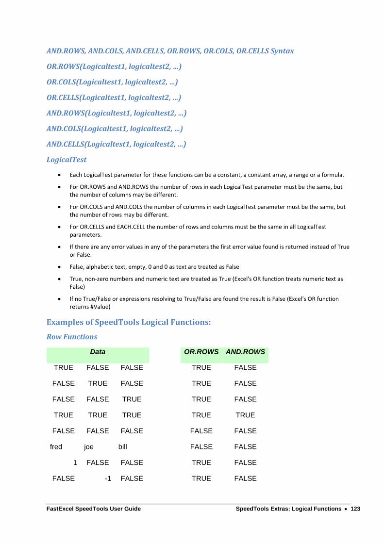
FastExcel SpeedTools User Guide SpeedTools Extras: Logical Functions 123
AND.ROWS,AND.COLS,AND.CELLS,OR.ROWS,OR.COLS,OR.CELLSSyntax
OR.ROWS(Logicaltest1,logicaltest2,…)
OR.COLS(Logicaltest1,logicaltest2,…)
OR.CELLS(Logicaltest1,logicaltest2,…)
AND.ROWS(Logicaltest1,logicaltest2,…)
AND.COLS(Logicaltest1,logicaltest2,…)
AND.CELLS(Logicaltest1,logicaltest2,…)
LogicalTest
Each LogicalTest parameter for these functions can be a constant, a constant array, a range or a formula.
For OR.ROWS and AND.ROWS the number of rows in each LogicalTest parameter must be the same, but the number of columns may be different.
For OR.COLS and AND.COLS the number of columns in each LogicalTest parameter must be the same, but the number of rows may be different.
For OR.CELLS and EACH.CELL the number of rows and columns must be the same in all LogicalTest parameters.
If there are any error values in any of the parameters the first error value found is returned instead of True or False.
False, alphabetic text, empty, 0 and 0 as text are treated as False
True, non‐zero numbers and numeric text are treated as True (Excel's OR function treats numeric text as False)
If no True/False or expressions resolving to True/False are found the result is False (Excel's OR function returns #Value)
ExamplesofSpeedToolsLogicalFunctions:
RowFunctions
Data OR.ROWS AND.ROWS
TRUE FALSE FALSE TRUE FALSE
FALSE TRUE FALSE TRUE FALSE
FALSE FALSE TRUE TRUE FALSE
TRUE TRUE TRUE TRUE TRUE
FALSE FALSE FALSE FALSE FALSE
fred joe bill FALSE FALSE
1 FALSE FALSE TRUE FALSE
FALSE -1 FALSE TRUE FALSE

FastExcel SpeedTools User Guide SpeedTools Extras: Logical Functions 124
FALSE FALSE 0.001 TRUE FALSE
TRUE TRUE TRUE TRUE TRUE
TRUE joe bill TRUE FALSE
fred TRUE bill TRUE FALSE
fred joe TRUE TRUE FALSE
FALSE joe bill FALSE FALSE
fred FALSE bill FALSE FALSE
fred joe FALSE FALSE FALSE
FALSE TRUE FALSE TRUE FALSE
TRUE 0 FALSE TRUE FALSE
FALSE FALSE
FALSE FALSE
The OR.ROWS formula is array‐entered (Control‐Shift‐Enter) in the column as
{=OR.ROWS(A2:A21,B2:B21,C2:C21)}
The AND.ROWS formula is array‐entered (Control‐Shift‐Enter) in the column as
{=AND.ROWS(A2:A21,B2:B21,C2:C21)}
The functions have evaluated each row of the data to produce a corresponding True/False
ColumnFunctions:
Data
TRUE FALSE FALSE
1 TRUE FALSE
-1 FALSE 0
1 TRUE 0
{=AND.COLS(A55:C58)}
TRUE FALSE FALSE
{=OR.COLS(A55:C58)}
TRUE TRUE FALSE

FastExcel SpeedTools User Guide SpeedTools Extras: Logical Functions 125
The functions have evaluated each column of the data to produce a corresponding True/False
CELLFunctions:
Data More Data OR.CELLS AND.CELLS
TRUE FALSE FALSE FALSE FALSE TRUE TRUE FALSE TRUE FALSE FALSE FALSE
FALSE TRUE FALSE FALSE FALSE TRUE FALSE TRUE TRUE FALSE FALSE FALSE
FALSE FALSE TRUE TRUE FALSE TRUE TRUE FALSE TRUE FALSE FALSE TRUE
TRUE TRUE TRUE TRUE TRUE FALSE TRUE TRUE TRUE TRUE TRUE FALSE
FALSE FALSE FALSE TRUE FALSE FALSE TRUE FALSE FALSE FALSE FALSE FALSE
fred joe bill TRUE TRUE TRUE TRUE TRUE TRUE FALSE FALSE FALSE
1 FALSE FALSE FALSE FALSE FALSE TRUE FALSE FALSE FALSE FALSE FALSE
FALSE -1 FALSE TRUE FALSE TRUE TRUE TRUE TRUE FALSE FALSE FALSE
FALSE FALSE 0.001 TRUE TRUE FALSE TRUE TRUE TRUE FALSE FALSE FALSE
TRUE TRUE TRUE FALSE TRUE FALSE TRUE TRUE TRUE FALSE TRUE FALSE
TRUE joe bill fred TRUE FALSE TRUE TRUE FALSE FALSE FALSE FALSE
fred TRUE bill FALSE FALSE TRUE FALSE TRUE TRUE FALSE FALSE FALSE
fred joe TRUE FALSE TRUE TRUE FALSE TRUE TRUE FALSE FALSE TRUE
FALSE joe bill FALSE FALSE FALSE FALSE FALSE FALSE FALSE FALSE FALSE
fred FALSE bill FALSE FALSE TRUE FALSE FALSE TRUE FALSE FALSE FALSE
fred joe FALSE TRUE FALSE FALSE TRUE FALSE FALSE FALSE FALSE FALSE
FALSE TRUE FALSE TRUE TRUE TRUE TRUE TRUE TRUE FALSE TRUE FALSE
TRUE 0 FALSE FALSE FALSE FALSE TRUE FALSE FALSE FALSE FALSE FALSE
FALSE FALSE FALSE FALSE FALSE FALSE
FALSE FALSE FALSE FALSE FALSE FALSE
{=OR.CELLS($A$2:$C$21,$E$2:$G$19)}
{=AND.CELLS($A$2:$C$21,$E$2:$G$19)}
The functions have evaluated each corresponding element in the 2 data tables to produce a corresponding array of True/False.
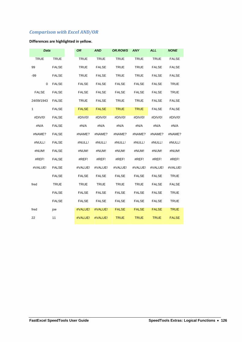
FastExcel SpeedTools User Guide SpeedTools Extras: Logical Functions 126
ComparisonwithExcelAND/OR
Differences are highlighted in yellow.
Data OR AND OR.ROWS ANY ALL NONE
TRUE TRUE TRUE TRUE TRUE TRUE TRUE FALSE
99 FALSE TRUE FALSE TRUE TRUE FALSE FALSE
-99 FALSE TRUE FALSE TRUE TRUE FALSE FALSE
0 FALSE FALSE FALSE FALSE FALSE FALSE TRUE
FALSE FALSE FALSE FALSE FALSE FALSE FALSE TRUE
24/09/1943 FALSE TRUE FALSE TRUE TRUE FALSE FALSE
1 FALSE FALSE FALSE TRUE TRUE FALSE FALSE
#DIV/0! FALSE #DIV/0! #DIV/0! #DIV/0! #DIV/0! #DIV/0! #DIV/0!
#N/A FALSE #N/A #N/A #N/A #N/A #N/A #N/A
#NAME? FALSE #NAME? #NAME? #NAME? #NAME? #NAME? #NAME?
#NULL! FALSE #NULL! #NULL! #NULL! #NULL! #NULL! #NULL!
#NUM! FALSE #NUM! #NUM! #NUM! #NUM! #NUM! #NUM!
#REF! FALSE #REF! #REF! #REF! #REF! #REF! #REF!
#VALUE! FALSE #VALUE! #VALUE! #VALUE! #VALUE! #VALUE! #VALUE!
FALSE FALSE FALSE FALSE FALSE FALSE TRUE
fred TRUE TRUE TRUE TRUE TRUE FALSE FALSE
FALSE FALSE FALSE FALSE FALSE FALSE TRUE
FALSE FALSE FALSE FALSE FALSE FALSE TRUE
fred joe #VALUE! #VALUE! FALSE FALSE FALSE TRUE
22 11 #VALUE! #VALUE! TRUE TRUE TRUE FALSE

FastExcel SpeedTools User Guide SpeedTools Extras: Logical Functions 127
IFERRORXFunction
Use this function for trapping and handling errors in formulas. It is similar to the IFERROR function available in Excel
2007 and later Excel versions, but also works with earlier Excel versions and has options to pass through #N/A and
#Value.
Description
Returns a value you choose if the formula expression returns an error, otherwise returns the result of the formula
expression.
Sometimes you need to be able to trap all error values except #N/A or #VALUE so that the error value is allowed to
propagate through dependent formulas. So IFERRORX allows you to optionally request that #N/A and/or #Value
are NOT considered as errors by IFERRORX but are passed through instead.
Its more efficient to use IFERRORX instead of formulas like =IF(ISERROR(VLOOKUP(A1,B1:C65000,2,FALSE)),”Not
Found”, VLOOKUP(A1,B1:C65000,2,FALSE))
IFERRORX is a multi‐threaded, non‐volatile array function.
IFERRORXSyntax
IFERRORX(TheExpression,Value_if_error,Exclude_NA,Exclude_Value)
TheExpression–Required
The value of formula expression to be checked for an error.
Value_if_error–Required
The value to return if Expression evaluates to an error.
Exclude_NA–Optional
If TRUE and the error is #N/A do NOT evaluate as an error and so return #N/A. Default FALSE.
Exclude_Value–Optional
If TRUE and the error is #VALUE do NOT evaluate as an error and so return #VALUE. Default FALSE.
Remarks
If the IFERRORX function is contained in an array formula and TheExpression returns an array of values then
IFERRORX handles each value in the array individually.
If TheExpression evaluates to an empty cell IFERRORX treats it as a zero. This behaviour is not the same as the
IFERROR function in Excel 2007 and later which treats an empty cell as an empty string.
The IFERRORX function is thread‐safe.
Examples
=IFERRORX(VLOOKUP(A1,B1:C65000,2,FALSE),”Not Found”) instead of
=IF(ISERROR(VLOOKUP(A1,B1:C65000,2,FALSE)),”Not Found”, VLOOKUP(A1,B1:C65000,2,FALSE))
=IFERRORX(200/5,”Division Error”) returns 40

FastExcel SpeedTools User Guide SpeedTools Extras: Logical Functions 128
=IFERRORX(200/0,”Division Error”) returns “Division error”
=IFERRORX(MATCH(99,{1,2,3,4,5,6,7,8,99,100},0),0) returns 9 (the 9th position)
=IFERRORX(MATCH(99,{1,2,3,4,5,6,7,8,9},0),0) returns 0 (99 is not found so the #N/A is replaced by Value_if_error)
=IFERRORX(MATCH(99,{1,2,3,4,5,6,7,8,9},0),0,TRUE) returns #N/A (Exclude_NA is TRUE so the #N/A is not
considered an error)

FastExcel SpeedTools User Guide SpeedTools Extras: Reference Functions 129
SpeedToolsExtras:ReferenceFunctions EVAL ‐ Evaluates strings as formulas.
PREVIOUS ‐ Returns the value of the cell at the previous calculation.
SETMEM ‐ Store the result of an expression to be retrieved later in the same formula
GETMEM ‐ Retrieve a result that was stored by SETMEM

FastExcel SpeedTools User Guide SpeedTools Extras: Reference Functions 130
EVALfunction:evaluateastring
The EVAL is an array function that evaluates a string as though it was an Excel formula or an Excel defined name,
and returns the result of the evaluation, or #N/A if the string cannot be evaluated.
EVAL is NOT multi‐threaded, is volatile and an array function.
EVALSyntax
EVAL(theInput)
theInput
any mixture of constants, functions, expressions, names and ranges that evaluates to a string. If the resulting string
cannot be evaluated as an excel formula or defined name the function will return #Value.
EVALRemarksandLimits
EVALisavolatilefunction.
Because EVAL is a volatile function every formula containing an EVAL function will be recalculated at every
recalculation.
Unqualifiedcellreferences
The input string is evaluated as though it was on the worksheet in which the function has been entered. This means
that unqualified cell references like F7 will be evaluated as referring to F7 on this sheet, regardless of which sheet is
active. To refer to cells on other sheets use qualified references like Sheet3!F7.
ArrayFormulae
The input string is always evaluated as though it had been array‐entered. An array of multiple results is returned
where appropriate.
DateLiterals
EVAL always interprets date literals as US style dates (MMDDYY).
Maximum255characters
EVAL will evaluate a maximum of 255 characters

FastExcel SpeedTools User Guide SpeedTools Extras: Reference Functions 131
PREVIOUSFunction
PREVIOUS returns the value of the cell at the previous calculation.
PREVIOUS allows you to get the value from the previous calculation for the cell containing the PREVIOUS function.
Normally if you create a formula that refers to the cell that contains the formula, Excel detects a circular reference
that requires using iteration to solve.
PREVIOUS does NOT cause a circular calculation.
You can use PREVIOUS as a parameter of a VBA UDF. This is useful when you have a slow UDF that you want to be
able to short‐circuit under certain conditions. For example if your UDF retrieves data from a remote server you may
only want to retrieve a new value when the server has been refreshed.
PREVIOUS is NOT thread‐safe, is optionally volatile and does not handle arrays.
PreviousSyntax
PREVIOUS(Volatile)
Volatile
Optional (default True). True causes the function to be calculated at every recalculation.
Do not use False for this argument when the formula containing the function uses or refers to a cell containing a
volatile function.
RemarksandLimits
PREVIOUS is NOT a thread‐safe function, and so any formula containing PREVIOUS will not take advantage of
Excel’s multi‐threaded calculation.
Do not use False for the Volatile argument when the formula containing the function uses or refers to a cell
containing a volatile function.
When a formula containing PREVIOUS is entered, the value from the previous recalculation will be reset.
Examples
=MyUDF(Refresh,theInput,PREVIOUS(FALSE))
If MyUDF is a VBA function that retrieves data from a remote server based on the parameters in theInput, you
could program it to only get the data from the remote server when the Refresh switch was true, otherwise it could
return the value from the last calculation.
=IF(A1>PREVIOUS(),A1,PREVIOUS())
Gives the largest value that cell A1 has ever contained.
=PREVIOUS(FALSE)+A1
Gives a cumulative sum of all the numbers that have changed in A1.
Note that if the same number is entered twice in succession in cell A1 this formula will NOT accumulate the same
number twice.

FastExcel SpeedTools User Guide SpeedTools Extras: Reference Functions 132
=IF(COUNTA(C1)>0,PREVIOUS(FALSE)+1,0)
Counts the number of times the contents of cell C1 has been changed, reset to zero if C1 is cleared or the contents
deleted.
Note that if the same value is entered twice in succession in cell A1 this formula will NOT increment the change
count.
FastExcel SpeedTools User Guide SpeedTools Extras: Reference Functions 133
SETMEMandGETMEMFunctions
Optimise your formulas by storing and retrieving the results of very calculation‐intensive expressions used more
than once in a formula.
Description
The SETMEM and GETMEM functions are thread‐safe functions that you can use to avoid repeated calculation of
expressions that occur more than once in the same formula.
Use SETMEM to store in memory the results of calculating a calculation‐intensive formula expression so that you
can replace the later repeats of the formula expression with GETMEM.
This can save time when the additional cost of using SETMEM and GETMEM is less than the cost of the repeated
calculation of the calculation‐intensive formula expression.
You can use GETMEM as many times as you like within a formula to retrieve the previously stored results.
SETMEM and GETMEM are both thread‐safe, non‐volatile, array functions
SETMEMSyntax
SETMEM(TheValue,SetID)
TheValue
The value, range, array, or expression result to be stored.
SetID(Optional.Default“A”)
The ID (string) for the stored values. Default is “A”.
GETMEMSyntax
GETMEM(SetID)
SetID(Optional.Default“A”)
The ID (string) for the previously stored temporary valus. Default is “A”.

FastExcel SpeedTools User Guide SpeedTools Extras: Array-Handling Functions 134
SpeedToolsExtras:Array‐HandlingFunctionsThese array‐handling functions allow you to solve some problems with the use of multiple ranges and/or
array formulas.
COL.ARRAY ‐ Appends Ranges/Arrays column‐wise
ROW.ARRAY ‐ Appends Ranges/Arrays row‐wise
REVERSE.ARRAY ‐ Reverse the rows, columns or both in an array.
PAD.ARRAY ‐ Resize and/or pad an array
VECTOR ‐ Outputs a sequence of numbers as a column or row vector.

FastExcel SpeedTools User Guide SpeedTools Extras: Array-Handling Functions 135
COL.ARRAYFunction
Creates a single array from multiple arrays or ranges by appending up to 28 Range /Array arguments alongside one another column wise. Missing cells in the output array can be filled with Pad characters, for example 0 or "".
COL.ARRAY is a multi-threaded, non-volatile array function.
COL.ARRAYSyntax
COL.ARRAY(Pad,Arg1,Arg2,…,Arg28)
Pad(Optional,default#N/A)
A cell or character or digit to be used to fill unused cells in the output array, for example 0 or “”.
When the Arrays or ranges to be appended do not have equally sized dimensions the gaps will be filled
with the Pad character. Use zero if you want to append differently‐sized numeric arrays and pass the
output to an aggregating function such as SUM() or a single‐cell array formula.
Arg1toArg28
Ranges or arrays to be appended. Each Range/Array is placed in the output array starting in row 1 of the
next available output column.
The ranges to be appended can be on different sheets.
COL.ARRAYExamples
A2:C2 contains 1,2,3
B4:D4 contains 4,5,6
{=COL.ARRAY(A2:C2,B4:D4)} array entered into C20:H20 returns
(A2:C2 cannot be a PAD character so is treated as Arg1)
{=COL.ARRAY(0,A2:C2,{100;200;300},B4:D4)} array entered into C7:J10 returns
The row dimension of the output array is the maximum number of rows in any of the arguments. The
column dimension of the output array is the sum of the number of columns in each argument. So the
output array is 3 rows deep by 7 columns.
The values from each argument are placed in turn into the output array, appending column‐wise to the
right.

FastExcel SpeedTools User Guide SpeedTools Extras: Array-Handling Functions 136
For the arguments that have less than 3 rows the missing rows are filled with the pad character (zero in
this case). Because the formula was array‐entered into 4 rows by 8 columns Excel has added #N/A in the
4th row and 8th column.
Entering =SUM(COL.ARRAY(0,A2:C2,{100;200;300},B4:D4)) (NOT as an array formula) returns 621, which
is the sum of the values in the output array.
Entering =AVERAGE(COL.ARRAY(0,A2:C2,{100;200;300},B4:D4)) (NOT an array formula) returns 29.57
which is 621 divided by the number of cells in the output array (21).
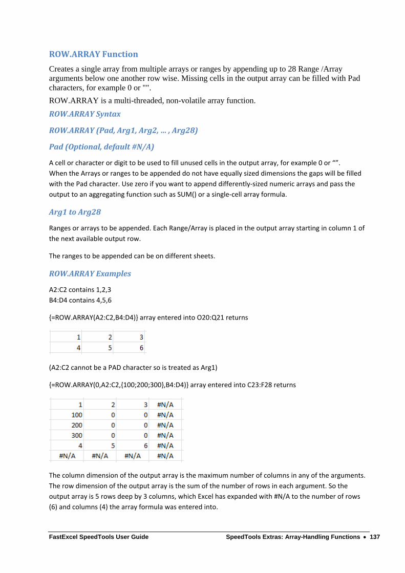
FastExcel SpeedTools User Guide SpeedTools Extras: Array-Handling Functions 137
ROW.ARRAYFunction
Creates a single array from multiple arrays or ranges by appending up to 28 Range /Array arguments below one another row wise. Missing cells in the output array can be filled with Pad characters, for example 0 or "".
ROW.ARRAY is a multi-threaded, non-volatile array function.
ROW.ARRAYSyntax
ROW.ARRAY(Pad,Arg1,Arg2,…,Arg28)
Pad(Optional,default#N/A)
A cell or character or digit to be used to fill unused cells in the output array, for example 0 or “”.
When the Arrays or ranges to be appended do not have equally sized dimensions the gaps will be filled
with the Pad character. Use zero if you want to append differently‐sized numeric arrays and pass the
output to an aggregating function such as SUM() or a single‐cell array formula.
Arg1toArg28
Ranges or arrays to be appended. Each Range/Array is placed in the output array starting in column 1 of
the next available output row.
The ranges to be appended can be on different sheets.
ROW.ARRAYExamples
A2:C2 contains 1,2,3
B4:D4 contains 4,5,6
{=ROW.ARRAY(A2:C2,B4:D4)} array entered into O20:Q21 returns
(A2:C2 cannot be a PAD character so is treated as Arg1)
{=ROW.ARRAY(0,A2:C2,{100;200;300},B4:D4)} array entered into C23:F28 returns
The column dimension of the output array is the maximum number of columns in any of the arguments.
The row dimension of the output array is the sum of the number of rows in each argument. So the
output array is 5 rows deep by 3 columns, which Excel has expanded with #N/A to the number of rows
(6) and columns (4) the array formula was entered into.

FastExcel SpeedTools User Guide SpeedTools Extras: Array-Handling Functions 138
The values from each argument are placed in turn into the output array, appending row‐wise to the
bottom.
For the arguments that have less than 3 columns the missing rows are filled with the pad character (zero
in this case). Because the formula was array‐entered into 6 rows by 4 columns Excel has added #N/A in
the 6th row and 4th column.
Entering =SUM(ROW.ARRAY(0,A2:C2,{100;200;300},B4:D4)) (NOT as an array formula) returns 621,
which is the sum of the values in the output array.
Entering =AVERAGE(ROW.ARRAY(0,A2:C2,{100;200;300},B4:D4)) (NOT an array formula) returns 41.4
which is 615 divided by the number of cells in the output array (15).
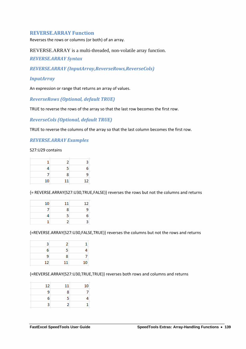
FastExcel SpeedTools User Guide SpeedTools Extras: Array-Handling Functions 139
REVERSE.ARRAYFunctionReverses the rows or columns (or both) of an array.
REVERSE.ARRAY is a multi-threaded, non-volatile array function.
REVERSE.ARRAYSyntax
REVERSE.ARRAY(InputArray,ReverseRows,ReverseCols)
InputArray
An expression or range that returns an array of values.
ReverseRows(Optional,defaultTRUE)
TRUE to reverse the rows of the array so that the last row becomes the first row.
ReverseCols(Optional,defaultTRUE)
TRUE to reverse the columns of the array so that the last column becomes the first row.
REVERSE.ARRAYExamples
S27:U29 contains
{= REVERSE.ARRAY(S27:U30,TRUE,FALSE)} reverses the rows but not the columns and returns
{=REVERSE.ARRAY(S27:U30,FALSE,TRUE)} reverses the columns but not the rows and returns
{=REVERSE.ARRAY(S27:U30,TRUE,TRUE)} reverses both rows and columns and returns

FastExcel SpeedTools User Guide SpeedTools Extras: Array-Handling Functions 140
By comparison {=TRANSPOSE(S27:U30)} returns

FastExcel SpeedTools User Guide SpeedTools Extras: Array-Handling Functions 141
PAD.ARRAYFunctionPAD.ARRAY allows you to resize (expand or contract) an array and to control the PAD value to be used
for the expanded cells. The expanded cells are the cells in the output array that are not present in the
input array.
PAD.ARRAY is a multi-threaded, non-volatile array function.
PAD.ARRAYSyntax
PAD.ARRAY(Pad,InputArray,NumRows,NumCols)
Pad(Optional,defaultzero)
The value to use for the expanded cells. The default value is zero.
InputArray(required)
An array expression, formula or range that returns an array of values.
NumRows(Optional,default‐1)
The number of rows in the output array can be larger or smaller than the input array.
If NumRows is ‐1 (default) and PAD.ARRAY is entered into a multi‐cell array formula then the number of
rows in the multi‐cell array formula will be used.
If NumRows is ‐1 (default) and PAD.ARRAY is part of a single‐cell formula then the number of rows in the
InputArray will be used.
If NumRows is a positive integer it will control the number of rows in the output array.
NumColumns(Optional,default‐1)
The number of columns in the output array can be larger or smaller than the input array.
If NumColumns is ‐1 (default) and PAD.ARRAY is entered into a multi‐cell array formula then the number
of columns in the multi‐cell array formula will be used.
If NumColumns is ‐1 (default) and PAD.ARRAY is part of a single‐cell formula then the number of columns
in the InputArray will be used.
If NumColumns is a positive integer it will control the number of columns in the output array.

FastExcel SpeedTools User Guide SpeedTools Extras: Array-Handling Functions 142
VECTORFunctionVECTOR returns a column or row of increasing or decreasing positive or negative integers
VECTOR is a multi-threaded, non-volatile array function.
VECTORSyntax
VECTOR(StartValue,EndValue,Step,Row)
StartValue(Optional,default1)
The first number. Can be positive or negative. If omitted the value 1 will be used
EndValue(Required)
The last number: can be positive or negative.
Step(Optional,default1)
The increment between numbers. Can be positive or negative. If omitted the value 1 or ‐1 will be used.
If the sign of step is not a valid increment for StartValue and EndValue its sign will be reversed.
Row(Optional,defaultTRUE)
If ROW is TRUE then a row of numbers will be generated. If FALSE a Column of numbers will be
generated.
VECTORExamples
{=VECTOR(,6)} returns a row containing 1 to 6
(=VECTOR(1,6,1,FALSE)} returns a column containing 1 to 6
{=VECTOR(6,1,‐1,FALSE)} returns a column containing 6 to 1
{=VECTOR(‐6,‐1,‐1,FALSE)} returns a column containing ‐6 to ‐1
{=VECTOR(‐3,2,‐1,FALSE)} returns a column containing ‐3 to +2
{=VECTOR(‐3,6,‐2,FALSE)} returns a column containing ‐3,‐1,1,3,5

FastExcel SpeedTools User Guide SpeedTools Extras: Information Functions 143
SpeedToolsExtras:InformationFunctionsAdditional information functions:
ISLIKE ‐ wildcard pattern testing for text strings
Rgx.ISLIKE ‐ regular expression pattern testing for text strings
HASFORMULA ‐ returns true if the cell contains a formula
COUNTROWS and COUNTCOLS count the number of rows or columns from a referenced cell to the last visible non‐empty cell in the row or column.
COUNTCONTIGROWS and COUNTCONTIGCOLS count the number of rows or columns from a referenced cell to before the next visible empty cell.
COUNTUSEDROWS and COUNTUSEDCOLS count the number of rows or columns from a referenced cell to the last cell in the used range.
CALCSEQCOUNTREF, CALCSEQCOUNTSET, CALCSEQCOUNTVOL simplify the tracing of Excel’s
calculation sequence and determining if a function is volatile.

FastExcel SpeedTools User Guide SpeedTools Extras: Information Functions 144
ISLIKEarrayfunctionforpattern‐matchingstrings
The ISLIKE function performs a wild‐card comparison between a string and a pattern using VBA Like, and returns
True if the string matches the pattern, or False if it does not or an error occurs.
ISLIKE can be used as an array function
ISLIKE is multithreaded, is non‐volatile and is an array function.
ISLIKESyntax
ISLIKE(theString,thePattern,CaseSensitive)
theString
An expression, constant or Range that can be resolved to a string or array of strings: the string(s) to be compared to
the pattern. If theString contains numeric values they will be converted to strings.
ThePattern
An expression, constant or Range that can be resolved to a string or arrays of strings: the pattern(s) to be used in
the comparison.
Patterns can contain:
* Any number of characters, including none
? Any single character
ISLIKEArrayfunctionusage
When ISLIKE is used as an array function or inside an array formula each of the input arguments can be a single
value, a one or two‐dimensional array or a one or two‐dimensional range.
If the dimensions of the two input arguments do not match, the smaller dimension will be wrapped: for example
=ISLIKE(“Fred7”,{”*3”,”*5”,”*7”}) compares Fred7 to each of *3, *5, *7 in turn and returns {False,False,True}
ISLIKEExamples
True =ISLIKE( "aBBBa" ,"a*a")
True =ISLIKE("BAT123khg","B?T*")
False =ISLIKE("CAT123khg","B?T*")

FastExcel SpeedTools User Guide SpeedTools Extras: Information Functions 145
Rgx.ISLIKEfunction
Tests whether a string matches a Regular Expression Pattern.
Rgx.ISLIKE is a multi‐threaded, non‐volatile array function.
Rgx.ISLIKESyntax
Rgx.ISLIKE(String,RegExp,Case_Sensitive)
The first 2 parameters are required; the last parameter is optional.
String(required)
Text to be matched by the Regular Expression Pattern.
RegExp(required)
Specifies the Regular Expression to be used when matching the String.
Case_Sensitive(optional)
TRUE to make the pattern‐matching case‐sensitive. The default is FALSE.
Rgx.ISLIKEExample
The Numbers are in A36:A42, stored as text.
The RegEx Pattern is in C34.
The Rgx.ISLIKE formula is copied down in each cell of C36:C42.
You can also use Rgx.ISLIKE as an array formula
{=Rgx.ISLIKE(A36:A42,C34)} would give the same results as the 7 individual formulas.

FastExcel SpeedTools User Guide SpeedTools Extras: Information Functions 146
HASFORMULAfunction
The HASFORMULA function returns true if any of the cells in the range contain a formula.
HASFORMULA is NOT multi‐threaded, NOT volatile and is NOT an array function.
HASFORMULASyntax
HASFORMULA(theRange)
theRange
Any valid range reference.
The function returns true if any of the cells in the range contains a formula, otherwise false.
HASFORMULARemarks
The function considers the following as formulae:
=2
+2
=a1
=”Text”
=NOW()
=RangeName
The function will return False for the following:
2
45
“Text”

FastExcel SpeedTools User Guide SpeedTools Extras: Information Functions 147
CalculationSequenceandCountingfunctions
SpeedTools contains three functions to help trace Excel’s calculation sequence.
Two of these functions increment a counter, and the third allows you to reset the counter.
CALCSEQCOUNTREFFunction
CalcSeqCountRef returns the value of the calculations counter, and is dependent on a cell reference, so you can use
it to count the number of time a cell is calculated.
CalcSeqcountRefSyntax
CalcSeqCountRef(theRange)
theRange
A reference to an excel cell. At each recalculation Excel will calculate CalcSeqCountRef if the cell referred to by
theRange has changed or been recalculated.
CalcSeqCountRefRemarks
The function uses a single global calculation counter, so a workbook containing multiple formulae containing
CalcSeqCountRef will show the sequence in which they were calculated.
Entering CalcSeqCountRef into a cell using the Function Wizard/Palette will increment the calculation counter
several times because the Function Wizard attempts to show you the result of the function at each step.
To reset the calculations counter either run the ZeroCalcSeq macro from ToolsMacros, or use the
CalcSeqCountSet function.
See also the CalcSeqCountVol function, which is a volatile function which increments the same calculations
counter.
CALCSEQCOUNTSETFunction
This function allows you to set the calculation counter used by CalcSeqCountRef and CalcSeqCountVol to a value.
CalcSeqCountSetSyntax
CalcSeqCountSet(theInput)
TheInput
an integer value or a reference that can be resolved to an integer value.
This value is used to reset the calculation counter each time the function is executed. Alternatively you can run the
ZeroCalcSeq macro from ToolsOptions, which will set the counter to zero.
CALCSEQCOUNTVOLfunction
This function is a volatile version of CalcSeqCountRef.
CalcSeqCountVolSyntax
CalcSeqCountVol()

FastExcel SpeedTools User Guide SpeedTools Extras: Information Functions 148
The function has no arguments and is volatile. The function will increment the calculation counter at each
calculation or recalculation.

FastExcel SpeedTools User Guide SpeedTools Extras: Information Functions 149
FunctionsforcountingRowsandColumns
These functions give you the ability to find the number of rows or columns to the last empty cell, the next empty
cell, or the last cell in the used range:
COUNTROWS and COUNTCOLS count the number of rows or columns from a referenced cell to the last visible non‐empty cell in the row or column.
COUNTCONTIGROWS and COUNTCONTIGCOLS count the number of rows or columns from a referenced cell to before the next visible empty cell.
COUNTUSEDROWS and COUNTUSEDCOLS count the number of rows or columns from a referenced cell to the last cell in the used range.
You can use these functions in Dynamic Range names and for the number of rows and columns arguments in
OFFSET.
COUNTROWS and COUNTCONTIGROWS can count rows in either a single column or multiple adjacent columns.
Similarly COUNTCOLS and COUNTCONTIGCOLS can count columns in either a single row or multiple adjacent rows.
All these functions (COUNTROWS, COUNTCOLS, COUNTCONTIGROWS, COUNTCONTIGCOLS, COUNTUSEDROWS
and COUNTUSEDCOLS) are volatile functions.
Changing cell visibility using Automatic or Advanced filter will trigger a recalculation of COUNTROWS,
COUNTCOLS, COUNTCONTIGROWS and COUNTCONTIGCOLS.
Changing cell visibility using Hide, Unhide or by setting width or height to zero will NOT trigger a recalculation of
COUNTROWS, COUNTCOLS, COUNTCONTIGROWS and COUNTCONTIGCOLS.
These functions are volatile, NOT thread‐safe, NOT array‐capable functions.

FastExcel SpeedTools User Guide SpeedTools Extras: Information Functions 150
COUNTROWSFunction
The COUNTROWS function counts the number of rows from a reference row to the last visible non‐empty cell in
the referenced columns.
COUNTROWSSyntax
COUNTROWS(theColumns)
TheColumns
A range reference to a cell or cells in the columns whose rows are to be counted.
COUNTROWS counts the number of rows, including blanks and empty cells down to the last visible non‐empty cell.
The count includes the top row of the referenced cell.
If theColumns refers to more than one adjacent column then the count gives the largest row count found for the
columns.
COUNTROWSRemarks
COUNTROWS is a volatile function.
If the reference specified for theColumns contains more than one row, the top row will be used.
If the reference specified for theColumns contains more than one column, the last visible non‐empty row in each
column will be found, and the largest row count will be returned.
COUNTROWS uses the same criteria as Ctrl‐Up Arrow to detect empty cells. The last row found is equivalent to
selecting row 65536 and pressing Ctrl‐Up‐Arrow, except that it will stop at the cell specified by theColumns.
COUNTROWS will return 1 if the cell specified by theColumns is empty and there are no other visible non‐empty
cells below theColumns
A cell that contains nothing but is formatted is treated as an empty cell.
A cell that contains ‘ will look empty but will be treated as a non‐empty cell.
Invisible cells can be created using Automatic or Advanced Filter, hiding rows or columns, or setting row heights or
column widths to zero.
If the last row(s) in the range are not visible then COUNTROWS will not count them.
If intermediate row(s) in the range are not visible COUNTROWS will count them.
Countrows should be used
with care on ranges with
hidden rows or rows with
zero heights.
Because hiding rows/columns or setting width/heights to zero does not
trigger a recalculation COUNTROWS may show an incorrect value even
in automatic mode until the workbook is recalculated. Changing the
Automatic or Advanced filter does trigger a recalculation.
COUNTROWSExample
Assuming that cell B55 contains 10 and there are no other non‐empty cells in column B then:
=COUNTROWS(B4) returns 52 (51 rows from B4 to B55 plus row 4 itself).
FastExcel SpeedTools User Guide SpeedTools Extras: Information Functions 151
COUNTCONTIGROWSFunction
The COUNTCONTIGROWS function counts the number of rows from a reference row down to the last cell before
the next visible empty cell in the referenced columns.
COUNTCONTIGROWSSyntax
COUNTCONTIGROWS(theColumns)
TheColumns
A range reference to a cell or cells in the columns whose rows are to be counted.
COUNTCONTIGROWS counts the number of rows downwards from the referenced cell to the cell before the first
visible empty cell found.
The count includes the top row of the referenced cell.
If theColumns refers to more than one adjacent column then the count gives the largest row count found for the
columns.
COUNTCONTIGROWSRemarks
COUNTCONTIGROWS is a volatile function.
If the reference specified for theColumns contains more than one row, the top row will be used.
If the reference specified for theColumns contains more than one column, the last non‐empty row before the first
empty cell in each column will be found, and the largest rowcount will be returned.
COUNTCONTIGROWS uses the same criteria as Ctrl‐Down Arrow to detect empty cells, except when the reference
cell or the cell below the reference cell is empty.
COUNTCONTIGROWS will return 1 if the cell specified by theColumns is empty and the next cell down is also
empty.
If the cell specified by theColumns is empty but the cells below it are not empty then COUNTCONTIGROWS will
look downwards from the cell below the cell specified by theColumns.
A cell that contains nothing but is formatted is treated as an empty cell.
A cell that contains ‘ will look empty but will be treated as a non‐empty cell.
Invisible cells can be created using Automatic or Advanced Filter, hiding rows or columns, or setting row heights or
column widths to zero.
If intermediate empty row(s) in the range are not visible COUNTCONTIGROWS will NOT treat them as empty.
Countcontigrows is not
recommended for ranges
with hidden rows or rows
with zero heights.
Because hiding rows/columns or setting width/heights to zero does not
trigger a recalculation COUNTCONTIGROWS may show an incorrect
value even in automatic mode until the workbook is recalculated.
Changing the Automatic or Advanced filter does trigger a recalculation.
COUNTCONTIGROWS is not recommended for ranges containing
hidden rows or rows with zero heights.

FastExcel SpeedTools User Guide SpeedTools Extras: Information Functions 152
COUNTCONTIGROWSExample
Assuming that cells B4:B55 contain 10 and cell B2:B3 and cell B56 are empty then:
=COUNTCONTIGROWS(B4) returns 52 (51 consecutive non‐empty rows from B5 to B55 plus row 4 itself).
=COUNTCONTIGROWS(B2) returns 1 (the cell below B2 is empty)
=COUNTCONTIGROWS(B3) returns 53 (52 consecutive non‐empty rows from B4 to B55 plus row 3 itself even
though B3 is empty).

FastExcel SpeedTools User Guide SpeedTools Extras: Information Functions 153
COUNTUSEDROWSFunction
The COUNTUSEDROWS function counts the number of rows down to the end of the used range for this sheet.
COUNTUSEDROWSSyntax
COUNTUSEDROWS(theRow)
TheRow
A range reference to a row.
COUNTUSEDROWS counts the number of rows, including blanks and empty cells down to the end of the used range
for the sheet containing theRow.
The count includes the top row of the referenced range.
COUNTUSEDROWSRemarks
COUNTUSEDROWS is a volatile function.
If the reference specified for theRow contains more than one row, the top row will be used.
The used range may contain empty rows or columns.
Whenever the COUNTUSEDROWS function is calculated the used range for the worksheet containing theRow will
be reset.
COUNTUSEDROWSExample
Assuming that cell B55 contains 10 and cell Z75 is empty but coloured yellow , and no other cells have been
formatted then:
=COUNTUSEDROWS(B4) returns 72 (row 75 is the last row in the used range less rows 1‐3).
FastExcel SpeedTools User Guide SpeedTools Extras: Information Functions 154
COUNTCOLSFunction
The COUNTCOLS function counts the number of columns before the last visible non‐empty cell in the referenced
row.
COUNTCOLSSyntax
COUNTCOLS(theRows)
TheRows
A range reference to a cell or cells in the rows whose columns are to be counted.
COUNTCOLS counts the number of columns, including blanks and empty cells across to the right to the last visible
non‐empty cell.
The count includes the first column of the referenced cell.
If theRows refers to more than one adjacent row then the count gives the largest column count found for the rows.
COUNTCOLSRemarks
COUNTCOLS is a volatile function.
If the reference specified for theRows contains more than one column, the first column will be used.
If the reference specified for theRows contains more than one row, the last non‐empty column in each row will be
found, and the largest column count will be returned.
COUNTCOLS uses the same criteria as Ctrl‐Left Arrow to detect empty cells. The last column found is equivalent to
selecting column 256 and pressing Ctrl‐Left, except that it will stop at the cell specified by theRows.
COUNTCOLS will return 1 if the cell specified by theRows is empty and there are no other non‐empty cells to the
right of theRows
A cell that contains nothing but is formatted is treated as an empty cell.
A cell that contains ‘ will look empty but will be treated as a non‐empty cell.
Invisible cells can be created using Automatic or Advanced Filter, hiding rows or columns, or setting row heights or
column widths to zero.
If the last column(s) in the range are not visible COUNTCOLS will not count them.
If intermediate column(s) in the range are not visible COUNTCOLS will count them.
Countcols should be used
with care on ranges with
hidden rows or rows with
zero heights.
Because hiding rows/columns or setting width/heights to zero does not
trigger a recalculation COUNTCOLS may show an incorrect value even in
automatic mode until the workbook is recalculated. Changing the
Automatic or Advanced filter does trigger a recalculation.
COUNTCOLSExample
Assuming that cell D42 contains FRED and there are no other non‐empty cells in row 42 then:
=COUNTCOLS(B42) returns 3 (2 columns from B42 to D42 plus the B column itself).

FastExcel SpeedTools User Guide SpeedTools Extras: Information Functions 155
COUNTCONTIGCOLSFunction
The COUNTCONTIGCOLS function counts the number of COLUMNS from a reference row down to the last cell
before the next visible empty cell in the referenced columns.
COUNTCONTIGCOLSSyntax
COUNTCONTIGCOLS(theRows)
TheRows
A range reference to a cell or cells in the rows whose columns are to be counted.
COUNTCONTIGCOLS counts the number of columns across to the right from the referenced cell to the cell before
the first visible empty cell found.
The count includes the first column of the referenced cell.
If theRows refers to more than one adjacent row then the count gives the largest column count found for the rows.
COUNTCONTIGCOLSRemarks
COUNTCONTIGCOLS is a volatile function.
If the reference specified for theRows contains more than one column, the left‐most column will be used.
If the reference specified for theRows contains more than one row, the last non‐empty column before the first
empty cell in each row will be found, and the largest column count will be returned.
COUNTCONTIGCOLS uses the same criteria as Ctrl‐Right Arrow to detect empty cells, except when the reference
cell or the cell to the right of the reference cell is empty.
COUNTCONTIGCOLS will return 1 if the cell specified by theRows is empty and the next cell to the right is also
empty.
If the cell specified by theRows is empty but the cells to the right of it are not empty then COUNTCONTIGCOLS will
look to the right from the cell adjacent to the cell specified by theRows.
A cell that contains nothing but is formatted is treated as an empty cell.
A cell that contains ‘ will look empty but will be treated as a non‐empty cell.
Invisible cells can be created using Automatic or Advanced Filter, hiding rows or columns, or setting row heights or
column widths to zero.
If intermediate empty column(s) in the range are not visible COUNTCONTIGCOLS will NOT treat them as empty.
CountcontigCols is not
recommended for ranges
with hidden columns or
columns with zero heights.
Because hiding rows/columns or setting width/heights to zero does not
trigger a recalculation COUNTCONTIGCOLS may show an incorrect value
even in automatic mode until the workbook is recalculated. Changing
the Automatic or Advanced filter does trigger a recalculation.
COUNTCONTIGCOLS is not recommended for ranges containing hidden
columns or columns with zero heights.
COUNTCONTIGCOLSExample

FastExcel SpeedTools User Guide SpeedTools Extras: Information Functions 156
Assuming that cells C4:G4 contain 10 and cell A4, B4 and H4 are empty then:
=COUNTCONTIGCOLS(C4) returns 5 (4 consecutive non‐empty COLUMNS from D4 to G4 plus column C itself).
=COUNTCONTIGCOLS(A4) returns 1 (the cell to the right of A4 is empty)
=COUNTCONTIGCOLS(B4) returns 6 (5 consecutive non‐empty COLUMNS from C4 to G4 plus column B itself even
though B4 is empty).

FastExcel SpeedTools User Guide SpeedTools Extras: Information Functions 157
COUNTUSEDCOLSFunction
The COUNTUSEDCOLS function counts the number of columns across right to the end of the used range for this
sheet.
COUNTUSEDCOLSSyntax
COUNTUSEDCOLS(theColumn)
TheColumn
A range reference to a cell in a column.
COUNTUSEDCOLS counts the number of columns, including blanks and empty cells across right to the end of the
used range for the sheet containing theColumn.
The count includes the leftmost column of the referenced range.
COUNTUSEDCOLSRemarks
COUNTUSEDCOLS is a volatile function.
If the reference specified for theColumn contains more than one column, the leftmost row will be used.
The used range may contain empty rows or columns.
Whenever the COUNTUSEDCOLS function is calculated the used range for the worksheet containing theColumn will
be reset.
COUNTUSEDCOLSExample
Assuming that cell C55 contains 10 and cell Z100 is empty but coloured yellow, and no other cells have been
formatted then:
=COUNTUSEDCOLS(C4) returns 24 (column Z is the last column (26) in the used range less columns A and B).
Examplesandcomparisonofthecountingfunctions
Assuming that the whole of column A and rows 11 to 65536 are empty, using the counting functions on the ranges
B1:B10 and A1:A10 gives these results:

FastExcel SpeedTools User Guide SpeedTools Extras: Information Functions 158
COUNTA counts all non‐empty cells:
=COUNTA(B1:B10) gives 6
=COUNTA(A1:A10) gives 0
COUNT counts all numbers:
=COUNT(B1:B10) gives 3
=COUNT(A1:A10) gives 0
COUNTROWS counts the number of rows before the last empty cell: =COUNTROWS(B1) gives 8
=COUNTROWS(A1) gives 1
(always counts the referenced cell even if it is empty).
COUNTUSEDROWS counts the number of rows to the last row in the used range:
=COUNTUSEDROWS(B1) gives 9
(B9 is empty but used because it is formatted)
=COUNTUSEDROWS(A1) gives 9
(although column A is empty the last used range row is 9)
COUNTCONTIGROWS counts the number of rows before the next empty cell:
=COUNTCONTIGROWS(B1) gives 3
(always counts the referenced cell even if it is empty)
=COUNTCONTIGROWS(B5) gives 4
=COUNTCONTIGROWS(A1) gives 1
(Always counts the referenced cell even if it is empty)
COUNTBLANK counts the number of blank or empty cells: =COUNTBLANK(B1:B10) gives 4
=COUNTBLANK(B1:B10) gives 10
COUNTROWS is faster than COUNTA when counting a single column.
UsingtheCountfunctionsindynamicrangenames
The usual technique of using COUNTA in dynamic range names is difficult or impossible to use if:
The range contains empty cells.
There are multiple ranges above one another on the same sheet.
The columns in the range can contain a different number of rows.
If the range can contains empty cells then COUNTA will not give the number of rows or columns in the range. Using
COUNTROWS will give the correct number of rows.
If you have multiple ranges stacked above one another on the same sheet but separated by blank rows it is difficult
to use COUNTA. Using COUNTCONTIGROWS can help in this situation provided that each range does not itself
contain blank cells.
If the columns in the range can contain a different number of rows one approach to getting the total number of
rows in the range is to use COUNTUSEDROWS, but this may overestimate the number of rows in the range, and will
not work if you have vertically stacked ranges.
A better approach is to tell COUNTROWS or COUNTCONTIGROWS to look for the last row in multiple columns
(theColumns refers to a range which is a single row spanning multiple columns). In this case the functions will
return the largest row count found by evaluating each column in turn.

FastExcel SpeedTools User Guide SpeedTools Extras: Information Functions 159
Similar remarks apply to the COUNTCOLS and COUNTCONTIGCOLS functions.

FastExcel SpeedTools User Guide SpeedTools Extras: Text Functions 160
SpeedToolsExtras:TextFunctions CONCAT.RANGE ‐ Concatenate cell values to a string using delimiters.
PAD.TEXT ‐ Expand/Contract text‐strings to a fixed length
REVERSE.TEXT ‐ Reverse the characters in a Text‐string
SPLIT.TEXT ‐ Splits text into tokens using delimiters
Rgx.FIND ‐ Find the position of a RegEx pattern within a text‐string
Rgx.LEN ‐ Finds the length of the substring that matches a RegEx pattern
Rgx.SUBSTITUTE ‐ Replaces substring(s) that match RegEx patterns.
COMPARE ‐ Compares 2 values using the same collating sequence as Excel’s SORT

FastExcel SpeedTools User Guide SpeedTools Extras: Text Functions 161
CONCAT.RANGE–concatenaterangedata
Concatenate cell values to a string using optional string delimiters. You can add strings to the start and end, format
numbers and skip or replace blank/empty cells.
CONCAT.RANGE is a multithreaded, non‐volatile, non‐array function.
CONCAT.RANGESyntax
CONCAT.RANGE(ConcatThis,Divider,NumberFormat,BlankSkipReplace,LineStart,LineEnd)
ConcatThis
A range or array of values to be concatenated.
Divider(optional,default“”)
The character(s) to use as a divider between the concatenated items
NumberFormat(optional)
The number format to apply to numeric values.
BlankSkipReplace(optional,defaultFalse)
If True then empty and zero‐length values will be ignored.
If False then empty and zero‐length values will be included.
If a Text‐string it will be used to replace empty and zero‐length values.
LineStart(optional,default“”)
Text‐string to insert before the first value.
LineEnd(optional,default“”)
Text‐string to insert after the last value.

FastExcel SpeedTools User Guide SpeedTools Extras: Text Functions 162
PAD.TEXTfunctionExpands (or contracts) a text‐string (or range/array of text strings) with one or more repeated Pad
characters. Pad characters can be added to the start or end (PadEnd=True) of the text‐string.
PAD.TEXT is a multi‐threaded, non‐volatile array function.
BasedonanideabyKevin(Zorvek)Jones
PAD.TEXTSyntax
PAD.TEXT(Pad,Text,Length,PadEnd)
Pad(Optional,defaultspace)
The characters to use for padding the text string, repeated as required.
Text(Required)
The Text‐string(s) to be padded. Can be a range or an array of text‐strings.
Length(Required)
The length you want for the output text after padding
PadEnd(Optional,defaultFalse)
If False pad the front of the Text‐string, if True then pad the end of the Text‐string.
When padding the front of the text string characters are taken from the right of the Pad text.
When padding the back of the text‐string characters are taken from the left of the Pad text.
PAD.TEXTExamples
PAD.TEXT("X","ABC",5) = XXABC
PAD.TEXT("XYZ","ABC",5) = YZABC
PAD.TEXT("XYZ","ABC",5,TRUE) = ABCXY
PAD.TEXT(,"ABCDEF",5,TRUE) = ABCDE
PAD.TEXT(,"ABCDEF",5,FALSE) = BCDEF
PAD.TEXT("xy","AB",5) = yxyAB
PAD.TEXT("xy","AB",5,TRUE)= ABxyx

FastExcel SpeedTools User Guide SpeedTools Extras: Text Functions 163
REVERSE.TEXTFunctionReturns reversed Text from a single Text or array/Range of Texts: “abcdE” becomes EDCBA”. Values that
are not text are returned unchanged.
REVERSE.TEXT is a multi‐threaded, non‐volatile array function.
REVERSE.TEXTSyntax
REVERSE.TEXT(Text,Num_chars)
Text(required)
An expression, range or array containing one or more text‐strings to be reversed
Num_chars(optional,default0)
Num_chars gives the number of characters to be reversed.
0 means reverse all the characters.
A positive number n returns the reverse of the last n characters only.
A negative number –n returns the reverse of the first n characters only.
Example
REVERSE.TEXT(“abcDEF”)=”FEDcba”
REVERSE.TEXT(“abcDEF”,3)=”FED”
REVERSE.TEXT(“abcDEF”,‐3)=”cba”
FastExcel SpeedTools User Guide SpeedTools Extras: Text Functions 164
SPLIT.TEXTFunctionSplits a text string into a horizontal array of string tokens, using a string of delimiters. Each individual
character in the delimiters string is used as an alternative delimiter.
SPLIT.TEXT is a multi‐threaded, non‐volatile array function.
SPLIT.TEXTSyntax
SPLIT.TEXT(Text,Delimiters,Count,Compress)
Text(Required)
The text string to be split
Delimiters
The list of delimiters to search for in the text string.
Count(Optional,default‐1)
The number of string‐tokens to return. ‐1 means return all tokens
Compress(Optional,defaultTRUE)
If TRUE empty string tokens will be ignored.

FastExcel SpeedTools User Guide SpeedTools Extras: Text Functions 165
Rgx.FINDfunction
Searches a string (or a rectangular array/range) for a substring that matches a regular expression patter (or a
rectangular array/range of patterns).
Returns the position (or array of positions) of the Nth substring matching the RegExp pattern.
Rgx.FIND is a multi‐threaded, non‐volatile array function.
Rgx.FINDSyntax
Rgx.FIND(String,RegExp,Nth,Case_Sensitive)
The first 2 parameters are required; the last parameter is optional.
String(required)
Constant, range or array containing the string(s) to be searched for the RegEx Patterns.
RegExp(required)
Specifies the Regular Expression(s) to be used when matching String
Nth(optional–default1)
The start position of the Nth match of the substring is returned.
Case_Sensitive(optional)
TRUE to make the pattern‐matching case‐sensitive. The default is FALSE.

FastExcel SpeedTools User Guide SpeedTools Extras: Text Functions 166
Rgx.LENfunction
Searches a string (or a rectangular array/range) for a substring that matches a regular expression patter (or a
rectangular array/range of patterns).
Returns the length (or array of lengths) of the Nth substring matching the RegExp pattern.
Rgx.LEN is a multi‐threaded, non‐volatile array function.
Rgx.LENSyntax
Rgx.FIND(String,RegExp,Nth,Case_Sensitive)
The first 2 parameters are required; the last parameter is optional.
String(required)
Constant, range or array containing the string(s) to be searched for the RegEx Patterns.
RegExp(required)
Specifies the Regular Expression(s) to be used when matching String
Nth(optional–default1)
The length of the Nth match of the substring is returned.
Case_Sensitive(optional)
TRUE to make the pattern‐matching case‐sensitive. The default is FALSE.

FastExcel SpeedTools User Guide SpeedTools Extras: Text Functions 167
Rgx.SUBSTITUTEfunction
Searches a string (or a rectangular array/range) for a substring that matches a regular expression pattern (or a
rectangular array/range of patterns).
Replaces the matched substring(s) with New_Text.
Rgx.SUBSTITUTE is a multi‐threaded, non‐volatile array function.
Rgx.SUBSTITUTESyntax
Rgx.SUBSTITUTE(Text,RegExp,New_Text,Nth,Case_Sensitive)
The first 2 parameters are required; the last 3 parameters are optional.
Text(required)
Constant, range or array containing the string(s) to be searched for the RegEx Patterns.
RegExp(required)
Specifies the Regular Expression(s) to be used when matching String
New_Text(optional–default0)
The Text(s) used to replace the substring(s) that match the RegExp Pattern. If omitted the matching substrings are
removed.
Nth(optional–default0)
If >0 replaces only the Nth match of the substring. If 0 all matches found are replaced.
Case_Sensitive(optional)
TRUE to make the pattern‐matching case‐sensitive. The default is FALSE.

FastExcel SpeedTools User Guide SpeedTools Extras: Text Functions 168
COMPAREfunction
Compares 2 values using the same collating sequence as Excel’s SORT.
Returns ‐1 if the first value is less than the second value, 0 if they are equal and +1 if the first value is greater than
the second value.
COMPARESyntax
COMPARE(Value1,Value2,Case_Sensitive)
Value1(required)
The Value to compare with Value 2. Can be a string, a number or a logical value.
Value2(required)
The Value to compare with Value 1. Can be a string, a number or a logical value.
Case‐Sensitive(optional,defaultFalse)
If TRUE then the comparison of 2 Text values will be done in a case‐sensitive manner.
Remarks
Returns #Value if either of Value1 or Value 2 are errors.
Returns a negative value if Value1 is less than Value2
Returns zero if Value1 is equal to Value2
Returns a positive value if Value1 is greater than Value2
The comparison is done using Excel’s sorting sequence rules:
Numbers <text <logical
Lower‐case characters<upper‐case characters
Numbers stored as text are always treated as text rather than numbers
The comparison of characters and some character pairs is dependent on the Locale collating sequence in
force when the Excel session was started.

FastExcel SpeedTools User Guide SpeedTools Calc: Controlling Calculation 169
SpeedToolsCalc:ControllingCalculation
For Excel 2007 and later the SpeedTools Calculation Control group can be found on the Formulas tab. The
SpeedTools Settings button gives access to the Excel and SpeedTools options and settings.
For Excel 2000 to 2003 this toolbar button allows you to review and
change standard Excel calculation options, the additional SpeedTools
calculation options and your SpeedTools settings.
CalculateRange
The Calculate Range button calculates the selected range and times the calculation. You can choose options for the
calculation method used and the number of trials in SpeedTools Calculation Options.
AboutSpeedTools
Shows you the current version and build number of SpeedTools.

FastExcel SpeedTools User Guide SpeedTools Calc: Controlling Calculation 170
SpeedToolsCalculationOptions
Excel’sdefaultmethodsforDeterminingCalculationMode.
By default Excel uses the
same calculation mode for
all open workbooks.
The Calculation mode is
initially set from the first
workbook opened and is
not changed when other
workbooks are opened.
Use the new FastExcel
calculation options to
override Excel’s standard
calculation methods
Excel uses the same calculation mode for all open workbooks.
Excel sets the initial calculation mode from the first (previously saved)
workbook opened. This initial calculation mode will not change when
additional workbooks are opened, and will only change when either the
user or a VBA program changes it. If you start Excel with a brand new
empty workbook and make changes to that workbook then the
calculation mode is Automatic.
If a manual mode workbook is opened in automatic mode the workbook
will be calculated.
FastExcel gives you many new calculation methods which you can use to
change and control the default Excel calculation settings.
These new calculation
options only work when
you have FastExcel
SpeedTools loaded
The settings are in three groups: Excel settings, workbook settings and
FastExcel SpeedTools settings.
The additional Calculation settings only available with FastExcel include:
Active workbook mode
5 additional calculate buttons & 2 new calculate keys
Initial calculation modes
MixMode worksheets selection and options
Restore calculation mode after open
Calculate MixMode sheets on open
Optional calculation timer for buttons and keys

FastExcel SpeedTools User Guide SpeedTools Calc: Controlling Calculation 171
ExcelCalculationSettings:CurrentCalculationMode
You can use this form to view and change Excel’s current calculation settings.
By default the current Excel
calculation mode applies to
all the open workbooks.
Also all the open
workbooks are
recalculated, not just one
Excel’s default calculation mode is at the Excel session level.
This means that Excel will use the same calculation mode for all open
workbooks, regardless of the calculation mode that was saved with an
individual workbook.
Whenever Excel calculates the default behavior is to calculate all the
open workbooks, rather than just the active workbook
Automatic
Formulae are recalculated automatically whenever anything changes so that the workbook(s) are always
calculated.
AutomaticExceptTables
Similar to automatic except that Excel Tables are not automatically calculated. This can be useful with large
workbooks because Excel Tables cause multiple calculations of the workbook.
Manual
The status bar will also
show “Calculate” if there
are circular references or
more than 655536
dependencies in Excel
97‐2003
Formulae are only recalculated when the user requests it by pressing F9
or the FastExcel recalculate button. When the workbook is not
completely calculated the status bar shows “calculate”.
Recalculatebeforesave.
If in Manual mode checking this option will cause Excel to recalculate uncalculated formulae in the workbook each
time it is saved.
FastExcelActiveWorkbookMode
Open multiple workbooks but only calculate the active one.
Set different calculation modes for each open workbook with Set Book Modes.
Whilst this option is active you cannot copy and paste between workbooks.
Excel normally calculates all the workbooks you have open at each calculation. This can cause inconvenience and
slow calculation when you have multiple workbooks open.

FastExcel SpeedTools User Guide SpeedTools Calc: Controlling Calculation 172
FastExcel allows you to set Active Workbook Mode so that Excel will only calculate the active workbook.
When you set Active Workbook Mode the default is that each open workbook is in Manual calculation mode, so
that you have to press F9 to calculate the Active Workbook.
For more complicated situations FastExcel allows you to set different calculation modes for each workbook.
For example suppose one workbook is set to Automatic and another to Manual:
If the Automatic workbook is active then it will be automatically calculated at any change to the workbook, but
the inactive manual workbook would not be calculated.
If the Manual workbook is active then it will only be calculated when you press F9, and the inactive Automatic
workbook will not be calculated.
You can set the calculation mode for each of the open workbooks (and the default mode) using the Set Book
Modes button. This book calculation mode is saved with each workbook.
If you use active workbook mode with a workbook in Automatic mode then it will be recalculated whenever you
make it active.
Once you set this option it will still be active the next time you open Excel.
Whilst this option is active you cannot copy and paste between workbooks.
You can use Active Workbook Mode for the workbooks at the same time as Mixed Mode for the worksheets, but
Mixed Mode is not dependent on Active Workbook Mode.

FastExcel SpeedTools User Guide SpeedTools Calc: Controlling Calculation 173
ExcelCalculationSettings:SetBookModes
DefaultActiveWorkbookCalculationMode
The Default Workbook
calculation Mode only
applies when you have
selected Active Workbook
Mode.
You can change the FastExcel default workbook calculation mode
whenever you want. The FastExcel default will apply to all workbooks in
Active Workbook Mode until changed, and will be recalled when you
next open Excel.
The default workbook calculation mode is used in active workbook
mode to calculate a workbook with no assigned workbook calculation
mode, or one assigned a mode of default.
The initial default mode is Manual.
SetBookCalculationModes
The workbook calculation mode for each workbook can be:
Manual
Automatic
Semi‐automatic (Automatic except Tables)
Default: The workbook will use the current default workbook calculation mode.
To change the workbook calculation mode for one or more workbooks, select the workbooks and press one of the
calculation mode buttons.

FastExcel SpeedTools User Guide SpeedTools Calc: Controlling Calculation 174
ExcelCalculationSettings:CalculationButtons
The calculation timer for
these buttons is controlled
by your FastExcel settings
The Excel Calculation Settings Tab also contains buttons to request
various types of calculation. FastExcel will show the time taken by the
calculation if the calculation timer for buttons is switched on.
Using FastExcel defaults Excel will calculate all enabled worksheets in all open workbooks, and will calculate all
MixMode sheets with a Full calculate, and selected MixMode sheets with a Sheet calculate.
CalcFullRebuild(Shift‐Ctrl‐Alt‐F9)
By default MixMode
sheets are calculated if
Mixed Mode Full
Calculate is on
Calculate Full Rebuild rebuilds the dependency trees and then fully
calculates all formulae in all open workbooks. This option is only
available from Excel 2002 onwards.
CalcFull(Ctrl‐Alt‐F9)
By default MixMode
sheets are calculated if
Mixed Mode Full
Calculate is on
Calculate Full fully calculates all formulae in all open workbooks.
Recalc(F9)
By default MixMode
sheets are calculated if
calculation mode is
manual and Mixed
Mode Manual is on
Recalculate recalculates all formulae that have been changed or are
volatile, or are dependent on a cell that has been changed or
recalculated.
RecalcSheet(Shift‐F9)
By default MixMode
sheets are calculated if
Mixed mode selected
sheets is on
Recalculate Sheet recalculates all formulae on each selected sheet that
have been changed or are volatile or are dependent on a cell on the
selected sheet that has been changed or recalculated.
FullcalcSheet(Alt‐Shift‐F9)
By default MixMode
sheets are calculated if
Full Calculate Sheet calculates all formulae on each selected sheet.

FastExcel SpeedTools User Guide SpeedTools Calc: Controlling Calculation 175
Mixed mode selected
sheets is on
CalcRange(Alt‐F9)
Calculates even on
MixMode sheets
Range Calculate calculates the selected range.
DirtyRange
Flags the selected cells as uncalculated. This option is only available in Excel 2002 or later. In automatic mode this
will trigger a recalculation.
MixModeRecalc(Ctrl‐Shift‐F9)
Recalcs both MixMode
and ordinary sheets.
MixMode Recalc is similar to Recalc (F9), except that the recalculation
also includes all Mixed Mode sheets.
ExcelCalculationSettings:InitialCalculationMode
You can use these settings to control which calculation mode Excel will use when opened.
By default the first
workbook opened sets the
mode until it is changed by
the user
By default Excel sets the initial calculation mode from the first
workbook opened, and does not automatically change it when another
workbook with a different setting is opened.
FastExcel allows you to control the mode to be used when Excel first
opens. This initial mode can be:
First Workbook (Excel default)
Manual
Manual with recalculate before save
Automatic
Automatic except tables
Limitation: When you use FastExcel initial calculation mode the empty
workbook (Book1) that Excel creates when it is started will prompt
you to save it when you close Excel.
Force Excel to open in
Manual mode to prevent
your workbook being
accidentally recalculated
when you open it

FastExcel SpeedTools User Guide SpeedTools Calc: Controlling Calculation 176
ExcelCalculationSettings:Iteration
These settings control how Excel handles circular references.
Iteration
When checked Excel will attempt to resolve formulae that are linked by circular references by repeatedly
calculating them.
MaximumiterationsandMaximumchange
Excel will stop the repeated calculation of the circular references as soon as either the maximum number of
iterations has been reached or the maximum change in the values of all of the formulae is less that the specified
maximum change.
Multi‐threadedcalculationSettings
EnableMTC
When Checked Excel (2007 and later) will split the calculation process over multiple threads. This will improve
calculation speed on many problems, particularly with large workbooks and multiple recalculations.
UseallProcessors/ManuallyAssignthreads
You can control the maximum number of threads to be used by Multi‐Threaded calculation

FastExcel SpeedTools User Guide SpeedTools Calc: Controlling Calculation 177
WorkbookCalculationSettings
WorkbookCalculationSettings:MixedMode
OptionsforcalculatingMixModeWorksheets
Make some sheets
calculate automatically
and others only when you
request calculation
FastExcel allows you to mix calculation modes for different worksheets
within a workbook. The default settings are designed to allow you to
use either automatic or manual calculation for normal sheets, but only
calculate specified MixMode sheets when you need to. You can use
mixed mode at the same time as Active Workbook mode.
You can choose which worksheets to designate as MixMode sheets.
MixMode worksheet settings are stored with the workbook and persist between Excel sessions.
You can use default settings or customise the settings.
MixMode worksheets can be combined with the new calculate active workbook only mode and the ability
to set calculation mode by workbook.
MixedModedefaultsettings
If Active Workbook Mode is ON then only the active workbook is calculated: if Active Workbook Mode is OFF then
all open workbooks are calculated
When you use FastExcel’s default MixMode settings Excel calculates as follows:
In automatic calculation mode MixMode sheets are not recalculated automatically.
F9 or the Calculate button will not recalculate MixMode worksheets.
Ctrl/Shift/F9 or the Calculate MixMode Sheets button will recalculate the workbook(s) including
MixMode sheets.
Shift/F9 or the Calculate Sheet(s) button will calculate all the selected sheets including any selected
MixMode sheets. If in automatic mode the workbook(s) will then also be recalculated.
Ctrl/Alt/F9 or the Full Calculate Button will calculate all formulae on all sheets in all workbooks,
including MixMode sheets.
ControllingMixedModeSettings
Mixed Mode calculation of MixMode sheets occurs for all open workbooks unless you have selected Active
Workbook Mode.
You can control MixMode sheets will be calculated using these options:

FastExcel SpeedTools User Guide SpeedTools Calc: Controlling Calculation 178
Full Calculation: when this option is checked all formulae including those on MixMode sheets in the
active workbook will be calculated when you press Ctrl‐Alt‐F9 or the FastExcel Full Calculate button.
The default is checked.
Manual Calculation: when this option is checked pressing F9 or FastExcel’s Recalculate button will
recalculate formulae that are flagged as uncalculated, including those on MixMode sheets in the
active workbook. The default is not checked.
Selected Sheet(s) Calculation: when this option is checked pressing Shift‐F9 or FastExcel’s Calculate
Sheets button will recalculate formulae that are flagged as uncalculated on all selected sheets,
MixMode or enabled. The default is checked.
Automatic Calculation: this option is permanently disabled: Excel’s automatic calculations do not
recalculate MixMode sheets (except when you enable them of course).
You can select which sheets will be MixMode sheets using the Select MixMode Sheets button.
Whenaworkbookisopened
If Excel is in automatic mode all MixMode sheets are recalculated.
If Excel is in manual mode any MixMode sheets are not recalculated unless the “Calculate MixMode sheets on
open” option (Workbook Calculation Settings tab) was selected when the workbook was saved.
UsingRangeCalculateinMixedMode
Range calculate or Alt‐F9 always calculates the selected range even on a MixMode sheet.
WorkbookCalculationsettings:ChoosingtheMixModeSheets
You can choose which sheets to process in Mixed mode using the Select
Mixmode Sheets button on the Active Workbook Calculation settings
tab. FastExcel stores these settings for each worksheet in the workbook,
and restores the last saved settings when the workbook is opened.
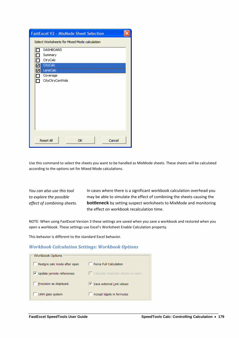
FastExcel SpeedTools User Guide SpeedTools Calc: Controlling Calculation 179
Use this command to select the sheets you want to be handled as MixMode sheets. These sheets will be calculated
according to the options set for Mixed Mode calculations.
You can also use this tool
to explore the possible
effect of combining sheets.
In cases where there is a significant workbook calculation overhead you
may be able to simulate the effect of combining the sheets causing the
bottleneck by setting suspect worksheets to MixMode and monitoring
the effect on workbook recalculation time.
NOTE: When using FastExcel Version 3 these settings are saved when you save a workbook and restored when you
open a workbook. These settings use Excel’s Worksheet Enable Calculation property.
This behavior is different to the standard Excel behavior.
WorkbookCalculationSettings:WorkbookOptions
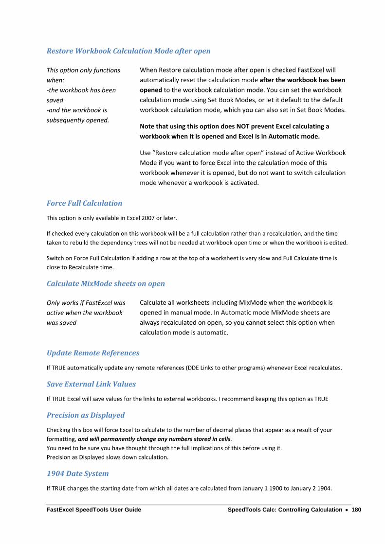
FastExcel SpeedTools User Guide SpeedTools Calc: Controlling Calculation 180
RestoreWorkbookCalculationModeafteropen
This option only functions
when:
‐the workbook has been
saved
‐and the workbook is
subsequently opened.
When Restore calculation mode after open is checked FastExcel will
automatically reset the calculation mode after the workbook has been
opened to the workbook calculation mode. You can set the workbook
calculation mode using Set Book Modes, or let it default to the default
workbook calculation mode, which you can also set in Set Book Modes.
Note that using this option does NOT prevent Excel calculating a
workbook when it is opened and Excel is in Automatic mode.
Use “Restore calculation mode after open” instead of Active Workbook
Mode if you want to force Excel into the calculation mode of this
workbook whenever it is opened, but do not want to switch calculation
mode whenever a workbook is activated.
ForceFullCalculation
This option is only available in Excel 2007 or later.
If checked every calculation on this workbook will be a full calculation rather than a recalculation, and the time
taken to rebuild the dependency trees will not be needed at workbook open time or when the workbook is edited.
Switch on Force Full Calculation if adding a row at the top of a worksheet is very slow and Full Calculate time is
close to Recalculate time.
CalculateMixModesheetsonopen
Only works if FastExcel was
active when the workbook
was saved
Calculate all worksheets including MixMode when the workbook is
opened in manual mode. In Automatic mode MixMode sheets are
always recalculated on open, so you cannot select this option when
calculation mode is automatic.
UpdateRemoteReferences
If TRUE automatically update any remote references (DDE Links to other programs) whenever Excel recalculates.
SaveExternalLinkValues
If TRUE Excel will save values for the links to external workbooks. I recommend keeping this option as TRUE
PrecisionasDisplayed
Checking this box will force Excel to calculate to the number of decimal places that appear as a result of your
formatting, and will permanently change any numbers stored in cells.
You need to be sure you have thought through the full implications of this before using it.
Precision as Displayed slows down calculation.
1904DateSystem
If TRUE changes the starting date from which all dates are calculated from January 1 1900 to January 2 1904.

FastExcel SpeedTools User Guide SpeedTools Calc: Controlling Calculation 181
AcceptLabelsinFormulas
This allows Excel to use natural language labels in formulae. Because there are circumstances when this will give
you unexpected or ambiguous results, I recommend you do NOT use this feature.

FastExcel SpeedTools User Guide SpeedTools Calc: Controlling Calculation 182
SpeedToolsSettings
CalculationTimersforbuttonsandkeys
You can control the FastExcel calculation time display separately for the calculate buttons and the calculate keys.
The calculate buttons are the buttons on the FastExcel toolbar and on the Excel Calculation Settings tab of the
FastExcel Options form.
When checked you will see a message box after the calculation showing the time taken by the calculation.
RangeCalculateSettings
RangeCalcinc/exclDependents
In Excel 2007 and later there are 2 different Range calculate methods. One includes within‐range dependency
calculations and the other ignores within‐range dependencies and calculates row by row strictly left‐to‐right and
top‐to‐bottom. Range Calculate always ignores dependencies outside the selected range, although the selected
range will be expanded to include all the cells in multi‐cell array formulae.
SetNumberofRangeCalcTrials
Because RangeCalc timing can be sensitive to Windows multi‐tasking it is better to allow a number of trials. The
Median (middle‐most) calculation time will automatically be used, thus discarding incorrectly high and low values.
You can set the number of trials: the default number is 3.

FastExcel SpeedTools User Guide SpeedTools Calc: Controlling Calculation 183
LookupMemorySettings
FastExcel SpeedTools defaults to saving the Lookup Memory data in the workbook, and restores the Lookup
Memory when the workbook opens.
If you do not want to store the Lookup Memory you can switch of the save process by un‐checking the Save
Memory with Workbook box.
If you want to force storing the Lookup Memory data externally to the workbook check the Always Store
Externally box. You can use this option in conjunction with the retrieve memory button to transfer lookup memory
between workbooks.
Clear Memory clears the currently active Lookup Memory, but does not delete it from an already saved workbook.
Count Lookup Memory shows you the number of lookup memory values by type.
Retrieve Memory tries to get Lookup Memory from the workbook, and if there is no Lookup Memory stored within
the workbook will then look for external Lookup Memory files.

FastExcel SpeedTools User Guide SpeedTools Calc: Controlling Calculation 184
SpeedToolsLicensingSettings
Show License Status shows you the status of your licenses for all SpeedTools products.
Add New License asks which product you want to add a license for:

FastExcel SpeedTools User Guide SpeedTools Calc: Controlling Calculation 185
And then prompts for the License Activation key.

FastExcel SpeedTools User Guide Using SpeedTools with VBA 186
UsingSpeedToolswithVBA
TimingUserDefinedFunctions
You can use the SpeedTools calculate range button to time the execution of User defined functions. To get
accurate results you should set the number of trials to at least 3, preferably 5.

FastExcel SpeedTools User Guide Using SpeedTools with VBA 187
UsingSpeedToolscalculationmethodsfromVBA
If you are using any of SpeedTools’s additional calculation modes and options and your VBA program is requesting
Excel calculations you should use SpeedTools’s enhanced calculation methods.
If you use Excel’s standard calculation methods either SpeedTools’s additional calculation modes and options will
not operate or you may get unexpected results.
You can access SpeedTools’s calculation methods from VBA either by using Application.Run or by setting a
reference in your VBA project to FastExcelV3_SpeedTools: Alt‐F11 to go to the VBE, then ToolsReferences and
check the box beside FastExcelV3_SpeedTools.
The available calculation methods are:
FxlRangeCalc
FxlRangeCalc calculates the selected range on the active sheet in the same way as the SpeedTools Calculate Range
button (includes special processing for Excel 2002).
FxlSheetCalc
FxlSheetCalc recalculates the selected worksheet(s) in the same way as the SpeedTools Recalculate Sheets button.
FxlFullSheetCalc
FxlFullSheetCalc full calculates the selected worksheet(s) in the same way as the SpeedTools Full Calculate Sheets
button.
FxlBookCalc
FxlBookCalc recalculates workbooks in the same way as the SpeedTools Calculate Book button.
FxlFullbookCalc
FxlFullBookTime does a full workbook calculation in the same way as the SpeedTools Full Calculate button.
FxlDisabledSheetsCalc
FxlDisabledSheetsCalc recalculates workbooks including Mixed mode worksheets.
FxlFullDependCalc(OnlyExcel2002andlater)
The workbooks will have their dependency trees rebuilt and a full calculation will be done.

FastExcel SpeedTools User Guide Using SpeedTools with VBA 188
MICROTIMERfunction
The MICROTIMER function is a wrapper function for the Windows high‐resolution timer API.
The function returns a double containing seconds. The resolution of the timer is dependent on the clock speed of
your PC, but is about 1 microsecond on a 1200MHZ AMD. The function itself takes about 5 microseconds to
execute when called from VBA on the same machine.
The function is not volatile, and is primarily designed to be called from VBA Subs/Functions rather than from a
worksheet.
MICROTIMERSyntax
MICROTIMER()
MICROTIMERRemarks
To call the function from VBA you must first make a reference from the VBE to FastExcelV3_SpeedTools:
Open the VBE (Alt F11)
Open a module within your VBA project
Tools‐>References and check FastExcelV3_SpeedTools.
It is also possible to evaluate the function from VBA as a worksheet function using Evaluate, but this incurs
significant extra overhead.
MILLITIMERfunction
The MILLITIMER function is a wrapper function for the Windows medium‐resolution timer API.
The function returns a long containing milliseconds. The resolution of the timer is about 5 milliseconds. The
function itself takes about 1 millisecond to execute when called from VBA on the same machine.
The function is not volatile, and is primarily designed to be called from VBA Subs/Functions rather than from a
worksheet.
MILLITIMERSyntax
MILLITIMER()
MILLITIMERRemarks
To call the function from VBA you must first make a reference from the VBE to FastExcelV3_SpeedTools:
Open the VBE
Open a module within your VBA project
Tools‐>References and check FastExcelV3_SpeedTools.
It is also possible to evaluate the function from VBA as a worksheet function using Evaluate, but this incurs
significant extra overhead.

FastExcel SpeedTools User Guide Using SpeedTools with VBA 189
STRCOLIDfunction
The STRCOLID function returns an alphabetic column name (A to XFD) given a column number.
STRCOLIDSyntax
STRCOLID(jColNo)
JColNo
jColNo is the number of the column you want to convert to a column name.
STRCOLIDRemarks
If the column number is greater than 16384 STRCOLID returns #N/A
STRCOLID can be used either as a worksheet function or from VBA.
The main use of STRCOLID as a worksheet function is to calculate a cell address as a string for use with INDIRECT.

FastExcel SpeedTools User Guide Using SpeedTools with VBA 190
UsingMICROTIMERfromVBA
You can call the FastExcel Microtimer function from your VBA code to get high‐resolution timings on parts of your
code.
The MICROTIMER function is a wrapper function for the Windows high‐resolution timer API.
The function returns a double containing seconds. The resolution of the timer is dependent on the clock speed of
your PC, but is about 1 microsecond on a 1200MHZ AMD. The function itself takes about 5 microseconds to
execute when called from VBA on the same machine.
SettingareferencetoFastExcelSpeedTools
Open the VBE (alt‐F11)
Select your VBA project
VBE Tools ‐‐> References
Check the box next to FastExcelV3_SpeedTools
UsingMICROTIMERincode
The Microtimer function returns a double containing time in seconds.
This example measures the time taken to recalculate workbooks including Mixed Mode worksheets.
Dim dTime1 as double
dTime1=MICROTIMER
FxlDisabledSheetsCalc
dTime1=MICROTIMER-dTime1
Msgbox “Calculate Time “ & cstr(dTime1)