Embed Size (px)
Citation preview
FAULT TOLERANCE
IN
ARTIFICIAL NEURAL
NETWORKS
Are Neural Networks Inherently Fault Tolerant?
George Ravuama Bolt
D.Phil. Thesis
University of York
Advanced Computer Architecture Group
Department of Computer Science
November 1992
ABSTRACT
This thesis has examined the resilience of artificial neural networks to the
effect of faults. In particular, it addressed the question of whether neural
networks are inherently fault tolerant. Neural networks were visualised from
an abstract functional level rather than a physical implementation level to
allow their computational fault tolerance to be assessed.
This high-level approach required a methodology to be developed for the
construction of fault models. Instead of abstracting the effects of physical
defects, the system itself was abstracted and fault modes extracted from this
description. Requirements for suitable measures to assess a neural network's
reliability in the presence of faults were given, and general measures
constructed. Also, simulation frameworks were evolved which could allow
comparative studies to be made between different architectures and models.
It was found that a major influence on the reliability of neural networks is
the uniform distribution of information. Critical faults may cause failure for
certain regions of input space without this property. This lead to new
techniques being developed which ensure uniform storage.
It was shown that the basic perceptron unit possesses a degree of fault
tolerance related to the characteristics of its input data. This implied that
complex perceptron based neural networks can be inherently fault tolerant
given suitable training algorithms. However, it was then shown that
back-error propagation for multi-layer perceptron networks (MLP's) does
not produce a suitable weight configuration.
A technique involving the injection of transient faults during back-error
propagation training of MLP's was studied. The computational factor in the
resulting MLP's causing their resilience to faults was then identified. This
lead to a much simpler construction method which does not involve lengthy
training times. It was then shown why the conventional back-error
propagation algorithm does not produce fault tolerant MLP's.
It was concluded that a potential for inherent fault tolerance does exist in
neural network architectures, but it is not exploited by current training
algorithms.
i
CONTENTS
Abstract i
Contents iiList of Figures . . . . . . . . . . . .. . . . . . . . . . . . . . . . . . . . . . . .. . . . . . . . . . . . . viii. . . . .
List of Tables . . . . . . . . . . . .. . . . . . . . . . . . . . . . . . . . . . . .. . . . . . . . . . . . . . x. . . . . .
List of Graphs. . . . . . . . . . . .. . . . . . . . . . . . . . . . . . . . . . . .. . . . . . . . . . . . . . xi. . . . . .
Acknowledgement. . . . . . . . . . . .. . . . . . . . . . . . . . . . . . . . . . . .. . . . . . . . . . xiii. . . . .
Declaration . . . . . . . . . . . .. . . . . . . . . . . . . . . . . . . . . . . .. . . . . . . . . . . . . . . . xiv. . . . .
1. Introduction 11.1. Thesis Aims. . . . . . . . . . . .. . . . . . . . . . . . . . . . . . . . . . . .. . . . . . . . . . . 1. . . . . .
1.2. Motivation . . . . . . . . . . . .. . . . . . . . . . . . . . . . . . . . . . . .. . . . . . . . . . . . 2. . . . . .
1.3. Terminology . . . . . . . . . . . .. . . . . . . . . . . . . . . . . . . . . . . .. . . . . . . . . . 2. . . . . .
1.3.1. Neural Networks. . . . . . . . . . . .. . . . . . . . . . . . . . . . . . . . . . . .. . . . 2. . . . . .
1.3.2. Reliability Theory . . . . . . . . . . . .. . . . . . . . . . . . . . . . . . . . . . . .. . 5. . . . . .
1.4. Thesis Overview. . . . . . . . . . . .. . . . . . . . . . . . . . . . . . . . . . . .. . . . . . . 6. . . . . .
1.4.1. Chapter 2: Reliable Neural Networks. . . . . . . . . . . .. . . . . . . . . . . 6. . . . . .
1.4.2. Chapter 3: Concepts. . . . . . . . . . . .. . . . . . . . . . . . . . . . . . . . . . . .. 7. . . . . .
1.4.3. Chapter 4: A Methodology for Fault Tolerance. . . . . . . . . . . .. . . 7. . . . . .
1.4.4. Chapter 5: ADAM . . . . . . . . . . . .. . . . . . . . . . . . . . . . . . . . . . . .. . 8. . . . . .
1.4.5. Chapter 6: Multi-Layer Perceptron Networks. . . . . . . . . . . .. . . . 8. . . . . .
1.4.6. Chapter 7: Conclusions. . . . . . . . . . . .. . . . . . . . . . . . . . . . . . . . . . 9. . . . . .
1.4.7. Appendix A: Fault Tolerance of Lateral Interaction Networks. . 9. . . . . .
1.4.8. Appendix B: Glossary. . . . . . . . . . . .. . . . . . . . . . . . . . . . . . . . . . . 9. . . . . .
1.4.9. Appendix C: Data from ADAM Simulations. . . . . . . . . . . .. . . . . 9. . . . . .
2. Reliable Neural Networks 102.1. Introduction . . . . . . . . . . . .. . . . . . . . . . . . . . . . . . . . . . . .. . . . . . . . . . . 10. . . . .
2.2. Frameworks for Analysing Fault Tolerance. . . . . . . . . . . .. . . . . . . . . 11. . . . .
2.2.1. Fault Models. . . . . . . . . . . .. . . . . . . . . . . . . . . . . . . . . . . .. . . . . . . 12. . . . .
2.2.2. Assessing Fault Tolerance. . . . . . . . . . . .. . . . . . . . . . . . . . . . . . . . 13. . . . .
2.2.3. Simulation Frameworks. . . . . . . . . . . .. . . . . . . . . . . . . . . . . . . . . . 15. . . . .
ii
2.3. Redundancy. . . . . . . . . . . .. . . . . . . . . . . . . . . . . . . . . . . .. . . . . . . . . . . 16. . . . .
2.3.1. Modular Redundancy. . . . . . . . . . . .. . . . . . . . . . . . . . . . . . . . . . . . 17. . . . .
2.3.2. Distributed .vs. Local Representations. . . . . . . . . . . .. . . . . . . . . . 18. . . . .
2.3.3. Input and Output Representations. . . . . . . . . . . .. . . . . . . . . . . . . . 20. . . . .
2.3.4. Computational Complexity and Capacity. . . . . . . . . . . .. . . . . . . . 21. . . . .
2.3.5. Basins of Attraction. . . . . . . . . . . .. . . . . . . . . . . . . . . . . . . . . . . .. 22. . . . .
2.4. Reliability during the Learning Phase. . . . . . . . . . . .. . . . . . . . . . . . . . 23. . . . .
2.4.1. Retraining. . . . . . . . . . . .. . . . . . . . . . . . . . . . . . . . . . . .. . . . . . . . . 24. . . . .
2.5. Fault Management. . . . . . . . . . . .. . . . . . . . . . . . . . . . . . . . . . . .. . . . . . 25. . . . .
2.6. Analysis of Specific Neural Network Models. . . . . . . . . . . .. . . . . . . . 26. . . . .
2.6.1. Hopfield Neural Network Model. . . . . . . . . . . .. . . . . . . . . . . . . . 26. . . . .
2.6.2. Multi-Layer Perceptron Model. . . . . . . . . . . .. . . . . . . . . . . . . . . . 28. . . . .
2.6.3. CMAC Networks . . . . . . . . . . . .. . . . . . . . . . . . . . . . . . . . . . . .. . . 32. . . . .
2.6.4. Compacta Networks. . . . . . . . . . . .. . . . . . . . . . . . . . . . . . . . . . . .. 33. . . . .
2.7. Fault Tolerance Techniques for Neural Networks. . . . . . . . . . . .. . . . 33. . . . .
2.8. Fault Tolerance of "Real" Neural Networks. . . . . . . . . . . .. . . . . . . . . 36. . . . .
2.9. Conclusions. . . . . . . . . . . .. . . . . . . . . . . . . . . . . . . . . . . .. . . . . . . . . . . 36. . . . .
3. Concepts 383.1. Introduction . . . . . . . . . . . .. . . . . . . . . . . . . . . . . . . . . . . .. . . . . . . . . . . 38. . . . .
3.2. Learning in Neural Networks. . . . . . . . . . . .. . . . . . . . . . . . . . . . . . . . . 39. . . . .
3.2.1. Supervised Learning. . . . . . . . . . . .. . . . . . . . . . . . . . . . . . . . . . . .. 40. . . . .
3.3. Distribution . . . . . . . . . . . .. . . . . . . . . . . . . . . . . . . . . . . .. . . . . . . . . . . 41. . . . .
3.4. Generalisation. . . . . . . . . . . .. . . . . . . . . . . . . . . . . . . . . . . .. . . . . . . . . 42. . . . .
3.4.1. Local vs. Global Generalisation. . . . . . . . . . . .. . . . . . . . . . . . . . . 43. . . . .
3.4.2. Interpolation vs. Inexact Classification. . . . . . . . . . . .. . . . . . . . . . 45. . . . .
3.4.3. Fault Tolerance as a Constraint. . . . . . . . . . . .. . . . . . . . . . . . . . . . 47. . . . .
3.5. Architectural Aspects of Neural Networks. . . . . . . . . . . .. . . . . . . . . . 49. . . . .
3.6. Failure in Neural Networks. . . . . . . . . . . .. . . . . . . . . . . . . . . . . . . . . . 50. . . . .
3.7. Problem Classification. . . . . . . . . . . .. . . . . . . . . . . . . . . . . . . . . . . .. . 51. . . . .
3.7.1. Soft Problem Domains. . . . . . . . . . . .. . . . . . . . . . . . . . . . . . . . . . . 52. . . . .
3.7.2. Considerations for Graceful Degradation. . . . . . . . . . . .. . . . . . . . 53. . . . .
3.8. Computational Fault Tolerance. . . . . . . . . . . .. . . . . . . . . . . . . . . . . . . 53. . . . .
3.9. Verifying an Adaptive System. . . . . . . . . . . .. . . . . . . . . . . . . . . . . . . . 55. . . . .
3.10. Conclusions. . . . . . . . . . . .. . . . . . . . . . . . . . . . . . . . . . . .. . . . . . . . . . 56. . . . .
iii
4. A Methodology for Fault Tolerance 574.1. Introduction . . . . . . . . . . . .. . . . . . . . . . . . . . . . . . . . . . . .. . . . . . . . . . . 57. . . . .
4.2. Fault Models . . . . . . . . . . . .. . . . . . . . . . . . . . . . . . . . . . . .. . . . . . . . . . 58. . . . .
4.3. Visualisation Levels for Neural Networks. . . . . . . . . . . .. . . . . . . . . . 59. . . . .
4.3.1. Abstract Level. . . . . . . . . . . .. . . . . . . . . . . . . . . . . . . . . . . .. . . . . . 60. . . . .
4.3.2. Role of Fault Models. . . . . . . . . . . .. . . . . . . . . . . . . . . . . . . . . . . . 61. . . . .
4.4. Conventional Fault Models. . . . . . . . . . . .. . . . . . . . . . . . . . . . . . . . . . . 61. . . . .
4.5. Fault Locations. . . . . . . . . . . .. . . . . . . . . . . . . . . . . . . . . . . .. . . . . . . . 63. . . . .
4.5.1. Fault Locations for Neural Networks. . . . . . . . . . . .. . . . . . . . . . . 64. . . . .
4.5.2. Example . . . . . . . . . . . .. . . . . . . . . . . . . . . . . . . . . . . .. . . . . . . . . . 65. . . . .
4.6. Fault Manifestations. . . . . . . . . . . .. . . . . . . . . . . . . . . . . . . . . . . .. . . . 66. . . . .
4.6.1. Example . . . . . . . . . . . .. . . . . . . . . . . . . . . . . . . . . . . .. . . . . . . . . . 68. . . . .
4.6.2. Threshold Function. . . . . . . . . . . .. . . . . . . . . . . . . . . . . . . . . . . .. 69. . . . .
4.6.3. Differential of Threshold Function. . . . . . . . . . . .. . . . . . . . . . . . . 69. . . . .
4.6.4. Weights . . . . . . . . . . . .. . . . . . . . . . . . . . . . . . . . . . . .. . . . . . . . . . . 70. . . . .
4.6.5. Topology. . . . . . . . . . . .. . . . . . . . . . . . . . . . . . . . . . . .. . . . . . . . . . 72. . . . .
4.6.6. Other Fault Locations. . . . . . . . . . . .. . . . . . . . . . . . . . . . . . . . . . . . 72. . . . .
4.7. Spatial and Temporal Considerations. . . . . . . . . . . .. . . . . . . . . . . . . . 73. . . . .
4.8. Summary . . . . . . . . . . . .. . . . . . . . . . . . . . . . . . . . . . . .. . . . . . . . . . . . . 74. . . . .
4.9. Functional Fault Models. . . . . . . . . . . .. . . . . . . . . . . . . . . . . . . . . . . .. 75. . . . .
4.10. Fault Coverage. . . . . . . . . . . .. . . . . . . . . . . . . . . . . . . . . . . .. . . . . . . . 76. . . . .
4.11. Assessing Reliability. . . . . . . . . . . .. . . . . . . . . . . . . . . . . . . . . . . .. . . 76. . . . .
4.12. Failure in Neural Networks. . . . . . . . . . . .. . . . . . . . . . . . . . . . . . . . . 77. . . . .
4.12.1. Measuring Failure. . . . . . . . . . . .. . . . . . . . . . . . . . . . . . . . . . . .. 78. . . . .
4.12.2. Applying Failure Measures. . . . . . . . . . . .. . . . . . . . . . . . . . . . . . 80. . . . .
4.12.3. Example . . . . . . . . . . . .. . . . . . . . . . . . . . . . . . . . . . . .. . . . . . . . . 81. . . . .
4.13. Relationship to Fault Tolerance. . . . . . . . . . . .. . . . . . . . . . . . . . . . . . 82. . . . .
4.14. Empirical Frameworks. . . . . . . . . . . .. . . . . . . . . . . . . . . . . . . . . . . .. 83. . . . .
4.14.1. Timescales. . . . . . . . . . . .. . . . . . . . . . . . . . . . . . . . . . . .. . . . . . . . 83. . . . .
4.14.2. Fault Injection Methods. . . . . . . . . . . .. . . . . . . . . . . . . . . . . . . . . 85. . . . .
4.14.3. Example . . . . . . . . . . . .. . . . . . . . . . . . . . . . . . . . . . . .. . . . . . . . . 86. . . . .
4.14.4. Mean-Time-Before-Failure Methods. . . . . . . . . . . .. . . . . . . . . . 87. . . . .
4.14.5. Example . . . . . . . . . . . .. . . . . . . . . . . . . . . . . . . . . . . .. . . . . . . . . 88. . . . .
4.14.6. Service Degradation Methods. . . . . . . . . . . .. . . . . . . . . . . . . . . . 89. . . . .
4.14.7. Example . . . . . . . . . . . .. . . . . . . . . . . . . . . . . . . . . . . .. . . . . . . . . 90. . . . .
4.14.8. Summary of Simulation Frameworks. . . . . . . . . . . .. . . . . . . . . . 90. . . . .
4.15. Conclusions. . . . . . . . . . . .. . . . . . . . . . . . . . . . . . . . . . . .. . . . . . . . . . 91. . . . .
iv
ADAM 925.1. Introduction . . . . . . . . . . . .. . . . . . . . . . . . . . . . . . . . . . . .. . . . . . . . . . . 92. . . . .
5.2. The ADAM System. . . . . . . . . . . .. . . . . . . . . . . . . . . . . . . . . . . .. . . . . 93. . . . .
5.2.1. Recall of Stored Vectors. . . . . . . . . . . .. . . . . . . . . . . . . . . . . . . . . 94. . . . .
5.2.2. Teaching the ADAM System. . . . . . . . . . . .. . . . . . . . . . . . . . . . . 95. . . . .
5.2.3. Memory Saturation. . . . . . . . . . . .. . . . . . . . . . . . . . . . . . . . . . . .. . 96. . . . .
5.3. Fault Tolerance. . . . . . . . . . . .. . . . . . . . . . . . . . . . . . . . . . . .. . . . . . . . 96. . . . .
5.3.1. Fault Model. . . . . . . . . . . .. . . . . . . . . . . . . . . . . . . . . . . .. . . . . . . . 97. . . . .
5.3.2. Software Simulation of Faults . . . . . . . . . . . .. . . . . . . . . . . . . . . . 98. . . . .
5.3.3. Experimental Approaches. . . . . . . . . . . .. . . . . . . . . . . . . . . . . . . . 98. . . . .
5.4. Uniform Storage in ADAM. . . . . . . . . . . .. . . . . . . . . . . . . . . . . . . . . . 100. . . .
5.4.1. Input Data. . . . . . . . . . . .. . . . . . . . . . . . . . . . . . . . . . . .. . . . . . . . . 100. . . .
5.4.2. Analysis of Bit Density on Storage. . . . . . . . . . . .. . . . . . . . . . . . . 100. . . .
5.4.3. Analysis for Tuple Storage P.d.f. . . . . . . . . . . . .. . . . . . . . . . . . . . 102. . . .
5.4.4. Input Data Independent ADAM. . . . . . . . . . . .. . . . . . . . . . . . . . . 104. . . .
5.4.5. Implications for Fault Tolerance. . . . . . . . . . . .. . . . . . . . . . . . . . . 105. . . .
5.4.6. Conclusions for Uniform Storage. . . . . . . . . . . .. . . . . . . . . . . . . . 107. . . .
5.5. Failure Prediction for Single Tuple ADAM Systems. . . . . . . . . . . .. . 107. . . .
5.5.1. Storage Distribution within a Memory Matrix. . . . . . . . . . . .. . . . 108. . . .
5.5.2. Effect of Faults. . . . . . . . . . . .. . . . . . . . . . . . . . . . . . . . . . . .. . . . . 111. . . .
5.5.3. Failure . . . . . . . . . . . .. . . . . . . . . . . . . . . . . . . . . . . .. . . . . . . . . . . . 112. . . .
5.5.4. Comparison with Empirical Results. . . . . . . . . . . .. . . . . . . . . . . . 113. . . .
5.5.5. Relation of Tuple Size to Probability of Failure. . . . . . . . . . . .. . 114. . . .
5.6. Failure Prediction for Multiple Tuple ADAM Systems. . . . . . . . . . . . 115. . . .
5.7. Fault Tolerance Analysis. . . . . . . . . . . .. . . . . . . . . . . . . . . . . . . . . . . . 116. . . .
5.7.1. Varying Number of Tuple Units. . . . . . . . . . . .. . . . . . . . . . . . . . . 117. . . .
5.7.2. Varying Number of Input Patterns. . . . . . . . . . . .. . . . . . . . . . . . . 120. . . .
5.8. Conclusions. . . . . . . . . . . .. . . . . . . . . . . . . . . . . . . . . . . .. . . . . . . . . . . 122. . . .
Graphs from Fault Analysis 124
Multi-Layer Perceptrons 1346.1. Introduction . . . . . . . . . . . .. . . . . . . . . . . . . . . . . . . . . . . .. . . . . . . . . . . 134. . . .
6.2. Construction of Training Sets. . . . . . . . . . . .. . . . . . . . . . . . . . . . . . . . . 135. . . .
6.3. Perceptron Units. . . . . . . . . . . .. . . . . . . . . . . . . . . . . . . . . . . .. . . . . . . 136. . . .
6.3.1. Fault Tolerance of Perceptron Units. . . . . . . . . . . .. . . . . . . . . . . . 137. . . .
6.3.2. Empirical Analysis. . . . . . . . . . . .. . . . . . . . . . . . . . . . . . . . . . . .. . 141. . . .
v
6.3.3. Alternative Visualisation of a Perceptron's Function. . . . . . . . . . 142. . . .
6.4. Multi-Layer Perceptrons. . . . . . . . . . . .. . . . . . . . . . . . . . . . . . . . . . . .. 143. . . .
6.4.1. Back-Error Propagation. . . . . . . . . . . .. . . . . . . . . . . . . . . . . . . . . . 144. . . .
6.4.2. Fault Model for MLP's. . . . . . . . . . . .. . . . . . . . . . . . . . . . . . . . . . . 144. . . .
6.5. Analysis of the Effect of Faults in MLP's. . . . . . . . . . . .. . . . . . . . . . . 145. . . .
6.5.1. Bipolar Thresholded Units. . . . . . . . . . . .. . . . . . . . . . . . . . . . . . . . 146. . . .
6.5.2. Binary Thresholded Units. . . . . . . . . . . .. . . . . . . . . . . . . . . . . . . . 147. . . .
6.5.3. Comparison between Data Representations. . . . . . . . . . . .. . . . . . 147. . . .
6.5.4. Conversion of Binary to Bipolar Thresholded MLP. . . . . . . . . . . 148. . . .
6.6. Fault Tolerance of MLP's. . . . . . . . . . . .. . . . . . . . . . . . . . . . . . . . . . . . 149. . . .
6.6.1. Distribution of Information in MLP's. . . . . . . . . . . .. . . . . . . . . . . 151. . . .
6.6.2. Analysis of Back-Error Propagation Learning. . . . . . . . . . . .. . . . 152. . . .
6.7. Training for Fault Tolerance. . . . . . . . . . . .. . . . . . . . . . . . . . . . . . . . . 155. . . .
6.7.1. Training with Weight Faults. . . . . . . . . . . .. . . . . . . . . . . . . . . . . . 155. . . .
6.7.2. Comparison with Clay and Sequin's Technique. . . . . . . . . . . .. . . 156. . . .
6.8. Analysis of Trained MLP. . . . . . . . . . . .. . . . . . . . . . . . . . . . . . . . . . . . 156. . . .
6.8.1. Analysis of Fault Injection Training. . . . . . . . . . . .. . . . . . . . . . . . 157. . . .
6.8.2. Comparison with MLP trained injecting unit faults. . . . . . . . . . . 159. . . .
6.8.3. New Technique for Fault Tolerant MLP's. . . . . . . . . . . .. . . . . . . 161. . . .
6.9. Results of Scaled MLP Fault Tolerance. . . . . . . . . . . .. . . . . . . . . . . . 163. . . .
6.10. Consequences for Generalisation. . . . . . . . . . . .. . . . . . . . . . . . . . . . . 166. . . .
6.11. Uniform Hidden Representations. . . . . . . . . . . .. . . . . . . . . . . . . . . . . 168. . . .
6.12. Conclusions . . . . . . . . . . . .. . . . . . . . . . . . . . . . . . . . . . . .. . . . . . . . . . 170. . . .
Conclusions 1727.1. Overview . . . . . . . . . . . .. . . . . . . . . . . . . . . . . . . . . . . .. . . . . . . . . . . . . 172. . . .
7.2. Basis for Inherent Fault Tolerance. . . . . . . . . . . .. . . . . . . . . . . . . . . . . 173. . . .
7.3. Fault Tolerance Mechanisms. . . . . . . . . . . .. . . . . . . . . . . . . . . . . . . . . 173. . . .
7.3.1. Uniform Fault Tolerance. . . . . . . . . . . .. . . . . . . . . . . . . . . . . . . . . 173. . . .
7.3.2. Modular Redundancy. . . . . . . . . . . .. . . . . . . . . . . . . . . . . . . . . . . . 174. . . .
7.3.3. Architectural Considerations in ADAM. . . . . . . . . . . .. . . . . . . . . 175. . . .
7.3.4. Learning in Multi-Layer Perceptron Networks. . . . . . . . . . . .. . . 175. . . .
7.4. Inherent Fault Tolerance?. . . . . . . . . . . .. . . . . . . . . . . . . . . . . . . . . . . . 177. . . .
7.5. Implications for Future Research. . . . . . . . . . . .. . . . . . . . . . . . . . . . . . 178. . . .
7.5.1. Generalisation. . . . . . . . . . . .. . . . . . . . . . . . . . . . . . . . . . . .. . . . . . 178. . . .
7.5.2. Internal Representations. . . . . . . . . . . .. . . . . . . . . . . . . . . . . . . . . . 179. . . .
7.5.3. Implementations. . . . . . . . . . . .. . . . . . . . . . . . . . . . . . . . . . . .. . . . 179. . . .
vi
7.5.4. Neural Fault Tolerance. . . . . . . . . . . .. . . . . . . . . . . . . . . . . . . . . . 179. . . .
A. Fault Tolerance of Lateral Interaction Networks 180A.1. Introduction . . . . . . . . . . . .. . . . . . . . . . . . . . . . . . . . . . . .. . . . . . . . . . . 180. . . .
A.2. Soft/Rigid Application Areas. . . . . . . . . . . .. . . . . . . . . . . . . . . . . . . . . 181. . . .
A.2.1. Implications for Reliability . . . . . . . . . . . .. . . . . . . . . . . . . . . . . . . 182. . . .
A.2.2. Verification . . . . . . . . . . . .. . . . . . . . . . . . . . . . . . . . . . . .. . . . . . . . 182. . . .
A.3. Lateral Inhibition . . . . . . . . . . . .. . . . . . . . . . . . . . . . . . . . . . . .. . . . . . . 183. . . .
A.3.1. Network Dynamics. . . . . . . . . . . .. . . . . . . . . . . . . . . . . . . . . . . .. . 184. . . .
A.3.2. Operational Behaviour. . . . . . . . . . . .. . . . . . . . . . . . . . . . . . . . . . . 185. . . .
A.3.3. Stabilisation. . . . . . . . . . . .. . . . . . . . . . . . . . . . . . . . . . . .. . . . . . . . 185. . . .
A.4. Fault Model . . . . . . . . . . . .. . . . . . . . . . . . . . . . . . . . . . . .. . . . . . . . . . . 186. . . .
A.4.1. Timescale . . . . . . . . . . . .. . . . . . . . . . . . . . . . . . . . . . . .. . . . . . . . . 187. . . .
A.5. Definition of Failure . . . . . . . . . . . .. . . . . . . . . . . . . . . . . . . . . . . .. . . . 187. . . .
A.5.1. System Failure. . . . . . . . . . . .. . . . . . . . . . . . . . . . . . . . . . . .. . . . . 188. . . .
A.5.2. Component Failure. . . . . . . . . . . .. . . . . . . . . . . . . . . . . . . . . . . .. . 189. . . .
A.6. Empirical Investigations. . . . . . . . . . . .. . . . . . . . . . . . . . . . . . . . . . . .. 190. . . .
A.6.1. Edge Enhancing . . . . . . . . . . . .. . . . . . . . . . . . . . . . . . . . . . . .. . . . 190. . . .
A.6.2. Neighbourhood Formation. . . . . . . . . . . .. . . . . . . . . . . . . . . . . . . . 192. . . .
A.7. Conclusions . . . . . . . . . . . .. . . . . . . . . . . . . . . . . . . . . . . .. . . . . . . . . . . 194. . . .
B. Glossary 195
C. Data from ADAM Simulations 200
References 206
vii
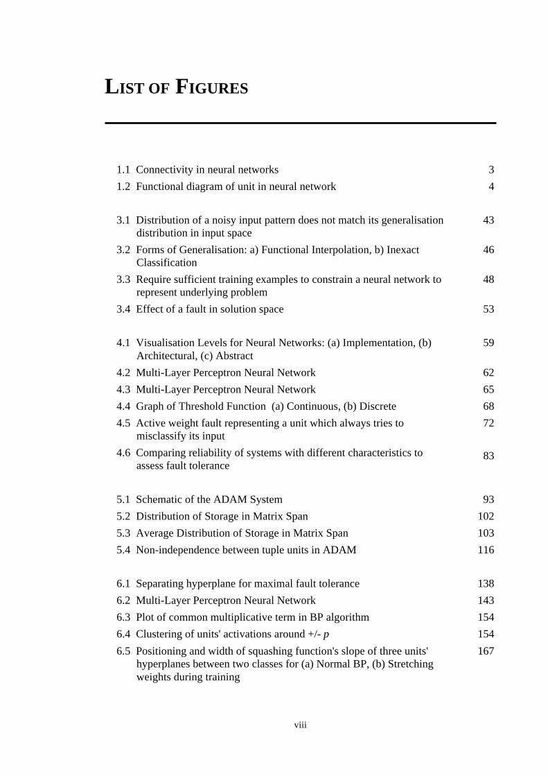
L IST OF FIGURES
1.1 Connectivity in neural networks 3
1.2 Functional diagram of unit in neural network 4
3.1 Distribution of a noisy input pattern does not match its generalisationdistribution in input space
43
3.2 Forms of Generalisation: a) Functional Interpolation, b) InexactClassification
46
3.3 Require sufficient training examples to constrain a neural network torepresent underlying problem
48
3.4 Effect of a fault in solution space 53
4.1 Visualisation Levels for Neural Networks: (a) Implementation, (b)Architectural, (c) Abstract
59
4.2 Multi-Layer Perceptron Neural Network 62
4.3 Multi-Layer Perceptron Neural Network 65
4.4 Graph of Threshold Function (a) Continuous, (b) Discrete 68
4.5 Active weight fault representing a unit which always tries tomisclassify its input
72
4.6 Comparing reliability of systems with different characteristics toassess fault tolerance
83
5.1 Schematic of the ADAM System 93
5.2 Distribution of Storage in Matrix Span 102
5.3 Average Distribution of Storage in Matrix Span 103
5.4 Non-independence between tuple units in ADAM 116
6.1 Separating hyperplane for maximal fault tolerance 138
6.2 Multi-Layer Perceptron Neural Network 143
6.3 Plot of common multiplicative term in BP algorithm 154
6.4 Clustering of units' activations around +/- p 154
6.5 Positioning and width of squashing function's slope of three units'hyperplanes between two classes for (a) Normal BP, (b) Stretchingweights during training
167
viii

A.1 Lateral interaction network, dotted lines show how weightscorrespond to Mexican-hat function
184
A.2 Lateral interaction network functions (a) Clustering, and (b) High-frequency filter (LF - Low Frequency, HF - High Frequency)
185
A.3 Faults affecting global weight vector 186
ix

L IST OF TABLES
5.1 Predicted .vs. Experimental for 2,3 and 4-Tuple Units 118
5.2 Memory saturation values when varying number of stored patterns 121
6.1 Change to fault-free activation of output unit caused by hidden unitfailure
147
C.1 Probability of failure for various numbers of 2-tuple units 200
C.2 Probability of failure for various numbers of 3-tuple units 201
C.3 Probability of failure for various numbers of 4-tuple units 202
C.4 Probability of failure for various levels of memory saturation using2-tuple units
203
C.5 Probability of failure for various levels of memory saturation using3-tuple units
204
C.6 Probability of failure for various levels of memory saturation using4-tuple units
205
x
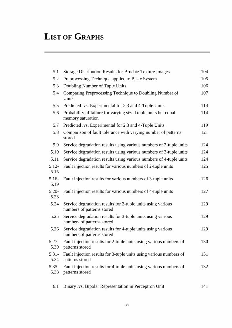
L IST OF GRAPHS
5.1 Storage Distribution Results for Brodatz Texture Images 104
5.2 Preprocessing Technique applied to Basic System 105
5.3 Doubling Number of Tuple Units 106
5.4 Comparing Preprocessing Technique to Doubling Number ofUnits
107
5.5 Predicted .vs. Experimental for 2,3 and 4-Tuple Units 114
5.6 Probability of failure for varying sized tuple units but equalmemory saturation
114
5.7 Predicted .vs. Experimental for 2,3 and 4-Tuple Units 119
5.8 Comparison of fault tolerance with varying number of patternsstored
121
5.9 Service degradation results using various numbers of 2-tuple units124
5.10 Service degradation results using various numbers of 3-tuple units 124
5.11 Service degradation results using various numbers of 4-tuple units124
5.12-5.15
Fault injection results for various numbers of 2-tuple units 125
5.16-5.19
Fault injection results for various numbers of 3-tuple units 126
5.20-5.23
Fault injection results for various numbers of 4-tuple units 127
5.24 Service degradation results for 2-tuple units using variousnumbers of patterns stored
129
5.25 Service degradation results for 3-tuple units using variousnumbers of patterns stored
129
5.26 Service degradation results for 4-tuple units using variousnumbers of patterns stored
129
5.27-5.30
Fault injection results for 2-tuple units using various numbers ofpatterns stored
130
5.31-5.34
Fault injection results for 3-tuple units using various numbers ofpatterns stored
131
5.35-5.38
Fault injection results for 4-tuple units using various numbers ofpatterns stored
132
6.1 Binary .vs. Bipolar Representation in Perceptron Unit 141
xi
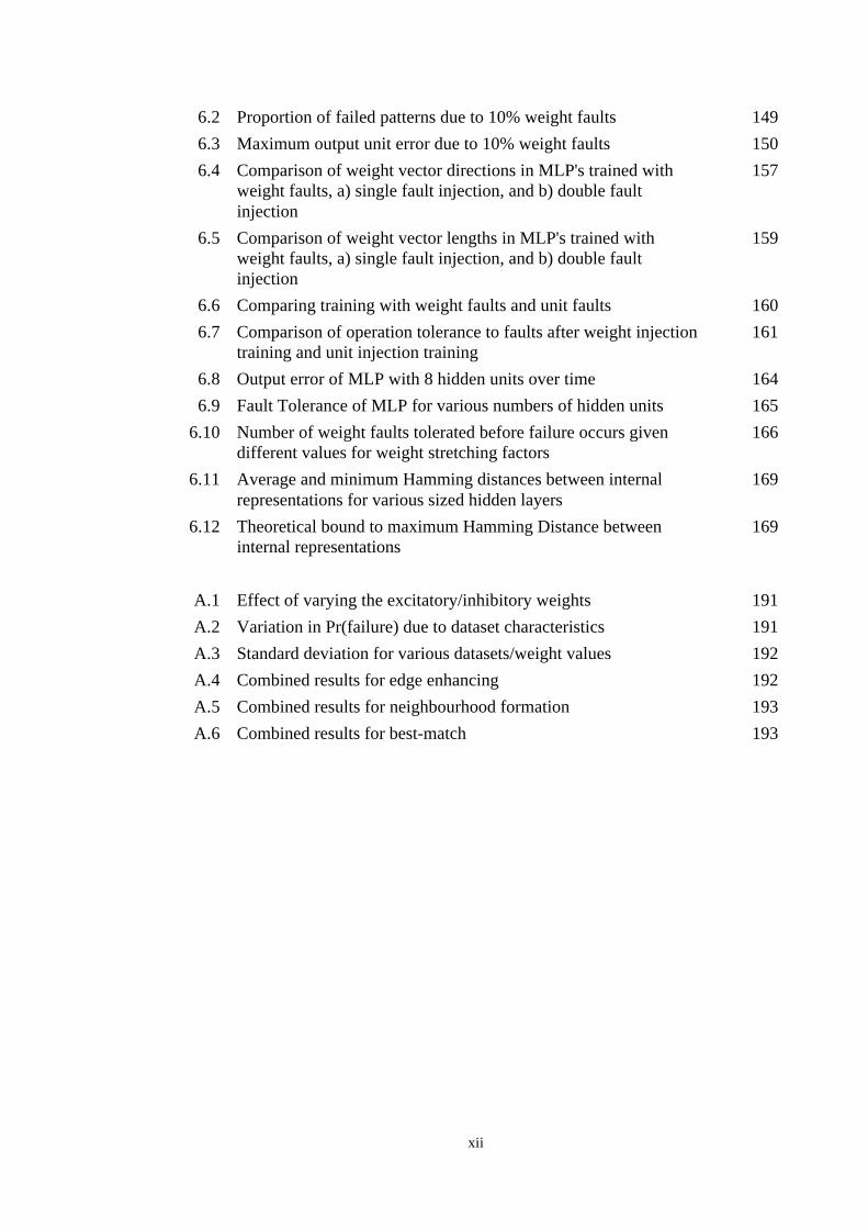
6.2 Proportion of failed patterns due to 10% weight faults 149
6.3 Maximum output unit error due to 10% weight faults 150
6.4 Comparison of weight vector directions in MLP's trained withweight faults, a) single fault injection, and b) double faultinjection
157
6.5 Comparison of weight vector lengths in MLP's trained withweight faults, a) single fault injection, and b) double faultinjection
159
6.6 Comparing training with weight faults and unit faults 160
6.7 Comparison of operation tolerance to faults after weight injectiontraining and unit injection training
161
6.8 Output error of MLP with 8 hidden units over time 164
6.9 Fault Tolerance of MLP for various numbers of hidden units 165
6.10 Number of weight faults tolerated before failure occurs givendifferent values for weight stretching factors
166
6.11 Average and minimum Hamming distances between internalrepresentations for various sized hidden layers
169
6.12 Theoretical bound to maximum Hamming Distance betweeninternal representations
169
A.1 Effect of varying the excitatory/inhibitory weights 191
A.2 Variation in Pr(failure) due to dataset characteristics 191
A.3 Standard deviation for various datasets/weight values 192
A.4 Combined results for edge enhancing 192
A.5 Combined results for neighbourhood formation 193
A.6 Combined results for best-match 193
xii

ACKNOWLEDGEME NTS
I am very grateful for the time and effort of my supervisor, Dr. James
Austin in guiding me through this D.Phil over the last three years. I also
would especially like to thank Dr. Gary Morgan for much valuable
discussion on reliability and fault tolerance mechanisms. I am indebted
to Dr. David Martland for introducing me to neural networks during my
B.Sc. at Brunel University. Many thanks to all my friends and colleagues
who have helped me at various stages. I would particularly like to thank
Mike Carter, Bruce Segee, Tom Jackson and Alan Dix for their help.
Lastly, the patience and encouragement given by my family was of great
assistance.
xiii
DECLARATION
Various parts of this thesis have been published in conference proceedings, technical
reports, and journals. These are listed below by chapter:
Chapter 3:
Bolt, G.R., "Fault Tolerance and Robustness in Neural Networks",
IJCNN-91, Seattle 2, pp.A-986 (July 1991).
Chapter 4:
Bolt, G.R., "Assessing the Reliability of Artificial Neural Networks",
IJCNN-91, Singapore 1, pp.578-583 (November 1991).
Bolt, G.R., "Fault Models for Artificial Neural Networks", IJCNN-91,
Singapore 3, pp.1918-1923 (November 1991).
Bolt, G.R., "Investigating Fault Tolerance in Artificial Neural
Networks", YCS 154, Dept. of Computer Science, University of York,
UK (March 1991).
Chapter 5:
Bolt, G.R., Austin, J. and Morgan, G., "Operational Fault Tolerance of
the ADAM Neural Network System", IEE 2nd Int. Conf. Artificial
Neural Networks, Bournemouth, pp.285-289 (November 1991).
Bolt, G.R., Austin, J. and Morgan, G., "Uniform Tuple Storage", Pattern
Recognition Letters 13, pp.339-344 (May 1992).
xiv
Chapter 6:
Bolt, G.R., Austin, J. and Morgan, G., "Fault Tolerant Multi-Layer
Perceptrons", YCS 180, Dept. of Computer Science, University of York,
UK (1992).
Appendix A:
Bolt, G.R., "Fault Tolerance of Lateral Interaction Networks",
IJCNN-91, Singapore 2, pp.1373-1378 (November 1991).
xv
CHAPTER ONE
Introduction
1.1. Thesis Aims
This thesis has two principle objectives which address the reliability of artificial neural
networks. The first will be to investigate and quantify any innate reliability which they
may possess. This will involve gaining an understanding of any existing fault tolerance
mechanisms in artificial neural networks. The second objective will be to find ways to
increase their reliability. To limit the scope of the study, only feedforward neural
networks are considered.
One of the principle questions that will be addressed in meeting the first objective is
whether neural networks are inherently fault tolerant. This property has often been
attributed to neural networks, but no sound arguments have been given to confirm or
deny it.
An essential stage in achieving the above objectives is that the consequences of inherent
or new fault tolerance mechanisms in neural networks can be analysed. Therefore, an
underlying aim will be to define a methodology for analysing the effect of faults on the
reliability of a neural network. Note that the effect of faults will only be considered at
an abstract computational level, no implementations will be analysed. This will allow a
neural network's computational fault tolerance arising from the nature of their
processing method to be understood. It will then be possible for future implementations
to be guided by this information, as well as applying conventional fault tolerance
techniques.
It is assumed that the reader has a basic knowledge of both neural networks and fault
tolerance. However, an overview will be given of the neural network models that are
examined in various chapters. For introductory texts on neural networks, see [1], [2],
Chapter 1
1
and [3]. Reliability theory (see section 1.3.2) and descriptions of various conventional
fault tolerance techniques can be found in [4], [5], and [6].
1.2. Motivation
It is important that the reliability of neural networks can be assessed since it is very
likely that the operation of potential applications will need to be ensured over some of
their lifetime. This will be especially true for safety critical systems. For instance,
neural networks appear to be well-suited for use in control systems, and it will be vital
to know the effect of faults on the system's operation. Also, very high levels of
reliability may be required for some applications. This implies that suitable fault
tolerance techniques need to be developed for neural networks to achieve this aim.
Considering the general architecture of neural networks, it is apparent that they consist
of a very large number of functionally simple components. To ensure that individual
components are reliable, it would require a very large degree of redundancy to exist.
However, this may not be cost effective or even practical in reality. However, if the
overall operation of a neural network can inherently resist the effect of such faults, then
it would imply that fault tolerance techniques need only be applied at a higher
functional level.
1.3. Terminology
This section will provide a brief overview of main terminology used in this thesis. An
extended glossary of terms is given in appendix B for reference. Various terms and
concepts will be described in the next two sections on neural networks and reliability
theory respectively.
1.3.1. Neural Networks
Neural networks provide a parallel processing environment capable of learning to solve
problems from certain domains such as pattern recognition, control of dynamical
systems, and content addressable memory. However, they are not suitable for problems
normally associated with conventional logic based computing systems, such as
performing rapid arithmetic operations.
Chapter 1
2
A neural network's architecture consists of many processing units possessing very
simple computational abilities, their inputs and output being either a discrete or
continuous scalar value. The connectivity between units is unidirectional, but often
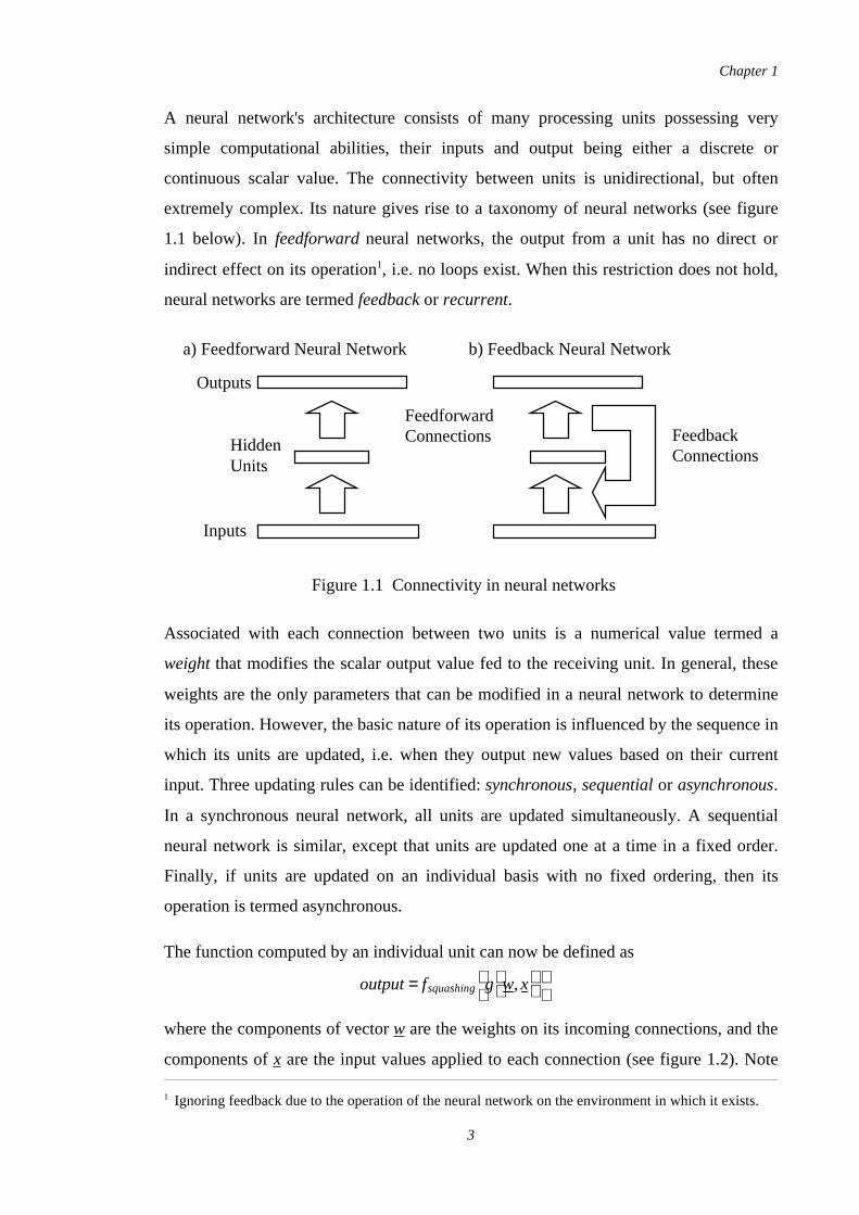
extremely complex. Its nature gives rise to a taxonomy of neural networks (see figure
1.1 below). In feedforward neural networks, the output from a unit has no direct or
indirect effect on its operation1, i.e. no loops exist. When this restriction does not hold,
neural networks are termed feedback or recurrent.
Associated with each connection between two units is a numerical value termed a
weight that modifies the scalar output value fed to the receiving unit. In general, these
weights are the only parameters that can be modified in a neural network to determine
its operation. However, the basic nature of its operation is influenced by the sequence in
which its units are updated, i.e. when they output new values based on their current
input. Three updating rules can be identified: synchronous, sequential or asynchronous.
In a synchronous neural network, all units are updated simultaneously. A sequential
neural network is similar, except that units are updated one at a time in a fixed order.
Finally, if units are updated on an individual basis with no fixed ordering, then its
operation is termed asynchronous.
The function computed by an individual unit can now be defined as
where the components of vector w are the weights on its incoming connections, and the
components of x are the input values applied to each connection (see figure 1.2). Note
1 Ignoring feedback due to the operation of the neural network on the environment in which it exists.
Outputs
HiddenUnits
Inputs
FeedforwardConnections Feedback
Connections
a) Feedforward Neural Network b) Feedback Neural Network
Figure 1.1 Connectivity in neural networks
output = fsquashingg
w,x
Chapter 1
3
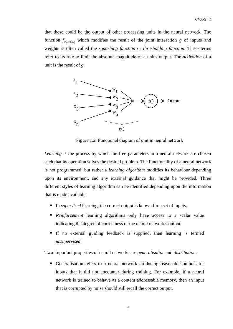
that these could be the output of other processing units in the neural network. The
function fsquashing which modifies the result of the joint interaction g of inputs and
weights is often called the squashing function or thresholding function. These terms
refer to its role to limit the absolute magnitude of a unit's output. The activation of a
unit is the result of g.
Learning is the process by which the free parameters in a neural network are chosen
such that its operation solves the desired problem. The functionality of a neural network
is not programmed, but rather a learning algorithm modifies its behaviour depending
upon its environment, and any external guidance that might be provided. Three
different styles of learning algorithm can be identified depending upon the information
that is made available.
In supervised learning, the correct output is known for a set of inputs.
Reinforcement learning algorithms only have access to a scalar value
indicating the degree of correctness of the neural network's output.
If no external guiding feedback is supplied, then learning is termed
unsupervised.
Two important properties of neural networks are generalisation and distribution:
Generalisation refers to a neural network producing reasonable outputs for
inputs that it did not encounter during training. For example, if a neural
network is trained to behave as a content addressable memory, then an input
that is corrupted by noise should still recall the correct output.
x1
x2
x3
xn
w1
w2w
3w
n
g()
f () Output
Figure 1.2 Functional diagram of unit in neural network
Chapter 1
4
During learning, the presentation of any input can potentially result in the
modification of any neural network parameter. This is often termed
information distribution. During operation, all elements in a neural network
are involved in processing an input, and this been described as distribution of
processing.
Other terminology relating to neural networks can be found in appendix B.
1.3.2. Reliability Theory
Reliability is defined as the probability that a system is still operating correctly, i.e.
according to its specification, at time t given that it was correct at time t=0. When the
operation of a system no longer meets its specification a failure is deemed to have
occurred.
The reliability of a system can be decreased due to various factors such as incorrect
operation of system components, noise affecting inputs, design inaccuracy, and change
of environment. These influences can all be viewed as faults. More formally, a fault can
be defined as the cause of errors in a system's computation, where an error is that part
in the state of a system that is likely to lead to failure. The particular class of faults
which is of interest in this thesis are those due to the physical failure of components
within a system.
However, physical defects cannot be considered directly in any analysis due to
modelling issues such as complexity and computational cost. This results in the
requirement for a fault model to be developed. It supplies a high level representation of
the effect of faults on the operation of a system's components. Associated with each
fault is a failure rate which is defined as the proportion of components that are likely to
fail over a unit period of time, i.e. describes the rate at which they become defective.
These failure rates allow the occurrence of a variety of faults in a system to be
realistically simulated, provided that the failure rate is accurately known.
One approach for improving the reliability of a system is by increasing the resilience of
its operation to the effect of faults. Methods which perform this task are termed fault
tolerance techniques. Generally such methods act by increasing the redundancy in a
system. Two types of redundancy exist: Spatial and Temporal. The former refers to
Chapter 1
5
duplicating the function of groups of physical components, which results in increasing a
system's computational capacity. The technique of N-modular redundancy (NMR) is a
good example. The latter type of redundancy involves solving a sub-problem many
times and using the results to construct some form of average final solution.
Another property of a system often resulting from the application of fault tolerance
techniques is known as graceful degradation. It can also be inherent within the system
itself. For example, the storage capacity of a memory device merely decreases as
portions of its memory space are lost. Graceful degradation can be defined to be the
ability of a system to provide useful service in the presence of faults.
1.4. Thesis Overview
This section will describe the contents of each chapter in this thesis. Various concepts
for fault tolerance in neural networks are discussed in chapter 3, and the central theme
of studying computational fault tolerance proposed. Chapter 4 supplies a methodology
for investigating fault tolerance in neural networks which is used in investigating two
neural network paradigms, ADAM (chapter 5) and multi-layer perceptrons (chapter 6).
The concept of requiring distribution in the form of producing uniform fault tolerance is
identified as crucial to developing fault tolerant neural networks.
The contents of each chapter will now be given in more detail. An extended glossary is
provided in appendix B which describes the various technical terms used in this thesis.
1.4.1. Chapter 2: Reliable Neural Networks
Chapter 2 presents a review and critique of known past and current research which
either directly or indirectly considers the effect of faults in neural networks. Work
relating to the construction of methodologies for investigating fault tolerance is
considered first. The requirement for a sound methodology is important since it
provides a basis for rigourous research and will allow meaningful comparisons to be
made between results obtained from various neural network models.
Next, various proposed computational concepts in neural networks that promote fault
tolerance will be discussed. Such concepts include distribution of information and
processing, resilience of learning algorithms to faults, and re-learning to recover from
Chapter 1
6
the effect of faults. The related problems of fault detection, location and recovery will
also be included.
There exists a considerable number of empirical investigations into the fault tolerance
of various neural network models. Work relating to the various models will be
described separately. Particular attention will be paid to whether there is any evidence
of neural networks possessing any inherent fault tolerance.
Finally, various methods that are claimed to improve the fault tolerance of certain
neural network models will be described. The relevance of examining the fault
tolerance of artificial neural networks as opposed to that of their implementation will be
considered.
1.4.2. Chapter 3: Concepts
This chapter will discuss the consequences of various features arising from the style of
computation performed by neural network on their fault tolerance and other related
properties. The features include learning, distribution of information and processing,
generalisation, and various architectural characteristics. It will also be discussed how
requiring fault tolerant operation can be viewed as a learning constraint to induce
generalisation in a neural network.
The notion of how failure occurs in a neural network will then be considered, and
contrasted to that which occurs in conventional computational systems. The related
concept of graceful degradation in neural networks will also be discussed. Following
this, a classification of problems will be proposed which is based on the nature of their
solution space. This is then used to explain how graceful degradation occurs in neural
networks.
Finally, the idea of computational fault tolerance will be introduced, and contrasted to
the more conventional physical fault tolerance. Reasons for studying neural networks at
such an abstract level are also given.
1.4.3. Chapter 4: A Methodology for Fault Tolerance
Chapter 4 will present a methodology for investigating the fault tolerance of neural
networks. This is required to provide a common baseline that will allow results between
Chapter 1
7
various neural network models, architectures, etc. to be contrasted. The chapter will
first consider how a fault model can be constructed from an abstract definition of a
neural network. The two basic steps in this process will be described, and an example
given to demonstrate its use. Various concepts relating to the application of fault
models will then considered.
The second part of the chapter will examine how the fault tolerance of neural networks
can be assessed. Finally, various simulation frameworks will be defined which allow
empirical results to be obtained.
1.4.4. Chapter 5: ADAM
This chapter will examine the fault tolerance of a binary weighted neural network
system called ADAM. After describing the neural network's architecture, training and
operation, a fault model will be constructed following the methodology to be given in
chapter 4.
The first area that will be examined is the effect on fault tolerance arising from the
storage distribution properties of tuple units. It will be shown that fault tolerance can be
improved by a new technique which ensures uniform storage. Empirical simulations
will be given which support this. A prediction model will then be constructed for the
fault tolerance of tuple units.
Finally, the fault tolerance of the first stage of ADAM will be analysed, and
comprehensive empirical simulations described and results given.
1.4.5. Chapter 6: Multi-Layer Perceptron Networks
Chapter 6 examines the fault tolerance of perceptron units and the more complex
multi-layer perceptron neural networks. First, the number of defective input
connections a single perceptron unit can tolerate is determined in terms of its input data
characteristics. This gives rise to an alternative visualisation technique for a perceptron
unit's operation.
The fault tolerance of multi-layer perceptron networks is then examined, and found to
be very sensitive to relatively few numbers of weight faults. A technique involving
transient fault injection which has been shown to improve fault tolerance is then
Chapter 1
8
analysed. This leads to an understanding of the underlying mechanisms which allow
fault tolerant multi-layer perceptron networks to be developed. Finally, empirical
simulations are carried out investigating the operational fault tolerance of multi-layer
perceptron networks created using these new construction techniques.
1.4.6. Chapter 7: Conclusions
This chapter draws together the results found in preceding chapters and discusses the
mechanisms in neural networks leading to fault tolerance. The question of whether
neural networks are inherently fault tolerant is at least partially answered.
Finally, avenues for future work extending the research presented in this thesis are
given.
1.4.7. Appendix A: Fault Tolerance of Lateral Interaction Networks
An empirical study of the fault tolerance of single layer neural networks with lateral
connections between units is presented in appendix A. It is given as an example of how
the degree of failure in a neural network can be assessed from a specification of its
functionality, rather than by using a test set of data. This is one of the concepts
described in chapter 4.
1.4.8. Appendix B: Glossary
An extended glossary of terms relating to neural networks and reliability theory are
given.
1.4.9. Appendix C: Data from ADAM Simulations
Data from simulations probing the reliability of ADAM are given.
Chapter 1
9
CHAPTER TWO
Reliable Neural Networks
2.1. Introduction
Until recently, there have been few major pieces of work which study the field of fault
tolerant neural networks, or their reliability. Early papers or technical reports tended
either to contain a passing comment that fault tolerance existed, a general discussion of
fault tolerance, or very basic experimental results of the effects of noise or faults in
neural networks [7,8,9,10,11,12,13,14,15,16,17,18]. A common misunderstanding was
confusing resilience to faults with robustness to noisy inputs. Over the last two years
though, more substantial investigations of the fault tolerance of neural networks have
been published, though there is still very little theoretical work. Overall no common
consensus exists on how to investigate the reliability of neural networks and the result
of applying fault tolerance techniques, and so the vast majority of work tends to be
rather fragmented.
Various methodologies for investigating fault tolerance will be reviewed in section 2.2,
including the definition of fault models (section 2.2.1), reliability measures used to
assess fault tolerance (section 2.2.2). The concept of redundancy, which is central to
developing fault tolerant systems, will be examined in section 2.3. It will be considered
in terms of the internal and external representations employed by neural networks
(section 2.3.2 and 3), computational learning theory concepts (section 2.3.4), and basins
of attraction (section 2.3.5). Literature concerning various other concepts arising from
the style of computation in neural networks will then be examined. This includes
training algorithm's resilience to faults and relearning in section 2.4, and fault
detection/location/recovery in section 2.5. The results from investigations into various
neural network models will be discussed in section 2.6, and conclusions drawn as to the
current ideas on fault tolerance in neural networks. The question of whether neural
networks have inherent fault tolerance will especially be concentrated on. Section 2.7
Chapter 2
10
examines various techniques for developing fault tolerance in neural networks. Finally,
section 2.8 discusses the relevance of examining the fault tolerance of neural network
implementations as opposed to the computational fault tolerance of artificial neural
networks.
2.2. Frameworks for Analysing Fault Tolerance
A requirement exists for a methodology which directs the analysis of the fault tolerance
and reliability of neural networks (c.f. chapter 4). It should consider areas such as the
construction of fault models, methods of assessing fault tolerance, and simulation
techniques to probe fault tolerance.
These requirements have also has been noted by Carter [19]. This paper is by far the
most wide-ranging published work on the notion of fault tolerance in neural networks,
although it is understandably far from comprehensive. The scope is limited to
"applications of pattern recognition and signal processing", recognising that neural
network systems which solve optimisation problems are qualitatively different to those
solving function evaluation problems. To distinguish between classical terminology
where the generally accepted definition of fault tolerance is the notion that a system
provides "error-free computation in the presence of faults", Carter uses the term
"robust" to describe a neural network since they only ever give approximate solutions
[14]. However, this change in terminology does not occur in later publications due to
confusion when it is used to describe resilience to noise affecting inputs. A very
significant distinction with respect to analysing fault tolerance is drawn between the
two phases of neural network application: training and operation. The effects of faults
are likely to be different during these two distinct periods in a neural network's
lifecycle. Carter also identifies implementation-specific fault tolerance to be another
area for separate analysis. However, this seems to be an incorrect partitioning for the
analysis of reliability in neural networks since the implementation method used is quite
likely to affect very differently the fault tolerant properties of neural networks during
the operational and training phases. For example, the weights of connections are only
changed during the learning cycle, and so the method used in the implementation for
weight alteration will lead to reliability issues that are only appropriate during this
cycle. Also, it does not take into account systems which continuously adapt during
Chapter 2
11
actual operation. Although Carter's paper considers many questions for the development
of a methodology to study the fault tolerance of neural networks, it does not provide
any specific techniques which could be used in such an analysis.
2.2.1. Fault Models
These are a model of the effect of physical faults on the operation of a system (c.f.
chapter 4). The faults in the model are generally abstract descriptions of the effects of
physical defects for reasons of computational simplicity and cost. The fault model can
then be used in empirical simulations and theoretical analysis of the system, such as
examining its fault tolerance. However, no technique is known to exist for the
construction of fault models for artificial neural networks viewed at an abstract level,
although many such studies have been made of their fault tolerance.
The fault model employed by Bedworth and Lowe [20] in their investigation of the
multi-layer perceptron network (MLP) [21] was based on physical defects of the
components required by plausible implementation methods. This contrasts with trying
to abstract faults from the description of the MLP itself. For example, linear weight
noise was compared to the effects of thermal fluctuations, non-linear weight noise due
to capacitive type errors introduced by crosstalk. Belfore and Johnson [22] examined an
implementation of Hopfield networks using an electrical neuron model. Based on the
implementation level faults that would occur in this model, more abstract faults were
defined using the stuck-at class. However, with this method it is very likely that some
faults could not be so easily abstracted due to the difference in visualisation levels, and
indeed for a particular fault "a special simulation option was implemented to model
[this fault]."
However, in the vast majority of literature no justification is given for the fault types
defined, and generally only the basic processing unit is selected as the component that
can become defective by becoming stuck at some output value. It will be shown in
chapter 4 that this is not a suitable choice due to the existence of simpler components at
this abstract level of visualisation which give rise to a more realistic and accurate fault
model.
Chapter 2
12
2.2.2. Assessing Fault Tolerance
To measure the reliability due to the fault tolerance of a neural network when operating
as an associative memory or classification system, a common technique is to evaluate
the sample probability that a pattern will be recalled correctly [23,22,24] for various
fault levels. Conversely, for function approximation a continuous measure of deviation
from correct evaluation is more appropriate [25,26]. A similar approach to evaluating
the outcome of a neural network solving an optimisation problem is given in [27].
However, these measures only assess the reliability of a neural network for each
particular instance of fault distribution, rather than describing the actual resilience of
the neural network's operation to faults. The fault tolerance of a neural network is
indicated by a curve describing the neural network's reliability of operation over a range
of fault levels.
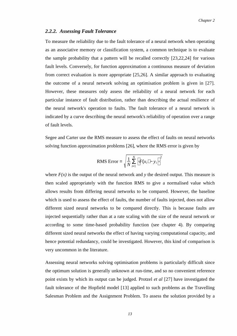
Segee and Carter use the RMS measure to assess the effect of faults on neural networks
solving function approximation problems [26], where the RMS error is given by
where F(x) is the output of the neural network and y the desired output. This measure is
then scaled appropriately with the function RMS to give a normalised value which
allows results from differing neural networks to be compared. However, the baseline
which is used to assess the effect of faults, the number of faults injected, does not allow
different sized neural networks to be compared directly. This is because faults are
injected sequentially rather than at a rate scaling with the size of the neural network or
according to some time-based probability function (see chapter 4). By comparing
different sized neural networks the effect of having varying computational capacity, and
hence potential redundancy, could be investigated. However, this kind of comparison is
very uncommon in the literature.
Assessing neural networks solving optimisation problems is particularly difficult since
the optimum solution is generally unknown at run-time, and so no convenient reference
point exists by which its output can be judged. Protzel et al [27] have investigated the
fault tolerance of the Hopfield model [13] applied to such problems as the Travelling
Salesman Problem and the Assignment Problem. To assess the solution provided by a
RMSError = 1N Σ
i=1
N F(xi) − yi
2
Chapter 2
13
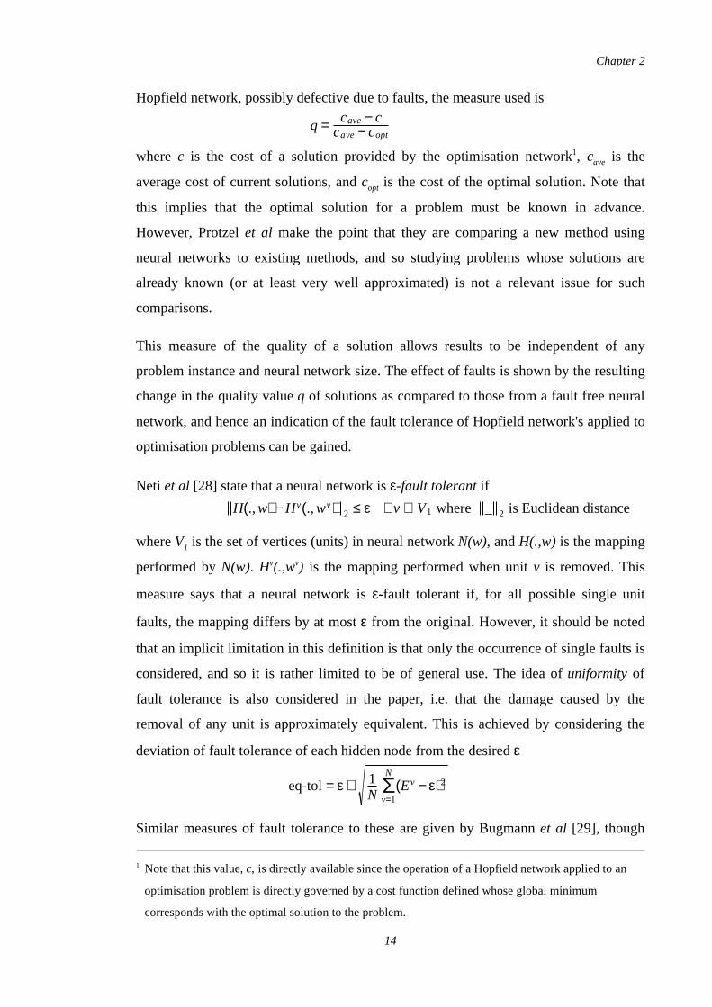
Hopfield network, possibly defective due to faults, the measure used is
where c is the cost of a solution provided by the optimisation network1, cave is the
average cost of current solutions, and copt is the cost of the optimal solution. Note that
this implies that the optimal solution for a problem must be known in advance.
However, Protzel et al make the point that they are comparing a new method using
neural networks to existing methods, and so studying problems whose solutions are
already known (or at least very well approximated) is not a relevant issue for such
comparisons.
This measure of the quality of a solution allows results to be independent of any
problem instance and neural network size. The effect of faults is shown by the resulting
change in the quality value q of solutions as compared to those from a fault free neural
network, and hence an indication of the fault tolerance of Hopfield network's applied to
optimisation problems can be gained.
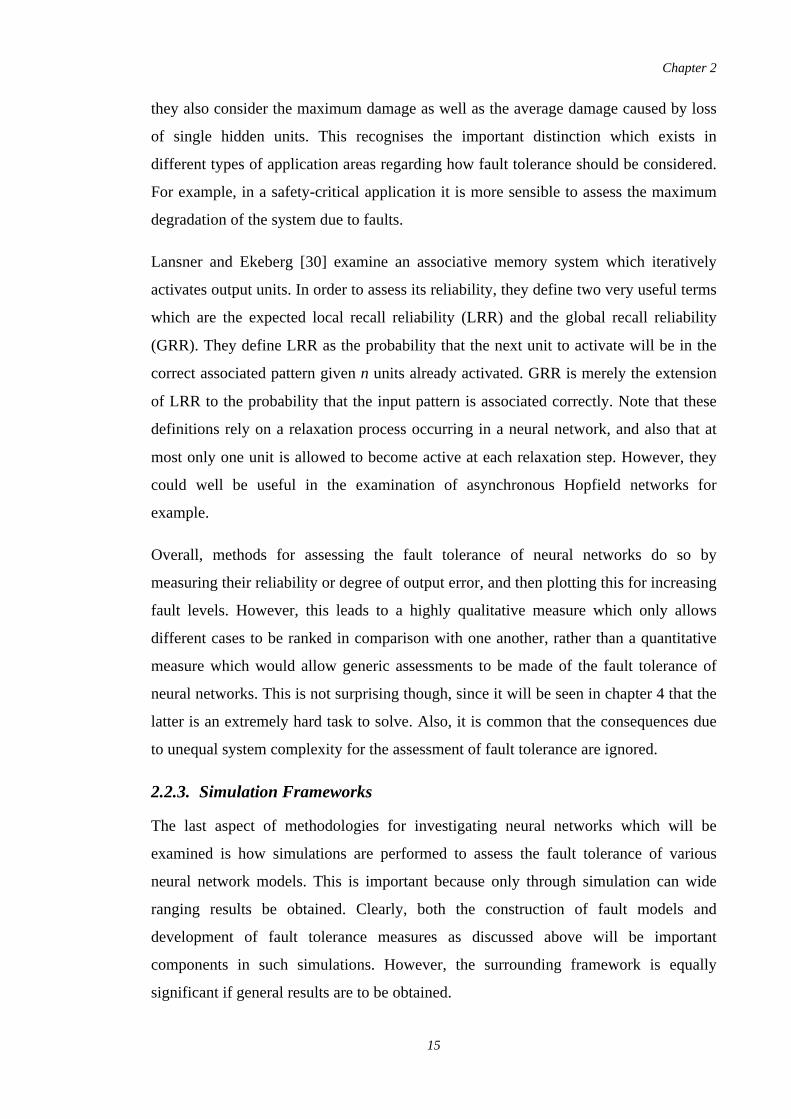
Neti et al [28] state that a neural network is ε-fault tolerant if
where V1 is the set of vertices (units) in neural network N(w), and H(.,w) is the mapping
performed by N(w). Hv(.,wv) is the mapping performed when unit v is removed. This
measure says that a neural network is ε-fault tolerant if, for all possible single unit
faults, the mapping differs by at most ε from the original. However, it should be noted
that an implicit limitation in this definition is that only the occurrence of single faults is
considered, and so it is rather limited to be of general use. The idea of uniformity of
fault tolerance is also considered in the paper, i.e. that the damage caused by the
removal of any unit is approximately equivalent. This is achieved by considering the
deviation of fault tolerance of each hidden node from the desired ε
Similar measures of fault tolerance to these are given by Bugmann et al [29], though
1 Note that this value, c, is directly available since the operation of a Hopfield network applied to an
optimisation problem is directly governed by a cost function defined whose global minimum
corresponds with the optimal solution to the problem.
q = cave − ccave − copt
H(.,w) −Hv(.,wv) 2 ≤ ε ∀ v ∈ V1 where _ 2 is Euclidean distance
eq-tol = ε ∗ 1N Σ
v=1
N
(Ev −ε)2
Chapter 2
14
they also consider the maximum damage as well as the average damage caused by loss
of single hidden units. This recognises the important distinction which exists in
different types of application areas regarding how fault tolerance should be considered.
For example, in a safety-critical application it is more sensible to assess the maximum
degradation of the system due to faults.
Lansner and Ekeberg [30] examine an associative memory system which iteratively
activates output units. In order to assess its reliability, they define two very useful terms
which are the expected local recall reliability (LRR) and the global recall reliability
(GRR). They define LRR as the probability that the next unit to activate will be in the
correct associated pattern given n units already activated. GRR is merely the extension
of LRR to the probability that the input pattern is associated correctly. Note that these
definitions rely on a relaxation process occurring in a neural network, and also that at
most only one unit is allowed to become active at each relaxation step. However, they
could well be useful in the examination of asynchronous Hopfield networks for
example.
Overall, methods for assessing the fault tolerance of neural networks do so by
measuring their reliability or degree of output error, and then plotting this for increasing
fault levels. However, this leads to a highly qualitative measure which only allows
different cases to be ranked in comparison with one another, rather than a quantitative
measure which would allow generic assessments to be made of the fault tolerance of
neural networks. This is not surprising though, since it will be seen in chapter 4 that the
latter is an extremely hard task to solve. Also, it is common that the consequences due
to unequal system complexity for the assessment of fault tolerance are ignored.
2.2.3. Simulation Frameworks
The last aspect of methodologies for investigating neural networks which will be
examined is how simulations are performed to assess the fault tolerance of various
neural network models. This is important because only through simulation can wide
ranging results be obtained. Clearly, both the construction of fault models and
development of fault tolerance measures as discussed above will be important
components in such simulations. However, the surrounding framework is equally
significant if general results are to be obtained.
Chapter 2
15
Most work examines the fault tolerance of various neural network models by
sequentially injecting faults, and examining their effect at each stage
[16,20,22,24,27,31,32,33]. This approach suffers from two deficits. First, it does not
allow the comparison of different sized neural networks since a large network will
suffer more faults than a smaller version over some fixed time period. Secondly, fault
injection techniques do not allow multiple faults to be examined in conjunction with
each other. The various faults' effects may well interact with each other, especially in
large neural networks, and so examining the effects of each fault individually will not
give an accurate picture of their combined effect in an implemented system. Prater and
Morley avoid this problem in their investigations [34] by only concentrating on the
effects of single faults. The necessity of considering the effect of multiple fault types is
neglected.
However, Segee and Carter [26] use a similar fault simulation method to May and
Hammerstrom [35] which is based on fault injection, differing only in that at each step,
the fault causing the worst damage is injected. This method overcomes the problem of
not simulating multiple differing faults occurring, but does not, as is recognised by
Segee and Carter [26], guarantee that the overall worst sequence of faults is generated.
This is since the effect of a fault which does not cause much damage when it first
occurs, could become much worse given the occurrence of some subsequent fault.
In chapter 4, various other frameworks will be suggested which allow the problems
associated with simulating the effects of multiple fault types to be overcome.
2.3. Redundancy
Redundancy of neural network components has often been identified as the factor
producing a reliable system, which corresponds with fault tolerance techniques applied
in conventional digital systems [4,6]. Moore [36] compares such conventional
techniques used to introduce fault tolerance into a computer system with apparent
mechanisms in biological neural networks, and then draws various conclusions from
this. He points out that biological networks use both spatial and temporal redundancy
(in relation to components and input/output representations), as do conventional
computing systems to achieve a greater degree of fault tolerance. However, von Seelen
and Mallot [37] question whether redundancy really is the key issue in determining the
Chapter 2
16
reliability of a neural network. They say, very plausibly, that a neural network does not
have redundancy in the sense of reserve capacity, but rather it utilises all of its resources
to gain the best trade-off between accuracy and computation time. Fault tolerance
comes from "isomorphic implementation, natural representation, a small number of
computation steps, and a balanced utilization of all available resources." [37]. By
isomorphic implementation, they mean that the output of the neural network can be
directly related to the internal processing within the network. However, though this is
reasonable for simple neural networks such as the Hopfield model where a clear
trajectory is followed through state space, for more complex models it does not seem to
be quite such a valid claim. Also, a natural representation is often a redundant signal in
its own right (e.g. retina image), so some of the influences on fault tolerance in neural
networks that they identify are not completely justified.
An interesting statement is made by McCulloch [38], "The reliability you can buy with
redundancy of calculation cannot be bought with redundancy of code or of channel".
This is in agreement with the work of von Neumann [39]. This type of redundancy
moves beyond the simple duplication of units/weights or small modules within a neural
network. It considers the possibility of inherent fault tolerance existing due to the
computational nature of neural networks introducing redundancy of calculation. For
example, temporal redundancy as often occurs in biological systems where calculations
are continuously repeated [36] can be viewed in this context.
2.3.1. Modular Redundancy
As well as redundancy of units and connections, it can also exist at higher level in terms
of groups of units or sub-networks. For instance, Izui and Pentland [40] replicate
hidden units to provide redundancy which they claim improves fault tolerance.
However, since more faults would occur in the larger neural network over a fixed time
period, this result would need more careful consideration before it could be accepted.
For similar reasons, the work by Clay and Sequin on duplication of hidden nodes also
needs further analysis [41].
At a higher level, Lincoln and Skrzypek [42] consider having many separate hidden
layers feeding into the output units, with each output acting in a similar fashion to the
judging elements in N-Modular Redundancy systems [4]. Each hidden layer is trained
Chapter 2
17
separately to solve the problem, and then all are clustered together to form the final
system. However, it is again not clear whether increased reliability is achieved despite
the increased size of the system.
The implementation of neural networks has given rise to various architectures whose
design introduces a degree of redundancy [43,44,45]. For example, a mixture of spatial
and temporal redundancy together with coding has been used by Chu and Wah [43] to
achieve a fault tolerant neural network system. Such designs make use of the regular
architectural and computational structure of neural networks to achieve redundancy.
2.3.2. Distributed .vs. Local Representations
The formation of distributed representations is often presented as a mechanism to
develop fault tolerant neural networks [8,16], though Biswas and Venkatesh take a
more pragmatic view [46] by terming such general statements as "folk theorems". They
point out that local representations lead to the existence of critical units whose failure
results in the impaired computational ability of the whole neural network. However,
they do acknowledge that evidence does exist for distributed representations which lead
to redundancy.
Baum et al examine the consequences for fault tolerance of various local and distributed
representations in an associative memory system [9]. A unary representation (relates to
the concept of Grandmother Cells) with simple replication is shown to provide a robust
associative memory system with excellent retrieval properties, though its storage
capacity is very limited. They also point out that the unary representation gives rise to
fault intolerance, although redundancy can be introduced by duplicating the
grandmother units. This is similar to ideas applied in Legendy's compacta networks
[15]. However, the claim of fault intolerance is not completely true since redundancy
will still occur in the connections feeding each grandmother unit. Faults affecting the
connections may well not cause a sufficiently large change in the unit's internal state to
alter the outcome of the winner-take-all process.
As an alternative, Baum et al [9] examine a distributed representation which is formed
by an intermediate layer of units in a layered neural network. They stress that such a
representation must not be simply several unary representations combined together
where individual units in the hidden layer still respond to only one stored pattern.
Chapter 2
18
Instead it must be truly distributed in the sense that units in the hidden layer respond to
several stored patterns, though this overlap must be controlled to minimise interference.
They then go on to consider the effect on reliability of faults causing a proportion of
input bits to be forced to zero, and for a particular training algorithm, derive the
resulting memory capacity given a required output accuracy. It is pointed out that the
redundancy introduced by the distributed representation is balanced by the need for
connection weights to take more than simply one of two states. They also point out that
sparsification of the internal representation improves the memory capacity still further,
though it is likely that this reduces the fault tolerance due to the movement towards a
unary representation. A compromise clearly exists between fault tolerance and the
capacity of the neural network arising from the chosen internal representation. This has
many similarities with the ADAM system [47] where a sparse data representation is
created using tuple units, and a distributed intermediate representation is used for
association.
The nature of the representation created by the brain-state-in-a-box model (BSB) [48] is
considered by Anderson [8]. The units in this neural network model are interconnected
via a positive feedback loop with limits placed on their absolute output values. This
produces a neural network which acts as an associative memory. Anderson suggests that
the system might well be useful as a preprocessor for noisy input data due to its
auto-associative properties. Wood [49] has carried out simulations of faults occurring in
the feedback matrix, and found that the results lead to a mixed conclusion. Although a
gradual decrease in accuracy of recall as faults occur might be expected from statistical
predictions, the results showed that as well as distributed representations, localisation
also existed which lead to critical connections. It can be concluded that it would be very
useful to have a measure which indicates the degree of the information distribution in a
neural network.
Anderson [8] has also differentiated between unary and distributed representations by
considering feature detectors which consist of either one neuron (microfeature) or
several (macrofeature). The vector feature model employs lateral excitation based on
the cerebral cortex, which results in several units behaving as a feature group. However,
this is not a distributed representation as defined by Baum et al above, and this may be
the reason for the rather mixed results which Wood found, as described above.
Chapter 2
19
2.3.3. Input and Output Representations
As well as distributed internal representations leading to a more reliable neural network,
the same can also be said for the input and output representation used [36,51]. Such
distribution leads to redundancy, for example, overlapping groups of output units where
each represents a particular classification. Methods for forming distributed
representations are discussed by Miikkulainen and Dyer [52], and include extending the
back-error propagation algorithm [21] to modify the input vectors passed to the neural
network. They found that the final neural network was fault tolerant to damage in its
input layer of units due to the learned distributed representation, and also that it
degraded in an approximately linear manner. However, the system requires a lexicon to
map actual "world" input vectors to the distributed input vector the neural network
requires, and this could become the keystone for the reliability of the overall system.
Various input representations for numerical values are considered by Takeda and
Goodman [53], such as either a binary and simple sum scheme, to examine how the
chosen representation affects the learning capabilities of the neural network. However,
they also note that the binary scheme is not particularly fault tolerant, but the simple
sum scheme is. This is since a single bit error will only cause a small change in the
number represented. Hancock [54] describes various other possible data representations,
but only considers their effect on learning.
A method to increase the storage capacity of a neural network has been considered by
Venkatesh [50]. A proportion of the output units in an associative neural network are
specified to be redundant (i.e. don't care what their value is), and then errors from a
known distribution are allowed to occur in the output layer. It can be viewed that extra
redundancy is introduced into the output layer of units, and this then improves the
network's robustness to noise and also to any unit failures. The results of this rather
strange method are not based on any particular neural network model but are generally
applicable. It is found that the memory capacity is increased, and is determined to be
related to the number of units in the neural network and the proportion of allowable
errors made by an output unit.
Chapter 2
20
2.3.4. Computational Complexity and Capacity
The concept proposed by von Seelen and Mallot [37] that a neural network utilises
resources to the full advances Carter's [19] explanation of fault tolerance in a neural
network. This explanation states that redundancy exists because of "spare capacity"
when the complexity of the problem to be solved is less than the computational capacity
of the neural network.
If redundancy does originate in this manner, then it would be useful to be able to
determine both the computational capacity of a neural network and the computational
complexity of a problem. Much of the work considering the memory capacity of various
neural networks can be applied here [7,10,13], though some more general work has also
been done.
Abu-Mostafa [55] shows that a neural network can solve any finite problem by
simulating boolean logic gates. However, due to practicality and efficiency
considerations, and also since feedback is not incorporated into the argument, then this
interesting result is somewhat degraded. He observes that the complexity of the problem
to be solved greatly depends upon the representation of the input presented to the neural
network, since it can be viewed that a network is just performing a change of
representation. This observation can be extended to also include the choice of output
representation in the case of supervised learning. Another important point made is that
the capacity (in a general sense) grows faster than the number of neurons/units in a
neural network, so it will be more efficient solving random problems [56] such as
complicated pattern recognition for example, rather than small structured problems.
This incidentally corresponds with the problem solving capabilities of humans.
Hartley and Szu [57] have found that a large number of neural network models can be
shown to be equivalent in power to a Turing machine if an infinite number of units are
used, else they have the power of a finite state machine. This result also supports
Abu-Mostafa's claim [55]. They point out that if further restrictions are placed on the
neural network, such as having a symmetrical weight matrix, then its power is greatly
decreased to below that of a finite state machine.
Some related work directed towards determining the correct sized linear threshold
network for valid generalisation has been done by Baum and Haussler [58]. Two
Chapter 2
21
measures of capacity are used. These are the maximum number of dichotomies that can
be induced on m inputs and the Vapnick-Chervonenkis (VC) Dimension [59]. This latter
value is the dimension of the largest input space that can be completely dichotomised
by some set of functions. The first can be related to the maximum possible
computational complexity of a problem set in m dimensional space, and the second can
be seen to closely relate to the computational capacity of a neural network. These
measures may well be of use in determining the redundancy in a neural network.
However, the VC dimension only applies to units which output a boolean value, and so
its application is somewhat limited.
Segee and Carter [60] have examined the effects on the reliability of feedforward
multi-layer neural networks by applying various pruning algorithms. These algorithms
are intended to reduce the number of free parameters in the neural network without
impairing its function, and so improve generalisation. This can be considered as trying
to match the neural network's computational capacity with the complexity of the
problem. They used the RMS measure, as described previously in section 2.2.2, to
measure the effect of setting single weights to zero. It was found that the reliability of
the pruned neural networks was not significantly different to that of the original. This
might be explained by considering that the spare capacity in the neural network was not
used to provide fault tolerance through redundancy, and so pruned. Since only units
which did not contribute to the function of the neural network were removed, no effect
on its fault tolerance would be expected.
2.3.5. Basins of Attraction
The concept of a basin of attraction in a neural network is linked to the visualisation of
its energy landscape. They can be viewed as a bounded area in this landscape over
which a stored pattern has complete influence, and have mainly been associated with
Hopfield networks employed as auto-associative memories [7,32]. The size of the basin
of attraction has been stated in terms of the maximum allowable number of erroneous
bits in the initial state vector as compared to that of the stored pattern, while still being
able to recover it. Basins of attraction can be viewed as a form of internal redundancy
of computation, i.e. a group of internal system states is used to represent a particular
computation state.
Chapter 2
22
More generally, Krauth et al [61] have studied basins of attraction in neural networks
that are based on the perceptron model [62,63,64]. The architectures that they study are
two-layer feedforward networks composed of binary units. They claim that the
existence and large size of basins of attraction in these neural networks are important
factors in rendering them fault tolerant. However, it should more strictly be said that
they give rise to robustness, or resistance to noise. It is unclear as to how the size and
existence of basins of attraction will be affected by faults occurring within the network.
2.4. Reliability during the Learning Phase
The nature of the reliability of a neural network during the training process is important
to determine, as has been noted by Carter [19]. He questions what output accuracy the
neural network can achieve, how much longer it will take to train the network, and how
fault tolerant the trained neural network will be when faults occur during training. The
answers will depend in part on the difference in computational capacity of the network
and the complexity of the problem. Moore [36] claims that neural networks will adapt
to any faults due to their learning ability, though this claim is presented with no
justification other than that biological neural networks behave in this fashion. However,
von Seelen and Mallot [37] note that in lesion experiments carried out in their
laboratory, there was "no compensation for [the] deficits even after prolonged
learning". These lesions were carried out on the visual cortex areas. It is unlikely
though that this result will be exactly equivalent to what will happen in an artificial
neural network during learning. Localised representations are less robust than
distributed representations to such structured damage, whereas they are probably just as
robust to random damage.
The bit precision required in a digital implementation of multi-layer perceptron
networks trained using back-error propagation has been studied by Holt and Hwang
[65]. They found that 14-16 bit precision is needed for the weights during training,
while only 8 bit precision is satisfactory during actual operation. This implies that it
may be more critical for a system to exhibit fault tolerance during learning since a small
error caused by defects will have more effect than during operation.
A study has been made by Pemberton and Vidal [66] on the consequences of having
noisy training data during learning in a single threshold logic unit, trained using the
Chapter 2
23
perceptron (discrete), the Widrow-Hoff (linear), and the generalised delta (non-linear)
learning algorithms. It was found that the output error rate of a unit followed
approximately linearly to the introduced training signal error rate when trained using
the perceptron rule. However, for the linear and non-linear training algorithms, the
output error rate did not significantly increase until the training signal error rate reached
about 40%, the non-linear rule being slightly better. It was also found that the choice of
learning rate greatly affected the robustness of the unit to training signal noise for the
linear and non-linear rules, and in the latter case, the threshold function scaling factor as
well. These results imply a degree of reliability will exist during the learning phase of a
neural network since the error caused by faults will initially be small for some learning
algorithms.
2.4.1. Retraining
If faults affecting a neural network could be detected (see section 2.5 below), a possible
method for recovery exists by retraining the neural network to alleviate the problem and
restore correct processing [8,67,68]. This has also been found to occur in some
biological neural networks, for example cortical reorganisation in adult macaques [69].
Tanaka [70] has experimented with relearning in a multi-layer perceptron (MLP)
network, and found that it was possible to regain high levels of output accuracy even
after many faults had occurred. However, the time taken to recover increased beyond
reasonable limits for many faults. This possibly is due to the computational capacity of
the neural network diminishing towards the minimum needed to solve the problem, and
so increasing the difficulty of the learning task.
Bedworth and Lowe [20] have also investigated relearning in a MLP network. Their
network was considerably larger than Tanaka's, and even with half the connections in
the network removed, it could still recover near original performance after a fifth of the
initial training time.
However, the result of Holt and Hwang described above on the precision needed during
learning [65] means that if a MLP is to be retrained after faults occur, provision must be
made for the higher bit precision required for the storage of weight values. This will
increase complexity in the neural network, as well as implementation cost, and may
possibly have a detrimental effect on reliability.
Chapter 2
24
Sequin and Clay [71] compared retraining a damaged MLP network which originally
had more hidden units than needed to solve the problem, with one in which faulty units
were located and replaced, though such fault location is likely to be extremely difficult
(see section 2.5 below). However, their results indicate that fault location would not be
necessary since the time taken to retrain both MLP's was approximately equivalent.
They conclude that adding redundant units initially is sufficient to allow retraining to
regain correct operation without requiring physical reconfiguration of the architecture.
Plaut examines relearning in attractor neural networks [72], particularly concentrating
on issues relating to rehabilitation of cognitive deficits due to brain damage. It was
found that errors due to faults near output units were corrected very quickly, but for
faults occurring lower in the neural network, retraining was not so effective.
The ability to retrain a neural network at intervals to recover from damage caused by
faults may well produce a system that can easily meet long term reliability goals [36],
though it must be noted that the retraining system will then become a key factor in
determining the reliability of the overall system.
2.5. Fault Management
Sufficient numbers of faults occurring in a system will cause errors unless protected
against using fault tolerance techniques. However, it would also be useful if faults can
be detected, then located, and finally removed. This is since the limit of a system's fault
tolerance may be exceeded given sufficient time, and failure will then occur. If faults
can be removed, then the potential reliability of a system will be greatly increased. The
problems of fault detection and location in neural networks will be reviewed below.
Fault removal can be achieved by retraining as discussed above, though other methods
are also conceivable, but no literature on such alternative methods relating to neural
networks is known to exist.
As seen above, many people have considered retraining, however, generally no
consideration is given to the decision of when to apply retraining. It would initially
seem that the task of fault detection in neural networks is surprisingly simple. When
faults have occurred in a neural network system, its performance will be degraded since
computation in a neural network is distributed evenly amongst its components, as von
Chapter 2
25
Seelen and Mallot [37] have noted, so a fault will always result in a deficit. However,
this may not be true in neural networks with non-linear thresholded elements since
although a fault will manifest itself in a change of unit activation, it is possible that no
significant change in the unit's output will occur [73]. Non-linear thresholding functions
hide internal errors caused by faults.
Anderson [8] has made an interesting point with respect to fault location in distributed
neural networks that errors caused by faults occurring during teaching will also be
distributed, and so will be both hard to locate and also to remove. Also, since neural
networks are essentially black-box systems in the sense that the functionality of internal
units is unknown, unless complex analysis is performed, individual units cannot be
tested to locate possible faults. No other work is known which examines this problem.
However, it is proposed that for multi-layer perceptron networks, the calculation of
errors involved in back-error propagation could be applied to determine the unit which
is erroneous, and so indicate the approximate location of the fault(s).
2.6. Analysis of Specific Neural Network Models
There exists a large amount of literature which has investigated the reliability or
robustness (tolerance to input noise confused with resistance to defective components)
of specific neural network models. Often, the central question of such studies is "Are
neural networks inherently fault tolerant?". However, it will be seen that inconsistent
answers are given to this question. The two neural network models which have been
examined in greatest depth are a feedback neural network developed by Hopfield and
feedforward multi-layer neural networks such as the frequently applied multi-layer
perceptron network.
2.6.1. Hopfield Neural Network Model
The Hopfield neural network [13] has been analysed for various objectives by many
researchers, and since it is a model for spin-glass theory, it is extremely amenable for
such mathematical analysis. However, only a few people have examined the fault
tolerance properties of the model, and the work that exists tends to cover the same
issues. Amit et al [7] present a classic example of the application of spin-glass theory to
the Hopfield network. They also highlight some issues which are important for
Chapter 2
26
robustness in the model, but do not consider the effects of faults. The relaxing of the
rather extreme condition of full interconnectivity in a Hopfield network was found to
decrease the storage capacity and quality of recall of the network only gradually. Also,
by not restricting the weight matrix to be symmetrical, a similar result occurred. This
condition is one which Hartley and Szu [57] noted would decrease the power of a
neural network. Two other issues, the saturation of the network and noise at synapses
are also shown only to decrease the storage capacity gradually.
A purely empirical study of the Hopfield network has been carried out by Palumbo [74]
which examines the effects of unit faults (stuck-at-0 and stuck-at-1) for networks
trained to solve the travelling salesman problem (TSP), an assignment problem, and
also a task allocation and load balancing problem. A degree of fault tolerance is shown
to exist in the neural network, but no measure of performance is given. An indication is
made that this latter point is an important problem that needs more research.
A VLSI architecture for implementing the Hopfield neural network [75] was found to
exhibit the inherent fault tolerance of the Hopfield model claimed to exist by many
researchers, but the network was so small (stored only 2 patterns) that it is unclear
whether the results would scale to larger networks.
The theoretical implications of faults affecting both units and connections in a Hopfield
network have been partially studied in [32] by considering the probability of correct
recall and signal-to-noise ratio. Results from simulations show that if relatively few
patterns are stored in the neural network, reliability with respect to faulty connections is
very good; with up to 40% faults there is still a good probability of accurate recall.
Analogies are drawn between the fault modes possible in the abstract model with
physical faults that might occur in some implementation of the neural network, but it is
doubtful if these are valid. This is since so few fault modes are considered, and these
are extremely simplistic. Theoretical results are then given for faults affecting both
units and connections, and are supported by the experimental data. The results are
obtained by considering the probability that the number of failed units exceeds the size
of the basin of attraction [76]. Tai concludes that "the network fault tolerance depends
heavily on the chosen fault model and on the number of stored patterns."
Chapter 2
27
Belfore and Johnson [22] present an analogue implementation of the Hopfield network,
and consider the fault tolerance of the neural network model viewed from this physical
level. They first list the possible fault modes that could occur in their "electrical
neurons", and then examine their effects on the neural network's operation when
solving the travelling salesman problem (TSP), and also for it acting as an associative
memory. Once again, the conclusion is drawn that neural networks seem to be
inherently fault tolerant, and they draw an analogy with holograms only losing
resolution when portions are cut away, though this analogy is somewhat doubtful.
Protzel et al concentrate on the role of Hopfield networks in solving optimisation
problems such as the Travelling Salesman Problem (as above) and the Assignment
Problem for example [27,77,78]. They take the view that the Hopfield network in this
role does exhibit inherent fault tolerance, and that this is a major incentive for its
application in critical systems. Since the Hopfield network acts as an auto-association
system, all units are equal in the sense that no "real" difference exists between input,
hidden and output units. For optimisation problems, all of the units are used as output
units. Given this, they note that faults can be viewed as acting as constraints on the final
solution found by the Hopfield network [78].
However, Nijhuis and Spaanenburg argue that neural networks are not by definition
inherently fault tolerant given their results from an investigation of the fault tolerant
properties of the Hopfield network [31]. They claim that the fault tolerance is very
much dependant on the fault model chosen (broken connections opposed to changes in
weight values), and the characteristics of the stored patterns (Hamming distance
between patterns). However, although the characteristics of the fault tolerance exhibited
under various fault models does differ, it is by no means absent. Also, the effect of
stored patterns' characteristics on fault tolerance is not indicative that the neural
structure is not inherently fault tolerant, it actually indicates that the training algorithm
does not develop weights which allow this natural fault tolerance to be employed.
2.6.2. Multi-Layer Perceptron Model
Several researchers have looked at the multi-layer perceptron model trained using the
back-propagation algorithm [21] with respect to its fault tolerant properties. Damarla
and Bhagat [33] trained both two and three layered networks (2-10-1 and 2-5-5-1) to
Chapter 2
28
solve the boolean exclusive-or problem (XOR), keeping the number of hidden units
constant in an attempt to allow the results from both neural networks to be comparable.
However, it is generally accepted that the number of connections in the network is the
significant factor, and there are only 30 weighted connections in the first network as
compared to 40 in the second. They reported that if the weights were left unconstrained
then no significant results were found. This was probably due to units with large
weights dominating the MLP. Constraining the weights greatly increased the training
time for small networks, but the robustness of the MLP to noise and units being
removed was greatly improved than if left unconstrained. However, given that many
more than the minimum of two hidden units required to solve the XOR problem were
used, the reliability observed was probably due to the MLP "overtraining" and
developing a unary representation [79,80] rather than extracting categorisation rules
from the input data. Further, the vast majority of the constrained weights had saturated
to the clipping value. Considering Abu-Mostafa's [56] indication that neural networks
are more likely to perform better on a random rather than a structured problem (such as
XOR), then the results of this paper are unlikely to be representative.
A more in-depth, although again only empirical, investigation has been carried out by
Bedworth and Lowe [20] in which they state that fault tolerance arises due to MLP
networks "lead[ing] to distributed rather than localised representations." They
investigated a large neural network (760-16-8) trained to recognise the confusable 'EE'
sounds from the English alphabet. The neural network was corrupted in various ways
which were designed to be similar to what would occur if it was implemented in
hardware. Performance was measured by two factors; the first being the number of
correct classifications, and the second the normalised error between the actual output
and the desired output. In general, no constraints were placed on the weights. They
found that the robustness of the neural network was very good, except for faults which
occurred in the connections feeding the output units and also when the output of hidden
units was forced to zero; which is equivalent to removing many connections to the
output units.
Tanaka [70] also claims that fault tolerance in neural networks is due to their "isotropic
architecture", as well as referring to the fact that every day many neurons in the brain
die without undue consequence. Again, a large neural network is used to collect
Chapter 2
29
experimental results (90-50-10), but the problem is merely one of classifying the figures
'0' to '9' represented as dots in a 15 by 6 matrix. For only 10 input patterns, the number
of hidden units seems excessive, and the neural network is likely to construct a unary
representation rather than developing feature detectors leading to a distributed
representation since no constraints are placed on the solution which the MLP finds.
Once again a high degree of fault tolerance is displayed by the network.
However, Prater and Morley [34] state that feedforward neural networks (such as the
MLP) are not inherently fault tolerant. They examine the fault tolerance of feedforward
networks for a variety of problems and using several training algorithms. The faults
they consider are based on the stuck-at model, and are assumed to be permanent. Unit
outputs can be stuck-at 0, 1, or . Similarly, weights can be stuck-at-0 or saturated to12
the magnitude of the largest valued weight in the neural network. They claim that a
fault causes both information loss and a bias change in a unit. It is this bias change
which results in large errors from faults other than stuck-at-0. Also, their results show
that expanding the number of layers in a neural network increases the effect of faults on
the output error. This is also shown by Stevenson et al [81] in an analysis of Madaline
networks [82]. Prater and Morley also note that the location of a fault is directly related
to its effect on the neural network's reliability. Weights closer to the output layer cause
more damage than those lower in the network. This corresponds with the relearning
results given by Plaut [72] (section 2.4.1). Their conclusion that inherent fault tolerance
does not exist in feedforward neural networks is tempered by an acknowledgement that
new training techniques can improve their fault tolerance (see section 2.7).
The conflict between the conclusions made regarding the question of the existence of
inherent fault tolerance in neural networks arises from a difference in its definition. In
some work, which includes this thesis, inherent fault tolerance is taken to exist in the
structure of the neural architecture and its computation. However, Prater and some
other researchers seem to consider the statement to describe that a trained neural
network is fault tolerant. Due to current training algorithms not producing a weight
configuration which leads to a fault tolerant neural network, this conflict arises.
Segee and Carter [26] compare the fault tolerance of MLP's with Gaussian Radial Basis
Function networks (GRBF's) performing function approximation. The MLP networks
are trained using several variations of the back-error propagation algorithm; standard,
Chapter 2
30
adding momentum, and using a flexible learning rate. They found that training using
momentum produced the MLP network whose RMS error was least increased by faults.
However, the most critical fault would often cause a total failure in the MLP's
operation. Conversely, the fault tolerance of GRBF's was found to be excellent, and no
single fault would cause a failure. Since the units used in GRBF's are local, i.e. only
respond to a bound region in the input space, this is perhaps not surprising given the
large number of units used (100 and 200) resulting in a considerable degree of overlap
between them.
Although many empirical investigations of studying the fault tolerance of multi-layer
perceptron networks have been carried out, little theoretical work has been done. This is
mainly because MLP's are notoriously hard to analyse mathematically. Zymslowski has
given some very general equations on the effects of parameter changes in a neural
network [83], but unfortunately there is no obvious way in which these can be applied
to construct a reliable neural network. However, he does show that both redundancy of
connections and feedback lead to reliability, but stresses that more effective
mechanisms should be sought. Stevenson et al have analysed the effect of weight and
input perturbations on adaline units and multiple layered feedforward networks
composed from them (madaline's) [81]. They considered the volume of an adaline's
input space that is swept out when one of its weights is perturbed by a small amount,
and by using this, could define the probability of misclassification. This was then
extended to multiple layers of adaline units using several approximation techniques.
Simulations were performed whose results closely matched the theoretical predictions.
Although the results do show that madalines are very resistant to weight perturbations,
though less so as more layers are used, this is not the aim presented in the paper.
Instead, it concentrates on the matching of the theoretical model with simulation results.
This work was extended by Dzwonczyk [84] who considered more realistic faults;
weights forced to zero, being saturated or sign reversal. Similar results were obtained,
though the computational cost of the failure model developed is expensive. An
interesting conclusion is that sparse connectivity may provide benefits for reliability,
though further investigation is indicated as being required.
A probabilistic multi-layer perceptron network (PNN) has been looked at by Specht
[85] where the conventional sigmoid threshold functions are replaced by probabilistic
Chapter 2
31
ones. It is shown that given certain trivial conditions, the PNN will asymptotically
approach the Bayes optimal decision surface. A very useful calculation can be made on
the input values to an output unit which gives the probability that the input to the PNN
belongs to the class which that particular output unit represents. This, although not a
suitable measure for the reliability of the neural network with respect to fault tolerance,
does give a confidence value for the output classification which might indicate the noise
level in the inputs. However, if the input is corrupted such that it resembles another
input class, as might happen for input classes that are not too dissimilar, the confidence
value will be incorrect, so it is not totally reliable.
2.6.3. CMAC Networks
Carter et al [25] have looked at the fault tolerance during operational use (rather than
during the training phase) of the Cerebellar Model Arithmetic Computer (CMAC)
described by Albus [86]. This paper follows guidelines for investigating fault tolerance
given by Carter [19] in an earlier paper.
The CMAC network was designed to be used for robot manipulator control, and as such
it can learn to approximate non-linear functions. The object of the paper is to study the
sensitivity of the network's output to faults, though these were limited only to the
adjustable weight layer due to the complexity of analysing the effects of faults in the
rest of the network. Two fault modes were considered, the first being the loss of a
weight, and the second, a weight value being saturated. They followed a strategy of
aiming to cause the greatest possible effect in the network by placing loss of weight
faults where weights were large, and saturated weight faults where weights were small.
This strategy was adopted so that the limits of the fault tolerance of the network would
hopefully be reflected in the results. They found that as the generalisation parameter in
the CMAC network was increased, the network became more tolerant to loss of weight
faults, but not for saturated weight faults. However, for discrete mappings the
generalisation parameter had to be decreased to improve the robustness of the network.
They concluded that the CMAC network is not so fault tolerant as it would at first
intuitively appear, and that the robustness to faults is not uniform. Quite rightly they
also stressed that "one must be cautious in making assessments of the fault-tolerance of
a fixed network on the basis of tests using a single mapping."
Chapter 2
32
2.6.4. Compacta Networks
Compacta networks are based on a theory for information storage in the human brain
advanced by Legendy [15] in 1967. The neural network model has a sparse, random
interconnectivity of input and output units based on McCulloch-Pitts neurons [62]
arranged in a hierarchical fashion, and a simple learning mechanism. The network is
updated synchronously. Diffuse groups of units (minor compacta) represent a single
entity in the overall distributed representation, so a loss of many units will only cause a
few units to be lost in each compacta on average, and so fault tolerance emanates from
the redundancy of units within each minor compacta. Legendy considers both the loss
of units and also the effects of noise from spuriously firing units (internal noise, not
external). He shows that with 10% or less units faulty, the effects on the "ignition" of
minor compacta (all units in the minor compacta firing) is negligible. However, for
internal noise, less than 0.4% of units must be spuriously firing, else the dynamic
threshold is temporarily raised by the system causing all activity within the network to
cease temporarily.
Worden and Womack [17] have proposed a more detailed study of the fault tolerance of
compacta networks. They are interested in the effects of faults with respect to both the
capacity and the accuracy in such a network. The paper merely lays out the guidelines
for their proposed study, and mentions possible factors that might affect the fault
tolerant properties of compacta networks. However, no simulations or analysis is known
to have been performed yet.
2.7. Fault Tolerance Techniques for Neural Networks
This section examines various methods which have been proposed for improving the
fault tolerance of neural networks trained using current learning algorithms.
Sequin and Clay [71] have proposed a method for improving the operational fault
tolerance of MLP's (w.r.t. hidden unit failure) by injecting a single fault during each
training epoch. In their simulations, the effect of the fault injected was to set the output
of a hidden unit to zero. They found that such training produced a MLP network which
would withstand multiple faults. They concluded that this was due to a more robust
internal representation being created2. A similar method was also given by Neti et al
2 However, results in this thesis (chapter 6) do not support this.
Chapter 2
33
[28] in which constraints were placed on the MLP's fault tolerance, and then a set of
weights estimated solving the problem by using a large-scale constrained nonlinear
programming technique. They note that by using fault tolerance as a constraint, better
generalisation is obtained.
Work submitted for publication by Murray and Edwards [87] looks at the consequence
for operational reliability of training with weight perturbation and destruction. The
research described is similar to results presented in this thesis in chapter 6. Their
method of training with weight perturbations is similar to Sequin and Clay's technique
of injecting transient unit faults described above. The recognition that weight faults
should be modelled rather than considering units to be defective agrees with the
methodology described in chapter 4.
Segee and Carter [26] have applied Sequin and Clay's training technique in Gaussian
Radial Basis Function networks. They found that the results obtained were much more
marked in GRBF's than in MLP's. If during each training epoch many units were
faulted in the GRBF network, it was found that the operation of the final trained
network would not degrade even after about 10% of the network's weights were
deleted. They also examined initialising the weights in the MLP in a "well-chosen
manner" as occurs in GRBF's. It was found that this did improve the fault tolerance of
the MLP, though only slightly.
Clay and Sequin have also looked at improving the fault tolerance of layered
feedforward neural networks [41] solving function approximation problems. Gaussian
hidden units were used which implies that they only respond over a limited volume of
the input space. Their method limits the maximum output of each hidden unit to a small
value which greatly reduces its contribution to the final output, though this does imply
that a large number of hidden units will be required. Every output is formed from the
additive response of several units, and this implies that a degree of redundancy exists.
However, their simulations do not take account of the increased level of faults that will
occur in such a neural network due its increased size and complexity. For this reason, it
is unclear whether this method does actually lead to improved fault tolerance.
An alternative approach to improving the fault tolerance of MLP's has been undertaken
by Bugmann et al [29] who consider extending the error function used by the
Chapter 2
34
back-error propagation learning algorithm to include information on the "robustness" of
the network. The term they add to the error function is
where yi is the actual output, yi,k is the output with node k faulted. This measures the
normalised increase in error due to the effect of all possible single faults in all hidden
nodes and for all patterns. An MLP network with 10 hidden units was then trained on
the XOR function using the modified back-error propagation algorithm. It was found
that fault tolerance was increased, but the solution found was not ideal, resulting in
reduced accuracy. They suggest that this may have been due to the MLP being trapped
in a local minimum. Prater and Morley [88] also examined this method, though they
used a conjugate training technique, and found that it did give consistent results. This
may be due to the improved optimisation properties of conjugate gradient descent over
that of back-error propagation.
Another approach considered by Bugmann et al was to locate the unit which would
cause the maximum damage when removed, and to replace another unit with a copy of
it. The pruning method employed was to select the hidden unit which had the largest
weight on its output. A similar approach has also been taken again by Prater and Morley
[88]. Bugmann et al found that the final trained MLP was "robust", and its accuracy
greater than that resulting from the first method described above. However, their results
are very limited. Prater and Morley considered both larger networks and more realistic
problem domains, and they concluded that this technique gave very inconsistent results.
Prater and Morley have also considered another approach which involves adjusting the
bias of units. This results from their observation that a fault causes both information
loss and a bias change [34]. The technique involves storing the average input excitation
for every hidden and output unit. When a fault occurs, biases are altered such that the
displaced excitation values are restored to their stored values. They found that this was
very effective for improving reliability, though it is obviously ineffective against faults
occurring in an output unit's bias weight.
Eym = 12Nh
ΣpΣiΣk
yi −yi,k
2
Chapter 2
35
2.8. Fault Tolerance of "Real" Neural Networks
It is vital to investigate the fault tolerance of neural network models at the abstract
level, but consideration must be also be made of how to implement a neural network
model using some fabrication technology (electronic, optical, biological, etc.) such that
the inherent fault tolerance of the model is retained. Also, additional techniques specific
to the fabrication technology can be applied to further enhance the reliability of the
system (see chapter 4). This latter consideration might also be vital to protect the
inherent fault tolerance of the model, depending on the implementation.
In large systems, due to the multiplicity of individual units, the loss of a few units is
unlikely to cause any noticeable decrease in accuracy in the overall system. Indeed,
some work has shown that unit losses of up to 40% can be tolerated in the Hopfield
model [32]. This tends to suggest that non-critical components within the neural
network system need not be particularly reliable due to the inherent overall fault
tolerance, as has also been noted by Belfore and Johnson [22]. However, Moore [36]
makes a contentious claim that because of the large number of components "neural
computers will need to be designed with high quality components." This seems most
unlikely.
When neural networks are included in commercial systems, it will be necessary that the
reliability of the implementation can be assessed. So, although it is vital to analyse
neural network models at the abstract level initially, eventually it will also be very
important to analyse various implementation architectures, as well as taking into
consideration the technology chosen.
2.9. Conclusions
This chapter has reviewed past and current literature which considers the fault tolerance
of neural networks. It can be seen that very few rigourous approaches to studying fault
tolerance in artificial neural networks have been made, and those which do exist, tend to
raise yet more questions to be answered. Also, much of the work lacks a sound
framework for investigating fault tolerance issues. For instance, very few papers
consider how fault models should be constructed for an artificial neural network. Little
or no consideration is given as to which abstract components in a neural network should
be chosen as fault locations, and similarly for their manifestation(s). When techniques
Chapter 2
36
for constructing a fault model for a neural network are discussed, the tendency is to
base it on some possible implementation. However, this approach greatly reduces the
fault model's generality and introduces aspects relating to faults which are inherent to
the particular fabrication technology employed.
The absence of a sound methodology underlying published work implies that
conclusions drawn from simulations which have been performed to discover
quantitative results of the reliability of various neural network models are limited. For
instance, it is difficult to compare the results from one model to another in a meaningful
way since there is no agreed quantitative measure for assessing the effect on reliability
of fault tolerance which is independent of the particular neural network being studied.
Also, the fault model chosen for such a study has been shown to strongly influence the
perceived fault tolerance of the neural network, and so a more sound methodology is
needed for constructing fault models. The various correlations and interdependencies
between these and other factors which can influence the inherent and measured fault
tolerance will need to be placed into the investigative framework mentioned above.
The central question of whether neural networks posses inherent fault tolerance still
appears to be in doubt in the literature. However, the root of this disagreement would
seem to arise from two different sets of preconditions. The style of neural computation
and the architecture of neural networks have been proposed as the reasons for inherent
fault tolerance existing. However, some work presents simulations which show that
trained neural networks do not exhibit resilience to faults. The difference between these
two standpoints centres on comparing the paradigm of neural networks with trained
neural systems. The negative empirical results cannot be taken as absolute confirmation
that inherent fault tolerance does not exist, they merely show that current training
algorithms do not produce neural network configurations which allow inherent fault
tolerance mechanisms to be employed.
Chapter 2
37
CHAPTER THREE
Concepts1
3.1. Introduction
This chapter examines various concepts relating to the fault tolerance of the
computation performed by neural networks, such as information and processing
distribution, generalisation, etc. The notion of how failure occurs in a neural network
will also be discussed, and the general consequences of this in assessing neural
networks' fault tolerance. Also, the question of how suitable neural networks are for
application in various problem domains will be considered. These various areas lead to
the notion of studying the computational fault tolerance of neural networks in this thesis
rather than that of various physical implementation technologies. Note that not all the
concepts described in this chapter will be investigated further in this thesis to limit its
scope.
Section 3.2 discusses the general notion of learning in neural networks, especially that
of supervised learning. Section 3.3 and 3.4 respectively consider the properties of
distribution and generalisation in neural networks, and consider their implications for
the fault tolerance of a neural network. Section 3.5 examines the architecture of neural
networks, and the influence it has on fault tolerance. The concept of failure is then
discussed in section 3.6, which leads to the development of a classification of problem
domains in section 3.7. Graceful degradation is also discussed. The idea of
computational fault tolerance is then described, and reasons given for its study in this
thesis based on the contents of the previous sections in this chapter. Finally, section 3.9
discusses the problems in verifying adaptive systems based on neural networks.
1 Parts of this chapter have been published in [102].
Chapter 3
38
3.2. Learning in Neural Networks
A property of neural networks which lends credence for their future application is their
capability to learn how to solve a problem rather than being specifically programmed.
In general, a neural network can be considered to consist of the following:
Various architectural components such as perceptron units, weights,
preprocessing elements, etc.
Possibly a control algorithm which specifies how the separate components
operate as a whole. Alternatively, their operation could be autonomous.
A learning algorithm.
The numerous variables in the neural network (e.g. topology, weights, squashing
functions, etc.) decide the ultimate function computed by it. These can either initially
be, as is generally the case, set to random values, or else some inbuilt knowledge can be
supplied. This latter initialisation technique has been termed learning with hints by
Abu-Mostafa [89].
The learning algorithm attempts to determine the values for these variables which will
solve the problem assigned to it. To perform this task, some information must be
supplied by an outside agent as to the nature of the problem. This may either be
precisely defined by supplying the required output for each input (supervised training),
or at least an indication of the neural network's error (reinforcement training). Another
alternative is that only inputs are made available to the learning algorithm
(unsupervised training), and the function which the trained neural network performs is
peculiar to its architecture, and its associated control and learning algorithms.
It can be seen that neural networks provide a general purpose computing system which
can be used (theoretically) to solve any problem2, though in some cases the costs
incurred may be unacceptable in terms of required architectural resources and/or
training time [90].
A conventional computing environment is reasonably flexible with a small number of
basic computational and structural constructs with a large range of behaviour which
2 It has been shown that a multi-layer perceptron network is equivalent in computational power to a
Turing Machine [57]
Chapter 3
39
must be organised by a programmer to solve a problem. For example, arithmetic and
logic computation constructs such as ADD and OR, and structural constructs as
IF-THEN, WHILE-DO. In contrast, a neural system consists of many computational
elements with very limited behaviour which are topologically structured in a highly
complex fashion coupled with a specific learning algorithm. It will be seen that, at least
in part, these differences require unusual fault tolerant techniques to be developed to
improve the reliability of neural networks.
3.2.1. Supervised Learning
The concept of supervised learning is not that of memorisation, i.e. storing associated
input-output data. In both supervised and reinforcement learning it is clear that the
neural network is taught to represent the particular problem. However, in the case of
unsupervised learning, the problems which can actually be taught are limited to those
which naturally match the neural network's dynamics (e.g. topological mapping [91]).
Reinforcement learning is more flexible, though it is difficult to develop reliable and
fast training schemes. Supervised learning provides a much more flexible approach.
However, it must be noted that the operation of the learning function is not that of
storing individual input and output vector pairs, but rather to abstract the underlying
problem and represent its solution using available resources. Merely performing
memorisation would not produce a system with any tangible benefits over that of a
conventional computing system.
During supervised training, patterns are presented to the neural network (often termed
loading [90]) which can be viewed as forming a functional mapping between the
associated input and output vectors. Hopefully the neural network will then have learnt
the real-world problem which the training patterns exemplified [92]. Various theorems
exist in computational learning theory [93] which supply a framework to examine this
area theoretically. For example, one result specifies the lower bound on the number of
examples which must be supplied to specify sufficiently the required functional
mapping [59].
The ability of neural networks to learn how to solve a problem provides interesting
possibilities for achieving a fault tolerant system. In chapter 2, various studies were
described which have examined retraining. However, this thesis concentrates on the
Chapter 3
40
operational fault tolerance [19] of neural networks and does not directly consider how
retraining can be used to enhance the reliability of a neural network. It is shown in
chapters 5 and 6 that the process of learning does have great influence on the final
operational fault tolerance of a neural network.
3.3. Distribution
One of the features of neural network's computation which is a major incentive for their
application in solving problems is that of distribution. Two distinct forms of this
property can be considered to exist: Distributed Information Storage, and Distributed
Processing. These will now be discussed in turn.
During learning patterns are loaded into the neural network by modifying the various
weight vectors feeding each unit. For a multi-layer perceptron network [21] this is
reflected by the changes in the representations at the various hidden layers. More
generally, it can be viewed that the representations formed by functionally separate
modules in a neural network are changed. Since potentially every weight is altered in a
training cycle, one can say that the information supplied by that training example is
incorporated (or stored) in every weight. This intuitively is the understanding of the
term distributed. During recall every weight takes part in the neural network's
operation, and so the information collected is seen to be stored in a distributed fashion
across all of the weights.
Distributed processing refers to how every unit performs its own function
independently of any other units in the neural network. However, it should be noted that
the correctness of its inputs may be dependant on other units. The global recall or
functional evaluation performed by the entire neural network results from the joint
(parallel) operation of all the units.
The distributed computational nature of neural networks seems at first to present a
serious drawback to developing a fault tolerant neural system. Although faults will
always identify themselves to some degree, they cannot be located easily. In an
implementation each component would require extra circuitry to detect and signal the
occurrence of a fault. The cost and reduction in overall reliability of the system might
render this approach unsatisfactory. It seems that this would constitute a major
Chapter 3
41
disincentive to the use of neural networks for reliable computation. However, neural
networks also have another important property, they can learn (c.f. section 3.2). This
feature will allow a faulty system, once detected, to be retrained either to remove or to
compensate for the faults without requiring them to be located. The re-learning process
will be relatively fast compared to the original learning time since the neural network
will only be distorted by the faults, not completely randomised.
It will be seen, especially from the results in chapter 6 on multi-layer perceptron
networks, that these holistic concepts are very general and can easily be misapplied
when dealing with specific architectures. For example, the notion of information being
stored in a distributed fashion across all the weights in a neural network should
correctly only be viewed as such between separate modules. A module is defined as a
large-scale functional unit performing a discrete operation with respect to overall
operation. In the case of a multi-layer perceptron network, such a module comprises of
a single layer, i.e. a change in representation.
As well as distributing information across all units within a neural network it is also
beneficial if the information load on every unit is approximately equivalent. This will
decrease the chance of having critical components which might cause system failure,
even if the remainder are free from faults. It will be seen in chapter 5 that significant
improvement in the degree of fault tolerance exhibited by a neural network results from
ensuring that information distribution is uniform. Also, the effective capacity of a
system should also be increased by ensuring uniform distribution of information since
resources will be used more efficiently.
3.4. Generalisation
One of the most important attributes of a neural network's style of computation is that
of generalisation. This refers to the ability of a neural network which has been trained
using a limited set of training data, to supply a reasonable output to an input which it
did not encounter during training. As an adaptive system, generalisation in a neural
network can be considered to refer to it learning to represent the underlying problem
rather than just memorising the particular inputs in the training set. An unknown input
then merely becomes an input to be processed. The quality of the generalisation
exhibited will depend on how accurately the neural network represents the problem.
Chapter 3
42
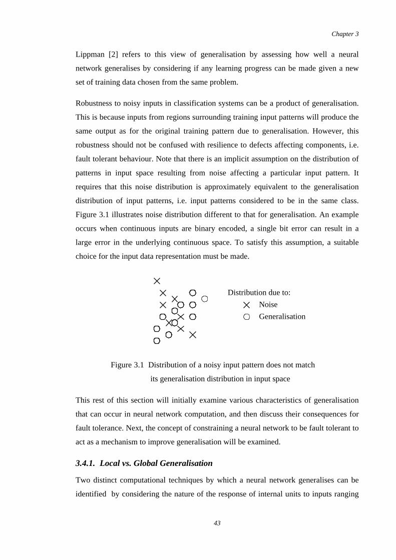
Lippman [2] refers to this view of generalisation by assessing how well a neural
network generalises by considering if any learning progress can be made given a new
set of training data chosen from the same problem.
Robustness to noisy inputs in classification systems can be a product of generalisation.
This is because inputs from regions surrounding training input patterns will produce the
same output as for the original training pattern due to generalisation. However, this
robustness should not be confused with resilience to defects affecting components, i.e.
fault tolerant behaviour. Note that there is an implicit assumption on the distribution of
patterns in input space resulting from noise affecting a particular input pattern. It
requires that this noise distribution is approximately equivalent to the generalisation
distribution of input patterns, i.e. input patterns considered to be in the same class.
Figure 3.1 illustrates noise distribution different to that for generalisation. An example
occurs when continuous inputs are binary encoded, a single bit error can result in a
large error in the underlying continuous space. To satisfy this assumption, a suitable
choice for the input data representation must be made.
This rest of this section will initially examine various characteristics of generalisation
that can occur in neural network computation, and then discuss their consequences for
fault tolerance. Next, the concept of constraining a neural network to be fault tolerant to
act as a mechanism to improve generalisation will be examined.
3.4.1. Local vs. Global Generalisation
Two distinct computational techniques by which a neural network generalises can be
identified by considering the nature of the response of internal units to inputs ranging
Noise
Generalisation
Distribution due to:
Figure 3.1 Distribution of a noisy input pattern does not match
its generalisation distribution in input space
Chapter 3
43
over the input space. Some neural networks employ units which only activate for inputs
in a limited bounded region of input space, e.g. Radial Basis Function networks [94]
and CMAC networks [86]. An unknown input will only activate those units whose
activation regions includes the new input. Other units will remain inactive. So, the
generation of a suitable output is only influenced by the units whose activation regions
surround the input pattern. Due to the limited region of input space involved in
generalising a new input, this form of generalisation is termed local.
The other computational method by which unknown inputs are processed is termed
global generalisation. This is where the internal units of a neural network respond to all
inputs lying anywhere within the input space. An example is the multi-layer perceptron
network [21] where the output of a unit is determined by a function of the distance of
its input from a hyperplane. An unknown input will cause all units to respond, and their
combined computation provides a suitable output.
Relationships can be drawn between these two facets of generalisation and the concept
of distribution in neural networks. Global generalisation implies that a more distributed
representation can be formed since the function of all units must be altered during
learning for every input pattern. However, locally generalising neural networks will
clearly favour local representations. Also, information processing will be more
distributed given global generalisation since all units are functionally active, as opposed
to only a few active units in the case of local generalisation.
These two computational techniques for generalisation result in different characteristics
for the possible fault tolerance of a neural network. If generalisation is local then it
implies that faults will cause generalisation to be suddenly unreliable in limited regions
of input space. Outside these local regions generalisation will be unaffected. This will
result in a system whose reliability is highly uncertain. Only when an input falls into a
region where the neural network's operation is affected will the effect of faults be
apparent and possible failure occur. However, faults affecting a neural network which
exhibits global generalisation will cause a small loss of generalisation for any input
pattern. This results in the effect of faults on the reliability of the neural network to be
more uniform across the input space, but less drastic.
Chapter 3
44
It is more difficult to compare the redundancy gained between globally and locally
generalising neural networks when their capacity is increased, for example, adding an
extra unit. Global generalisation implies that all units are involved in any computation,
and so increasing capacity will be observed across the whole system. However, for a
neural network which exhibits local generalisation, extra units will only increase
redundancy for patterns from a limited region of input space. This corresponds with the
above discussion on graceful degradation in locally and globally generalising neural
networks.
Overall, due to the combination of redundancy potentially increasing reliability
throughout a neural network and a more uniform effect of faults across the input space,
it would seem preferable to use a globally generalising neural network in a system. For
these reasons, only globally generalising neural networks will be examined in this
thesis.
However, it should be noted that if a large number of extra units are used in a locally
generalising neural network, the degree of overlap between the input space regions of
each unit can be increased such that a general improvement in fault tolerance will be
achieved. It is not obvious whether a similarly increased capacity in an equivalent
globally generalising neural network will be more effective.
3.4.2. Interpolation vs. Inexact Classification
As well as the various properties of generalisation due to the functional operation of a
neural network as described above, generalisation can also be differentiated depending
upon the nature of its application. The most common problem domains in which neural
networks have been employed are either to categorise input patterns into a set of
classes, or else to evaluate a functional mapping. The choice of thresholding function
employed in its output units is the principle influence determining which type of
operation a neural network performs. A pattern classification system uses non-linear or
hard-limited thresholded units to form discrete output patterns, while linear output units
are employed for functional mapping systems to produce continuous output values.
The style of generalisation required in both cases is very different. In the case of pattern
classification, inexact classification is required, while for functional evaluation,
interpolation is more suitable (see figure 3.2). These two areas will now be considered
Chapter 3
45
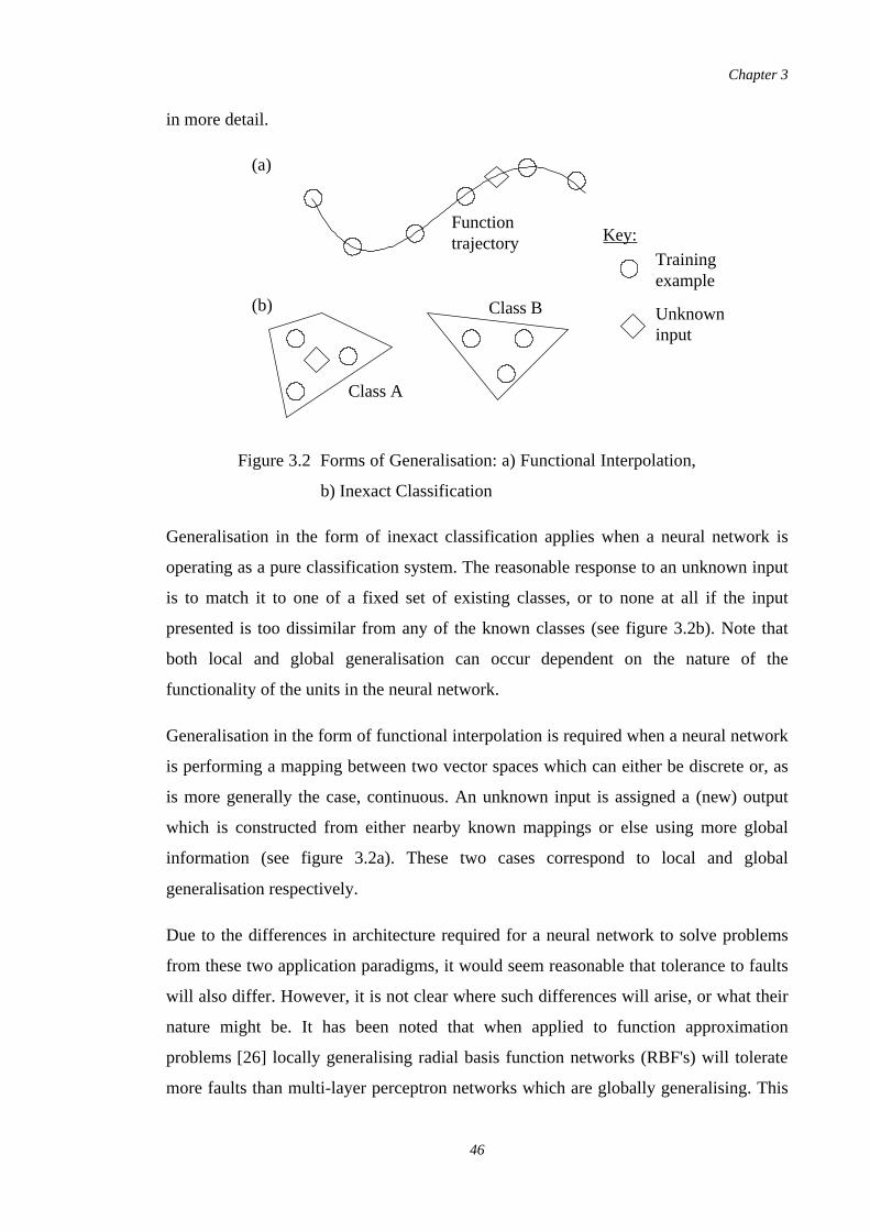
in more detail.
Generalisation in the form of inexact classification applies when a neural network is
operating as a pure classification system. The reasonable response to an unknown input
is to match it to one of a fixed set of existing classes, or to none at all if the input
presented is too dissimilar from any of the known classes (see figure 3.2b). Note that
both local and global generalisation can occur dependent on the nature of the
functionality of the units in the neural network.
Generalisation in the form of functional interpolation is required when a neural network
is performing a mapping between two vector spaces which can either be discrete or, as
is more generally the case, continuous. An unknown input is assigned a (new) output
which is constructed from either nearby known mappings or else using more global
information (see figure 3.2a). These two cases correspond to local and global
generalisation respectively.
Due to the differences in architecture required for a neural network to solve problems
from these two application paradigms, it would seem reasonable that tolerance to faults
will also differ. However, it is not clear where such differences will arise, or what their
nature might be. It has been noted that when applied to function approximation
problems [26] locally generalising radial basis function networks (RBF's) will tolerate
more faults than multi-layer perceptron networks which are globally generalising. This
(a)
(b)
Trainingexample
Unknowninput
Key:
Class A
Class B
Functiontrajectory
Figure 3.2 Forms of Generalisation: a) Functional Interpolation,
b) Inexact Classification
Chapter 3
46
is since the effect of faults is strictly limited within the problem space due to the local
nature of the operation of the units used in RBF's. For regions away from the fault, no
effect will occur. When an input is presented that lies within the region affected by the
fault(s) only if sufficient numbers of units in the locality exist will successful
functionality be possible. However, this seems rather wasteful in terms of resources and
implies that the holistic properties of distributed information storage will be weakened
due to the more local representation formed. For this reason globally generalising
neural networks are preferable. To achieve fault tolerance better training techniques are
required.
Note that the functional interpolation style of generalisation does not just apply to
neural networks performing a continuous function mapping (e.g. in robot control [95]),
it can also apply to classification problems where an interpolation to an unknown input
can also be appropriate. For example, if a neural network is trained to distinguish
different line segment orientations then it is useful if it can also recognise and give a
suitably interpolated output for line segments at orientations between those given as
examples during training. This occurs naturally in Kohonen networks [91].
3.4.3. Fault Tolerance as a Constraint
It has been proposed by various researchers that a requirement for fault tolerance can be
applied as a constraint in a neural network to achieve generalisation3 [28]. One study
has shown that this concept does have some empirical justification. A training method
which induces fault tolerance by injecting transient faults (described by Sequin and
Clay [71]) was shown to improve generalisation [96]. However the classification
problem used was extremely simple, but it is an indication that this concept bears
further investigation.
One of the questions which arises when training a neural network (section 3.2) is
deciding its size so that it will just be able to solve the problem. Too few units result in
the neural network unable to learn fully the problem. Conversely it has been commonly
found that if too many units are used in a neural network then its ability to generalise is
much diminished. This has been variously ascribed to overtraining, learning noise
within the training set, and memorising individual members of the training set rather
3 Personal communication, Dr. Bruce Segee, University of New Hampshire (August 1991).
Chapter 3
47
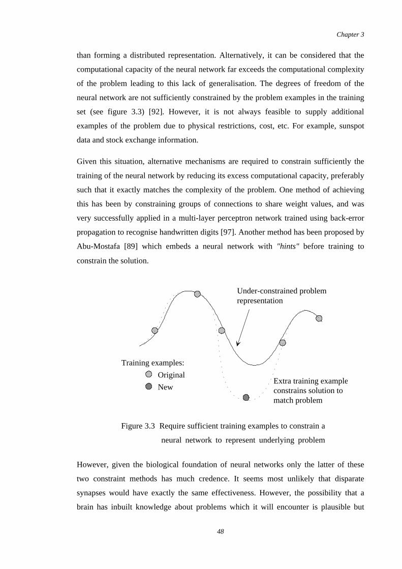
than forming a distributed representation. Alternatively, it can be considered that the
computational capacity of the neural network far exceeds the computational complexity
of the problem leading to this lack of generalisation. The degrees of freedom of the
neural network are not sufficiently constrained by the problem examples in the training
set (see figure 3.3) [92]. However, it is not always feasible to supply additional
examples of the problem due to physical restrictions, cost, etc. For example, sunspot
data and stock exchange information.
Given this situation, alternative mechanisms are required to constrain sufficiently the
training of the neural network by reducing its excess computational capacity, preferably
such that it exactly matches the complexity of the problem. One method of achieving
this has been by constraining groups of connections to share weight values, and was
very successfully applied in a multi-layer perceptron network trained using back-error
propagation to recognise handwritten digits [97]. Another method has been proposed by
Abu-Mostafa [89] which embeds a neural network with "hints" before training to
constrain the solution.
However, given the biological foundation of neural networks only the latter of these
two constraint methods has much credence. It seems most unlikely that disparate
synapses would have exactly the same effectiveness. However, the possibility that a
brain has inbuilt knowledge about problems which it will encounter is plausible but
Under-constrained problemrepresentation
Extra training exampleconstrains solution tomatch problem
Training examples:
Original
New
Figure 3.3 Require sufficient training examples to constrain a
neural network to represent underlying problem
Chapter 3
48
only at a very basic level, such as the initial structure of synaptic connections,
interconnections between various modules, etc. The amount of information which can
potentially be stored in the brain far exceeds that which can be represented in the genes.
So only very basic constraints would be plausible.
The alternative method of constraining learning in a neural network by imposing the
condition that it is fault tolerant, as mentioned above, will now be considered. To
achieve fault tolerance, a degree of redundancy in some form will have to be developed
in the neural network during training, and this will reduce its computational capacity as
required. In biological neural networks it is evident that they are extremely fault
tolerant. However, it will be seen that this is not an inherent feature in artificial neural
networks, and must be developed using suitable techniques during training. This
discrepancy is an indication that fault tolerance is perhaps a constraint employed by
nature to develop neural systems which can successfully generalise.
Another significant advantage of applying fault tolerance as a constraint is that it
provides a mechanism for a neural network to be scalable [98], i.e. it can increase or
decrease the complexity of the problem which it solves. This is since the degree of
redundancy evolved during initial training to produce fault tolerant operational
behaviour can be reduced if the complexity of the problem which the neural network
solves increases, or vice versa. This can be seen to occur in a limited manner in the
Hopfield model [13] where a tradeoff exists between the number of the patterns that can
be stored and the network's fault tolerance [32]. As more patterns are stored the
complexity of the problem is increased and the observed fault tolerance decreases.
3.5. Architectural Aspects of Neural Networks
It has already been noted that neural networks consist of many simple (often
homogeneous) processing elements connected via a complex communication network.
Typical neural networks which have been taught to solve problems such as reading text
[99] recognising sonar images [100], etc. have a few hundred units and many thousand
weighted connections. The combination of extreme simplicity in individual processing
units and the multitude of units and connections implies that the failure of a particular
computational element should not be critical for the operation of the system. This is
Chapter 3
49
often argued to imply that a degree of fault tolerance should exist in artificial neural
networks due to the existence of such redundancy.
In terms of information distribution each processing unit has a large fan-in of data on
which a relatively simple computation is performed. It seems likely, even if a
proportion of the incoming information is erroneous or nonexistent, that the unit should
still be able to function correctly in some limited fashion. Also, a processing unit feeds
many others and the information produced can be seen to be widely distributed in the
rest of the network. So even if some of its output communication paths are destroyed,
the information is not totally lost. It will be seen in chapter 6 that these two
architectural concepts do give rise to fault tolerance in multi-layer perceptron networks
as proposed here.
Some neural networks operate in an iterative manner, i.e. the final output is produced
by a repeated series of identical processing steps rather than just a single sequence of
operations being performed in one stage. An example is the Hopfield model [13]. At
each step the output converges towards the ultimate answer. This can be related to
temporal fault tolerance in the sense that small errors produced by faults at any stage
can be corrected by later steps in the processing due to their identical nature.
It can be seen that the peculiar architectural nature of neural networks tends to support
the reasoning that a degree of inherent fault tolerance should exist in artificial neural
networks. However, it will be seen that current training methods do not always produce
a neural network in which these fault tolerance inducing features are used to their
greatest extent.
3.6. Failure in Neural Networks
Failure in a system can be defined as the system not functioning as specified. This may
result in it producing erroneous results or not meeting performance goals such as timing
or consistency, etc. A more general definition, but weaker, would be that the system
does not meet the users' requirements. However, since the specification should define
precisely what these requirements are, the former definition of failure is more generally
accepted. In contrast, the user's definition of what the system should perform can
Chapter 3
50
change or even be inconsistent. Also, it is not easy to define formally and so recognise
failure for this case.
In a conventional computing system failure tends to be an abrupt halt of service.
However, neural networks naturally tend to exhibit graceful degradation (c.f. chapter
4), i.e. the service provided by the system deviates gradually from that specified. The
argument underlying this claim tends to rely on the distributed nature of neural
networks. However, it will be shown below that it is the computational style of neural
networks coupled with the nature of the problem domains for which neural networks
are best suited which gives rise to this graceful degradation.
Since this continuous manner of failure occurs naturally in neural networks it allows
systems to be developed which have very useful innate properties. For instance, in the
control of dynamic systems faults will not cause a catastrophic event, but rather the
precision of control will be degraded. An example is the truck-backer-upper system
developed by Widrow et al [101] which controls the direction of a reversing articulated
truck such that it eventually docks at a loading bay. When faults occur within the neural
network, the truck still reverses to the docking bay, but in a similar fashion to a "drunk"
driver4 (c.f. chapter 2). It should also be noted that special design techniques to achieve
graceful degradation which would normally have to be applied during the development
of a system using conventional computational structures will no longer be necessary
when using neural networks.
3.7. Problem Classification
Neural networks are particularly successful in learning to solve certain types of
problems such as image recognition, classification, controlling dynamic systems, etc.
These are termed soft problems. Similarly though, other (rigid) problems prove
incredibly difficult for a neural network to learn, e.g. digital arithmetic operations. In
general, a complex problem can be split into many sub-problems, and each will fall into
one of the two classes above.
It is no coincidence that the capabilities of neural networks in these two classes of
problems corresponds closely with those of biological neurocomputers, such as our own
4 Personal communication, Professor Widrow (July 1991)
Chapter 3
51
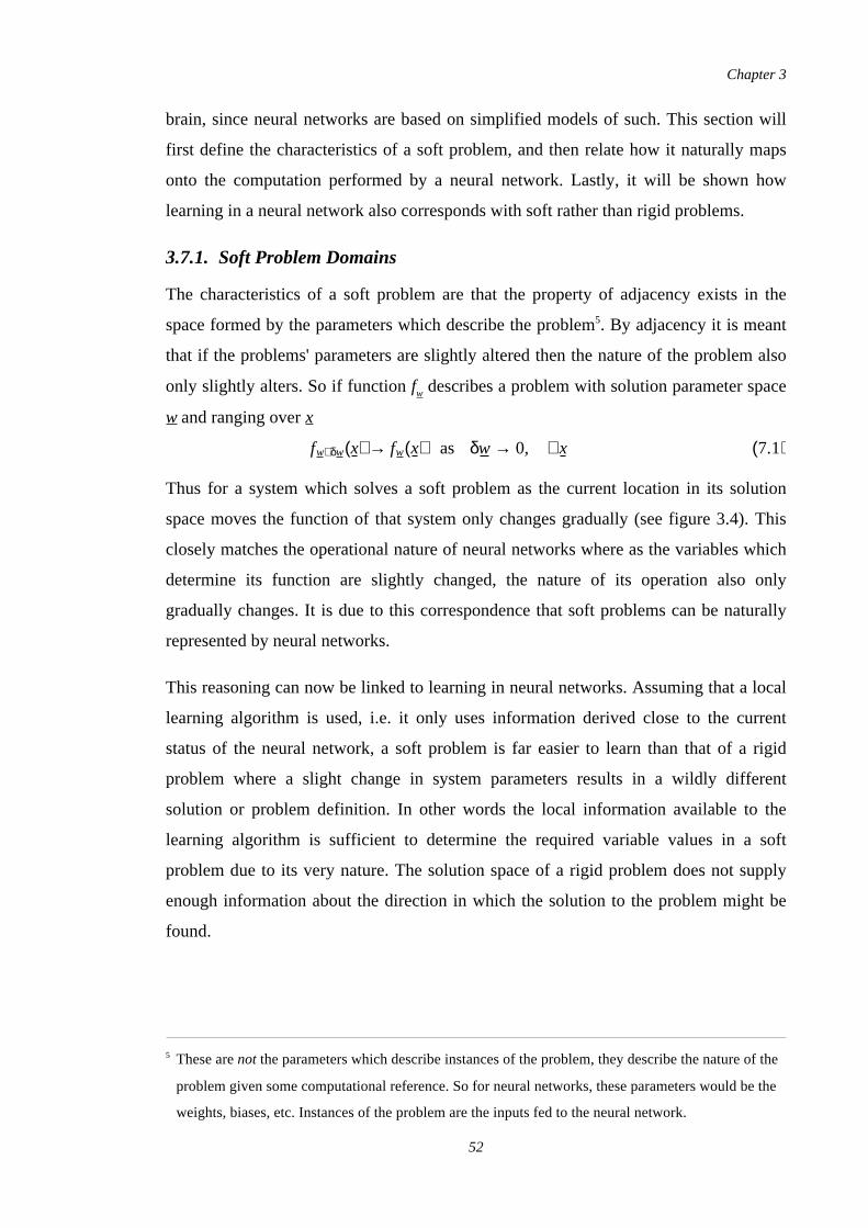
brain, since neural networks are based on simplified models of such. This section will
first define the characteristics of a soft problem, and then relate how it naturally maps
onto the computation performed by a neural network. Lastly, it will be shown how
learning in a neural network also corresponds with soft rather than rigid problems.
3.7.1. Soft Problem Domains
The characteristics of a soft problem are that the property of adjacency exists in the
space formed by the parameters which describe the problem5. By adjacency it is meant
that if the problems' parameters are slightly altered then the nature of the problem also
only slightly alters. So if function fw describes a problem with solution parameter space
w and ranging over x
Thus for a system which solves a soft problem as the current location in its solution
space moves the function of that system only changes gradually (see figure 3.4). This
closely matches the operational nature of neural networks where as the variables which
determine its function are slightly changed, the nature of its operation also only
gradually changes. It is due to this correspondence that soft problems can be naturally
represented by neural networks.
This reasoning can now be linked to learning in neural networks. Assuming that a local
learning algorithm is used, i.e. it only uses information derived close to the current
status of the neural network, a soft problem is far easier to learn than that of a rigid
problem where a slight change in system parameters results in a wildly different
solution or problem definition. In other words the local information available to the
learning algorithm is sufficient to determine the required variable values in a soft
problem due to its very nature. The solution space of a rigid problem does not supply
enough information about the direction in which the solution to the problem might be
found.
5 These are not the parameters which describe instances of the problem, they describe the nature of the
problem given some computational reference. So for neural networks, these parameters would be the
weights, biases, etc. Instances of the problem are the inputs fed to the neural network.
fw+δw(x) → fw(x) as δw → 0, ∀ x (7.1)
Chapter 3
52
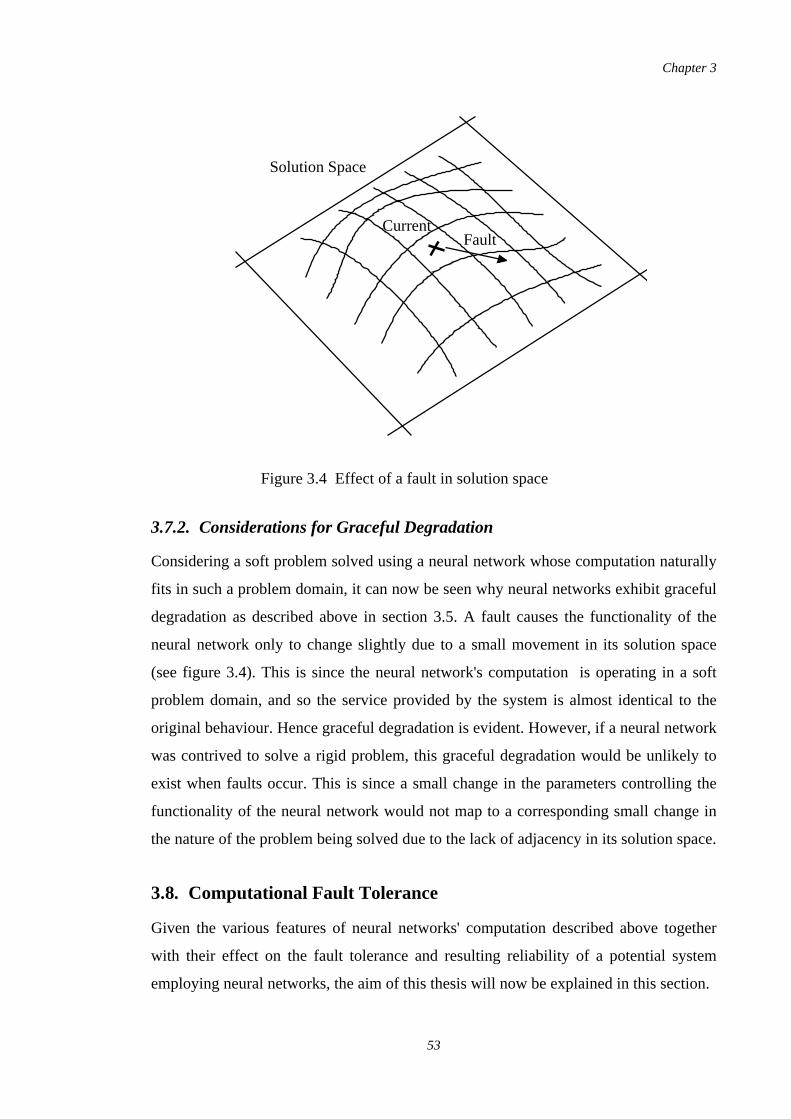
3.7.2. Considerations for Graceful Degradation
Considering a soft problem solved using a neural network whose computation naturally
fits in such a problem domain, it can now be seen why neural networks exhibit graceful
degradation as described above in section 3.5. A fault causes the functionality of the
neural network only to change slightly due to a small movement in its solution space
(see figure 3.4). This is since the neural network's computation is operating in a soft
problem domain, and so the service provided by the system is almost identical to the
original behaviour. Hence graceful degradation is evident. However, if a neural network
was contrived to solve a rigid problem, this graceful degradation would be unlikely to
exist when faults occur. This is since a small change in the parameters controlling the
functionality of the neural network would not map to a corresponding small change in
the nature of the problem being solved due to the lack of adjacency in its solution space.
3.8. Computational Fault Tolerance
Given the various features of neural networks' computation described above together
with their effect on the fault tolerance and resulting reliability of a potential system
employing neural networks, the aim of this thesis will now be explained in this section.
CurrentFault
Solution Space
Figure 3.4 Effect of a fault in solution space
Chapter 3
53
As already stated, the aim of this thesis is to examine the computational fault tolerance
of artificial neural networks rather than that arising from any implementation
technologies. More specifically, the operational fault tolerance rather than the learning
fault tolerance of neural networks is to be examined [19], i.e. the resistance of trained
neural networks to the effects of faults during actual operation rather than during their
learning phase.
The term computational fault tolerance refers to a system being resilient to changes in
its overall functionality arising from the operation of abstract components in the system
being defective. The methodology for both selecting these components from an abstract
system definition and the manner in which they are defective (i.e. constructing a fault
model) will be explained in chapter 4.
Computational fault tolerance is subtly different to the physical fault tolerance of an
implementation since it considers the effect of "faults" on a system at a much higher
level of abstraction. For physical fault tolerance the faults modelled are based on
physical defects which could occur in the system, though abstracted due to
computational necessity (see chapter 4). However, for computational fault tolerance it is
the system which is abstracted, and then faults are based on actual components in this
abstracted definition. This alternative technique for studying the fault tolerance of a
system allows the possible fault tolerance within a computational paradigm to be
analysed before any implementation level design questions have to be answered.
However, it is not viewed as supplanting studies of the fault tolerance of possible
implementations, but rather it is an approach to guide development decisions during
system design. Both methods supply information on the effect of faults in a system but
just at different levels of abstraction.
The reasons for choosing to study this abstract form of fault tolerance rather than that at
an implementation level are:
There currently exists a lack of a suitable implementation technology for
neural networks. Individual units have very simple computation which does
not need high-speed components, but a fast, complex (three dimensional) and
dense communication medium is required. Silicon technology is at a tangent
to this requirement since it provides the ability to develop fast processors but
Chapter 3
54

slow communications. Of more potential benefit is optical technology, but this
is still not fully developed.
It allows the commonly asserted statement that neural networks are inherently
fault tolerant due to their style of computation, distributed storage, etc. to be
examined. Also, the fault tolerance of neural networks can be studied free
from the influences arising from any particular fabrication technology
employed.
Will allow general results to be found on the fault tolerance of neural
networks that will provide information for many models and also supply
guide-lines for future implementations.
Analysis of the effect of specific features in neural network's computation as
described in this chapter on fault tolerance are possible.
Limit scope of this research.
Although only the computational fault tolerance of neural networks will be examined in
this thesis for the various reasons given above, the results should have relevance for
future implementation designs. By studying the resistance of the computational style of
neural networks to certain deformations, implementations will be able to take advantage
of such computational fault tolerance that inherently exists. However, note that it
clearly is also possible that conventional fault tolerant techniques could be applied in a
design such as N-Modular Redundancy [4], etc.
3.9. Verifying an Adaptive System
This area will not be examined in any depth in this dissertation, but it is useful to
discuss a few of the major aspects in the problem of verifying an adaptive system
considering the potential promise of neural networks.
In section 3.2, the process of learning in neural networks was discussed. Although this
capability has great potential benefits, it also gives rise to some complications. An
adaptive system is generally considered unacceptable for use in a situation where
reliability of operation is paramount. This is because it is unclear how to verify that the
learning process always produces a system with the required functionality. Also, in the
case of on-line adaptation, i.e. the function of a system changes during operational use
Chapter 3
55
it must be shown that the learning process causes the system's functionality always to
match more closely the required functionality. In the vast majority of neural network
applications to date teaching is only performed before operational use. The verification
of the trained neural network's operation is very difficult, though it is believed that
computational learning theory [93] may be a tool which would be useful in undertaking
this task.
3.10. Conclusions
This chapter has examined various concepts of neural network's computational nature
such as distribution of information, generalisation, graceful degradation, etc. Also, the
types of problems which neural networks are best suited to have been discussed, and the
influence these have on the potential reliability of a system employing neural networks
examined. The graceful degradation which is prevalent in neural networks has been
shown to arise from the soft problem domains in which neural networks are typically
applied coupled with the computational nature of neural networks lending itself to such
problem domains. Given these issues, the aim of this thesis in studying the
computational, rather than physical, fault tolerance of neural networks has been
explained and justified.
Chapter 3
56
CHAPTER FOUR
A Methodology for Fault Tolerance1
4.1. Introduction
To study the fault tolerance of artificial neural networks as proposed in this thesis, two
issues will first have to be examined. The first addresses the question of which
components in a neural network could become defective and also the nature of their
defect, i.e. defining a fault model. A useful property would be if the fault model could
be made generic across many neural network models.
The second issue concerns how a neural network's reliability should be assessed. The
methodology described in the following sections provides a base from which research
into the fault tolerance of a neural network can be performed.
Although in this thesis only the computational fault tolerance of a neural network is
studied (c.f. chapter 3), it is proposed that the techniques given below for defining a
fault model and assessing reliability are also suitable when examining the fault
tolerance of neural hardware.
Section 4.2 considers general notions about the construction of fault models. Various
levels of visualisation for neural networks are then described in section 4.3, and the
problems of considering neural networks at an abstract level are discussed. Section 4.4
examines the locations chosen for defects in various conventional fault models, and
from this, section 4.5 describes how locations for faults can be selected from an abstract
definition of a neural network. Section 4.6 then gives two rules that should be followed
in defining the nature of such faults. Various considerations pertaining to spatial and
temporal aspects of neural networks and their application are then considered with
regard to assessing fault tolerance in section 4.7. Finally, the construction of fault
1 Parts of this chapter have been published in IJCNN-91 Singapore [111,112].
Chapter 4
57
models for artificial neural networks is summarised in section 4.8. Section 4.9 briefly
considers the role of functional fault models. The concept of fault coverage is described
in section 4.10, and the degree of coverage in a fault models constructed using the
method described in this chapter is considered.
Section 4.11 discusses reliability in neural networks, and then section 4.12 considers
how to measure the degree of failure in a neural network. Section 4.13 relates this to
assessing how fault tolerant a neural network is. Finally, section 4.14 discusses various
simulation frameworks within which the fault tolerance of a neural network can be
assessed, especially so that comparative results can be obtained.
4.2. Fault Models
The development of fault models is an essential part of the process in determining the
reliability of a neural network system. A fault model describes the types of faults that a
system can develop, specifying where and how they will occur in it. However, faults
become more difficult to formulate sensibly as a system is viewed at an increasingly
more abstract level, especially the definition of how a fault manifests itself. It will be
shown below how sensible locations for faults can be defined in a neural network
viewed at the abstract level, and then the complex problem of how to detail the effect of
faults in these locations will be approached.
The entities listed in a fault model need not necessarily physically exist, but may be
abstractions of real-world objects. In general, a fault model is an abstracted
representation of the physical defects which can occur in a system, such that it can be
employed to usefully, and reasonably accurately, simulate the behaviour of the system
over its intended lifetime with respect to its reliability. Four major goals exist when
devising a fault model:
1. The abstract faults described in the model should adequately cover the
effects of the physical faults which occur in the real-world system.
2. The computational requirements for simulation should be satisfiable.
3. The fault model should be conceptually simple and easy to use.
4. It should provide an insight into introducing fault tolerance in a design.
Chapter 4
58
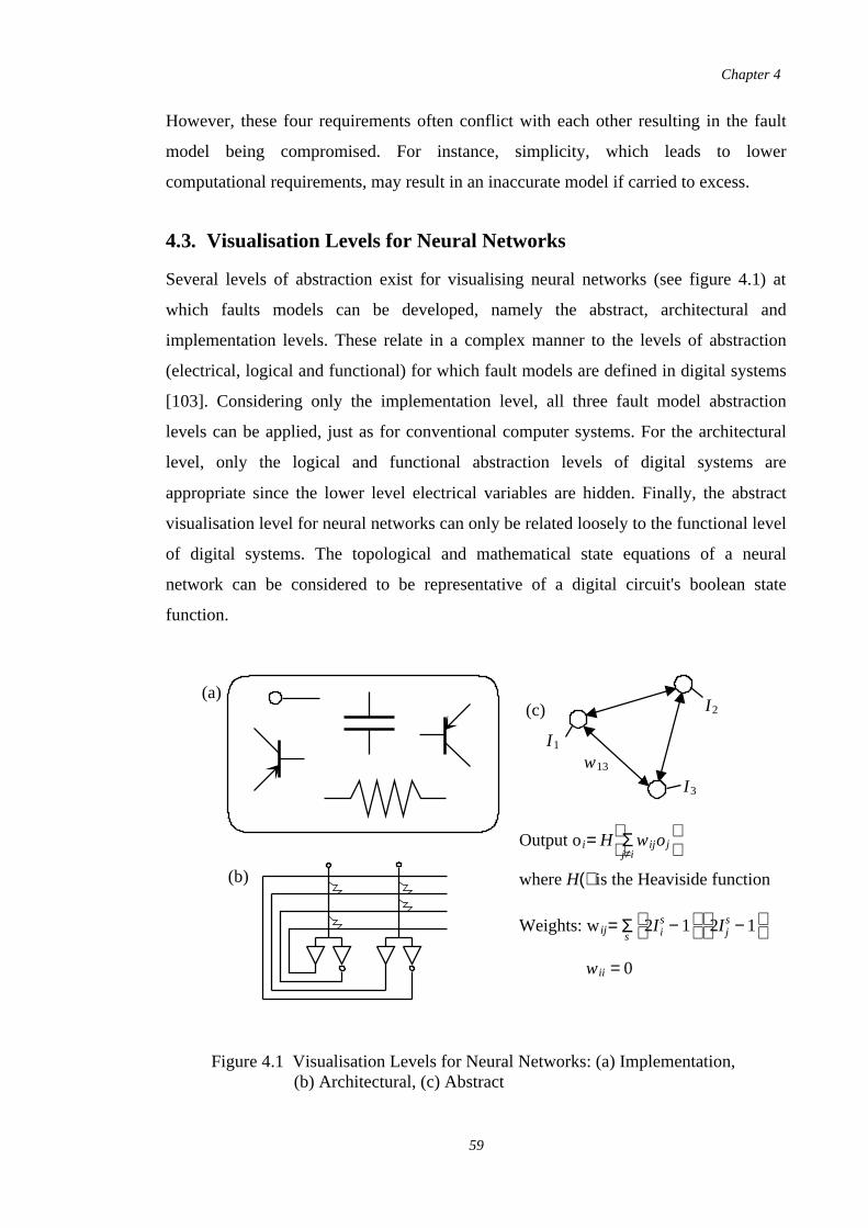
However, these four requirements often conflict with each other resulting in the fault
model being compromised. For instance, simplicity, which leads to lower
computational requirements, may result in an inaccurate model if carried to excess.
4.3. Visualisation Levels for Neural Networks
Several levels of abstraction exist for visualising neural networks (see figure 4.1) at
which faults models can be developed, namely the abstract, architectural and
implementation levels. These relate in a complex manner to the levels of abstraction
(electrical, logical and functional) for which fault models are defined in digital systems
[103]. Considering only the implementation level, all three fault model abstraction
levels can be applied, just as for conventional computer systems. For the architectural
level, only the logical and functional abstraction levels of digital systems are
appropriate since the lower level electrical variables are hidden. Finally, the abstract
visualisation level for neural networks can only be related loosely to the functional level
of digital systems. The topological and mathematical state equations of a neural
network can be considered to be representative of a digital circuit's boolean state
function.
Chapter 4
59
(a)
(b)
(c)
w13
Output oi= H Σ
j≠iwij oj
where H() is the Heaviside function
Weights: w ij = Σs
2I i
s − 1
2I j
s −1
wii = 0
I 1
I 3
I 2
Figure 4.1 Visualisation Levels for Neural Networks: (a) Implementation,(b) Architectural, (c) Abstract
In general, just as for the levels of abstraction for viewing digital systems, it becomes
progressively harder to define good fault models as one moves from the implementation
level to the abstract level for neural networks. For example, in digital systems it is
impossible to model current leakage at the logical level, but it can be modelled at the
lower electrical level. Restrictions also arise due to the simplification of continuous
electrical parameters to logical values.
4.3.1. Abstract Level
The objective in this thesis is to investigate the inherent fault tolerance of neural
networks which arises from their unusual computational features, such as distribution of
information, generalisation, etc. It is not to directly examine the characteristics of
physical implementations, either at the architectural or implementational level, where
reliability will be influenced by the physical components and fabrication techniques
employed. This means that employing concepts from the electrical and architectural
levels will not be appropriate. The main reason for taking this approach is that
implementation and architectural levels are too specific; technologies change and
architectures are numerous. This investigative direction will allow implementations of
neural networks to be designed in such a way so as to retain the inherent fault tolerance
within the model, as well as to enhance it by means of standard fault tolerance design
procedures.
Examining neural networks at the abstract level suggests that the definition of a fault
model is likely to be difficult, and also at first view, there seems to be a conflict with
the requirement that a fault model should adequately cover real-world defects.
However, although it is possible to identify reasonably the potential faulty entities in the
abstract model of the neural network, it will be seen that reference occasionally must be
made to implementation aspects of possible designs when describing the nature of their
deviation from proper behaviour. This leads to acceptable fault coverage. Also, viewing
a neural network at an abstract level implies that the further goal in the development of
a fault model of disassociating it from any particular class of neural network will be
eased. This will allow comparisons between results from such neural models, thus
indicating their relative merits.
Chapter 4
60
4.3.2. Role of Fault Models
The fault model once defined can be used for two purposes. Firstly, if it covers physical
faults satisfactorily, then it can be used in the generation and application of a test
procedure to ensure that an implemented system operates according to specification.
Secondly, the fault model can be used in simulations of the neural network system to
evaluate a measure for its reliability. It is this latter case which is of interest here. Two
approaches exist for developing a measure for reliability in a neural network system.
The first is to use measures from existing reliability theory and apply them to neural
network systems, the other is to develop new measures. Both of these avenues will be
explored further in section 4.9. The overall objective is to define measures which are
generic in nature; they should apply across a wide range of neural network architectures
such that valid comparisons can be made between them, and again, as for the fault
models, simplicity and ease of use should be major considerations.
4.4. Conventional Fault Models
In formulating the locations for faults in an abstract visualisation of a neural network, it
is helpful to first examine existing fault models for conventional digital systems.
Considering a system at its most basic level, the physical faults which occur depend
upon the fabrication techniques used to implement the circuit, such as TTL or CMOS
for example. A few examples of such physical faults for the latter technology are
defects in the silicon, short circuits in metal, and holes in oxides used in transistors.
These very real faults are modelled by some more abstract representation in the related
fault model such that both accuracy and simplicity are hopefully achieved. Three levels
of abstraction tend to be considered for viewing systems, each with its own associated
class of fault model. See figure 4.2 for an example of a component represented in
electrical, logical, and functional form.
At the very detailed electrical level, example definitions of faults are changes in various
continuous variables such as voltage, resistance, and current levels. However, such a
fault model can only be useful for very small and simple systems. The computational
cost of modelling these very detailed variables quickly becomes prohibitive.
Next, the logical level only considers signal values which map to the logic (and
discrete) 0 and 1 values, and the corresponding faults are similarly more abstract. The
Chapter 4
61
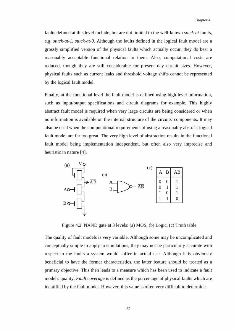
faults defined at this level include, but are not limited to the well-known stuck-at faults,
e.g. stuck-at-1, stuck-at-0. Although the faults defined in the logical fault model are a
grossly simplified version of the physical faults which actually occur, they do bear a
reasonably acceptable functional relation to them. Also, computational costs are
reduced, though they are still considerable for present day circuit sizes. However,
physical faults such as current leaks and threshold voltage shifts cannot be represented
by the logical fault model.
Finally, at the functional level the fault model is defined using high-level information,
such as input/output specifications and circuit diagrams for example. This highly
abstract fault model is required when very large circuits are being considered or when
no information is available on the internal structure of the circuits' components. It may
also be used when the computational requirements of using a reasonably abstract logical
fault model are far too great. The very high level of abstraction results in the functional
fault model being implementation independent, but often also very imprecise and
heuristic in nature [4].
The quality of fault models is very variable. Although some may be uncomplicated and
conceptually simple to apply in simulations, they may not be particularly accurate with
respect to the faults a system would suffer in actual use. Although it is obviously
beneficial to have the former characteristics, the latter feature should be treated as a
primary objective. This then leads to a measure which has been used to indicate a fault
model's quality. Fault coverage is defined as the percentage of physical faults which are
identified by the fault model. However, this value is often very difficult to determine.
A
B AB
(a)
(b) A B AB
0 0 10 1 11 0 11 1 0
V
A
B
A B
(c)
Figure 4.2 NAND gate at 3 levels: (a) MOS, (b) Logic, (c) Truth table
Chapter 4
62
4.5. Fault Locations
As each level (electrical, logical, functional) in a digital system requires a
corresponding fault model, the case is similar when considering fault models for neural
networks. When they are viewed from the implementation level, the conventional fault
models above can be employed, and for the higher architectural viewpoint, a functional
fault model is suitable. However, fault models for the implementation and architectural
levels cannot be specified generically since they are highly dependent upon the design
(e.g. the fabrication technology used), although standard existing fault models for
individual components (e.g. diodes, transistors, shift registers, etc.) could be envisaged
as building blocks in developing such a fault model. However, the objective here is that
of formulating a fault model for a neural network visualised from the abstract level. As
a further goal, the fault model should apply across a wide range of neural network
models. It is possible that functional fault models could be used since are independent
of system implementation, though they may be limited since the abstract description of
a neural network differs widely from model to model. Functional fault models applied
directly to neural networks will be discussed later in section 4.8.
Although not an objective of this thesis, examining the application of more
conventional fault models to neural networks viewed at the implementation and
architectural levels (c.f. section 4.3) illustrates how locations for faults in an abstractly
defined neural network can be found. By noting the common features, and then
extrapolating from these observations, it will be shown how new fault models can be
devised for the abstract visualisation level.
At the implementation level the electrical fault model involves physical objects such as
connection wires, capacitors, and transistors. The logical fault model refers to the
slightly more abstract signal lines which interconnect logic gates, and it is these entities
which are chosen to be possibly faulty. For example s-a-0, s-a-1, short-circuited, etc.
Next, at the higher architectural level, components such as individual IC's or
communication lines are chosen to be candidates for fault locations.
In both of these cases it can be seen that locations considered eligible for faults are
atomic entities with respect to the conceptual level at which the system is being viewed,
Chapter 4
63
or the tight interaction of a few such atomic entities. Also, these entities can be seen to
be either acting as functional units or information channels.
4.5.1. Fault Locations for Neural Networks
The above observation that the chosen elements which are selected to construct the fault
model at these two conceptual levels cannot be subdivided suggests that similarly at the
abstract level, the entities selected from the mathematical model should also not be
capable of being fragmented in terms of their role. For example, weights, links, and
threshold functions could all be candidates. Note that in addition, the entities from the
abstract definition which are eligible as fault locations should also have some
operational function or substance, rather than just being a temporary variable which is
used to connect various equations in the abstract definition together. For example,
output values associated with units are not considered eligible. A fault may cause an
output value to be erroneous, but faults cannot directly affect an output value.
In summary, to identify the various entities in a neural network, viewed at an abstract
level, which should be considered as being eligible for possible inclusion in a fault
model are any non-trivial atomic entities in the abstract definition of the neural
network. These entities should be limited to those which have potential for changing
information within the neural network, rather than those which merely transfer
information. Note that the generally large number of possible candidates for fault
locations arising from this procedure will be reduced when defining the manifestations
of the faults (section 4.6) and considering other factors (section 4.7).
Faults should be considered for both the operational and training phases of a neural
network, though only the former is vital when operational systems are going to be
"cloned" from a single once-only trained neural network. However, note that this is not
the case for an autonomous system employing neural networks since learning will be an
active function throughout its lifetime. Due to this, the abstract definition of a neural
network should also describe the learning algorithm.
This methodology provides a basis for a fault model which is independent of any
possible implementation, and simulation results should indicate the fault tolerance
inherent within the neural network model, i.e. that which arises as a consequence of the
nature of the computational method of neural networks.
Chapter 4
64
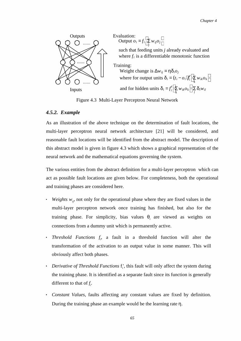
4.5.2. Example
As an illustration of the above technique on the determination of fault locations, the
multi-layer perceptron neural network architecture [21] will be considered, and
reasonable fault locations will be identified from the abstract model. The description of
this abstract model is given in figure 4.3 which shows a graphical representation of the
neural network and the mathematical equations governing the system.
The various entities from the abstract definition for a multi-layer perceptron which can
act as possible fault locations are given below. For completeness, both the operational
and training phases are considered here.
Weights wij, not only for the operational phase where they are fixed values in the
multi-layer perceptron network once training has finished, but also for the
training phase. For simplicity, bias values θi are viewed as weights on
connections from a dummy unit which is permanently active.
Threshold Functions fi, a fault in a threshold function will alter the
transformation of the activation to an output value in some manner. This will
obviously affect both phases.
Derivative of Threshold Functions f i', this fault will only affect the system during
the training phase. It is identified as a separate fault since its function is generally
different to that of fi.
Constant Values, faults affecting any constant values are fixed by definition.
During the training phase an example would be the learning rate η.
Chapter 4
65
Outputs
Inputs
......
......
......
Output oi = f i Σj wij oj
such that feeding units j already evaluated andwhere f i is a differentiable monotonic function
Weight change is ∆wij = ηδioj
where for output units δi = (t i − oi)f i Σk wikok
and for hidden units δi = f i Σk wikok
Σ
lδlwil
Figure 4.3 Multi-Layer Perceptron Neural Network
Evaluation:
Training:
Target Values ti, these are not included in the constant values above since it is
conceivable that a MLP network may be trained on data that is modified as time
progresses (e.g. Miikkulainen and Dyer [52]).
Topology, the connectivity of the neural network could easily be subject to faults
in various ways such as the loss of a connection between two units.
There also exist some entities which although they represent information, their lifetime
is strictly limited. For example, delta values δi have to be kept at each backward pass so
that errors can be evaluated at hidden units. However, they must be considered for
inclusion in the fault model due to their functional role in the operation of the
multi-layer perceptron network.
Activation Values .ai = Σj
wij oj
Delta δi, faults in these are only relevant during the training phase.
Weight Change ∆wij, these are the alteration for the stable weight base value, and
similarly as for δi, faults are only applicable during the training phase.
Note that the concept of a "unit" becoming faulty is not specified above, it is only a
further abstraction from fault locations such as the threshold function, activation values
ai, input weights wij, etc. This is analogous to a stuck-at fault in a digital circuit covering
many (more concrete) physical faults.
It can be seen that a large number of possible fault locations exist for a multi-layer
perceptron network. However, when the actual manifestations for these faults are
defined, it will be found that a large proportion of them can be discarded.
4.6. Fault Manifestations
Although the entities acting as possible locations for faults have been identified at the
abstract level from the mathematical model of a neural network, the actual nature of the
faults they suffer have yet to be defined. For instance, a threshold function might be
said to saturate (i.e. output one of its extreme values), a link in the topology might be
lost, a weight might be distorted in some way, etc. The latter example is especially
difficult to define sensibly since it is uncertain as to what form of distortion might
Chapter 4
66
reasonably occur in the abstract universe which is considered here. It is due to the
abstract conceptual level at which the fault tolerance of artificial neural network models
are being viewed that this difficulty arises.
It is proposed that two main concepts exist for defining the manifestation of faults. The
first is to look solely at the abstract description of the neural network, and from this
distortions in the abstract universe can be applied. The alternative is by relating fault
locations to high-level implementation details or physical components. The details of
the fault can then be extracted from these comparisons and any constraints that arise.
The use of the first guiding principle above can be approached by defining the
manifestation(s) of a fault to be such that the maximum harm is caused to the system's
operation by the fault. This will capture all possible lesser manifestations, whether
likely or unlikely. The notion of maximum harm will depend specifically on the
component's context for which the fault is to be defined. In some cases, several
manifestations may suggest themselves, for instance, due to symmetry such as in the
sigmoid thresholding function. Generally, the fault manifestation will be dynamic rather
than causing a static change to normal function, and can be viewed as being an active
fault mode. This is since it is unlikely that a static fault mode will cause maximum
damage in all possible operational states of an entity.
The alternative concept of considering the faults which could occur given certain
implementational restrictions will have the consequence of degrading the generality of
the fault model. This is since various design questions will have to be answered in
applying these restrictions, such as the fabrication technology to be used, storage
method of weights, etc. Since different neural network models may well lead to
different answers to these questions, possible generality in the fault model will be lost.
However, in certain cases it may be possible to minimise this by developing fault
models whose construction only relies on an abstracted view of possible
implementations.
The technique for defining fault manifestations used in this thesis is a combination of
the two directions described above. First, possible faults are defined using the
maximisation of damage principle. However, this tends to lead to extreme fault modes
being developed. The second direction using information derived from implementation
Chapter 4
67
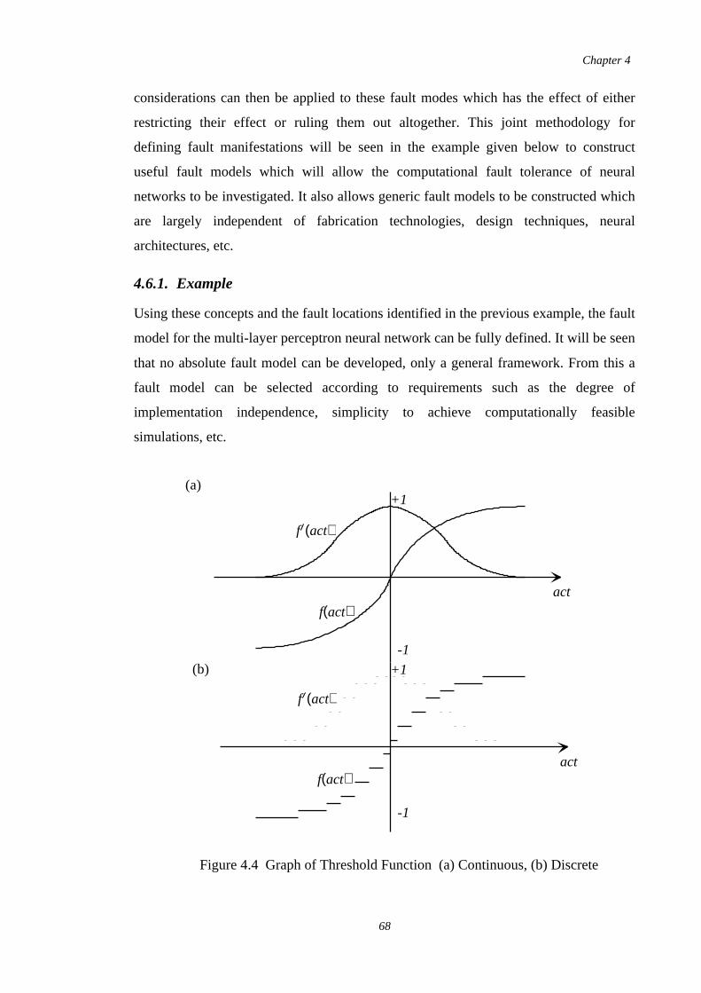
considerations can then be applied to these fault modes which has the effect of either
restricting their effect or ruling them out altogether. This joint methodology for
defining fault manifestations will be seen in the example given below to construct
useful fault models which will allow the computational fault tolerance of neural
networks to be investigated. It also allows generic fault models to be constructed which
are largely independent of fabrication technologies, design techniques, neural
architectures, etc.
4.6.1. Example
Using these concepts and the fault locations identified in the previous example, the fault
model for the multi-layer perceptron neural network can be fully defined. It will be seen
that no absolute fault model can be developed, only a general framework. From this a
fault model can be selected according to requirements such as the degree of
implementation independence, simplicity to achieve computationally feasible
simulations, etc.
Chapter 4
68
(b)
(a)
act
act
+1
-1
-1
+1
f (act)
f(act)
f(act)
f (act)
Figure 4.4 Graph of Threshold Function (a) Continuous, (b) Discrete
4.6.2. Threshold Function
The failure modes of the threshold function f, when considered only from the abstract
viewpoint, can best be defined by examining its graph (see figure 4.4a). The clear
symmetries in the threshold function suggests three possible failure modes. The first
two relate to the well-known stuck-at faults, and are defined here to be
stuck-at-minus-one and stuck-at-plus-one. However, this method of constructing a fault
model is not conducive for assessing the quality of fault coverage.
The alternative technique by applying the maximisation of damage principle suggests
another failure mode, and this is dynamic, rather than the static stuck-at faults. The
threshold function is defined to saturate to +1 when the fault-free output would be less
than zero, else -1 otherwise. This is a rather harsh fault during operational use2, since it
implies that the associated unit always outputs the incorrect value irrespective of "how
sure" it is, i.e. how large its activation is, and hence how close its fault-free output
would be to ±1. It could possibly be modified to take account of this by making the
fault probabilistic based on some function of the activation. For example,
. This shows how the two concepts for defining faultPr (Fault) = 1− f(act)
manifestations discussed previously can be jointly applied to develop a reasonable but
still wide-ranging fault mode.
The faults considered so far only apply to a continuous or analogue system. It is also
possible to define failure modes for a digital form of the threshold function (see figure
4.4b), though of course, this implicitly introduces reliance by the fault model on
implementation details. Example failure modes include elements of the digitised
function being corrupted, either randomly, or, by following the concept of maximum
damage, set to the opposite extreme of their fault-free value. This latter fault may again
be tempered by applying a similar probabilistic fault mode as above.
4.6.3. Differential of Threshold Function
The failure modes associated with the differential of the threshold function f' are similar
to the above. Since the graph peaks at +1 when act=0, and is symmetric about this
2 Note that during training, although more time will be required to teach a neural network if a unit
permanently reverses its threshold function, it is still very likely that the neural network will be able
to learn the training set to the same degree if no such fault had occurred.
Chapter 4
69

point (see figure 4.4), the two stuck-at faults should be stuck-at-plus-one and
stuck-at-zero.
To maximise the damage caused to the multi-layer perceptron's learning, the output
should be set to +1 as the fault-free value tends to 0, otherwise it should be set to 0. The
point of change could be defined to be where the sign of the curvature alters. This
causes the applied weight change to be always in the wrong direction. Similar failure
modes could be introduced for a discrete version of the function as described above.
4.6.4. Weights
Faults which affect the weights wij in a neural network are very hard to define sensibly
at an abstract level, though it will be seen that by using the maximisation of damage
principle this can be achieved. However, the first direction which applies "vague"
implementation information will be examined first. Two possibilities can be identified.
The weights can be considered as being held in a discrete form, such as binary
encoding, and then individual components can be corrupted in a similar fashion to that
for the discrete threshold function. The other alternative would be storing weights using
a continuous representation such as resistors for example. The model of the fault can
then be based on the fault characteristics of the component(s) used. For example, a
resistor is likely to either go open-circuit which can be modelled by causing the weight
to saturate to its maximum value, else it will become noisy which can be modelled by
adding noise from a Gaussian distribution.
However, the interest in this thesis is defining purely abstract failure modes for weights,
and as such, they will be independent of any implementation, and so the computational
fault tolerance of neural networks can be investigated. Two very simple failure modes
would be to either set the weight to zero, thus causing the loss of any partial
information (due to the distributed nature of neural network processing) that the weight
held. The other fault mode, following the concept of maximising damage, suggests that
the weight should be multiplied by -1. This represents a unit always trying to
misclassify an input.
Chapter 4
70
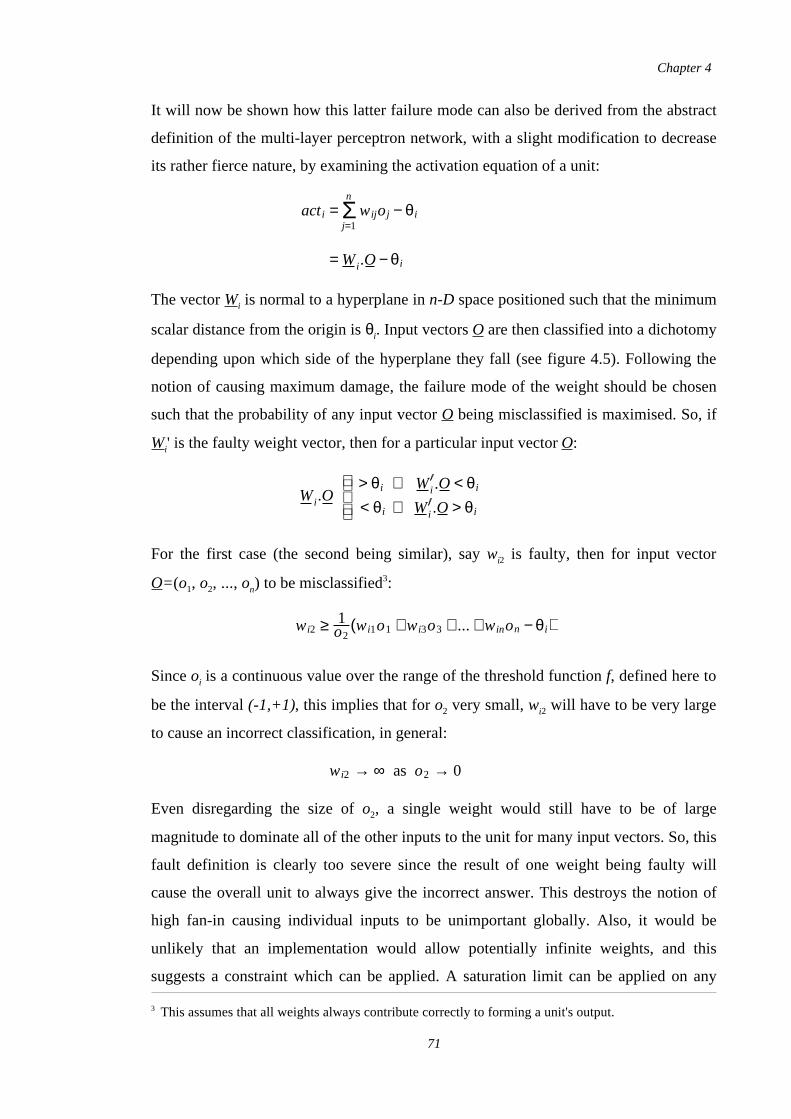
It will now be shown how this latter failure mode can also be derived from the abstract
definition of the multi-layer perceptron network, with a slight modification to decrease
its rather fierce nature, by examining the activation equation of a unit:
The vector Wi is normal to a hyperplane in n-D space positioned such that the minimum
scalar distance from the origin is θi. Input vectors O are then classified into a dichotomy
depending upon which side of the hyperplane they fall (see figure 4.5). Following the
notion of causing maximum damage, the failure mode of the weight should be chosen
such that the probability of any input vector O being misclassified is maximised. So, if
Wi' is the faulty weight vector, then for a particular input vector O:
For the first case (the second being similar), say wi2 is faulty, then for input vector
O=(o1, o2, ..., on) to be misclassified3:
Since oi is a continuous value over the range of the threshold function f, defined here to
be the interval (-1,+1), this implies that for o2 very small, wi2 will have to be very large
to cause an incorrect classification, in general:
Even disregarding the size of o2, a single weight would still have to be of large
magnitude to dominate all of the other inputs to the unit for many input vectors. So, this
fault definition is clearly too severe since the result of one weight being faulty will
cause the overall unit to always give the incorrect answer. This destroys the notion of
high fan-in causing individual inputs to be unimportant globally. Also, it would be
unlikely that an implementation would allow potentially infinite weights, and this
suggests a constraint which can be applied. A saturation limit can be applied on any
3 This assumes that all weights always contribute correctly to forming a unit's output.
act i = Σj=1
n
wij oj − θi
= Wi .O −θi
Wi .O
> θi ⇒ Wi .O < θi
< θi ⇒ Wi .O > θi
wi2 ≥ 1o2
(wi1o1 +wi3o3 + ...+winon −θi)
wi2 → ∞ as o2 → 0
Chapter 4
71
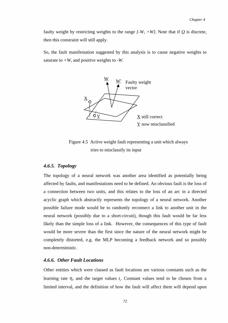
faulty weight by restricting weights to the range [-W, +W]. Note that if O is discrete,
then this constraint will still apply.
So, the fault manifestation suggested by this analysis is to cause negative weights to
saturate to +W, and positive weights to -W.
4.6.5. Topology
The topology of a neural network was another area identified as potentially being
affected by faults, and manifestations need to be defined. An obvious fault is the loss of
a connection between two units, and this relates to the loss of an arc in a directed
acyclic graph which abstractly represents the topology of a neural network. Another
possible failure mode would be to randomly reconnect a link to another unit in the
neural network (possibly due to a short-circuit), though this fault would be far less
likely than the simple loss of a link. However, the consequences of this type of fault
would be more severe than the first since the nature of the neural network might be
completely distorted, e.g. the MLP becoming a feedback network and so possibly
non-deterministic.
4.6.6. Other Fault Locations
Other entities which were classed as fault locations are various constants such as the
learning rate η, and the target values ti. Constant values tend to be chosen from a
limited interval, and the definition of how the fault will affect them will depend upon
W W' Faulty weightvector
X
Y still correct
now misclassified
X
Y
Figure 4.5 Active weight fault representing a unit which always
tries to misclassify its input
Chapter 4
72
their function in the case of trying to cause maximum damage. For the learning rate η,
extreme failure modes would be to set it to zero or to its highest possible value. Its
value will typically be in the range (0,1]. A fault affecting a target value ti could be that
its value is changed to be opposite to that in a fault-free situation, thus maximising
damage to the neural network's learning. Target values generally only take the two
values at the extreme ends of the threshold function range. As a less severe fault,
randomisation either supplying an offset or a new absolute value might be more suitable
in both cases. Considering general implementation details, constants or target values
might be encoded in binary form or produced by dedicated hardware, and so similar
failure modes could be used as described above for the weights.
Other entities which were identified in the MLP network as possible fault locations hold
information whose lifetime is strictly limited. These are the activation values ai, delta
values δi, and weight changes ∆wij . The activation values are required throughout both
the evaluation and training stages, though delta values are required only in the latter
stage, but all will need to be temporarily stored. To cause maximum damage, their
respective failure modes would be either to limit them to their opposite value, possibly
constraining the activation and delta values to some limited range, else to apply some
randomisation process to them in a similar manner to that for the weights (see above).
Weight changes need only be considered if they are required to be temporarily stored,
such as when momentum is used during training, and then their failure modes will be
similar to those already given.
4.7. Spatial and Temporal Considerations
The fault model can be simplified by considering the relative merits of each fault in the
system. If a fault only occurs in relatively few places whilst another is widespread, then
so long as the former does not occur with very large probability with relation to the
latter, it would be acceptable to disregard it. However, if a fault which occurs with low
probability has catastrophic effects, then it should be included. For example, in a RAM
chip the amount of circuitry for the actual storage of bits far outweighs that for
addressing, so when simulating the chip to examine its reliability, the addressing
circuitry is considered to be fault-free. Since in a large neural network the number of
weighted connections is likely to be far larger than the number of unit associated
Chapter 4
73
entities (e.g. threshold functions), then it would be reasonable that these could be
ignored during investigations.
Faults can be classified by two temporal characteristics, they are either permanent or
transient in nature. The most frequently occurring case has been found to be the latter
[104], and it can be further subdivided into "transient" and "intermittent" categories.
Transient faults are non-recurring, but intermittent faults occur given a set of
internal/external conditions, i.e. recurring. This latter form of temporary fault can
become permanent.
Due to the observed relative domination of transient faults [104], it is suggested that
any simulations or theory developed for neural network models should be based on only
transient faults occurring, though this will only become especially relevant for feedback
neural networks. This restriction is since any fault tolerance analysis will then produce
realistic data as to the behaviour of an implemented system. Also, it allows the
complexity of any potential fault model to be greatly, but reasonably, decreased.
The effect a fault has on a system will also depend upon when it actually occurs with
respect to the system's operation. For example, a fault affecting a weight which occurs
sometime between the forward and backward passes of the back-propagation algorithm
for multi-layer perceptron neural networks will have different consequences if it
happened to occur at the start of the forward pass. However, modelling this in the fault
model would greatly increase the complexity of any fault tolerance analysis. For this
reason it would be sensible to assume that the manifestation of a fault only occurs when
a functional sub-system of a neural network is not processing an input. This is a
reasonable assumption to make if the time taken for such a functional sub-system to
process its input is much less than the frequency at which inputs are presented.
4.8. Summary
In section 4.5 it was shown how locations for faults could be identified from an abstract
definition of a neural network. The manifestation of these faults was then considered in
section 4.6. Together with section 4.7, a selection of the possible fault modes can then
Chapter 4
74
be taken to compose the fault model. To summarise, the methodology for producing
such a fault model is as follows:
1. The atomic entities within the system viewed at the conceptual level at
which its fault tolerance is being examined must be extracted.
2. Discard from these entities any which would not have a significant effect on
the reliability of the system. This may be due to the number of such entities
in the overall system being very small as compared to other entities selected
in step 1.
3. For each entity, the manifestation of the faults affecting it can be defined by
applying the principle of causing maximum damage to the system's
computation, restricted by considering certain implementation details.
4.9. Functional Fault Models
The role of functional fault models for neural networks will now be examined. A
functional fault model for conventional digital systems offers independence from
implementation details, though often at the expense of exactness and completeness. For
combinatorial circuits, the faults can be described by modifications to the truth table,
and similarly the state transition table for sequential circuits. When considering higher
level components (e.g. RAMs) as the atomic entities of the circuit, more complex
descriptions than truth or state transition tables need to be employed, and generally,
some formal descriptive language, embedding boolean expressions, is used [103].
However, since the majority of neural networks are of a continuous nature (rather than
the logical 1 and 0 of digital circuits), such methods are not applicable. For Boolean
neural networks [105] though, they can be directly applied since each unit can be
viewed as performing a fixed boolean expression which can be described by a truth
table. If the neural network involves feedback, then obviously a state transition table
must be used. However, such functional fault models are generally only suitable for
testing systems for faults rather than acting as a model to aid in the simulation of a
system to identify its fault tolerance characteristics. Also, for large systems, the
computational requirements of the fault model quickly become impracticable.
Chapter 4
75
4.10. Fault Coverage
The measure indicating to what extent the fault model captures the multitude of
physical faults that occur in an implementation is termed fault coverage. To evaluate
the coverage of the fault models which have been discussed in the previous sections,
their two aspects of fault location and fault manifestation need to be considered
separately. Since the aim was to develop fault models for neural networks visualised at
the abstract level, the location of faults in the fault model cannot easily be related to that
which would occur in any possible implementation, and so the fault coverage is hard to
determine. Obviously, when "vague" implementation details are considered in defining
the failure modes this is improved, but implementation independence, and hence
generality is decreased. However, combining this with the use of the damage
maximisation principle, good fault coverage is possible from purely abstract failure
modes which will be implementation independent. This is since by causing maximum
damage to the functionality of the neural network, any lesser faults will be
encompassed.
It must be recognised though that for both of these fault models, and also the briefly
mentioned functional fault models, the fault coverage is generally very hard to
determine with any degree of accuracy. However, the abstract nature of the fault model
increases the possibility of them being generic in nature, due to the independence of
implementation. The fault models developed here can now be used in the process of
measuring the reliability of a neural network system, and this is the area covered in the
next section of this chapter.
4.11. Assessing Reliability
A basic requirement for almost all systems is some knowledge of how long it will
continue to function correctly. The reliability of a system depends upon a number of
factors such as the environment in which it will be used (e.g. spaceborne as opposed to
an air conditioned computer room), the design of the system which includes the quality
and type of parts used, fault tolerance techniques employed, and quality control during
assembly. All of these factors are related in a complex manner to each other involving
many trade-offs and mutual reinforcements. However, since neural network systems are
only being considered abstractly here, their inherent fault tolerance (which is one factor
Chapter 4
76
for reliability) can be observed by investigating their reliability. Only in an actual
implementation will the other factors will become relevant in determining the reliability
of the system. However, although the emphasis will be on abstract neural network
models, the reliability measures discussed will be equally applicable for
implementations in producing results, though for some methodologies, such as fault
injection for instance, it may be difficult to do so due to physical limitations.
Although it appears that neural networks do seem to exhibit some inherent fault
tolerance [32,70,77,106], a requirement exists for a generic approach towards
measuring just how fault tolerant such a neural network system is. This will allow
comparisons between various neural network architectures, and also hopefully between
models as well. Two standard methods which could supply the required assessment for
a neural network system are Fault Injection and Mean-Time-Before-Failure [4]. Such
techniques for assessing reliability as these, as well as others which may be developed
in the future, all require a detailed description of the faults which can occur in the
neural network system which is being investigated. The fault models described above
will be used to meet this requirement.
4.12. Failure in Neural Networks
The nature of neural network's style of computation does not lend itself to applications
requiring exact and precise answers, rather they are suitable for soft problem areas (c.f.
chapter 2). This means that failure will likewise be an imprecise event in most
situations. The assumption of failure in conventional systems being a discrete event is
not realistic for neural networks. This implies that the measurement of a neural
network's degree of failure must be done in a continuous manner. This is difficult since
they are essentially black-box systems and so their functionality can only be judged
from their interfaces. Thus measures which indicate the reliability of a neural network
can only use external information such as inputs, outputs, training data, etc. Although
specific measures may suggest themselves for particular neural networks, more generic
measures can be defined by considering various characteristics of neural networks.
Chapter 4
77
4.12.1. Measuring Failure
There are various areas which must be considered in defining a reliability measure:
Continuous .vs. discrete output units
Problem domain; classification, function approximation, etc.
Redundancy in output representation
Neural networks controlling a dynamic system
Neural network models which use some form of continuous threshold unit do not
compute definite, clear-cut answers for classification problems, but instead their output
merely indicates a tendency for a particular answer, and so the question of whether a
neural network has failed is hard to address. This problem is made worse still if the
neural network exhibits graceful degradation since the output units will not suddenly
change in value, but rather will slowly degrade towards uncertainty.
To define the failure of neural networks solving classification problems, a continuous
measure must be employed which reflects either the degree of certainty in its response
with respect to the wrong answer(s), or else the uncertainty in its response with respect
to what the answer(s) should be, fu. Note that this includes neural networks which use
their output units to indicate confidence since reliability measures relate to failure, and
only indirectly to faults. In this case, as an output unit degrades towards increasing
uncertainty, failure occurs with respect to the specification, and so will be detected by
the reliability measure. However, the increase in uncertainty may be due to the input
presented to the neural network and not caused by faults.
Conversely, for neural network models which require output units to be either on or off
(i.e. discrete valued rather than continuous representation), generally a Heaviside
function is used. These are possibly substituted for sigmoid threshold functions in the
output layer if used during training. To gauge failure in these units, the variable which
should be used is the activation, and then a similar method can be followed as above for
continuous threshold units. Activation must be considered since the thresholded output
value does not indicate where a unit falls between the extremes of absolute certainty
(saturated activation) and near uncertainty, that is, in the worst case a unit may be on
the verge of misclassifying an input. This can only be judged by examining the unit's
underlying activation.
Chapter 4
78
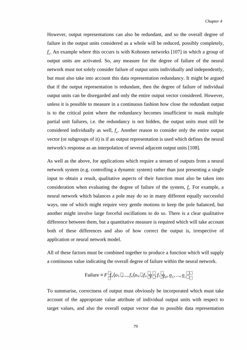
However, output representations can also be redundant, and so the overall degree of
failure in the output units considered as a whole will be reduced, possibly completely,
fo. An example where this occurs is with Kohonen networks [107] in which a group of
output units are activated. So, any measure for the degree of failure of the neural
network must not solely consider failure of output units individually and independently,
but must also take into account this data representation redundancy. It might be argued
that if the output representation is redundant, then the degree of failure of individual
output units can be disregarded and only the entire output vector considered. However,
unless it is possible to measure in a continuous fashion how close the redundant output
is to the critical point where the redundancy becomes insufficient to mask multiple
partial unit failures, i.e. the redundancy is not hidden, the output units must still be
considered individually as well, fu. Another reason to consider only the entire output
vector (or subgroups of it) is if an output representation is used which defines the neural
network's response as an interpolation of several adjacent output units [108].
As well as the above, for applications which require a stream of outputs from a neural
network system (e.g. controlling a dynamic system) rather than just presenting a single
input to obtain a result, qualitative aspects of their function must also be taken into
consideration when evaluating the degree of failure of the system, ft. For example, a
neural network which balances a pole may do so in many different equally successful
ways, one of which might require very gentle motions to keep the pole balanced, but
another might involve large forceful oscillations to do so. There is a clear qualitative
difference between them, but a quantitative measure is required which will take account
both of these differences and also of how correct the output is, irrespective of
application or neural network model.
All of these factors must be combined together to produce a function which will supply
a continuous value indicating the overall degree of failure within the neural network.
To summarise, correctness of output must obviously be incorporated which must take
account of the appropriate value attribute of individual output units with respect to
target values, and also the overall output vector due to possible data representation
Failure = Ffu(o1), ...,fu(on), fo
o
, f t o0, o1, ...,ot
Chapter 4
79
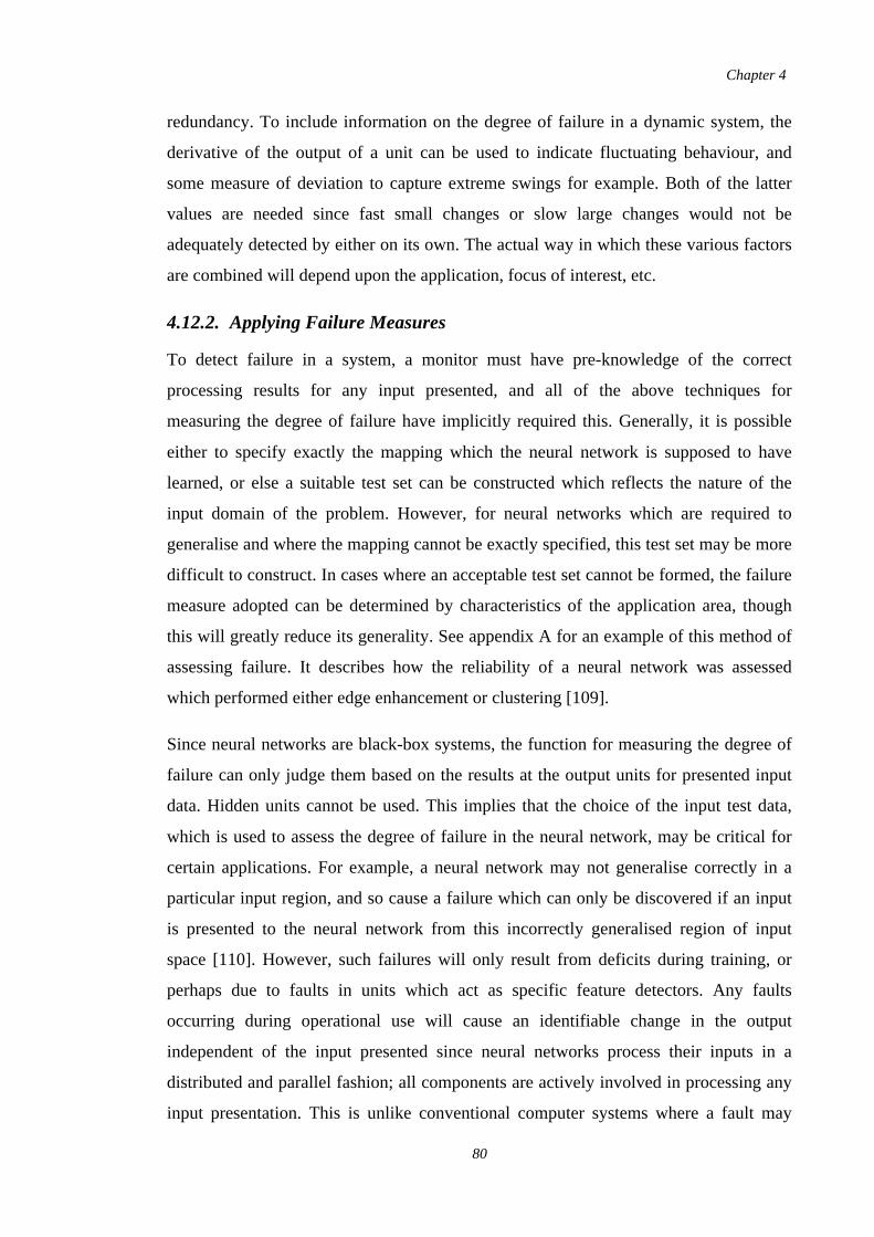
redundancy. To include information on the degree of failure in a dynamic system, the
derivative of the output of a unit can be used to indicate fluctuating behaviour, and
some measure of deviation to capture extreme swings for example. Both of the latter
values are needed since fast small changes or slow large changes would not be
adequately detected by either on its own. The actual way in which these various factors
are combined will depend upon the application, focus of interest, etc.
4.12.2. Applying Failure Measures
To detect failure in a system, a monitor must have pre-knowledge of the correct
processing results for any input presented, and all of the above techniques for
measuring the degree of failure have implicitly required this. Generally, it is possible
either to specify exactly the mapping which the neural network is supposed to have
learned, or else a suitable test set can be constructed which reflects the nature of the
input domain of the problem. However, for neural networks which are required to
generalise and where the mapping cannot be exactly specified, this test set may be more
difficult to construct. In cases where an acceptable test set cannot be formed, the failure
measure adopted can be determined by characteristics of the application area, though
this will greatly reduce its generality. See appendix A for an example of this method of
assessing failure. It describes how the reliability of a neural network was assessed
which performed either edge enhancement or clustering [109].
Since neural networks are black-box systems, the function for measuring the degree of
failure can only judge them based on the results at the output units for presented input
data. Hidden units cannot be used. This implies that the choice of the input test data,
which is used to assess the degree of failure in the neural network, may be critical for
certain applications. For example, a neural network may not generalise correctly in a
particular input region, and so cause a failure which can only be discovered if an input
is presented to the neural network from this incorrectly generalised region of input
space [110]. However, such failures will only result from deficits during training, or
perhaps due to faults in units which act as specific feature detectors. Any faults
occurring during operational use will cause an identifiable change in the output
independent of the input presented since neural networks process their inputs in a
distributed and parallel fashion; all components are actively involved in processing any
input presentation. This is unlike conventional computer systems where a fault may
Chapter 4
80
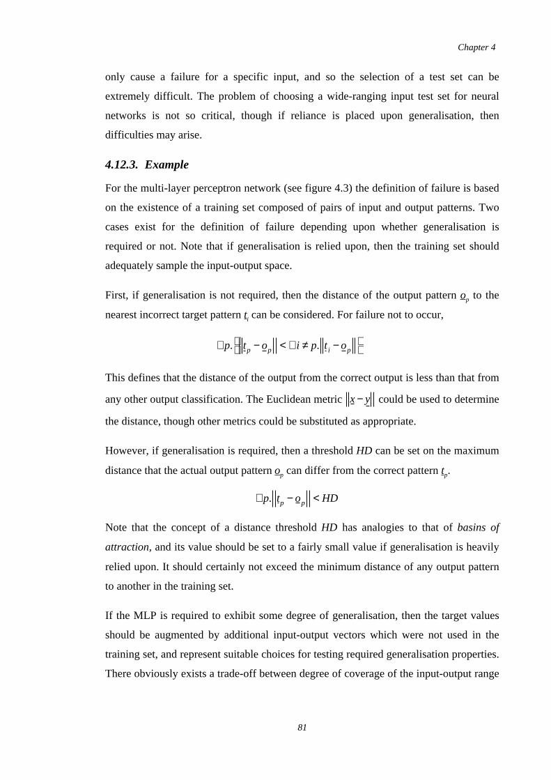
only cause a failure for a specific input, and so the selection of a test set can be
extremely difficult. The problem of choosing a wide-ranging input test set for neural
networks is not so critical, though if reliance is placed upon generalisation, then
difficulties may arise.
4.12.3. Example
For the multi-layer perceptron network (see figure 4.3) the definition of failure is based
on the existence of a training set composed of pairs of input and output patterns. Two
cases exist for the definition of failure depending upon whether generalisation is
required or not. Note that if generalisation is relied upon, then the training set should
adequately sample the input-output space.
First, if generalisation is not required, then the distance of the output pattern op to the
nearest incorrect target pattern ti can be considered. For failure not to occur,
This defines that the distance of the output from the correct output is less than that from
any other output classification. The Euclidean metric could be used to determinex− y
the distance, though other metrics could be substituted as appropriate.
However, if generalisation is required, then a threshold HD can be set on the maximum
distance that the actual output pattern op can differ from the correct pattern tp.
Note that the concept of a distance threshold HD has analogies to that of basins of
attraction, and its value should be set to a fairly small value if generalisation is heavily
relied upon. It should certainly not exceed the minimum distance of any output pattern
to another in the training set.
If the MLP is required to exhibit some degree of generalisation, then the target values
should be augmented by additional input-output vectors which were not used in the
training set, and represent suitable choices for testing required generalisation properties.
There obviously exists a trade-off between degree of coverage of the input-output range
∀ p. tp − op < ∀ i ≠ p. t i −op
∀ p. tp − op < HD
Chapter 4
81
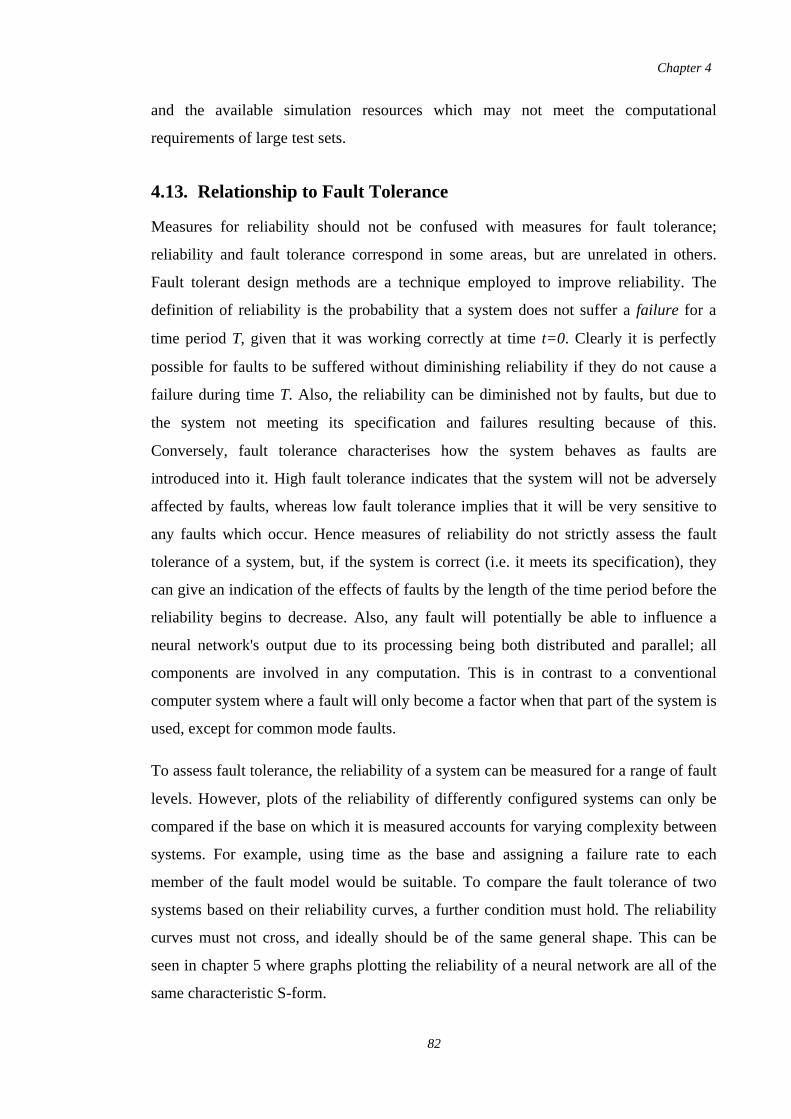
and the available simulation resources which may not meet the computational
requirements of large test sets.
4.13. Relationship to Fault Tolerance
Measures for reliability should not be confused with measures for fault tolerance;
reliability and fault tolerance correspond in some areas, but are unrelated in others.
Fault tolerant design methods are a technique employed to improve reliability. The
definition of reliability is the probability that a system does not suffer a failure for a
time period T, given that it was working correctly at time t=0. Clearly it is perfectly
possible for faults to be suffered without diminishing reliability if they do not cause a
failure during time T. Also, the reliability can be diminished not by faults, but due to
the system not meeting its specification and failures resulting because of this.
Conversely, fault tolerance characterises how the system behaves as faults are
introduced into it. High fault tolerance indicates that the system will not be adversely
affected by faults, whereas low fault tolerance implies that it will be very sensitive to
any faults which occur. Hence measures of reliability do not strictly assess the fault
tolerance of a system, but, if the system is correct (i.e. it meets its specification), they
can give an indication of the effects of faults by the length of the time period before the
reliability begins to decrease. Also, any fault will potentially be able to influence a
neural network's output due to its processing being both distributed and parallel; all
components are involved in any computation. This is in contrast to a conventional
computer system where a fault will only become a factor when that part of the system is
used, except for common mode faults.
To assess fault tolerance, the reliability of a system can be measured for a range of fault
levels. However, plots of the reliability of differently configured systems can only be
compared if the base on which it is measured accounts for varying complexity between
systems. For example, using time as the base and assigning a failure rate to each
member of the fault model would be suitable. To compare the fault tolerance of two
systems based on their reliability curves, a further condition must hold. The reliability
curves must not cross, and ideally should be of the same general shape. This can be
seen in chapter 5 where graphs plotting the reliability of a neural network are all of the
same characteristic S-form.
Chapter 4
82
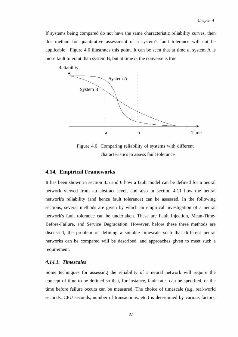
If systems being compared do not have the same characteristic reliability curves, then
this method for quantitative assessment of a system's fault tolerance will not be
applicable. Figure 4.6 illustrates this point. It can be seen that at time a, system A is
more fault tolerant than system B, but at time b, the converse is true.
4.14. Empirical Frameworks
It has been shown in section 4.5 and 6 how a fault model can be defined for a neural
network viewed from an abstract level, and also in section 4.11 how the neural
network's reliability (and hence fault tolerance) can be assessed. In the following
sections, several methods are given by which an empirical investigation of a neural
network's fault tolerance can be undertaken. These are Fault Injection, Mean-Time-
Before-Failure, and Service Degradation. However, before these three methods are
discussed, the problem of defining a suitable timescale such that different neural
networks can be compared will be described, and approaches given to meet such a
requirement.
4.14.1. Timescales
Some techniques for assessing the reliability of a neural network will require the
concept of time to be defined so that, for instance, fault rates can be specified, or the
time before failure occurs can be measured. The choice of timescale (e.g. real-world
seconds, CPU seconds, number of transactions, etc.) is determined by various factors,
Reliability
Time
System B
System A
ba
Figure 4.6 Comparing reliability of systems with different
characteristics to assess fault tolerance
Chapter 4
83
which are often in conflict with each other. Generally, the timescale should relate
sensibly to the characteristics of the application area, and to a lesser extent to the neural
network architecture used and the method of implementation.
For instance, a choice of measuring time in real-world seconds might be suitable for a
neural network system controlling some dynamical system, but not for a classification
application area where time would be better given the units of number of patterns
presented. Similarly, it would not be suitable to choose real-world seconds for a
software simulation of a neural network, CPU seconds or number of transactions would
be better. However, where a neural network model takes a non-deterministic number of
iterations to process an input (e.g. the Hopfield model), the units of time cannot be
based on a transaction count, but must rather be related to the number of iterations
performed by the system in evaluating an output, i.e. a measure that is invariant to
external controls or influences.
Not only must the timescale provide a suitable base from which to assess a particular
individual neural network's reliability, it must also allow valid comparisons to be made
between various different systems. These may or may not be based on the same neural
network model, and may even be non-neural systems. This means that the timescale
chosen must also take into account various factors such as the architecture and
implementation of the neural network model (e.g. evaluation algorithm, internal
components, etc.).
When comparing similar neural networks based on the same model all performing the
same task (e.g. MLP's with varying numbers of layers, hidden units), a large network
may well have better reliability when time is measured in number of pattern
presentations due to higher redundancy. However, an actual implementation of it will
take longer to process an input pattern than a smaller network performing the same task,
and so the number of faults occurring may well be greater in the long term. This
discrepancy should be compensated for in any comparative studies made. Producing
results that can be compared when using different types of neural network models or
non-neural systems requires similar consideration.
Two possible guidelines for choosing a timescale for a neural network system are either
examining the architecture and grouping together all of the parallel operations that are
Chapter 4
84
required during its processing stages, and then defining one unit of time to be the
execution (in parallel) of any particular group. The other possibility is to examine the
abstract description of the neural network model (e.g. see figure 4.3), and to define a
unit of time to be a recognizable mathematical operation. Both of these will allow
comparisons between the same neural networks model but with varying internal
structure, though to compare different (or non-deterministic) neural network models,
some allowance must be made for the complexity of operation for each possible time
unit such that the various models are evenly balanced.
4.14.2. Fault Injection Methods
Fault injection techniques involve subjecting a system to a known number of faults,
then measuring the subsequent degradation. This has to be repeated many times to
achieve a statistically significant result. The measure used to assess the system must be
related to the degree of failure of the system, since it is reliability which is of interest
here. Note that a system may maintain perfect performance until a fault threshold is
reached, when it suffers total failure. The discussion above on measuring the degree of
failure of a neural network is applicable here.
The resulting plots from experiments of the measure of reliability against many and
possibly various types of faults injected into a system, which can be termed fault
curves, will indicate how an operational system will behave if the rate at which each
type of fault occurs is known.
Fault injection techniques do suffer from a number of shortcomings. By far the most
damaging is when a system can suffer more than a single type of fault, as will almost
certainly be the case. Fault injection simulations are very good at indicating the isolated
effects of a number of identical faults occurring in a system, but are not effective in
analysing a system when many different fault types have to be taken into account since
their effects will not be independent. This makes it very difficult to predict with any
degree of accuracy the effects of various faults on a system which would occur in
real-life use. Combining in some fashion the effects of particular individual faults
occurring in isolation is very unlikely to be similar to the effects of all faults occurring
together over a period of time; the effects of individual fault types cannot simply be
added together due to correlations between them.
Chapter 4
85
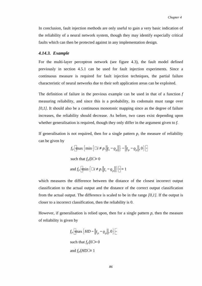
In conclusion, fault injection methods are only useful to gain a very basic indication of
the reliability of a neural network system, though they may identify especially critical
faults which can then be protected against in any implementation design.
4.14.3. Example
For the multi-layer perceptron network (see figure 4.3), the fault model defined
previously in section 4.5.1 can be used for fault injection experiments. Since a
continuous measure is required for fault injection techniques, the partial failure
characteristic of neural networks due to their soft application areas can be exploited.
The definition of failure in the previous example can be used in that of a function f
measuring reliability, and since this is a probability, its codomain must range over
[0,1]. It should also be a continuous monotonic mapping since as the degree of failure
increases, the reliability should decrease. As before, two cases exist depending upon
whether generalisation is required, though they only differ in the argument given to f.
If generalisation is not required, then for a single pattern p, the measure of reliability
can be given by
which measures the difference between the distance of the closest incorrect output
classification to the actual output and the distance of the correct output classification
from the actual output. The difference is scaled to be in the range [0,1]. If the output is
closer to a incorrect classification, then the reliability is 0.
However, if generalisation is relied upon, then for a single pattern p, then the measure
of reliability is given by
fp max min ∀ i ≠ p. t i − op − tp − op ,0
such that fp(0) = 0
and fp min ∀ i ≠ p. t i − op
= 1
fp max HD − tp − op ,0
such that fp(0) = 0
and fp(HD) = 1
Chapter 4
86
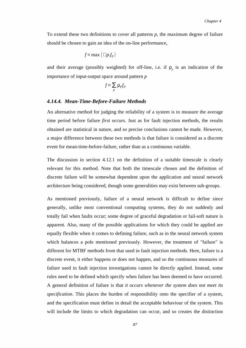
To extend these two definitions to cover all patterns p, the maximum degree of failure
should be chosen to gain an idea of the on-line performance,
and their average (possibly weighted) for off-line, i.e. if ρp is an indication of the
importance of input-output space around pattern p
4.14.4. Mean-Time-Before-Failure Methods
An alternative method for judging the reliability of a system is to measure the average
time period before failure first occurs. Just as for fault injection methods, the results
obtained are statistical in nature, and so precise conclusions cannot be made. However,
a major difference between these two methods is that failure is considered as a discrete
event for mean-time-before-failure, rather than as a continuous variable.
The discussion in section 4.12.1 on the definition of a suitable timescale is clearly
relevant for this method. Note that both the timescale chosen and the definition of
discrete failure will be somewhat dependent upon the application and neural network
architecture being considered, though some generalities may exist between sub-groups.
As mentioned previously, failure of a neural network is difficult to define since
generally, unlike most conventional computing systems, they do not suddenly and
totally fail when faults occur; some degree of graceful degradation or fail-soft nature is
apparent. Also, many of the possible applications for which they could be applied are
equally flexible when it comes to defining failure, such as in the neural network system
which balances a pole mentioned previously. However, the treatment of "failure" is
different for MTBF methods from that used in fault injection methods. Here, failure is a
discrete event, it either happens or does not happen, and so the continuous measures of
failure used in fault injection investigations cannot be directly applied. Instead, some
rules need to be defined which specify when failure has been deemed to have occurred.
A general definition of failure is that it occurs whenever the system does not meet its
specification. This places the burden of responsibility onto the specifier of a system,
and the specification must define in detail the acceptable behaviour of the system. This
will include the limits to which degradation can occur, and so creates the distinction
f = max ∀ p.fp
f = Σp
ρpfp
Chapter 4
87
between failure and non-failure. These limits can be defined using the various general
conditions that were discussed above for fault injection methods, though others which
are specific to the neural network or application may be included by the designer as
appropriate. For example, an output unit could be defined to have failed when its output
deviates by at least 20%. A more global definition might be that failure occurs when a
neural network incorrectly classifies more than 5% its inputs.
The basic MTBF technique can be extended when investigating neural networks to
assess the time between sequential failures since they can have the property of
automatic recovery from failures. This occurs since their functionality is unaffected by
errors in information processing caused either by transient faults or due to uneven
distribution of information. However, if feedback occurs in the neural network's
topology, then this might disrupt recovery since errors could be amplified.
In conclusion however, the rather gross simplification of failure from the continuous
degradation which actually occurs in a neural network to the discrete on-off event used
here, detracts from the usefulness of MTBF models for assessing the reliability of a
neural network system.
4.14.5. Example
To apply MTBF methods to the multi-layer perceptron (MLP) neural network, the
following requirements need to be met. A reasonable fault model needs to be
developed, a suitable timescale needs to be chosen, and also the notion of failure in the
MLP. The fault model defined earlier in section 4.5.1 can be applied here. A suitable
choice of timescale will depend to a large extent upon the application chosen, for a
classification problem, the timescale could relate to the number of patterns presented.
Failure can be treated similarly as in the above example, but replacing the function f by
one which jumps from 0 to 1 when the distance threshold HD is reached if
generalisation is relied upon, or else when the output pattern op is closer to tq where
if it is not.p ≠ q
By running many simulations, a plot of the cumulative number of simulation runs
against MTBF against the number of times a simulation has already failed (i.e. a 3D
graph) can be made. This will show the distribution of the MLP's failure rate, and also
Chapter 4
88
it will show how a system will behave after it has suffered N previous failures.
However, it will not indicate the degree of graceful degradation exhibited due to the
discrete failure event.
4.14.6. Service Degradation Methods
As mentioned above, both the fault injection and MTBF methods for measuring the
reliability of a neural network have their shortcomings. However, a combination of the
two methods can be devised which draws on their strengths, and removes their
associated problems. The continuous measures used in fault injection experiments are
combined with the timescales and fault rates of the extended MTBF methods to produce
a means by which to assess the global reliability of a neural network system as time
progresses. Since most neural networks exhibit graceful degradation, this method
provides a clear indication of impending catastrophe in the system.
To achieve a continuous-valued indication of the global reliability of the system, it is
possible to assign a probability to each particular fault mode which indicates both how
likely it will manifest itself in a single unit of time, and also the fraction of locations in
which it will occur. Faults can then be generated probabilistically during the simulation
run. It is important to take into account both of these factors since a fault which is
unlikely to occur, but has numerous fault locations could well be more likely to occur
than a highly probable fault that can only occur in a very few locations. By dynamically
generating various types of faults during the simulation, any correlations between their
effects will automatically be taken into account. The degree of failure in the system can
then be probed by using the reliability measures discussed above in section 4.10.1.
Similarly as for the MTBF reliability methods, another problem is that of choosing a
valid and reasonable timescale for faults and the discussion in section 4.12.1 applies
equally well here to service degradation methods. However, although this method
results in a clear picture of a neural network's graceful degradation of reliability, to
collect statistically meaningful results using this method, many simulation runs will
have to be performed, and the total computation cost could be very large. For
safety-critical systems though, failure would be far more costly.
Chapter 4
89

4.14.7. Example
By using the fault model developed earlier, the timescale as given in the example for
MTBF methods, and also the continuous reliability measure defined in the example for
fault injection techniques, the reliability of the MLP can be assessed. This is done by
running many simulations (to collect statistically valid data), placing faults
probabilistically according to the predefined fault rates, and measuring the reliability of
the MLP at each time step. This produces a plot of the reliability of the MLP against
time, and its performance can then be judged. Depending upon the generic nature of the
fault model, timescale and reliability measure used, the results obtained from various
different experiments (e.g. different size MLP's) can be compared and contrasted.
4.14.8. Summary of Simulation Frameworks
The three empirical simulation procedures given above are summarised below.
Fault Injection Procedure:
1. Train a neural network to final state and save parameters.
2. Start with fault-free trained neural network and choose single defect mode
from fault model:
3. Choose a (new) random location and apply defect.
4. Evaluate reliability of neural network.
5. Repeat from step 3 until some proportion of all possible locations
chosen.
6. Repeat from step 2 many times to average results.
Mean-Time-Before-Failure Procedure:
1. Train a neural network to final state and save parameters.
2. Start at time 0 with fault-free trained neural network and assign time-based
pdf to each mode in fault model:
3. For every possible fault location in neural network, apply pdf's to check
for defects.
4. Test whether neural network has failed. If so, record time and repeat
from step 2 until sufficient results obtained for MTBF.
Chapter 4
90
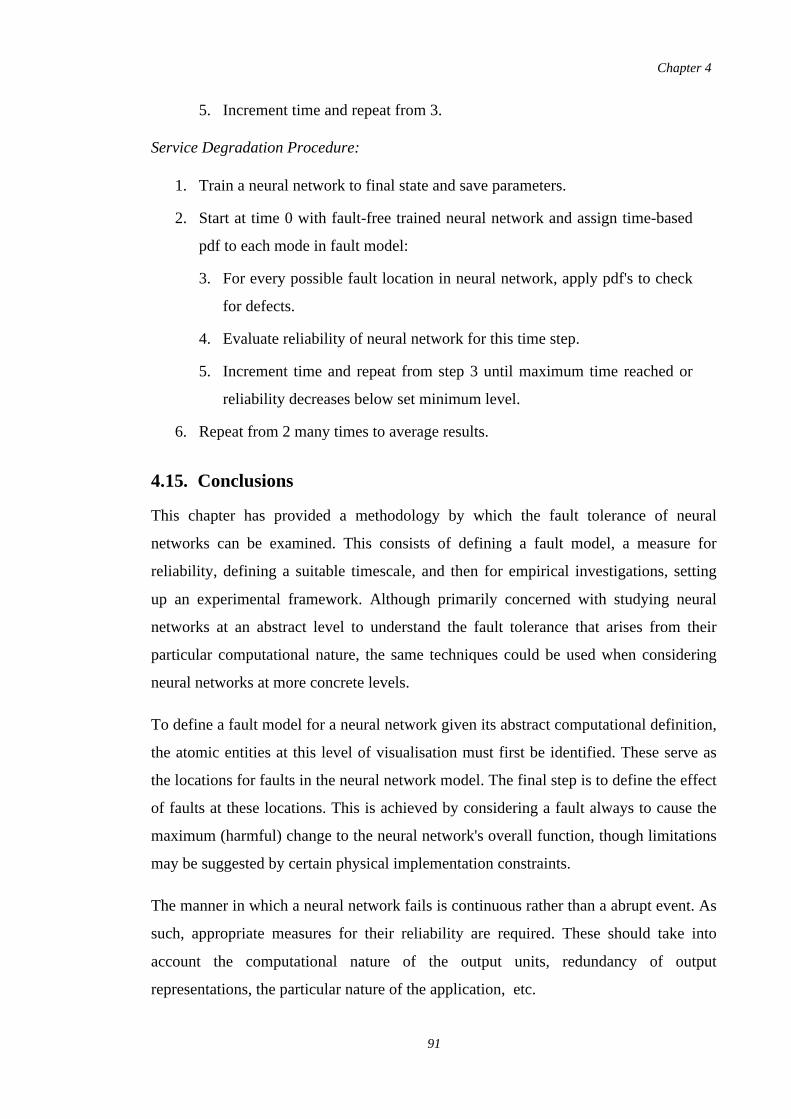
5. Increment time and repeat from 3.
Service Degradation Procedure:
1. Train a neural network to final state and save parameters.
2. Start at time 0 with fault-free trained neural network and assign time-based
pdf to each mode in fault model:
3. For every possible fault location in neural network, apply pdf's to check
for defects.
4. Evaluate reliability of neural network for this time step.
5. Increment time and repeat from step 3 until maximum time reached or
reliability decreases below set minimum level.
6. Repeat from 2 many times to average results.
4.15. Conclusions
This chapter has provided a methodology by which the fault tolerance of neural
networks can be examined. This consists of defining a fault model, a measure for
reliability, defining a suitable timescale, and then for empirical investigations, setting
up an experimental framework. Although primarily concerned with studying neural
networks at an abstract level to understand the fault tolerance that arises from their
particular computational nature, the same techniques could be used when considering
neural networks at more concrete levels.
To define a fault model for a neural network given its abstract computational definition,
the atomic entities at this level of visualisation must first be identified. These serve as
the locations for faults in the neural network model. The final step is to define the effect
of faults at these locations. This is achieved by considering a fault always to cause the
maximum (harmful) change to the neural network's overall function, though limitations
may be suggested by certain physical implementation constraints.
The manner in which a neural network fails is continuous rather than a abrupt event. As
such, appropriate measures for their reliability are required. These should take into
account the computational nature of the output units, redundancy of output
representations, the particular nature of the application, etc.
Chapter 4
91

Once both a fault model and reliability measure have been defined for a neural network,
the effect of faults on its operation can then be investigated using one of the three
simulation frameworks described above, i.e. fault injection, MTBF, or service
degradation. Fault injection is suitable for determining the consequence of a certain
fault on a neural network's operation. MTBF is applicable only if a neural network has a
abrupt failure mode imposed upon it. Service degradation is more useful since it
recognises that a neural network exhibits continuous failure.
In summary, this chapter has presented a methodology that allows the fault tolerance of
different neural network configurations, or even neural models, to be compared by
using the results obtained from simulations provided their failure curves are of the same
characteristic family.
Chapter 4
92
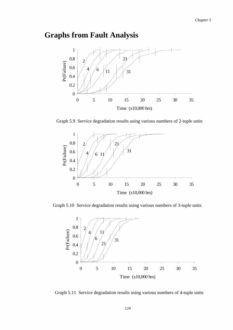
Graphs from Fault Analysis
Time (x10,000 hrs)
Pr(
Fa
ilure
)
0
0.2
0.4
0.6
0.8
1
0 5 10 15 20 25 30 35
2
4 6 11
21
31
Graph 5.9 Service degradation results using various numbers of 2-tuple units
Time (x10,000 hrs)
Pr(
Fa
ilure
)
0
0.2
0.4
0.6
0.8
1
0 5 10 15 20 25 30 35
2
4 6 11
21
31
Graph 5.10 Service degradation results using various numbers of 3-tuple units
Time (x10,000 hrs)
Pr(
Fa
ilure
)
0
0.2
0.4
0.6
0.8
1
0 5 10 15 20 25 30 35
24
611
2131
Chapter 5
124
Graph 5.11 Service degradation results using various numbers of 4-tuple units
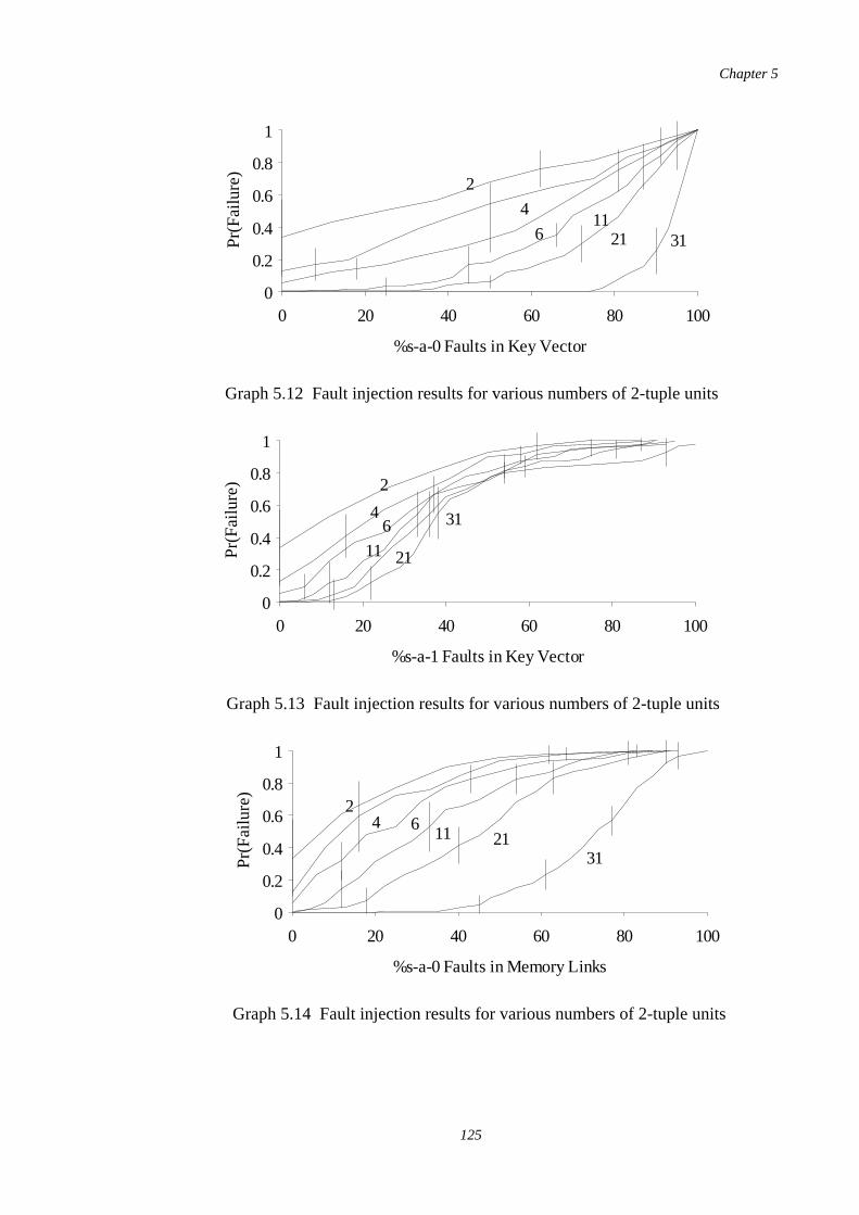
%s-a-0 Faults in Key Vector
Pr(
Fa
ilure
)
0
0.2
0.4
0.6
0.8
1
0 20 40 60 80 100
2
4
611
21 31
Graph 5.12 Fault injection results for various numbers of 2-tuple units
%s-a-1 Faults in Key Vector
Pr(
Fa
ilure
)
0
0.2
0.4
0.6
0.8
1
0 20 40 60 80 100
2
46
11 21
31
Graph 5.13 Fault injection results for various numbers of 2-tuple units
%s-a-0 Faults in Memory Links
Pr(
Fa
ilure
)
0
0.2
0.4
0.6
0.8
1
0 20 40 60 80 100
24 6
11 2131
Graph 5.14 Fault injection results for various numbers of 2-tuple units
Chapter 5
125
%s-a-1 Faults in Memory Links
Pr(
Fa
ilure
)
0
0.2
0.4
0.6
0.8
1
0 20 40 60 80 100
24 6
11 21
31
Graph 5.15 Fault injection results for various numbers of 2-tuple units
%s-a-0 Faults in Key Vector
Pr(
Fa
ilure
)
0
0.2
0.4
0.6
0.8
1
0 20 40 60 80 100
24 6 11 21 31
Graph 5.16 Fault injection results for various numbers of 3-tuple units
%s-a-1 Faults in Key Vector
Pr(
Fa
ilure
)
0
0.2
0.4
0.6
0.8
1
0 20 40 60 80 100
2
46
11
21
31
Graph 5.17 Fault injection results for various numbers of 3-tuple units
Chapter 5
126
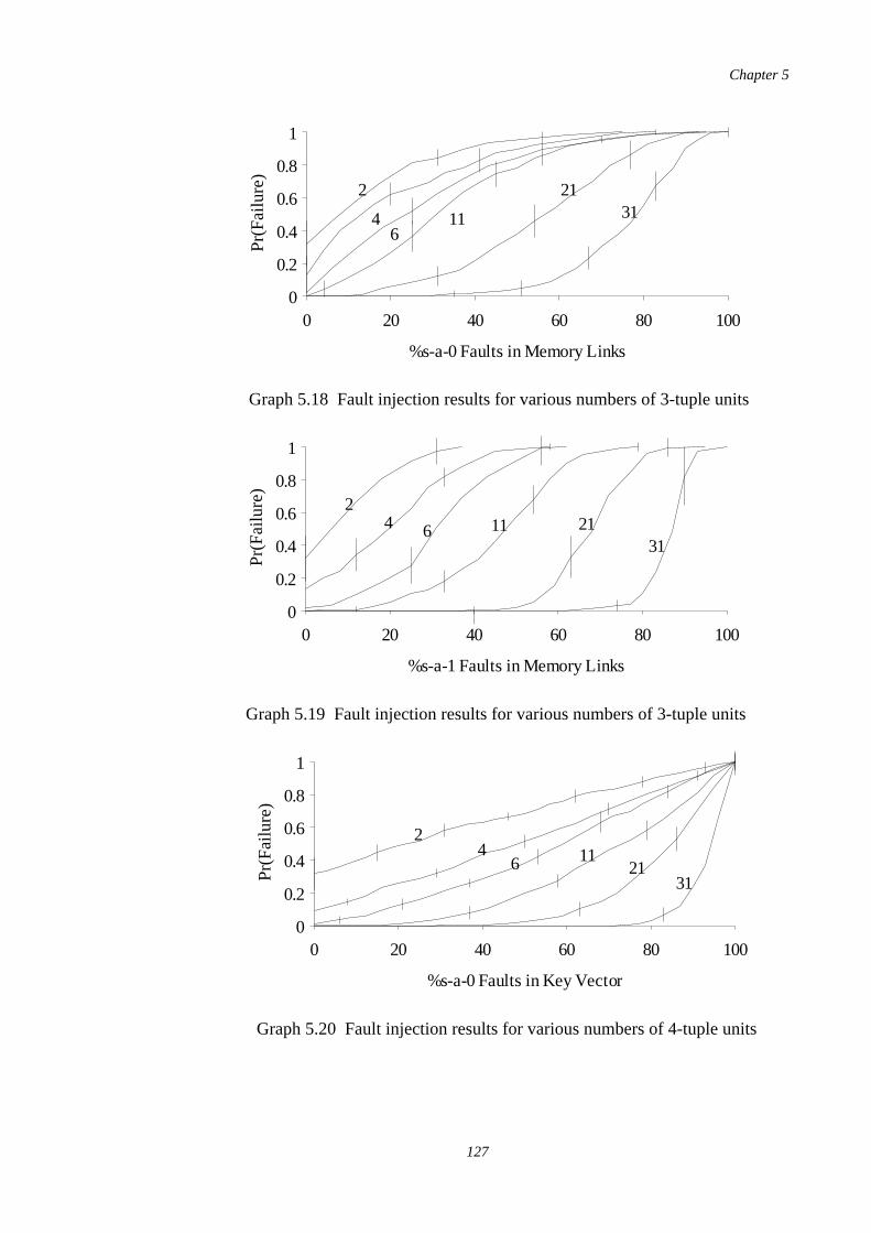
%s-a-0 Faults in Memory Links
Pr(
Fa
ilure
)
0
0.2
0.4
0.6
0.8
1
0 20 40 60 80 100
2
46
11
2131
Graph 5.18 Fault injection results for various numbers of 3-tuple units
%s-a-1 Faults in Memory Links
Pr(
Fa
ilure
)
0
0.2
0.4
0.6
0.8
1
0 20 40 60 80 100
24 6 11 21
31
Graph 5.19 Fault injection results for various numbers of 3-tuple units
%s-a-0 Faults in Key Vector
Pr(
Fa
ilure
)
0
0.2
0.4
0.6
0.8
1
0 20 40 60 80 100
24
6 1121
31
Graph 5.20 Fault injection results for various numbers of 4-tuple units
Chapter 5
127
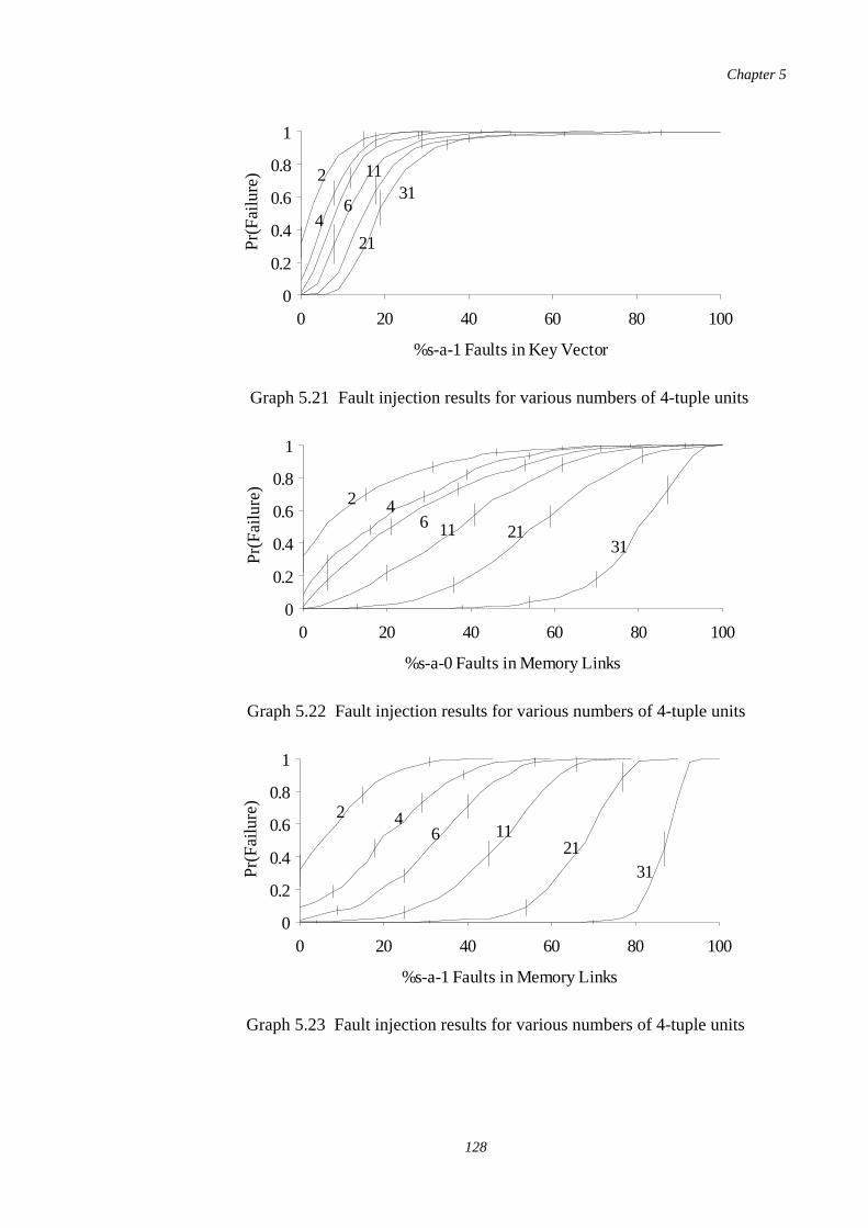
%s-a-1 Faults in Key Vector
Pr(
Fa
ilure
)
0
0.2
0.4
0.6
0.8
1
0 20 40 60 80 100
2
46
11
21
31
Graph 5.21 Fault injection results for various numbers of 4-tuple units
%s-a-0 Faults in Memory Links
Pr(
Fa
ilure
)
0
0.2
0.4
0.6
0.8
1
0 20 40 60 80 100
2 46 11 21
31
Graph 5.22 Fault injection results for various numbers of 4-tuple units
%s-a-1 Faults in Memory Links
Pr(
Fa
ilure
)
0
0.2
0.4
0.6
0.8
1
0 20 40 60 80 100
2 46 11
2131
Graph 5.23 Fault injection results for various numbers of 4-tuple units
Chapter 5
128
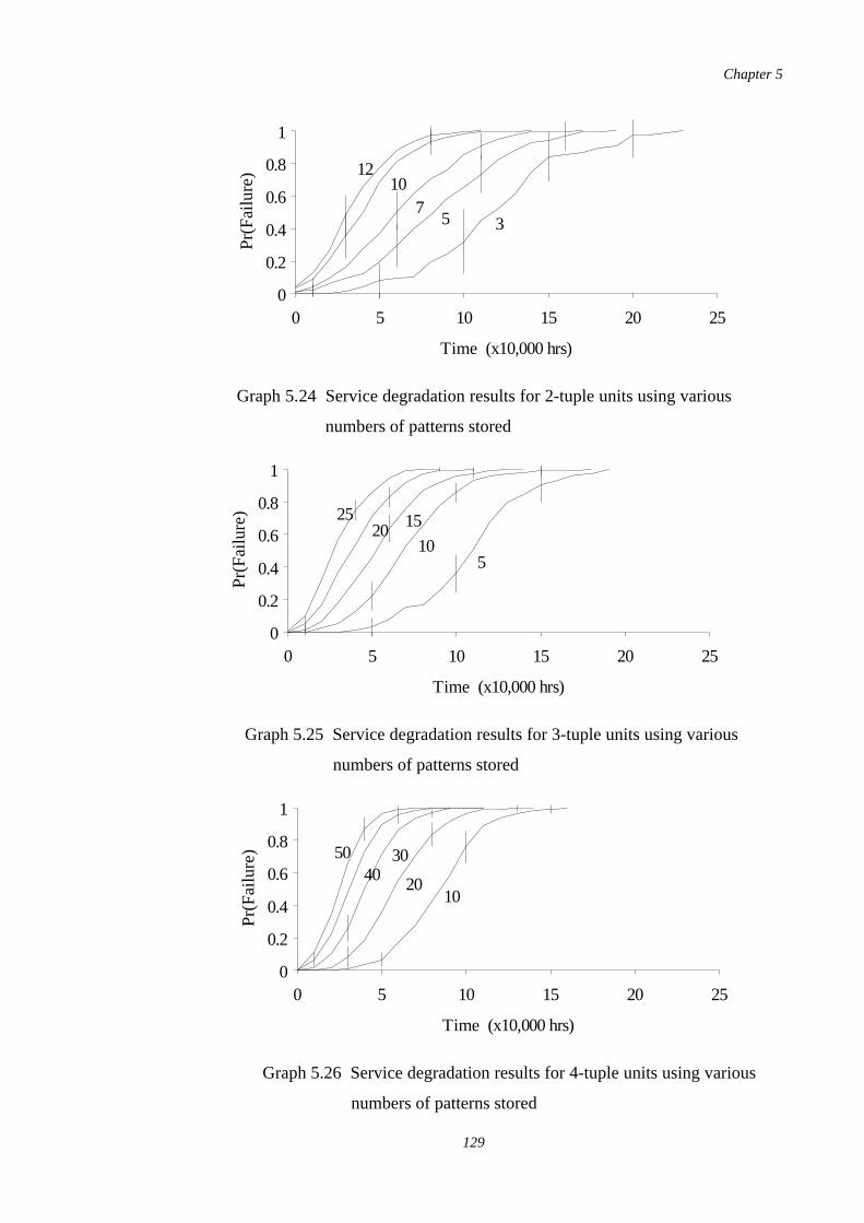
Time (x10,000 hrs)
Pr(
Fa
ilure
)
0
0.2
0.4
0.6
0.8
1
0 5 10 15 20 25
1210
75 3
Graph 5.24 Service degradation results for 2-tuple units using various
numbers of patterns stored
Time (x10,000 hrs)
Pr(
Fa
ilure
)
0
0.2
0.4
0.6
0.8
1
0 5 10 15 20 25
2520
15
105
Graph 5.25 Service degradation results for 3-tuple units using various
numbers of patterns stored
Time (x10,000 hrs)
Pr(
Fa
ilure
)
0
0.2
0.4
0.6
0.8
1
0 5 10 15 20 25
5040
30
2010
Graph 5.26 Service degradation results for 4-tuple units using various
numbers of patterns stored
Chapter 5
129
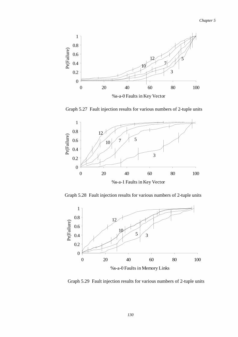
%s-a-0 Faults in Key Vector
Pr(
Fa
ilure
)
0
0.2
0.4
0.6
0.8
1
0 20 40 60 80 100
3
57
10
12
Graph 5.27 Fault injection results for various numbers of 2-tuple units
%s-a-1 Faults in Key Vector
Pr(
Fa
ilure
)
0
0.2
0.4
0.6
0.8
1
0 20 40 60 80 100
3
510 7
12
Graph 5.28 Fault injection results for various numbers of 2-tuple units
%s-a-0 Faults in Memory Links
Pr(
Fa
ilure
)
0
0.2
0.4
0.6
0.8
1
0 20 40 60 80 100
3510
12
Graph 5.29 Fault injection results for various numbers of 2-tuple units
Chapter 5
130
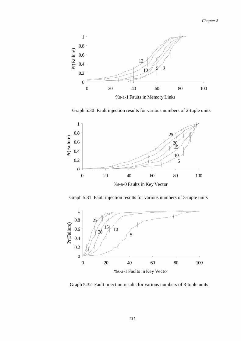
%s-a-1 Faults in Memory Links
Pr(
Fa
ilure
)
0
0.2
0.4
0.6
0.8
1
0 20 40 60 80 100
3510
12 7
Graph 5.30 Fault injection results for various numbers of 2-tuple units
%s-a-0 Faults in Key Vector
Pr(
Fa
ilure
)
0
0.2
0.4
0.6
0.8
1
0 20 40 60 80 100
510
20
25
15
Graph 5.31 Fault injection results for various numbers of 3-tuple units
%s-a-1 Faults in Key Vector
Pr(
Fa
ilure
)
0
0.2
0.4
0.6
0.8
1
0 20 40 60 80 100
510
20
2515
Graph 5.32 Fault injection results for various numbers of 3-tuple units
Chapter 5
131
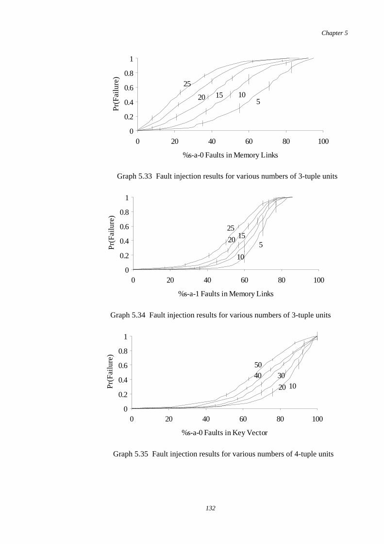
%s-a-0 Faults in Memory Links
Pr(
Fa
ilure
)
0
0.2
0.4
0.6
0.8
1
0 20 40 60 80 100
51020
25
15
Graph 5.33 Fault injection results for various numbers of 3-tuple units
%s-a-1 Faults in Memory Links
Pr(
Fa
ilure
)
0
0.2
0.4
0.6
0.8
1
0 20 40 60 80 100
5
10
20
2515
Graph 5.34 Fault injection results for various numbers of 3-tuple units
%s-a-0 Faults in Key Vector
Pr(
Fa
ilure
)
0
0.2
0.4
0.6
0.8
1
0 20 40 60 80 100
401020
3050
Graph 5.35 Fault injection results for various numbers of 4-tuple units
Chapter 5
132
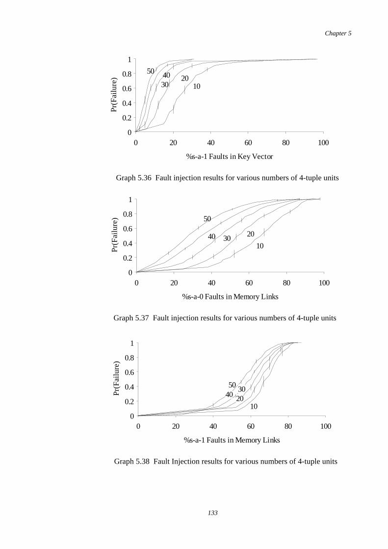
%s-a-1 Faults in Key Vector
Pr(
Fa
ilure
)
0
0.2
0.4
0.6
0.8
1
0 20 40 60 80 100
40
1020
30
50
Graph 5.36 Fault injection results for various numbers of 4-tuple units
%s-a-0 Faults in Memory Links
Pr(
Fa
ilure
)
0
0.2
0.4
0.6
0.8
1
0 20 40 60 80 100
4010
2030
50
Graph 5.37 Fault injection results for various numbers of 4-tuple units
%s-a-1 Faults in Memory Links
Pr(
Fa
ilure
)
0
0.2
0.4
0.6
0.8
1
0 20 40 60 80 100
5040
3020
10
Graph 5.38 Fault Injection results for various numbers of 4-tuple units
Chapter 5
133
CHAPTER SIX
Multi-Layer Perceptrons1
6.1. Introduction
Perceptrons were devised by McCulloch and Pitts in 1943 [62] as a crude model of
neurons in the brain. They are very simple computational devices which can perform
binary classification on linearly separable sets of data. A binary input vector is sampled
by a number of fixed predicate functions, whose weighted binary outputs are fed into a
threshold logic unit. There exists a training algorithm (Perceptron Learning Rule [62])
for linearly separable problems which is guaranteed to find the required weights that are
applied to each predicate output.
Due to the limited capabilities of the perceptron unit, an obvious advance was to
connect layers of perceptrons together. The perceptron units were simplified by only
allowing the first layer to have predicate functions sampling the input, if at all. This
architecture became known as a multi-layer perceptron network (MLP). However, it
was not clear how to train it since the original perceptron learning rule relied on
knowing the correct response for every unit given some input. For the internal units of a
multi-layer perceptron network this is not possible. This problem of spatial credit
assignment was a major stumbling block to neural network research in the late 60's. The
publication of Minsky and Papert's book [64] which comprehensively analysed
perceptron units and single layer networks composed from them discouraged many
researchers who were trying to develop learning algorithms for more complex neural
networks composed of many layers of perceptron units. However, in 1974 Werbos
[117] gave an algorithm which could train such a network, though continuous activation
functions were used instead of the original binary decision threshold. It was
subsequently rediscovered by other researchers including the Parallel Distributed
1 Part of this chapter has been published in [119].
Chapter 6
134
Processing (PDP) research group [21] in 1986 who termed the learning algorithm
Back-Error Propagation (BP).
This new learning algorithm has become almost synonymous with multi-layer
perceptron networks to such an extent that a clear distinction between the architecture
and learning algorithm has been lost in many cases. Back-error propagation is only one
particular method for configuring the weights in a MLP. The work presented in this
chapter leads to the conclusion that the back-error propagation algorithm is inherently
flawed with respect to developing neural networks exhibiting fault tolerance. However,
it will be seen later that it is possible to derive a set of weights which do lead to fault
tolerance.
Firstly section 6.2 describes how complex training sets used in the various simulations
were constructed. Section 6.3 then analyses the fault tolerance of perceptron units, and
experimental results are shown to support the theoretical model. Section 6.3.3 discusses
an alternative view than that of hyperplane separation of a perceptron's function.
Section 6.4 constructs a fault model for multi-layer perceptron networks. This is used in
section 6.5 to analyse the effect of faults on the functionality of a multi-layer perceptron
network. Section 6.6 then analyses the reliability of multi-layer perceptron networks
trained using back-error propagation, and methods of improving their rather poor
tolerance to faults given in section 6.7. Section 6.8 then analyses the resulting fault
tolerant multi-layer perceptron networks, and a new technique is developed which
produces similar networks at far less computational cost. Section 6.9 analyses the fault
tolerance of the MLP networks trained using the new algorithm, and the consequences
of this method for generalisation in multi-layer perceptron networks are given in section
6.10. Finally, section 6.11 examines properties of the hidden representations formed in
multi-layer perceptron networks with regard to their resilience to faults.
6.2. Construction of Training Sets
For the purposes of this study training sets were constructed artificially rather than
using a real data source. This allowed many training sessions to be performed quickly,
and more importantly, the characteristics of the data set to be fully known.
Chapter 6
135
An algorithm was devised which would produce a number of classes (c) with a number
of examples (cp) drawn from each class in a n-dimensional bipolar {-1,+1}n or binary
{0,1}n space. Each class centre was chosen randomly, but with the constraint that each
was a certain minimum distance from any other centre. This is required so that a certain
minimum number of pattern examples can definitely be chosen from every class. The
class centres can be viewed as pattern exemplars. The output patterns associated with
the inputs were of type 1 in c, i.e. 00010 would represent inputs sampled from the
second of 5 pattern exemplars.
The selection criterion for accepting a set of class centres was defined to be those cases
where the following inequality held:
It accepts any class set in which at least twice the number (p) of examples required from
each class could be found in the space owned by a particular class exemplar. This space
extends one half of the minimum interclass distance d. This condition is placed on
training set construction so that classes do not have too large a degree of overlap.
The example patterns drawn from each class were based on the class exemplar with
components randomly reversed with probability
This method selects pattern examples with high probability from the space owned by a
class exemplar, though it also allows for possible class overlap.
A seed value was specified for the pseudorandom number generator so that training sets
could be reproduced.
6.3. Perceptron Units
The operation of the simplified perceptron units used in multi-layer networks can be
described by the following equation
where ik is the kth input component, and wk is the weight on the connection from that
Σr=0
12d
nCr > 2p where d = min ci − cj ⋅ ∀ i ≠ j
Pr() =12
min ci − cj ⋅ ∀ i ≠ j
n
output = σ Σk=1
n
i kwk − θ
= σ i ⋅ w− θ
(6.1)
Chapter 6
136
input. The constant θ offsets the weight input sum, and is normally termed the bias. The
function σ applied to the final result of the summation (activation) generally maps it
into a limited range [a,b], and hence is often called a squashing function.
The function of a perceptron unit is to classify its inputs into two classes, possibly with
some notion of certainty added. This is a crude model of the behaviour of neurons in
the brain which given certain stimuli, fire in bursts with frequency relating to the
closeness of the input stimulus to its exemplar [118].
There are three main classes of squashing function (σ) which have been developed and
used in perceptron units:
Binary: The output of units is hard-limited to binary {0,1} or bipolar {-1,+1}
values.
Linear: The squashing function maps x to ax. Generally the output represents
two classes based on the sign of the output, and the absolute magnitude
the certainty of response.
Non-Linear: The activation is mapped to a limited range as with the binary units,
though here the mapping is continuous. In accordance with the notion of
a perceptron unit representing two classes, the function tends to be
monotonically increasing. This is the class of units employed in MLP
networks.
6.3.1. Fault Tolerance of Perceptron Units
This section examines the fault tolerance arising from a perceptron unit's style of
computation. First, a simple fault model will be constructed. From equation 6.1 it can
be seen that the majority of entities in a unit occur in the summation of weight and
input components. Since the number of weights far outweighs the single bias θ, then it
can be considered to be masked by the weighted summation terms if its value is no
larger than typical weight values. However, if this is not the case, then since the bias is
often considered as being a weight from a unit with fixed output -1, it could be included
without special provision as an extra summation term.
Chapter 6
137
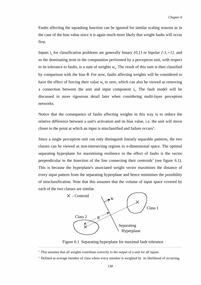
Faults affecting the squashing function can be ignored for similar scaling reasons as in
the case of the bias value since it is again much more likely that weight faults will occur
first.
Inputs ik for classification problems are generally binary {0,1} or bipolar {-1,+1}, and
so the dominating term in the computation performed by a perceptron unit, with respect
to its tolerance to faults, is a sum of weights wk. The result of this sum is then classified
by comparison with the bias θ. For now, faults affecting weights will be considered to
have the effect of forcing their value wk to zero, which can also be viewed as removing
a connection between the unit and input component ik. The fault model will be
discussed in more rigourous detail later when considering multi-layer perceptron
networks.
Notice that the consequence of faults affecting weights in this way is to reduce the
relative difference between a unit's activation and its bias value, i.e. the unit will move
closer to the point at which an input is misclassified and failure occurs2.
Since a single perceptron unit can only distinguish linearly separable patterns, the two
classes can be viewed as non-intersecting regions in n-dimensional space. The optimal
separating hyperplane for maximising resilience to the effect of faults is the vector
perpendicular to the bisection of the line connecting their centroids3 (see figure 6.1).
This is because the hyperplane's associated weight vector maximises the distance of
every input pattern from the separating hyperplane and hence minimises the possibility
of misclassification. Note that this assumes that the volume of input space covered by
each of the two classes are similar.
2 This assumes that all weights contribute correctly to the output of a unit for all inputs.3 Defined as average member of class where every member is weighted by its likelihood of occurring.
- Centroid
SeparatingHyperplane
Class 1
Class 2
w
θ
Figure 6.1 Separating hyperplane for maximal fault tolerance
Chapter 6
138
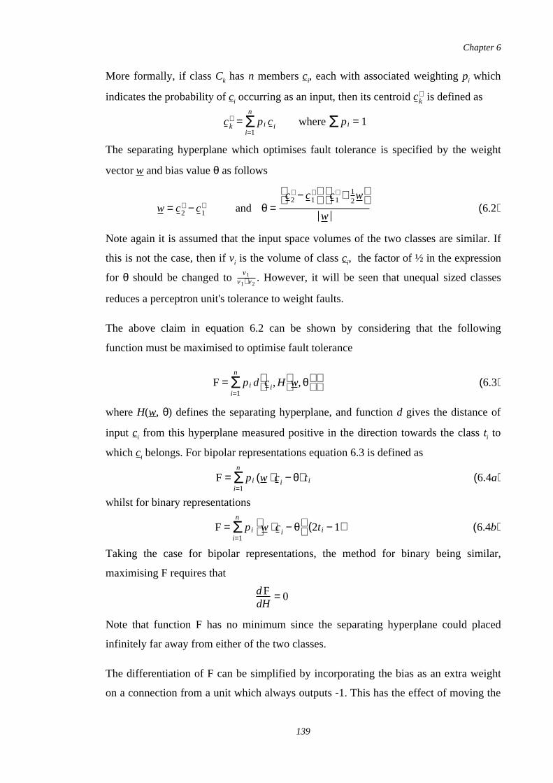
More formally, if class Ck has n members ci, each with associated weighting pi which
indicates the probability of ci occurring as an input, then its centroid is defined asck∗
The separating hyperplane which optimises fault tolerance is specified by the weight
vector w and bias value θ as follows
Note again it is assumed that the input space volumes of the two classes are similar. If
this is not the case, then if vi is the volume of class ci, the factor of ½ in the expression
for θ should be changed to . However, it will be seen that unequal sized classesv1v1+v2
reduces a perceptron unit's tolerance to weight faults.
The above claim in equation 6.2 can be shown by considering that the following
function must be maximised to optimise fault tolerance
where H(w, θ) defines the separating hyperplane, and function d gives the distance of
input ci from this hyperplane measured positive in the direction towards the class ti to
which ci belongs. For bipolar representations equation 6.3 is defined as
whilst for binary representations
Taking the case for bipolar representations, the method for binary being similar,
maximising F requires that
Note that function F has no minimum since the separating hyperplane could placed
infinitely far away from either of the two classes.
The differentiation of F can be simplified by incorporating the bias as an extra weight
on a connection from a unit which always outputs -1. This has the effect of moving the
ck∗ = Σ
i=1
n
pi ci whereΣ pi = 1
w = c2∗ −c1
∗ and θ = c2
∗ − c1∗
c1
∗ + 12w
w
(6.2)
F = Σi=1
n
pi d ci ,H
w,θ
(6.3)
F = Σi=1
n
pi (w ⋅ ci −θ) t i (6.4a)
F = Σi=1
n
pi w ⋅ ci − θ
(2t i −1) (6.4b)
dFdH
= 0
Chapter 6
139
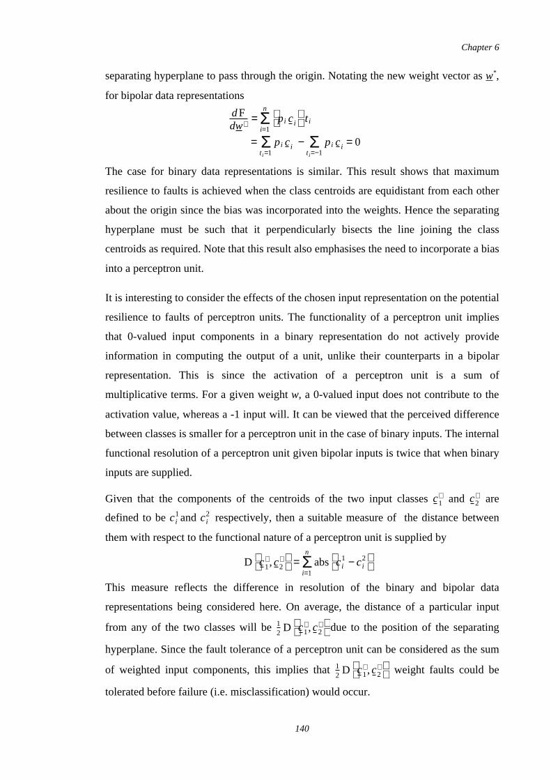
separating hyperplane to pass through the origin. Notating the new weight vector as w*,
for bipolar data representations
The case for binary data representations is similar. This result shows that maximum
resilience to faults is achieved when the class centroids are equidistant from each other
about the origin since the bias was incorporated into the weights. Hence the separating
hyperplane must be such that it perpendicularly bisects the line joining the class
centroids as required. Note that this result also emphasises the need to incorporate a bias
into a perceptron unit.
It is interesting to consider the effects of the chosen input representation on the potential
resilience to faults of perceptron units. The functionality of a perceptron unit implies
that 0-valued input components in a binary representation do not actively provide
information in computing the output of a unit, unlike their counterparts in a bipolar
representation. This is since the activation of a perceptron unit is a sum of
multiplicative terms. For a given weight w, a 0-valued input does not contribute to the
activation value, whereas a -1 input will. It can be viewed that the perceived difference
between classes is smaller for a perceptron unit in the case of binary inputs. The internal
functional resolution of a perceptron unit given bipolar inputs is twice that when binary
inputs are supplied.
Given that the components of the centroids of the two input classes and arec1∗ c2
∗
defined to be and respectively, then a suitable measure of the distance betweenci1 ci
2
them with respect to the functional nature of a perceptron unit is supplied by
This measure reflects the difference in resolution of the binary and bipolar data
representations being considered here. On average, the distance of a particular input
from any of the two classes will be due to the position of the separating12
D c1
∗ ,c2∗
hyperplane. Since the fault tolerance of a perceptron unit can be considered as the sum
of weighted input components, this implies that weight faults could be12
D c1
∗ ,c2∗
tolerated before failure (i.e. misclassification) would occur.
dFdw∗ = Σ
i=1
n pi ci
t i
= Σt i =1
pi ci − Σt i=−1
pi ci = 0
D c1
∗ ,c2∗ = Σ
i=1
n
abs ci
1 − ci2
Chapter 6
140
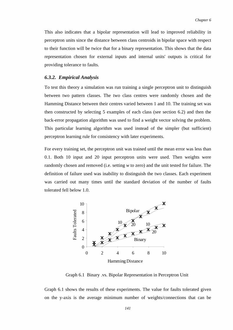
This also indicates that a bipolar representation will lead to improved reliability in
perceptron units since the distance between class centroids in bipolar space with respect
to their function will be twice that for a binary representation. This shows that the data
representation chosen for external inputs and internal units' outputs is critical for
providing tolerance to faults.
6.3.2. Empirical Analysis
To test this theory a simulation was run training a single perceptron unit to distinguish
between two pattern classes. The two class centres were randomly chosen and the
Hamming Distance between their centres varied between 1 and 10. The training set was
then constructed by selecting 5 examples of each class (see section 6.2) and then the
back-error propagation algorithm was used to find a weight vector solving the problem.
This particular learning algorithm was used instead of the simpler (but sufficient)
perceptron learning rule for consistency with later experiments.
For every training set, the perceptron unit was trained until the mean error was less than
0.1. Both 10 input and 20 input perceptron units were used. Then weights were
randomly chosen and removed (i.e. setting w to zero) and the unit tested for failure. The
definition of failure used was inability to distinguish the two classes. Each experiment
was carried out many times until the standard deviation of the number of faults
tolerated fell below 1.0.
Graph 6.1 shows the results of these experiments. The value for faults tolerated given
on the y-axis is the average minimum number of weights/connections that can be
Hamming Distance
Fa
ults
To
lera
ted
0
2
4
6
8
10
0 2 4 6 8 10
10 20
20
10
Binary
Bipolar
Graph 6.1 Binary .vs. Bipolar Representation in Perceptron Unit
Chapter 6
141
removed without failure occurring. This is plotted against a data set's Hamming
Distance between class centres. It can be seen that the data collected closely matches the
theoretical predictions (marked with stars). Also, it clearly shows that bipolar
representations lead to improved tolerance to faults as expected above.
6.3.3. Alternative Visualisation of a Perceptron's Function
The predominant technique for visualising the operation of a perceptron unit is by
considering that it classifies patterns based on a dichotomy of its input space. This is
formed by a hyperplane which is normal to the weight vector w and distance θ from the
origin. An alternative understanding of a perceptron unit's computation at a lower
functional level is more appropriate in this chapter. A unit's function is viewed in terms
of its internal operation rather than by its output representation. Although both
visualisations precisely describe the operation of a perceptron unit, hyperplane
separation does not naturally extend to allow intuitive insight into visualising the effect
of faults, as was seen in the previous section.
The alternative concept proposed here for visualising a perceptron unit's computation
starts from considering the scalar value of the vector projection of input x onto weight
vector w. It can be viewed that this indicates the degree by which x matches w. This
value is then compared to the bias θ, and the output of the unit indicates if the match
was sufficient.
The weight vector w defines the feature which the perceptron unit represents in a subset
of its input space. A subset is specified since it has been found that not all the weights
on connections feeding a unit are used, some decay to near zero during training and
play no significant part in the units operation4. Note that by the term feature used
above, it is not meant that a unit's weight vector corresponds to some semantic object in
the problem domain.
The bias represents by what degree the feature represented by the weight vector
represents has to be present in the input x. If there is enough evidence, i.e. w.x > θ, then
it will cause the unit to "fire". A non-linear squashing function saturates the unit's
activation as appropriate.
4 This is the basis for the various pruning algorithms which have been developed [60].
Chapter 6
142
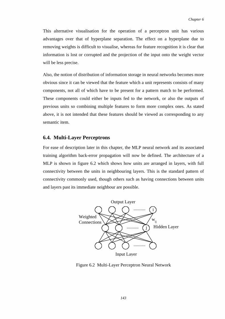
This alternative visualisation for the operation of a perceptron unit has various
advantages over that of hyperplane separation. The effect on a hyperplane due to
removing weights is difficult to visualise, whereas for feature recognition it is clear that
information is lost or corrupted and the projection of the input onto the weight vector
will be less precise.
Also, the notion of distribution of information storage in neural networks becomes more
obvious since it can be viewed that the feature which a unit represents consists of many
components, not all of which have to be present for a pattern match to be performed.
These components could either be inputs fed to the network, or also the outputs of
previous units so combining multiple features to form more complex ones. As stated
above, it is not intended that these features should be viewed as corresponding to any
semantic item.
6.4. Multi-Layer Perceptrons
For ease of description later in this chapter, the MLP neural network and its associated
training algorithm back-error propagation will now be defined. The architecture of a
MLP is shown in figure 6.2 which shows how units are arranged in layers, with full
connectivity between the units in neighbouring layers. This is the standard pattern of
connectivity commonly used, though others such as having connections between units
and layers past its immediate neighbour are possible.
Input Layer
Output Layer
..........
..........
..........
Hidden Layer
WeightedConnections
i
j
wi j
Figure 6.2 Multi-Layer Perceptron Neural Network
Chapter 6
143
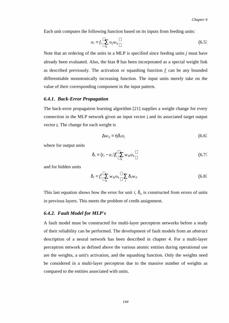
Each unit computes the following function based on its inputs from feeding units:
Note that an ordering of the units in a MLP is specified since feeding units j must have
already been evaluated. Also, the bias θ has been incorporated as a special weight link
as described previously. The activation or squashing function fi can be any bounded
differentiable monotonically increasing function. The input units merely take on the
value of their corresponding component in the input pattern.
6.4.1. Back-Error Propagation
The back-error propagation learning algorithm [21] supplies a weight change for every
connection in the MLP network given an input vector i and its associated target output
vector t. The change for each weight is
where for output units
and for hidden units
This last equation shows how the error for unit i, δi, is constructed from errors of units
in previous layers. This meets the problem of credit assignment.
6.4.2. Fault Model for MLP's
A fault model must be constructed for multi-layer perceptron networks before a study
of their reliability can be performed. The development of fault models from an abstract
description of a neural network has been described in chapter 4. For a multi-layer
perceptron network as defined above the various atomic entities during operational use
are the weights, a unit's activation, and the squashing function. Only the weights need
be considered in a multi-layer perceptron due to the massive number of weights as
compared to the entities associated with units.
oi = f i Σk ojwij
(6.5)
∆wij = ηδioj (6.6)
δi = (t i −oi)f i Σk wikok
(6.7)
δi = f i Σk wikok
Σ
lδlwil (6.8)
Chapter 6
144
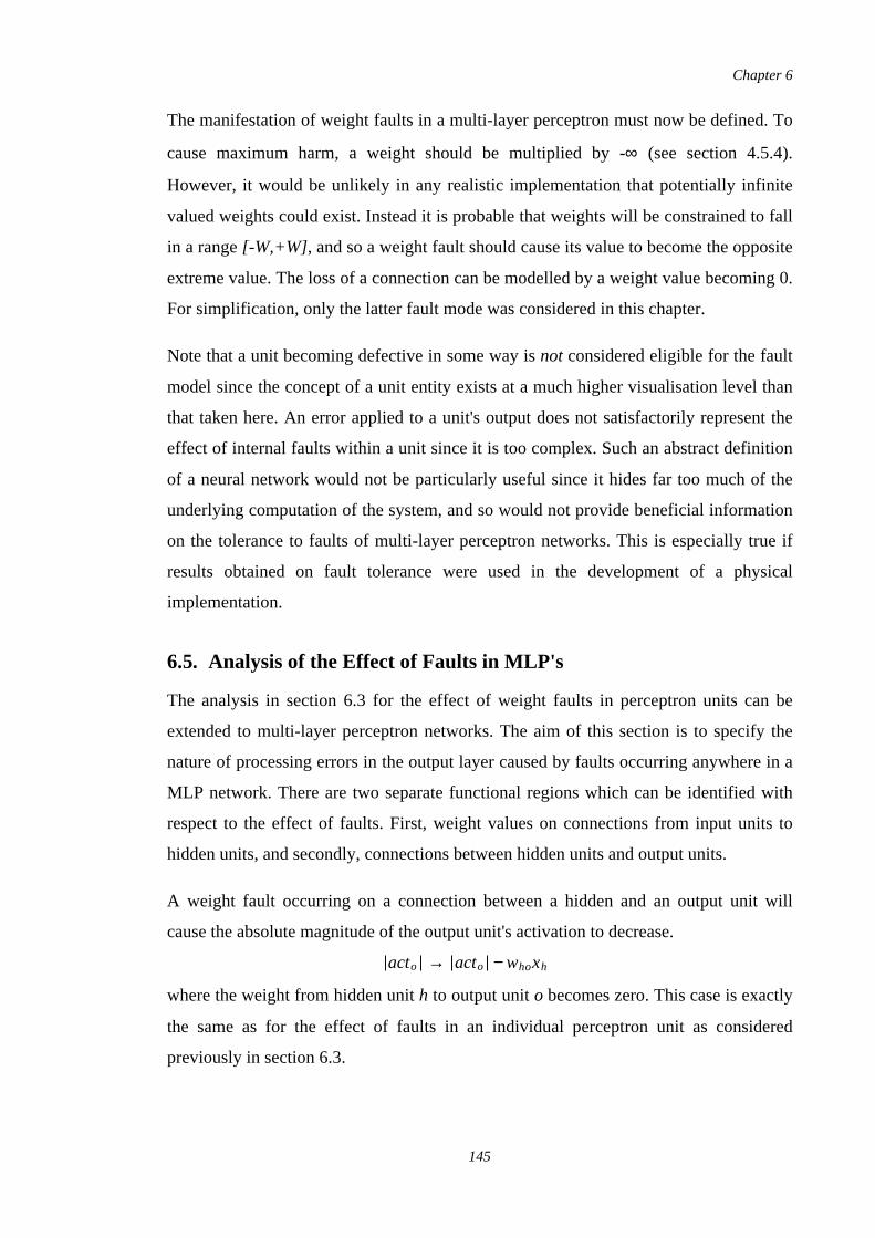
The manifestation of weight faults in a multi-layer perceptron must now be defined. To
cause maximum harm, a weight should be multiplied by -∞ (see section 4.5.4).
However, it would be unlikely in any realistic implementation that potentially infinite
valued weights could exist. Instead it is probable that weights will be constrained to fall
in a range [-W,+W], and so a weight fault should cause its value to become the opposite
extreme value. The loss of a connection can be modelled by a weight value becoming 0.
For simplification, only the latter fault mode was considered in this chapter.
Note that a unit becoming defective in some way is not considered eligible for the fault
model since the concept of a unit entity exists at a much higher visualisation level than
that taken here. An error applied to a unit's output does not satisfactorily represent the
effect of internal faults within a unit since it is too complex. Such an abstract definition
of a neural network would not be particularly useful since it hides far too much of the
underlying computation of the system, and so would not provide beneficial information
on the tolerance to faults of multi-layer perceptron networks. This is especially true if
results obtained on fault tolerance were used in the development of a physical
implementation.
6.5. Analysis of the Effect of Faults in MLP's
The analysis in section 6.3 for the effect of weight faults in perceptron units can be
extended to multi-layer perceptron networks. The aim of this section is to specify the
nature of processing errors in the output layer caused by faults occurring anywhere in a
MLP network. There are two separate functional regions which can be identified with
respect to the effect of faults. First, weight values on connections from input units to
hidden units, and secondly, connections between hidden units and output units.
A weight fault occurring on a connection between a hidden and an output unit will
cause the absolute magnitude of the output unit's activation to decrease.
where the weight from hidden unit h to output unit o becomes zero. This case is exactly
the same as for the effect of faults in an individual perceptron unit as considered
previously in section 6.3.
acto → acto − whoxh
Chapter 6
145
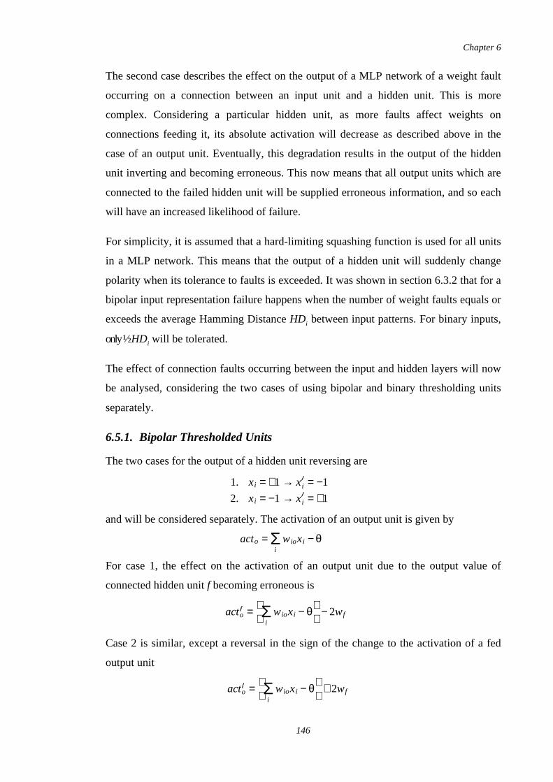
The second case describes the effect on the output of a MLP network of a weight fault
occurring on a connection between an input unit and a hidden unit. This is more
complex. Considering a particular hidden unit, as more faults affect weights on
connections feeding it, its absolute activation will decrease as described above in the
case of an output unit. Eventually, this degradation results in the output of the hidden
unit inverting and becoming erroneous. This now means that all output units which are
connected to the failed hidden unit will be supplied erroneous information, and so each
will have an increased likelihood of failure.
For simplicity, it is assumed that a hard-limiting squashing function is used for all units
in a MLP network. This means that the output of a hidden unit will suddenly change
polarity when its tolerance to faults is exceeded. It was shown in section 6.3.2 that for a
bipolar input representation failure happens when the number of weight faults equals or
exceeds the average Hamming Distance HDi between input patterns. For binary inputs,
only ½HDi will be tolerated.
The effect of connection faults occurring between the input and hidden layers will now
be analysed, considering the two cases of using bipolar and binary thresholding units
separately.
6.5.1. Bipolar Thresholded Units
The two cases for the output of a hidden unit reversing are
and will be considered separately. The activation of an output unit is given by
For case 1, the effect on the activation of an output unit due to the output value of
connected hidden unit f becoming erroneous is
Case 2 is similar, except a reversal in the sign of the change to the activation of a fed
output unit
1. xi = +1 → xi = −1
2. xi = −1 → xi = +1
acto = Σi
wioxi −θ
acto = Σi
wioxi − θ
− 2wf
acto = Σi
wioxi − θ
+ 2wf
Chapter 6
146
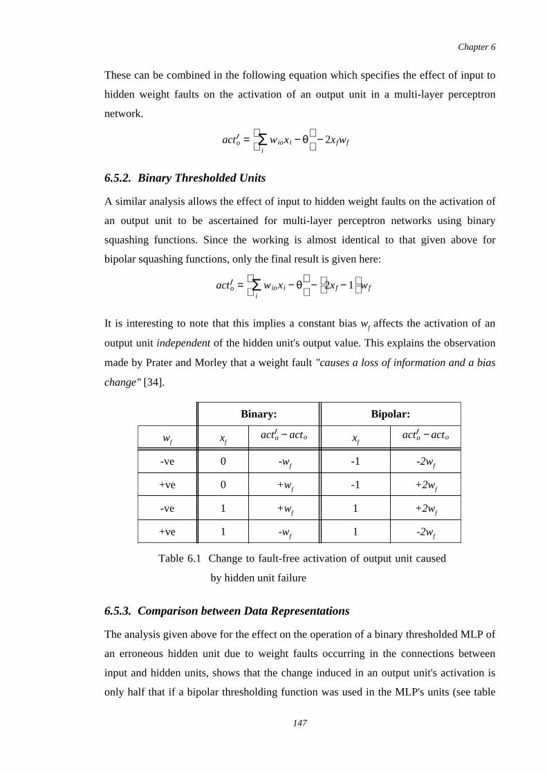
These can be combined in the following equation which specifies the effect of input to
hidden weight faults on the activation of an output unit in a multi-layer perceptron
network.
6.5.2. Binary Thresholded Units
A similar analysis allows the effect of input to hidden weight faults on the activation of
an output unit to be ascertained for multi-layer perceptron networks using binary
squashing functions. Since the working is almost identical to that given above for
bipolar squashing functions, only the final result is given here:
It is interesting to note that this implies a constant bias wf affects the activation of an
output unit independent of the hidden unit's output value. This explains the observation
made by Prater and Morley that a weight fault "causes a loss of information and a bias
change" [34].
Binary: Bipolar:
wf xfacto − acto xf
acto −acto
-ve 0 -wf -1 -2wf
+ve 0 +wf -1 +2wf
-ve 1 +wf 1 +2wf
+ve 1 -wf 1 -2wf
6.5.3. Comparison between Data Representations
The analysis given above for the effect on the operation of a binary thresholded MLP of
an erroneous hidden unit due to weight faults occurring in the connections between
input and hidden units, shows that the change induced in an output unit's activation is
only half that if a bipolar thresholding function was used in the MLP's units (see table
acto = Σi
wioxi − θ
− 2xfwf
acto = Σi
wioxi − θ
− 2xf − 1
wf
Table 6.1 Change to fault-free activation of output unit caused
by hidden unit failure
Chapter 6
147
6.1). This suggests that a binary thresholding method should be used for all of the units
in a MLP network. However, using a binary threshold method would also have the
consequence of halving the number of weight faults which could be tolerated by
individual units in their incoming connections (c.f. section 6.3.2), and so the decision of
which data representation for the thresholding function to use is not trivial.
The two cases of using either bipolar or binary squashing functions in a MLP network
will now be considered separately. Note that HDi is the average Hamming Distance
between input patterns, and HDh is the average Hamming Distance between
representations formed in the hidden layer of a MLP.
First, if a bipolar squashing function is used in a MLP, then for an output unit to just
fail, either ½HDh hidden units must fail, or HDh hidden to output weight faults must
occur, or else some combination of these two events must occur:
However, if binary squashing functions are used, then either ½HDh hidden units must fail
(as before), or ½HDh hidden-output weight faults must occur. The various combinations
of these two events can be expressed as
It can be seen that a MLP network using bipolar squashing functions will exhibit better
tolerance to faults than the case when binary squashing functions are used. This
conclusion is drawn by noting that in both cases an equal number of hidden unit failures
causes similar damage to the function of output units. However, binary thresholded
hidden units are more likely to fail since they will only tolerate ½HDi faults in their input
connections, while bipolar thresholded hidden units will tolerate HDi weight faults.
6.5.4. Conversion of Binary to Bipolar Thresholded MLP
A trained MLP which employs binary thresholded units can easily be transformed into
an equivalent MLP with bipolar units. However, although the function of the MLP will
remain unchanged, the results given above imply that its reliability will be greatly
increased due to the improvement in the fault tolerance of its individual units.
i hidden units fail ∧HDh −2i hidden-output weight faults
i = 0...12HDh
i hidden units fail ∧
12HDh − i hidden-output weight faults
i = 0...12HDh
Chapter 6
148
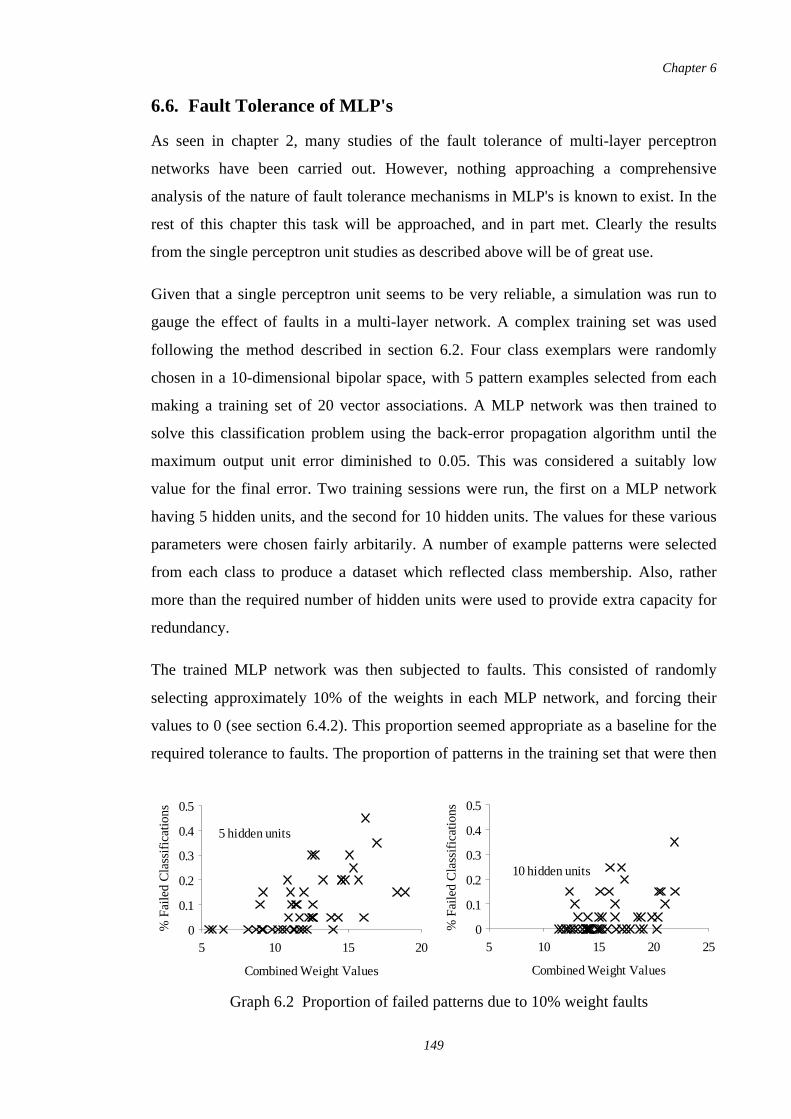
6.6. Fault Tolerance of MLP's
As seen in chapter 2, many studies of the fault tolerance of multi-layer perceptron
networks have been carried out. However, nothing approaching a comprehensive
analysis of the nature of fault tolerance mechanisms in MLP's is known to exist. In the
rest of this chapter this task will be approached, and in part met. Clearly the results
from the single perceptron unit studies as described above will be of great use.
Given that a single perceptron unit seems to be very reliable, a simulation was run to
gauge the effect of faults in a multi-layer network. A complex training set was used
following the method described in section 6.2. Four class exemplars were randomly
chosen in a 10-dimensional bipolar space, with 5 pattern examples selected from each
making a training set of 20 vector associations. A MLP network was then trained to
solve this classification problem using the back-error propagation algorithm until the
maximum output unit error diminished to 0.05. This was considered a suitably low
value for the final error. Two training sessions were run, the first on a MLP network
having 5 hidden units, and the second for 10 hidden units. The values for these various
parameters were chosen fairly arbitarily. A number of example patterns were selected
from each class to produce a dataset which reflected class membership. Also, rather
more than the required number of hidden units were used to provide extra capacity for
redundancy.
The trained MLP network was then subjected to faults. This consisted of randomly
selecting approximately 10% of the weights in each MLP network, and forcing their
values to 0 (see section 6.4.2). This proportion seemed appropriate as a baseline for the
required tolerance to faults. The proportion of patterns in the training set that were then
Chapter 6
149
Combined Weight Values
% F
aile
d C
lass
ifica
tions
0
0.1
0.2
0.3
0.4
0.5
5 10 15 20
5 hidden units
Combined Weight Values
% F
aile
d C
lass
ifica
tions
0
0.1
0.2
0.3
0.4
0.5
5 10 15 20 25
10 hidden units
Graph 6.2 Proportion of failed patterns due to 10% weight faults
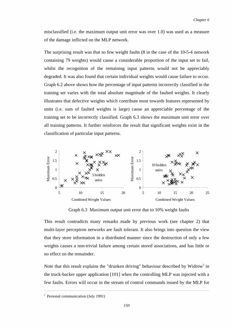
misclassified (i.e. the maximum output unit error was over 1.0) was used as a measure
of the damage inflicted on the MLP network.
The surprising result was that so few weight faults (8 in the case of the 10-5-4 network
containing 79 weights) would cause a considerable proportion of the input set to fail,
whilst the recognition of the remaining input patterns would not be appreciably
degraded. It was also found that certain individual weights would cause failure to occur.
Graph 6.2 above shows how the percentage of input patterns incorrectly classified in the
training set varies with the total absolute magnitude of the faulted weights. It clearly
illustrates that defective weights which contribute most towards features represented by
units (i.e. sum of faulted weights is large) cause an appreciable percentage of the
training set to be incorrectly classified. Graph 6.3 shows the maximum unit error over
all training patterns. It further reinforces the result that significant weights exist in the
classification of particular input patterns.
This result contradicts many remarks made by previous work (see chapter 2) that
multi-layer perceptron networks are fault tolerant. It also brings into question the view
that they store information in a distributed manner since the destruction of only a few
weights causes a non-trivial failure among certain stored associations, and has little or
no effect on the remainder.
Note that this result explains the "drunken driving" behaviour described by Widrow5 in
the truck-backer upper application [101] when the controlling MLP was injected with a
few faults. Errors will occur in the stream of control commands issued by the MLP for
5 Personal communication (July 1991)
Chapter 6
150
Combined Weight Values
Ma
xim
um
Err
or
0
0.5
1
1.5
2
5 10 15 20
5 hiddenunits
Combined Weight Values
Ma
xim
um
Err
or
0
0.5
1
1.5
2
5 10 15 20 25
10 hiddenunits
Graph 6.3 Maximum output unit error due to 10% weight faults
those inputs affected by the specific faults, and will cause the truck to turn in the wrong
direction. However, this causes it to move away from the particular region of input
space in which failure occurred, and so a correct output will eventually be generated
which turns the truck back on course. This sequence of events is repeated as the truck
reverses towards the loading bay. It would be interesting to study how many faults
would be tolerated before the overall behaviour of the truck is such that it does not
successfully align itself with the loading bay. Note that this is an example of the
problem noted in chapter 4 where the reliability of a neural network controlling a
dynamic system is not prejudiced by a single incorrect output, but by a sequence of
incorrect and correct outputs whose overall result combines to cause system failure.
6.6.1. Distribution of Information in MLP's
The traditional view of information distribution in neural networks, and multi-layer
perceptrons in particular, is by analogy to holographic storage; no single storage
element (normally taken to be a weight, or occasionally a unit) in a neural network
stores a particular pattern. Instead, patterns are stored in a distributed fashion across all
of the weights in a neural network. The conventional argument for fault tolerance is
that, as for a hologram, each weight in a neural network is unimportant globally, and so
its loss will not seriously impair the operation of the network. However, it is doubtful
whether this argument is valid for MLP's given the above results which showed that for
a small number of weight faults, a significant proportion of the training set is
misclassified. However, for a single perceptron unit it has been shown that a certain
number of weights can be viewed as being redundant in this fashion.
It is more appropriate for MLP networks to view each layer transforming patterns into a
different space, such that in the last hidden layer a representation is developed which is
linearly separable to produce the required output. This process can be viewed as
distributing the complex task of classification into several simpler steps at each hidden
layer. However, each layer of perceptron units can be viewed as being distributed in the
sense given in the previous paragraph. Reliability will arise from fault tolerance in each
layer of perceptron units, and overall will principally be governed by the least fault
tolerant layer.
Chapter 6
151
6.6.2. Analysis of Back-Error Propagation Learning
This section will consider why the back-error propagation algorithm does not produce a
MLP network configuration which exhibits the fault tolerant behaviour that might be
expected given the reliability of its individual perceptron units. This will be approached
by considering the effect of small changes in unit activation caused by weight faults. It
will then be shown that back-error propagation trained MLP networks are sensitive to
such changes.
The empirical results described above can be explained if the operation of a perceptron
unit is considered using the alternative visualisation described in section 6.3.3. The
projection of an input x onto its weight vector w' which suffers a fault in component f
can be described as follows
This scalar value s is now compared against the unit's bias θ to see if the degree by
which input x matches the feature w is sufficient to activate the unit. Looking at the
absolute difference between s and θ
It can be seen that the absolute difference between the fault-free projection and θ is
decreased, assuming every weight correctly contributes to the decision made by a
perceptron unit. If this value becomes negative, local failure will result since the unit
will then misclassify its input.
Although this describes the effect of a weight fault, it does not explain why only a few
faults generally cause such a dramatic failure in a multi-layer perceptron network for
some subset of the training set. It will now be shown how the back-error propagation
algorithm used to train the MLP network causes this lack tolerance to faults. The
common multiplicative term in the weight update ∆wij= ηδioj (equation 6.6) is
s= w ⋅ x = Σi=1
n
wixi − wfxf
w ⋅ x− θ = Σi=1
n
wixi − wfxf − θ
= Σi=1
n
wixi − θ − wfxf
= w ⋅ x −θ −wfxf
(6.9)
f i Σk wikok
⋅ oj = fi Σk wikok
⋅ fj Σl
wjl ol
(6.10)
Chapter 6
152
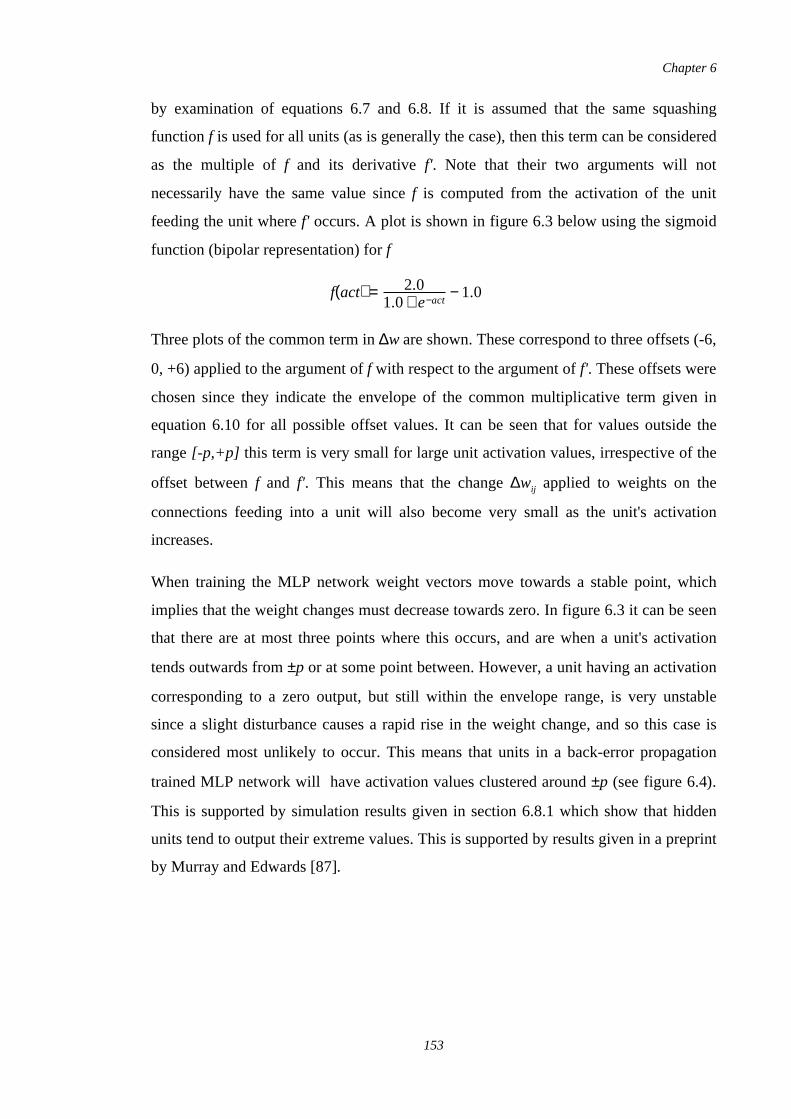
by examination of equations 6.7 and 6.8. If it is assumed that the same squashing
function f is used for all units (as is generally the case), then this term can be considered
as the multiple of f and its derivative f'. Note that their two arguments will not
necessarily have the same value since f is computed from the activation of the unit
feeding the unit where f' occurs. A plot is shown in figure 6.3 below using the sigmoid
function (bipolar representation) for f
Three plots of the common term in ∆w are shown. These correspond to three offsets (-6,
0, +6) applied to the argument of f with respect to the argument of f'. These offsets were
chosen since they indicate the envelope of the common multiplicative term given in
equation 6.10 for all possible offset values. It can be seen that for values outside the
range [-p,+p] this term is very small for large unit activation values, irrespective of the
offset between f and f'. This means that the change ∆wij applied to weights on the
connections feeding into a unit will also become very small as the unit's activation
increases.
When training the MLP network weight vectors move towards a stable point, which
implies that the weight changes must decrease towards zero. In figure 6.3 it can be seen
that there are at most three points where this occurs, and are when a unit's activation
tends outwards from ±p or at some point between. However, a unit having an activation
corresponding to a zero output, but still within the envelope range, is very unstable
since a slight disturbance causes a rapid rise in the weight change, and so this case is
considered most unlikely to occur. This means that units in a back-error propagation
trained MLP network will have activation values clustered around ±p (see figure 6.4).
This is supported by simulation results given in section 6.8.1 which show that hidden
units tend to output their extreme values. This is supported by results given in a preprint
by Murray and Edwards [87].
f(act) = 2.01.0+ e−act
− 1.0
Chapter 6
153
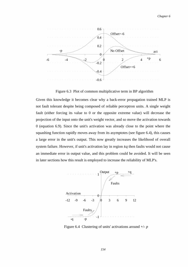
Given this knowledge it becomes clear why a back-error propagation trained MLP is
not fault tolerant despite being composed of reliable perceptron units. A single weight
fault (either forcing its value to 0 or the opposite extreme value) will decrease the
projection of the input onto the unit's weight vector, and so move the activation towards
0 (equation 6.9). Since the unit's activation was already close to the point where the
squashing function rapidly moves away from its asymptotes (see figure 6.4), this causes
a large error in the unit's output. This now greatly increases the likelihood of overall
system failure. However, if unit's activation lay in region ±q then faults would not cause
an immediate error in output value, and this problem could be avoided. It will be seen
in later sections how this result is employed to increase the reliability of MLP's.
-0.6
-0.4
-0.2
0
0.2
0.4
0.6
-6 -4 -2 0 2 4 6
act
+p
-p
Offset=-6
No Offset
Offset=+6
Figure 6.3 Plot of common multiplicative term in BP algorithm
-1
0
1
-12 -9 -6 -3 0 3 6 9 12
Activation
Output +p
-p
Faults
Faults
-q
+q
Figure 6.4 Clustering of units' activations around +/- p
Chapter 6
154

6.7. Training for Fault Tolerance
Various studies were undertaken into producing a technique which produced a fault
tolerant neural network based on the MLP. This work was motivated given that a MLP
trained using back-error propagation is not as fault tolerant as might have been
concluded from the results obtained in section 6.3 examining the reliability of a single
perceptron unit. The techniques included:
Limited interconnectivity
Local feedback at hidden and/or output layers
Training with weight faults injected
However, only the technique of injecting weight faults during training produced clear
results with respect to developing a MLP network which exhibits resilience to faults.
6.7.1. Training with Weight Faults
This method is similar to that used by Clay and Sequin which produces a fault tolerant
MLP network by injecting transient unit faults during training [71]. However, in section
6.4.2 it was shown that the basic functional entities in a MLP network which should be
considered are the weights on connections between units rather than the actual units.
Hence, weights were randomly set to 0 during training so that tolerance to weight faults
would be introduced. Work described by Murray and Edwards in a paper submitted for
publication [87] also uses this technique, though it concentrates on synaptic weight
noise rather than weight elimination. A training session consists of the following steps:
1. Randomly choose a fixed number of weights and fail them.
2. Apply back-error propagation algorithm for all patterns in training set.
3. Restore faulted weights and repeat from step 1 until the maximum output
unit error diminishes to an acceptable value.
Generally only a single weight was faulted during each training step, though
simulations were also carried out faulting multiple weights. However, the increase in
possible faulted weight combinations increases combinatorily, and so training rapidly
becomes prohibitively expensive.
Chapter 6
155
6.7.2. Comparison with Clay and Sequin's Technique
Superficially, there seems little difference between injecting weight faults during
training as against units being faulted. However, the argument for training with faults is
to imbue a neural network with resistance to those particular faults. Since the
construction of a fault model for a MLP (section 6.4.2) showed that only weight faults
are important in a MLP system, then it seems more reasonable to train injecting weight
faults. Unit faults are too abstract and unlikely to be representative of the effect of
physical faults in an implemented MLP. Due to this, it is expected that training with
weight faults will lead to better overall reliability.
Note that the technique of injecting weight faults during back-error propagation training
as a fault tolerance mechanism for a MLP network is not the major work described in
this chapter. Instead, this chapter concentrates on analysing the MLP networks
produced by fault injection training given that the back-error propagation algorithm
inherently produces non-fault tolerant classification systems. The results of this
analysis, combined with the previous analysis of the tolerance to faults of a single
perceptron unit, is used to show how a fault tolerant MLP network can be constructed
after normal back-error propagation training. This is a great advantage since the
extremely long training times required when training with faults injected in each
learning cycle will not be needed.
6.8. Analysis of Trained MLP
MLP networks trained with transient fault injection have been demonstrated to form
fault tolerant systems [28,71], and several reasons proposed to explain why this should
be so. Similar reasoning can be applied for training with unit faults.
The first line of reasoning views the faulted MLP network during training as a
sub-network due to the loss of a unit/weight. These sub-networks are then individually
trained to solve the problem, and their individual solutions converge such that global
agreement between them is reached. Once fully trained, the loss of a single weight can
easily be tolerated, and tolerance to more than one weight is due to distribution over the
sub-networks.
Chapter 6
156
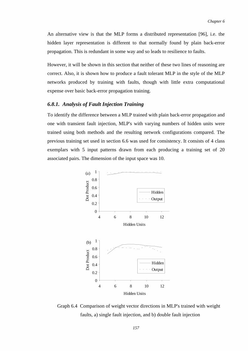
An alternative view is that the MLP forms a distributed representation [96], i.e. the
hidden layer representation is different to that normally found by plain back-error
propagation. This is redundant in some way and so leads to resilience to faults.
However, it will be shown in this section that neither of these two lines of reasoning are
correct. Also, it is shown how to produce a fault tolerant MLP in the style of the MLP
networks produced by training with faults, though with little extra computational
expense over basic back-error propagation training.
6.8.1. Analysis of Fault Injection Training
To identify the difference between a MLP trained with plain back-error propagation and
one with transient fault injection, MLP's with varying numbers of hidden units were
trained using both methods and the resulting network configurations compared. The
previous training set used in section 6.6 was used for consistency. It consists of 4 class
exemplars with 5 input patterns drawn from each producing a training set of 20
associated pairs. The dimension of the input space was 10.
Hidden Units
Do
t P
rod
uct
0
0.2
0.4
0.6
0.8
1
4 6 8 10 12
Hidden
Output
(a)
Hidden Units
Do
t P
rod
uct
0
0.2
0.4
0.6
0.8
1
4 6 8 10 12
Hidden
Output
(b)
Graph 6.4 Comparison of weight vector directions in MLP's trained with weight
faults, a) single fault injection, and b) double fault injection
Chapter 6
157
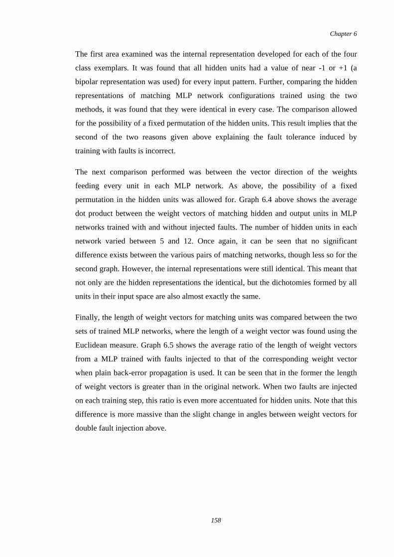
The first area examined was the internal representation developed for each of the four
class exemplars. It was found that all hidden units had a value of near -1 or +1 (a
bipolar representation was used) for every input pattern. Further, comparing the hidden
representations of matching MLP network configurations trained using the two
methods, it was found that they were identical in every case. The comparison allowed
for the possibility of a fixed permutation of the hidden units. This result implies that the
second of the two reasons given above explaining the fault tolerance induced by
training with faults is incorrect.
The next comparison performed was between the vector direction of the weights
feeding every unit in each MLP network. As above, the possibility of a fixed
permutation in the hidden units was allowed for. Graph 6.4 above shows the average
dot product between the weight vectors of matching hidden and output units in MLP
networks trained with and without injected faults. The number of hidden units in each
network varied between 5 and 12. Once again, it can be seen that no significant
difference exists between the various pairs of matching networks, though less so for the
second graph. However, the internal representations were still identical. This meant that
not only are the hidden representations the identical, but the dichotomies formed by all
units in their input space are also almost exactly the same.
Finally, the length of weight vectors for matching units was compared between the two
sets of trained MLP networks, where the length of a weight vector was found using the
Euclidean measure. Graph 6.5 shows the average ratio of the length of weight vectors
from a MLP trained with faults injected to that of the corresponding weight vector
when plain back-error propagation is used. It can be seen that in the former the length
of weight vectors is greater than in the original network. When two faults are injected
on each training step, this ratio is even more accentuated for hidden units. Note that this
difference is more massive than the slight change in angles between weight vectors for
double fault injection above.
Chapter 6
158
6.8.2. Comparison with MLP trained injecting unit faults
For comparison with the above results, simulations were also performed examining the
nature of MLP networks developed when training with unit faults injected. The
parameters of the simulation were similar in all other respects with its counterparts
above which analysed the weight vectors produced when training with weight faults.
Graph 6.6 below compares the MLP networks produced by training with a single
weight fault injected to those when a single unit fault is injected.
It can be seen that the direction of the weight vectors in both the hidden and output
layers of both MLP networks are almost identical. However, the length of weight
vectors in the MLP trained with unit faults injected are less than in the corresponding
MLP trained with weight faults. It will now be shown that this leads to a less fault
tolerant MLP network, as was expected in section 6.7.
Hidden Units
|We
igh
t| ra
tio1.2
1.3
1.4
1.5
1.6
1.7
1.8
4 6 8 10 12
Output
Hidden
(a)
Hidden Units
|Wei
ght|
Rat
io
0
1
2
3
4
5
6
4 6 8 10 12
Hidden
Output
(b)
Graph 6.5 Comparison of weight vector lengths in MLP's trained with weight
faults, a) single fault injection, and b) double fault injection
Chapter 6
159
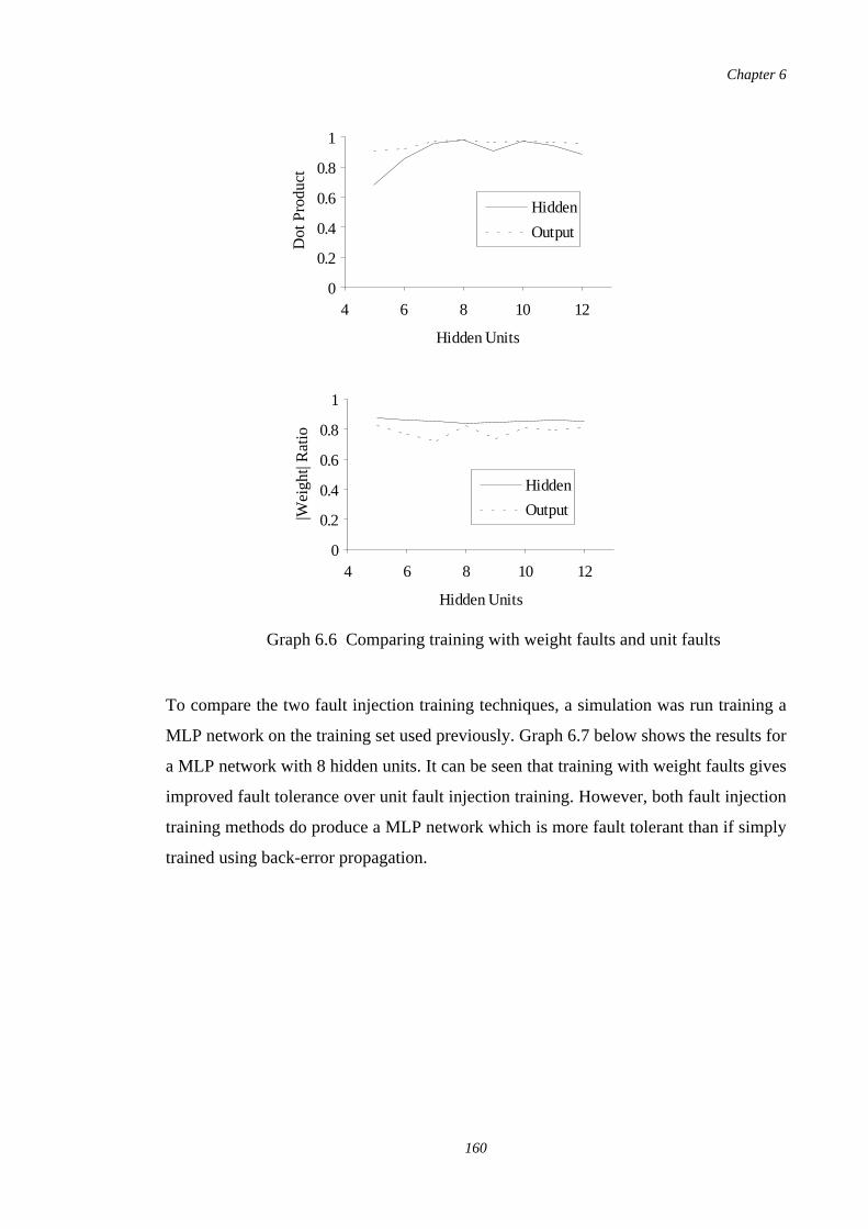
To compare the two fault injection training techniques, a simulation was run training a
MLP network on the training set used previously. Graph 6.7 below shows the results for
a MLP network with 8 hidden units. It can be seen that training with weight faults gives
improved fault tolerance over unit fault injection training. However, both fault injection
training methods do produce a MLP network which is more fault tolerant than if simply
trained using back-error propagation.
Hidden Units
Dot
Pro
duct
0
0.2
0.4
0.6
0.8
1
4 6 8 10 12
Hidden
Output
Hidden Units
|Wei
ght|
Rat
io
0
0.2
0.4
0.6
0.8
1
4 6 8 10 12
Hidden
Output
Graph 6.6 Comparing training with weight faults and unit faults
Chapter 6
160
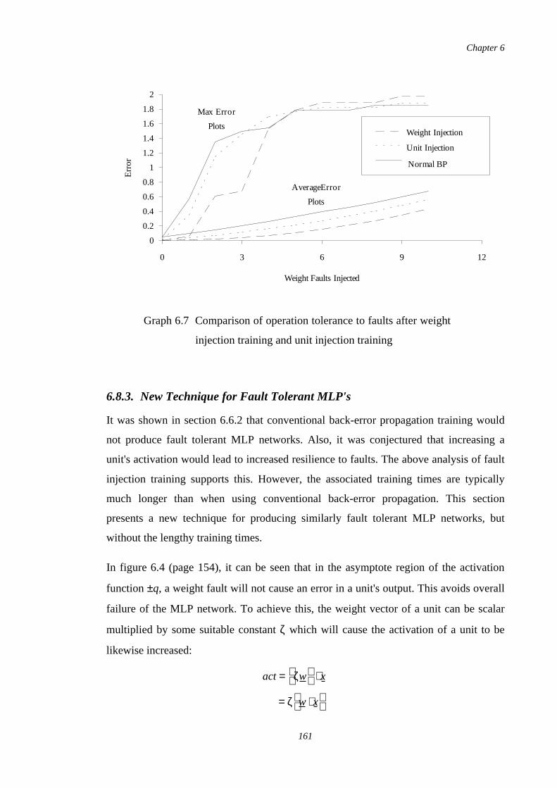
6.8.3. New Technique for Fault Tolerant MLP's
It was shown in section 6.6.2 that conventional back-error propagation training would
not produce fault tolerant MLP networks. Also, it was conjectured that increasing a
unit's activation would lead to increased resilience to faults. The above analysis of fault
injection training supports this. However, the associated training times are typically
much longer than when using conventional back-error propagation. This section
presents a new technique for producing similarly fault tolerant MLP networks, but
without the lengthy training times.
In figure 6.4 (page 154), it can be seen that in the asymptote region of the activation
function ±q, a weight fault will not cause an error in a unit's output. This avoids overall
failure of the MLP network. To achieve this, the weight vector of a unit can be scalar
multiplied by some suitable constant ζ which will cause the activation of a unit to be
likewise increased:
Weight Faults Injected
Err
or
0
0.2
0.4
0.6
0.8
1
1.2
1.4
1.6
1.8
2
0 3 6 9 12
AverageError
Plots
Max Error
Plots
Normal BP
Unit Injection
Weight Injection
Graph 6.7 Comparison of operation tolerance to faults after weight
injection training and unit injection training
act = ζw
⋅ x
= ζ w ⋅ x
Chapter 6
161
This will produce a unit which will tolerate a certain number of weight faults since the
output of the unit will not become erroneous, even though its absolute activation will
decrease. If every unit's weight vector is processed in this way, the entire MLP network
will tolerate a number of weight faults before failure occurs. This result is supported by
the previous analysis of MLP networks trained with faults injected in section 6.8.1
where it was found that the magnitude of weight vectors was greater than those in a
normal back-error propagation trained MLP network.
The feature of neural networks of indicating approaching failure due to graceful
degradation (c.f. section 3.7) will still be exhibited since as more weight faults affect a
unit, its absolute activation will decrease into the region where the squashing function
transits between output values. This will cause the output of the unit to become
increasingly erroneous, and so failure will not be a sudden discrete event.
Note that as , a unit will behave as if it were hard thresholded (c.f. section 6.3.1)ζ → ∞
and provides failure free service until the number of weight faults equals the Hamming
Distance between the centroids of its input classes6. However, at this point failure will
be abrupt since the change in activation caused by each weight fault will not be
mirrored by a gradual increase in the error of a unit's output as above. It can be seen
that a trade-off exists between the degree of graceful degradation required and the
degree of tolerance to faults, depending on the value ζ.
The enormous advantage of this technique to produce a fault tolerant MLP network
over that of fault injection training is that the training time is essentially only that
required for plain back-error propagation. This is a great improvement over the long
training times required to produce essentially the same MLP network configuration
when injecting faults during the training session.
Note that stretching a unit's weight vector is equivalent to sharpening its activation
function, i.e. compressing the activation region over which its output transitions
between asymptotic values. Sharpening an activation function is achieved by
multiplying the exponential term in the sigmoid function by a constant τ, which is often
6 Note that these input classes are not necessarily the training set classes. Also, the same assumptions
apply as in section 6.3.1.
Chapter 6
162
referred to as the temperature
If τ=ζ and the bias θ is incorporated into the weights, then
which shows the required equivalence.
6.9. Results of Scaled MLP Fault Tolerance
Simulations were performed to examine empirically the resilience to faults of MLP
networks with scaled weight vectors. The same training set as used in previous
simulations was used so that comparison with their results could be made. The number
of hidden units in the simulations ranged from 5 to 12. Note that the MLP networks
were trained using the normal back-error propagation algorithm. However, the final
weight vectors feeding into the hidden units were then scaled by a factor ζh, and
similarly ζo for output units to produce a fault tolerant MLP network.
To allow results from MLP networks with various numbers of hidden units to be
directly compared, the service degradation method (c.f. section 4.14.6) was used to
collect reliability data. This requires each fault to be assigned a constant failure rate λ,
which together with equation 6.11 below probabilistically models the occurrence of the
fault type at time t
The service degradation method implies that a simulation is started from time t0, and at
each time step the fault status of every weight is assessed according to equation 6.11.
The degree of failure of the MLP network is then measured by some means, and the
process repeated for the next time increment.
The measure of failure employed can either be discrete, or as is more appropriate for
neural networks (c.f. chapter 4), a continuous assessment of the system's reliability. The
measure used in these simulations was the proportion of inputs in the training set which
output = 1.0
1.0 +e−τ
w⋅x−θ
output = 1.0
1.0 + e−τ
w⋅x
= 1.0
1.0 +e−
ζw ⋅x
Pr fault occurs
= 1 −e−λt (6.11)
Chapter 6
163
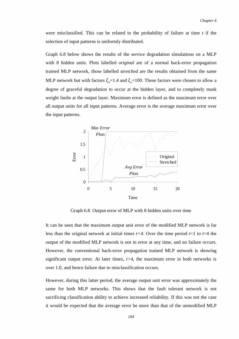
were misclassified. This can be related to the probability of failure at time t if the
selection of input patterns is uniformly distributed.
Graph 6.8 below shows the results of the service degradation simulations on a MLP
with 8 hidden units. Plots labelled original are of a normal back-error propagation
trained MLP network, those labelled stretched are the results obtained from the same
MLP network but with factors ζh=1.4 and ζo=100. These factors were chosen to allow a
degree of graceful degradation to occur at the hidden layer, and to completely mask
weight faults at the output layer. Maximum error is defined as the maximum error over
all output units for all input patterns. Average error is the average maximum error over
the input patterns.
It can be seen that the maximum output unit error of the modified MLP network is far
less than the original network at initial times t<4. Over the time period t=1 to t=4 the
output of the modified MLP network is not in error at any time, and no failure occurs.
However, the conventional back-error propagation trained MLP network is showing
significant output error. At later times, t>4, the maximum error in both networks is
over 1.0, and hence failure due to misclassification occurs.
However, during this latter period, the average output unit error was approximately the
same for both MLP networks. This shows that the fault tolerant network is not
sacrificing classification ability to achieve increased reliability. If this was not the case
it would be expected that the average error be more than that of the unmodified MLP
Time
Err
or
0
0.5
1
1.5
2
0 5 10 15 20
StretchedOriginal
Max Error
Plots
Avg Error
Plots
Graph 6.8 Output error of MLP with 8 hidden units over time
Chapter 6
164
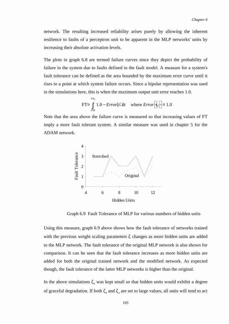
network. The resulting increased reliability arises purely by allowing the inherent
resilience to faults of a perceptron unit to be apparent in the MLP networks' units by
increasing their absolute activation levels.
The plots in graph 6.8 are termed failure curves since they depict the probability of
failure in the system due to faults defined in the fault model. A measure for a system's
fault tolerance can be defined as the area bounded by the maximum error curve until it
rises to a point at which system failure occurs. Since a bipolar representation was used
in the simulations here, this is when the maximum output unit error reaches 1.0.
Note that the area above the failure curve is measured so that increasing values of FT
imply a more fault tolerant system. A similar measure was used in chapter 5 for the
ADAM network.
Using this measure, graph 6.9 above shows how the fault tolerance of networks trained
with the previous weight scaling parameters ζ changes as more hidden units are added
to the MLP network. The fault tolerance of the original MLP network is also shown for
comparison. It can be seen that the fault tolerance increases as more hidden units are
added for both the original trained network and the modified network. As expected
though, the fault tolerance of the latter MLP networks is higher than the original.
In the above simulations ζh was kept small so that hidden units would exhibit a degree
of graceful degradation. If both ζh and ζo are set to large values, all units will tend to act
FT= ∫t=0
t=tf
1.0 −Error(t) dt where Error t f
= 1.0
Hidden Units
Fa
ult
To
lera
nce
0
1
2
3
4
4 6 8 10 12
Original
Stretched
Graph 6.9 Fault Tolerance of MLP for various numbers of hidden units
Chapter 6
165
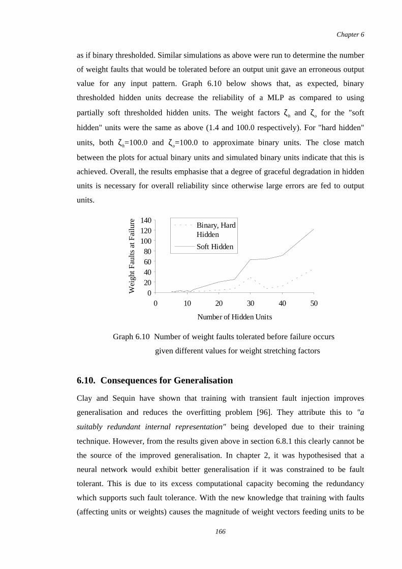
as if binary thresholded. Similar simulations as above were run to determine the number
of weight faults that would be tolerated before an output unit gave an erroneous output
value for any input pattern. Graph 6.10 below shows that, as expected, binary
thresholded hidden units decrease the reliability of a MLP as compared to using
partially soft thresholded hidden units. The weight factors ζh and ζo for the "soft
hidden" units were the same as above (1.4 and 100.0 respectively). For "hard hidden"
units, both ζh=100.0 and ζo=100.0 to approximate binary units. The close match
between the plots for actual binary units and simulated binary units indicate that this is
achieved. Overall, the results emphasise that a degree of graceful degradation in hidden
units is necessary for overall reliability since otherwise large errors are fed to output
units.
6.10. Consequences for Generalisation
Clay and Sequin have shown that training with transient fault injection improves
generalisation and reduces the overfitting problem [96]. They attribute this to "a
suitably redundant internal representation" being developed due to their training
technique. However, from the results given above in section 6.8.1 this clearly cannot be
the source of the improved generalisation. In chapter 2, it was hypothesised that a
neural network would exhibit better generalisation if it was constrained to be fault
tolerant. This is due to its excess computational capacity becoming the redundancy
which supports such fault tolerance. With the new knowledge that training with faults
(affecting units or weights) causes the magnitude of weight vectors feeding units to be
Number of Hidden Units
Wei
ght F
aults
at F
ailu
re
020406080
100120140
0 10 20 30 40 50
Binary, HardHidden
Soft Hidden
Graph 6.10 Number of weight faults tolerated before failure occurs
given different values for weight stretching factors
Chapter 6
166
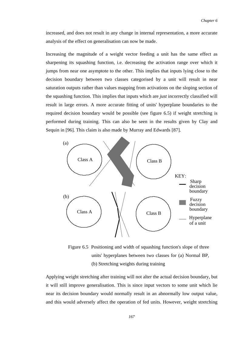
increased, and does not result in any change in internal representation, a more accurate
analysis of the effect on generalisation can now be made.
Increasing the magnitude of a weight vector feeding a unit has the same effect as
sharpening its squashing function, i.e. decreasing the activation range over which it
jumps from near one asymptote to the other. This implies that inputs lying close to the
decision boundary between two classes categorised by a unit will result in near
saturation outputs rather than values mapping from activations on the sloping section of
the squashing function. This implies that inputs which are just incorrectly classified will
result in large errors. A more accurate fitting of units' hyperplane boundaries to the
required decision boundary would be possible (see figure 6.5) if weight stretching is
performed during training. This can also be seen in the results given by Clay and
Sequin in [96]. This claim is also made by Murray and Edwards [87].
Applying weight stretching after training will not alter the actual decision boundary, but
it will still improve generalisation. This is since input vectors to some unit which lie
near its decision boundary would normally result in an abnormally low output value,
and this would adversely affect the operation of fed units. However, weight stretching
Class A
Class A
Class B
Class B
decision
decision
boundary
boundary
Hyperplane
KEY:
(a)
(b)
of a unit
Sharp
Fuzzy
Figure 6.5 Positioning and width of squashing function's slope of three
units' hyperplanes between two classes for (a) Normal BP,
(b) Stretching weights during training
Chapter 6
167
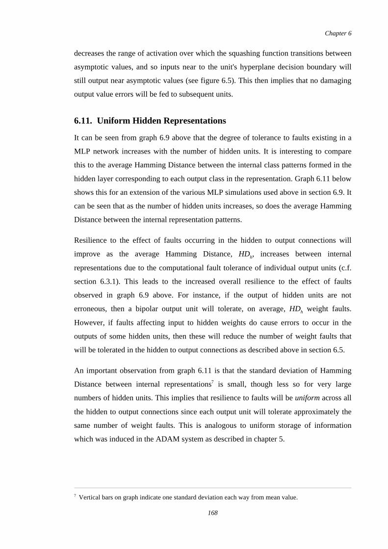
decreases the range of activation over which the squashing function transitions between
asymptotic values, and so inputs near to the unit's hyperplane decision boundary will
still output near asymptotic values (see figure 6.5). This then implies that no damaging
output value errors will be fed to subsequent units.
6.11. Uniform Hidden Representations
It can be seen from graph 6.9 above that the degree of tolerance to faults existing in a
MLP network increases with the number of hidden units. It is interesting to compare
this to the average Hamming Distance between the internal class patterns formed in the
hidden layer corresponding to each output class in the representation. Graph 6.11 below
shows this for an extension of the various MLP simulations used above in section 6.9. It
can be seen that as the number of hidden units increases, so does the average Hamming
Distance between the internal representation patterns.
Resilience to the effect of faults occurring in the hidden to output connections will
improve as the average Hamming Distance, HDh, increases between internal
representations due to the computational fault tolerance of individual output units (c.f.
section 6.3.1). This leads to the increased overall resilience to the effect of faults
observed in graph 6.9 above. For instance, if the output of hidden units are not
erroneous, then a bipolar output unit will tolerate, on average, HDh weight faults.
However, if faults affecting input to hidden weights do cause errors to occur in the
outputs of some hidden units, then these will reduce the number of weight faults that
will be tolerated in the hidden to output connections as described above in section 6.5.
An important observation from graph 6.11 is that the standard deviation of Hamming
Distance between internal representations7 is small, though less so for very large
numbers of hidden units. This implies that resilience to faults will be uniform across all
the hidden to output connections since each output unit will tolerate approximately the
same number of weight faults. This is analogous to uniform storage of information
which was induced in the ADAM system as described in chapter 5.
7 Vertical bars on graph indicate one standard deviation each way from mean value.
Chapter 6
168
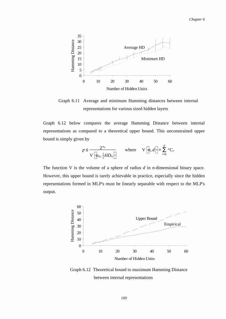
Graph 6.12 below compares the average Hamming Distance between internal
representations as compared to a theoretical upper bound. This unconstrained upper
bound is simply given by
The function V is the volume of a sphere of radius d in n-dimensional binary space.
However, this upper bound is rarely achievable in practice, especially since the hidden
representations formed in MLP's must be linearly separable with respect to the MLP's
output.
Number of Hidden Units
Ham
min
g D
ista
nce
05
101520253035
0 10 20 30 40 50 60
Minimum HD
Average HD
Graph 6.11 Average and minimum Hamming distances between internal
representations for various sized hidden layers
p ≤ 2nh
V nh, 1
2HDh
where V n,d
= Σr=0
dnCr
Number of Hidden Units
Ham
min
g D
ista
nce
0
10
20
30
40
50
60
0 10 20 30 40 50 60
EmpiricalUpper Bound
Graph 6.12 Theoretical bound to maximum Hamming Distance
between internal representations
Chapter 6
169
It can be seen from graph 6.12 that the average Hamming Distance between internal
representations formed by back-error propagation training in MLP's diverges from the
theoretical maximum as more hidden units are used. It may be possible that better
internal representations with increased class separation could be formed during training
which will lead to increased tolerance to faults. If this could be achieved, the reliability
of a MLP network would be further improved.
6.12. Conclusions
This chapter has analysed the fault tolerance of perceptron units, and concluded that
individually they are extremely reliable. However, it was found that a MLP network
was not as fault tolerant as might be expected given this result. It has shown that
training with weight faults develops a fault tolerant multi-layer perceptron network in a
similar fashion as injecting unit faults described in [71]. The trained fault tolerant MLP
networks were extensively analysed to locate the mechanism which lead to their
robustness. It was found that the both the hidden representations and the directions of
weights vectors were not significantly different to a MLP network trained with normal
back-error propagation. The only discrepancy was in the magnitude of the weight
vectors.
Separate analysis of the effect of faults in a MLP, and the activation of units in a trained
MLP, showed how the back-error propagation algorithm results in individual units not
being fault tolerant due to insufficient unit activation levels. It was then shown that by
scalar multiplying every weight vector by factor ζ, each unit in the MLP would then be
capable of exhibiting fault tolerance as suggested by the initial analysis of a single
perceptron unit. This leads to better overall tolerance to faults in the entire MLP. An
advantage of this new technique as opposed to training with transient fault injection is
that training times are much reduced. Simulations were carried out which showed that
these two methods give comparable results, as would be expected.
An analysis of the hidden representations formed by back-error propagation training
showed that with more hidden units, the average Hamming Distance between internal
representations in the hidden layer of a MLP increases. As expected from the analysis
of the perceptron unit, it was found that the increased class separation lead to improved
tolerance to the effect of faults in the entire MLP. This was then verified by the results
Chapter 6
170
from various simulations. Further, the small standard deviation in the Hamming
Distance between internal representations implied that the effect of faults would be
approximately uniform across the hidden to output connections. This can be compared
to the uniform storage technique developed in chapter 5 for the ADAM network.
In conclusion, this chapter has shown how to allow a MLP network to use the inherent
fault tolerance its perceptron-like units to produce an overall fault tolerant system. As
discussed in section 6.6.1, this is only one area of distributed processing which results
in fault tolerance being exhibited by a MLP. The other is to force the development of
redundant representations in each hidden layer. Although the simulations above showed
that as more hidden units are added to a MLP the Hamming Distance between internal
representations increases, and hence also resilience to faults, it is unlikely that the
maximum fault tolerance possible is achieved.
Chapter 6
171
CHAPTER SEVEN
Conclusions
7.1. Overview
This thesis has examined the effect of faults on the reliability of the operation of
artificial neural networks. Their functionality was visualised at an abstract level rather
than considering actual implementations so that the fault tolerance arising from their
computational nature could be analysed. It also allowed the question to be posed "do
neural networks possess inherent fault tolerance?". Other reasons for making this
decision are given in chapter 3. Various concepts relating to techniques for achieving
fault tolerance in neural networks were also discussed in this chapter. These included
distribution of information and processing, generalisation, and the architectural
structure of neural networks. It was also considered whether requiring fault tolerant
behaviour could be applied as a constraint in a neural network to improve its
generalisation. The style of failure in neural networks was studied with respect to the
type of problems for which their computational nature is most suited, and the reasons
for neural networks exhibiting graceful degradation analysed.
A methodology was defined in chapter 4 by which the effect of fault tolerance
techniques on a neural network's reliability could be assessed. It addressed issues such
as the construction of fault models for systems visualised at an abstract level,
approaches to measuring the effect of faults on a system's reliability, and also various
simulation frameworks. In appendix A, it was shown how this methodology can be
applied to assess the reliability of a feedback neural network based only on a high-level
functional specification of its operation. This provided a very general approach to
reliability assessment in cases where no error function is provided by the learning
algorithm.
Chapter 7
172
Using this methodology, various neural network models were then investigated to gain
an understanding of the effect of faults on their operation. This knowledge identified
various potentials for inherent fault tolerance in neural networks, and lead to techniques
being developed to improve reliability by increasing resilience to the effect of faults.
These results will be summarised in this chapter.
7.2. Basis for Inherent Fault Tolerance
The simple perceptron unit which is used in various forms in many neural network
models has been shown to be highly fault tolerant. It was shown in chapter 6 that the
number of weight faults can be tolerated before failing to distinguish between two
classes is dependant on the Hamming Distance (HD) between them. Another factor is
whether it operates on bipolar or binary inputs. It was shown that the maximum number
of weights which can be defective in the case of a bipolar perceptron unit is HD, while
only for a binary unit.12HD
This basic result implies that neural networks employing perceptron-like units can be
made fault tolerant by ensuring that the characteristics of the input domain1 to a unit
meet the above requirements.
7.3. Fault Tolerance Mechanisms
This section will combine the various results from investigations in to ADAM in
chapter 5 and MLP's in chapter 6. The various computational properties in artificial
neural networks that lead to resilience to faults on their operation will be summarised.
These include ensuring uniform distribution, modular redundancy, architectural
constructs, and learning algorithms.
7.3.1. Uniform Fault Tolerance
A major factor in neural computation which leads to fault tolerant behaviour is that of
uniform distribution of information. By this it is meant that in addition to information
being distributed throughout a neural network's components during training, the
functional load placed on each component is approximately equal. Uniform distribution
implies that the effect of faults is not limited to a particular a region of input space.
1 Note that this is not necessarily the input domain to the neural network. The input domain to an output
unit in a MLP comes from the hidden layer.
Chapter 7
173
Instead faults cause degradation to the neural network's operation over a wide range of
inputs. This can be viewed as providing uniform fault tolerance. It was noted in chapter
3 that this characteristic would not occur in neural networks exhibiting local
generalisation, and so only globally generalising neural networks were studied in this
thesis.
In ADAM it was found that by ensuring all rows in the associative storage matrix
would store an equal number of class vectors on average, a great improvement in
resilience to faults could be achieved. This uniform storage was accomplished by the
addition of an extra preprocessing stage to ADAM which incurs very little extra
computational cost. Although the technique implies that twice the number of resources
are required, it was shown that the benefits with respect to increased reliability
outweighed these costs.
A similar result was found for the multi-layer perceptron network. The internal
representations formed by training with a modified back-error propagation algorithm in
MLP's with various numbers of hidden units were examined. It was found that the
average Hamming Distance between the hidden representations formed for each class
centre was proportional to the number of hidden units. More importantly, the standard
deviation was small in comparison which implies uniform storage occurs. This can be
explained by considering that, as described above, the fault tolerance of an unit in a
MLP is dependant upon the Hamming Distance between its input classes. Since all
hidden representations are approximately equidistant in terms of Hamming Distance,
this implies that output unit's resilience to faults will be near uniform.
7.3.2. Modular Redundancy
A more well known fault tolerance mechanism for achieving increased reliability has
been examined for the ADAM network, and also indirectly for the MLP network.
Redundancy can be achieved by replicating sub-systems, and so improve reliability if
the increased complexity of the overall system does not prejudice this. In ADAM, the
basic system module is a tuple unit together with the matrix region which it addresses.
Its output consists of the required class vector plus noise due to some level of memory
saturation.
Chapter 7
174
It was shown that increasing the number of tuple modules improved the overall
reliability of the system without being compromised by too rapid a rise in complexity.
This analysis was achieved by modelling the occurrence of faults using a time-based
probability density function which allows varying sized systems to be compared
realistically, as was described in chapter 3.
In MLP networks, the hidden unit can be viewed as the basic functional entity
controlling the capacity of the overall system. As with ADAM, it was shown that
employing more hidden units increases overall reliability even with the resulting
heightened system complexity.
7.3.3. Architectural Considerations in ADAM
The function of specific functional components in some neural network models may
have bearing on the overall system if they occur in sufficient numbers and have a
significant role. In ADAM, such a component is the tuple unit. These comprise the
preprocessing layer which forms the vector input to the associative matrix. Their
function and number require that their reliability must be taken into account. Results
given in chapter 5 showed that small tuple units should be used in ADAM systems for
greatest reliability. This is due to their lower potential noise levels in the presence of
faults (activating extra matrix rows).
This result reinforces the conclusions given for modular redundancy above where using
many tuple units increases ADAM's reliability in the presence of faults. This is since the
dimensions of a problem's input space specifies the dimensions of ADAM, and a small
tuple size implies that a large number of tuple units will be required.
Another objective in assessing computational fault tolerance is that of locating potential
critical faults. These are important to identify since it allows future implementation
designs to specifically protect against them. Fault injection experiments in ADAM
indicated that stuck-at-1 faults in the key vector and stuck-at-0 matrix link faults have
the greatest effect on its reliability.
7.3.4. Learning in Multi-Layer Perceptron Networks
It was found that a few critical weights will exist in MLP's trained using the back-error
propagation learning algorithm. This was surprising since perceptron-like units which
Chapter 7
175
are the basic building blocks of MLP's can be fault tolerant (section 7.2). Due to this
result a training method which develops fault tolerant MLP's was then examined. The
MLP is trained using the normal back-error propagation algorithm, but small numbers
of transient faults are injected at each step. This results in a MLP which tolerates many
faults, though the training time can be very long.
First, a more appropriate fault model than those which other researchers have used for
the MLP network was developed using the methodology described in chapter 3. Rather
than considering unit faults, weights were identified as the basic defect. Transient fault
injection training was then performed, and it was found that the MLP's exhibited better
fault tolerance than when unit faults are injected during training.
These fault tolerant MLP's were then analysed to determine the source of their
increased reliability. It was found that both the internal representations formed and the
direction of the units' weight vectors were essentially unchanged. The only difference
observed was that the magnitude of the weight vectors was greatly increased. The
mechanism by which this change lead to increased reliability was discovered by
considering the effect of faults on a unit's activation. It was shown that a weight fault
causes the absolute activation to decrease. If weights are small, then a loss of unit
activation causes the absolute output of a unit to decrease in the region where the
thresholding function transits between its two output extremes. By increasing the
magnitude of weights the average activation of units lies further away from this region
of the thresholding function. This results in faults not causing an immediate decrease in
a unit's output. It was also shown that this is functionally equivalent to sharpening a
unit's thresholding function. This technique is another fault tolerance mechanism for
perceptron-like units (c.f. section 7.2). To summarise, this mechanism decreases the
sensitivity of a unit's output to changes in its activation caused by faults.
The back-error propagation learning algorithm was then analysed to discover why it
produced weight configurations resulting in such limited unit activation. This involved
studying the dominant terms in the weight change equations. It was shown that units'
activations will be limited in magnitude to values clustering around the region where
the thresholding function begins to approach its asymptotes. This lead to the lack of
resilience to the effect of faults as described above.
Chapter 7
176
An extremely useful result from this analysis was that a fault tolerant MLP, similar to
one trained with transient fault injection, can be constructed merely by the scalar
multiplication of weight vectors after training with basic back-error propagation. This
precludes the extremely long learning times required when transient fault injection
training is employed. It was also shown that a similar result can be obtained by merely
sharpening the thresholding functions in each unit.
In section 7.2, another fault tolerance mechanism was described which was found to
result in increased reliability in a perceptron unit depending on the Hamming Distance
between the two classes which it distinguishes. To assess this, MLP's with varying
numbers of hidden units in their intermediate layer were trained on a fixed classification
problem. As expected, reliability increased with the number of hidden units used. The
Hamming Distance between the internal representations formed for each input class
were then measured. It was found that the standard deviation of internal representations
was low implying that they were fairly uniformly distributed in Hamming space (c.f.
section 7.3.1). Also, it was shown that the average Hamming Distance was close to a
theoretical upper bound implying that the back-error propagation algorithm does
develop internal representations which will lead to fault tolerance in this respect.
7.4. Inherent Fault Tolerance?
In conclusion, results given in this thesis have shown that neural networks do have the
potential to be inherently fault tolerant, although current learning algorithms do not
always develop appropriate weight configurations. For example, it was shown how the
activation of units in a MLP trained using back-error propagation algorithm lie at a
critical point on the thresholding function, and faults cause their absolute output to
decrease. In ADAM, class vectors are not stored in a uniform manner in the associative
matrix, and localised memory saturation occurs.
It was noted in chapter 2 that the question of whether neural networks are inherently
fault tolerant is currently undecided in the literature. This conflict has been shown to
arise due to a distinction not being made between considering the neural computational
paradigm and trained neural networks. Given their implicit assumptions, both views are
essentially correct. Neural networks do have the potential to be inherently fault tolerant
given a suitable learning algorithm. However, current algorithms such as back-error
Chapter 7
177
propagation do not develop suitable weight configurations. To achieve fault tolerance in
the one layer binary weighted neural networks in ADAM, the loss of information
during training when new links have already been previously set must be minimised.
7.5. Implications for Future Research
The research presented in this thesis has shown that inherent fault tolerance mechanisms
do exist in neural networks, and various constructive techniques have been developed
which promote these. However, the research has also indicated various avenues which
seem promising for future research.
7.5.1. Generalisation
In chapter 3 it was proposed that applying fault tolerance as a constraint during learning
will improve generalisation in neural networks. This thesis has not examined this area
in any detail, instead it has concentrated on the initial problem of developing fault
tolerance mechanisms. However, it would be useful to determine if this proposal has
any justification. Generalisation in the presence of input noise seems likely if the
distortion caused by faults is functionally similar. In particular, the effect of uniform
distribution of information, which has been shown to be a fault tolerance mechanism,
on generalisation deserves examination. For instance, maximising distance between
internal representations in MLP's could result in decreasing generalising if too diverse
representations are formed.
The area of computational learning theory (CLT) could also be used to examine
rigourously the effects of imposing fault tolerance as a constraint in neural networks.
This mathematical framework addresses the question of whether a general learning
device will correctly generalise, i.e. learn to represent the underlying problem. A central
equation in CLT considers the number of training examples that are required to
constrain a model with some given capacity. Recognising that improving fault tolerance
reduces the capacity of a system, the number of training examples required will be
reduced. Lines of work would be to develop bounds on the capacity of a neural network
when certain fault tolerance mechanisms are imposed.
Chapter 7
178
7.5.2. Internal Representations
This also suggests another line of research. Current bounds on the theoretical maximum
Hamming Distance between internal representations could be improved. For example,
the constraint that each class must be linearly separable from the other classes
corresponding to internal representations could be introduced. This will allow the
effectiveness of learning algorithms, such as back-error propagation, to be assessed in
neural networks composed of perceptron-like units with respect to the resilience of
individual units to faults.
7.5.3. Implementations
Another important area is to consider how computational fault tolerance mechanisms as
described in this thesis can be preserved in an implementation design. This will allow
inherent fault tolerance to be achieved at little or no extra complexity. Also, the effect
of conventional fault tolerance techniques applied at the implementation level to further
enhance reliability should be assessed. However, an objective should be that the fault
tolerance due to a neural network's computational nature is not compromised, and this
provides another area which can be examined.
7.5.4. Neural Fault Tolerance
Finally, additional fault tolerance mechanisms should be sought at the computational
level in artificial neural networks. In particular, neural network models involving forms
of feedback should be considered. The question of whether errors caused by transient
faults can be self-corrected in an iterative neural network is of great interest, especially
when applied to control problems.
Certainly this final section does not cover all areas connected with fault tolerance
mechanisms and reliability deserving future research, but it can be seen that there is a
large scope for study.
Chapter 7
179
APPENDIX A
Fault Tolerance of Lateral
Interaction Networks
This appendix was a paper published in IJCNN-91, Singapore [109]. It is included in
this thesis as an example of how the degree of failure in an artificial neural network can
be assessed from a specification of its functionality, rather than by using a test set of
data (c.f. chapter 4).
A.1. Introduction
Neural networks offer a parallel distributed method of processing information unlike
that of conventional serial computing systems, also their underlying basis of
computation is analogue rather than digital. Although they were inspired from studies
of the structure of the brain [62], artificial neural networks are a very simplified model
of biological neural networks, and are also very much smaller. However, it is generally
accepted that neural networks are well suited to solve problems which are very
successfully tackled by biological neural systems such as our brain.
Artificial neural networks consist of a large number of simple processing units (often
termed neurons) which are highly interconnected. Each unit forms a weighted sum of
its inputs, then thresholds it with respect to some internal bias value using some
bounded non-linear function. The selection of suitable weights and biases such that a
problem is solved is performed by some (normally iterative) algorithm; this process has
been termed learning.
It has commonly been mentioned that neural networks are naturally fault tolerant
[7,8,13,22], i.e. will continue to provide acceptable service in the presence of faults.
The intuitive reasoning behind this assertion is that their distributed processing is
Appendix A
180
resilient to errors caused by faults, and large fan-in to individual units renders
insignificant the effect that faults can cause.
The objective of this paper is to examine the fault tolerance of lateral inhibition arrays.
Section A.2 discusses the suitability of applying neural networks to application areas
with respect to their solution characteristics. The structure and operation of lateral
inhibition arrays is then described in section A.3. Section A.4 defines a fault model.
Failure is considered in section A.5, and it is discussed how its occurrence depends
upon the lateral inhibition array's application area. Section A.6 details the empirical
results obtained. Finally conclusions are drawn.
A.2. Soft/Rigid Application Areas
Application area solutions can be identified as either soft or rigid. Considering the
solution of a problem to be represented by a function from some N-dimensional space
to M-dimensional space, then it can be termed soft if the function is fairly smooth and
continuous, i.e. as an input vector traverses its space, the output vector will also do
likewise.
Conversely, a rigid problem is characterised by a discrete mapping, and an instance of
the problem has an clear-cut exact solution. It will generally be the case that solutions
given for various similar instances will not themselves be similar.
Most neural networks can either perform a functional mapping or classification
depending on whether the thresholding function applied to its output units is linear or
saturates/hard-limiting. The output of the former will span over the entire output space,
whilst the latter will always produce a restricted set of output vectors. The concept of
generalisation in neural networks should be distinguished between these two categories.
For a classification system, generalisation implies that input patterns close to a stored
pattern will be given the same class. For a neural network performing a functional
mapping though, generalisation will generally involve some form of interpolation.
Neural networks will exhibit generalisation when solving soft problems since regions
around input-output pairs are related rather than only the actual points, as is the case
with rigid problems.
If x → f x then x+ δx → f x
+ δx as δx → 0
Appendix A
181
Note that it may be possible in some cases to change the representation of the instance
of a problem such that a seemingly rigid problem may become soft. This will happen if
the new representation has the property of adjacency, i.e. nearby members of the
representation are nearby in problem space. For example, binary addition is rigid, but
by representing it using real numbers it becomes soft. This technique can be a key
element in helping to attain generalisation in neural network systems.
A.2.1. Implications for Reliability
Any system will inevitably be affected by factors such as noise and uncertainty for
example, and so any particular instance of a problem will actually be represented by a
small region in input space. However, if the problem is soft, then this will map to
another region in output space. This leads to noise tolerance, though it also implies that
the concept of a precise answer being produced by such a system is meaningless.
The inherent fault tolerance of neural networks can be reinforced given suitable
input-output representation and internal computational processing. High fan-in to units
means that although faults may cause severe local damage (e.g. weight set to opposite
extreme), this will only cause a deviation from fault-free unit output values. The
influence of a single input to a unit is limited. Even if a unit was faulty, the extreme
case of its output going to its opposite extreme would only cause a single input to all
subsequent units to be affected. So, if the input-output representation chosen is such
that the problem is soft, then this deviation from fault-free values will be tolerated due
to adjacency.
A.2.2. Verification
Neural network learning algorithms tend only to approach the optimum set of weights
and biases for a problem, i.e. it is possible that some problems cannot be perfectly
solved. This implies that even a fault-free neural network may not produce exactly the
desired response for any given input. If generalisation is relied upon, then the output
quality will be even more degraded. However, for soft problem domains where exact
solutions are not appropriate, this is acceptable behaviour, though verifying that a
neural network meets its specification will be very hard. For example, it could be that a
small portion of input space is not properly generalised, and that failure will occur if it
Appendix A
182
is accessed. This will not be detected with absolute certainty by testing, and exhaustive
testing is likely to be unfeasible.
Some neural networks paradigms (e.g. Kohonen [91], Barto et al [120]) incorporate the
idea of continual adaptation to both environment and/or internal structure. These
present a special problem for verification. It is possible that a system could adapt in
stages, each stage being built on a previously verified core, and then the new system
itself being verified.
A.3. Lateral Inhibition
Lateral inhibition arrays, also known as centre-on surround-off cells, are a class of
single-layer neural networks with feedback between output units. They developed from
studies of Limulus (the Horseshoe crab) by Hartline and Ratliff [121] where it was
found that lateral inhibitory feedback occurred between nearby receptor units in its
optical system. This can be generalised to include excitatory feedback as well, and in
general, the functional structure of such feedback to a particular neuron from
surrounding neurons depends on the distance between them. The central neuron is
excited by nearby neurons, a ring of neurons surrounding these exert an inhibitory
influence, whilst more distant neurons supply weak excitation. These can be termed
lateral interaction networks.
To simulate such a system, N units are arranged in a single layer, and connections are
made to each unit from neighbouring units. The value of the weight of each connection
is derived from a Mexican-hat function (see figure A.1). For simplicity only 1D-arrays
of units are considered in this paper, though it is expected that results can be generalised
to higher dimensions. Simulations used a more discrete form of the Mexican-hat
function ignoring the long-distant weak excitation. Note that units near the array edges
will be unduly influenced from the interior due to imbalance between their incoming
excitatory and inhibitory influences, and so various boundary effects will occur. Since
the size of arrays used in simulations are limited, these effects would cause noticeable
distortion. To overcome this, the array of units was joined together at its ends, thus
Appendix A
183
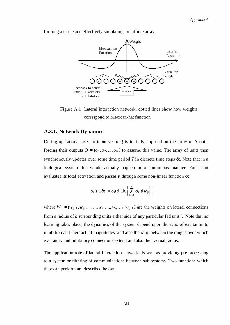
forming a circle and effectively simulating an infinite array.
Figure A.1 Lateral interaction network, dotted lines show how weights
correspond to Mexican-hat function
A.3.1. Network Dynamics
During operational use, an input vector I is initially imposed on the array of N units
forcing their outputs to assume this value. The array of units thenO = (o1,o2, ...,oN)
synchronously updates over some time period T in discrete time steps δt. Note that in a
biological system this would actually happen in a continuous manner. Each unit
evaluates its total activation and passes it through some non-linear function σ:
where are the weights on lateral connectionsWi = (wij−k,wij−k+1, ...,wi0, ...,wij+k−1,wij+k)
from a radius of k surrounding units either side of any particular fed unit i. Note that no
learning takes place; the dynamics of the system depend upon the ratio of excitation to
inhibition and their actual magnitudes, and also the ratio between the ranges over which
excitatory and inhibitory connections extend and also their actual radius.
The application role of lateral interaction networks is seen as providing pre-processing
to a system or filtering of communications between sub-systems. Two functions which
they can perform are described below.
Weight
LateralDistance
Input
Mexican-hatFunction
Feedback to centralunit: '+' Excitatory '-' Inhibitory
Value forweight
+ ++ - - - -----
oi(t +δt) = oi(t) + σ Σj=−k
k
oi(t)wij
Appendix A
184
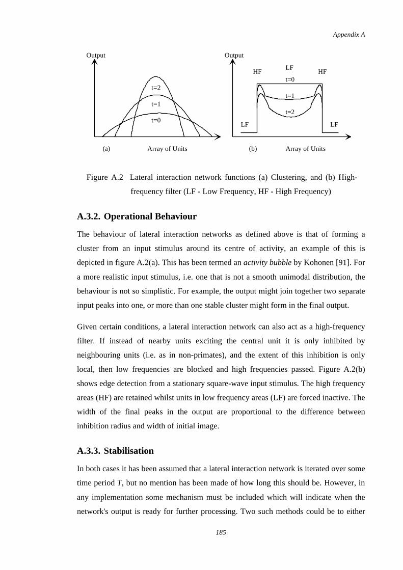
Figure A.2 Lateral interaction network functions (a) Clustering, and (b) High-
frequency filter (LF - Low Frequency, HF - High Frequency)
A.3.2. Operational Behaviour
The behaviour of lateral interaction networks as defined above is that of forming a
cluster from an input stimulus around its centre of activity, an example of this is
depicted in figure A.2(a). This has been termed an activity bubble by Kohonen [91]. For
a more realistic input stimulus, i.e. one that is not a smooth unimodal distribution, the
behaviour is not so simplistic. For example, the output might join together two separate
input peaks into one, or more than one stable cluster might form in the final output.
Given certain conditions, a lateral interaction network can also act as a high-frequency
filter. If instead of nearby units exciting the central unit it is only inhibited by
neighbouring units (i.e. as in non-primates), and the extent of this inhibition is only
local, then low frequencies are blocked and high frequencies passed. Figure A.2(b)
shows edge detection from a stationary square-wave input stimulus. The high frequency
areas (HF) are retained whilst units in low frequency areas (LF) are forced inactive. The
width of the final peaks in the output are proportional to the difference between
inhibition radius and width of initial image.
A.3.3. Stabilisation
In both cases it has been assumed that a lateral interaction network is iterated over some
time period T, but no mention has been made of how long this should be. However, in
any implementation some mechanism must be included which will indicate when the
network's output is ready for further processing. Two such methods could be to either
Output
Array of Units
t=0
t=1
t=2
Output
Array of Units(a) (b)
t=0
t=1
t=2
HFLF
HF
LFLF
Appendix A
185
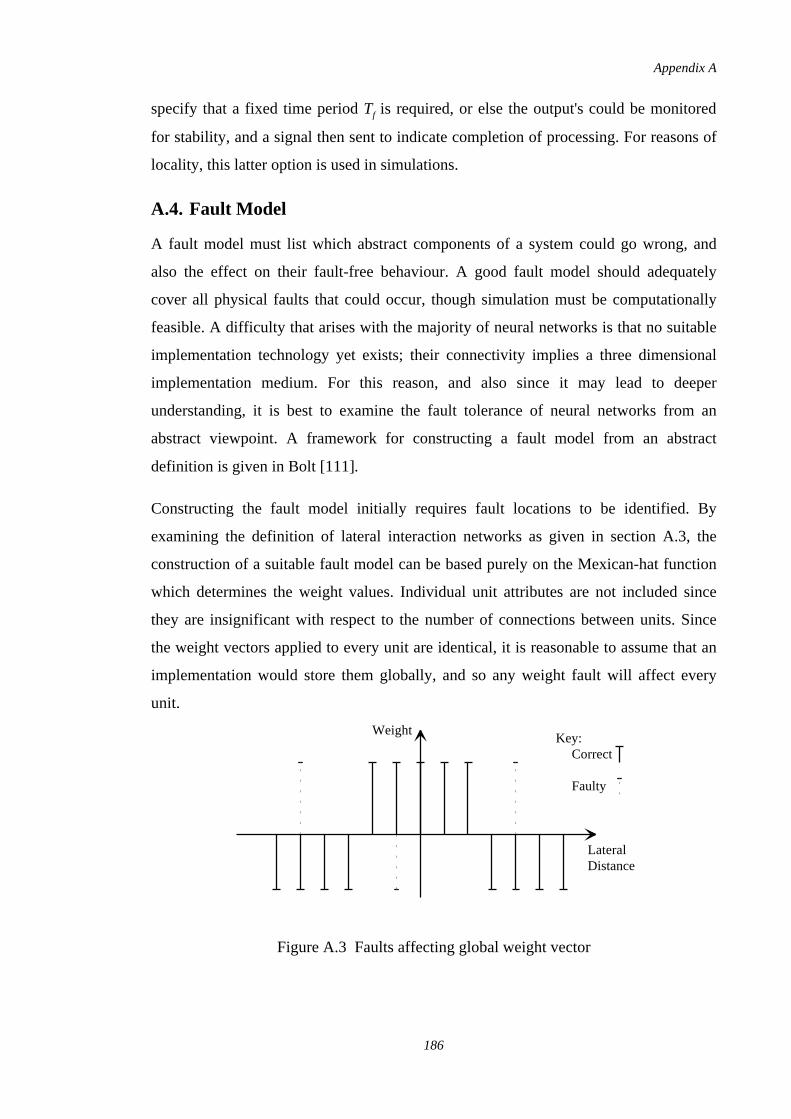
specify that a fixed time period Tf is required, or else the output's could be monitored
for stability, and a signal then sent to indicate completion of processing. For reasons of
locality, this latter option is used in simulations.
A.4. Fault Model
A fault model must list which abstract components of a system could go wrong, and
also the effect on their fault-free behaviour. A good fault model should adequately
cover all physical faults that could occur, though simulation must be computationally
feasible. A difficulty that arises with the majority of neural networks is that no suitable
implementation technology yet exists; their connectivity implies a three dimensional
implementation medium. For this reason, and also since it may lead to deeper
understanding, it is best to examine the fault tolerance of neural networks from an
abstract viewpoint. A framework for constructing a fault model from an abstract
definition is given in Bolt [111].
Constructing the fault model initially requires fault locations to be identified. By
examining the definition of lateral interaction networks as given in section A.3, the
construction of a suitable fault model can be based purely on the Mexican-hat function
which determines the weight values. Individual unit attributes are not included since
they are insignificant with respect to the number of connections between units. Since
the weight vectors applied to every unit are identical, it is reasonable to assume that an
implementation would store them globally, and so any weight fault will affect every
unit.
Figure A.3 Faults affecting global weight vector
WeightKey:
Correct
Faulty
LateralDistance
Appendix A
186
Now that the components of the global weight vector have been identified as the fault
model's locations, it only remains to define faulty behaviour. Operating on the principle
of maximum damage, two failure modes can be constructed for a faulty weight element.
These are stuck-at-0 and inverted. The latter refers to a excitatory connection becoming
inhibitory and vice versa. Note that the loss of a connection is incorporated by default
into the above fault definitions affecting the global weight vector, though more severely
since the matching connection will be lost for every unit. Figure A.3 illustrates faults
affecting a simplified discrete Mexican-hat function.
A.4.1. Timescale
Faults can be classified as either transient or permanent. The lifetime of transient faults
is only some short period of time, but the latter persist forever. By far the most common
are transient faults [104], and it is these that will be modelled in simulations.
The timing of when faults should realistically be introduced, and for how long they
should last must be defined before simulations can be performed. This will depend on
the type of application area as well as the functionality of lateral interaction networks. If
the application involves the use of a lateral interaction network as a component, then its
operation should be viewed as a single step. Any faults should be injected when the
input is initially presented to it, and they should be defined to last for the complete
processing of the input pattern1. However, if a subsequent system is sensitive to changes
in the networks' outputs, or the network is considered as the entire system under
investigation, then any faults should be injected at each iteration of the lateral
interaction process. The duration of faults should last for only one iteration since the
evolution of the output is paramount.
A.5. Definition of Failure
Due to the correspondence between soft applications and the nature of neural networks
computation, failure is not a clearly observable discrete event, rather it is a degradation
in the quality of the solution which is represented by the output's of the neural network.
This implies that a continuous measure of failure is more suitable. Since, as mentioned
in section A.2, even the fault-free response of a neural network may vary around the
1 This case applied to simulations performed.
Appendix A
187
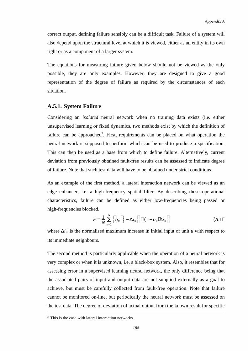
correct output, defining failure sensibly can be a difficult task. Failure of a system will
also depend upon the structural level at which it is viewed, either as an entity in its own
right or as a component of a larger system.
The equations for measuring failure given below should not be viewed as the only
possible, they are only examples. However, they are designed to give a good
representation of the degree of failure as required by the circumstances of each
situation.
A.5.1. System Failure
Considering an isolated neural network when no training data exists (i.e. either
unsupervised learning or fixed dynamics, two methods exist by which the definition of
failure can be approached2. First, requirements can be placed on what operation the
neural network is supposed to perform which can be used to produce a specification.
This can then be used as a base from which to define failure. Alternatively, current
deviation from previously obtained fault-free results can be assessed to indicate degree
of failure. Note that such test data will have to be obtained under strict conditions.
As an example of the first method, a lateral interaction network can be viewed as an
edge enhancer, i.e. a high-frequency spatial filter. By describing these operational
characteristics, failure can be defined as either low-frequencies being passed or
high-frequencies blocked.
where is the normalised maximum increase in initial input of unit u with respect to∆i u
its immediate neighbours.
The second method is particularly applicable when the operation of a neural network is
very complex or when it is unknown, i.e. a black-box system. Also, it resembles that for
assessing error in a supervised learning neural network, the only difference being that
the associated pairs of input and output data are not supplied externally as a goal to
achieve, but must be carefully collected from fault-free operation. Note that failure
cannot be monitored on-line, but periodically the neural network must be assessed on
the test data. The degree of deviation of actual output from the known result for specific
2 This is the case with lateral interaction networks.
F = 1N Σ
u=1
N ou
1 −∆iu
+ (1 − ou)∆i u
(A.1)
Appendix A
188
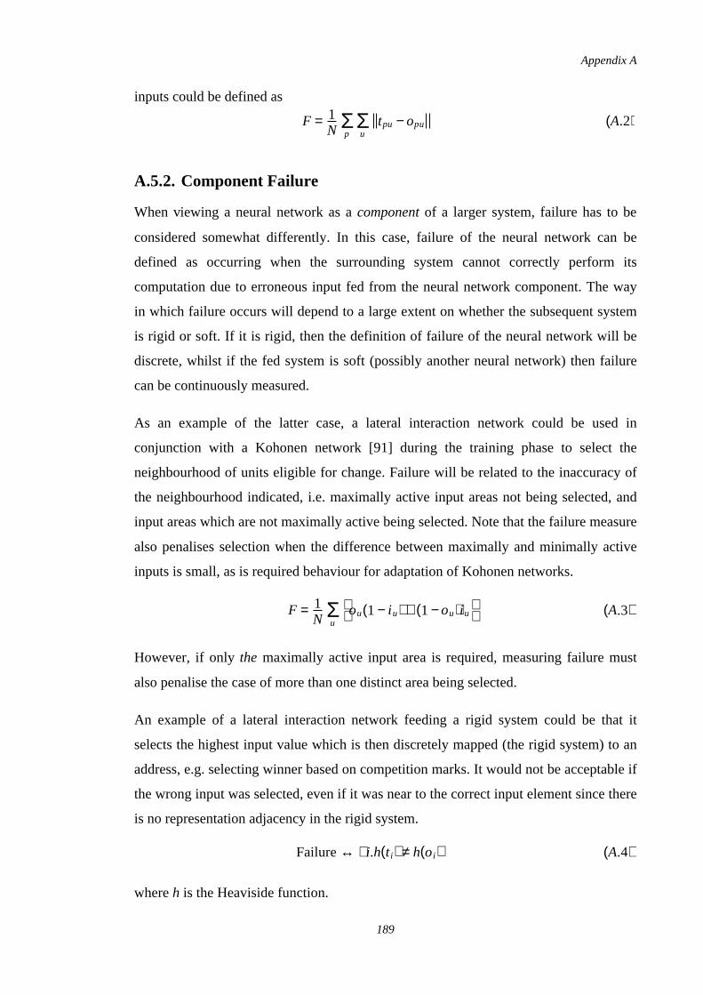
inputs could be defined as
A.5.2. Component Failure
When viewing a neural network as a component of a larger system, failure has to be
considered somewhat differently. In this case, failure of the neural network can be
defined as occurring when the surrounding system cannot correctly perform its
computation due to erroneous input fed from the neural network component. The way
in which failure occurs will depend to a large extent on whether the subsequent system
is rigid or soft. If it is rigid, then the definition of failure of the neural network will be
discrete, whilst if the fed system is soft (possibly another neural network) then failure
can be continuously measured.
As an example of the latter case, a lateral interaction network could be used in
conjunction with a Kohonen network [91] during the training phase to select the
neighbourhood of units eligible for change. Failure will be related to the inaccuracy of
the neighbourhood indicated, i.e. maximally active input areas not being selected, and
input areas which are not maximally active being selected. Note that the failure measure
also penalises selection when the difference between maximally and minimally active
inputs is small, as is required behaviour for adaptation of Kohonen networks.
However, if only the maximally active input area is required, measuring failure must
also penalise the case of more than one distinct area being selected.
An example of a lateral interaction network feeding a rigid system could be that it
selects the highest input value which is then discretely mapped (the rigid system) to an
address, e.g. selecting winner based on competition marks. It would not be acceptable if
the wrong input was selected, even if it was near to the correct input element since there
is no representation adjacency in the rigid system.
where h is the Heaviside function.
F = 1N Σ
pΣu
tpu − opu (A.2)
F = 1N Σ
u
ou(1 − i u) + (1 −ou)i u
(A.3)
Failure ↔ ∃ i.h(t i) ≠ h(oi) (A.4)
Appendix A
189
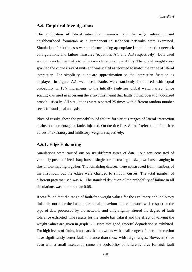
A.6. Empirical Investigations
The application of lateral interaction networks both for edge enhancing and
neighbourhood formation as a component in Kohonen networks were examined.
Simulations for both cases were performed using appropriate lateral interaction network
configurations and failure measures (equations A.1 and A.3 respectively). Data used
was constructed manually to reflect a wide range of variability. The global weight array
spanned the entire array of units and was scaled as required to match the range of lateral
interaction. For simplicity, a square approximation to the interaction function as
displayed in figure A.1 was used. Faults were randomly introduced with equal
probability in 10% increments to the initially fault-free global weight array. Since
scaling was used in accessing the array, this meant that faults during operation occurred
probabilistically. All simulations were repeated 25 times with different random number
seeds for statistical analysis.
Plots of results show the probability of failure for various ranges of lateral interaction
against the percentage of faults injected. On the title line, E and I refer to the fault-free
values of excitatory and inhibitory weights respectively.
A.6.1. Edge Enhancing
Simulations were carried out on six different types of data. Four sets consisted of
variously position/sized sharp bars; a single bar decreasing in size, two bars changing in
size and/or moving together. The remaining datasets were constructed from members of
the first four, but the edges were changed to smooth curves. The total number of
different patterns used was 43. The standard deviation of the probability of failure in all
simulations was no more than 0.08.
It was found that the range of fault-free weight values for the excitatory and inhibitory
links did not alter the basic operational behaviour of the network with respect to the
type of data processed by the network, and only slightly altered the degree of fault
tolerance exhibited. The results for the single bar dataset and the effect of varying the
weight values are given in graph A.1. Note that good graceful degradation is exhibited.
For high levels of faults, it appears that networks with small ranges of lateral interaction
have significantly better fault tolerance than those with large ranges. However, since
even with a small interaction range the probability of failure is large for high fault
Appendix A
190
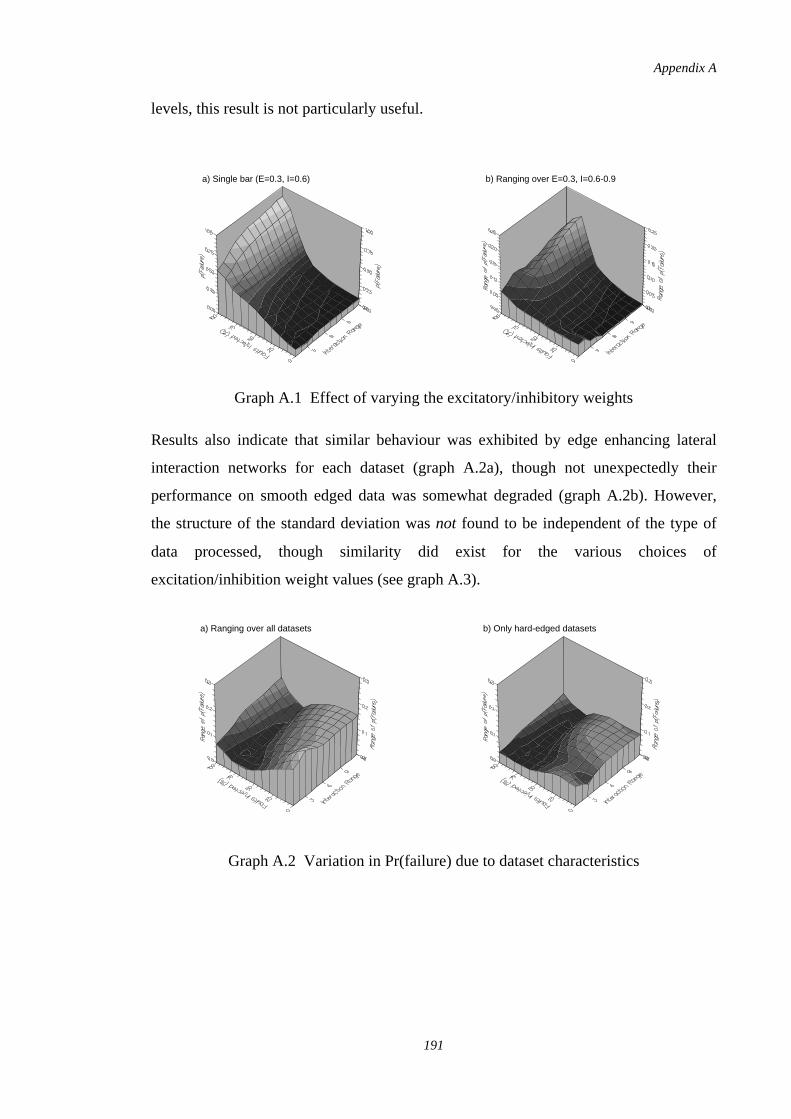
levels, this result is not particularly useful.
Graph A.1 Effect of varying the excitatory/inhibitory weights
Results also indicate that similar behaviour was exhibited by edge enhancing lateral
interaction networks for each dataset (graph A.2a), though not unexpectedly their
performance on smooth edged data was somewhat degraded (graph A.2b). However,
the structure of the standard deviation was not found to be independent of the type of
data processed, though similarity did exist for the various choices of
excitation/inhibition weight values (see graph A.3).
Graph A.2 Variation in Pr(failure) due to dataset characteristics
a) Single bar (E=0.3, I=0.6) b) Ranging over E=0.3, I=0.6-0.9
a) Ranging over all datasets b) Only hard-edged datasets
Appendix A
191
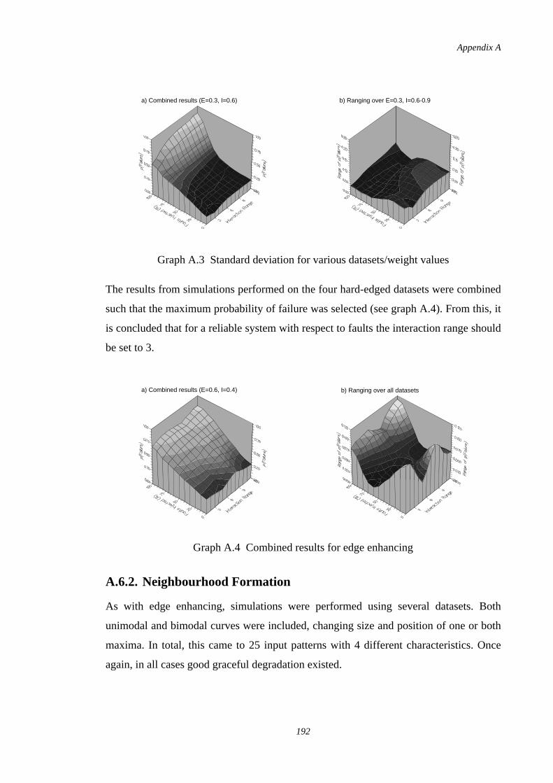
Graph A.3 Standard deviation for various datasets/weight values
The results from simulations performed on the four hard-edged datasets were combined
such that the maximum probability of failure was selected (see graph A.4). From this, it
is concluded that for a reliable system with respect to faults the interaction range should
be set to 3.
Graph A.4 Combined results for edge enhancing
A.6.2. Neighbourhood Formation
As with edge enhancing, simulations were performed using several datasets. Both
unimodal and bimodal curves were included, changing size and position of one or both
maxima. In total, this came to 25 input patterns with 4 different characteristics. Once
again, in all cases good graceful degradation existed.
a) Combined results (E=0.3, I=0.6) b) Ranging over E=0.3, I=0.6-0.9
a) Combined results (E=0.6, I=0.4) b) Ranging over all datasets
Appendix A
192
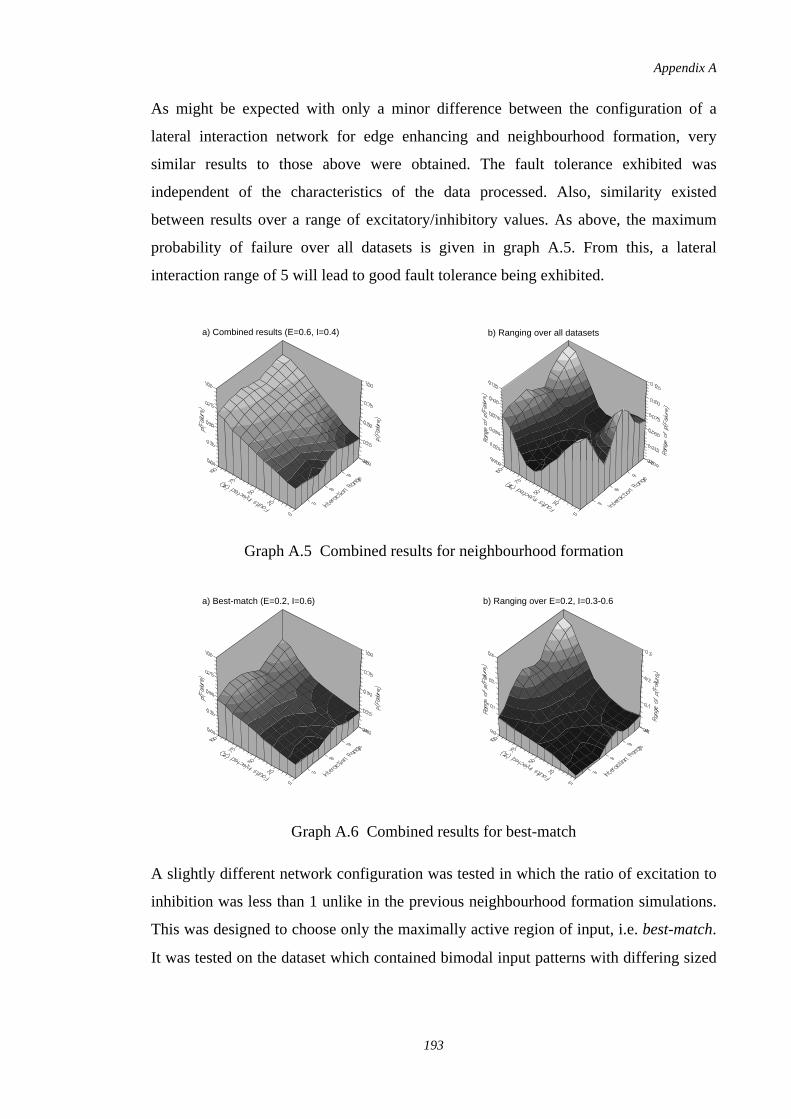
As might be expected with only a minor difference between the configuration of a
lateral interaction network for edge enhancing and neighbourhood formation, very
similar results to those above were obtained. The fault tolerance exhibited was
independent of the characteristics of the data processed. Also, similarity existed
between results over a range of excitatory/inhibitory values. As above, the maximum
probability of failure over all datasets is given in graph A.5. From this, a lateral
interaction range of 5 will lead to good fault tolerance being exhibited.
Graph A.5 Combined results for neighbourhood formation
Graph A.6 Combined results for best-match
A slightly different network configuration was tested in which the ratio of excitation to
inhibition was less than 1 unlike in the previous neighbourhood formation simulations.
This was designed to choose only the maximally active region of input, i.e. best-match.
It was tested on the dataset which contained bimodal input patterns with differing sized
a) Combined results (E=0.6, I=0.4) b) Ranging over all datasets
a) Best-match (E=0.2, I=0.6) b) Ranging over E=0.2, I=0.3-0.6
Appendix A
193

maxima. Results are shown in figure A.6. It is again evident that the functionality is not
influenced greatly by the particular choice of excitation/inhibition weight values.
A.7. Conclusions
The effect of faults on lateral interaction networks functioning both as an edge
enhancing system and a clustering system has been investigated. Results show that the
change in behaviour due to faults is not influenced by the type of data processed.
Similarly the operational quality is not altered drastically over a range of values for the
excitation and inhibition weights. Selection of the interaction range appears to be the
most critical element in designing a fault tolerant system, though here again results have
shown that some flexibility exists.
The similarity of behaviour over a wide range of parameters and data presented
suggests that lateral interaction networks provide a robust system against faults and also
external noise. Also, graceful degradation is exhibited as the level of faults increases.
Appendix A
194
APPENDIX B
Glossary
This appendix presents an extended glossary of terms used in this thesis.
Activation This is the internal state of an unit in a neural network formed
from its combined weighted inputs before thresholding is
applied.
Classification Inputs are labelled as belonging to one of a discrete number
of types or classes. A null class is sometimes included to
represent unknown inputs.
Computation Fault
Tolerance
Resistance to effect of faults to computation performed by
abstracted system.
Data Representation The format of external inputs presented to a neural network.
Distribution Refers to holistic nature of a neural network's operation and
information storage. All components of a neural network are
involved during training and operation. No part of a neural
network's function can be attributed to a local region in its
architecture.
Appendix B
195

Epoch Completion of a training pass. Often applied to supervised
training to refer to presentation of entire training set.
Error An internal result in a system's computation which is likely to
lead to failure.
Failure Event that the operation of a system no longer meets its
required specification.
Failure Rate Constant applied to components describing the rate at which
they become defective. Defined as the number of components
failing from time t0 to t1 relative to the original number of
surviving components at time to.
Faults The cause of an error. For example, defects occurring in a
systems' components, erroneous inputs, design inaccuracies.
Fault Model Abstractly describes the effect of physical defects on a
system's operation.
Fault Tolerance A technique used to increase the reliability of a system by
imbuing it with resilience to the effect of faults occurring.
Feedback Neural
Network
A neural network which has loops in its connectivity, i.e.
internal feedback exists.
Feedforward Neural
Network
A neural network which has no loops in its connectivity, i.e.
no internal feedback exists.
Appendix B
196
Function
Approximation
Type of problem given to neural network. Requires it to learn
a continuous or discrete mapping between two vector spaces.
Generalisation Refers to the ability of a neural network to produce a sensible
output for an input which did not occur during training.
Graceful DegradationProperty of a system to deliver useful service in the presence
of faults.
Hidden Units Processing units in a neural network both only fed by and
feeding other processing units within the neural network.
Internal
Representation
The representation of a problem formed in the hidden units of
a neural network during learning. Points in the hidden unit
space are mapped from points in the input space.
Learning Algorithm Constructive method by which the free parameters in a neural
network can be changed so that it solves a given problem.
Modular Neural
Networks
Systems composing of several smaller neural networks which
are individually trained and operated.
N-Modular
Redundancy
A fault tolerance mechanism which duplicates of a sub-
system N times, and then takes a majority vote to determine
the final output.
Neural Network A large number of simple processing elements with complex
interconnectivity. Has basis in biological neural systems.
Appendix B
197
Recurrent Neural
Network
See Feedback Neural Network.
Redundancy Spare capacity in a system either to actively or passively
broaden computational load. When applied to data it allows
reconstruction of damaged entries. In duplicating sub-system
processing, overall system operation no longer requires the
correct operation of all system components. Often introduced
to a system by fault tolerance techniques.
Reliability Probability of a system operating correctly at time t.
Rigid .vs. Soft
Problem
Classification of problems based on the degree of adjacency
existing in their solution space. Soft problems are described
by a large adjacency factor, rigid problems are not.
Squashing Function See Thresholding Function.
Thresholding
Function
Function applied to a units activation to form its output.
Limits absolute magnitude of a unit's activation.
Training Cycle See Epoch.
Training Set Set of input, output pairs used during the supervised training
of a neural network.
Appendix B
198
Tuple Unit A function taking a n dimensional binary input i coding an
integer a in the range [0,2n], and producing a 2n dimensional
binary input with a 1 in the position corresponding to a, and
0's in the remainder. For example, 010 maps to 00000100.
Uniform Information
Distribution
As for distribution of information, but computational load of
neural networks' elements equal.
Weight Scalar value associated with a connection between two units
which modifies the communicated data. Generally acts as a
multiplicative factor.
Appendix B
199
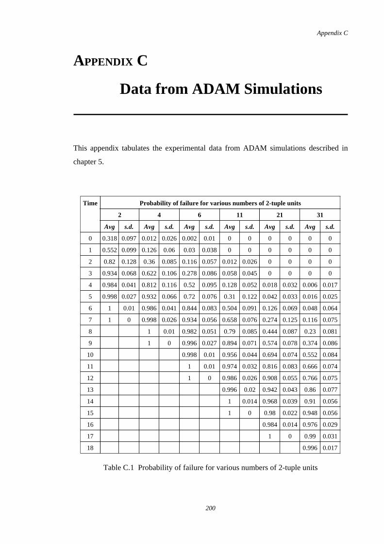
APPENDIX C
Data from ADAM Simulations
This appendix tabulates the experimental data from ADAM simulations described in
chapter 5.
Time Probability of failure for various numbers of 2-tuple units
2 4 6 11 21 31
Avg s.d. Avg s.d. Avg s.d. Avg s.d. Avg s.d. Avg s.d.
0 0.318 0.097 0.012 0.026 0.0020.01 0 0 0 0 0 0
1 0.552 0.099 0.126 0.06 0.03 0.038 0 0 0 0 0 0
2 0.82 0.128 0.36 0.085 0.116 0.057 0.012 0.026 0 0 0 0
3 0.934 0.068 0.622 0.106 0.278 0.086 0.058 0.0450 0 0 0
4 0.984 0.041 0.812 0.1160.52 0.095 0.128 0.052 0.018 0.032 0.006 0.017
5 0.998 0.027 0.932 0.0660.72 0.076 0.31 0.122 0.042 0.033 0.016 0.025
6 1 0.01 0.986 0.041 0.844 0.083 0.504 0.091 0.126 0.069 0.048 0.064
7 1 0 0.998 0.026 0.934 0.056 0.658 0.076 0.274 0.125 0.116 0.075
8 1 0.01 0.982 0.051 0.79 0.085 0.444 0.087 0.23 0.081
9 1 0 0.996 0.027 0.894 0.071 0.574 0.078 0.374 0.086
10 0.998 0.01 0.956 0.044 0.694 0.074 0.552 0.084
11 1 0.01 0.974 0.032 0.816 0.083 0.666 0.074
12 1 0 0.986 0.026 0.908 0.055 0.766 0.075
13 0.996 0.02 0.942 0.043 0.86 0.077
14 1 0.014 0.968 0.039 0.91 0.056
15 1 0 0.98 0.022 0.948 0.056
16 0.984 0.014 0.976 0.029
17 1 0 0.99 0.031
18 0.996 0.017
Table C.1 Probability of failure for various numbers of 2-tuple units
Appendix C
200
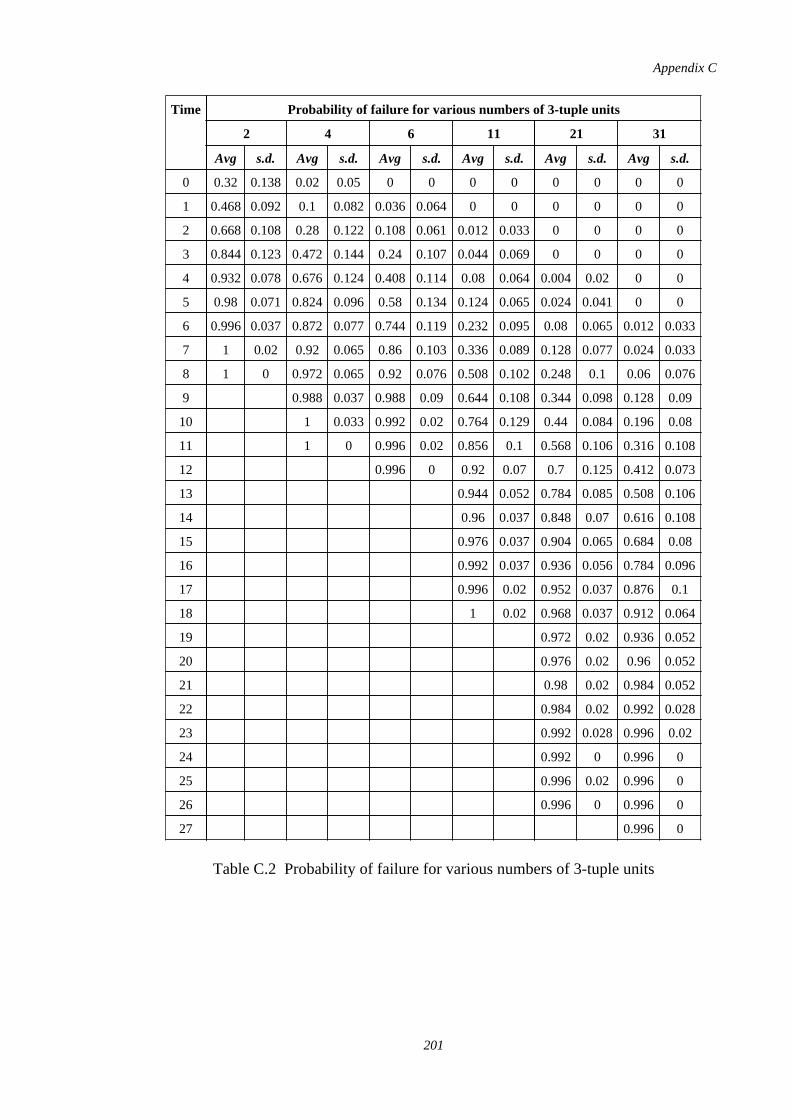
Time Probability of failure for various numbers of 3-tuple units
2 4 6 11 21 31
Avg s.d. Avg s.d. Avg s.d. Avg s.d. Avg s.d. Avg s.d.
0 0.32 0.138 0.02 0.05 0 0 0 0 0 0 0 0
1 0.468 0.092 0.1 0.082 0.036 0.064 0 0 0 0 0 0
2 0.668 0.108 0.28 0.122 0.108 0.061 0.012 0.033 0 0 0 0
3 0.844 0.123 0.472 0.1440.24 0.107 0.044 0.069 0 0 0 0
4 0.932 0.078 0.676 0.124 0.408 0.1140.08 0.064 0.004 0.02 0 0
5 0.98 0.071 0.824 0.096 0.58 0.134 0.124 0.065 0.024 0.041 0 0
6 0.996 0.037 0.872 0.077 0.744 0.119 0.232 0.0950.08 0.065 0.012 0.033
7 1 0.02 0.92 0.065 0.86 0.103 0.336 0.089 0.128 0.077 0.024 0.033
8 1 0 0.972 0.065 0.92 0.076 0.508 0.102 0.248 0.1 0.06 0.076
9 0.988 0.037 0.988 0.09 0.644 0.108 0.344 0.098 0.1280.09
10 1 0.033 0.992 0.02 0.764 0.129 0.44 0.084 0.196 0.08
11 1 0 0.996 0.02 0.856 0.1 0.568 0.106 0.316 0.108
12 0.996 0 0.92 0.07 0.7 0.125 0.412 0.073
13 0.944 0.052 0.784 0.085 0.508 0.106
14 0.96 0.037 0.848 0.07 0.616 0.108
15 0.976 0.037 0.904 0.065 0.6840.08
16 0.992 0.037 0.936 0.056 0.784 0.096
17 0.996 0.02 0.952 0.037 0.876 0.1
18 1 0.02 0.968 0.037 0.912 0.064
19 0.972 0.02 0.936 0.052
20 0.976 0.02 0.96 0.052
21 0.98 0.02 0.984 0.052
22 0.984 0.02 0.992 0.028
23 0.992 0.028 0.996 0.02
24 0.992 0 0.996 0
25 0.996 0.02 0.996 0
26 0.996 0 0.996 0
27 0.996 0
Table C.2 Probability of failure for various numbers of 3-tuple units
Appendix C
201
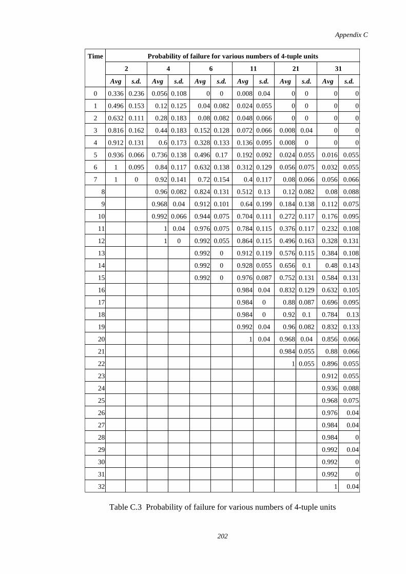
Time Probability of failure for various numbers of 4-tuple units
2 4 6 11 21 31
Avg s.d. Avg s.d. Avg s.d. Avg s.d. Avg s.d. Avg s.d.
0 0.336 0.236 0.056 0.108 0 0 0.008 0.04 0 0 0 0
1 0.496 0.153 0.12 0.125 0.04 0.082 0.024 0.055 0 0 0 0
2 0.632 0.111 0.28 0.183 0.08 0.082 0.048 0.066 0 0 0 0
3 0.816 0.162 0.44 0.183 0.152 0.128 0.072 0.066 0.0080.04 0 0
4 0.912 0.131 0.6 0.173 0.328 0.133 0.136 0.095 0.0080 0 0
5 0.936 0.066 0.736 0.138 0.4960.17 0.192 0.092 0.024 0.055 0.016 0.055
6 1 0.095 0.84 0.117 0.632 0.138 0.312 0.129 0.056 0.075 0.032 0.055
7 1 0 0.92 0.141 0.72 0.154 0.4 0.117 0.08 0.066 0.056 0.066
8 0.96 0.082 0.824 0.131 0.5120.13 0.12 0.082 0.08 0.088
9 0.968 0.04 0.912 0.101 0.64 0.199 0.184 0.138 0.112 0.075
10 0.992 0.066 0.944 0.075 0.704 0.111 0.272 0.117 0.176 0.095
11 1 0.04 0.976 0.075 0.784 0.115 0.376 0.117 0.232 0.108
12 1 0 0.992 0.055 0.864 0.115 0.496 0.163 0.328 0.131
13 0.992 0 0.912 0.119 0.576 0.115 0.384 0.108
14 0.992 0 0.928 0.055 0.656 0.1 0.48 0.143
15 0.992 0 0.976 0.087 0.752 0.131 0.584 0.131
16 0.984 0.04 0.832 0.129 0.632 0.105
17 0.984 0 0.88 0.087 0.696 0.095
18 0.984 0 0.92 0.1 0.784 0.13
19 0.992 0.04 0.96 0.082 0.832 0.133
20 1 0.04 0.968 0.04 0.856 0.066
21 0.984 0.055 0.88 0.066
22 1 0.055 0.896 0.055
23 0.912 0.055
24 0.936 0.088
25 0.968 0.075
26 0.976 0.04
27 0.984 0.04
28 0.984 0
29 0.992 0.04
30 0.992 0
31 0.992 0
32 1 0.04
Table C.3 Probability of failure for various numbers of 4-tuple units
Appendix C
202
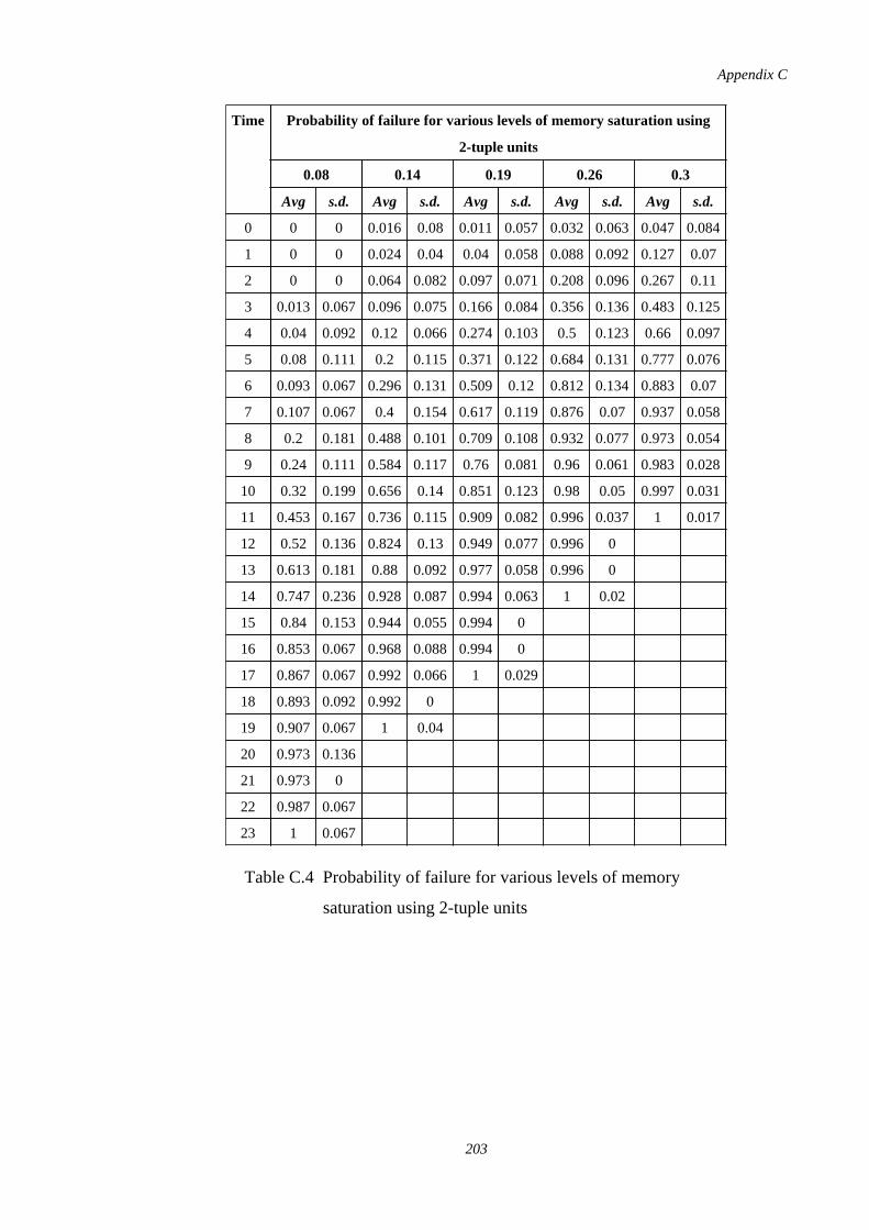
Time Probability of failure for various levels of memory saturation using
2-tuple units
0.08 0.14 0.19 0.26 0.3
Avg s.d. Avg s.d. Avg s.d. Avg s.d. Avg s.d.
0 0 0 0.016 0.08 0.011 0.057 0.032 0.063 0.047 0.084
1 0 0 0.024 0.04 0.04 0.058 0.088 0.092 0.1270.07
2 0 0 0.064 0.082 0.097 0.071 0.208 0.096 0.2670.11
3 0.013 0.067 0.096 0.075 0.166 0.084 0.356 0.136 0.483 0.125
4 0.04 0.092 0.12 0.066 0.274 0.103 0.5 0.123 0.66 0.097
5 0.08 0.111 0.2 0.115 0.371 0.122 0.684 0.131 0.777 0.076
6 0.093 0.067 0.296 0.131 0.5090.12 0.812 0.134 0.883 0.07
7 0.107 0.067 0.4 0.154 0.617 0.119 0.8760.07 0.937 0.058
8 0.2 0.181 0.488 0.101 0.709 0.108 0.932 0.077 0.973 0.054
9 0.24 0.111 0.584 0.117 0.76 0.081 0.96 0.061 0.983 0.028
10 0.32 0.199 0.656 0.14 0.851 0.123 0.98 0.05 0.997 0.031
11 0.453 0.167 0.736 0.115 0.909 0.082 0.996 0.0371 0.017
12 0.52 0.136 0.824 0.13 0.949 0.077 0.996 0
13 0.613 0.181 0.88 0.092 0.977 0.058 0.996 0
14 0.747 0.236 0.928 0.087 0.994 0.063 1 0.02
15 0.84 0.153 0.944 0.055 0.994 0
16 0.853 0.067 0.968 0.088 0.994 0
17 0.867 0.067 0.992 0.066 1 0.029
18 0.893 0.092 0.992 0
19 0.907 0.067 1 0.04
20 0.973 0.136
21 0.973 0
22 0.987 0.067
23 1 0.067
Table C.4 Probability of failure for various levels of memory
saturation using 2-tuple units
Appendix C
203
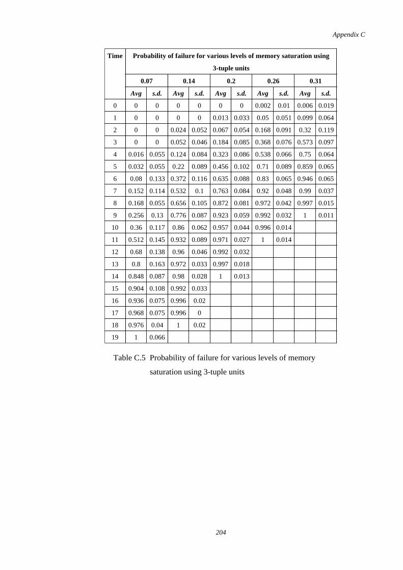
Time Probability of failure for various levels of memory saturation using
3-tuple units
0.07 0.14 0.2 0.26 0.31
Avg s.d. Avg s.d. Avg s.d. Avg s.d. Avg s.d.
0 0 0 0 0 0 0 0.002 0.01 0.006 0.019
1 0 0 0 0 0.013 0.033 0.05 0.051 0.099 0.064
2 0 0 0.024 0.052 0.067 0.054 0.168 0.0910.32 0.119
3 0 0 0.052 0.046 0.184 0.085 0.368 0.076 0.573 0.097
4 0.016 0.055 0.124 0.084 0.323 0.086 0.538 0.0660.75 0.064
5 0.032 0.055 0.22 0.089 0.456 0.102 0.71 0.089 0.859 0.065
6 0.08 0.133 0.372 0.116 0.635 0.0880.83 0.065 0.946 0.065
7 0.152 0.114 0.532 0.1 0.763 0.084 0.92 0.048 0.99 0.037
8 0.168 0.055 0.656 0.105 0.872 0.081 0.972 0.042 0.997 0.015
9 0.256 0.13 0.776 0.087 0.923 0.059 0.992 0.032 1 0.011
10 0.36 0.117 0.86 0.062 0.957 0.044 0.996 0.014
11 0.512 0.145 0.932 0.089 0.971 0.027 1 0.014
12 0.68 0.138 0.96 0.046 0.992 0.032
13 0.8 0.163 0.972 0.033 0.997 0.018
14 0.848 0.087 0.98 0.028 1 0.013
15 0.904 0.108 0.992 0.033
16 0.936 0.075 0.996 0.02
17 0.968 0.075 0.996 0
18 0.976 0.04 1 0.02
19 1 0.066
Table C.5 Probability of failure for various levels of memory
saturation using 3-tuple units
Appendix C
204
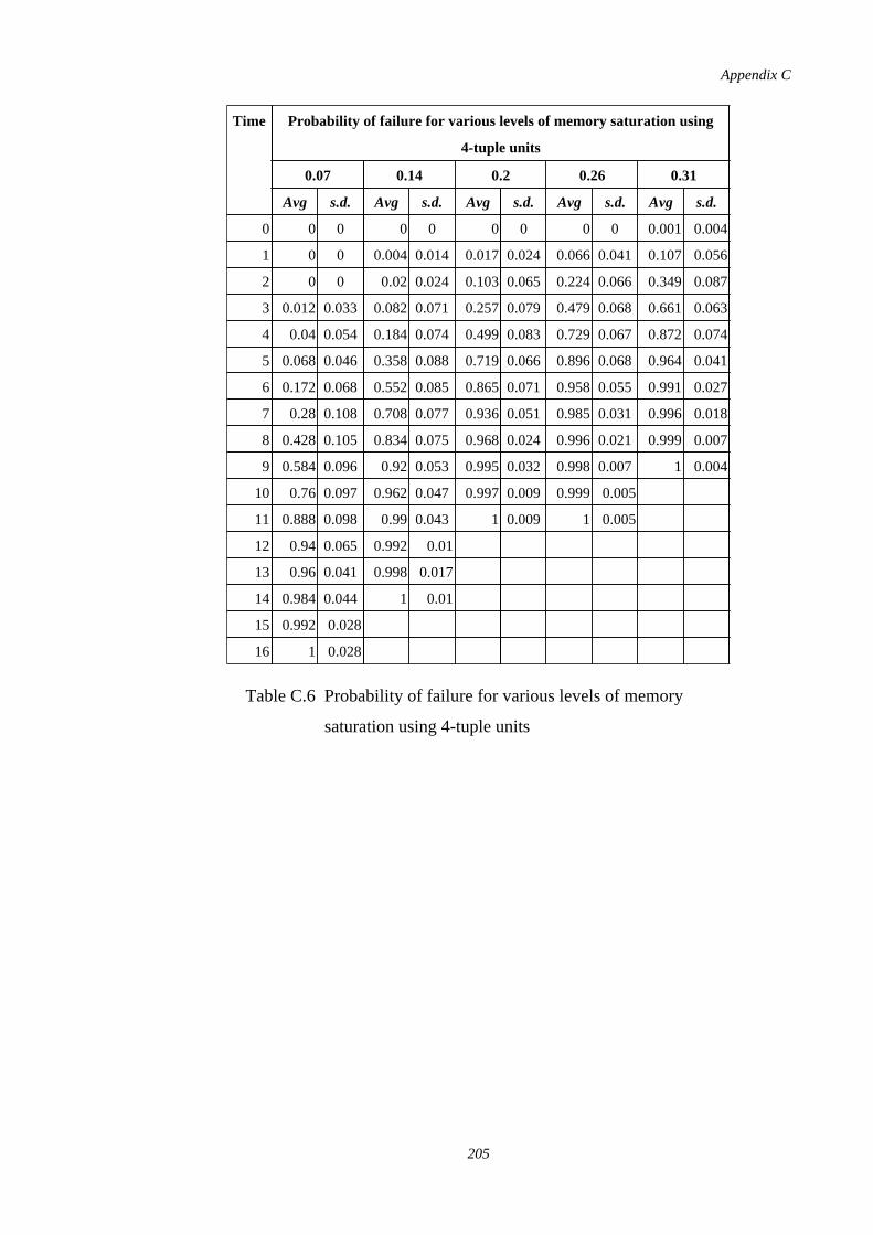
Time Probability of failure for various levels of memory saturation using
4-tuple units
0.07 0.14 0.2 0.26 0.31
Avg s.d. Avg s.d. Avg s.d. Avg s.d. Avg s.d.
0 0 0 0 0 0 0 0 0 0.001 0.004
1 0 0 0.004 0.014 0.017 0.024 0.066 0.041 0.107 0.056
2 0 0 0.02 0.024 0.103 0.065 0.224 0.066 0.349 0.087
3 0.012 0.033 0.082 0.071 0.257 0.079 0.479 0.068 0.661 0.063
4 0.04 0.054 0.184 0.074 0.499 0.083 0.729 0.067 0.872 0.074
5 0.068 0.046 0.358 0.088 0.719 0.066 0.896 0.068 0.964 0.041
6 0.172 0.068 0.552 0.085 0.865 0.071 0.958 0.055 0.991 0.027
7 0.28 0.108 0.708 0.077 0.936 0.051 0.985 0.031 0.996 0.018
8 0.428 0.105 0.834 0.075 0.968 0.024 0.996 0.021 0.999 0.007
9 0.584 0.096 0.92 0.053 0.995 0.032 0.998 0.007 1 0.004
10 0.76 0.097 0.962 0.047 0.997 0.009 0.999 0.005
11 0.888 0.098 0.99 0.043 1 0.009 1 0.005
12 0.94 0.065 0.992 0.01
13 0.96 0.041 0.998 0.017
14 0.984 0.044 1 0.01
15 0.992 0.028
16 1 0.028
Table C.6 Probability of failure for various levels of memory
saturation using 4-tuple units
Appendix C
205
REFERENCES
1. Beale, R. and Jackson, T., Neural Computing: An Introduction, IOP Publishing
(1990).
2. Lippmann, R.P., "An introduction to computing with neural nets", IEEE
Acoustics Speech Signal Processing Magazine 4, pp.4-22 (1987).
3. Khanna, T., Foundation of Neural Networks, Addison-Wesley (1990).
4. Lala, P.K., Fault Tolerant and Fault Testable Hardware Design, (1985).
5. Kaufmann, A., Reliability - A Mathematical Approach, Transworld Publishers,
London (1972).
6. Anderson, T. and Lee, P.A., Fault Tolerance, principles and practice,
Prentice-Hall International (1981).
7. Amit, D.J. and Gutfreund, H., "Statistical Mechanics of Neural Networks near
Saturation", Annals of Physics 173, pp.30-67 (1987).
8. Anderson, J.A., "Cognitive and Psychological Computation with Neural Models",
IEEE Trans Systems Man and Cybernetics SMC-13, pp.799-815 (1983).
9. Baum, E.B., Moody, J. and Wilczek, F., "Internal Representations for Associative
Memory", Biological Cybernetics 59, pp.217-228 (1988).
10. Bruce, A., Canning, A., Forrest, B., Gardner, E., Wallace, D.J., 1986, 65-70 and
AIP Conference Proceedings 151, "Learning and Memory Properties in Fully
Connected Networks", AIP Conference Proceedings 151, pp.65-70 (1986).
11. Fogelman-Soulie, F., Gallinari, P., Le Cun, Y. and Thiria, S., "Evaluation of
network architectures on test learning tasks", Proceedings of the first IEEE
International Conference on Neural Networks, San-Diego II , pp.653-660 (1987).
12. Cannon, S.C., Robinson, D.A. and Shamma, S., "A Proposed Neural Network for
the Integrator of the Oculomotor System", Biological Cybernetics 49, pp.127-36
(1983).
References
206
13. Hopfield, J.J., "Neural networks and physical systems with emergent collective
computational abilities", Proceedings of the National Acadamy of Sciences, USA
79, pp.2554-8 (1982).
14. Kung, S.Y., "Parallel Architectures for Artificial Neural Nets", Proc.
International Conference on Systolic Arrays, pp.163-74 (1988).
15. Legendy, C.R., "On the Scheme by Which the Human Brain Stores Information",
Mathematical Biosciences 1, pp.555-97 (1967).
16. Char, J.M., Cherkassy, V., Wechsler, H. and Zimmerman, G.L., "Distributed and
fault-tolerant computation for retrieval tasks using distributed associative
memories", IEEE Transactions on Computers A15(4), pp.484-90 (April 1988).
17. Worden, S.J. and Womack, B.F., "Analysis of small compacta networks",
Proceedings of 1986 IEEE Conference on Systems, Man and Cybernetics, pp.61-4
(1986).
18. Zhou, Y.T., Chellappa, R. and Jenkins, B.K., "A Novel Approach to Image
Restoration Based on a Neural Network", Proceeding of the IEEE First Annual
International Conference on Neural Networks 4, pp. 269-76 (1987).
19. Carter, M.J., "The 'Illusion' of Fault Tolerance in Neural Networks for Pattern
Recognition and Signal Processing", Proc. Technical Session on Fault-Tolerant
Integrated Systems, Durham NH: University of New Hampshire (1988).
20. Bedworth, M.D. and Lowe, D., Fault Tolerance in Multi-Layer Perceptrons: a
preliminary study, RSRE: Pattern Processing and Machine Intelligence Division
(July 1988).
21. Rumelhart, D.E., Hinton, G.E. and Williams, R.J., "Learning Internal
Representations by Error Propagation" pp. 318-362 in Parallel Distributed
Processing, ed. Rumelhart, D.E. and McClelland, J.L. (Eds), MIT Press (1986).
22. Belfore, L.A. and Johnson, B.W., "The fault-tolerance of neural networks", The
International Journal of Neural Networks Research and Applications 1, pp.24-41
(Jan 1989).
23. Warkowski, F., Leenstra, J., Nijhuis, J. and Spaanenburg, L., "Issues in the Test
of Artificial Neural Networks", Digest ICCD '89, pp.487-490 (Oct 1989).
24. Hinton, G.E. and Shallice, T., "Lesioning an Attractor Network: Investigations of
Acquired Dyslexia", Psychological Review 98(1), pp.74-94 (1991).
References
207
25. Carter, M.J., Rudolph, F. and Nucci, A., "Operational Fault Tolerance of CMAC
Networks", NIPS-90, Denver, Morgan Kaufmann (1990).
26. Segee, B.E. and Carter, M.J., "Comparitive Fault Tolerance of Parallel
Distributed Processing Networks (Debunking the Myth of Inherent Fault
Tolerance)", Intelligent Structures Group Report ECE.IS.92.07 (1992).
27. Protzel, P.W., Palumbo, D.L. and Arras, M.K., "Performance and
Fault-Tolerance of Neural Networks for Optimization", ICASE Report No. 91-45,
NASA Langley Research Centre (1991).
28. Neti, C., Schneider, M.H. and Young, E.D., "Maximally fault-tolerant neural
networks and nonlinear programming", Proceedings of IJCNN-90, San Diego 2,
pp.483-496 (June 1990).
29. Bugmann, G., Sojka, P., Reiss, M., Plumbley, M. and Taylor, J.G., "Direct
Approaches to Improving the Robustness of Multilayer Neural Networks",
Proceedings of the International Conference on Artificial Neural Networks,
Brighton UK (1992).
30. Lansner, A. and Ekeburg, O., "Reliability and Speed of Recall in an Associative
Network", IEEE Trans Pattern Analysis and Machine Intelligence PAMI-7(1985).
31. Nijhuis, J.A.G. and Spaanenburg, L., "Fault tolerance of neural associative
memories", IEE Proceedings 136-E(5), pp.389-394 (Sept 1989).
32. Heng-Ming, T., "Fault Tolerance in Neural Networks", WNN-AIND-90, pp.59
(Feb 1990).
33. Damarla, T.R. and Bhagat, P.K., "Fault Tolerance in Neural Networks",
Southeastcon '89 Proceedings: Energy and Information Technologies in the S.E.
1, pp.328-31 (1989).
34. Prater, J.S. and Morley Jr., R.E., "Characterization of Fault Tolerance in
Feedforward Neural Networks", submitted to IEEE Transactions on Neural
Networks, in review.
35. May, N. and Hammerstrom, D., "Fault Simulation of a Wafer-Scale Integrated
Neural Network", Abstracts of the First INNS Meeting, Boston, pp.393 (1988).
36. Moore, W.R., "Conventional Fault-Tolerance and Neural Computers" pp. 29-37
in Neural Computers, ed. C von der Malsburg, Berlin: Springer-Verlag (1988).
References
208
37. von Seelen, W. and Mallot, H.A., "Parallelism and Redundancy in Neural
Networks" pp. 50-60 in Neural Computers, ed. C von der Malsburg, Berlin:
Springer-Verlag (1988).
38. McCulloch, W.S., "The Reliability of Biological Systems", Self-Organzing
Systems, pp.264-281 (1959).
39. von Neumann, J., "Probabilistic Logics and the Synthesis of Reliable Components
from Unreliable Elements" pp.43-98 in Automata Studies, ed. Shannon, C.E. and
McCarthy, J., Princeton University Press (1956).
40. Izui, Y. and Pentland, A., "Analysis of Neural Networks with Redundancy",
Neural Computation 2(2), pp.226-238 (Summer 1990).
41. Clay, R.D. and Sequin, C.H., "Limiting Fault-Induced Output Errors in ANN's",
IJCNN-91, Seattle, supplementary poster session (1991).
42. Lincoln, W. and Skrzypek, J., "Synergy of Clustering Multiple Back Propagation
Networks", Proceedings of NIPS-89, pp.650-657 (1989).
43. Chu, L. and Wah, B.W., "Fault Tolerant Neural Networks with Hybrid
Redundancy", IJCNN-90, San Diego 2, pp.639-649 (1990).
44. Distante, F., Sami, M.G., Stefanelli, R. and Gajani, G.S., "Fault-Tolerance
Aspects in Silicon Structures for Neural Networks", NIMES-90, pp.284-295
(1990).
45. Fernandes, P.M.L. and Silva, K.M.C., "Nerve cell soma model with high
reliability and low power consumption", Med. & Biol. Eng. & Comput. 18,
pp.261-264 (1980).
46. Biswas, S. and Venkatesh, S.S., "The Devil and the Network: What Sparsity
Implies to Robustness and Memory", NIPS-3, pp.883-889 (1991).
47. Austin, J., "ADAM:A Distributed Associative Memory For Scene Analysis" pp.
285 in Proceedings of first international conference on neural networks, ed.
M.Caudill, C.Butler, IEEE, San Diego (June, 1987).
48. Anderson, J., "Neural models with cognitive implications." pp. 27-90 in Basic
processes in reading perception and comprehension, ed. D. LaBerge and S. J.
Sanuels , Erlbaum (1977).
49. Wood, C., "Implications of simulated lesion experiments for the interpretation of
lesions in real nervous systems" in Neural Models of Language Processes, ed.
Arbib, M.A., Caplan, D. and Marshall, J.C., New York: Academic (1983).
References
209
50. Venkatesh, S.S., "Epsilon Capacity of Neural Networks", AIP Conference
Proceedings 151, pp.440-445 (1986).
51. Tanaka, H., Matsuda, S. and Ogi, H., "Redundant Coding for Fault Tolerant
Computing on Hopfield Network", Abstracts of the First Annual INNS Meeting,
Boston, pp.141 (1988).
52. Miikkulainen, R. and Dyer, M., "Encoding Input/Output Representations in
Connectionist Cognitive Systems", 1988 Connectionist Models Summer School,
Carnegie-Mellon University, Morgan Kaufmann (1988).
53. Takeda, M. and Goodman, J.W., "Neural Networks for computation: number
representations and programming complexity", Applied Optics 25 (1986).
54. Hancock, P., "Data representation in neural nets: an empirical study", 1988
Connectionist Models Summer School, Carnegie-Mellon University, Morgan
Kaufmann (1988).
55. Abu-Mostafa, Y.S., "Neural Networks for Computing?", AIP Conference
Proceedings 151, pp.1-7 (1986).
56. Abu-Mostafa, Y.S., "Complexity of random problems" in Complexity in
Information Theory, Springer-Verlag (1986).
57. Hartley, R. and Szu, H., "A Comparison of the Computational Power of Neural
Network Models", Proceedings of the first IEEE International Conference on
Neural Networks, San-Diego 3, pp.15-22 (1987).
58. Baum, E.B. and Haussler, D., "What Size Net gives Valid Generalization?",
NIPS-89, Denver, Morgan Kaufmann (1987).
59. Vapnik, V.N. and Chervonenkis, A., "On the uniform convergence of relative
frequencies of events to their probabilities", Theory Prob. Appl. 16, pp.264-280
(1971).
60. Segee, B.E. and Carter, M.J., "Fault Tolerance of Pruned Multilayer Networks",
IJCNN-91, Seattle 2, pp.447-452 (1991).
61. Krauth, W., Mezard, M. and Nadal, J.P., "Basins of Attraction in a
Perceptron-Like Neural Network", Complex Systems 2, pp.387-408 (1988).
62. McCulloch, W.S. and Pitts, A., "A logical calculus of the ideas immanent in
nervous activity", Bulletin of Mathematical Biophysics 5, pp.115-133 (1943).
63. Rosenblatt, F., Principles of Neurodynamics, (1962).
References
210
64. Minsky, M. and Papert, S., Perceptrons: An introduction to computational
geometry, MIT Press (1969).
65. Holt, J.L. and Hwang, J., "Finite Precision Error Analysis of Neural Network
Hardware Implementations", FT-10, Dept. of Elect. Engr., University of
Washington (1990).
66. Pemberton, J.C. and Vidal, J.J., "The effect of training signal errors on node
learning", Technical Report: CSD-890041, University of California (1989).
67. Hodges, R.E. and Wu, C., "The Neural Network Self-Healing Process by using a
Reconstructed Sample Space", WNN-AIND-90, pp.65 (1990).
68. Petsche, T. and Dickinson, B.W., "Trellis Codes, Receptive Fields, and Fault
Tolerant, Self-Repairing Neural Networks", IEEE Transactions on Neural
Networks 1 (2), pp.154-166 (1990).
69. Pons, T.P., Garraghty, P.E., Ommaya, A.K., Kaas, J.H., Taub, E. and Mishkin,
M., "Massive Cortical Reorganization After Sensory Deafferentation in Adult
Macaques", Science 252, pp.1857-1860 (1991).
70. Tanaka, H., "A Study of a High Reliable System against Electric Noises and
Element Failures", Proceedings of the 1989 International Symposium on Noise
and Clutter Rejection in Radars and Imaging Sensors, pp.415-20 (1989).
71. Sequin, C. and Clay, D., "Fault-Tolerance in Artificial Neural Networks", Proc.
IJCNN 90, San Diego 1, pp.703-708 (June 1990).
72. Plaut, D.C., "Connectionist Neuropsychology: The Breakdown and Recovery of
Behaviour in Lesioned Attractor Networks", Thesis Summary, (1991).
73. Brause, R., "Fault Tolerance in Neural Network Associative Memory", Technical
Report, Johann Wolfgang Goethe University (1989).
74. Palumbo, D., "Assessing the Fault Tolerance of Neural Networks",
WNN-AIND-90, pp.3 (Feb 1990).
75. Sivilotti, M.A., Emerling, M.R. and Mead, C.A., "VLSI Architectures for
Implementation of Neural Networks", AIP Conference Proceedings 151,
pp.408-413 (1986).
76. McEliece, R.J., Posner, E., Rodemich, E. and Venkatesh, S., "The Capacity of the
Hopfield Associative Memory", IEEE Trans. Info. Theory IT-33, pp.461-82
(1987).
References
211
77. Protzel, P.W., "Comparative Performance Measure for Neural Networks Solving
Optimization Problems", IJCNN-90, Washington DC (1990).
78. Protzel, P.W. and Arras, M.K., "Fault-Tolerance of Optimization Networks:
Treating Faults as Additional Constraints", IJCNN-90, Washington DC (1990).
79. Tesauro, G. and Sejnowski, T.J., "A Parallel Network that Learns to Play
Backgammon", Technical Report CCSR-88-2, Center for Complex Systems
Research, University of Illinois (1988).
80. Scalettar, R. and Zee, A., "A feed-forward memory with decay", Institute for
Theoretical Physics preprint: NSF-ITP-86-118 (1986).
81. Stevenson, M., Winter, R. and Widrow, B., "Sensitivity of Feedforward Neural
Networks to Weight Errors", IEEE. Trans. on Neural Networks 1(1), pp.71-80
(March 1990).
82. Widrow, B., "Generalisation and information storage in networks of Adaline
'neurons'" pp.435-461 in Self-Organizing Systems, ed. M.C. Yovitz, G.T. Jacobi
and G.D. Goldstein, Washington, DC: Spartan Books (1962).
83. Zymslowski, W., "Some problems of sensitivity of neuronal nets to variations of
parameters of their elements", IFAC Symposium on Automatic Control and
Computers in the Medical Field, pp.133-7 (1971).
84. Dzwonczyk, M.J., "Quantitative Failure Models of Feed-Forward Neural
Networks", CSDL-T-1068, M.Sc. Thesis, Massachusetts Institute of Technology
(1991).
85. Specht, D.F., "Probabilistic Neural Networks", Neural Networks 3, pp. 109-118
(1990).
86. Albus, J.S., "A new approach to manipulator control: the Cerebellar Model
Articulation Controller (CMAC)", Trans. ASME-J. Dynamic Syst., Meas., Contr.
97, pp.220-7 (1975).
87. Murray, A.F. and Edwards, P.J., "Enhanced MLP Performance and Fault
Tolerance Resulting from Synaptic Weight Noise During Training", submitted to
IEEE Transactions on Neural Networks, (July 1992).
88. Prater, J.S. and Morley Jr., R.E., "Improving Fault Tolerance in Feedforward
Neural Networks", submitted to IEEE Transactions on Neural Networks, in
review.
References
212
89. Abu-Mostafa, Y., "Learning from Hints in Neural Networks", Journal of
Complexity 6, pp.192-198 (1990).
90. Judd, S.J., "Neural Network Design and the Complexity of Learning",
Caltech-CS-TR-88-20, California Institute of Technology (Sep 88).
91. Kohonen, T., "Self-organized formation of topologically correct feature maps",
Biological Cybernetics 43, pp.59-69 (1982).
92. Abu-Mostafa, Y., "The Vapnik-Chervonenkis Dimension: Information versus
Complexity in Learning", Neural Computation 1, pp.312-317 (1989).
93. Valiant, L.G., "A theory of the learnable", Commun. ACM 27, pp.1134-1142
(1984).
94. Poggio, T. and Girosi, F., "Networks for Approximation and Learning",
Proceedings of the IEEE 78, pp.1481-1497 (1990).
95. Martinetz, T., Ritter, H. and Schulten, K., "Learning of Visuomotor-Coordination
of a Robot Arm with Redundant Degrees of Freedom" pp. 431--434 in Parallel
Processing in Neural Systems and Computers, ed. G. Hauske (1990).
96. Clay, R.D. and Sequin, C.H., "Fault Tolerance Training Improves Generalisation
and Robustness", IJCNN-92, Baltimore 1, pp.769-774 (1992).
97. Le Cun, Y., Boser, B., Denker, J.S., Henderson, D., Howard, R.E., Hubbard, W.
and Jackel, L.D., "Handwritten Digit Recognition with a Back-Propagation
Network", Proceedings of NIPS-89, pp.396-404 (1989).
98. Grossberg, S., Neural networks and natural intelligence, (1989).
99. Sejnowski, T.J. and Rosenberg, C., "NetTalk: A Parallel Network that Learns to
Read Aloud", John Hopkins University (1988).
100. Gorman, R.P. and Sejnowski, T.J., "Analysis of hidden units in a layered network
trained to classify sonar targets", Neural Networks 1, pp.75-89 (1988).
101. Nguyen, D. and Widrow, B., "The Truck Backer-Upper: An Example of
Self-Learning in Neural Networks", Proceedings of the International Joint
Conference on Neural Networks 2, pp.357-363 (June 1989).
102. Bolt, G.R., "Fault Tolerance and Robustness in Neural Networks", IJCNN-91,
Seattle 2, pp.A-986 (July 1991).
103. Hayes, J.P., Computer Architecture and Organization, McGraw-Hill (1985).
References
213
104. Maestri, G., "The retryable processor", AFIPS, Fall Joint Computer Conference
41(1), pp.273 - 277 (1972).
105. Kauffman, S.A., "Metabolic stability and epigenesis in randomly connected
genetic nets", Journal of Theoretical Biology 22, pp.437-467 (1969).
106. Brause, R., "Pattern Recognition and Fault Tolerance in Non-Linear Neural
Networks", Abstracts of the First Annual INNS Meeting, Boston 1, pp.13 (1988).
107. Kohonen, T., "Analysis of a simple self organizing process", Biological
Cybernetics 44, pp.135-140 (1982).
108. Lehky, S.R. and Sejnowski, T.J., "Network model of shape-from shading:neural
function arises from both receptive and projective fields", Nature 333, pp.452-454
(1988).
109. Bolt, G.R., "Fault Tolerance of Lateral Interaction Networks", IJCNN-91,
Singapore 2, pp.1373-1378 (November 1991).
110. Ammann, P.E. and Knight, J.C., "Data Diversity: An Approach to Software Fault
Tolerance", IEEE Transactions on Computers 37(4), pp.418-425 (April 1988).
111. Bolt, G.R., "Fault Models for Artificial Neural Networks", IJCNN-91, Singapore
3, pp.1918-1923 (November 1991).
112. Bolt, G.R., "Assessing the Reliability of Artificial Neural Networks", IJCNN-91,
Singapore 1, pp.578-583 (November 1991).
113. Willshaw, D.J., Buneman, D.P. and Longuet-Higgins, H.C., "Non-holographic
associative memory", Nature 222, pp.960-962 (1969).
114. Stonham, J., "Practical Pattern Recognition" pp. 231-272 in Advanced Digital
Information Systems, ed. I. Aleksander, Prentice Hall International (1985).
115. Bolt, G.R., Austin, J. and Morgan, G., "Operational Fault Tolerance of the
ADAM Neural Network System", IEE 2nd Int. Conf. Artificial Neural Networks,
Bournemouth, pp.285-289 (November 1991).
116. Bolt, G.R., Austin, J. and Morgan, G., "Uniform Tuple Storage", Pattern
Recognition Letters 13, pp.339-344 (May 1992).
117. Werbos, P.J., "Beyond regression: New tools for prediction and analysis in the
behavioural sciences", PhD Thesis, Harvard University, Cambridge (1974).
References
214
118. von der Malsburg, C., "Self-Organization of Orientation Sensitive Cells in the
Striate Cortex", Kybernetik 14, pp.85-100 (1973).
119. Bolt, G.R., Austin, J. and Morgan, G., "Fault Tolerant Multi-Layer Perceptrons",
YCS 180, Dept. of Computer Science, University of York (1992).
120. Barto, A.G., Sutton, R.S. and Anderson, C.W., "Neuronlike elements that solve
difficult learning control problems", IEEE Transactions on Systems Man and
Cybernetics SMC-13, pp.834-846 (1983).
121. Hartline, H.K. and Ratliff, F., "Inhibitory interaction of receptor units in the eye
of the Limulus", J.Gen. Physiol. 40, pp.357-376 (1959).
References
215