FCC/OET-74

OET

BULLETIN OFFICE OF ENGINEERING AND TECHNOLOGY FEDERAL COMMUNICATIONS COMMISSION

Longley-Rice Methodology for

Predicting Inter-Service Interference to

Broadcast Television from Mobile Wireless

Broadband Services in the UHF Band

October 26, 2015

2

LONGLEY-RICE METHODOLOGY FOR

PREDICTING INTER-SERVICE INTERFERENCE TO

BROADCAST TELEVISION FROM MOBILE WIRELESS

BROADBAND SERVICES IN THE UHF BAND

TABLE OF CONTENTS

I. INTRODUCTION ................................................................................................................................ 3 II. OUTLINE OF EVALUATION PROCEDURE ................................................................................. 4 III. EVALUATION OF SERVICE ............................................................................................................ 4

A. DTV Service Area Subject to Interference Calculations ................................................................. 4 B. Application of the Longley-Rice Model to Define DTV Service Area ........................................... 5

IV. EVALUATION OF INTERFERENCE .............................................................................................. 8 A. Application of the Longley-Rice Model to Determine Interfering Signal Strength ........................ 8 B. Areas of Potential Interference ........................................................................................................ 8 C. DTV D/U Ratios for Co-Channel and Adjacent Channel Operations ............................................. 8 D. DTV Planning Factors ................................................................................................................... 10 E. DTV Receiving Antenna Pattern ................................................................................................... 10 F. Identification of Potentially Interfering Stations ........................................................................... 11 G. Engineering Databases ................................................................................................................... 14

3

I. INTRODUCTION

This Bulletin provides the methodology for prediction of interference from fixed wireless base

stations in the 600 MHz downlink spectrum to the reception of signals from digital full power and Class

A television service areas that operate co-channel or adjacent channel to mobile wireless broadband

operations. The methodology provides guidance on the implementation and use of the NTIA Institute for

Telecommunications Science’s Longley-Rice radio propagation model for predicting inter-service

interference (ISIX) to broadcast television receivers from mobile wireless broadband services.1

Generally, co-channel interference between wireless services and broadcast television becomes unlikely if

these services are geographically separated by a predetermined distance. Likewise, adjacent channel

interference becomes unlikely at a lesser distance than the co-channel case, depending on the frequency

separation between the TV channel and the wireless spectrum block. Similarly, the likelihood of

interference at a particular location diminishes with lower height and/or power transmitters and increases

with transmitters at a higher height and/or power. For broadcast television, this methodology assumes use

of the Advanced Television Systems Committee’s (ATSC) Digital Television (DTV) Standard,2 although

it is possible, especially across U.S. international borders, that the National Television Systems

Committee (NTSC) analog Television (TV) standard may also be used.3 Consideration of interference

predictions from fixed wireless base stations to analog television service areas is outside of the scope of

this Bulletin.

The methodology uses the Longley-Rice model for predicting field strength at receive points

based on the elevation profile of terrain between the transmitter and each specific reception point.

Predictions can be made either over a large area (described as a 2-kilometer grid of calculation cells) or at

specific locations, depending upon whether the model is configured to use its broadcast (area) or

individual location (point-to-point) mode. The methodology described in this Bulletin generates

predictions over large areas using the broadcast mode.4 For practical reasons, a computer is needed to

make these predictions because of the large amount of data required for each calculation. Computer code

for Version 1.2.2 of the Longley-Rice radio propagation model (Longley-Rice model) is available at

http://www.its.bldrdoc.gov/resources/radio-propagation-software/itm/itm.aspx.

Section II of this Bulletin provides a general descriptive outline of the methodology. Section III

of this Bulletin provides detailed information on defining the DTV service areas subject to interference

calculation. Section IV of this Bulletin provides detailed information on evaluating potential wireless

interference within those areas.

1 Version 1.2.2 of the National Telecommunications and Information Administration (NTIA) Institute for

Telecommunication Sciences (ITS) Irregular Terrain Model (ITM), known as the Longley-Rice model after

Anita Longley and Phil Rice who developed the original version of the model, is available at

http://www.its.bldrdoc.gov/resources/radio-propagation-software/itm/itm.aspx. The source code for this version

of the Longley-Rice model, used by the Commission in several other contexts including OET Bulletin Nos. 69,

72 and 73, is available in FORTRAN, C++, and in algorithm form at the website cited above.

2 See 47 C.F.R. § 73.682(d).

3 For analog NTSC television transmission standards, see, e.g., 28 FR 13676. Domestically, Class A television

stations were required to cease analog operations by September 1, 2015. See Amendment of Parts 73 and 74 of

the Commission’s Rules to Establish Rules for Digital Low Power Television, Television Translator, and

Television Booster Stations and to Amend Rules for Digital Class A Television Stations, Second Report and

Order, 26 FCC Rcd 10732 (2011). 4 See NTIA Report 82-100, A Guide to the Use of the ITS Irregular Terrain Model in the Area Prediction Mode,

G.A. Hufford, A.G. Longley and W.A. Kissick, U.S. Department of Commerce, April 1982. The broadcast

(area) prediction mode is described in this report as best suited to determine the proper co-channel spacing of

broadcast stations and/or wireless base stations.

4

II. OUTLINE OF EVALUATION PROCEDURE

The examination of each station proceeds as follows:

1) The contour defining the DTV service area subject to interference calculation is determined

based on the method and service thresholds provided in Section III.

2) The area within a station’s contour is divided into cells based on a global 2-kilometer grid.

3) The calculation point for each cell is then determined based on the centroid of population that

falls within each cell, or if the cell does not cover any population, the point is determined

based on the geometric center of the cell.

4) The wireless base stations outside of the distance defined in Table 7 through Table 12 of

Section IV are culled from the interference analysis, based on their geographic coordinates,

effective radiated power (ERP) and antenna height above average terrain (HAAT).

5) The Longley-Rice propagation model is then applied as in Section III, Evaluation of Service,

and Section IV, Evaluation of Interference.

6) Desired-to-undesired (D/U) ratios are determined at each cell on the global 2-kilometer grid

based on the ratio of the desired TV station’s predicted field strength to the root-sum-square

of the predicted interfering field strengths from the wireless base stations within the culling

distances.

7) Finally, the predicted interference at each cell in the desired station’s coverage area is

examined to determine if interference is predicted from any of the fixed wireless base stations

within the culling distances. The appropriate minimum D/U ratio threshold for interference

corresponding with the spectral overlap between the TV channel and wireless block is found

in Table 5. Interference is considered harmful if any of the D/U ratios determined by the

previous step are less than the appropriate minimum D/U ratio threshold in any of the

populated cells on the global 2-kilometer grid within the TV station’s service area.

III. EVALUATION OF SERVICE

A. DTV Service Area Subject to Interference Calculations

The service areas subject to interference calculation are defined in the FCC rules for both digital

full power and Class A television stations;5 the rules also specify standards for determining interference to

DTV service.6 Because wireless services are expected to be noise-like and studies have shown that noise-

like signals have interference potential nearly identical to DTV,7 interference protection criteria similar to

those currently used for DTV-to-DTV can generally be applied with some adjustments as discussed

below.

5 See 47 C.F.R. §§ 73.622(e), 73.6010(c).

6 See 47 C.F.R. § 73.623(c). See also OET Bulletin No. 69, Table 5A.

7 See Stephen R. Martin, “Interference Rejection Thresholds of Consumer Digital Television Receivers Available

in 2005 and 2006,” FCC/OET Report 07-TR-1003, March 30, 2007. See also, “Tests of ATSC 8-VSB

Reception Performance of Consumer Digital Television Receivers Available in 2005,” FCC/OET Report TR-

05-1017 November 2, 2005.

5

Under the FCC’s rules, a TV station’s service area is limited to the areas within certain specific

field strength contours where the station’s field strength exceeds a threshold value. As a result of the

DTV transition, domestic full power TV stations transmit only in digital (ATSC). As of the date of this

Bulletin, Class A TV stations can be either analog or digital. However, all analog Class A facilities are

currently required to cease operation by September 1, 2015.8 Prediction of interference to analog

television facilities is beyond the scope of this Bulletin.

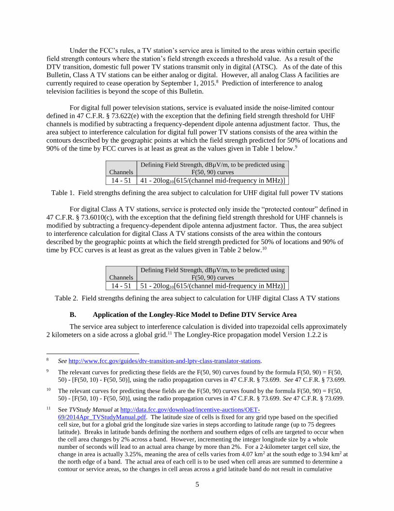
For digital full power television stations, service is evaluated inside the noise-limited contour

defined in 47 C.F.R. § 73.622(e) with the exception that the defining field strength threshold for UHF

channels is modified by subtracting a frequency-dependent dipole antenna adjustment factor. Thus, the

area subject to interference calculation for digital full power TV stations consists of the area within the

contours described by the geographic points at which the field strength predicted for 50% of locations and

90% of the time by FCC curves is at least as great as the values given in Table 1 below.9

Channels

Defining Field Strength, dBµV/m, to be predicted using

F(50, 90) curves

14 - 51 41 - 20log10[615/(channel mid-frequency in MHz)]

Table 1. Field strengths defining the area subject to calculation for UHF digital full power TV stations

For digital Class A TV stations, service is protected only inside the “protected contour” defined in

47 C.F.R. § 73.6010(c), with the exception that the defining field strength threshold for UHF channels is

modified by subtracting a frequency-dependent dipole antenna adjustment factor. Thus, the area subject

to interference calculation for digital Class A TV stations consists of the area within the contours

described by the geographic points at which the field strength predicted for 50% of locations and 90% of

time by FCC curves is at least as great as the values given in Table 2 below.10

Channels

Defining Field Strength, dBµV/m, to be predicted using

F(50, 90) curves

14 - 51 51 - 20log10[615/(channel mid-frequency in MHz)]

Table 2. Field strengths defining the area subject to calculation for UHF digital Class A TV stations

B. Application of the Longley-Rice Model to Define DTV Service Area

The service area subject to interference calculation is divided into trapezoidal cells approximately

2 kilometers on a side across a global grid.11 The Longley-Rice propagation model Version 1.2.2 is

8 See http://www.fcc.gov/guides/dtv-transition-and-lptv-class-translator-stations.

9 The relevant curves for predicting these fields are the F(50, 90) curves found by the formula F(50, 90) = F(50,

50) - [F(50, 10) - F(50, 50)], using the radio propagation curves in 47 C.F.R. § 73.699. See 47 C.F.R. § 73.699.

10 The relevant curves for predicting these fields are the F(50, 90) curves found by the formula F(50, 90) = F(50,

50) - [F(50, 10) - F(50, 50)], using the radio propagation curves in 47 C.F.R. § 73.699. See 47 C.F.R. § 73.699.

11 See TVStudy Manual at http://data.fcc.gov/download/incentive-auctions/OET-

69/2014Apr_TVStudyManual.pdf. The latitude size of cells is fixed for any grid type based on the specified

cell size, but for a global grid the longitude size varies in steps according to latitude range (up to 75 degrees

latitude). Breaks in latitude bands defining the northern and southern edges of cells are targeted to occur when

the cell area changes by 2% across a band. However, incrementing the integer longitude size by a whole

number of seconds will lead to an actual area change by more than 2%. For a 2-kilometer target cell size, the

change in area is actually 3.25%, meaning the area of cells varies from 4.07 km2 at the south edge to 3.94 km2 at

the north edge of a band. The actual area of each cell is to be used when cell areas are summed to determine a

contour or service areas, so the changes in cell areas across a grid latitude band do not result in cumulative

6

applied between the DTV transmitter site and a point in each cell to determine whether the predicted

desired field strength is above the value found in Table 1 or Table 2 for each digital full power or Class A

TV station, respectively, based on the TV station’s operating channel. For cells with population, the point

chosen is the population centroid, as determined using the method implemented in the FCC’s TVStudy

software12 implementing the Longley-Rice model – otherwise the point chosen is the geometric center of

the cell and the point so determined represents the entire cell in all subsequent service and interference

calculations. The station’s directional transmitting antenna patterns (azimuth and elevation), if

applicable, are taken into account in determining the effective radiated power (ERP) in the direction of

each cell.

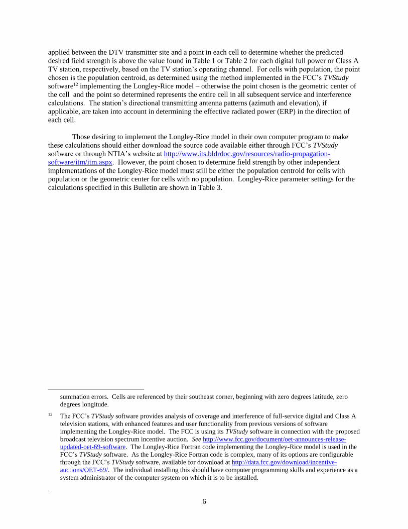
Those desiring to implement the Longley-Rice model in their own computer program to make

these calculations should either download the source code available either through FCC’s TVStudy

software or through NTIA’s website at http://www.its.bldrdoc.gov/resources/radio-propagation-

software/itm/itm.aspx. However, the point chosen to determine field strength by other independent

implementations of the Longley-Rice model must still be either the population centroid for cells with

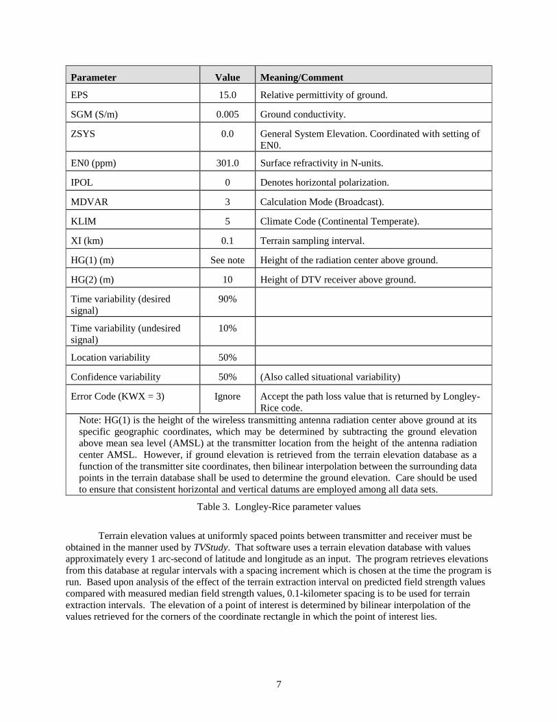
population or the geometric center for cells with no population. Longley-Rice parameter settings for the

calculations specified in this Bulletin are shown in Table 3.

summation errors. Cells are referenced by their southeast corner, beginning with zero degrees latitude, zero

degrees longitude.

12 The FCC’s TVStudy software provides analysis of coverage and interference of full-service digital and Class A

television stations, with enhanced features and user functionality from previous versions of software

implementing the Longley-Rice model. The FCC is using its TVStudy software in connection with the proposed

broadcast television spectrum incentive auction. See http://www.fcc.gov/document/oet-announces-release-

updated-oet-69-software. The Longley-Rice Fortran code implementing the Longley-Rice model is used in the

FCC’s TVStudy software. As the Longley-Rice Fortran code is complex, many of its options are configurable

through the FCC’s TVStudy software, available for download at http://data.fcc.gov/download/incentive-

auctions/OET-69/. The individual installing this should have computer programming skills and experience as a

system administrator of the computer system on which it is to be installed.

.

7

Parameter Value Meaning/Comment

EPS 15.0 Relative permittivity of ground.

SGM (S/m) 0.005 Ground conductivity.

ZSYS 0.0 General System Elevation. Coordinated with setting of

EN0.

EN0 (ppm) 301.0 Surface refractivity in N-units.

IPOL 0 Denotes horizontal polarization.

MDVAR 3 Calculation Mode (Broadcast).

KLIM 5 Climate Code (Continental Temperate).

XI (km) 0.1 Terrain sampling interval.

HG(1) (m) See note Height of the radiation center above ground.

HG(2) (m) 10 Height of DTV receiver above ground.

Time variability (desired

signal)

90%

Time variability (undesired

signal)

10%

Location variability 50%

Confidence variability 50% (Also called situational variability)

Error Code (KWX = 3) Ignore Accept the path loss value that is returned by Longley-

Rice code.

Note: HG(1) is the height of the wireless transmitting antenna radiation center above ground at its

specific geographic coordinates, which may be determined by subtracting the ground elevation

above mean sea level (AMSL) at the transmitter location from the height of the antenna radiation

center AMSL. However, if ground elevation is retrieved from the terrain elevation database as a

function of the transmitter site coordinates, then bilinear interpolation between the surrounding data

points in the terrain database shall be used to determine the ground elevation. Care should be used

to ensure that consistent horizontal and vertical datums are employed among all data sets.

Table 3. Longley-Rice parameter values

Terrain elevation values at uniformly spaced points between transmitter and receiver must be

obtained in the manner used by TVStudy. That software uses a terrain elevation database with values

approximately every 1 arc-second of latitude and longitude as an input. The program retrieves elevations

from this database at regular intervals with a spacing increment which is chosen at the time the program is

run. Based upon analysis of the effect of the terrain extraction interval on predicted field strength values

compared with measured median field strength values, 0.1-kilometer spacing is to be used for terrain

extraction intervals. The elevation of a point of interest is determined by bilinear interpolation of the

values retrieved for the corners of the coordinate rectangle in which the point of interest lies.

8

IV. EVALUATION OF INTERFERENCE

A. Application of the Longley-Rice Model to Determine Interfering Signal Strength

The presence or absence of interference in each grid cell of the area subject to calculation is

determined by further application of the Longley-Rice model. Radio paths between undesired

transmitters and each global 2-kilometer grid point inside the service area are examined. The undesired

transmitters included in the analysis of each cell are those which are possible sources of interference at

that cell, considering their distance from the cell and frequency relationships. For each such radio path,

the Longley-Rice model is applied for median situations (that is, confidence 50%), for 50% of locations,

10% of the time for the prediction of potential interference to TV receivers. In those cases that error code

3 occurs (KWX = 3), the predicted interfering field strength nevertheless is to be accepted in determining

whether there is interference at that location.

B. Areas of Potential Interference

To determine whether the placement of a wireless base station at a particular location would

cause interference to TV receivers, information about each site in a planned wireless base station

deployment is required. Specifically, actual values are required for:

effective radiated power (ERP),

geographic location, and

antenna height above average terrain (HAAT)

The wireless transmit antennas may conservatively be assumed to be non-directional in both the

azimuth and elevation directions, as these may be simpler to implement. However, actual antenna azimuth

and elevation patterns for each planned wireless base station site may be used for increased accuracy by

importing these patterns into the software implementing the Longley-Rice model and setting the azimuth

orientation (N ° E, T) on a site-by-site basis.

The interference analysis for TV reception examines only those cells across the global 2-

kilometer grid within the area subject to calculation that have already been determined to have a desired

field strength above the threshold for reception given in Table 1 or Table 2 as appropriate. A cell on the

global 2-kilometer grid is counted as receiving interference to TV if the ratio of the desired field to that of

the square root of the sum of the squares (root-sum-square, or RSS) of all of an individual wireless

licensee’s undesired wireless interference sources within the appropriate culling distances, defined below,

is less than the minimum D/U threshold value for the corresponding spectral overlap between the TV and

wireless channels. The comparison is made after applying the discrimination effect of the receiving TV

antenna.

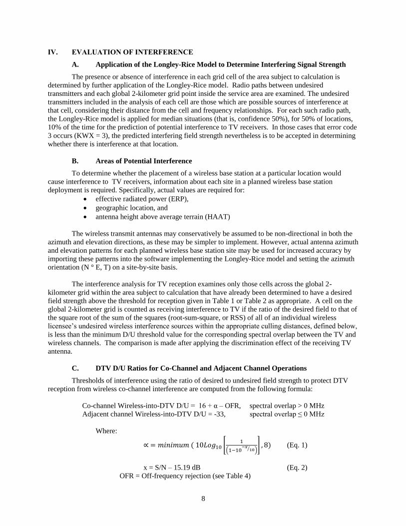
C. DTV D/U Ratios for Co-Channel and Adjacent Channel Operations

Thresholds of interference using the ratio of desired to undesired field strength to protect DTV

reception from wireless co-channel interference are computed from the following formula:

Co-channel Wireless-into-DTV D/U = 16 + α – OFR, spectral overlap > 0 MHz

Adjacent channel Wireless-into-DTV D/U = -33, spectral overlap ≤ 0 MHz

Where:

∝ = 𝑚𝑖𝑛𝑖𝑚𝑢𝑚 ( 10𝐿𝑜𝑔10 [1

(1−10−𝑥

10⁄ )] , 8) (Eq. 1)

x = S/N – 15.19 dB (Eq. 2)

OFR = Off-frequency rejection (see Table 4)

9

The quantity x in Equation 1 is the amount by which the actual desired S/N, computed using Equation 2

below, exceeds the minimum required for DTV reception. As the desired DTV signal level approaches

the minimum level for reception, the D/U ratio will increase exponentially.

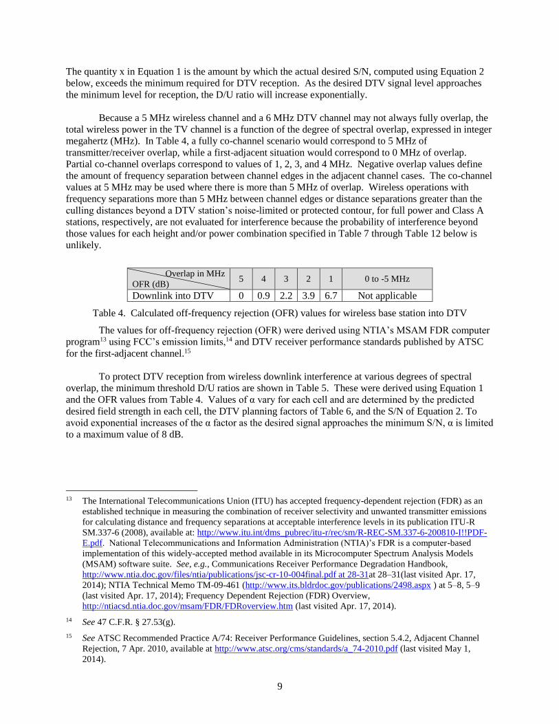
Because a 5 MHz wireless channel and a 6 MHz DTV channel may not always fully overlap, the

total wireless power in the TV channel is a function of the degree of spectral overlap, expressed in integer

megahertz (MHz). In Table 4, a fully co-channel scenario would correspond to 5 MHz of

transmitter/receiver overlap, while a first-adjacent situation would correspond to 0 MHz of overlap.

Partial co-channel overlaps correspond to values of 1, 2, 3, and 4 MHz. Negative overlap values define

the amount of frequency separation between channel edges in the adjacent channel cases. The co-channel

values at 5 MHz may be used where there is more than 5 MHz of overlap. Wireless operations with

frequency separations more than 5 MHz between channel edges or distance separations greater than the

culling distances beyond a DTV station’s noise-limited or protected contour, for full power and Class A

stations, respectively, are not evaluated for interference because the probability of interference beyond

those values for each height and/or power combination specified in Table 7 through Table 12 below is

unlikely.

Overlap in MHz

OFR (dB) 5 4 3 2 1 0 to -5 MHz

Downlink into DTV 0 0.9 2.2 3.9 6.7 Not applicable

Table 4. Calculated off-frequency rejection (OFR) values for wireless base station into DTV

The values for off-frequency rejection (OFR) were derived using NTIA’s MSAM FDR computer

program13 using FCC’s emission limits,14 and DTV receiver performance standards published by ATSC

for the first-adjacent channel.15

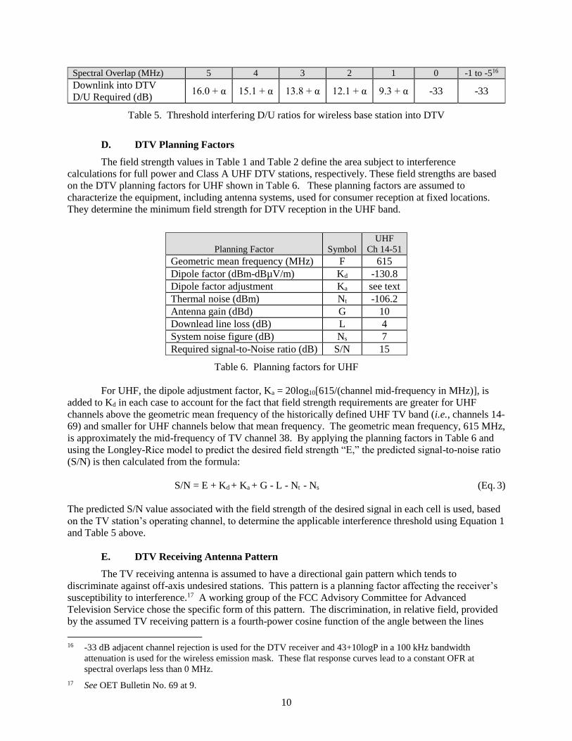
To protect DTV reception from wireless downlink interference at various degrees of spectral

overlap, the minimum threshold D/U ratios are shown in Table 5. These were derived using Equation 1

and the OFR values from Table 4. Values of α vary for each cell and are determined by the predicted

desired field strength in each cell, the DTV planning factors of Table 6, and the S/N of Equation 2. To

avoid exponential increases of the α factor as the desired signal approaches the minimum S/N, α is limited

to a maximum value of 8 dB.

13 The International Telecommunications Union (ITU) has accepted frequency-dependent rejection (FDR) as an

established technique in measuring the combination of receiver selectivity and unwanted transmitter emissions

for calculating distance and frequency separations at acceptable interference levels in its publication ITU-R

SM.337-6 (2008), available at: http://www.itu.int/dms_pubrec/itu-r/rec/sm/R-REC-SM.337-6-200810-I!!PDF-

E.pdf. National Telecommunications and Information Administration (NTIA)’s FDR is a computer-based

implementation of this widely-accepted method available in its Microcomputer Spectrum Analysis Models

(MSAM) software suite. See, e.g., Communications Receiver Performance Degradation Handbook,

http://www.ntia.doc.gov/files/ntia/publications/jsc-cr-10-004final.pdf at 28-31at 28–31(last visited Apr. 17,

2014); NTIA Technical Memo TM-09-461 (http://www.its.bldrdoc.gov/publications/2498.aspx ) at 5–8, 5–9

(last visited Apr. 17, 2014); Frequency Dependent Rejection (FDR) Overview,

http://ntiacsd.ntia.doc.gov/msam/FDR/FDRoverview.htm (last visited Apr. 17, 2014).

14 See 47 C.F.R. § 27.53(g).

15 See ATSC Recommended Practice A/74: Receiver Performance Guidelines, section 5.4.2, Adjacent Channel

Rejection, 7 Apr. 2010, available at http://www.atsc.org/cms/standards/a_74-2010.pdf (last visited May 1,

2014).

10

Spectral Overlap (MHz) 5 4 3 2 1 0 -1 to -516

Downlink into DTV

D/U Required (dB) 16.0 + α 15.1 + α 13.8 + α 12.1 + α 9.3 + α -33 -33

Table 5. Threshold interfering D/U ratios for wireless base station into DTV

D. DTV Planning Factors

The field strength values in Table 1 and Table 2 define the area subject to interference

calculations for full power and Class A UHF DTV stations, respectively. These field strengths are based

on the DTV planning factors for UHF shown in Table 6. These planning factors are assumed to

characterize the equipment, including antenna systems, used for consumer reception at fixed locations.

They determine the minimum field strength for DTV reception in the UHF band.

Planning Factor Symbol

UHF

Ch 14-51

Geometric mean frequency (MHz) F 615

Dipole factor (dBm-dBµV/m) Kd -130.8

Dipole factor adjustment Ka see text

Thermal noise (dBm) Nt -106.2

Antenna gain (dBd) G 10

Downlead line loss (dB) L 4

System noise figure (dB) Ns 7

Required signal-to-Noise ratio (dB) S/N 15

Table 6. Planning factors for UHF

For UHF, the dipole adjustment factor, Ka = 20log10[615/(channel mid-frequency in MHz)], is

added to Kd in each case to account for the fact that field strength requirements are greater for UHF

channels above the geometric mean frequency of the historically defined UHF TV band (i.e., channels 14-

69) and smaller for UHF channels below that mean frequency. The geometric mean frequency, 615 MHz,

is approximately the mid-frequency of TV channel 38. By applying the planning factors in Table 6 and

using the Longley-Rice model to predict the desired field strength “E,” the predicted signal-to-noise ratio

(S/N) is then calculated from the formula:

S/N = E + Kd + Ka + G - L - Nt - Ns (Eq. 3)

The predicted S/N value associated with the field strength of the desired signal in each cell is used, based

on the TV station’s operating channel, to determine the applicable interference threshold using Equation 1

and Table 5 above.

E. DTV Receiving Antenna Pattern

The TV receiving antenna is assumed to have a directional gain pattern which tends to

discriminate against off-axis undesired stations. This pattern is a planning factor affecting the receiver’s

susceptibility to interference.17 A working group of the FCC Advisory Committee for Advanced

Television Service chose the specific form of this pattern. The discrimination, in relative field, provided

by the assumed TV receiving pattern is a fourth-power cosine function of the angle between the lines

16 -33 dB adjacent channel rejection is used for the DTV receiver and 43+10logP in a 100 kHz bandwidth

attenuation is used for the wireless emission mask. These flat response curves lead to a constant OFR at

spectral overlaps less than 0 MHz.

17 See OET Bulletin No. 69 at 9.

11

joining the desired and undesired stations to the reception point. One of these lines goes directly to the

desired station, the other goes to the undesired station. The discrimination is calculated as the fourth

power of the cosine of the angle between these lines but never more than represented by the front-to-back

ratio of 14 dB for UHF. When both desired and undesired stations are on the receive antenna’s boresight,

the angle is 0.0 giving a cosine of unity so that there is no discrimination. When the undesired station is

somewhat off-axis, the cosine will be slightly less than unity and the resulting interference field strength

is reduced accordingly by this value (while the desired field strength remains unchanged); when the

undesired station is far off-axis,18 the maximum discrimination given by the 14 dB front-to-back ratio is

attained, and the resulting interference field strength is reduced by 14 (while the desired field strength still

remains unchanged).

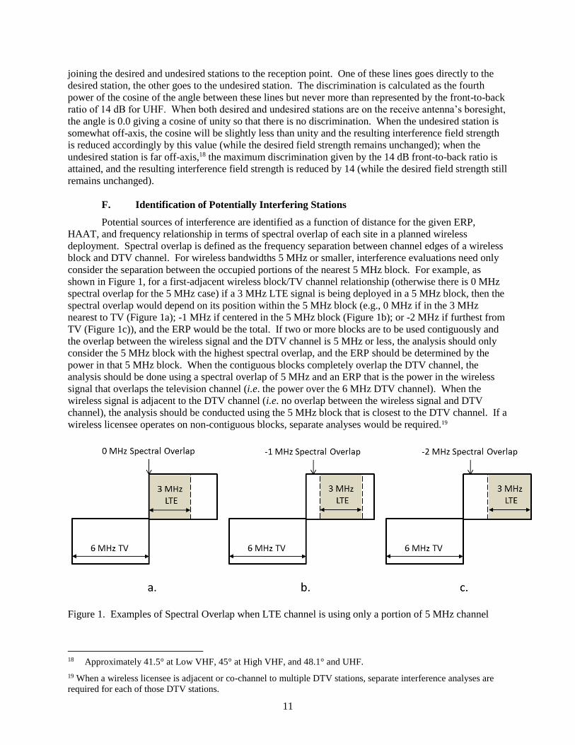
F. Identification of Potentially Interfering Stations

Potential sources of interference are identified as a function of distance for the given ERP,

HAAT, and frequency relationship in terms of spectral overlap of each site in a planned wireless

deployment. Spectral overlap is defined as the frequency separation between channel edges of a wireless

block and DTV channel. For wireless bandwidths 5 MHz or smaller, interference evaluations need only

consider the separation between the occupied portions of the nearest 5 MHz block. For example, as

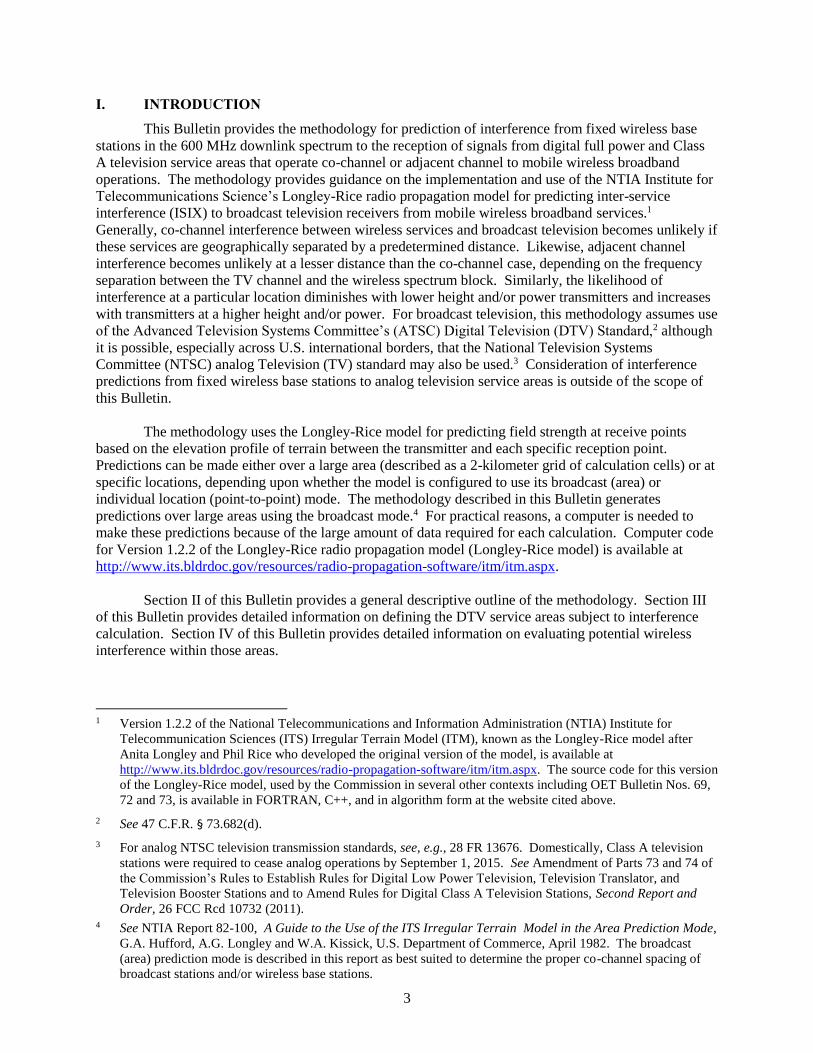
shown in Figure 1, for a first-adjacent wireless block/TV channel relationship (otherwise there is 0 MHz

spectral overlap for the 5 MHz case) if a 3 MHz LTE signal is being deployed in a 5 MHz block, then the

spectral overlap would depend on its position within the 5 MHz block (e.g., 0 MHz if in the 3 MHz

nearest to TV (Figure 1a); -1 MHz if centered in the 5 MHz block (Figure 1b); or -2 MHz if furthest from

TV (Figure 1c)), and the ERP would be the total. If two or more blocks are to be used contiguously and

the overlap between the wireless signal and the DTV channel is 5 MHz or less, the analysis should only

consider the 5 MHz block with the highest spectral overlap, and the ERP should be determined by the

power in that 5 MHz block. When the contiguous blocks completely overlap the DTV channel, the

analysis should be done using a spectral overlap of 5 MHz and an ERP that is the power in the wireless

signal that overlaps the television channel (i.e. the power over the 6 MHz DTV channel). When the

wireless signal is adjacent to the DTV channel (i.e. no overlap between the wireless signal and DTV

channel), the analysis should be conducted using the 5 MHz block that is closest to the DTV channel. If a

wireless licensee operates on non-contiguous blocks, separate analyses would be required.19

Figure 1. Examples of Spectral Overlap when LTE channel is using only a portion of 5 MHz channel

18 Approximately 41.5° at Low VHF, 45° at High VHF, and 48.1° and UHF.

19 When a wireless licensee is adjacent or co-channel to multiple DTV stations, separate interference analyses are

required for each of those DTV stations.

12

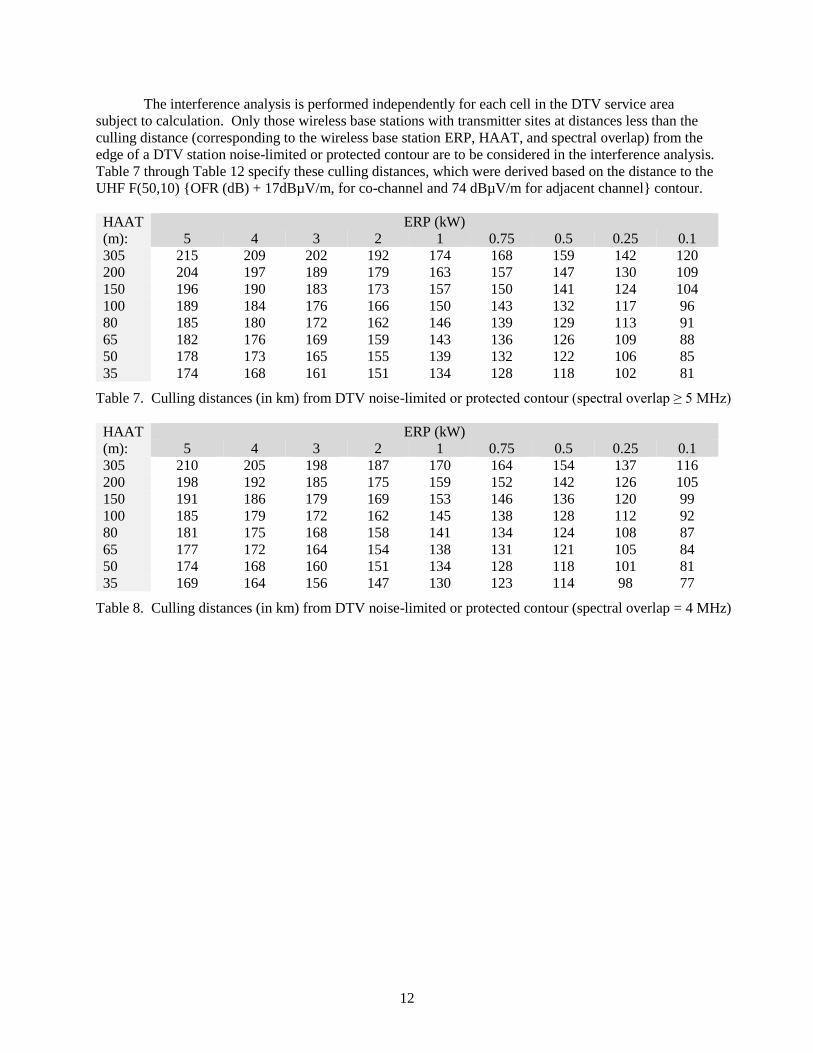
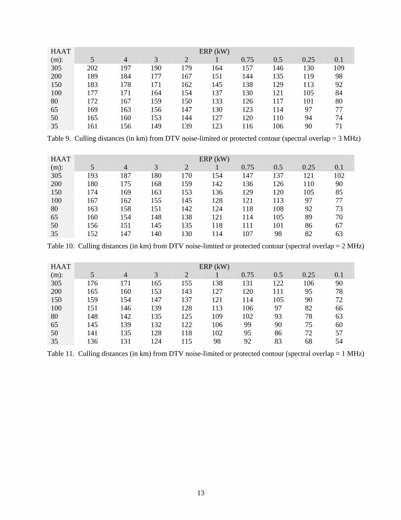
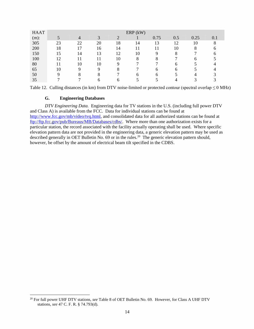
The interference analysis is performed independently for each cell in the DTV service area

subject to calculation. Only those wireless base stations with transmitter sites at distances less than the

culling distance (corresponding to the wireless base station ERP, HAAT, and spectral overlap) from the

edge of a DTV station noise-limited or protected contour are to be considered in the interference analysis.

Table 7 through Table 12 specify these culling distances, which were derived based on the distance to the

UHF F(50,10) {OFR (dB) + 17dBµV/m, for co-channel and 74 dBµV/m for adjacent channel} contour.

HAAT

(m):

ERP (kW)

5 4 3 2 1 0.75 0.5 0.25 0.1

305 215 209 202 192 174 168 159 142 120

200 204 197 189 179 163 157 147 130 109

150 196 190 183 173 157 150 141 124 104

100 189 184 176 166 150 143 132 117 96

80 185 180 172 162 146 139 129 113 91

65 182 176 169 159 143 136 126 109 88

50 178 173 165 155 139 132 122 106 85

35 174 168 161 151 134 128 118 102 81

Table 7. Culling distances (in km) from DTV noise-limited or protected contour (spectral overlap ≥ 5 MHz)

HAAT

(m):

ERP (kW)

5 4 3 2 1 0.75 0.5 0.25 0.1

305 210 205 198 187 170 164 154 137 116

200 198 192 185 175 159 152 142 126 105

150 191 186 179 169 153 146 136 120 99

100 185 179 172 162 145 138 128 112 92

80 181 175 168 158 141 134 124 108 87

65 177 172 164 154 138 131 121 105 84

50 174 168 160 151 134 128 118 101 81

35 169 164 156 147 130 123 114 98 77

Table 8. Culling distances (in km) from DTV noise-limited or protected contour (spectral overlap = 4 MHz)

13

HAAT

(m):

ERP (kW)

5 4 3 2 1 0.75 0.5 0.25 0.1

305 202 197 190 179 164 157 146 130 109

200 189 184 177 167 151 144 135 119 98

150 183 178 171 162 145 138 129 113 92

100 177 171 164 154 137 130 121 105 84

80 172 167 159 150 133 126 117 101 80

65 169 163 156 147 130 123 114 97 77

50 165 160 153 144 127 120 110 94 74

35 161 156 149 139 123 116 106 90 71

Table 9. Culling distances (in km) from DTV noise-limited or protected contour (spectral overlap = 3 MHz)

HAAT

(m):

ERP (kW)

5 4 3 2 1 0.75 0.5 0.25 0.1

305 193 187 180 170 154 147 137 121 102

200 180 175 168 159 142 136 126 110 90

150 174 169 163 153 136 129 120 105 85

100 167 162 155 145 128 121 113 97 77

80 163 158 151 142 124 118 108 92 73

65 160 154 148 138 121 114 105 89 70

50 156 151 145 135 118 111 101 86 67

35 152 147 140 130 114 107 98 82 63

Table 10. Culling distances (in km) from DTV noise-limited or protected contour (spectral overlap = 2 MHz)

HAAT

(m):

ERP (kW)

5 4 3 2 1 0.75 0.5 0.25 0.1

305 176 171 165 155 138 131 122 106 90

200 165 160 153 143 127 120 111 95 78

150 159 154 147 137 121 114 105 90 72

100 151 146 139 128 113 106 97 82 66

80 148 142 135 125 109 102 93 78 63

65 145 139 132 122 106 99 90 75 60

50 141 135 128 118 102 95 86 72 57

35 136 131 124 115 98 92 83 68 54

Table 11. Culling distances (in km) from DTV noise-limited or protected contour (spectral overlap = 1 MHz)

14

HAAT

(m):

ERP (kW)

5 4 3 2 1 0.75 0.5 0.25 0.1

305 23 22 20 18 14 13 12 10 8

200 18 17 16 14 11 11 10 8 6

150 15 14 13 12 10 9 8 7 6

100 12 11 11 10 8 8 7 6 5

80 11 10 10 9 7 7 6 5 4

65 10 9 9 8 7 6 6 5 4

50 9 8 8 7 6 6 5 4 3

35 7 7 6 6 5 5 4 3 3

Table 12. Culling distances (in km) from DTV noise-limited or protected contour (spectral overlap ≤ 0 MHz)

G. Engineering Databases

DTV Engineering Data. Engineering data for TV stations in the U.S. (including full power DTV

and Class A) is available from the FCC. Data for individual stations can be found at

http://www.fcc.gov/mb/video/tvq.html, and consolidated data for all authorized stations can be found at

ftp://ftp.fcc.gov/pub/Bureaus/MB/Databases/cdbs/. Where more than one authorization exists for a

particular station, the record associated with the facility actually operating shall be used. Where specific

elevation pattern data are not provided in the engineering data, a generic elevation pattern may be used as

described generally in OET Bulletin No. 69 or in the rules.20 The generic elevation pattern should,

however, be offset by the amount of electrical beam tilt specified in the CDBS.

20 For full power UHF DTV stations, see Table 8 of OET Bulletin No. 69. However, for Class A UHF DTV

stations, see 47 C. F. R. § 74.793(d).