FEA Information Engineering Journal - April 2012.pdf - feaiej

ISSN 2167-1273 Volume 1

Issue 3 April 2012

FEA Information Engineering Journal

FLUID STRUCTURE INTERACTION

2 Fea Information Engineering Journal April 2012


Aim and Scope FEA Information Engineering Journal (FEAIEJ™) is a monthly published online journal to cover the latest Finite Element Analysis Technologies. The journal aims to cover previous noteworthy published papers and original papers. All published papers are peer reviewed in the respective FEA engineering fields. Consideration is given to all aspects of technically excellent written information without limitation on length. All submissions must follow guidelines for publishing a paper, or periodical. If a paper has been previously published, FEAIEJ requires written permission to reprint, with the proper acknowledgement give to the publisher of the published work. Reproduction in whole, or part, without the express written permissio of FEA Information Engineering Journal, or the owner of of the copyright work, is strictly prohibited. FEAIJ welcomes unsolicited topics, ideas, and articles. Monthly publication is limited to no more then five papers, either reprint, or original. Papers will be archived on www.feaiej.com For information on publishing a paper original or reprint contact [email protected] Subject line: Journal Publication

Cover: FSI problem of a opening valve and the flow is shown and maximum aperture when the flow rate peaks. The turbulence was modeled using a LES approach. Advances on the Incompressible CFD Solver in LS-DYNA® - Facundo Del Pin, LSTC.

http://www.feaiej.com/

mailto:[email protected]

3 Fea Information Engineering Journal April 2012


TABLE OF CONTENTS

Volume 1, Issue No. 3 April 2012 Reprint from the 11th International LS-DYNA® Users Conference 2010, June 6-8, 2010 held in Dearborn, MI, USA April issue is dedication to Fluid Structure Interaction (FSI) Advances on the Incompressible CFD Solver in LS-DYNA® Del Pin, F. How To Use the New CESE Compressible Fluid Solver in LS-DYNA® Zhang, Z.C. ALE Incompressible Fluid in LS-DYNA® Souli, M. Module Development of Multiphase and Chemically Reacting Flow in LS-DYNA® Compressible Flow Solver Im, K.S, Zhang, Z.C., Cook, G. All contents are copyright © to the publishing company, author or respective company. All rights

reserved.

11th International LS-DYNA® Users Conference Fluid / FSI

6-1

Advances on the Incompressible CFD Solver in LS-DYNA®

Facundo Del Pin Livermore Software Technology Corporation

Abstract The present work will introduce some of the resent developments in the Incompressible CFD (ICFD) solver currently under development in LS-DYNA. The main feature of this solver is its ability to couple with any solid model to perform Fluid-Structure interaction (FSI) analysis. Highly non-linear behavior is supported by using automatic re-meshing strategies to maintain element quality within acceptable limits. In this work we will introduce the additional features for conjugate heat transfer, turbulence model, biphasic flow, some new feature in terms of mesh generation like boundary layer meshing and MPP.

Introduction Incompressible flows cover a vast number of engineering problems ranging from car aerodynamics to arterial flows and parachute simulation. As a rule of thumb a flow may be considered incompressible if the Mach number presented in any part of the domain is not larger than 0.3. In LS-DYNA there are other two options to do CFD depending upon the kind of problem. The CESE solver is highly accurate CFD solver for compressible fluids. The ALE solver has support for both compressible and incompressible and it is a good option for highly transient problems. Due to the requirement of industrial applications a number of new features have been added to the ICFD solver prior to the release version. They will be briefly described bellow.

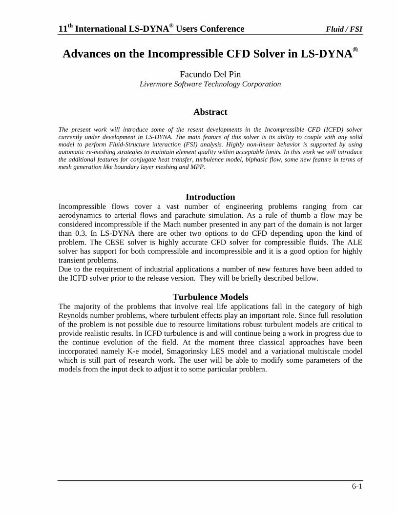
Turbulence Models The majority of the problems that involve real life applications fall in the category of high Reynolds number problems, where turbulent effects play an important role. Since full resolution of the problem is not possible due to resource limitations robust turbulent models are critical to provide realistic results. In ICFD turbulence is and will continue being a work in progress due to the continue evolution of the field. At the moment three classical approaches have been incorporated namely K-e model, Smagorinsky LES model and a variational multiscale model which is still part of research work. The user will be able to modify some parameters of the models from the input deck to adjust it to some particular problem.

Fluid / FSI 11th International LS-DYNA® Users Conference

6-2

Figure 1: the image shows a flow past a flat plate in an angle on the left, simulating the wind effect on a solar panel. The image on the right is an FSI problem of a opening valve and the flow is shown and maximum aperture when the flow rate peaks. In both cases the turbulence was modeled using a LES approach.

Conjugate Heat Transfer

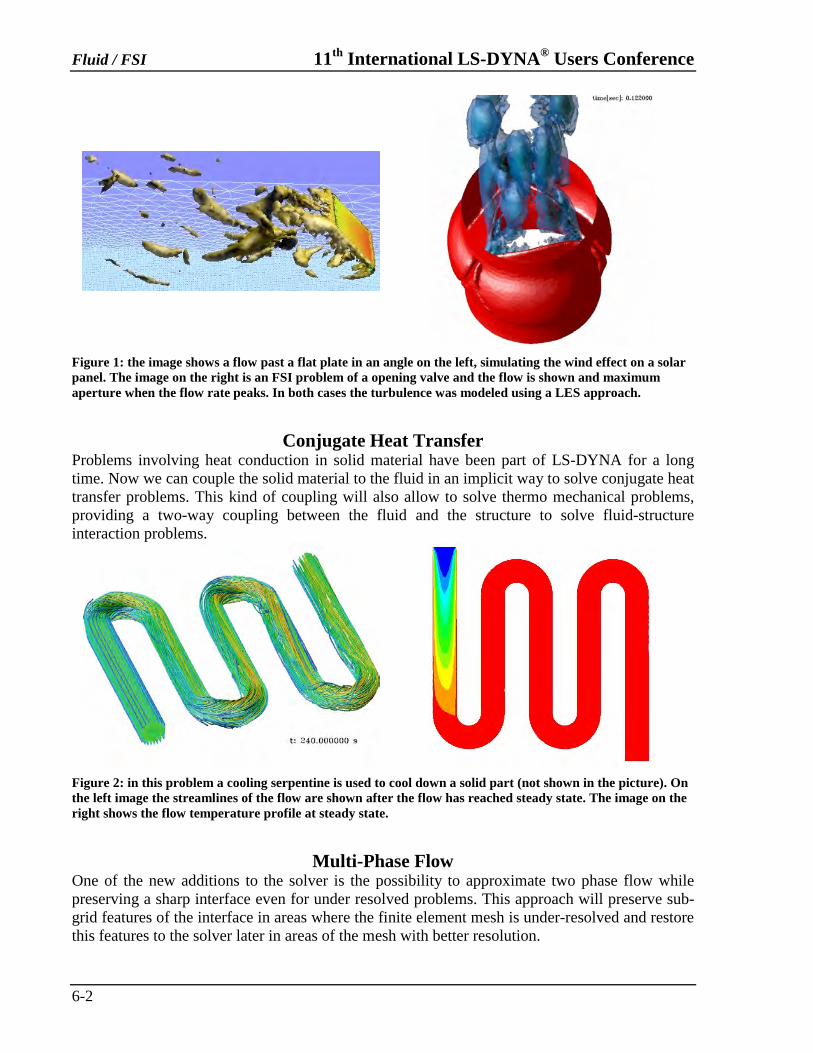
Problems involving heat conduction in solid material have been part of LS-DYNA for a long time. Now we can couple the solid material to the fluid in an implicit way to solve conjugate heat transfer problems. This kind of coupling will also allow to solve thermo mechanical problems, providing a two-way coupling between the fluid and the structure to solve fluid-structure interaction problems.

Figure 2: in this problem a cooling serpentine is used to cool down a solid part (not shown in the picture). On the left image the streamlines of the flow are shown after the flow has reached steady state. The image on the right shows the flow temperature profile at steady state.

Multi-Phase Flow

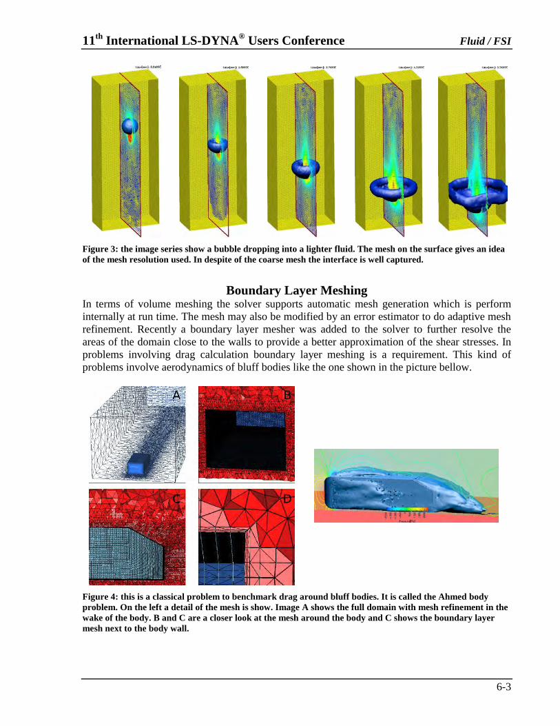
One of the new additions to the solver is the possibility to approximate two phase flow while preserving a sharp interface even for under resolved problems. This approach will preserve sub-grid features of the interface in areas where the finite element mesh is under-resolved and restore this features to the solver later in areas of the mesh with better resolution.


6-3

Figure 3: the image series show a bubble dropping into a lighter fluid. The mesh on the surface gives an idea of the mesh resolution used. In despite of the coarse mesh the interface is well captured.

Boundary Layer Meshing

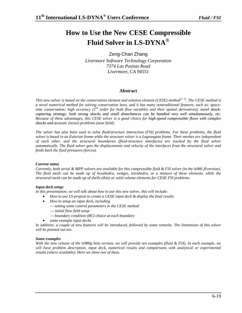
In terms of volume meshing the solver supports automatic mesh generation which is perform internally at run time. The mesh may also be modified by an error estimator to do adaptive mesh refinement. Recently a boundary layer mesher was added to the solver to further resolve the areas of the domain close to the walls to provide a better approximation of the shear stresses. In problems involving drag calculation boundary layer meshing is a requirement. This kind of problems involve aerodynamics of bluff bodies like the one shown in the picture bellow.

Figure 4: this is a classical problem to benchmark drag around bluff bodies. It is called the Ahmed body problem. On the left a detail of the mesh is show. Image A shows the full domain with mesh refinement in the wake of the body. B and C are a closer look at the mesh around the body and C shows the boundary layer mesh next to the body wall.


6-4

Parallel Computing To improve the productivity of the solver and to satisfy the demand for high performance computing all the features of the solver have been implemented in parallel. The parallel CFD solver can be coupled to the parallel solid mechanics solver to do parallel FSI. In the same way the coupling may be done in parallel with the thermal solver to do conjugate heat transfer.


6-19

How to Use the New CESE Compressible Fluid Solver in LS-DYNA®

Zeng-Chan Zhang Livermore Software Technology Corporation

7374 Las Positas Road Livermore, CA 94551

Abstract This new solver is based on the conservation element and solution element (CESE) method[1, 2]. The CESE method is a novel numerical method for solving conservation laws, and it has many nontraditional features, such as: space-time conservation; high accuracy (2nd order for both flow variables and their spatial derivatives); noovveell sshhoocckk--ccaappttuurriinngg ssttrraatteeggyy; bootthh ssttrroonngg sshhoocckkss aanndd ssmmaallll ddiissttuurrbbaanncceess ccaann bbee hhaannddlleedd vveerryy wweellll ssiimmuullttaanneeoouussllyy,, eettcc.. Because of these advantages, this CESE solver is a good choice for hhiigghh--ssppeeeedd ccoommpprreessssiibbllee fflloowwss wwiitthh ccoommpplleexx sshhoocckkss aanndd aacoustic (noise) problems (near field). The solver has also been used to solve fluid/structure interaction (FSI) problems. For these problems, the fluid solver is based in an Eulerian frame while the structure solver is a Lagrangian frame. Their meshes are independent of each other, and the structural boundaries (fluid-structure interfaces) are tracked by the fluid solver automatically. The fluid solver gets the displacements and velocity of the interfaces from the structural solver and feeds back the fluid pressures (forces). Current status Currently, both serial & MPP solvers are available for this compressible fluid & FSI solver (in the ls980 β-version). The fluid mesh can be made up of hexahedra, wedges, tetrahedra, or a mixture of these elements, while the structural mesh can be made up of shells (thin) or solid volume elements for CESE FSI problems. Input deck setup: In this presentation, we will talk about how to use this new solver, this will include:

• How to use LS-prepost to create a CESE input deck & display the final results • How to setup an input deck, including

⎯ setting some control parameters in the CESE method ⎯ initial flow field setup ⎯ boundary condition (BC) choice at each boundary

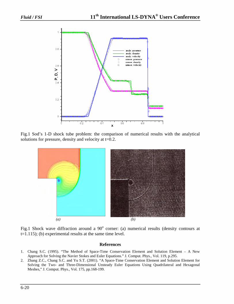
• some example input decks In addition, a couple of new features will be introduced, followed by some remarks. The limitations of this solver will be pointed out too. Some examples With the new release of the ls980g beta version, we will provide ten examples (fluid & FSI). In each example, we will have problem description, input deck, numerical results and comparisons with analytical or experimental results (where available). Here we show two of them.


6-20

Fig.1 Sod’s 1-D shock tube problem: the comparison of numerical results with the analytical solutions for pressure, density and velocity at t=0.2.

(a) (b) Fig.1 Shock wave diffraction around a 90o corner: (a) numerical results (density contours at t=1.115); (b) experimental results at the same time level.

References

1. Chang S.C. (1995). “The Method of Space-Time Conservation Element and Solution Element – A New Approach for Solving the Navier Stokes and Euler Equations.” J. Comput. Phys., Vol. 119, p.295.

2. Zhang Z.C., Chang S.C. and Yu S.T. (2001). “A Space-Time Conservation Element and Solution Element for Solving the Two- and Three-Dimensional Unsteady Euler Equations Using Quadrilateral and Hexagonal Meshes,” J. Comput. Phys., Vol. 175, pp.168-199.


6-29

ALE Incompressible Fluid in LS-DYNA®

Mhamed Souli University of Lille, France

Abstract The computation of fluid forces acting on a rigid or deformable structure constitutes a major problem in fluid-structure interaction. However, the majority of numerical tests consists in using two different codes to separately solve pressure of the fluid and structural displacements. In this paper, a monolithic with an ALE formulation approach is used to implicitly calculate the pressure of an incompressible fluid applied to the structure. The projection method proposed by Gresho is used to decouple the velocity and pressure

Introduction

A computational procedure is developed to solve problems of viscous incompressible flows interacting with rigid or deformable structure. The arbitrary Lagrangian Eulerian method (ALE) is used to move the internal fluid nodes whereas the boundary fluid nodes move with the structure. The coupling of the mesh motion equations and the fluid equations is essentially done through contact surface boundary conditions. In continuum Mechanics, two descriptions are considered for the motion in a continuum media

ALE Description The ALE description for incompressible viscous flows has been developed by Hughes at al [1], to solve free surface flows and fluid-structure interaction problems. The general kinematics theory developed in [1] serves as the basis of the Lagrangian-Eulerian description. For this purpose, the authors define three domains in space, and mappings from one domain to the other. The first one, called the spatial domain, is considered as the domain on which the fluid problem is posed. The spatial domain is generally in motion, because of moving boundaries. The second domain, called the material domain, is to be thought of as the domain occupied at time t=0 by the material particles which occupy the spatial domain at time t. The third domain, called the reference domain, is defined as a fixed domain throughout. From these domain descriptions, we can see that the Eulerian description is obtained when the spatial domain coincides with the reference domain, whereas the Lagrangian reference is obtained when the material domain coincides with the reference domain. Both the material and spatial domains are generally in motion with respect to the reference domain; it is convenient to express the material time derivative of a physical property φ in the reference configuration.

φφφ ∇+= .,

.

ct (1)

where .

φ is the material time derivative, and t,φ is the time derivative when freezing coordinates

in the reference domain, c is the convective velocity. meshvvc −= (2)


6-30

v is the fluid velocity, and meshv is the mesh velocity. In the Eulerian description, the mesh velocity is zero, 0=meshv , whereas in the Lagrangian description vvmesh = , and .0=c In the ALE formulation, the mesh nodes move with an arbitrary velocity. The choice of the mesh velocity constitutes one of the major problems with the ALE description. Different techniques have been developed for updating the mesh in a fluid motion, depending on the fluid domain. For problems defined in simple domains, the mesh velocity can be deduced through a uniform or non uniform distribution of the nodes along straight lines ending at the moving boundaries.

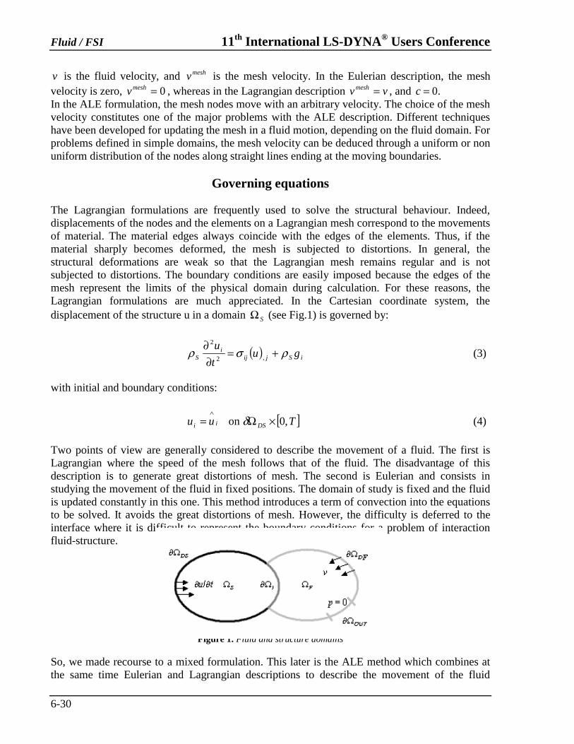
Governing equations The Lagrangian formulations are frequently used to solve the structural behaviour. Indeed, displacements of the nodes and the elements on a Lagrangian mesh correspond to the movements of material. The material edges always coincide with the edges of the elements. Thus, if the material sharply becomes deformed, the mesh is subjected to distortions. In general, the structural deformations are weak so that the Lagrangian mesh remains regular and is not subjected to distortions. The boundary conditions are easily imposed because the edges of the mesh represent the limits of the physical domain during calculation. For these reasons, the Lagrangian formulations are much appreciated. In the Cartesian coordinate system, the displacement of the structure u in a domain SΩ (see Fig.1) is governed by:

( ) iSjiji

S gut

u ρσρ +=∂∂

,2

2

(3)

with initial and boundary conditions:

[ ]Tuu DSii ,0on ×Ω=∧

δ (4)

Two points of view are generally considered to describe the movement of a fluid. The first is Lagrangian where the speed of the mesh follows that of the fluid. The disadvantage of this description is to generate great distortions of mesh. The second is Eulerian and consists in studying the movement of the fluid in fixed positions. The domain of study is fixed and the fluid is updated constantly in this one. This method introduces a term of convection into the equations to be solved. It avoids the great distortions of mesh. However, the difficulty is deferred to the interface where it is difficult to represent the boundary conditions for a problem of interaction fluid-structure.

Figure 1. Fluid and structure domains

So, we made recourse to a mixed formulation. This later is the ALE method which combines at the same time Eulerian and Lagrangian descriptions to describe the movement of the fluid


6-31

particles. In this framework, the velocity of the incompressible viscous fluid in a domain is characterized by the mass and momentum conservation laws such that:

[ ]Tv Fii ,0in0, ×Ω= (5)

( ) [ ]Tgvvvt

vFijij

Fji

mjj

i ,0in1

,, ×Ω=−−+∂∂ τ

ρ (6)

where iv and fρ indicate, respectively, the flow velocity components and the fluid density. The

term mjv represents the velocity of the mesh. If 0=m

jv , we obtain the Eulerian formulation

because the convective velocity of the mesh is null. If jmj vv = , we obtain the Lagrangian

formulation for which the convective velocity is the fluid velocity. The quantity mjj vv − is the

relative velocity and the stress tensor ijτ is commonly defined by:

( ) ijijjiFij pvv δμτ −+= ,, (7)

where Fμ is the fluid dynamic viscosity. The momentum equation is to be solved with the initial condition and the boundary conditions:

( ) Fiv Ω= in00 (8)

[ ]Tvv DFii ,0on ×Ω=∧

δ (9)

where iv∧

are the imposed velocity components on DFΩδ .

The boundary conditions on the fluid-structure interface IΩδ are given by :

[ ]Tt

uv I

ii ,0on ×Ω

∂∂

= δ (10)

And 0=p , on the outflow boundary

Fluid Analysis Algorithm It is well known that the main difficulties arising in the numerical solution of the convection-diffusion equations are due to their no-self-adjoint character. The standard Galerkin method leads to no physical spatial oscillations when applied to the high convective case. To preclude such anomalies, the most popular method being the use of upwind differencing on the convective term via Petrov-Galerkin methods (see, for example, Heinrich & al [2]; Heinrich and Zienkiewicz [3], Belytscho & al. [4]). Although theses methods are precise and stable, we will use a ‘split’ method which is a simple mean to obtain a robust and effective formulation. This time-split method decomposes the time step into two phases : – Phase 1 is a solution of the Lagrangian equations of motion (advection terms are nil) updating the velocity field by the effects of all forces. For the fluid, the velocity-pressure formulation of the discretized problem is decoupled by the projection method (for more details, see Cho and Lee [5]).


6-32

– Phase 2 adds advection contributions, and is required for runs that are Eulerian or contain some relative motion of mesh and fluid. In order to effectively solve the pressure and velocities satisfying the continuity constraint Eq.(5) for the phase 1, we adopt the fractional method proposed by Gresho [6]. The idea of these methods is to decouple the velocity v and the pressure p. These are based on a resolution in three steps of the Navier-Stokes equations. Hereafter, we describe briefly the above method in Lagrangian formulation:

– Intermediate velocity. The first step consists in calculating an intermediate velocity ∗iv ,

solution of the Naviers-Stokes equation without taking into account the continuity constraint.

Fni

ni

F

njji

F

Fni

ni gpvtvv Ω⎟⎟

⎠

⎞⎜⎜⎝

⎛+−Δ+=

+in

1,,

1*

ρρμ (11)

I

nin

i t

uv Ω∂

∂∂

=+on

1* (12)

– Projection. As the velocity ∗iv does not yet satisfy the incompressibility condition Eq.(5), it is

projected on a divergence free space to get an adequate approximation of the velocity. This is obtained from :

iF

ii pt

vv ,* ΔΔ+=

ρ (13)

with 01, =+niiv . The term pΔ is a pressure increment.

The second step consists in deriving a Poisson equation for the pressure p. In fact, by taking the divergence of Eq.(13) and using the incompressibility condition Eq.(5), we obtain :

F

n

iinii

F

vt

p ΩΔ

=Δ ++ in11 1*

,1

,ρ (14)

Once the corrective pressure 1+Δ np has been determined, the final velocity field is obtained from

the intermediate velocity ∗iv and 1+Δ np :

Fni

F

n

ini p

tvv ΩΔΔ−= ++∗+ in1

,

11

ρ (15)

– Pressure update. Since v is the physical velocity, the pressure p can be given from 1+Δ np .

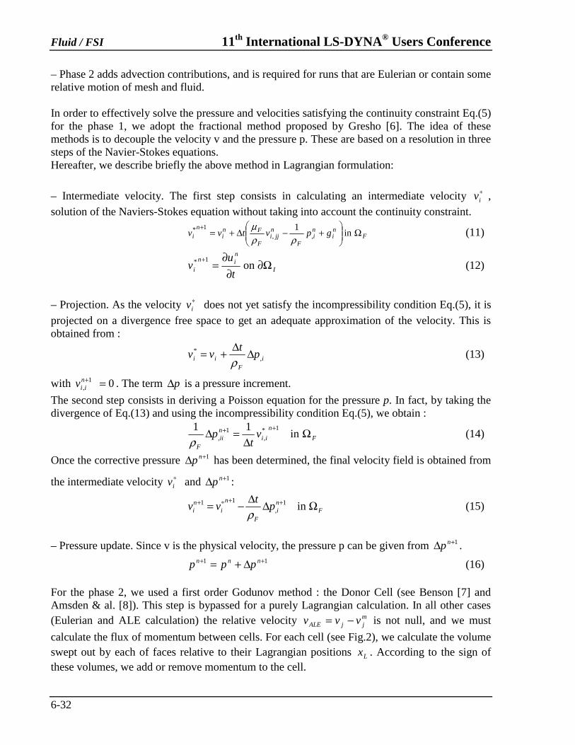
11 ++ Δ+= nnn ppp (16) For the phase 2, we used a first order Godunov method : the Donor Cell (see Benson [7] and Amsden & al. [8]). This step is bypassed for a purely Lagrangian calculation. In all other cases (Eulerian and ALE calculation) the relative velocity m

jjALE vvv −= is not null, and we must

calculate the flux of momentum between cells. For each cell (see Fig.2), we calculate the volume swept out by each of faces relative to their Lagrangian positions Lx . According to the sign of these volumes, we add or remove momentum to the cell.


6-33

Figure 2. Advected volume

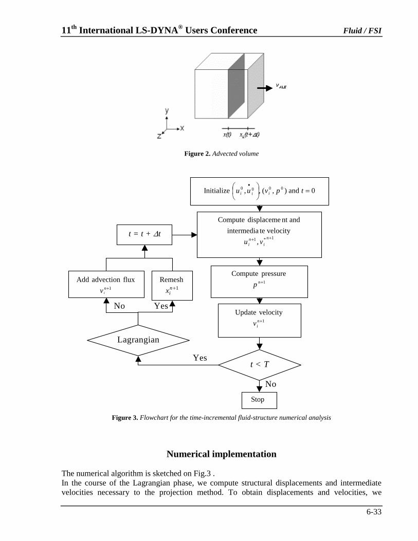
Figure 3. Flowchart for the time-incremental fluid-structure numerical analysis

Numerical implementation The numerical algorithm is sketched on Fig.3 . In the course of the Lagrangian phase, we compute structural displacements and intermediate velocities necessary to the projection method. To obtain displacements and velocities, we

0and),(,,Initialize 0000 =⎟

⎠⎞

⎜⎝⎛ •

tpvuu iii

1*1 ,

velocityteintermedia

andnt displaceme Compute

++ n

ini vu

1

pressureCompute+np

1

velocityUpdate+n

iv

Stop

1

Remesh+n

ix1

fluxadvection Add+n

iv

t = t + Δt

Lagrangiann

t < T

Yes No

Yes

No


6-34

compute nodal forces from respectively Eq.(11) and Eq.(12). This allows us to use the same method to solve the structural behaviour and the liquid dynamic response. The difference between the structural algorithm and the fluid algorithm is the computation of stress tensors. Then, we solve the pressure from Eq.(14) and Eq.(16). So, we obtain the velocity which is solenoidal (div(v) = 0). For the Lagrangian nodes, we move the domain to update the coordinates of the nodes. And for the other nodes, we compute the momentum flux of the cell in order to update the velocity.

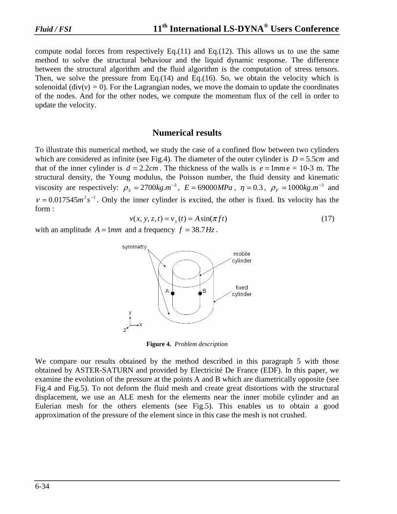
Numerical results To illustrate this numerical method, we study the case of a confined flow between two cylinders which are considered as infinite (see Fig.4). The diameter of the outer cylinder is cmD 5.5= and that of the inner cylinder is cmd 2.2= . The thickness of the walls is mme 1= e = 10-3 m. The structural density, the Young modulus, the Poisson number, the fluid density and kinematic viscosity are respectively: 3.2700 −= mkgSρ , MPaE 69000= , 3.0=η , 3.1000 −= mkgFρ and

12017545.0 −= smν . Only the inner cylinder is excited, the other is fixed. Its velocity has the form :

)sin()(),,,( tfAtvtzyxv x π== (17)

with an amplitude mmA 1= and a frequency Hzf 7.38= .

Figure 4. Problem description

We compare our results obtained by the method described in this paragraph 5 with those obtained by ASTER-SATURN and provided by Electricité De France (EDF). In this paper, we examine the evolution of the pressure at the points A and B which are diametrically opposite (see Fig.4 and Fig.5). To not deform the fluid mesh and create great distortions with the structural displacement, we use an ALE mesh for the elements near the inner mobile cylinder and an Eulerian mesh for the others elements (see Fig.5). This enables us to obtain a good approximation of the pressure of the element since in this case the mesh is not crushed.


6-35

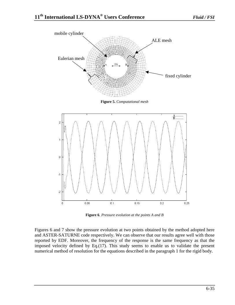
Figure 5. Computational mesh

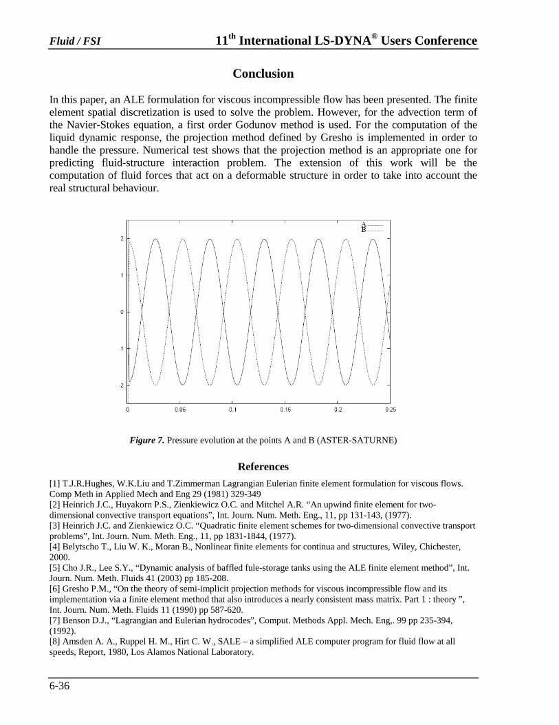
Figure 6. Pressure evolution at the points A and B

Figures 6 and 7 show the pressure evolution at two points obtained by the method adopted here and ASTER-SATURNE code respectively. We can observe that our results agree well with those reported by EDF. Moreover, the frequency of the response is the same frequency as that the imposed velocity defined by Eq.(17). This study seems to enable us to validate the present numerical method of resolution for the equations described in the paragraph 1 for the rigid body.

Eulerian mesh

ALE mesh

fixed cylinder

mobile cylinder


6-36

Conclusion In this paper, an ALE formulation for viscous incompressible flow has been presented. The finite element spatial discretization is used to solve the problem. However, for the advection term of the Navier-Stokes equation, a first order Godunov method is used. For the computation of the liquid dynamic response, the projection method defined by Gresho is implemented in order to handle the pressure. Numerical test shows that the projection method is an appropriate one for predicting fluid-structure interaction problem. The extension of this work will be the computation of fluid forces that act on a deformable structure in order to take into account the real structural behaviour.

Figure 7. Pressure evolution at the points A and B (ASTER-SATURNE)

References

[1] T.J.R.Hughes, W.K.Liu and T.Zimmerman Lagrangian Eulerian finite element formulation for viscous flows. Comp Meth in Applied Mech and Eng 29 (1981) 329-349 [2] Heinrich J.C., Huyakorn P.S., Zienkiewicz O.C. and Mitchel A.R. “An upwind finite element for two-dimensional convective transport equations”, Int. Journ. Num. Meth. Eng., 11, pp 131-143, (1977). [3] Heinrich J.C. and Zienkiewicz O.C. “Quadratic finite element schemes for two-dimensional convective transport problems”, Int. Journ. Num. Meth. Eng., 11, pp 1831-1844, (1977). [4] Belytscho T., Liu W. K., Moran B., Nonlinear finite elements for continua and structures, Wiley, Chichester, 2000. [5] Cho J.R., Lee S.Y., “Dynamic analysis of baffled fule-storage tanks using the ALE finite element method”, Int. Journ. Num. Meth. Fluids 41 (2003) pp 185-208. [6] Gresho P.M., “On the theory of semi-implicit projection methods for viscous incompressible flow and its implementation via a finite element method that also introduces a nearly consistent mass matrix. Part 1 : theory ”, Int. Journ. Num. Meth. Fluids 11 (1990) pp 587-620. [7] Benson D.J., “Lagrangian and Eulerian hydrocodes”, Comput. Methods Appl. Mech. Eng,. 99 pp 235-394, (1992). [8] Amsden A. A., Ruppel H. M., Hirt C. W., SALE – a simplified ALE computer program for fluid flow at all speeds, Report, 1980, Los Alamos National Laboratory.


6-37

Module Development of Multiphase and Chemically Reacting Flow in LS-DYNA® Compressible Flow Solver

Kyoung-Su Im, Zeng-Chan Zhang, and Grant Cook, Jr.

Livermore Software Technology Corp. Livermore, CA 94551, USA

Abstract

We reported a significant progress of the simulation module developments such as the cavitation, supersonic heterogeneous combustion, and gaseous detonations for the compressible flow solver. The homogeneous equilibrium model (HEM) based on the acoustic speed of the mixture of liquid and vapor was implemented for automotive diesel injectors, where the cavitation effects should correctly predict for the nozzle design. The heterogeneous combustion based on an Eulerian-Lagrangian model was developed for thermobaric explosive (TBX) applications in which a stochastic particle technique in conjunction with a probability density function (PDF) is adopted. In modeling of gaseous detonation, we implemented various combustion modules depending on the reaction model: one-step reaction (ZND model), reduced reaction of intrinsic low-dimensional manifolds (ILDM), and detailed chemistry model. Application results validated with experimental data are demonstrated with detailed discussion.

Introduction

The numerical simulation of cavitating nozzle flows in high-pressure, high-speed diesel injectors has become a more widely interesting topic because the cavitation phenomenon inside a fuel injector can provide valuable and detailed information for nozzle design and spray breakup modeling. However, the numerical simulation of the cavitating flows is a difficult stiff problem accompanied from a multiphase phenomenon between liquid and gas phase. In general, there are two ways to resolve the problem. The first one is to construct an equation of state (EOS) valid for the liquid, the mixture, and the gas phase. Such a type of approach is well-posedness if one can provide a valid EOS for the mixture phase. The other is to use the non-equilibrium multiphase flow model. With this model, each phase has its own EOS and the gas phase typically by an ideal gas EOS. Many studies have tried to predict complex cavitating flows by numerical methods [1-3]. Among the existing methods, we applied Schmidt’s homogeneous equilibrium model (HEM)[3], which is based on the acoustic speed of the mixture of liquid and vapor. This model is simple but contains the important characteristic information of cavitating flows. More specifically, for present diesel injection systems like a small geometry (180 µm of nozzle diameter) and very high velocities (driven by 1000-bar injection pressure through the nozzle), the continuum model considering the compressibility of the liquid and vapor should be able to correctly predict the cavitaing effects from two different nozzle geometries, which would be able to more clearly understand the near nozzle breakup and sprays.

Heterogeneous combustion (i. e, solid and gas or liquid and gas) has a wide range of applications such as solid rocket propulsion, controlling the combustion instability, underwater explosion, and high energy explosion [4-6]. Among several possible combinations, a thermobaric explosive (TBX) composed of trinitrotoluene (TNT) and energetic metal particles (typically aluminum) is a widely used explosive and is of great importance in the safety, mining, and defense industries. After the onset of the detonation developed from the initial burst charge, TBX is typically accompanied by a secondary combustion, or afterburning, which releases more energy than the initial bursting charge explosion so that a fairly large combustion area within the fireball radius is sustained until all combustion products are consumed [7].


6-38

In general, there are three experimental methods to initiate detonation: (i) flame initiation, (ii) shock wave initiation, and (iii) direct initiation. In all three cases, shock waves occur prior to detonation initiation. The present paper demonstrates on the third initiation mode, which is relevant to the detonation initiation process in a pulse detonation engine (PDE). In this mode [8-10], a large amount of energy is instantaneously deposited to a small region of unconfined combustible mixture. Immediately, a strong blast wave is generated. This spherical (or cylindrical) shock wave expands and decays while it continues heating the gas mixture. Due to shock heating, chemical reactions occur and chemical energy is released. Under suitable conditions, detonation is initiated. The blast wave generated by igniter plays an important role because it produces the critical states for the onset of the detonation. For the present demonstration, three initiation energies are used for the supercritical, the sub-critical, and the critical processes and a realistic finite-rate chemistry model is used for the H2/O2/Ar premixed mixture.

Since cavitating flow and chemical reacting flows are highly transient and very stiff problems, the numerical method adapted must be time-accurate and robust to accommodate complex phenomena. To resolve the difficulties, the space-time conservation element and solution element (CE/SE) method [11] is employed. Most importantly, the CE/SE method is substantially different in both concept and methodology from the traditional computational fluid dynamics (CFD) methods, which is now available in LS-DYNA® compressible solver.

Model Equation Cavitation Equation

The equation system governing the high speed cavitating flow is given by, ( ) ( ) ( ) ( ) ( ) ( )v v vF u G u H u F u G u H uu

t x y z x y z

∂ ∂ ∂ ∂ ∂ ∂∂ + + + = + +∂ ∂ ∂ ∂ ∂ ∂ ∂

(1)

where, t is time, x and y>0 are the axial and radial-direction coordinates, u is the primitive flow variable vector, ( )F u , ( )G u ,and ( )H u are flux vectors, ( )vF u , ( )vG u ,and ( )vH u are viscous

flux vectors, respectively. Details about the flux vector and viscous flux can be found in [3]. The gas phase EOS was used by an ideal gas equation. When the speed of sound is given,

the EOS for the mixture is driven by integrating an isentropic relation ( 2dp a d ρ= , where, a is a speed of sound) from the saturated liquid state to a state existing the mixture phase and such a EOS is given by,

( ) ( )( )

22 2

2 2 2 2 2 2log

g g l g lg g l l g lsatl

g g l l l g g l l

aa ap p

a a a a

ρ ρ α ρ ρρ ρ ρ ρρ ρ ρ ρ ρ

⎧ ⎫⎡ ⎤+ +− ⎪ ⎪⎣ ⎦= + ⋅ ⎨ ⎬− −⎪ ⎪⎩ ⎭ (2)

where, satlp is the saturation pressure, and α is the void fraction. The subscripts represent the

corresponding the gas, g and liquid, l phase, respectively. The void fraction, α is defined as, def

l

g l

ρ ραρ ρ

−=

− (3)

Since all parameters except the void fraction are given by the fluid properties, the EOS of the mixture phase is the function of the mixture density, ρ only. The pure liquid phase of EOS can be also obtained by using the isentropic relation combined with saturation pressure as,

2satl lp p a ρ= + (4)


6-39

Reacting Flow Equation

The governing equations for the 3-D unsteady, multi-species reactive Euler equations are given by,

( ) ( ) , 1, 2,3, , 5∂ ∂ ∂ ∂+ + + = + = +∂ ∂ ∂ ∂

…x y z

m m m mm m s

u f f fS u W u m n

t x y z (5)

where t, x, y, and z are the time, x-, y-, and z-direction coordinates, respectively. , , , and , 1, 2,3, , 5= +…x y z

m m m m su f f f m n are the primitive flux-vector variables corresponding to

x-, y-, and z-direction flow.

( )

( )

( )

1

21

21

21

, , , , , , ,

= , , , , , , ,

, , , , , , ,

, , , , , , ,

s

s

s

s

T

m t n

Txm t n

Tym t n

Tzm t n

u u v w E y y

f u u p uv uw E p u uy uy

f v vu v p vw E p v vy vy

f w wu wv w p E p w wy wy

ρ ρ ρ ρ ρ ρ

ρ ρ ρ ρ ρ ρ

ρ ρ ρ ρ ρ ρ

ρ ρ ρ ρ ρ ρ

⎡ ⎤= ⎣ ⎦

⎡ ⎤+ +⎣ ⎦

⎡ ⎤= + +⎣ ⎦

⎡ ⎤= + +⎣ ⎦

…

…

…

…

(6)

where, ρ, u, v, w, p, and Et are the mass density, x-velocity component, y-velocity component, z-velocity component, static pressure, and the total energy per unit volume of the gas mixture, respectively and / , 1, 2, ,k k sy k nρ ρ= = … (where, kρ is the mass density of species k, and ns is

number of species involved) are mass fraction of species k. The total energy Et per unit volume can be expressed as

1, , ,

2t i iE e u u i x y zρ ⎛ ⎞= + =⎜ ⎟⎝ ⎠

(7)

where 1

sdef n

k kk

e y e=

= ∑ , is the specific internal energy of the mixture and ek is the specific internal

energy of species k. From the thermodynamics relation, the specific internal energy for the mixture can be expressed as

1

,sn

k kk

p pe h y h

ρ ρ=

= − = −∑ (8)

where h is the specific enthalpy of the mixture, and ref

T

k pkT

def

fkh c dT h+= ∫ is the specific enthalpy of

species k. , 1,2, ,pk sc k n= … are the specific heat coefficients at constant pressure given by an

available database in Ref. [12]. By using Eq. (8), it is not necessary to add the heat of combustion due to reactions in the energy equation as a source term, but the temperature should be backed out by solving a nonlinear equation.

The ( )S u is the coupling source term vector due to solid metal particles, and ( )W u the

chemical reacting source term vector described as,

( ) [ ]( )

1 2 3 4 5

1

, , , , ,

0, 0, 0, 0, 0, , ,s

T

m k

T

m n

S u s s s s s s

W u ρ ρ

=

⎡ ⎤= Ω Ω⎣ ⎦

… …

… (9)

where 1 2 3 4 5, , , , , and ks s s s s s are the exchange terms representing the mass, x-momentum, y-momentum, z-momentum, total energy, and k-th species for the vapor generation. Detailed description about particle source term can be found in [13].


6-40

The components, , 1, 2, ,k k k sW k nρ ωΩ = = … (where kW is the molecular weight and kω is the net molar production rate of species k) in the chemical source term vector are the total production rate of the species k. For a system of reacting gases, a detailed mechanism of elementary reactions is required to evaluate the source terms as

' "

1 1

, 1, ,s sn n

kl k kl k qk k

X X l nν ν= =

=∑ ∑ … (7)

where ' " and kl klν ν are the forward and backward stoichiometric coefficients, respectively. kX is

the chemical symbol of the species k, and qn is the total number of reactions in the mechanism.

Then, the net molar production rate of species k can be expressed as

( ) [ ] [ ]' "

' "

1 1 1

q s skl kl

n n n

k kl kl fl k bl kl k k

k X k Xν νω ν ν

= = =

⎡ ⎤= − −⎢ ⎥

⎣ ⎦∑ ∏ ∏ , (8)

where and fl blk k are the forward and back ward rate coefficients of reaction l, respectively, and

[ ]kX is the concentration of species k. The rate coefficients are typically given in Arrhenius

form.

expl alfl l

Ek AT

RTβ ⎛ ⎞= −⎜ ⎟

⎝ ⎠ (9)

where lA is the pre-exponential factor, lβ is the temperature exponent, alE is the activation

energy per unit mole, T is the temperature, and R is the universal gas constant. For a system of the ideal gases, the equation of state is given as,

( ) ( ), g k kp R y T e yρ= (10)

gR is the gas constant for the mixture and given by,

( ) ( ) 1

snk

g kkk k

yRR y R

W y W=

= = ∑ (11)

where W is the mean molar mass of the mixture. Particle Equation

For a dilute solid flow in a Lagrangian reference frame, a computational particle represents a finite number of particles having the same diameter, velocity, and temperature. Then, the particle position is given by

,, , , ,p i

p i

dxu i x y z

dt= = (12)

The rate of particle mass, momentum, and energy change is given by enforcing the conservation law of an individual particle.

( )( )

3

,, ,

2

4

3

, , ,

( ) 4

pp p p

p ip p p i p i i p i

pp p p p p p

u u

dm dr m

dt dt

dum m g D u i x y z

dtdT

m c m L T r qdt

πρ

π

⎛ ⎞= = −⎜ ⎟⎝ ⎠

= + − =

= +

(13)


6-41

where , , , ,p ig i x y z= , is the particle gravity exerted in x-, y-, and z-direction. ( )p iuD is the

drag function and is given by

( ) 2,0.5 , , ,p i p D i p iu uD r C u i x y zπ ρ= − = (14)

where DC is the drag coefficient, typically determined by a empirical relation. ( )pL T is the heat

of vaporization of the aluminum particle, and pq is the rate of heat transfer by conduction and

radiation to the particle surface per unit area.

( ) ( ) ( )4 4

2g

p rad cond b p p pp

k Tq q q T T T T Nu

rεσ= + = − + − (15)

where ε is the emssivity of the aluminum particle, σb (= 8 2 45.6703 /e J m K s− ⋅ ⋅ ) the Stefan-Boltzmann constant, and ( )g

k T the heat conduction coefficient as a function temperature

averaged over the gas and solid particle. pNu is the Nusselt number given by

,1/ 3 1/ 22

2 0.67 Re , Rep i p i

p p p

ur uNu pr

ρμ−

= + = (16)

where Rep is the particle Reynolds number evaluated with a relative velocity. Since the ignition and burning rate of metal particles are directly related to the different particle sizes, we selected both a mono-dispersed and a poly-dispersed distribution such as the Rosin-Rammler probability density function, where the particles are distributed by referencing an average radius.

( )3.5

1 expD

f DD

⎛ ⎞= − −⎜ ⎟

⎝ ⎠ (17)

where D is the average diameter.

Results and Discussion

Figure 1(a-f) shows a typical single hole diesel nozzle visualized by X-ray phase contrast imaging technique and a snapshot of internal cavitating flows for different geometries. Clearly, the flow inside non-hydroground nozzle shows very strong cavitation while the hydroground nozzle generates only weak cavitating flow, which provides a clear evidence of the geometrical effect. To further illustrate the geometrical effects, the velocity components of axial and vertical direction were integrated along with the nozzle cross-sectional axis and taken their average values (ux and uy). Next, by defining an axial coordinates(x/D), which normalized by the nozzle diameter D and set the origin at the nozzle inlet (see Fig. 1c and e), the velocity ratio (ux/uy) is calculated along that axis and the interesting areas of near nozzle exit (x/D = 3.5 to 4.5) are plotted in Fig. 1d and f to visualize the diverging flow angle. The velocity ratio of the hydroground nozzle shows almost constant indicating that the flow is not enough to widen the spray into chamber. On the other hand, the comparable diverging flow angle (3°) is clearly obvious in nonhydroground nozzle, indicating that the spray cone angle is caused by the cavitation inside nozzle.


6-42

Fig. 1 Comparisons of cavitating flows for nonhydroground and hydroground inlet with the

velocity ratio comparisons in axial and perpendicular direction along axial position close to the exit of the orifice. The coordinate origin is located at the inlet of the nozzle with a dimensionless variable x/D=0, using nozzle diameter D, and the nozzle exit is at x/D=5.

Figure 2 shows the schematics of the experimental chamber and an initial charge of TBX. The closed bomb test (CBT) chamber has a dimension of 40 cm in radius (r;y,z) and 150cm in longitudinal length so that the total volume of the chamber is 0.754 m3. Two pressure gauges (Kulite; HEL-375-250A, and HEL-375-500A) having different sensing capacities were installed, the one at the front center of the cylinder (x=750cm, r= 40cm) and the other at the side center of the cylinder base surface (x=150cm, r= 0cm), respectively. The measured pressure data from the sensors were logged by the data acquisition system, DEWE-500, for analysis of the blast performance. The cylindrical (30 mm in diameter and 33mm in length) Tritonal TBX charge weighs 40 g and consists of well mixed TNT (80%) and aluminum particles (20%, with an average diameter of 10 µm). The main charge, combined with the blast cap (5g booster explosives of TNT compounds) and the exploding bridge wire (EBW) shown in Fig. 2b was initially located at the CBT center (x=75cm, r=0cm) of the CBT chamber for each experiment. Several experiments were conducted to obtain reliable data sets, and three data sets were collected with less than 10 % standard relative error (SRE) from the average at each time instant. Also shown are the TBX validations with the pressure data sets for the side and front center position between the simulation results and averaged experimental data. Fig. 2c and d illustrate the pressure history at the side and front center, respectively, and Fig. 2e and f show the corresponding impulse, which is defined as pressure integrated over time.

When the blast waves arrives at the side center, the pressure immediately peaks to its maximum value, and the reflected wave from the cylinder wall results in the subsequent peaks as the process repeats, conjugates, and dissipates until the pressure converges to an elevated value, but still with considerably noisy patterns after 5ms from the initial explosion. This phenomenon


6-43

as shown in Fig. 2d is more obvious at the front center location. Integrating the pressure with time, the corresponding impulses are smoother and gradually increasing, with very similar profiles both at the side and the front center locations. The only distinguishable patterns are detected for the earlier time period with more dynamic impulse acting on the side center, as shown in the magnified boxes in the Figures. It is clear that the simulation results are in excellent agreement with the experimental data over the time ranges.

Fig. 2 Experimental set up for the TBX flow in closed bomb chamber: a) and b) and comparisons

between measured data and simulation at the side and front center positions: c) and d) are the pressure histories, e) and f) are the impulses versus time.

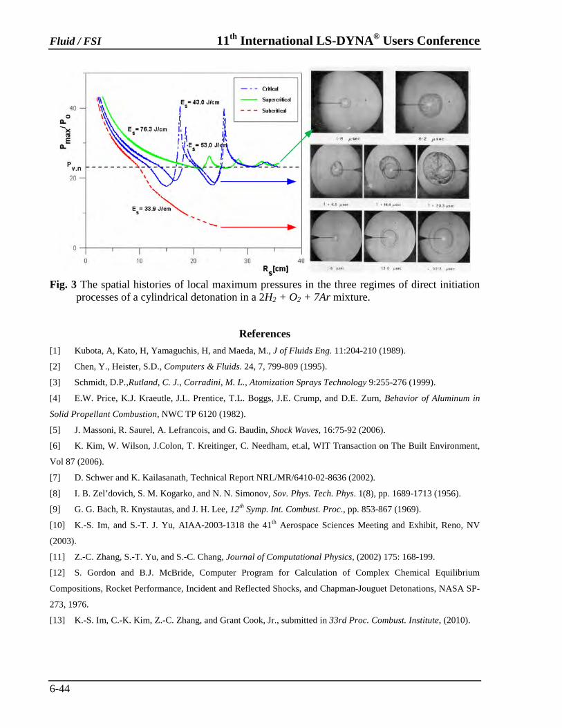
Figure 3 shows the simulation results of three regimes of direct initiation according to different initiation energy. The ratio of local maximum pressure to initial reactant pressure is plotted as a function of the radial locations of the leading shock wave. For reference, the pressure of the von-Neuman spike of the corresponding self sustained CJ detonation (for the driven section) is also plotted by dot line. In a series of calculations by incrementally increasing the values of the deposited initiation energy, the three regimes can be clearly observed. When the initial energy Es = 33.0 J/cm, the strong blast wave decays to a wave with peak pressures much lower than the CJ value, indicating a failed detonation initiation process. Two initial energies of Es = 43.0 J/cm and Es = 53.0 J/cm are in the critical regime. Distinct pressure peaks are observed. The deposited initiation energies are not high enough to sustain stable detonation waves. This unstable period ends at R = 30cm, and the waves become the self–sustained CJ detonation waves. With higher initiation energy for Es = 76.3 J/cm, the initial blast wave directly initiate the detonation wave, which expands and decays to the CJ value with mild instabilities. The corresponding experimental schlieren images are also illustrated in the figure.


6-44

Fig. 3 The spatial histories of local maximum pressures in the three regimes of direct initiation

processes of a cylindrical detonation in a 2H2 + O2 + 7Ar mixture.

References

[1] Kubota, A, Kato, H, Yamaguchis, H, and Maeda, M., J of Fluids Eng. 11:204-210 (1989).

[2] Chen, Y., Heister, S.D., Computers & Fluids. 24, 7, 799-809 (1995).

[3] Schmidt, D.P.,Rutland, C. J., Corradini, M. L., Atomization Sprays Technology 9:255-276 (1999).

[4] E.W. Price, K.J. Kraeutle, J.L. Prentice, T.L. Boggs, J.E. Crump, and D.E. Zurn, Behavior of Aluminum in

Solid Propellant Combustion, NWC TP 6120 (1982).

[5] J. Massoni, R. Saurel, A. Lefrancois, and G. Baudin, Shock Waves, 16:75-92 (2006).

[6] K. Kim, W. Wilson, J.Colon, T. Kreitinger, C. Needham, et.al, WIT Transaction on The Built Environment,

Vol 87 (2006).

[7] D. Schwer and K. Kailasanath, Technical Report NRL/MR/6410-02-8636 (2002).

[8] I. B. Zel’dovich, S. M. Kogarko, and N. N. Simonov, Sov. Phys. Tech. Phys. 1(8), pp. 1689-1713 (1956).

[9] G. G. Bach, R. Knystautas, and J. H. Lee, 12th Symp. Int. Combust. Proc., pp. 853-867 (1969).

[10] K.-S. Im, and S.-T. J. Yu, AIAA-2003-1318 the 41th Aerospace Sciences Meeting and Exhibit, Reno, NV

(2003).

[11] Z.-C. Zhang, S.-T. Yu, and S.-C. Chang, Journal of Computational Physics, (2002) 175: 168-199.

[12] S. Gordon and B.J. McBride, Computer Program for Calculation of Complex Chemical Equilibrium

Compositions, Rocket Performance, Incident and Reflected Shocks, and Chapman-Jouguet Detonations, NASA SP-

273, 1976.

[13] K.-S. Im, C.-K. Kim, Z.-C. Zhang, and Grant Cook, Jr., submitted in 33rd Proc. Combust. Institute, (2010).

Documents

FEA Information Engineering Journal - April 2012.pdf - feaiej