Embed Size (px)
Citation preview
Nutrition Assistance Program Report SeriesOffice of Research and Analysis
Family Nutrition Programs Report No. FSP-08-SAE
Feasibility of Assessing Causes of StateVariation in Food Stamp Program
Administrative Costs:
Final Report
United States Food andDepartment of NutritionAgriculture Service
September 2008
Non-Discrimination Policy
The U.S. Department of Agriculture (USDA) prohibits discrimination in all its programs and activitieson the basis of race, color, national origin, age, disability, and where applicable, sex, marital status,familial status, parental status, religion, sexual orientation, genetic information, political beliefs,reprisal, or because all or part of a person’s income is derived from any public assistance program. (Notall prohibited bases apply to all programs.)
Persons with disabilities who require alternative means for communication of program information(Braille, large print, audiotape, etc.) should contact USDA’s TARGET Center at (202) 720-2600 (voiceand TDD).
To file a complaint of discrimination, write to USDA, Director, Office of Civil Rights, 1400Independence Avenue, S.W., Washington, DC 20250-9410, or call (800) 795-3272 (voice) or(202) 720-6382 (TDD). USDA is an equal opportunity provider and employer.
Feasibility of Assessing Causes of StateVariation in Food Stamp Program
Administrative Costs:
Final Report
Authors:Christopher LoganJacob Alex Klerman
Submitted by: Submitted to:
Abt Associates, Inc. Office of Research and Analysis55 Wheeler Street Food and Nutrition ServiceCambridge, MA 02138 3101 Park Center Drive
Alexandria, VA 22302-1500
Project Director: Project Officer:Christopher Logan Jenny Laster Genser
This study was conducted under Contract number AG3198-D-07-0088 with the Food and NutritionService.
This report is available on the Food and Nutrition Service website: http://www.fns.usda.gov
Suggested Citation:U.S. Department of Agriculture, Food and Nutrition Service, Office of Research and Analysis, Feasibilityof Assessing Causes of State Variation in Food Stamp Program Administrative Costs: Final Report, byChristopher Logan and Jacob Alex Klerman. Project Officer: Jenny Laster Genser, Alexandria, VA:September 2008.
United States Food andDepartment of NutritionAgriculture Service
September 2008Family Nutrition Programs
Report No. FSP-08-SAE

Acknowledgments
The authors wish to thank Nancy Burstein, recently retired from Abt Associates Inc., for herthoughtful advice as internal Project Quality Advisor, and the production staff of Eileen Fahey,Katheleen Linton, and Jan Nicholson. Jenny Genser delivered essential support and helpfulcomments and advice as the Contracting Officer’s Representative. The following Food and NutritionService (FNS) staff provided helpful information for the report and commented on the document:from the Office of Research and Analysis, Kristen Hyatt, Hoke Wilson, and Carol Olander; from theFood Stamp Programs staff, John Bedwell; and from the Financial Management staff, Charles Okal.We also thank Kenneth Hanson of the Economic Research Service for his advice and feedback.
This report relies substantially on expert views from numerous officials who shared their time andinsights. First, we wish to thank the Food Stamp Program and Financial Management staffs of theMid-Atlantic, Mountain-Plains, Southeast, and Southwest FNS Regional Offices. We also wish tothank the Administration for Children and Families and the Division of Cost Allocation in the U.S.Department of Health and Human Services. Finally, we wish to thank the representatives of the fourStates that participated in in-depth interviews: Nevada, New Mexico, North Carolina, andPennsylvania. This report would not have been possible without the generous cooperation of theseofficials.
This study was sponsored by the Office of Research and Analysis, Food and Nutrition Service, U.S.Department of Agriculture as part of its ongoing research agenda. Points of view or opinions stated inthis report are those of the authors and do not necessarily represent the official position of the Food andNutrition Service.

Abt Associates Inc. Contents
Contents
Executive Summary .............................................................................................................................. iBackground ..................................................................................................................................iiData Sources ...............................................................................................................................iiiConceptual Framework...............................................................................................................iiiDetailed Cost Data Desirable to Explain Variation ....................................................................viExplanatory Variables................................................................................................................. ixFeasibility of Explaining Variation in SAE ................................................................................. xA Suggested Program of Research on Variation in SAE..........................................................xiv
Study 1: Exploratory Analysis of Existing Aggregate Cost Data................................... xvStudy 2: Survey-Based Decomposition of Certification Costs....................................... xvStudy 3: Exploratory Study of Automated Data Processing Costs...............................xviiStudy 4: Pilot Study of Approaches to Collecting Disaggregated Eligibility
Worker Time per Case.................................................................................................xviiStudy 5: In-Depth Collection of Accounting Data and Expert Interviews in
All States ....................................................................................................................xviiiStudy 6: Full-Scale Study Using Enhanced Eligibility Worker Time-Use Data ..........xviiiStudy 7: Full-Scale Study Merging Case Records with Eligibility Worker
Time-Use Data............................................................................................................xviiiStudy 8: Full-Scale Study Collecting Data on Average Time per Task by
Case Type .....................................................................................................................xix
PART I: INTRODUCTION AND CONCEPTUAL FRAMEWORK ............................................................... 1
Chapter 1: Introduction...................................................................................................................... 1Food Stamp Program Costs.......................................................................................................... 1Federal and State Perspectives on Variation in Administrative Expenses................................... 3Purpose and Research Questions ................................................................................................. 4
Feasibility of Obtaining Suitable Data for Analysis of Variation in SAE......................... 4Feasibility of Non-Experimental Methods for Explaining Variation in SAE.................... 5
Key Themes of This Report ......................................................................................................... 8Data Sources for This Report....................................................................................................... 9Organization of this Report........................................................................................................ 11
Chapter 2: Perspectives for Comparing State Administrative Expenditures for the FSP ......... 13Decomposing FSP SAE ............................................................................................................. 13
Accounting Decomposition ............................................................................................. 13Case Decomposition........................................................................................................ 15Task Decomposition........................................................................................................ 17
Determinants of FSP SAE.......................................................................................................... 20Implications of the Model .......................................................................................................... 23
Decomposing Observed Variation................................................................................... 23Understanding the Role of Specific Factors .................................................................... 24
Chapter 3: Possible Analysis Strategies .......................................................................................... 27How Would We Proceed with Ideal Cost Data?........................................................................ 27Reduced Form Models of Aggregate Data................................................................................. 29Alternative Disaggregated Models............................................................................................. 31
Contents Abt Associates Inc.
Simplified Models to Decompose Aggregate Cost ......................................................... 31Separate Models of Costs by Case Type......................................................................... 33An Index Approach to Caseload Heterogeneity.............................................................. 33A Simplified Model Focused on Task Frequency by Case Type.................................... 36More General Models ..................................................................................................... 39
Causation ................................................................................................................................... 39Fixed Effects ................................................................................................................... 41
Summary.................................................................................................................................... 42
Chapter 4: Potential Study Designs................................................................................................. 43Option 1: Modeling Available State-Level Data ...................................................................... 43
Statistical Methods.......................................................................................................... 44Aggregate State-Level SAE Data.................................................................................... 44Explanatory Variables..................................................................................................... 45
Overview of Additional Data Requirements for Other Approaches ......................................... 45Option 2: Analysis of Overhead and Eligibility Worker Time per Case.................................. 49Option 3: Analysis of Cost by Case Type ................................................................................ 50Option 4: Analysis of Overhead, Difficulty, and Intensity by Case Type................................ 51Option 5: Analysis of Time per Task, Task Frequency, Overhead, and Pay............................ 53
Ideal Approaches............................................................................................................. 53Simplified Approaches.................................................................................................... 55Potential Estimation Approaches .................................................................................... 57
PART II: ASSESSMENT OF DATA SOURCES FOR POTENTIAL STUDY DESIGNS............................... 59
Chapter 5: Comparability of Aggregate Reported State Administrative Expenses ................... 59Potential Errors Arising in the Allocation and Reporting of SAE............................................. 59Definition and Comparability of Reported Expenses for FSP Functions.................................. 61
Functions of Interest for Analyzing Variation in SAE.................................................... 61FSP Cost Reporting Categories of Interest ..................................................................... 62
Possible Biases and Random Errors in Allocation of SAE ....................................................... 65Local Agency Costs ........................................................................................................ 66Administrative Costs for Other Client Services.............................................................. 68Reporting of ADP Development and Operations Costs.................................................. 69State-Level Administrative Costs ................................................................................... 69
Comparability of Reported SAE Over Time ............................................................................. 70Changes in Allocation of Administrative Expenses........................................................ 70Consistency in the Timing of Reported Expenses .......................................................... 72
Summary.................................................................................................................................... 73
Chapter 6: Data on Eligibility Worker Time, Compensation, and Costs .................................... 75Data for Option 2....................................................................................................................... 77
Data Sources ................................................................................................................... 77Bias and Precision........................................................................................................... 80Data Formats and Retention Periods............................................................................... 80Data Collection Process .................................................................................................. 81Definition of Eligibility Worker...................................................................................... 81Call Centers and Case Processing Centers...................................................................... 84
Abt Associates Inc. Contents
Personnel Data on Worker Characteristics to Analyze Variation in Pay and Benefits ... 84Data for Option 3 ....................................................................................................................... 85
Defining Case Types for Analysis................................................................................... 86Existing Eligibility Worker Time Data............................................................................ 88Combining Existing Eligibility Worker Time Data and Case Records ........................... 89New Data Collection on Eligibility Worker Time by Case Type.................................... 90
Data for Option 4 ....................................................................................................................... 91Sample Sizes.................................................................................................................... 93
Data for Option 5 ....................................................................................................................... 95Data for Time per Task Estimates ................................................................................... 96Task Frequency Data ....................................................................................................... 98FSP Share of Eligibility Worker Costs.......................................................................... 100
Summary .................................................................................................................................. 100
Chapter 7: Decomposition of Reported Expenditures Other than Eligibility Worker Costs... 103Defining the Overhead Rate..................................................................................................... 104Concepts for Decomposing the Overhead Rate for Analysis................................................... 104
Labor versus Nonlabor .................................................................................................. 104Local versus State.......................................................................................................... 105Types of Nonlabor Costs ............................................................................................... 105State-Level Functions .................................................................................................... 105
Data for Decomposing Overhead Costs................................................................................... 105Cost Allocation Plans .................................................................................................... 105Accounting System Data ............................................................................................... 106Data on Non-Eligibility Worker Time and Pay............................................................. 108Methods for Obtaining Data for Decomposition of Overhead ...................................... 110
Data for Analysis of Data Processing Costs ............................................................................ 110
Chapter 8: Explanatory Variables................................................................................................. 113Overview of Explanatory Variables......................................................................................... 113Case Counts, Activity, and Performance Data......................................................................... 115
State Client Information Systems .................................................................................. 116Quality Control Sample Public Use Microdata ............................................................. 116Summary Reports .......................................................................................................... 117
Input Price Data ....................................................................................................................... 119National Surveys of Public Welfare Worker Pay .......................................................... 119Comparable Pay for Private Sector Workers................................................................. 120General Price or Cost of Living Indexes ....................................................................... 121Price Indexes for Inputs Other than Labor .................................................................... 121
General Environment ............................................................................................................... 122Economic Conditions .................................................................................................... 123State Fiscal Conditions .................................................................................................. 123Political Conditions ....................................................................................................... 124Social Conditions........................................................................................................... 124
Characteristics of State FSP Operations .................................................................................. 125FSP Policy Variables Databases.................................................................................... 125Welfare Rules Database................................................................................................. 125Surveys of State FSP Operations................................................................................... 126
Summary .................................................................................................................................. 127
Contents Abt Associates Inc.
PART III: CONCLUSIONS AND RECOMMENDATIONS ..................................................................... 129
Chapter 9: Conclusions and Recommendations .......................................................................... 129Feasibility of Obtaining Consistent Measures of SAE............................................................ 129Detailed Cost Data Desirable to Explain Variation................................................................. 130
Conceptual Framework for Defining Data Needs......................................................... 130Feasibility of Obtaining Data for Options 2, 3, 4 and 5 ................................................ 133Time Series of Cost Data Available.............................................................................. 135
Explanatory Variables ............................................................................................................. 137Feasibility of Explaining Variation in SAE............................................................................. 138A Suggested Program of Research on Variation in SAE ........................................................ 143
Study 1: Exploratory Analysis of Existing Aggregate Cost Data ................................ 143Study 2: Survey-Based Decomposition of Certification Costs .................................... 146Study 3: Exploratory Study of Automated Data Processing Costs .............................. 147Study 4: Pilot Study of Approaches to Collecting Disaggregated Eligibility
Worker Time per Case ................................................................................................ 147Study 5: In-Depth Collection of Accounting Data and Expert Interviews in
All States ..................................................................................................................... 148Study 6: Full-Scale Study Using Enhanced Eligibility Worker Time-Use Data .......... 148Study 7: Full-Scale Study Merging Case Records with Eligibility Worker
Time-Use Data ............................................................................................................ 149Study 8: Full-Scale Study Collecting Data on Average Time per Task by
Case Type.................................................................................................................... 149
Appendix A: Background on Food Stamp Program Administration ........................................ A-1FSP Administrative Functions................................................................................................. A-1
Certification .................................................................................................................. A-1Issuance of Benefits ...................................................................................................... A-1Employment and Training............................................................................................. A-2Nutrition Education....................................................................................................... A-2Automated Data Processing System Development and Operations.............................. A-2Fraud Control and Fair Hearings................................................................................... A-3Other State and Local Program Administration............................................................ A-3Composition of Total SAE............................................................................................ A-3
FSP Administrative Roles of Local Offices, State Agencies, and Other Organizations ......... A-3Local Offices................................................................................................................. A-4State Food Stamp Agency and Other Organizations..................................................... A-5
Appendix B: Accountability and Reporting of State FSP Administrative Expenditures......... B-1Allowable Expenditures ...........................................................................................................B-2Accounting Systems and Controls............................................................................................B-2Methods for Allocating Expenses to the FSP...........................................................................B-3Local Office Costs ....................................................................................................................B-4
Local Labor Costs ..........................................................................................................B-5Local Nonlabor Costs.....................................................................................................B-6
Abt Associates Inc. Contents
State Costs................................................................................................................................ B-7Data Processing and Telecommunications .................................................................... B-7Client Services............................................................................................................... B-7Policy, Program Oversight, and Statewide Administration........................................... B-8
Reporting of Food Stamp Administrative Expenses to FNS.................................................... B-8
References .........................................................................................................................................R-1
Contents Abt Associates Inc.
List of Exhibits
Exhibit ES.1: Research Options, Data Requirements, and Potential Data Sources ............................ vii
Exhibit ES.2: Comparison of Feasibility, Advantages, and Limitations of Research Options ............ xi
Exhibit ES.3: Suggested Program of Studies of Interstate Variation in FSP StateAdministrative Expenses .................................................................................................................. xvi
Exhibit 1.1: Characteristics of State Agencies Participating in Study Interviews .............................. 10
Exhibit 2.1: Determinants of Components of Variation in SAE......................................................... 21
Exhibit 4.1: Explanatory Data Elements for Models of State Administrative Expensesfor the FSP ......................................................................................................................................... 46
Exhibit 4.2: Research Options, Data Requirements, and Potential Data Sources............................... 48
Exhibit 8.1: Explanatory Data Elements for Models of State Administrative Expenses forthe FSP............................................................................................................................................. 114
Exhibit 9.1: Research Options, Data Requirements, and Potential Data Sources............................. 132
Exhibit 9.2: Feasible Time Periods for Cost Data Required by Research Options........................... 136
Exhibit 9.3: Comparison of Feasibility, Advantages, and Limitations of Research Options............ 139
Exhibit 9.4: Suggested Program of Studies of Interstate Variation in FSP StateAdministrative Expenses ................................................................................................................. 144
Abt Associates Inc. Executive Summary i
Executive Summary
In September 2007, the Food and Nutrition Service (FNS), U.S. Department of Agriculture (USDA)awarded to Abt Associates Inc. the Feasibility of Assessing Causes of State Variation in Food StampProgram (FSP) Administrative Costs Study (hereafter the Feasibility Study).1 The purpose of thestudy is to develop a menu of approaches for better understanding how and why State administrativeexpenses (SAE) vary between States.
The Feasibility Study addresses two sets of research questions: issues of the data sources to be used,and alternatives for analyzing and explaining variations in administrative expenses. In particular,
Is it possible to measure food stamp administrative expenses consistently enough acrossStates to credibly assess the degree of variation? If it is possible, what are the alternativeways to measure such expenses? Are new data required? If so, what level of effort would berequired and what challenges would need to be addressed to obtain such data?
Can the causes of variation in State food stamp administrative costs be explained in theabsence of experimental design? Why or why not? If so, what are the alternativeapproaches, and what are the advantages and disadvantages of each? Which approach isrecommended and why?
These questions are interrelated. The types of data required depend on the methods to be used, andthe feasible methods depend on the feasible data sources.
In this report, we find that State administrative expenses for the FSP can be compared across States,with some limitations, and we present several feasible approaches for explaining the causes ofvariation in SAE, albeit with varying degrees of confidence. We first present a conceptual frameworkfor the possible causes of variation in SAE and a series of general, nonexperimental analyticapproaches based on this framework. The conceptual framework describes how SAE may be affectedby State characteristics including population demographics, economic conditions, politicalpreferences, policies, and management strategies. We describe ideal data and then explain why theywould not be feasible to obtain. We then present and compare five feasible options for making thesecomparisons and analyzing the sources of variation in SAE. These options would use varyingcombinations of existing national databases, State accounting records, and new data collection. Theoptions focus on certification costs in general, and specifically on the costs of eligibility workers, i.e.,personnel who make eligibility determinations.
There are clear trade-offs among the options. Use of existing national databases would require strongassumptions and limit the number of explanatory variables. Collecting accounting records wouldallow more realistic assumptions and use of disaggregated data to increase the ability to explainvariation, at a relatively low cost and burden on the States. New data collection would support moredisaggregated, robust, and definitive analysis, but would entail moderate to high costs and burden,depending on the approach and the scope. Thus, FNS has a range of choices for understanding
1 On October 1, 2008, the Food Stamp Program will change its name to the Supplemental NutritionAssistance Program (SNAP).
ii Executive Summary Abt Associates Inc.
variation in SAE among the States. We facilitate these choices by presenting a recommendedsequence of studies using the most feasible and promising options.
In this executive summary, we begin with the purpose and background of the study. We thensummarize the key concepts for analyzing variation in SAE. Next, we discuss the issues of thecomparability and availability of cost data. We then present the five options and summarize theirrelative strengths and weaknesses. We conclude with an overview of the recommended sequence ofstudies.
Background
The FSP provides assistance to low-income households so that they can purchase an adequate supplyof nutritious food. The FSP is the largest of the 15 domestic food and nutrition assistance programsadministered by the US Department of Agriculture’s Food and Nutrition Service (FNS). The FSPserved 26.5 million people in an average month in Fiscal Year 2007, for a total Federal cost of $33.2billion, of which $30.4 billion were for food stamp benefits (FNS, 2008a).
The FSP is jointly administered by the Federal government and the States.2 The Federal governmentsets the basic program parameters and pays for all benefits. State governments choose programoptions from among those allowed by Federal statute and FNS regulations, and operate the program.
Expenditures for State and local administration of the FSP are considerable and vary substantiallyacross States and over time. In FY2007, SAE totaled $5.5 billion, representing 17 percent of totalFSP expenditures (FNS, 2008a). This is equivalent to $469 per participating household.3 The rangein FY2007 was from $169 in South Carolina to $1,169 in California, more than a nearly seven-folddifference. Between 1989 and 2005, the average administrative expenditure for the nation (in 2005dollars) ranged from $346 and $657 per household (Logan, Kling and Rhodes, 2008).
Administrative costs represent a greater share of total program costs in the FSP than in several otherhuman service programs, including the Temporary Assistance for Needy Families (TANF) andUnemployment Insurance (UI) programs, but less than in others, such as adoption assistance andfoster care, according to a recent General Accountability Office study (GAO, 2006). The FSP alsospends a greater percentage of funds on administrative costs than the Earned Income Tax Creditprogram (Isaacs, 2008). While there are important differences between these programs and in theirdefinitions of administrative costs, such comparisons highlight the need to understand what drives thedifferences between low-cost and high-cost States, and whether there are lessons for improving theefficiency of the FSP.
2 For the purposes of this report, references to “States” include the 50 States and the District of Columbia butexclude Guam and the Virgin Islands, which are not expected to be part of a cost study because of theirunique circumstances. Puerto Rico is also excluded because it receives a block grant in lieu of operatingthe FSP. “FY” refers to the Federal fiscal year, October 1 through September 30.
3 This estimate is computed as the ratio of total SAE to average monthly food stamp households. The actualnumber of unique households participating in the FSP during a year is more than the average of themonthly counts, but the annual unique count is not regularly reported. The annual cost per FSP householdas defined above is equal to 12 times the average monthly cost per FSP household, and thus the annual andmonthly cost per household are perfectly correlated.
Abt Associates Inc. Executive Summary iii
Data Sources
For this study, we reviewed a range of published reports on administrative costs in the FSP andsimilar programs, as documented in the references of both memoranda. We identified relevantpublications through key agencies’ web sites (FNS, USDA Office of Inspector General, GovernmentAccountability Office, and Department of Health and Human Services) and through our priorresearch experience. We also conducted semi-structured interviews with Federal officials (includingFNS Headquarters, four regional FNS offices, and the Department of Health and Human Services)and with program and finance officials of four States: Nevada, New Mexico, North Carolina, andPennsylvania. These interviews gathered data on possible problems with comparing SAE, possibleextant data for analysis of SAE at the State and local levels, and opinions on the reasons for thevariation in SAE.
In the report, we make generalizations based on these data sources. All generalizations are subjectto the caution that they are based on the limited data sources for the study. In addition, wherewe found conflicting evidence or heard differing views on a topic, we note this as an area ofuncertainty. The discussion of issues for future research reflects the limitations of our informationand the important areas of uncertainty. In particular, we identify information that should be collectedto resolve uncertainties before undertaking some approaches or analyses.
Conceptual Framework
We divide the factors that may contribute to variation in SAE between uncontrollables andcontrollables. Uncontrollables are economic, demographic, and political conditions which are out ofthe control of the States. Controllables are policy and management choices made by State or localofficials. A key goal of any study of FSP SAE should be to establish the relative importance ofuncontrollables and controllables. If variation in SAE is mainly due to uncontrollables, there is lessscope for cost savings than if variation in SAE is mainly due to controllables that the Federalgovernment could influence through policies or financial incentives. Efforts to reduce SAE wouldneed to take into account the possible effects on FSP payment accuracy, timeliness of applicationprocessing, and access.
In addition, Federal and State officials may be interested in the effects of specific policy andmanagement choices. Does adopting semi-annual reporting cut SAE? By how much? Are county-administered systems more expensive? By how much? Do investments in computer technology leadto long term savings in total SAE?
This report considers strategies for explaining overall interstate variation in FSP SAE (and the extentto which it is due to uncontrollables and controllables), and for estimating the cost implications ofspecific policy and management choices. The approach to these questions must be non-experimental,because States have substantial autonomy in administering the FSP.
The key challenges for non-experimental studies of SAE for the FSP are (1) known and unknownuncontrollables that are directly related to SAE and to policy or management choices that may affectSAE, and (2) separating the effects of large numbers of specific uncontrollables and controllables thatmay contribute to variation in SAE. The key strategies for dealing with these challenges are (1)
iv Executive Summary Abt Associates Inc.
disaggregating SAE into components with smaller and better-specified sets of potential explanatoryfactors, and (2) analyzing changes in explanatory variables and SAE within States over time (i.e.,differences in differences) to control for unknown characteristics of States that may affect both SAEand the controllables of interest.
We define three conceptual levels for decomposing SAE for the FSP: the accounting, case, and tasklevels. At the accounting level, the total SAE for a period of time in a State is the sum ofexpenditures for all inputs purchased (labor, computer time, office space, etc.). For each input, thetotal expenditure is the product of the quantity, the average price, and the average share allocated tothe FSP. Inputs can be shared across programs with respect to cases (eligibility worker time for anapplication for food stamps and other benefits), with respect to workers (general training for multipleprograms), and with respect to higher levels in the agency. Cost allocation rules and the mix ofprograms sharing cases with the FSP determine the FSP share of expenditures. This framework leadsto a decomposition of variation in input quantities, prices, and the FSP share, and also to analysis ofthe relative importance of different inputs. This is important because input costs are nearlyuncontrollable. States located in regions with high wages and rents are likely to have higher SAE.
At the case level, the total SAE is the sum of expenditures for all FSP cases. Cases differ incomposition (presence of children, elderly, other adults, or noncitizens), sources of income,participation in other programs, and other characteristics. Different types of cases will have differentaverage costs, because different quantities of inputs are used. The average cost for each type of caseis determined by the average quantity of each input, the average prices of those inputs, and the shareof those input costs allocated to the FSP. More inputs for a given type of case may contribute to abetter level of performance, where dimensions of performance include payment accuracy, timeliness,and accessibility for eligible households. Taking the averages for case types and weighting by theirshare of the FSP caseload gives the overall average cost per FSP case. In this framework, variation inSAE can in principle be decomposed into variation in input prices, input quantities per case by typeof case, FSP share of costs by case type, and case mix (percentage by type). This is importantbecause case mix is largely uncontrollable, although State policies may have minor effects. SomeStates have more cases with earnings or more noncitizens. In as much as these types of cases requiremore case management, SAE will be higher in States with more of these cases.
At the task level, the total SAE is the sum of expenditures on all administrative tasks for all FSPcases. Thus, SAE varies because of differences in what States do (task frequency) and what inputsthey use to do these tasks. Both task frequency and the quantity of inputs may affect the level ofperformance. The average cost of a task is determined by the input quantities, input prices, and theFSP share of the cost. The input quantity includes what is actually used to perform the specific taskand a share of the quantity used for more general FSP administration that is not task-specific (e.g., thesalary of the State FSP director). Input quantities, FSP shares, and task frequency vary by type ofcase; these factors jointly determine the average cost per case for each type of case. The case mix andthe average cost per case by type determine the overall average cost per case.
Thus, at the task level, variation in SAE can in principle be decomposed into variation in inputprices, input quantities per task by task and type of case, FSP share of costs by task and case type,frequency of tasks by case type, and case mix (percentage by type). The ideal data for thisdecomposition at the task level do not exist and are not likely to exist, but we use thisframework to develop more feasible approaches. This final decomposition is important because,presumably part of the reason why some States have higher SAE is that they do different tasks.
Abt Associates Inc. Executive Summary v
Ideally, we would like to know if some State’s SAE was higher because it was doing more outreach,giving more help to clients in completing applications, processing applications faster, processingcases with fewer errors, or asking applicants to wait less time before seeing an eligibility worker. Ifwe understood the extent to which SAE in different States varies because they are doing differenttasks, the Federal government could consider State rules or financial incentives to alter Statedecisions about which tasks to do and how often to do them.
In this report, we present a conceptual model of the factors that determine the components ofvariation in the task level framework (caseload size and mix, input prices, FSP share of costs, tasksperformed, and inputs per task). The principal hypotheses are summarized below.
Market prices of inputs, caseload size, and case mix are “uncontrollables” primarilydetermined by the State’s population and economy. State policies have a minor effect on theFSP caseload and case mix.
The FSP share of costs is affected by both State policies and the socioeconomiccharacteristics of the State population. Policies determine the share of costs for a taskinvolving a given combination of programs, while the population determines the proportionof FSP cases participating in other programs.
Tasks performed for each case type are determined by State policies, the State budget for FSPSAE, and management strategies.
Inputs per task for each case type are determined by the State budget and managementstrategies.
The accounting, case, and task levels interact. A task-saving policy change will not directly affectFSP SAE unless the staffing level (total input of eligibility workers) is cut at the same time. Thus, atleast in the short run, what we observe is not the full potential savings of the change, but the savingsrealized by the agency when it implements the change. Ideally, the State would adjust staffing levelsin response to opportunities for savings and demand for increased staffing. In reality, staffingadjustments are difficult to make in the short run—both when there are potential savings and whenthe caseload rises more than was anticipated when the State FSP budget was set. With theseconstraints, it seems likely that there are differences in the frequency of tasks performed and thequality of performance, in terms of accuracy, timeliness, and making the FSP accessible to eligiblehouseholds.
While the ideal task-level decomposition is not possible, the options developed in this report specifyfeasible approaches to decompose the overall variation in SAE into the contributions of case mix,input prices, tasks performed, input per task, and FSP share of costs. They also provide strategies forunderstanding the role of specific factors, both uncontrollables and controllables. One generalstrategy is the “reduced form” approach, regressing total SAE on the factors of interest. The otherstrategy is a “structural” approach that simplifies but approximate the conceptual model in a systemof equations, using proxies that are obtainable for the detailed information that is not.
vi Executive Summary Abt Associates Inc.
Detailed Cost Data Desirable to Explain Variation
It is highly desirable to disaggregate SAE as much as practical along the dimensions of the ideal tasklevel framework. While a conventional regression analysis of aggregate SAE at the State level couldcertainly be undertaken, and indeed is one of the recommended approaches, it would have twoimportant limitations. First, with a large number of possible explanatory factors and only 51 States(counting the District of Columbia), we are likely to run out of degrees of freedom to estimate effectswith confidence. Second, a linear specification with variables having additive effects appears to be apoor approximation to the true model.
To disaggregate SAE along the lines of the conceptual framework, we would need some or all of thefollowing kinds of cost data, in addition to aggregate SAE per case by State and year:
breakdown of SAE among inputs, particularly between eligibility workers and other inputs prices and quantities of inputs, particularly eligibility worker time and pay distribution of eligibility worker time by type of case frequency of eligibility worker tasks and time per task.
We focus on eligibility worker labor as the input of greatest interest because these workers play thelargest role in the usual certification process.
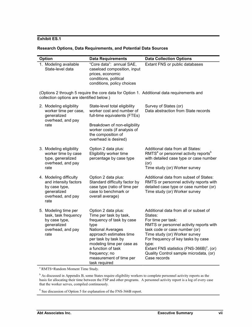
The specific data requirements and the feasibility of meeting those requirements depend on theapproach to disaggregating SAE. We have identified five feasible options for explaining the variationin SAE using extant or new cost data at varying levels of aggregation. The five options and their datarequirements are summarized in Exhibit ES.1. One option (Option 1) would model aggregate State-level SAE per case (specifically, certification costs) as reported by States to FNS. These cost data arecertainly available.
The other four options would implement different parts of the ideal disaggregation of SAE. Option 2would break down total certification costs into three key variables: eligibility worker hours,eligibility worker pay per hour, and the “generalized overhead rate”, defined as the ratio of all othercosts to eligibility worker costs. This option would require data from State financial records.
Options 3 and 4 would further break down the eligibility worker hours by case type; Option 3 woulddo this for all States, while Option 4 would do this in a sample of States and use the data to constructa difficulty index of the relative effort for each type of case. These options would thus require dataon the distribution of eligibility worker time by type of case.
For Option 3, methods are available that could collect the desired data on eligibility worker hours bycase type in all States. Such data do not appear to exist in most States, except for the percentagedistribution of eligibility worker time by program combination (FS-only, FS and Medicaid, etc.).This information exists in States that conduct that administer programs jointly and collect thisinformation for cost allocation purposes through random-moment time studies (RMTS) or activityreports. These existing data are feasible to collect and would be informative, but the combination ofprograms is only one of the case type dimensions of interest. We would also like information onrelative effort required for other case characteristics that are likely to shift SAE per case. Those case
Abt Associates Inc. Executive Summary vii
Exhibit ES.1
Research Options, Data Requirements, and Potential Data Sources
Option Data Requirements Data Collection Options1. Modeling available
State-level data“Core data”: annual SAE,caseload composition, inputprices, economicconditions, politicalconditions, policy choices
Extant FNS or public databases
(Options 2 through 5 require the core data for Option 1. Additional data requirements andcollection options are identified below.)
2. Modeling eligibilityworker time per case,generalizedoverhead, and payrate
State-level total eligibilityworker cost and number offull-time equivalents (FTEs)
Breakdown of non-eligibilityworker costs (if analysis ofthe composition ofoverhead is desired)
Survey of States (or)Data abstraction from State records
3. Modeling eligibilityworker time by casetype, generalizedoverhead, and payrate
Option 2 data plus:Eligibility worker timepercentage by case type
Additional data from all States:RMTSa or personnel activity reportsb
with detailed case type or case number(or)Time study (or) Worker survey
4. Modeling difficultyand intensity factorsby case type,generalizedoverhead, and payrate
Option 2 data plus:Standard difficulty factor bycase type (ratio of time percase to benchmark oroverall average)
Additional data from subset of States:RMTS or personnel activity reports withdetailed case type or case number (or)Time study (or) Worker survey
5. Modeling time pertask, task frequencyby case type,generalizedoverhead, and payrate
Option 2 data plus:Time per task by task,frequency of task by casetypeNational Averagesapproach estimates timeper task by task bymodeling time per case asa function of taskfrequency; nomeasurement of time pertask required
Additional data from all or subset ofStates:For time per task:RMTS or personnel activity reports withtask code or case number (or)Time study (or) Worker surveyFor frequency of key tasks by casetype:Extant FNS statistics (FNS-366B)c, (or)Quality Control sample microdata, (or)Case records
a RMTS=Random Moment Time Study.b As discussed in Appendix B, some States require eligibility workers to complete personnel activity reports as thebasis for allocating their time between the FSP and other programs. A personnel activity report is a log of every casethat the worker serves, compiled continuously.c See discussion of Option 5 for explanation of the FNS-366B report.
viii Executive Summary Abt Associates Inc.
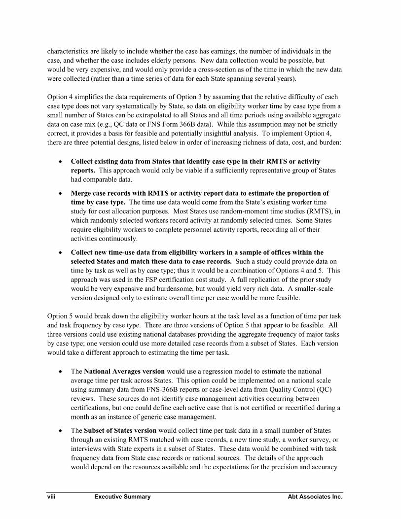
characteristics are likely to include whether the case has earnings, the number of individuals in thecase, and whether the case includes elderly persons. New data collection would be possible, butwould be very expensive, and would only provide a cross-section as of the time in which the new datawere collected (rather than a time series of data for each State spanning several years).
Option 4 simplifies the data requirements of Option 3 by assuming that the relative difficulty of eachcase type does not vary systematically by State, so data on eligibility worker time by case type from asmall number of States can be extrapolated to all States and all time periods using available aggregatedata on case mix (e.g., QC data or FNS Form 366B data). While this assumption may not be strictlycorrect, it provides a basis for feasible and potentially insightful analysis. To implement Option 4,there are three potential designs, listed below in order of increasing richness of data, cost, and burden:
Collect existing data from States that identify case type in their RMTS or activityreports. This approach would only be viable if a sufficiently representative group of Stateshad comparable data.
Merge case records with RMTS or activity report data to estimate the proportion oftime by case type. The time use data would come from the State’s existing worker timestudy for cost allocation purposes. Most States use random-moment time studies (RMTS), inwhich randomly selected workers record activity at randomly selected times. Some Statesrequire eligibility workers to complete personnel activity reports, recording all of theiractivities continuously.
Collect new time-use data from eligibility workers in a sample of offices within theselected States and match these data to case records. Such a study could provide data ontime by task as well as by case type; thus it would be a combination of Options 4 and 5. Thisapproach was used in the FSP certification cost study. A full replication of the prior studywould be very expensive and burdensome, but would yield very rich data. A smaller-scaleversion designed only to estimate overall time per case would be more feasible.
Option 5 would break down the eligibility worker hours at the task level as a function of time per taskand task frequency by case type. There are three versions of Option 5 that appear to be feasible. Allthree versions could use existing national databases providing the aggregate frequency of major tasksby case type; one version could use more detailed case records from a subset of States. Each versionwould take a different approach to estimating the time per task.
The National Averages version would use a regression model to estimate the nationalaverage time per task across States. This option could be implemented on a national scaleusing summary data from FNS-366B reports or case-level data from Quality Control (QC)reviews. These sources do not identify case management activities occurring betweencertifications, but one could define each active case that is not certified or recertified during amonth as an instance of generic case management.
The Subset of States version would collect time per task data in a small number of Statesthrough an existing RMTS matched with case records, a new time study, a worker survey, orinterviews with State experts in a subset of States. These data would be combined with taskfrequency data from State case records or national sources. The details of the approachwould depend on the resources available and the expectations for the precision and accuracy
Abt Associates Inc. Executive Summary ix
of the estimates. Analysis based on State case records would have to be mapped into taskcategories in national sources to generalize to all States.
The All States version would collect time per task in all States. While any of the methodsfor the Subset of States version might in principle be used in all States, only the expertinterview method appears practical, considering the costs and burden. Given the uncertaintyabout the validity of such data, it would be preferable to combine this version with one of theother versions of Option 5.
Under all of these options, additional State-level data would be needed to break down the overheadrate into components for separate analysis (labor vs. non-labor, local vs. State, etc.).
Explanatory Variables
The review of sources identified a wealth of data that can be used to analyze variation in SAE. Inparticular, there are strong national databases with State-level time series data on the following typesof explanatory variables:
case counts and characteristics frequency of certification and recertification, by case type pay for public welfare workers and comparable private sector occupations economic conditions State revenues and expenditures political and social conditions FSP and welfare rules.
There are, however, some important limitations and challenges.
For data on case mix other than the public assistance/non-public assistance breakdown inFNS data, analysts will likely need to process QC microdata or State client data. Analysisstrategies for QC data need to define case types so that none is too small a percentage of thecaseload, taking into account the QC sample size in each State and the effects of weighting onthe precision of estimates.
State client data must be processed to determine the frequency of activities other thancertification, recertification, and denied applications.
While wage rates are available at the State level, benchmarks for benefits are available onlyat the regional level, and union/non-union wage differentials are available only nationally andfor specific metropolitan areas.
There are no State-level benchmarks or indices for the costs of resources other than laborused in FSP State and local operations. It appears that the most practical strategy fornormalizing nonlabor costs is to use a general cost of living index as a proxy.
FSP procedures and operating characteristics are not documented on an ongoing basis,although some one-time surveys are available.
x Executive Summary Abt Associates Inc.
Feasibility of Explaining Variation in SAE
Any of the specified options would provide important insights in variation in SAE, well beyond theexisting literature. The options would, to varying degrees, permit analysis of how SAE varies withdifferences in case mix, wages and other input prices, task frequency, time per task, and FSP share ofcosts. The options that disaggregate SAE would allow analysis of the factors that drive each of thesecomponents of the overall variation in SAE. To the extent that analysis can identify theuncontrollable factors affecting SAE, the options would permit estimates of normalized SAE (takingout the effects of uncontrollables) that could then be modeled in relation to State performance,including payment accuracy, timeliness, and program accessibility.
There are important trade-offs among the options on five basic dimensions:
the degree of uncertainty about the technical feasibility of the option
the number of years that are technically and practically feasible to include in the analysis, andthus the feasibility of using difference-in-differences (DD) methods
the limitations of the analysis due to the underlying assumptions
the ability to estimate the effects of specific variables on SAE (controllables anduncontrollables)
the relative cost and burden of the potential research, based on the scope of the data collectionand the number and types of respondents.
In general, the options that are more practical (in terms of technical feasibility, cost, and burden onStates) are the ones that use more aggregated data, and therefore have less potential to explainvariation. The options that will disaggregate costs into more factors entail more cost and burden.Therefore, these options by themselves would be more likely to be limited to cross-sectional analysis,although they could be combined with the more aggregated time-series data for DD analysis. Inaddition, there are significant feasibility questions about some of these options.
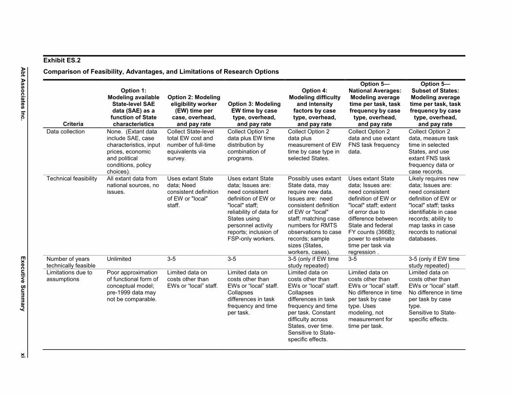
Exhibit ES.2 compares the research options on these dimensions, summarizing the feasibilityassessment for each option discussed in this report. We exclude versions of Option 3, 4, and 5 thatwe have discussed in the report but view as infeasible due to lack of requisite data, high likelihood oferrors in data, or high cost or burden. Readers may differ in their views of the feasible level of costand burden for studies of SAE. Preliminary research suggested in the next section could change theassessment of the options that are not identified among the feasible set.
Option 1, the modeling of existing aggregate State-level SAE data, is by far the most feasible option.There is no doubt about the technical feasibility, and it has the lowest cost and burden of the options.It is also the only option that by itself would support a robust DD time-series analysis with State fixedeffects. It could readily be combined with any of the other options as an initial exploratory stage or asa complement. On the other hand, Option 1 uses the most aggregated cost data. This is a veryimportant limiting factor on the ability to model the effects of FSP policies and management choices.Other limitations are the assumed functional form and the uncertain comparability between pre-1999
Ab
tA
ssociates
Inc.
Execu
tiveS
um
mary
xi
Exhibit ES.2
Comparison of Feasibility, Advantages, and Limitations of Research Options
Criteria
Option 1:Modeling available
State-level SAEdata (SAE) as a
function of Statecharacteristics
Option 2: Modelingeligibility worker
(EW) time percase, overhead,
and pay rate
Option 3: ModelingEW time by casetype, overhead,
and pay rate
Option 4:Modeling difficulty
and intensityfactors by casetype, overhead,
and pay rate
Option 5—National Averages:Modeling averagetime per task, taskfrequency by case
type, overhead,and pay rate
Option 5—Subset of States:Modeling averagetime per task, taskfrequency by case
type, overhead,and pay rate
Data collection None. (Extant datainclude SAE, casecharacteristics, inputprices, economicand politicalconditions, policychoices).
Collect State-leveltotal EW cost andnumber of full-timeequivalents viasurvey.
Collect Option 2data plus EW timedistribution bycombination ofprograms.
Collect Option 2data plusmeasurement of EWtime by case type inselected States.
Collect Option 2data and use extantFNS task frequencydata.
Collect Option 2data, measure tasktime in selectedStates, and useextant FNS taskfrequency data orcase records.
Technical feasibility All extant data fromnational sources, noissues.
Uses extant Statedata; Needconsistent definitionof EW or "local"staff.
Uses extant Statedata; Issues are:need consistentdefinition of EW or"local" staff;reliability of data forStates usingpersonnel activityreports; inclusion ofFSP-only workers.
Possibly uses extantState data, mayrequire new data.Issues are: needconsistent definitionof EW or "local"staff; matching casenumbers for RMTSobservations to caserecords; samplesizes (States,workers, cases).
Uses extant Statedata; Issues are:need consistentdefinition of EW or"local" staff; extentof error due todifference betweenState and federalFY counts (366B);power to estimatetime per task viaregression .
Likely requires newdata; Issues are:need consistentdefinition of EW or"local" staff; tasksidentifiable in caserecords; ability tomap tasks in caserecords to nationaldatabases.
Number of yearstechnically feasible
Unlimited 3-5 3-5 3-5 (only if EW timestudy repeated)
3-5 3-5 (only if EW timestudy repeated)
Limitations due toassumptions
Poor approximationof functional form ofconceptual model;pre-1999 data maynot be comparable.
Limited data oncosts other thanEWs or “local” staff.
Limited data oncosts other thanEWs or “local” staff.Collapsesdifferences in taskfrequency and timeper task.
Limited data oncosts other thanEWs or “local” staff.Collapsesdifferences in taskfrequency and timeper task. Constantdifficulty acrossStates, over time.Sensitive to State-specific effects.
Limited data oncosts other thanEWs or “local” staff.No difference in timeper task by casetype. Usesmodeling, notmeasurement fortime per task.
Limited data oncosts other thanEWs or “local” staff.No difference in timeper task by casetype.Sensitive to State-specific effects.
xiiE
xecutive
Su
mm
aryA
bt
Asso
ciatesIn
c.
Exhibit ES.2
Comparison of Feasibility, Advantages, and Limitations of Research Options (continued)
Criteria
Option 1:Modeling available
State-level SAEdata (SAE) as a
function of Statecharacteristics
Option 2: Modelingeligibility worker
(EW) time percase, overhead,
and pay rate
Option 3: ModelingEW time by casetype, overhead,
and pay rate
Option 4:Modeling difficulty
and intensityfactors by casetype, overhead,
and pay rate
Option 5—National Averages:Modeling averagetime per task, taskfrequency by case
type, overhead,and pay rate
Option 5—Subset of States:Modeling averagetime per task, taskfrequency by case
type, overhead,and pay rate
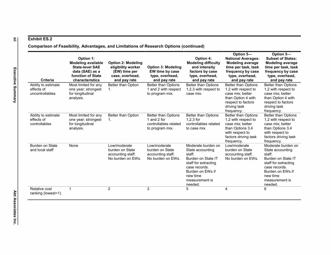
Ability to estimateeffects ofuncontrollables
Most limited for anyone year; strongestfor longitudinalanalysis.
Better than Option1.
Better than Options1 and 2 with respectto program mix.
Better than Options1,2,3 with respect tocase mix.
Better than Options1,2 with respect tocase mix; betterthan Option 4 withrespect to factorsdriving taskfrequency.
Better than Options1,2 with respect tocase mix; betterthan Option 4 withrespect to factorsdriving taskfrequency.
Ability to estimateeffects ofcontrollables
Most limited for anyone year; strongestfor longitudinalanalysis.
Better than Option1.
Better than Options1 and 2 forcontrollables relatedto program mix.
Better than Options1,2,3 forcontrollables relatedto case mix.
Better than Options1,2 with respect tocase mix; betterthan Options 3,4with respect tofactors driving taskfrequency.
Better than Options1,2 with respect tocase mix; betterthan Options 3,4with respect tofactors driving taskfrequency.
Burden on Stateand local staff
None Low/moderateburden on Stateaccounting staff.No burden on EWs.
Low/moderateburden on Stateaccounting staff.No burden on EWs.
Moderate burden onState accountingstaff.Burden on State ITstaff for extractingcase records.Burden on EWs ifnew timemeasurement isneeded.
Low/moderateburden on Stateaccounting staff.No burden on EWs.
Moderate burden onState accountingstaff.Burden on State ITstaff for extractingcase records.Burden on EWs ifnew timemeasurement isneeded.
Relative costranking (lowest=1)
1 2 3 5 4 6
Abt Associates Inc. Executive Summary xiii
data and later years. For explanatory variables that change substantially within States over time, theability to conduct longitudinal analysis using DD or other appropriate methods somewhat mitigatesthe limitation of aggregate data.
Option 2, Option 3, and Option 5-National Averages would use existing data from State accountingreports or spreadsheets and are therefore also likely to be feasible. (The feasible version of Option 3would collect existing data on eligibility worker time distribution by program combination.) Becauseof the use of existing aggregate accounting data in State records, these options rank second, third, andfourth (respectively) in expected cost. These options would have low to moderate burden on Stateaccounting personnel and no burden on eligibility workers. These options would substantiallyimprove the ability to identify major factors associated with variation in SAE. All three optionswould allow separate analysis of variation in eligibility worker time, pay, and overhead. Option 3would add further insight into the effects of cost-sharing among programs, while Option 5-NationalAverages would add insights into the factors driving task frequency and their impacts on SAE. Keylimitations for these three options, as well as the more costly options, would be: the challenge ofconsistently measuring eligibility worker time and costs, limited data on overhead, and thesimplification of all costs other than eligibility worker pay as overhead.
A limited version of Option 5-All States based on interviews with State experts is not listed in theexhibit but could be implemented at a low cost and no burden to eligibility workers. This optionwould collect expert estimates of eligibility worker time per task from every State. This approachwould provide estimates of national average time per task based on data from all States, instead ofrelying on regression analysis (as in Option 5-All States) or on a limited number of States (as inOption 5-Subset of States. While the individual State estimates could be used for exploratoryanalysis, there is real uncertainty about the level of accuracy for interview-based estimates and thevalidity of the methodology for State-level comparisons. Therefore, we view this option as apotential adjunct to other options, rather than a primary option on its own.
Option 4 and Option 5-Subset of States would provide the richest data (among the options that weconsider feasible) and, on balance, the best opportunities to identify the factors associated withvariation in SAE. Both options would generalize from data collected in a sample of States. Asindicated in Exhibit 9.3, Option 4 would collect eligibility worker time by case type in selected Statesto estimate standard difficulty factors for case types. Option 5-Subset of States would collecteligibility worker time per task in selected States to estimate the average time per task. These optionsare clearly strongest for estimating the variation associated with factors that do not changesubstantially within States over the time period that is feasible to study. The disaggregation of SAEwould allow more focused analysis of the variables that are relevant to each of the six components ofvariation (FSP share, case mix, overhead, eligibility worker pay, task frequency, and time per task;Option 4 collapses the last two components). This analysis does depend on the simplifyingassumptions of these options, but the alternative would be much more costly and burdensome studies.The practical downside of these options is that they require more data and thus would be more costlythan the other four options.4
4 While the options are numbered 1 through 5, there are two different versions of Option 5 among thoselisted in Exhibit 9.3.
xiv Executive Summary Abt Associates Inc.
While Option 4 and Option 5-Subset of States would complement each other, there may be a need tochoose between them. This choice is not clear, because of several unknown feasibility questions: theavailability of existing data that would facilitate these options, the feasibility of matching RMTS datawith case records, the tasks identifiable in case records, and the sample size requirements for specificdata collection approaches. Analysis conducted via Option 1 might point to Option 4 or Option 5 asthe more likely to explain variation in SAE.
There are some important general limitations for potential studies of the variation in SAE. First, boththe structure of State accounting systems and the available price index data pose challenges foranalyzing the impacts of input prices other than pay and benefits. Second, special-purpose surveysmay be needed to identify which States use management practices that are hypothesized to affectSAE: these include variations on the conventional staffing and client flow of local food stamp officesand newer, more radical changes. FNS has undertaken such a survey, but a time series of such data isdesirable for future analyses.
The feasibility of all of these options depends on the cooperation of State agencies and, at least insome States, county agencies as well. Options 2 through 5 would require the cooperation ofaccounting personnel. New data collection from eligibility workers would require consent fromagency managers and may require consent from individual workers or their collective representatives.
We have sought to identify options that make the most use of existing data, and options that can beintegrated into agency operations, in order to minimize the burden on operational workers and theinterference with operations. We have also taken into account the potential burden on accountingpersonnel. The design of future studies would need to address the perceived risks and benefits of thestudies to State and local personnel. Depending on the extent of the desired data collection, it may beappropriate to consider incentives or mandates for participation, or ways to integrate data collectionwith FNS oversight so as to leverage FNS’ influence. Another potential strategy for gainingcooperation is to engage key opinion leaders among the State food stamp directors in planning thestudy and interpreting the results. This would tap their knowledge while making it clear that thestudy is intended to help them manage the FSP
Finally, we note the critical importance of taking State performance into account when makingcomparisons of SAE and interpreting differences in SAE among the States. A State with a low levelof SAE per case, even after adjusting for uncontrollables such as case mix and labor markets, is onlymore efficient than States with higher levels of SAE per case if its performance is as good or better.We have suggested ways to use each of the options to estimate a normalized cost per case as a basisfor comparisons of performance on the key dimensions of accuracy, timeliness, and access.
A Suggested Program of Research on Variation in SAE
Based on the preceding data assessment, we suggest a sequence of concepts for feasible andinformative studies of variation in SAE. The sequence begins with the least expensive approachesand with the strategies that would resolve uncertainties about the feasibility and potential value ofmore expensive approaches. Studies 3, 4, and 5 are suggested as intermediate steps between the mostbasic studies (Studies 1 and 2) and the most ambitious studies (Studies 6, 7, and 8). These last threestudies are presented as alternatives for implementing the approaches that would provide the richest
Abt Associates Inc. Executive Summary xv
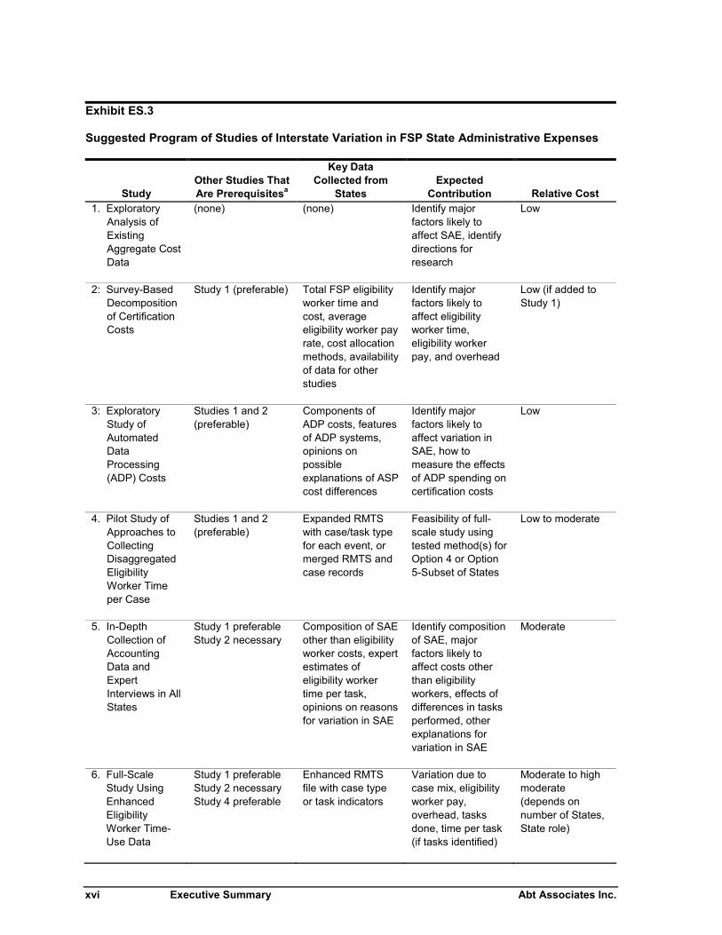
data—Option 4 or Option 5-Subset of States. Exhibit ES.3 summarizes the studies, theirprerequisites, their key data, their expected contributions to understanding of interstate variation inSAE, and their relative expected cost. In this exhibit, “low” cost means expected cost under$500,000; “moderate” cost means expected cost between $500,000 and $1,000,000; and “high” costmeans expected cost more than $1,000,000. The expectations are based on confidential estimatesprovided separately to FNS.
Study 1: Exploratory Analysis of Existing Aggregate Cost Data
This study would analyze existing aggregate cost data, as in Option 1 using reduced form difference-of-difference regressions. We view this as a relatively modest, low-cost first step that could provideimmediate insights and identify directions for future research. The primary focus would be on time-series regression analysis of certification costs (potentially using both narrow and broad definitions),but the scope could be expanded to include the costs of other functions. Extant FNS data and otherpublic databases would be used to construct explanatory variables. The study would attempt to modelthe relationship of certification costs to average eligibility worker pay, market pay for relatedoccupations, case characteristics, frequency of certification and recertification, and State fiscalconditions and budget constraints. The study would also identify persistent cost differences amongStates not explained by these factors. It would seek to relate FSP performance to SAE after takinginto account the known uncontrollables.
Study 2: Survey-Based Decomposition of Certification Costs
In this study, States would be surveyed to collect several types of data needed to conduct analysisbased on Option 2 and Option 5-National Averages. The survey would also gather data to clarify thefeasibility of more detailed analysis approaches. As discussed above, Option 2 would dividevariation in certification costs into three parts: eligibility worker time per case, eligibility worker pay,and “overhead”, i.e., the ratio of other certification costs to eligibility worker costs. Option 5-National Averages would disaggregate eligibility worker time per case as a function of case mix, taskfrequency, and intensity of effort relative to the task workload.
The study would combine the State survey data with existing data on SAE caseload characteristics,policy options, factor prices, and political, economic, and social conditions. The analysis wouldmodel the three elements of Option 2: eligibility worker time per case, eligibility worker pay, andoverhead. Additional analysis would implement Option 5-National Averages with the eligibilityworker time data and data on task frequency by case type from FNS sources. If data on eligibilityworker time by program combination were collected, the analysis specified under Option 3 would beimplemented.
The cost of this study would be low if it were added to Study 1, and the exploratory analysis ofaggregate data would help guide the analysis of the more disaggregated data and the data sought inthe survey. A State survey could also be combined with any of the other concepts described below.
xvi Executive Summary Abt Associates Inc.
Exhibit ES.3
Suggested Program of Studies of Interstate Variation in FSP State Administrative Expenses
StudyOther Studies ThatAre Prerequisitesa
Key DataCollected from
StatesExpected
Contribution Relative Cost1. Exploratory
Analysis ofExistingAggregate CostData
(none) (none) Identify majorfactors likely toaffect SAE, identifydirections forresearch
Low
2: Survey-BasedDecompositionof CertificationCosts
Study 1 (preferable) Total FSP eligibilityworker time andcost, averageeligibility worker payrate, cost allocationmethods, availabilityof data for otherstudies
Identify majorfactors likely toaffect eligibilityworker time,eligibility workerpay, and overhead
Low (if added toStudy 1)
3: ExploratoryStudy ofAutomatedDataProcessing(ADP) Costs
Studies 1 and 2(preferable)
Components ofADP costs, featuresof ADP systems,opinions onpossibleexplanations of ASPcost differences
Identify majorfactors likely toaffect variation inSAE, how tomeasure the effectsof ADP spending oncertification costs
Low
4. Pilot Study ofApproaches toCollectingDisaggregatedEligibilityWorker Timeper Case
Studies 1 and 2(preferable)
Expanded RMTSwith case/task typefor each event, ormerged RMTS andcase records
Feasibility of full-scale study usingtested method(s) forOption 4 or Option5-Subset of States
Low to moderate
5. In-DepthCollection ofAccountingData andExpertInterviews in AllStates
Study 1 preferableStudy 2 necessary
Composition of SAEother than eligibilityworker costs, expertestimates ofeligibility workertime per task,opinions on reasonsfor variation in SAE
Identify compositionof SAE, majorfactors likely toaffect costs otherthan eligibilityworkers, effects ofdifferences in tasksperformed, otherexplanations forvariation in SAE
Moderate
6. Full-ScaleStudy UsingEnhancedEligibilityWorker Time-Use Data
Study 1 preferableStudy 2 necessaryStudy 4 preferable
Enhanced RMTSfile with case typeor task indicators
Variation due tocase mix, eligibilityworker pay,overhead, tasksdone, time per task(if tasks identified)
Moderate to highmoderate(depends onnumber of States,State role)
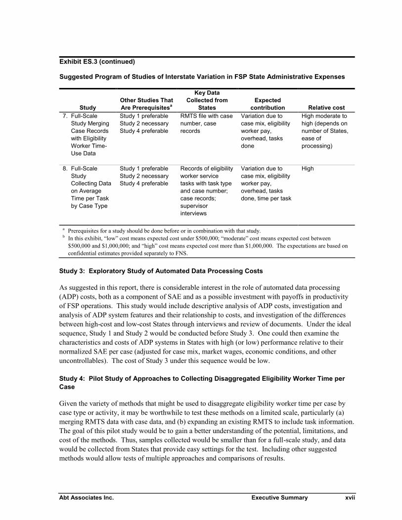
Abt Associates Inc. Executive Summary xvii
Exhibit ES.3 (continued)
Suggested Program of Studies of Interstate Variation in FSP State Administrative Expenses
StudyOther Studies ThatAre Prerequisitesa
Key DataCollected from
StatesExpected
contribution Relative cost7. Full-Scale
Study MergingCase Recordswith EligibilityWorker Time-Use Data
Study 1 preferableStudy 2 necessaryStudy 4 preferable
RMTS file with casenumber, caserecords
Variation due tocase mix, eligibilityworker pay,overhead, tasksdone
High moderate tohigh (depends onnumber of States,ease ofprocessing)
8. Full-ScaleStudyCollecting Dataon AverageTime per Taskby Case Type
Study 1 preferableStudy 2 necessaryStudy 4 preferable
Records of eligibilityworker servicetasks with task typeand case number;case records;supervisorinterviews
Variation due tocase mix, eligibilityworker pay,overhead, tasksdone, time per task
High
a Prerequisites for a study should be done before or in combination with that study.b In this exhibit, “low” cost means expected cost under $500,000; “moderate” cost means expected cost between
$500,000 and $1,000,000; and “high” cost means expected cost more than $1,000,000. The expectations are based onconfidential estimates provided separately to FNS.
Study 3: Exploratory Study of Automated Data Processing Costs
As suggested in this report, there is considerable interest in the role of automated data processing(ADP) costs, both as a component of SAE and as a possible investment with payoffs in productivityof FSP operations. This study would include descriptive analysis of ADP costs, investigation andanalysis of ADP system features and their relationship to costs, and investigation of the differencesbetween high-cost and low-cost States through interviews and review of documents. Under the idealsequence, Study 1 and Study 2 would be conducted before Study 3. One could then examine thecharacteristics and costs of ADP systems in States with high (or low) performance relative to theirnormalized SAE per case (adjusted for case mix, market wages, economic conditions, and otheruncontrollables). The cost of Study 3 under this sequence would be low.
Study 4: Pilot Study of Approaches to Collecting Disaggregated Eligibility Worker Time perCase
Given the variety of methods that might be used to disaggregate eligibility worker time per case bycase type or activity, it may be worthwhile to test these methods on a limited scale, particularly (a)merging RMTS data with case data, and (b) expanding an existing RMTS to include task information.The goal of this pilot study would be to gain a better understanding of the potential, limitations, andcost of the methods. Thus, samples collected would be smaller than for a full-scale study, and datawould be collected from States that provide easy settings for the test. Including other suggestedmethods would allow tests of multiple approaches and comparisons of results.
xviii Executive Summary Abt Associates Inc.
The cost of Study 4 would be low to moderate, depending on the number of approaches tested, thenumber of States, and the role of the States. Some States might be willing to take on some of the costof the test in order to have access to the results (e.g., training workers to complete new forms,processing the merge of RMTS and case records, etc.), while others might expect the researchers tocarry out all of the data collection and processing.
Study 5: In-Depth Collection of Accounting Data and Expert Interviews in All States
A logical follow-up to Study 2 would collect three kinds of data in each State: accounting data for thedecomposition of overhead, expert estimates of the eligibility worker time per task, and discussion ofthe reasons for variation in SAE. The accounting data would be collected to attempt thedecomposition of overhead by level (local/State), between labor and nonlabor, and breaking out keynonlabor costs such as rent. The estimates of eligibility worker time per task would be obtainedthrough interviews with key informants to permit implementation of the recommended version ofOption 5-All States. There would be an excellent opportunity to discuss the findings of studies ofSAE, both in general and with respect to each State individually. These discussions would help get“inside the black box” to understand the findings and suggest future directions for research. The costof such a study would be moderate; a low-cost version could be done if the data collection werelimited to 15 or fewer States.
Study 6: Full-Scale Study Using Enhanced Eligibility Worker Time-Use Data
This has the potential to be the least costly of the three approaches that appear to be feasible ways toimplement Option 4 or Option 5-Subset of States. In a representative group of States, the RMTS orpersonnel activity report would be modified to capture data on the type of case served, the task, orboth for each recorded event. Under one scenario, the researchers collaborate with the State tomodify the forms, and the State carries out the data collection and tabulates the data. Under the otherscenario, the researchers would implement the study. The State would approve the forms and supplythe sample frame, and the researchers would do the rest. It appears that the most feasible approach inthis scenario would be a telephone-based system, akin to a random-digit-dial survey. The cost ofStudy 6 would in five to seven States be moderate to high moderate, depending on who collects thedata.
Study 7: Full-Scale Study Merging Case Records with Eligibility Worker Time-Use Data
This approach also appears to be a feasible way to implement Option 4 or Option 5-Subset of States,and it would be less burdensome to individual workers than the alternatives for these options (Study 6and Study 8). In a representative group of States, researchers would collect and merge two data sets:RMTS or activity report data in electronic form with a case number for each event, and case recordsfor the same time period. Efforts for the study would include: designing the sample and analysis,securing State cooperation and access to data, obtaining and processing files, and analysis andreporting. Because of the use of case records in addition to RMTS data, this study would be morecostly than Study 6: the cost would be high moderate to high, depending on the number of States andthe ease of processing their data.
Abt Associates Inc. Executive Summary xix
Study 8: Full-Scale Study Collecting Data on Average Time per Task by Case Type
This study would essentially replicate the 1989 certification cost study, which was conducted in fourStates. Eligibility workers in selected offices would record each task for a specified period (such as amonth), including the type of task, the duration, and the case type or case number. Supplementarytime per task data might be collected from supervisors and support staff via interviews or surveys.Tests for differences in average time per task by case type would be conducted. Case records wouldbe analyzed to determine the frequency of the tasks and the relationship of case characteristics to taskfrequency. Data from the States with the in-depth data collection would be combined with aggregatedata for all States (SAE, case characteristics, economic conditions, etc.) for an analysis combining theapproaches of Options 4 and 5. The cost of Study 8 would be the highest of all eight studies.

xx Executive Summary Abt Associates Inc.
Abt Associates Inc. Introduction 1
PART I: INTRODUCTION AND CONCEPTUAL FRAMEWORK
Chapter 1
Introduction
In September 2007, the Food and Nutrition Service (FNS), U.S. Department of Agriculture (USDA)awarded to Abt Associates Inc. the Feasibility of Assessing Causes of State Variation in Food StampProgram (FSP) Administrative Costs Study (hereafter the Feasibility Study).5 The purpose of thestudy is to develop a menu of approaches for better understanding how and why State administrativeexpenses (SAE) vary between States.
The Feasibility Study addresses two sets of research questions: issues of the data sources to be used,and alternatives for analyzing and explaining variations in administrative expenses. In particular,
Is it possible to measure food stamp administrative expenses consistently enough acrossStates to credibly assess the degree of variation? If it is possible, what are the alternativeways to measure such expenses? Are new data required? If so, what level of effort would berequired and what challenges would need to be addressed to obtain such data?
Can the causes of variation in State food stamp administrative costs be explained in theabsence of experimental design? Why or why not? If so, what are the alternativeapproaches, and what are the advantages and disadvantages of each? Which approach isrecommended and why?
These questions are interrelated. The types of data required depend on the methods to be used, andthe feasible methods depend on the feasible data sources.
The remainder of this chapter presents some background on FSP costs, the research questions for thestudy, an overview of the strategy for explaining variation in SAE, and the data sources and methodsused in this study. The balance of this report expands on many of the points first touched on here.Finally, at the end of this chapter, we discuss the structure of the balance of the report.
Food Stamp Program Costs
The FSP provides assistance to low-income households so that they can purchase an adequate supplyof nutritious food. The FSP is the largest of the 15 domestic food and nutrition assistance programsadministered by the US Department of Agriculture’s Food and Nutrition Service (FNS). The FSPserved 26.5 million people in an average month in Fiscal Year 2007, for a total Federal cost of $33.2billion, of which $30.4 billion were for food stamp benefits (FNS, 2008a).
5 On October 1, 2008, the Food Stamp Program will change its name to the Supplemental NutritionAssistance Program (SNAP).
2 Introduction Abt Associates Inc.
The FSP is jointly administered by the Federal government and the States.6 The Federal governmentsets the basic program parameters and pays for all benefits. State governments choose programoptions from among those allowed by Federal statute and FNS regulations, and administer theprogram. Ten States devolve to their county governments the operation of the FSP, with varyinglevels of State supervision. The principal FSP administrative activities are certifying initialeligibility, updating and recertifying eligibility, issuing benefits (currently via electronic benefitstransfer/EBT cards), and fraud control (investigating possible fraud and recovering overpayments).In addition, the FSP provides employment and training (E&T) and nutrition education (FSNE)services to eligible persons.
The Federal government and the States split the cost of administration; where the FSP is county-administered, county governments share the non-Federal expenses with the State. Administrativecosts at the local and State levels are known formally as State Administrative Expenditures (SAE).These expenses are considerable. In FY2007, SAE totaled $5.5 billion, representing 17 percent oftotal FSP expenditures (FNS, 2008a). This is equivalent to $469 per participating household.7 Wediscuss the determinants of SAE in the next chapter. Here, we note that per-case SAE varies widelyacross the States. The range in FY2007 was from $169 in South Carolina to $1,169 in California,more than a nearly seven-fold difference. SAE per case also varies over time: between 1989 and2005, the average administrative expenditure for the nation (in 2005 dollars) ranged from $346 and$657 per household (Logan, Kling and Rhodes, 2008).
Administrative costs have a greater share of total program costs in the FSP than in several otherhuman service programs, including the Temporary Assistance for Needy Families (TANF) andUnemployment Insurance (UI) programs, but less than in others, such as adoption assistance andfoster care, according to a recent General Accountability Office study (GAO, 2006). The FSP alsospends a greater percentage of funds on administrative costs than the Earned Income Tax Creditprogram, according to another recent study (Isaacs, 2008). Because of differences in programs and inthe definition of administrative costs, such comparisons represent a starting point, not a basis forconclusions, regarding the question of whether the FSP is more or less efficient than other similarprograms (as pointed out by the GAO report). Nevertheless, these comparisons highlight the need tounderstand what drives the differences between low-cost and high-cost States, and whether there arelessons for improving the efficiency of the FSP.
6 For the purposes of this report, references to “States” include the 50 States and the District of Columbia butexclude Guam and the Virgin Islands, which are not expected to be part of a cost study because of theirunique circumstances.
7 This estimate is computed as the ratio of total SAE to average monthly food stamp households. The actualnumber of unique households participating in the FSP during a year is more than the average of themonthly counts, but the annual unique count is not regularly reported. The annual cost per FSP householdas defined above is equal to 12 times the average monthly cost per FSP household, and thus the annual andmonthly cost per household are perfectly correlated.
Abt Associates Inc. Introduction 3
Federal and State Perspectives on Variation in AdministrativeExpenses
Both Federal and State officials should be interested in the sources of variation in FSP SAE. At theFederal level, SAE is a large portion of FSP costs and a potential target for cutting federalexpenditures. FNS generally pays half of the cost but States largely determine the level of SAEthrough their decisions about staffing, contracting, and other spending.8 Thus, in considering thepotential to reduce Federal expenditures for SAE, FNS and Congress might reasonably ask whetherthe wide variation in FSP SAE is evidence of potential cost savings if all States would adopt thestrategies of the low cost States.
In the next chapter, we develop an integrated conceptual model of the determinants of FSP SAE. Thediscussion in that chapter suggests that it is useful to conceptualize the sources of variation in SAE asfalling into two groups.
1. Uncontrollables: These are sources of variation that are beyond the control of the State.Such uncontrollables would include input prices (e.g., prevailing local wage rates, prevailinglocal rents, computer costs); they also include local demographic and economic conditions,which are a major source of variation in the size of the FSP caseload and its composition.The more interstate variation in FSP SAE is due to uncontrollables, the smaller is the scopefor cost savings.
2. Controllables: These are sources of variation that are within the control of the State. Suchcontrollables include FSP policies that affect which SAE tasks must be done (e.g., quarterlyor semiannual reporting of earnings) and target service levels. More outreach, shorter waitingtimes for clients in offices and for processing of applications, more help in completingapplications, and higher levels of accuracy all require more resources. In addition, manyaspects of management structure are controllable and potentially affect SAE (e.g., State vs.county administration; use of call centers, investment in computer technology). The moreinterstate variation in FSP SAE is due to controllables, the larger is the scope for cost savings.
This discussion suggests that a key goal of any study of FSP SAE should be to establish how much ofthe variation is due to controllables. The discussion in Chapter 3 focuses on outlining models of FSPSAE that are estimable with obtainable data. These models would allow FNS to divide the variationbetween controllable and uncontrollable sources.
8 There are several exceptions to the 50-50 split of SAE between FNS and the States. Starting in FY1999,the Federal share of certification costs has been reduced to offset the FSP share of common costs includedin each State’s TANF grant, as required by the Agricultural Research, Extension, and Education ReformAct of 1998 (AREERA, P.L. 105-185). State “reinvestment” in lieu of financial sanctions is not matched.FNS pays 75 percent of costs for administering the FSP on Indian reservations. In addition toreimbursement of the Federal share of SAE, FNS pays bonuses to States with top or most improvedperformance in payment accuracy, program access, and timeliness of certification.
4 Introduction Abt Associates Inc.
In addition, Federal and State officials may be interested in the effects of specific policy andmanagement choices.9 Does adopting semi-annual reporting cut SAE? By how much? Are county-administered systems more expensive? By how much? Do investments in computer technology leadto long term savings in total SAE? In addition to strategies for explaining interstate variation in FSPSAE (and the extent to which it is due to uncontrollables and controllables), this document considersdata and analysis strategies for estimating the cost implications of specific policy and managementchoices.
Purpose and Research Questions
This report has two purposes: (1) to identify and compare data sources that researchers could use to“credibly assess the degree of variation” in FSP SAE, and (2) to identify and assess potentiallyfeasible non-experimental approaches to analyzing these data.
Feasibility of Obtaining Suitable Data for Analysis of Variation in SAE
In approaching the first purpose, we expanded on the research questions posed by FNS, as discussedbelow.
Is it possible to measure food stamp administrative expenses consistently enough acrossStates to credibly assess the degree of variation?
There are two basic issues posed by this question. The first is whether it is possible to obtainmeasures of expenses in all States (or a sample) that are consistent, i.e., that are measured in the sameway. If the measurement of costs is different across States, this could introduce random variation(noise) or it could bias comparisons. As discussed later in this report, “measurement” may beobtaining data from FNS files or State information systems, or conducting new data collection. Thesecond issue, not stated but implicit in the question, is whether it is possible to measure expenses insufficient detail to allow not only description of variation but also explanation of it. As becameclear in the assessment of analytic techniques, more detailed information is useful because it allowsmore “apples to apples” comparisons, and because analysis strategies can use more detailedinformation to focus on variation in components of costs, such as direct service staff time versussupervision versus nonlabor costs.
If it is possible, what are the alternative ways to measure such expenses? Are new datarequired?
We identified three basic ways that SAE can be measured, in ascending order of cost and burden.First, comparisons can use the State-level expenditures reported to FNS. This approach requires nodata collection, and indeed Abt Associates already has created and used an analysis file of these datafor 1989 through 2005 for a study funded by the USDA Economic Research Service (Logan, Kling,and Rhodes, 2008). Second, one could collect existing expenditure data from State accountingsystems. These systems include not only the purely financial data that directly support the claims to
9 See GAO (2006, p. 36) “(T)here are opportunities available to the federal government to assist state andlocal governments in better identifying and implementing cost-saving initiatives that also ensure accurateand timely provision of benefits and services. However, minimal information is available on whichopportunities are most effective and what any actual cost savings might be.”
Abt Associates Inc. Introduction 5
FNS but also the time measurement systems and other data systems that are used to allocate costsbetween the FSP and other programs. This approach would require cooperation from Stateaccounting staff, but it would not pose any burden on local program staff. Finally, one could conductprimary data collection, in order to assure that the data were sufficiently detailed and comparableacross States. This would require responses from local and State program staff (such as surveys ortime studies), and also from accounting staff (for payroll and overhead costs).
What level of effort would be required and what challenges would need to be addressed toobtain such data?
These questions apply both to the collection of existing expenditure data and to primary datacollection on administrative expenses. The underlying issue is that FNS needs to know whether astrategy is feasible and whether it is worthwhile—that is, whether the effort of collecting data can bejustified by the gain in the quality of data and the ability to draw conclusions from comparisons. Thelevel of effort includes both the effort that FNS would fund (through a research contract) and theeffort for the States and their staff to cooperate and provide the data. Other than contractor effort andburden on States, potential challenges for collecting existing data depend on the systems of accountsand other categories in which data are organized, the form in which the data are maintained (e.g., arerecords archived after a certain period?), and restrictions on access to records containing non-publicinformation. Challenges for primary data collection include research design, pretesting, training andsupervising data collectors, building sample frames (if applicable), conducting data collection, anddealing with nonresponse. An issue for collecting existing and primary data is that, where countiesoperate the FSP under State supervision, cooperation of counties is needed, and records may beavailable only at the county level.
Feasibility of Non-Experimental Methods for Explaining Variation in SAE
The first research question for considering analytic methods to explain variation in SAE is:
Can variations in State food stamp administrative costs be explained in the absence ofexperimental design?
Experiments are the “gold standard” of social science, but in this context an experiment is notfeasible, as explained below.
A well-designed experiment assures that the treatment and control groups differ systematically onlyin the interventions being explored, so that differences in outcome can be attributed to the treatmentor conditions under study, and our uncertainty about the results can be precisely expressed as afunction of sampling and measurement error. In public policy studies, experiments are used to testthe effectiveness of interventions or changes in policy with random assignment at the individual,group, or site level.
Attempting an experiment with random assignment of policies at the State level poses two majorproblems. (“Policies” may be specific rules or practices, or more global choices such as decentralizedversus centralized processing of cases.) First, obtaining the agreement of States to set their policies asspecified by the evaluation’s “coin toss” or other random outcome would be difficult if notimpossible. Second, with at most 25 States in each group, the likelihood of significant and relevantdifferences other than the specified intervention or policy is high and the power to detect differences
6 Introduction Abt Associates Inc.
in a simple comparison between groups may be low. For example, the cost impact of allowing on-line applications would depend on the rate of new applications, which will vary with Statedemographics and economic conditions. With a small sample, there is a substantial probability thatthe treatment group might have significantly more (or less) frequent new applications and thus more(or less) savings in the overall certification cost per case. In a non-experimental study, of course,State differences may in fact contribute to policy choices, so this issue is not unique to experiments.
Furthermore, there are many factors under the control of State agencies that may contribute tovariation in food stamp SAE among States. A large number of experiments would be needed to testall of the policy options and alternatives for structuring operations. Each experiment would need toassure that there is no significant difference between groups in policies that might affect the outcome,other than the policy being tested. Finally, policy effects may interact, and the most effectivecombinations may be unknown, thereby adding another dimension of complexity. This issue, too, isone common to both experimental and non-experimental studies.
An experimental design might be used within a State to test the effects of policy or managementchoices on administrative costs. Such an experiment would allow variation in a limited set of choicevariables across counties while holding constant other conditions that vary between but not withinStates (such as the effectiveness of the computer system). Issues for conducting such an experimentwould include: gaining cooperation of county agencies, implementing policies that vary by county,measuring costs accurately at the county level, and generalizability of the results to other States. If anexperimental design is not feasible but other conditions are favorable, a non-experimental study mightexamine the relationship of varying policies and practices to administrative costs (for example, arecertification costs higher or lower when workers specialize on intake versus ongoing casemanagement, relative to a generalist staffing model?).
Thus, while experimental methods have higher internal validity, nonexperimental methods are morelikely to be useful for understanding variation in SAE. The fundamental weakness of non-experimental approaches is the risk of selection bias. States differ both in the policies they choose(the controllables) and in factors that are beyond their control (the uncontrollables). If States choosepolicies in response to uncontrollable conditions, and those conditions also affect the outcome ofinterest (in our case SAE), we must be aware of the role of these conditions and take them intoaccount in the analysis; otherwise, we will incorrectly attribute their effects to the policies of interest.For example, States with high wage rates for eligibility workers might be more likely to adoptpolicies that reduce eligibility worker burden, such as simplified (semi-annual) reporting of incomeand household circumstances. Unless one adjusted statistically for differences in wage rates, onemight conclude that costs are higher when simplified reporting is used, or that simplified reportingmakes no difference in costs, when in fact this procedure is helping States to keep costs down. Thegreatest problem arises with unknown uncontrollables that are related to policy choices andoutcomes, because we cannot include these factors directly in the analysis. (Time series analysistechniques can be used to control for unknown State characteristics that may be related to policychoices, as discussed in Chapter 3.) In addition, if the controllable factors (policies and procedures)are highly correlated with uncontrollable factors (such as the local economy), their effects cannot beseparated.
An additional challenge for non-experimental approaches is the large number of potential factors formodeling variation in SAE. The “uncontrollables” include case characteristics, caseload dynamics(entry and exit rates, volatility of employment and earnings, etc.), some State and local agency
Abt Associates Inc. Introduction 7
characteristics (scale, scope,), and pay rates in relevant labor markets. The “controllables” includepolicies and procedures, investments in systems and training, actual pay rates for workers, and use ofcontractors. When there are many potential variables, it becomes more difficult to estimate theireffects, particularly if “uncontrollables” and “controllables” are highly correlated. This is theproblem of collinearity. As noted above, however, the large number of potential factors affectingcosts is also a challenge for any experimental study.
The limitations of a non-experimental study are less problematic when the purpose is exploratory, i.e.,if FNS seeks to examine the conditions associated with variations in costs, without expecting adefinitive answer about what causes variations in costs. The information gained from an exploratorystudy could generate hypotheses that are worth testing formally. Also, a non-experimental studywould be less prone to bias if it focused entirely on uncontrollable sources of cost variation througha “reduced-form” approach (assuming that all decisions on controllables are driven ultimately byuncontrollables). However, this reduced-form approach would not provide any information on theeffects of policies. Last, the problems of non-experimental designs can be reduced by the choice ofanalytic techniques. If the theoretical model of aggregate costs has too many variables or significantunknowns, the costs can be disaggregated into simpler and more complete models. Bias in estimatingthe effects of State choices can be avoided by analytic methods that control for unmeasured variablesassociated with State choices.
As discussed in this report, there are a number of possible non-experimental approaches that canprovide insights into the sources of variation in food stamp SAE. The degree of confidence in theseinsights will depend on risk of selection bias and collinearity, the sensitivity of results to theassumptions, and the quality of the data. Thus, we reframe the research questions regarding analyticmethods as:
How well can variation in State food stamp administrative costs be explained with non-experimental methods? What are the alternative approaches, and what are the advantagesand disadvantages of each? Which approach is recommended and why?
To answer the first question, we must address the second. We broke it down into the followingquestions:
What are the alternative conceptual frameworks for explaining variation in SAE?
What data and analytic methods could be used to apply these frameworks?
What are the potential study designs, their data requirements, and their theoretical advantagesand disadvantages?
What are the implications of the data assessment (addressing the first study objective) for thefeasibility and relative merits of the potential study designs?
This report addresses these questions and provides recommendations for a program of study oninterstate variation in SAE. We draw on existing literature regarding administrative cost issues in theFSP and related programs, on established principles of non-experimental design, on our priorexperience in studies of the FSP and related programs, and on the data collection for the study. Thebasic strategy for explaining variation in SAE and the data sources for the report are described below.
8 Introduction Abt Associates Inc.
An important issue for this study was that total SAE for the FSP includes the costs of a substantialnumber of different functions, each with its own set of tasks and inputs. Thus, to explain the variationin total SAE, one must analyze each function. A complete feasibility assessment for analyzing all ofthe FSP functions would be a very complex and extensive document, and was beyond the scope ofthis study.
For this study, we prioritized our assessment by assuming that certification is the most importanttheoretical category. Certification costs—as labeled in State reports—represent three-fifths of allSAE (as discussed in Appendix A). We define certification costs more broadly for this study, toinclude in principle all of the direct and indirect costs of determining eligibility and maintainingcases. (This definition is discussed in Chapter 5.) Certification policy gives States many options thatmay affect costs. Certification is primarily carried out by local agency staff, particularly eligibilityworkers, so we devoted the most attention to the data and methods to analyze variation in these costs.We also assumed that data processing costs are another area of interest, mainly because of thepotential trade-offs between eligibility worker costs and automated data processing costs. Weacknowledge that services to clients other than certification (such as nutrition education, employmentand training, and fraud control) are important FSP functions, but different frameworks are needed tostudy variation in their costs. These frameworks can build on the concepts and approaches in thisreport.
Key Themes of This Report
A major theme of this report is that there is an interplay between analytic assumptions, datarequirements, analysis strategies, and the strength of conclusions that can appropriately be drawn.Analyses using easily available data require strong assumptions and will support only weak—thoughstill potentially insightful—conclusions. Additional data will allow more robust approaches andstronger conclusions. Our assessment of these approaches and trade-offs is guided by ourunderstanding of the importance of these issues to FNS and the States, and our awareness of theconstraints on FNS’ research budget. Following the development and assessment of approaches anddata, the final chapter of the report sketches several attractive strategies.
Another key theme of this report is a focus on the use of existing data, including the States’ reportedadministrative expenses for the FSP and supporting data from time measurement and accountingsystems. The key time measurement process in most States is a “random-moment time study”(RMTS) in which randomly selected workers record their activities and the program they are workingon at randomly selected times. Such data are much less burdensome and costly to collect than new,primary data, which require responses from large numbers of busy people to assure statistically validestimates. Moreover, State accounting systems maintain multiple years of data that could supportlongitudinal analysis, whereas primary data collection on the scale that would be needed for a studyof SAE would at most be feasible on a one-time basis. (Background on State accounting and costallocation systems is provided in Appendix B.)
On the other hand, we identify a number of known limitations and uncertainties about the existingdata. The most important limitation is that the ideal level of detail on costs does not appear to bewidely available and would not be feasible to obtain. However, we suggest ways to use more feasibleresearch strategies to improve over the simplest approach: time series of cross-sections analyses ofaggregate SAE cost data as a function of controllables and uncontrollables. There appear to be some
Abt Associates Inc. Introduction 9
inconsistencies in definition, measurement, and cost allocation across States and over time that posesome constraints for analysis, but these are far from fatal to the suggested approaches. There areseveral uncertainties about the structure and scope of existing cost data, but these could be readilyaddressed through a survey of States. There is a wealth of strong national databases for manypotential explanatory variables, but there are some notable limitations with respect to workeractivities, price variation for inputs other than labor, State fiscal conditions, and FSP procedures andoperating characteristics.
Data Sources for This Report
For this study, we reviewed a range of published reports on administrative costs in the FSP andsimilar programs, as documented in the references of both memoranda. While we did not conduct asystematic literature search, we identified relevant publications through key agencies’ web sites(FNS, USDA Office of Inspector General, Government Accountability Office, and Department ofHealth and Human Services) and through our prior research experience.
We also conducted semi-structured interviews with officials at FNS Headquarters, four regional FNSoffices, and the Department of Health and Human Services to gather information about five maintopics:
the comparability of reported administrative expenditures among States,
the availability of usable information on the composition of administrative expenditures fromStates,
the feasibility of collecting and analyzing client information system data on case openingsand changes,
the availability of data on State budgets for administering public assistance programs, and
respondents’ views on the reasons for variation in administrative costs across States.
The interview topic guides for these Federal interviews are provided in Appendix C.
We selected and recruited four States for telephone interviews to gather further information aboutcost reporting, available data, challenges of collecting data for expenditure analysis, and possibleexplanations for variation in SAE across States and over time. The States, selected to represent arange on several dimensions (size, administrative cost per household, county- versus State-administered, and FNS region), were Nevada, New Mexico, North Carolina, and Pennsylvania. TheStates and their characteristics are shown in Exhibit 1.1. The topic guide for these State interviewsappears in Appendix D. The major topics were:
What types of local office employees are involved with FSP certification and related tasks,and what are their other functions?
How are local office worker costs for the FSP measured?
How are other key administrative costs for the FSP measured and allocated?
What are the major challenges in measuring and reporting FSP expenses, and how do theyaffect the reporting of SAE?
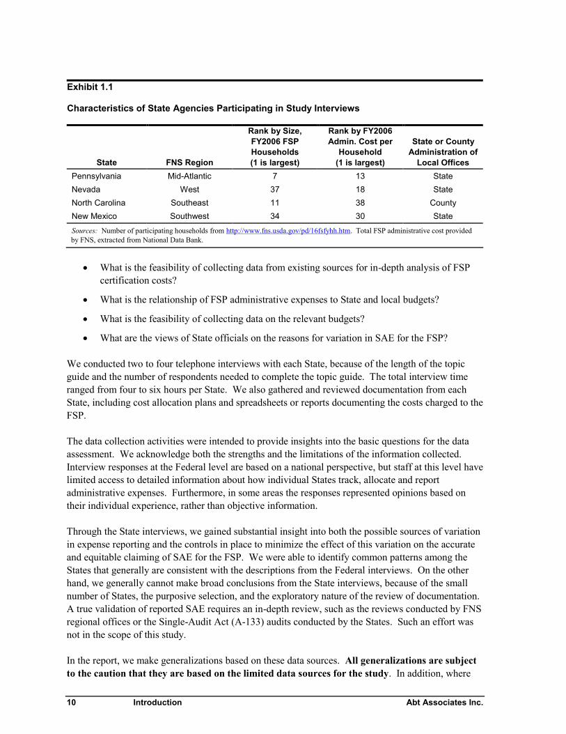
10 Introduction Abt Associates Inc.
Exhibit 1.1
Characteristics of State Agencies Participating in Study Interviews
State FNS Region
Rank by Size,FY2006 FSPHouseholds(1 is largest)
Rank by FY2006Admin. Cost per
Household(1 is largest)
State or CountyAdministration of
Local Offices
Pennsylvania Mid-Atlantic 7 13 State
Nevada West 37 18 State
North Carolina Southeast 11 38 County
New Mexico Southwest 34 30 State
Sources: Number of participating households from http://www.fns.usda.gov/pd/16fsfyhh.htm. Total FSP administrative cost providedby FNS, extracted from National Data Bank.
What is the feasibility of collecting data from existing sources for in-depth analysis of FSPcertification costs?
What is the relationship of FSP administrative expenses to State and local budgets?
What is the feasibility of collecting data on the relevant budgets?
What are the views of State officials on the reasons for variation in SAE for the FSP?
We conducted two to four telephone interviews with each State, because of the length of the topicguide and the number of respondents needed to complete the topic guide. The total interview timeranged from four to six hours per State. We also gathered and reviewed documentation from eachState, including cost allocation plans and spreadsheets or reports documenting the costs charged to theFSP.
The data collection activities were intended to provide insights into the basic questions for the dataassessment. We acknowledge both the strengths and the limitations of the information collected.Interview responses at the Federal level are based on a national perspective, but staff at this level havelimited access to detailed information about how individual States track, allocate and reportadministrative expenses. Furthermore, in some areas the responses represented opinions based ontheir individual experience, rather than objective information.
Through the State interviews, we gained substantial insight into both the possible sources of variationin expense reporting and the controls in place to minimize the effect of this variation on the accurateand equitable claiming of SAE for the FSP. We were able to identify common patterns among theStates that generally are consistent with the descriptions from the Federal interviews. On the otherhand, we generally cannot make broad conclusions from the State interviews, because of the smallnumber of States, the purposive selection, and the exploratory nature of the review of documentation.A true validation of reported SAE requires an in-depth review, such as the reviews conducted by FNSregional offices or the Single-Audit Act (A-133) audits conducted by the States. Such an effort wasnot in the scope of this study.
In the report, we make generalizations based on these data sources. All generalizations are subjectto the caution that they are based on the limited data sources for the study. In addition, where
Abt Associates Inc. Introduction 11
we found conflicting evidence or heard differing views on a topic, we note this as an area ofuncertainty. The discussion of issues for future research reflects the limitations of our informationand the important areas of uncertainty.
Organization of this Report
The balance of this report provides relevant background, defines a series of possible researchapproaches and specific options, assesses the potential data sources, and assesses the feasibility of theoptions. The report is organized in three sections, each of which we describe below.
Part I of this report, the introduction and conceptual framework, includes this chapter and the threesubsequent chapters. We describe potential approaches to comparisons of SAE and analysis of thesources of variation, both in general and in relation to specific policy and management choices. Wepresent our conceptual framework and potential research approaches before discussing data sourcesbecause the data requirements depend on the analysis approach. Chapter 2 defines the three ways thatSAE may be decomposed, leading to the definition of four components of variation in SAE: inputprices, case mix, tasks per case, and inputs per task. The chapter then presents a conceptual model ofhow these components are determined. Chapter 3 presents a series of general analysis strategies,starting with a comprehensive but highly data-intensive approach and then presenting alternativestrategies that simplify the data requirements. In Chapter 4, these strategies are translated intospecific study designs, each of which consists of an analysis strategy, a set of data requirements, andone or more potential data sources.
Part II assesses the data sources for these study designs. The primary focus is on the availability andquality of data to analyze SAE at various levels of disaggregation, and the implications for thefeasibility of the proposed study designs. Chapter 5 examines the issue that is fundamental to anyattempt to explain variation in SAE: the extent to which reported SAE is comparable across Statesand over time. Chapter 6 explores the possible sources for analyzing the most important input forFSP administration: eligibility worker time, compensation and costs. In Chapter 7, we assessstrategies and data sources for decomposing reported expenses other than eligibility worker costs.Analysis of SAE requires data on the explanatory variables at the goals, policy, management, andpopulation levels; Chapter 8 assesses the availability and quality of data on these variables.
Part III presents our conclusions about the feasibility of explaining variation in SAE for the FSP. InChapter 9, we summarize the findings and present our recommendations for a suggested program ofresearch. This chapter categorizes the suggested studies on a scale of low to high expected costs.
Following the text, we provide references and background information in appendices. Appendix Apresents supplementary background information on FSP administration. To help the readerunderstand the nature of SAE, this appendix describes the administrative functions, the compositionof SAE, and the roles of local and State agencies. Appendix B summarizes the rules and systems foraccounting, allocation, and reporting of SAE. These rules and systems define SAE in practice and, asdiscussed in Part II, have important implications for the strengths and limitations of the data availableto analyze SAE at the accounting, case, and task levels. This appendix includes the form anddefinitions used in State reporting of SAE to FNS. Appendices C and D provide the interview guidesused to collect data for this study.

12 Introduction Abt Associates Inc.
Abt Associates Inc. Perspectives for Comparing Expenditures for the FSP 13
Chapter 2
Perspectives for Comparing State AdministrativeExpenditures for the FSP
This report’s consideration of feasible strategies for understanding variation in FSP SAE is built on aconceptual model of the components of FSP SAE and their determinants. This chapter develops thatconceptual model and its implications.
Decomposing FSP SAE
To understand our approach to FSP SAE it is useful to decompose FSP SAE in three ways: an“Accounting Decomposition”, a “Case Decomposition”, and a “Task Decomposition”. They aresuccessively finer and more insightful conceptual approaches. While none of these decompositionscan be directly estimated, we discuss in Chapter 3 how we might use available data to approximatethem.
Accounting Decomposition
By definition, the total State Administrative Expenditure for the FSP in a given period of time for agiven State is the sum of expenditures for all items purchased:
(2.1) j
jjj XpSAEFSP _
where j indexes every line in the State’s payroll and accounts payable detail file,10
X is the number of units of the input purchased,p is the price per unit paid for the input, and is the FSP share of the cost of the input.
Each term should have a superscript for State and time period. We suppress those subscripts forclarity. In this formulation, inputs are defined quite specifically, such as hours of an individual entrylevel eligibility worker, hours of the State Food Stamp director, or square feet of rental space at aspecific office).11 The unit prices of input are also specific, e.g., the fully compensation per hour foran entry level eligibility worker, including salary, fringe benefits, and taxes; or per-square foot rent ona particular office.
10 As noted in Chapter 1, county governments administer the FSP in some States. For simplicity, we refer inthe text to the “State” payroll or actions taken by the “State”, regardless of whether the State is directly orindirectly administering the FSP.
11 The definition of a unit of an input can vary, depending on the context. For example, workers may betypically paid on a biweekly basis. Thus, the accounting system shows the purchase of a unit of two weeksof work. With other data sources, smaller units of worker time can be defined. Similarly, the lease for acomputer may be a single annual payment, but its usage may be measured in much smaller units.
14 Perspectives for Comparing Expenditures for the FSP Abt Associates Inc.
The quantity and price terms are relatively straightforward. The FSP cost share () warrantsadditional discussion. FSP administrative expenditures at the State and local levels represent acombination of FSP-specific and shared activities. For FSP-specific activities, the entire cost ispassed to FSP SAE and we set to 1.0.
However, many activities affecting the FSP are shared. For example, the State FSP agency usuallyadministers Temporary Assistance for Needy Families (TANF), Medicaid eligibility, State cashassistance programs, and a variety of other programs of assistance for persons with low incomes.Thus, there are shared administrative activities at the State level and at the local level (overallmanagement, budget and finance, personnel, information systems, and so forth). To the extent thatthese activities represent fixed costs (at least within a certain range of combined caseloads), the FSPshare () will be lower in States where other programs are larger in relation to the FSP, particularly if those programs serve the same clients.
In addition, individual clients often participate in several programs at the same time. For example,most TANF and SSI recipients are categorically eligible for the FSP and Medicaid. Thus, manyactivities for FSP-TANF cases (e.g., taking the initial application, some aspects of renewal andredetermination) are intrinsically joint; i.e., a single action benefits multiple programs. As we discussin detail in Appendix B, federally approved cost sharing rules are used to assign a share of these coststo the FSP (and to the other programs). Thus, both the case mix and the State-specific cost-sharingrules will affect the FSP share. Individuals apply for SSI at an SSA office, where they can also applyfor the FSP. SSI recipients can jointly apply for the FSP and Medicaid at FSP offices. For SSIapplicants and recipients, the average FSP cost per case depends in part on how often thesehouseholds apply for the FSP through the SSA office rather than the FSP office. 12
This accounting perspective can be defined exactly. The index i includes every unique line in theState’s accounting system—each paycheck to each employee, every rent check, every payment to anoffice goods supplier. In this conceptualization, every transaction has a unique quantity, price, andshare allocated to the FSP.
Any attempt to use this approach in applied work would almost certainly want to aggregate individualtransactions to some higher level of aggregation. Such higher levels of aggregation might include:eligibility worker labor, supervisor labor, rent, computer systems, and “overhead” (i.e., the remainingcosts that are not included in separate categories). Equation 2.2 rewrites Equation 2.1 in terms of Kbroad types of purchases (indexed by k).
(2.2)
K
kkkk XpSAEFSP
1
_
12 Approximately 27 percent of FSP households participate in the Supplemental Security Income (SSI)program (Wolkwitz, 2007). If a household applies for the FSP at an office of the Social SecurityAdministration (SSA), the SSA shares some of the cost of FSP certification. The extent of this cost-sharingis a function of the share of FSP applicants eligible for SSI, the SSA share of FSP applications for SSIhouseholds, and the relative effort of the SSA and the State food stamp agency in processing suchapplications. The SSI/FSP Combined Application Projects (CAP) are intended to reduce the proportion ofSSI households that apply at FSP offices and streamline these applications; both of these changes would beexpected to result in FSP cost savings or in the reallocation of FSP administrative resources to other uses.
Abt Associates Inc. Perspectives for Comparing Expenditures for the FSP 15
where k is the input category,X is the total quantity of the inputs in the category purchased,p is the average price per unit paid for the inputs in the category, and is the average FSP share of the cost of the input.
We emphasize that the prices and FSP shares are averages over the inputs in the category k. At such ahigher level of aggregation, the mapping to actual financial systems is no longer exact. Each categoryis an aggregate of multiple inputs (e.g., different levels of experience of eligibility workers), eachwith its own price and varying in their cost shares. Given such an aggregation, an analyst will need toexplain how price, quantity, and cost sharing fraction are defined and how they combine to give totalFSP_SAE. In particular, the appropriate definition of quantity is not necessarily a simple sum whenthe inputs in a category are heterogeneous. For example, five hours of a more experienced workerwould be expected to produce more than five hours of an entry-level worker. This distinction isespecially important because turnover among eligibility workers varies substantially across andwithin States, according to experts interviewed for this report.
One natural approach would proceed as follows. Set the FSP share, , to the average share within thegroup; set the price to some observable market price (e.g., a cost index for local labor), and define thequantity such that the product of cost-share, price, and “quantity” equals the total SAE for everythingin this aggregate. Option 2 in Chapter 4 describes this approach in more detail.
This model leads naturally to a decomposition of FSP SAE in terms of the relative importance ofdifferent inputs. How do States vary in the share of FSP SAE going to eligibility workers, otherfront-line workers, supervisory staff, computer systems, and overhead (above the office level)? Italso leads naturally to decompositions in terms of variation in input prices (e.g., eligibility workerwages and rent are likely to be higher in more urban States).
Case Decomposition
It is useful to think of inputs being expended on individual cases. We argued in Chapter 1 thatcaseload composition might affect per case FSP SAE. Some types of cases are less expensive (e.g.,TANF cases for which certification costs are shared with TANF and Medicaid, elderly householdswith stable circumstances) and some types of cases are more expensive (e.g., cases with morehousehold members, cases with earnings that have more frequent changes in income).13 We seek adecomposition that incorporates this source of variation.
Again, we develop this approach in two stages. First, work at the case level:
(2.3)
N
c jcjjcj XpSAEFSP
1,,_
where c denotes an individual case,N is the total number of cases, is the FSP share of costs for case c,p is the price of input j used for case c, andX is the quantity of input j used for case c.
13 See Chapter 6 for discussion of the special case type of households receiving disaster assistance under theFSP.
16 Perspectives for Comparing Expenditures for the FSP Abt Associates Inc.
Within the brackets we have the cost from case c. As in Equation 2.1, it is the sum over all lines inthe detailed accounts payable data, j, of the product of the quantity of the input for the case, the priceof the input and the FSP share of the input.
With ideal data, this approach would be almost exactly defined. In principle, it is possible to identifyhow much time each eligibility worker spends on each case. It would not be necessary to measuretime for all cases; instead, a random sample of cases could be selected, and all workers could beinstructed to report time spent on these cases. (This is an adaptation of a method, known as the “jobticket,” used in government accounting systems (DoD, 1995).14 This measurement could in principlebe extended to capture the use of other inputs (recording computer time, tracking postage formailings, etc.), but of course this measurement would be a great burden on the State agencies andtheir staffs. Moreover, some inputs would have to be treated as overhead and assigned in proportionto the use of inputs that are directly measured. For example, while the space used by an eligibilityworker can be measured and assigned a cost per square foot, that space is used to serve numerouscases. Furthermore, several workers may serve a case at different times. Thus, to assign the cost ofspace to an individual case, it is necessary to apply an allocation rule, such as the percentage of totalstaff time in the local office devoted to the case.
Again, at this level of aggregation, this approach is not useful. To arrive at a more usefulformulation, we again aggregate individual expenditures into groups (with index k). We alsoaggregate individual cases into G groups (with index g) such that each case belongs in exactly onegroup. Then, we can write FSP SAE as:
(2.4)
G
g kgkkgkg XpnNSAEFSP
1,,_
where ng is the fraction of the total cases (N) represented by case type g,X is the average quantity per case of the inputs in the category purchased,p is the average price per unit paid for the inputs in the category, and is the average FSP share of the cost of the input.
It is now useful to view the inner summation as referring to averages for cases of type g (thus the barsover the terms). For a given case type, per case costs are the sum over all (grouped) inputs, k, of theproduct of the average number of units of each input, X, the cost per input, p, and the average costshare of this input for this case type,
We note that, in principle, the number of “cases” in this formula includes households that interactwith the FSP but are not authorized to participate. Some households inquire about the FSP but don’tapply; others begin but do not complete the application process; others apply and are denied benefits.In practice, there is no routine source of counts of all households interacting with the FSP. Therefore,we will refer to the cost per authorized case (or household), while acknowledging that not all costs areincurred for these households.
14 In a job ticket system, each worker that spends time on a specific product records that time on a form that isphysically or virtually attached to the product. This system provides information on the cumulative laborcosts of all of the steps that go into producing individual items. (Department of Defense (DoD), 1995.)
Abt Associates Inc. Perspectives for Comparing Expenditures for the FSP 17
Again, an analyst may want to redefine quantity to align with the observed prices. The outersummation computes the weighted average cost per case across case types, where the share of casesof each type (ng) is the weight. The total FSP SAE is then the product of the total cases (N) and theweighted average cost per case.
The crucial insight of this approach is that some types of cases require more inputs than others. InChapter 1, we argued that a key analytic challenge in understanding variation FSP SAE is to estimatethe amount of variation remaining after we control for uncontrollables—input prices and case mix.Equation 2.4 incorporates these two key uncontrollables; and can therefore provide a conceptualframework for that exercise. The equation also points to potential State differences in the amount ofinputs per case for a given case type, reflecting State choices about the level of service (broadlydefined). We develop this idea in much greater detail—including how to apply it to available data—in our discussion of Options 3 and 4 in Chapter 4.
Task Decomposition
The “Accounting Decomposition” defined FSP SAE in terms of specific inputs. The “CaseDecomposition” defined FSP SAE in terms of specific inputs and individual cases. The “TaskDecomposition” attempts to define FSP SAE in terms of specific inputs, individual cases, and actualtasks performed. It attempts to provide a framework in which to answer the question: What do Statesactually do that generate administrative expenses?
We are motivated to adopt this “Task Decomposition” because beyond uncontrollables (i.e., inputprices and case mix heterogeneity), we believe that FSP SAE varies because of two other factors: (i)what tasks States do; and (ii) what resources States use to do those tasks. Each of these conceptsdemands further discussion.
What Tasks States DoWhen “tasks” are appropriately defined, it seems unlikely that all States do the same “tasks”. FNSregulations require States to achieve certain high level outcomes. Initial certification must becompleted within some time frame. Periodic recertification must be completed with some frequency.All actions must be completed with acceptable error rates.
Sometimes those actions are optional or waivable if a State adopts a specific policy. Thus, States mayrequire FSP participants to file quarterly status reports. Shifting to semi-annual reporting should cutthe effort to process status reports in half.15 At State option, categorical eligibility for the FSP can bedefined more or less broadly, within the boundaries set by FNS policy. Where categorical eligibilityis expanded, more households are exempt from FSP asset limits, and therefore the State less often hasto determine the value of household assets. We want a conceptual model that can help us to thinkthrough how such policy changes should affect FSP SAE. Such a model should help us to specifyempirical approaches that will allow us to understand how such policy changes should affect FSPSAE. Understanding the effect of such policy changes should be a goal of any study of FSP SAE.
Furthermore, the intensity of some tasks is a State option. There is only a minimal requirement foroutreach (i.e., encouraging eligibles to reply), for helping applicants to complete applications. There
15 This is a simplification, not taking into account program exit rates by month and other considerations.
18 Perspectives for Comparing Expenditures for the FSP Abt Associates Inc.
is no requirement for Food Stamp Nutrition Education. Our conceptual model should help us tospecify an empirical model that will help us to understand how such tasks affect SAE.
Finally, we believe it is useful to specify tasks much more finely in terms of outcomes. For example,an ideal model would distinguish applications processed nearly immediately vs. applicationsprocessed just before the FNS deadline vs. applications processed after the deadline. Similarly, anideal model would distinguish between actions performed without errors and actions performed witherrors. An ideal model would distinguish between applicants seen immediately vs. applicants seenafter a wait (e.g., of more than an hour) vs. applicants asked to come back because the eligibilityworker could not seem them at all on the scheduled day. When a task is defined this way, and whenthe type of case is sufficiently specific, the input requirements are far better defined.
As we discuss in detail in the next section, this finer definition of a “task” is crucial for thinking abouthow State budget decisions affect the decisions of State FSP leadership and ultimately what happensin FSP offices and the services received by (current and potential) FSP participants. When State FSPSAE budgets are cut or when caseloads rise but State FSP SAE budgets do not (or in States withhistorically lower FSP SAE funding), something happens. Perhaps to some extent State employeesabsorb the extra work by putting in more effort. More likely, some tasks go undone, either at thedirection of State managers via explicit policy changes or through “triaging” decisions made at lowerlevels of the agency. There is less outreach, less help completing applications, less NutritionEducation. In addition, time on each broadly defined tasks (e.g., initial determinations) goes down, soerror rates go up (Logan, Kling and Rhodes, 2008). In terms of our finer classification of tasks, fewer“no error” tasks (e.g., initial determinations) get done and more “with error” tasks get done. If errorsare detected, more claims are established for overpayments, and more adjustments are processed forunderpayments. Thus, errors in some tasks result in additional work in other tasks. Excess capacitygoes away, so queues develop. Thus, fewer of the “applicants processed immediately” tasks areperformed; more of the “applications processed just before the deadline” and “applications processedafter the deadline” tasks are performed. Our conceptual model should include these changes.
Of course, our earlier language emphasizes that this is an “ideal” model; i.e., a model appropriate forconceptualizing FSP SAE, its components, and its determinants. We will see in the followingchapters that the available data do not allow us to get even a rough approximation to the very finedefinition of “task” used in this model. The next chapters discuss much broader tasks. We then needto ask: What are the consequences of only being able to use a broad definition of task in ourempirical work? The previous paragraph provides the beginning of an answer to that question: thebroad definition of tasks does not distinguish between tasks done well and those done at the minimumstandard of performance. The end of this chapter expands on that discussion. The balance of thereport develops those ideas even further.
What Resources States Use to Perform TasksEven for a given task, States may vary in the resources used to perform the tasks. There are trade-offsamong these resources. Some agencies have high turnover and use more entry-level eligibilityworkers, who presumably take longer to do most tasks than more experienced and higher paidworkers. If a State invests more in modern computer technology, we would expect that the laborrequired to do a task will decline. Similarly, if a State builds (or outsources to) a call center, localoffice eligibility worker effort goes down. County-operated FSP programs are likely to require lessState-level administrators, but more local-level administrators. More managers (who manage
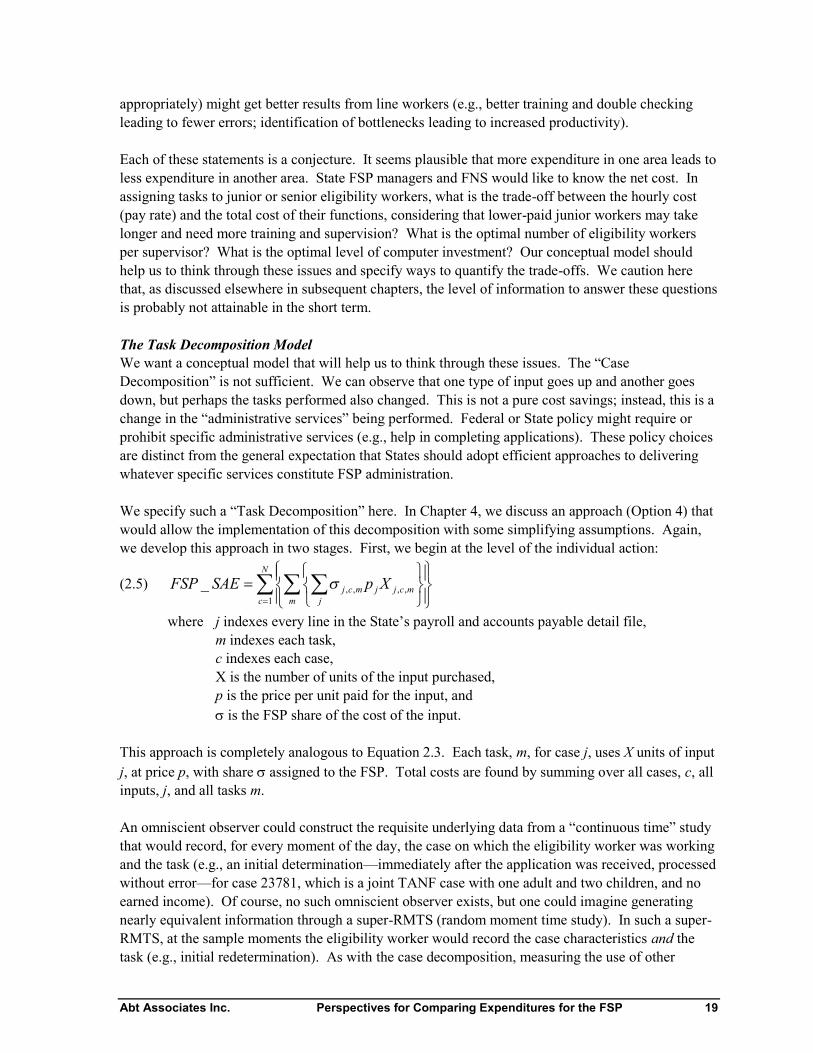
Abt Associates Inc. Perspectives for Comparing Expenditures for the FSP 19
appropriately) might get better results from line workers (e.g., better training and double checkingleading to fewer errors; identification of bottlenecks leading to increased productivity).
Each of these statements is a conjecture. It seems plausible that more expenditure in one area leads toless expenditure in another area. State FSP managers and FNS would like to know the net cost. Inassigning tasks to junior or senior eligibility workers, what is the trade-off between the hourly cost(pay rate) and the total cost of their functions, considering that lower-paid junior workers may takelonger and need more training and supervision? What is the optimal number of eligibility workersper supervisor? What is the optimal level of computer investment? Our conceptual model shouldhelp us to think through these issues and specify ways to quantify the trade-offs. We caution herethat, as discussed elsewhere in subsequent chapters, the level of information to answer these questionsis probably not attainable in the short term.
The Task Decomposition ModelWe want a conceptual model that will help us to think through these issues. The “CaseDecomposition” is not sufficient. We can observe that one type of input goes up and another goesdown, but perhaps the tasks performed also changed. This is not a pure cost savings; instead, this is achange in the “administrative services” being performed. Federal or State policy might require orprohibit specific administrative services (e.g., help in completing applications). These policy choicesare distinct from the general expectation that States should adopt efficient approaches to deliveringwhatever specific services constitute FSP administration.
We specify such a “Task Decomposition” here. In Chapter 4, we discuss an approach (Option 4) thatwould allow the implementation of this decomposition with some simplifying assumptions. Again,we develop this approach in two stages. First, we begin at the level of the individual action:
(2.5)
N
c m jmcjjmcj XpSAEFSP
1,,,,_
where j indexes every line in the State’s payroll and accounts payable detail file,m indexes each task,c indexes each case,X is the number of units of the input purchased,p is the price per unit paid for the input, and is the FSP share of the cost of the input.
This approach is completely analogous to Equation 2.3. Each task, m, for case j, uses X units of inputj, at price p, with share assigned to the FSP. Total costs are found by summing over all cases, c, allinputs, j, and all tasks m.
An omniscient observer could construct the requisite underlying data from a “continuous time” studythat would record, for every moment of the day, the case on which the eligibility worker was workingand the task (e.g., an initial determination—immediately after the application was received, processedwithout error—for case 23781, which is a joint TANF case with one adult and two children, and noearned income). Of course, no such omniscient observer exists, but one could imagine generatingnearly equivalent information through a super-RMTS (random moment time study). In such a super-RMTS, at the sample moments the eligibility worker would record the case characteristics and thetask (e.g., initial redetermination). As with the case decomposition, measuring the use of other
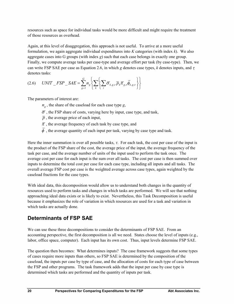
20 Perspectives for Comparing Expenditures for the FSP Abt Associates Inc.
resources such as space for individual tasks would be more difficult and might require the treatmentof those resources as overhead.
Again, at this level of disaggregation, this approach is not useful. To arrive at a more usefulformulation, we again aggregate individual expenditures into K categories (with index k). We alsoaggregate cases into G groups (with index g) such that each case belongs in exactly one group.Finally, we compute average tasks per case-type and average effort per task (by case-type). Then, wecan write FSP SAE per case as Equation 2.6, in which g denotes case types, k denotes inputs, and denotes tasks:
(2.6)
G
g kgkgkgkg pnSAEFSPUNIT
1,,,,,__
The parameters of interest are:
gn , the share of the caseload for each case type g,
, the FSP share of costs, varying here by input, case type, and task,p , the average price of each input, , the average frequency of each task by case type, and
, the average quantity of each input per task, varying by case type and task.
Here the inner summation is over all possible tasks, . For each task, the cost per case of the input isthe product of the FSP share of the cost, the average price of the input, the average frequency of thetask per case, and the average number of units of the input used to perform the task once. Theaverage cost per case for each input is the sum over all tasks. The cost per case is then summed overinputs to determine the total cost per case for each case type, including all inputs and all tasks. Theoverall average FSP cost per case is the weighted average across case types, again weighted by thecaseload fractions for the case types.
With ideal data, this decomposition would allow us to understand both changes in the quantity ofresources used to perform tasks and changes in which tasks are performed. We will see that nothingapproaching ideal data exists or is likely to exist. Nevertheless, this Task Decomposition is usefulbecause it emphasizes the role of variation in which resources are used for a task and variation inwhich tasks are actually done.
Determinants of FSP SAE
We can use these three decompositions to consider the determinants of FSP SAE. From anaccounting perspective, the first decomposition is all we need. States choose the level of inputs (e.g.,labor, office space, computer). Each input has its own cost. Thus, input levels determine FSP SAE.
The question then becomes: What determines inputs? The case framework suggests that some typesof cases require more inputs than others, so FSP SAE is determined by the composition of thecaseload, the inputs per case by type of case, and the allocation of costs for each type of case betweenthe FSP and other programs. The task framework adds that the input per case by case type isdetermined which tasks are performed and the quantity of inputs per task.
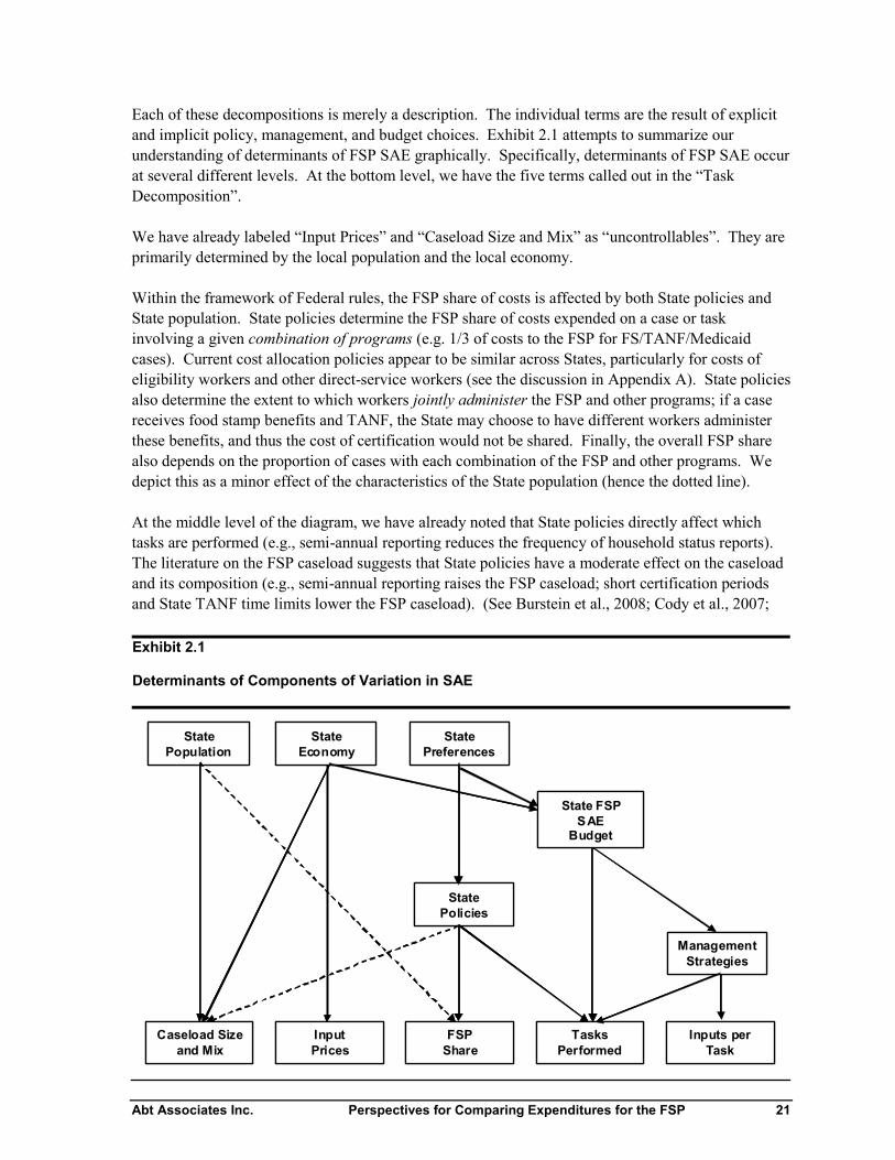
Abt Associates Inc. Perspectives for Comparing Expenditures for the FSP 21
Each of these decompositions is merely a description. The individual terms are the result of explicitand implicit policy, management, and budget choices. Exhibit 2.1 attempts to summarize ourunderstanding of determinants of FSP SAE graphically. Specifically, determinants of FSP SAE occurat several different levels. At the bottom level, we have the five terms called out in the “TaskDecomposition”.
We have already labeled “Input Prices” and “Caseload Size and Mix” as “uncontrollables”. They areprimarily determined by the local population and the local economy.
Within the framework of Federal rules, the FSP share of costs is affected by both State policies andState population. State policies determine the FSP share of costs expended on a case or taskinvolving a given combination of programs (e.g. 1/3 of costs to the FSP for FS/TANF/Medicaidcases). Current cost allocation policies appear to be similar across States, particularly for costs ofeligibility workers and other direct-service workers (see the discussion in Appendix A). State policiesalso determine the extent to which workers jointly administer the FSP and other programs; if a casereceives food stamp benefits and TANF, the State may choose to have different workers administerthese benefits, and thus the cost of certification would not be shared. Finally, the overall FSP sharealso depends on the proportion of cases with each combination of the FSP and other programs. Wedepict this as a minor effect of the characteristics of the State population (hence the dotted line).
At the middle level of the diagram, we have already noted that State policies directly affect whichtasks are performed (e.g., semi-annual reporting reduces the frequency of household status reports).The literature on the FSP caseload suggests that State policies have a moderate effect on the caseloadand its composition (e.g., semi-annual reporting raises the FSP caseload; short certification periodsand State TANF time limits lower the FSP caseload). (See Burstein et al., 2008; Cody et al., 2007;
Exhibit 2.1
Determinants of Components of Variation in SAE
StatePopulation
StateEconomy
StatePreferences
StatePolicies
State FSPSAE
Budget
ManagementStrategies
Inputs perTask
TasksPerformed
FSPShare
InputPrices
Caseload Sizeand Mix
StatePopulation
StateEconomy
StatePreferences
StatePolicies
State FSPSAE
Budget
ManagementStrategies
Inputs perTask
TasksPerformed
FSPShare
InputPrices
Caseload Sizeand Mix
22 Perspectives for Comparing Expenditures for the FSP Abt Associates Inc.
Ratcliffe et al., 2008.) We consider this effect to be minor and therefore draw it with a dotted line.Management strategies also affect the resources used for each task; these include agencyorganization, design of processes, and standards for how tasks are performed. Recent innovations inmanagement include Web-based applications, use of community partners to provide sites forsubmitting applications, and call centers to process case changes (GAO, 2007).
Ultimately, each of these choices is determined by a State’s preferences as expressed in the politicalenvironment. State preferences directly determine State policies. States allocate their own funds forFSP administration; these are matched by Federal funds. The FSP SAE budget is determined by theinterplay of State fiscal capacity, other demands on the State government, the perceived value ofexpenditures on the State’s poorer population, and the level of performance that the State seeks toattain. Based on their budgets, State FSP administrators choose input levels and managementstrategies.16 These choices, together with the composition and volatility of the caseload, determinecertification accuracy and service levels. Lower budgets yield lower input levels, less accuracy, andless service; e.g., less outreach, longer wait times, less help in filling out applications.
While not shown in the model, Federal policies also affect which tasks are performed and how theyare performed. Changes in these policies may affect variation in SAE over time and the relativedifficulty of tasks for different case types. For example, the restrictions on eligibility for noncitizensenacted in PRWORA added to the workload for certifying households with noncitizen members,while the later relaxation of these restrictions had the opposite effect. We focus on State policies,since they vary across States, and our primary focus is on explaining interstate variation in SAE.
In the conceptual framework, the levels interact. States may choose policies that reduce the numberof tasks that must be performed. However, a task-saving policy change (such as simplified reporting)will not directly affect total FSP SAE unless the staffing level is cut at the same time. Thus, at leastin the short run, what we observe is not the full potential savings of the change, but the savingsrealized by the agency when it implements the change. Ideally, the State would monitor and adjuststaffing levels in response to opportunities for savings and demand for increased staffing (e.g., raisingstaffing levels as error rates rise or as time to process applications exceeds the regulatoryrequirement). In reality, such adjustments are difficult to make in the short run; State managersinterviewed for this study indicated that their staffing levels tend to remain fixed within a budgetperiod (either one or two years, depending on State practices). Thus, changes in staffing will tend tooccur with long lags—if at all.
16 It may be argued that State FSP SAE costs affect policy choices: a State with high costs might changepolicies to reduce effort, e.g., lengthening certification periods. If policy choices were endogenous, thenestimates of the impacts of the policies on costs might be biased. However, we do not believe it isnecessary or appropriate to view policy choices as directly affected by short-term variations in State budgetconditions. We do not observe policies fluctuating in response to changes in costs. Instead, States appearto retain effort-saving policies, such as expanded categorical eligibility, once these policies are adopted.Therefore, we instead focus on the role of State preferences in determining policies. These preferencesmay include a general desire to reduce spending, whether costs are high or not. We frame the choice ofmanagement strategies as driven by the State budget, not actual costs, because the budget reflects otherconsiderations besides past costs. We acknowledge that budgets affect the implementation of policiesthrough tasks actually performed. Ideally, the possibility that policies are endogenous would be consideredin models of SAE. In the absence of an experimental design, addressing this possibility would require amethod such as instrumental variables (IV). The challenges of this approach are discussed in ChapterThree.
Abt Associates Inc. Perspectives for Comparing Expenditures for the FSP 23
The other direction of change is also crucial. Consider what happens when caseloads rise within aState’s budget cycle. Without a change, FSP SAE per case will fall. The State may respond byadopting policies that reduce the number of tasks, in order to spread the existing staff over morecases. In extreme cases, there may be a supplementary budget—to return FSP SAE per case to someacceptable level. Given that caseloads often rise because the economy got worse, the State mightinstead cut total FSP SAE (and therefore cut per-case FSP SAE even more).
Practically speaking, State FSP organizations continue to operate at almost any funding level—andwe observe widely varying funding levels across States and through time. It is crucial to ask, whathappens? How do high FSP SAE States differ from low FSP SAE States; assuming—as seemsplausible—that the difference is not merely in uncontrollables (input prices and case mix). It seemslikely that somewhere there is some difference in tasks actually performed. That difference in tasks ispartially observable. We can observe events that are recorded in case files: initial certifications,interim changes, periodic reports, recertifications, and closures. We can observe the time to processinitial applications and certification error rates for initial certifications, recertifications, and ongoingcases (case maintenance). However, it seems likely that much of the difference in tasks is notobserved. We do not observe specific outreach activities, answering phone calls, help onapplications, reviewing matches with third-party data sources, or screening of clients who do notapply. We do not observe all of the delays and inconveniences that applicants and participantsexperience as eligibility worker caseloads rise.
In as much as a future study of SAE finds differences in controllables, it seems likely that some ofthat difference is in task frequency and quality. Some of these differences can be observed, whileothers cannot. Only by collecting data and conducting analysis can we determine how much of thedifference can be explained with the tasks that can be observed. The data collection will also provideinsight in the kinds of tasks that are not observed, or the level of detail that is missing. This insightwill help interpret the significance of the unexplained variation; for example, the unobserved tasksmay be “nice but not essential”, and the policy implication would be that costs could be reduced byshifting high-cost States to the pattern of tasks performed by the low-cost States. We are not assuredin advance, however, that the amount of explained variation will be sufficient to lead to such clearinterpretation.
Implications of the Model
We conclude this chapter with a brief discussion of its implications for the study of FSP SAE. Weargued in the first chapter that any study of FSP SAE should have two complementary goals. First,such a study should try to decompose observed variation in FSP SAE. Second, such a study shouldtry to understand the influence of certain specific factors—particularly policies—on FSP SAE.
Decomposing Observed Variation
With respect to the first goal—decomposing observed variation, we have argued that Equation 2.6provides an ideal—but unattainable—goal for the decomposition. Ideally, we would like tounderstand the separate contributions of variation in (a) case mix, (b) input prices, (c) tasksperformed, and (d) resources per task. Ideally, we would perform such a decomposition using a formof a “shift-share” analysis. Specifically, if we knew all of the terms in Equation 2.6, we could ask:How much variation would be left if every State faced the same case mix or input prices or tasks
24 Perspectives for Comparing Expenditures for the FSP Abt Associates Inc.
performed or resources per task. The resulting decrease in variation in FSP SAE would give us ameasure of the importance of each source of variation in explaining overall variation in FSP SAE.
Furthermore, we argued in Chapter 1 that understanding the importance of each source of variationwould be insightful for determining whether observed variation in FSP SAE represents a potential forcost savings. In as much as FSP SAE varies because of uncontrollables—input prices and case mix—there seems to be little scope for cost savings. On the other hand, in as much as FSP SAE variesbecause of tasks performed or resources per task, there is more scope for cost savings. States couldbe encouraged (or required) to limit the tasks they perform or to adopt more efficient methods forperforming tasks.
Much of the balance of this report is devoted to specifying feasible approaches to such adecomposition of overall variation in SAE. We will argue that with plausible (though notunassailable) assumptions and data obtainable at moderate cost, it is possible to identify the separateeffects of the uncontrollables: input prices and case mix. Progress towards decomposingcontrollables into effects on tasks performed and resources per task appears to be more difficult butfeasible. We suggest some partial approaches.
Understanding the Role of Specific Factors
With respect to the second goal—understanding the role of specific factors, we have argued thatEquation 2.6 provides an ideal—but unattainable—goal for the decomposition. We will argue in thenext chapter that two complementary approaches are possible. One approach is “reduced form”. Itsimply specifies a reduced form regression of total FSP SAE on the factors of interest (e.g., inputprices, case mix, specific policies, local political and budgetary conditions).
The alternative is a “structural” approach that attempts to specify an empirical model in a system ofequations that simplifies but approximates the conceptual model developed here. One such path is toseek to measure and model the cost components identified in the three decompositions of SAE.Instead of modeling aggregate FSP SAE, we might model the costs of individual inputs charged tothe FSP—labor, rent, overhead, other. In Chapter 3, we will argue that that the structure of State datais likely to preclude such an “accounting decomposition” approach, but one key input in particularcould be measured and modeled: eligibility worker time. Similarly, one might model total costsattributed to a case type or to a task. It appears impossible to obtain a direct measure of total costs atthe case or task level, but partial approaches appear possible.
Second, we might try to proxy for some of the terms in Equation 2.6. Even if we cannot directlymeasure cost by case-type or cost by task, we argue in Chapter 3 that it might be possible to constructproxies for the effect of variation in case-type or tasks performed. To be exactly true, thoseapproaches require heroic and clearly incorrect assumptions. However, modeling aggregate datausing reduced form approaches also requires heroic (but usually implicit) assumptions. We suggestthat such proxies are likely lead to insightful analyses. We develop these ideas in the next chapter.We also note that pursuing the structural approach does not preclude the reduced-form approach;indeed the most robust study would use both.
Beyond this reduced-form/structural distinction, our discussion of the determinants of FSP SAEsuggests some caution in interpreting estimates of the effects of the determinants of FSP SAE. Statesdirectly control FSP SAE through their budget process. One therefore needs to think carefully about
Abt Associates Inc. Perspectives for Comparing Expenditures for the FSP 25
how, for example, policy changes affect FSP SAE. Suppose a State adopts a task-saving policy (e.g.,semi-annual reporting). That change might have no direct effect on FSP SAE. The eligibilityworkers are still on the payroll. They might spend the same time to do fewer tasks—i.e., theirproductivity would drop, but this change might be a shift to a more sustainable level with lessturnover and burnout. Alternatively, they might do more of other tasks (e.g., more time helpingapplicants to complete their application, more accurate initial certifications, more timely processingof initial applications). On the other hand, while the total payroll remains the same, FSP SAE coulddecrease if workers might spend less time on the FSP and more time on other programs. Thechallenge of sorting through these possible effects is that our ability to conceptualize them exceedsour potential to measure them. How we cope with this challenge is a theme of the remaining chaptersof this report.

26 Perspectives for Comparing Expenditures for the FSP Abt Associates Inc.
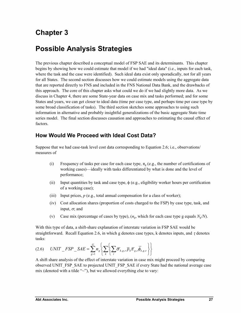
Abt Associates Inc. Possible Analysis Strategies 27
Chapter 3
Possible Analysis Strategies
The previous chapter described a conceptual model of FSP SAE and its determinants. This chapterbegins by showing how we could estimate that model if we had "ideal data" (i.e., inputs for each task,where the task and the case were identified). Such ideal data exist only sporadically, not for all yearsfor all States. The second section discusses how we could estimate models using the aggregate datathat are reported directly to FNS and included in the FNS National Data Bank, and the drawbacks ofthis approach. The core of this chapter asks what could we do if we had slightly more data. As wediscuss in Chapter 4, there are some State-year data on case mix and tasks performed; and for someStates and years, we can get closer to ideal data (time per case type, and perhaps time per case type bysome broad classification of tasks). The third section sketches some approaches to using suchinformation in alternative and probably insightful generalizations of the basic aggregate State timeseries model. The final section discusses causation and approaches to estimating the causal effect offactors.
How Would We Proceed with Ideal Cost Data?
Suppose that we had case-task level cost data corresponding to Equation 2.6; i.e., observations/measures of
(i) Frequency of tasks per case for each case type, πg (e.g., the number of certifications ofworking cases)—ideally with tasks differentiated by what is done and the level ofperformance;
(ii) Input quantities by task and case type, (e.g., eligibility worker hours per certificationof a working case);
(iii) Input prices, p (e.g., total annual compensation for a class of worker);
(iv) Cost allocation shares (proportion of costs charged to the FSP) by case type, task, andinput, ; and
(v) Case mix (percentage of cases by type), (ng, which for each case type g equals Ng/N).
With this type of data, a shift-share explanation of interstate variation in FSP SAE would bestraightforward. Recall Equation 2.6, in which g denotes case types, k denotes inputs, and denotes tasks:
(2.6)
G
g kgkgkgkg pnSAEFSPUNIT
1,,,,,__
A shift share analysis of the effect of interstate variation in case mix might proceed by comparingobserved UNIT_FSP_SAE to projected UNIT_FSP_SAE if every State had the national average casemix (denoted with a tilde “~”), but we allowed everything else to vary:
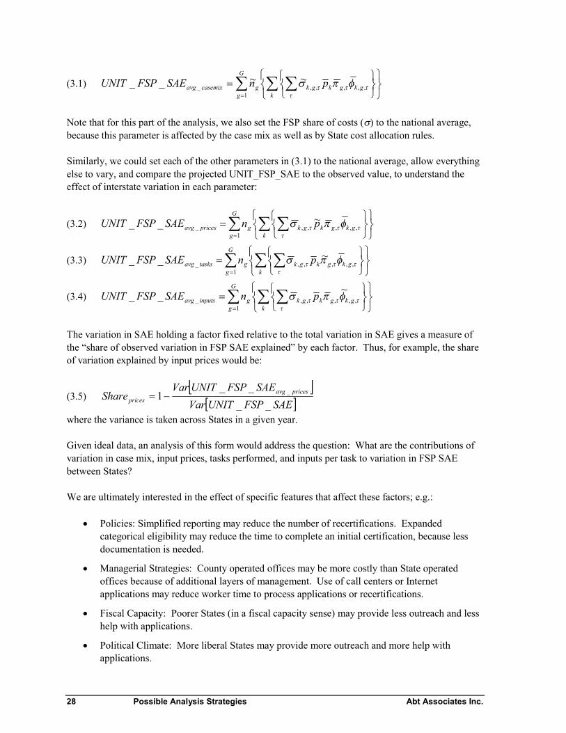
28 Possible Analysis Strategies Abt Associates Inc.
(3.1)
G
g kgkgkgkgcasemixavg pnSAEFSPUNIT
1,,,,,_
~~__
Note that for this part of the analysis, we also set the FSP share of costs () to the national average,because this parameter is affected by the case mix as well as by State cost allocation rules.
Similarly, we could set each of the other parameters in (3.1) to the national average, allow everythingelse to vary, and compare the projected UNIT_FSP_SAE to the observed value, to understand theeffect of interstate variation in each parameter:
(3.2)
G
g kgkgkgkgpricesavg pnSAEFSPUNIT
1,,,,,_
~__
(3.3)
G
g kgkgkgkgtasksavg pnSAEFSPUNIT
1,,,,,_
~__
(3.4)
G
g kgkgkgkginputsavg pnSAEFSPUNIT
1,,,,,_
~__
The variation in SAE holding a factor fixed relative to the total variation in SAE gives a measure ofthe “share of observed variation in FSP SAE explained” by each factor. Thus, for example, the shareof variation explained by input prices would be:
(3.5)
SAEFSPUNITVar
SAEFSPUNITVarShare pricesavg
prices __
__1 _
where the variance is taken across States in a given year.
Given ideal data, an analysis of this form would address the question: What are the contributions ofvariation in case mix, input prices, tasks performed, and inputs per task to variation in FSP SAEbetween States?
We are ultimately interested in the effect of specific features that affect these factors; e.g.:
Policies: Simplified reporting may reduce the number of recertifications. Expandedcategorical eligibility may reduce the time to complete an initial certification, because lessdocumentation is needed.
Managerial Strategies: County operated offices may be more costly than State operatedoffices because of additional layers of management. Use of call centers or Internetapplications may reduce worker time to process applications or recertifications.
Fiscal Capacity: Poorer States (in a fiscal capacity sense) may provide less outreach and lesshelp with applications.
Political Climate: More liberal States may provide more outreach and more help withapplications.
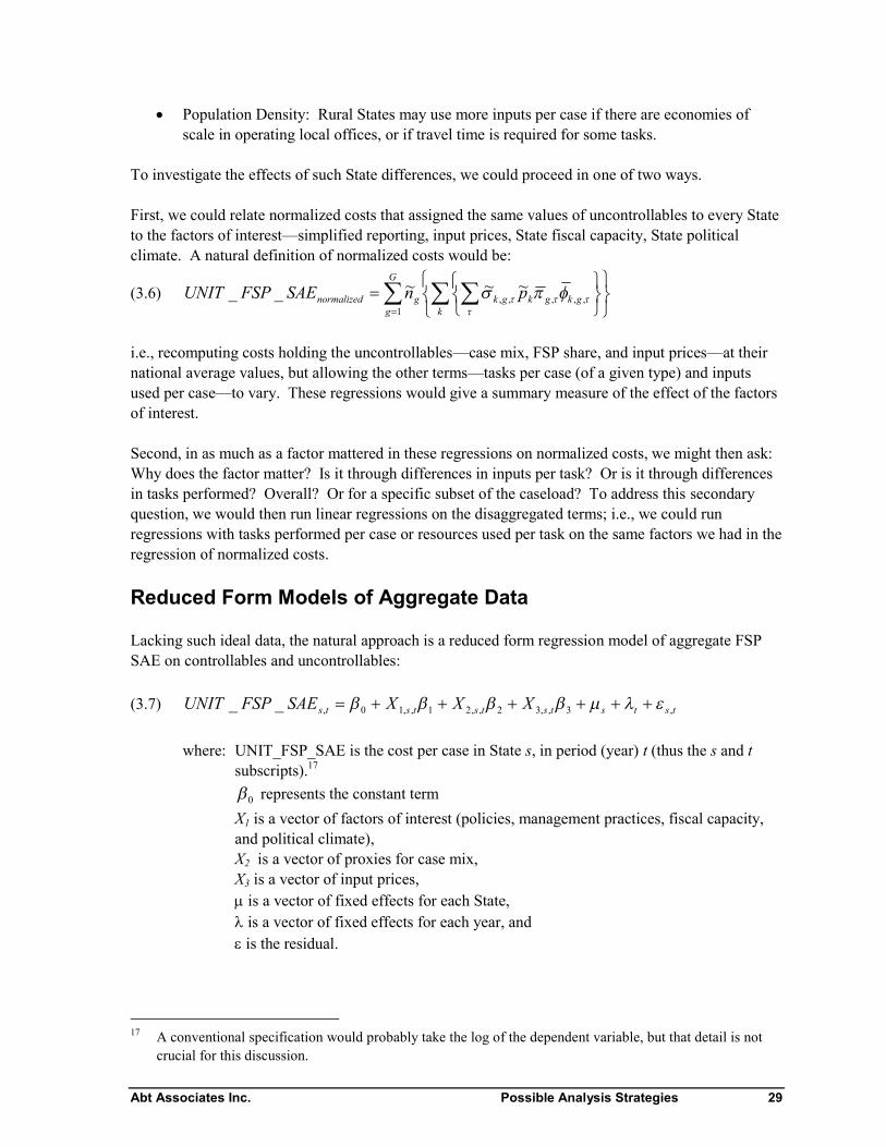
Abt Associates Inc. Possible Analysis Strategies 29
Population Density: Rural States may use more inputs per case if there are economies ofscale in operating local offices, or if travel time is required for some tasks.
To investigate the effects of such State differences, we could proceed in one of two ways.
First, we could relate normalized costs that assigned the same values of uncontrollables to every Stateto the factors of interest—simplified reporting, input prices, State fiscal capacity, State politicalclimate. A natural definition of normalized costs would be:
(3.6)
G
g kgkgkgkgnormalized pnSAEFSPUNIT
1,,,,,
~~~__
i.e., recomputing costs holding the uncontrollables—case mix, FSP share, and input prices—at theirnational average values, but allowing the other terms—tasks per case (of a given type) and inputsused per case—to vary. These regressions would give a summary measure of the effect of the factorsof interest.
Second, in as much as a factor mattered in these regressions on normalized costs, we might then ask:Why does the factor matter? Is it through differences in inputs per task? Or is it through differencesin tasks performed? Overall? Or for a specific subset of the caseload? To address this secondaryquestion, we would then run linear regressions on the disaggregated terms; i.e., we could runregressions with tasks performed per case or resources used per task on the same factors we had in theregression of normalized costs.
Reduced Form Models of Aggregate Data
Lacking such ideal data, the natural approach is a reduced form regression model of aggregate FSPSAE on controllables and uncontrollables:
(3.7) tstststststs XXXSAEFSPUNIT ,3,,32,,21,,10,__
where: UNIT_FSP_SAE is the cost per case in State s, in period (year) t (thus the s and tsubscripts).17
0 represents the constant term
X1 is a vector of factors of interest (policies, management practices, fiscal capacity,and political climate),X2 is a vector of proxies for case mix,X3 is a vector of input prices, is a vector of fixed effects for each State,is a vector of fixed effects for each year, andis the residual.
17 A conventional specification would probably take the log of the dependent variable, but that detail is notcrucial for this discussion.
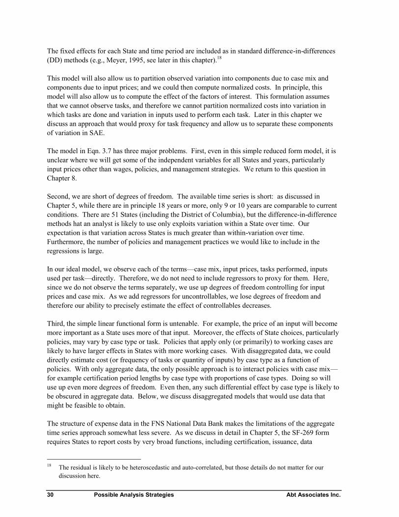
30 Possible Analysis Strategies Abt Associates Inc.
The fixed effects for each State and time period are included as in standard difference-in-differences(DD) methods (e.g., Meyer, 1995, see later in this chapter).18
This model will also allow us to partition observed variation into components due to case mix andcomponents due to input prices; and we could then compute normalized costs. In principle, thismodel will also allow us to compute the effect of the factors of interest. This formulation assumesthat we cannot observe tasks, and therefore we cannot partition normalized costs into variation inwhich tasks are done and variation in inputs used to perform each task. Later in this chapter wediscuss an approach that would proxy for task frequency and allow us to separate these componentsof variation in SAE.
The model in Eqn. 3.7 has three major problems. First, even in this simple reduced form model, it isunclear where we will get some of the independent variables for all States and years, particularlyinput prices other than wages, policies, and management strategies. We return to this question inChapter 8.
Second, we are short of degrees of freedom. The available time series is short: as discussed inChapter 5, while there are in principle 18 years or more, only 9 or 10 years are comparable to currentconditions. There are 51 States (including the District of Columbia), but the difference-in-differencemethods hat an analyst is likely to use only exploits variation within a State over time. Ourexpectation is that variation across States is much greater than within-variation over time.Furthermore, the number of policies and management practices we would like to include in theregressions is large.
In our ideal model, we observe each of the terms—case mix, input prices, tasks performed, inputsused per task—directly. Therefore, we do not need to include regressors to proxy for them. Here,since we do not observe the terms separately, we use up degrees of freedom controlling for inputprices and case mix. As we add regressors for uncontrollables, we lose degrees of freedom andtherefore our ability to precisely estimate the effect of controllables decreases.
Third, the simple linear functional form is untenable. For example, the price of an input will becomemore important as a State uses more of that input. Moreover, the effects of State choices, particularlypolicies, may vary by case type or task. Policies that apply only (or primarily) to working cases arelikely to have larger effects in States with more working cases. With disaggregated data, we coulddirectly estimate cost (or frequency of tasks or quantity of inputs) by case type as a function ofpolicies. With only aggregate data, the only possible approach is to interact policies with case mix—for example certification period lengths by case type with proportions of case types. Doing so willuse up even more degrees of freedom. Even then, any such differential effect by case type is likely tobe obscured in aggregate data. Below, we discuss disaggregated models that would use data thatmight be feasible to obtain.
The structure of expense data in the FNS National Data Bank makes the limitations of the aggregatetime series approach somewhat less severe. As we discuss in detail in Chapter 5, the SF-269 formrequires States to report costs by very broad functions, including certification, issuance, data
18 The residual is likely to be heteroscedastic and auto-correlated, but those details do not matter for ourdiscussion here.
Abt Associates Inc. Possible Analysis Strategies 31
processing, fraud control, employment and training, and nutrition education. To the extent that theseindividual functions are of interest and consistently defined, we could run the aggregate regressionsseparately for each task. As stated in Chapter 1, we have assumed that the primary interest is incertification costs. The appropriate set of regressors for a given function will be smaller in numberthan the regressors for a model of total SAE. Nevertheless, a complete model of certification costssimilar to Equation 3.7 would entail a large—potentially overwhelming—array of variables. Wereturn to the feasibility of this approach in Chapter 4.
Alternative Disaggregated Models
The modeling question is then: Is there some way to use data that are available or obtainable (atreasonable cost) to address these problems with the aggregate time series regressions and thereby toget closer to the ideal task decomposition model? This section considers four such approaches. Thefirst approach exploits separate estimates of cost by type of input. The second approach explains howto exploit information on costs by case type. The third approach suggests a way to use more limitedinformation on costs by case type. The fourth approach offers a way to approximate costs by task.Thus, in terms of the levels of disaggregation in Chapter 2, the first approach disaggregates costs atthe input level, the second and third at the case level, and the fourth at the task level.
Simplified Models to Decompose Aggregate Cost
The ideal model assumed cost data for each type of input. Even if that information is not available, itseems plausible that we might be able to get data on variations in the most important cost component,compensation for eligibility workers, because of the information States must gather to allocate localoffice costs among program. (The nature of this information is discussed in Chapter 5.) Thissuggests a model with two inputs: eligibility workers and “everything else”.19 All factors other thaneligibility worker labor could be treated as a generalized “overhead”, proportional to eligibilityworker cost. This approach is similar in spirit to cost allocation rules, which allow States to allocateall local agency costs—including eligibility workers, support staff, supervisors, and non-labor costs—and some State agency costs by program in proportion to eligibility worker time or cost.20 Our modelis then:
(3.8) tstststs wpSAEFSPUNIT ,,1
,,__
where p1 is the hourly eligibility worker wage, w is the ratio of FSP eligibility worker time to cases (ameasure of staffing intensity equal the inverse of FSP eligibility worker caseload), and α is theoverhead markup factor (i.e., the ratio of overhead costs to total eligibility worker pay). The FSPeligibility worker time per case (w) incorporates the FSP share factor for this input ( ). As discussed
19 As discussed later in the report, the definition of an eligibility worker is subject to variation. For thisdiscussion, an eligibility worker is one who obtains eligibility information from clients or makesdeterminations of eligibility and benefits based on information collected by others.
20 One can, of course, identify specific costs for which this assumption may not be appropriate: for example,the cost of application forms would be a function of the number of cases, not eligibility worker time or cost.Analysis of the composition of overhead, as discussed in the text, would indicate whether the principalcomponents of overhead are reasonably related to eligibility worker hours.
32 Possible Analysis Strategies Abt Associates Inc.
below, this time could be modeled as a function of policies (including cost allocation rules) and casemix.
This model would greatly oversimplify SAE if it were applied to the total cost for all FSP functions.It is particularly simplistic to treat as “overhead” client services that are not performed by eligibilityworkers, including issuance, nutrition education, outreach, and employment and training. Instead,this approach is more suited to analysis focused on a specific function, particularly certification andrelated costs (which might include data processing). The issue of the definition of “certification” foranalysis of SAE is discussed in Chapter 5.
This “eligibility worker plus overhead” model is potentially implementable with available State-leveldata. In principle, we could collect information from State cost allocation records and payrolls on theeligibility worker cost charged to the FSP and the average compensation of these workers. We thencould use these data to compute the number of eligibility worker hours per case charged to the FSP(or this information might be available directly). We know SAE per case, so we can compute thegeneralized overhead rate, by simple division. If we had these data, we could then use Equation 3.7 to begin to understand the sources of variation in SAE across States.
From a model of this form, one could address the questions of interest, using the components ofvariation in cost. First, we could compute the proportion of variation in SAE attributable to each ofthe three components of the model: eligibility worker wages, eligibility worker time per case, and“everything else”. Second, we could explore the determinants of these components in separatemodels. For example, we could analyze the relationship of eligibility worker pay to one or morespecific benchmark occupations in the private sector, such as claims processors for insurancecompanies, or to the broad occupational group that includes eligibility workers. A State’s relative paylevel for the benchmark occupation(s) (i.e., State average divided by national average) would predictits relative pay for eligibility workers if eligibility worker pay were determined by the same segmentof the labor market as the benchmark occupations.21 Such benchmarks could be used to compute aquality-adjusted measure of eligibility worker time (with the assumption that eligibility workers paidmore than the State market rate would require fewer hours per case).22 Policy variables and case mixwould enter in the model of eligibility worker time per case. Management and fiscal variables wouldenter into both the eligibility worker time per case and overhead. For example, the eligibility workermodel might include whether workers specialize in the FSP or serve multiple programs. State versuscounty administration would be a variable in the model of overhead.
As an additional step in the analysis, it may be feasible to collect additional data allowing thedecomposition of “overhead” costs between other local staff, local nonlabor costs (such as rent), and
21 This approach does not require the assumption that the pay for the benchmark occupation would be equal tothe eligibility worker pay set on a purely market basis, only that the relative pay differential would be thesame.
22 The model of eligibility worker pay versus the benchmark could be a simple univariate relationship, orother factors such as economic trends and union strength could be considered. The latter approach wouldprovide more insight into the reasons for eligibility worker pay differentials (e.g., workers accept lower payfor public jobs when private employment is more volatile). In computing the quality-adjusted measure ofeligibility worker time, there would be a question of whether to assume that higher pay in the presence ofunions would result in better workers, or whether this reflects market power on the part of the existing workforce.
Abt Associates Inc. Possible Analysis Strategies 33
State costs. We could then determine the contribution of each element to cost variation andseparately model differences in (a) ratio of other local staff costs (or time) to eligibility workers, (b)input prices of local nonlabor costs, such as rent, (c) ratio of normalized local nonlabor costs (usingaverage input prices) to total local staff time, and (d) ratio of State costs to local costs.
Note, however, that this approach continues to deal with caseload heterogeneity via regressors thatare part of models with potentially numerous policy and management variables. Below we suggestways to avoid this limitation by further disaggregating SAE, either by case type or by task.
Separate Models of Costs by Case Type
The preceding approach to disaggregating costs by modeling aggregate data (3.6) ignores the effect ofdifferences in cost by case type, which might be possible to measure. Most States use random-moment time studies (RMTS) as the basis for allocating eligibility worker costs across programs.23
These studies collect data on the type of case being served by randomly selected workers at randomlyselected moments. It may be possible to attribute the actions in these random moment time study datato specific types of food stamp cases, through the extant data or through matching to case records(using the case number, which is sometimes collected in these data). If we had data on workermoments by FSP case type, we could estimate the proportion of costs by case type, using thedistribution of eligibility worker time to apportion total costs (implicitly incorporating other costs asoverhead). Then we could run separate aggregate regressions of total cost or eligibility worker timeper case for each case type. Given this stratification, we would not need to include proxies for casemix. It seems plausible that the structure of costs would be more similar across States within a casetype than for aggregate costs (even with case mix proxies).24
An Index Approach to Caseload Heterogeneity
Alternatively, if such RMTS data matched to case characteristics were available for some States andyears, we could use them to estimate the models of the previous sub-section. Such data are clearlynot available or even recoverable for all States back very many years (see the discussion below inChapter 5). Given that reality and given that difference-of-difference models benefit from long time-series and many States, a natural question becomes: Can we devise some way to use insights about“case difficulty” from States and years where we have the richer data in our analysis of States andyears for which we do not have the richer data (i.e., the full 17 plus year time series of State data).
Our approach follows from the hypothesis that some cases are “harder” (more difficult, more resourceintensive) than others. We would expect that working cases are harder; earnings and therefore thecorrect benefit change frequently. Cases with more people and more adults require more initialverification and are likely to change membership more often. Joint TANF cases have their FSP SAEcosts split with TANF, so the FSP SAE attributed cost is smaller.
23 For a description of random-moment time studies, see Appendix B.24 One might try to model the costs of labor, data processing, and other inputs in separate models. This
approach would assume that inputs are independent of each other, an assumption that is questionable, aspreviously discussed in the section on aggregate modeling. Moreover, the approaches already discussedseparate eligibility worker labor—which we understand to be the largest input—from other costs.
34 Possible Analysis Strategies Abt Associates Inc.
For example cases with earnings might, on average, require 2.3 times as many eligibility workerhours per month as cases without earnings. One could then assume that this ratio is constant acrossall States for the time period under study.25 A benchmark case type would be defined (e.g., twochildren and a nonworking, nonelderly adult), and this case type would have a difficulty factor of 1.We then define a measure of “intensity” that represents the actual eligibility worker time per case(across all case types) adjusted for the average difficulty of the caseload. The intensity measurevaries by State and over time. A State with a 5 percent greater intensity measure than the averageState would spend 5 percent more eligibility worker time per case if it had the average case mix. AState with higher “intensity” is one where FSP administration is more “eligibility worker intensive”.Thus, this approach also offers a way to relate States’ use of resources to their performance whenperformance is not an element of the definition of a task. Whether a State with higher intensity thanthe average State is less productive depends on the State’s error rate and other measures ofeffectiveness, after controlling for other factors that may affect their use of resources.
It seems plausible that such variation in difficult exists and that it is roughly similar across States andtime.26 If so, then the following strategy seems promising:
1. Estimate the relative difficulty in States where we have RMTS data linked to case records;i.e., estimate average (cost weighted) eligibility worker hours by case type.
2. Normalize by some case type (e.g., two adults and two children).
3. Then use those factors and aggregate data on case mix to extrapolate to the other States andyears.
Formally, we might proceed as follows. We begin with the “eligibility worker and overhead model”(i.e., Equation 3.8), which defines SAE per case as the product of the “overhead” ratio (), theeligibility worker pay rate (p), and the eligibility worker time per case (w). We recognize that theaverage eligibility worker hours per case will vary by case type. Therefore, we modify 3.8 to expresseligibility worker time per case as the weighted average of eligibility worker hours per case for eachcase type, where the weights are the shares of each case type in the caseload:
(3.9)
g
tsg
tsg
tststs npSAEFSPUNIT ,,,,,__
where: ng is the fraction of the caseload of type g, varying by State and time,g is a “difficulty factor” that varies by case type (g) but not by State, ands,t is a State-specific “intensity factor” (worker hours per standard case) that varies by State(s) and over time (t) but not by case type.
25 A variant of this approach would be to assign to each State the ratio from the most similar State(s) forwhich data were obtained, if there were a single dimension that was considered sufficiently important.
26 It seems unlikely that the relative difficulty of cases is identical across States and time. For example somepolicies differentially affect certain case types. States may use automation or specialization to reduce thedifficulty of particular kinds of cases (e.g., creating specialized units of bilingual workers to serve clientswith limited English, instead of using translators).
Abt Associates Inc. Possible Analysis Strategies 35
Note that tsg
, approximates the eligibility worker time per case by case type ( tsgw . ), which we
cannot measure directly for all States and years. In (3.9), is equal to w normalized for case mix,i.e. for a “standard case”. The FSP share is parsed into two factors: the standard share of costs foreach case type goes into the difficulty factor, while State-specific variations go into the intensityfactor. For example, the usual FSP share for a FSP/TANF/Medicaid case would be 1/3, but in a Statewhere Medicaid eligibility is administered separately, the FSP share would be ½, and so the intensitywould be greater. As in 3.8, the overhead, , is assumed to be invariant to group. (This seemsreasonable because the mix of resources is likely the same across groups.)
Again, this model is potentially implementable. We could compute a “price” of eligibility workertime, p, and an overhead rate, , from State expenditure information.27 Then, we could do somedetailed data collection (e.g., a modified random-moment time study in a sample of States orcollection of extant data from States with particularly detailed time-use data) to derive the “difficultyfactors”, g.
Given the difficulty factors, caseloads, and overall average eligibility worker time per case, we canthen estimate intensity factors that are chosen by the States, , for each State and period. We wouldthen run simple regressions for these intensity factors and the overhead rates. For example, areintensity and overhead higher or lower in States with county operated FSP, or in States with high orlow population density?28 The difficulty factors would capture the effects of cost-sharing at the caselevel (i.e., lower difficulty factors for FS/TANF and FS/Medicaid cases versus pure FS cases, if casetypes were defined this way). Overhead might be affected by cost-sharing at the agency level. Notethat—given the functional form assumptions—we have already directly controlled for input prices (atleast wages) and case mix, so we do not need to use up degrees of freedom on these possibledeterminants of relative costs.
This approach offers a way to investigate the relative efficiency of States and the relationship of coststo State performance. In principle, a State is more efficient than others if it achieves the same level ofperformance under comparable conditions (including case mix and input prices) at less expense.Using Equation 3.9, one could determine whether States that use more worker time per case have amore “difficult to serve” caseload. Standardizing on case mix, those States might be just as efficient,or at least they would have the same level of intensity.
Intensity alone, however, is not a valid indicator of efficiency, because it does not take into accountthe results of the effort. If two States are equally efficient, one would expect the States with higher“intensity” to have higher performance; relevant indicators include certification accuracy, timelinessof application processing, and the Program Access Index (PAI).29 Conversely, if two States have thesame level of “intensity” and one has higher performance, that State is more productive.
27 Using a market wage rate for a comparable occupation, or the average for a group of comparableoccupations, in place of p would yield a quality-adjusted measure of time per case, as discussed above.
28 In principle, rural versus urban could be a dimension of case type, but in practice this would addconsiderably to the effort for computing the distribution by case type for each State-year. Unless the casedata had an urban-rural indicator, it would have to be constructed from location information.
29 The Program Access Index is the ratio of food stamp participants to low-income persons, with certainadjustments, as computed by FNS formula. This index is used to determine which States receive bonusesfor the highest level of program access and the most improvement in program access. (FNS, 2006).
36 Possible Analysis Strategies Abt Associates Inc.
One could examine the relationship of the intensity factor () to measures of performance.30 Aregression model of this relationship would thus predict the expected intensity associated with a givencombination of performance measures. State residuals (actual versus expected intensity) would thusbe indicators of efficiency (inputs to produce a given set of results) above or below the average. Statecharacteristics that might be associated with efficiency could be included in the model, or one couldanalyze the relationship of State characteristics to the residuals from a simple model of intensityversus performance.
With additional data, this approach could be generalized to other resources that are expected to varyin “difficulty” (i.e., average inputs per case vary by case type), such as data processing. Costs wouldbe disaggregated into two or more specific factors with known prices, with the remainder treated asoverhead. A version of Equation 3.9 would be applied to each factor. This might be a way toincorporate data processing costs without making the assumption that they are directly proportional toeligibility worker costs.
A challenge for the “difficulty” factor model (3.9) is to incorporate the relationship of policy choices(e.g., quarterly reporting versus semi-annual reporting) to the difficulty factor. The choice ofreporting system is likely to affect the difference in “difficulty” between working and non-workingcases, for example, because working cases are often subject to different reporting systems from non-working cases. The difficulty factors for case types would be estimated under one or more policyregimes, depending on the time and State where the data were collected. Generalizing from theaverage of these data points implicitly treats the mix of policy regimes as the standard. Thus, using(3.9), differences in policy would contribute to the variation in the “intensity” factor, which is timeand State-specific. Thus, it would be preferable if models of variation in “intensity” would vary withthe policy context. If there is concern about collinearity between policies and other variables (such asunionization), the “difficulty” data collection could be structured to allow a more direct association ofpolicies with difficulty. For example, the sample of States for collecting “difficulty” data could bestratified by key policy variables (such as reporting system or State versus county administration).This would require more data points and increase the cost of the study.
Another approach is to collect data to decompose “difficulty” for each case type into two parts: thefrequency of key tasks per case and the time per task. This would allow the use of task frequencydata (potentially less costly to obtain or available from case records) from a larger sample or all Statesto adjust the difficulty measure so that it fits in a standard policy regime. Such an approach isdiscussed in the following section.
A Simplified Model Focused on Task Frequency by Case Type
The previous sections consider using additional information by input or case type. Anotheralternative is to use additional information by task. The full task decomposition model (2.6) can besimplified by assuming that the quantity of each input per case varies by case type for only threereasons:
30 Putting intensity on the left-hand side does not imply causation, it merely allows the estimation of multiplerelationships among correlated variables.
Abt Associates Inc. Possible Analysis Strategies 37
The frequency (π) of each task (τ) varies by case type (g); The quantity of each input per task ( varies by task (τ)) but not by case type; The FSP share of each input () varies by case type but not by task.
Under these assumptions, the total quantity per case of an input for a case type is the sum of theproducts of the units per task and the frequency of the task, and the cost per case for a case type is thesum of the products of the total units and the cost per unit across inputs.
This approach makes the key assumption that the average time per task does not vary by case type.The FNS certification cost study (Hamilton et al., 1989) found some case characteristics that weresignificantly associated with the time per task, but the effects were very small and explained little ofthe overall variation in certification time per case. That study did estimate that the proportion of foodstamp cases receiving public assistance had a substantial effect on certification costs, due to thesharing of costs (which was labeled the “cost allocation effect”).31 Thus, this assumption does notappear problematic, as long as the cost allocation effect is taken into account.
Making the further simplifying assumption that the input of interest is eligibility worker time and allother inputs are treated as overhead (as in 3.8), we arrive at the following formulas for SAE per case:
(3.8) tstststs wpSAEFSPUNIT ,,1
,,__
(3.10) tstsg
tsg
gg
ts nw ,.,
,,
Thus, SAE per case is a function of overhead, eligibility worker pay, and eligibility worker time percase (as in the simple model of “eligibility worker cost and everything else”). Eligibility worker timeper case is a function of case mix, FSP cost share, task frequency by task and case type, and time pertask by task. Thus, task frequency and time per task take the place of difficulty and intensity in (3.9).
This approach requires the data to estimate (3.8), plus data on the frequency of tasks by case type, theeligibility worker time per task by task, the case mix, and the FSP share of eligibility worker time bycase type. These data requirements are less demanding than those of the full accounting model in twocrucial ways. First, the time per task is more likely to be available from existing sources, such as theregular RMTS or a special time-and-motion study. If these data are not already available, they wouldbe far less costly and burdensome to collect, because the sample size required is a small fraction ofthe sample needed to estimate time by task and case type. Second, the FSP share by case type needonly be determined for eligibility workers, not for every input. Furthermore, the FSP share for a case
31 In a study for FNS, Hamilton et al. (1989) estimated the uncontrollable variation in certification costs.They conducted time studies in four States and linked them to case records. The resulting data allowedthem to estimate the average time to perform certification tasks for different case types and the frequencyof those tasks by case type. They then combined these estimates of average time per task and taskfrequency by case type with national quality control (QC) sample data to estimate the proportion ofvariation in certification costs that could be explained by caseload heterogeneity and economic conditions.MaCurdy and Marrufo (2006) used a smaller time study in one State to estimate time per task factors in amicrosimulation model of low-income households that estimated the impact of certification policy changeson benefit outlays and administrative costs.
38 Possible Analysis Strategies Abt Associates Inc.
type can be determined from the applicable cost allocation rules and the percentages of cases of thattype with FS-only, FS/TANF/Medicaid, and other combinations of programs.32 Case data can bereadily used to compute these percentages; the FSP share can be determined without anycomputations if case types are defined solely by program combination. The requirement for thefrequency of tasks by case type can also be met with case data. It is important to note, however, thatcase data for each year and State in the analysis would have to be analyzed.
With this model, one could partition the variation in eligibility worker time per case into the effects ofcase mix, task frequency, and time per task. One could further analyze differences in task frequencyby case type to determine the effects of economic conditions (e.g., unemployment rate or change inunemployment rate) and policies (e.g., certification periods). Combining these analyses would allowan estimate of how much variation is due to uncontrollables and how much is due to controllables.Case mix could be treated as uncontrollable, or it could also be modeled as a function of economicconditions and policies.
State differences in time per task could be analyzed in different ways. The simplest approach wouldbe to compare this measure for each task, to determine overall average, the degree of variation and theranking of the States. This would provide insights into the most time-consuming tasks and mightsuggest opportunities to reduce costs through policy changes or technical assistance (based on theaverage time per task or the range). For example, if the time spent on initial applications is a largeelement of overall eligibility worker time, and there are large differences in this time across States, itmight be worthwhile to investigate differences in practices with respect to the format of theapplication, the organization of the process (e.g., specialized intake workers), automation, and workertraining. More general comparisons could be made by computing each State’s average time per caseusing the average case mix and task frequency. This normalized time per case would give moreemphasis to the tasks that require more time.
Comparing each State’s normalized time per case to the average would provide a measure of theintensity of the State’s effort devoted to FSP administration, similar to the intensity measure inEquation 3.9. Thus, Equation 3.10 also could provide the basis for a regression analysis of therelationship of intensity to certification accuracy, timeliness, and the Program Access Index. Asdiscussed in the previous section, this analysis could be used to identify States with high or lowefficiency, based on State residuals (actual versus expected intensity).
A particularly interesting feature of this model (3.10) is that, with several years of data, it could allowthe investigation of what happens when an economic downturn increases client-driven FSP tasks(applications, changes in employment and earnings, etc.), while reducing State revenues and thus thefunds available for FSP administration. Descriptive analysis of SAE has revealed that the cost percase tends to fall as the FSP caseload rises (Logan, Kling, and Rhodes, 2008). Do States reduce thefrequency of agency-driven tasks (such as recertifications and periodic reports) in response to tighterbudgets? Do they reduce the time per task, overall or for specific tasks? Do they freeze wages or cutoverhead? Of note, this line of analysis fits particularly well with the budget perspective. The notionthat time per task is adjusted in response to the agency’s budget suggests, in turn, that political factors
32 This calculation could use a standard FSP share for each program combination, or it could use actual Statepolicies as specified in the cost allocation plan.
Abt Associates Inc. Possible Analysis Strategies 39
could affect time per task or task frequency, as well as worker pay, and thus might be included inmodels of these variables.
This approach, like the approach in Equation 3.9, offers a way to investigate the relative efficiency ofStates and the relationship of costs to State performance. In choosing between these approaches,there is a trade-off between the richness of the potential findings and the data requirements. Equation3.10 parses differences in case mix, task frequency and time per task, and leads to an intensitymeasure in subsequent analysis. Equation 3.9 provides a direct measure of intensity but does notparse the differences in task frequency and time per task across States, instead assuming a norm forthe relative effort for each case type. Thus, Equation 3.10 would provide more information toidentify the sources of variation in overall time per case; at the same time, it would require data ontask frequency from all States, whereas this information could be collected in a sample of States toestimate Equation 3.9.
More General Models
The previous sub-sections have described how we might proceed with various approaches to usingavailable data. Those approaches include (i) using data that distinguishes between eligibility workercosts and other costs through an “overhead” construct; (ii) using cost data disaggregated by case type;and (iii) using limited detailed data on costs per case-type to estimate “difficulty factors” andassuming functional forms that allow exact aggregation. Clearly there is an interplay betweenmethods and data. Given a particular data configuration, creatively combining elements of theseapproaches and others like them will yield an empirical strategy that exploits the available data toextract the maximum amount of information and insight into the causes of variation in SAE, whilemaking the weakest possible assumptions.
It is important to note that the approaches of the previous sub-sections make strong assumptions aboutfunctional forms. With additional data, we could relax these assumptions and explore additionalissues. For example, treating local office management as overhead assumes that it is proportional toeligibility worker time, and there are no fixed costs of operating a local office. If we want to explorethe possibility of fixed costs, we need to model the relationship of eligibility worker costs to totallocal office costs.
Causation
The previous discussion focused on a descriptive analysis of the sources of cost variation. Acomplementary goal is to understand the effects of a specific policy choice on costs. For example, wemight want to know the effects of semi-annual (simplified) reporting (or some other policy) or dataprocessing investments (or some other administrative practice) on total SAE per case.
In modeling policy effects, the challenge is to separate them from the effects of State characteristicsthat are related to the policy choice. For example, States may be more likely to adopt semi-annualreporting (instead of monthly or quarterly reporting) if they have high levels of SAE per case forreasons unrelated to this policy, or if they need to reduce staff workloads during periods of caseloadgrowth or hiring freezes. In a State-level regression model of SAE as a function of reporting policyand other factors, one of two problems may arise. First, if reporting policy is highly correlated(collinear) with another specified factor (e.g., the percentage of cases with earnings), the standarderrors of the coefficients will be high and neither variable will appear to have a significant effect. The
40 Possible Analysis Strategies Abt Associates Inc.
collinearity issue is particularly important given the large number of policy variations and thelikelihood that they are correlated. Second, if reporting policy is correlated with an unobserved factorthat is also associated with SAE (such as a high priority on assuring program access), a simple cross-sectional regression may overestimate the effect of reporting policy on SAE.
Conventional regression approaches will only estimate the causal effects of interest when there are noomitted variables that are both correlated with the included regressors and directly with the outcome.Since in general, we expect unobserved State characteristics (such as a generally favorable orunfavorable attitude of voters toward income support programs) to affect both State policy choicesand SAE, it seems unlikely that simple regressions will identify the causal effects of interest. Withlarge enough samples, we might be able to proxy for the unobserved State characteristics. However,we only have 51 States, so we are extremely limited in the richness of the controls.
There are four broad approaches to estimating causal effects.
A) The gold standard is random assignment. When feasible and properly implemented, randomassignment yields convincing evidence of the effect of what is randomized on the outputs measured.However, neither random assignment, nor its close variants (e.g., incentive designs) seems feasiblefor this problem. It is hard to imagine a state legislature and a state Food Stamp Agency agreeing tolet some aspect of its operation (and its budget) be determined by the functional equivalent of a cointoss.
B) When random assignment is not feasible, Instrumental Variables (IV) is often an attractivealternative. Key to IV methods is the existence of an instrument that affects costs only because itaffects some specific policy choice. Often the instrument is something truly random about theprocess (e.g., a draft lottery number). IV requires one instrument for each policy. We have manypolicies, so we would need many instruments. As is often true with such policy evaluation problems,no "instruments" are apparent. It is possible that for some narrow aspect of FSP SAE some cleverstrategy will yield some instrument. Future studies could continue the search for such instruments.As of now, we have not identified even one.
C) At the other extreme, we have simple cross-sectional regressions. The problem with simpleregressions is that to estimate causal effects, the analyst needs to include enough proxies for thedeterminants of FSP SAE (“everything but the kitchen sink”) that it is plausible that there are noomitted variables that both affect FSP SAE and its determinants. In general, it is not feasible toinclude a sufficient set of proxies to meet this standard.
D) Finally, we have “fixed effects” or difference-in-differences regressions (DD). DoD regressionsproceed on the assumption that "fixed effects" (i.e., dummy variables) for state and year control forenough of the omitted variables that the remaining regressions can be interpreted as causal. SeeMeyer (1995) for a formal discussion. This DoD assumption is the conventional one in omnibuspolicy regressions such as we want to run for FSP SAE. This condition will be violated wheneverthere are time varying factors that both affect the policy and the outcome directly (not through thepolicy), and those time varying factors are not controlled for through included covariates. Theseconditions are rarely satisfied exactly, but when the policy change has a large effect on the outcome(here FSP SAE), DD is a viable approach. DD becomes more robust with better time-varyingcovariates. Standard and feasible covariates include proxies for the local economy (the State-specificunemployment rate), State-specific time trends, and indicators of the political environment (e.g.,
Abt Associates Inc. Possible Analysis Strategies 41
Republican or Democratic Governor). In the context of our conceptual model, State fiscal conditionswould be another desirable covariate, as budget constraints might influence policy choices and SAE.
Fixed Effects
Applying the fixed effects or DD approach would exploit the structure of SAE data (as reported byStates to FNS) as a time series of cross-sectional (panel) data. We can use annual State SAE totals asthe dependent variable in a regression with fixed State effects (i.e., a dummy variable for each State).It should be possible to date changes in policies, using the State Food Stamp Policy Database(Finegold et al., 2008) and similar resources. By including fixed State effects, we eliminate anyomitted variables that are (approximately) time-invariant (e.g., State- versus county-operated appearsto be stable over time, and automation appears to change slowly).
The fixed State effects method as described above has several important strengths. It is relativelystraightforward to allow for errors that are not independent and identically distributed (e.g., serialcorrelation and heteroscedasticity), for non-binary outcomes (e.g., how much money a State spent onits computer system), multiple policies in the same model, differing timing of program adoption, andlagged effects (such as the possible effect of past error rates on current SAE). Standard software isavailable to implement this approach in panel data.
Logan, Kling, and Rhodes (2008) estimated fixed State effects models of error rates as a function ofcertification effort, case mix, and policies. They used Census estimates of wages for public welfareworkers to normalize the effort measure for differences in factor costs (but not for differences inactual versus market wages). They included the fraction of welfare cases and working cases to proxyfor case mix, and certification periods and welfare reform as key policy measures. Over the entirestudy period, the results imply that an increase of 10 percent in normalized certification cost per case(“effort”) would reduce a weighted sum of case error rates by 0.3 percentage points (relative to amean of 15.1 percent), at an annual cost of just over $35 per household. This effect of effort on errorwas significantly smaller between 1997 and 2002, when States were implementing welfare reform.Increased use of short certification periods (1 to 3 months) between 1992 and 2000 reduced the errormeasure by 1.5 percentage points. They also estimated that the adoption of simplified reporting,simplified definition of income, and transitional benefits for TANF leavers reduced the error measureby 4.4 percentage points in 2005. These findings were consistent across model specifications,including controls for autocorrelated error term and dynamic models using lags of the dependentvariable.
The fixed State effects estimated by a model can be regressed on a set of stable State characteristics toestimate their effects. The main fixed effects model would not be able to estimate the effect ofpopulation density, for example, because it does not vary much within State over time (with someexceptions). But fixed State effects might be higher in urban States than in rural States, and thisdifference would further contribute to the explanation of variation. An example of this type ofapproach is found in the study of social welfare spending by Lewin and Rockefeller (2004). Modelsof fixed State effects lack controls for omitted variables correlated with regressors and SAE, so thismethod is better suited to investigating obviously exogenous factors that are stable over time.
42 Possible Analysis Strategies Abt Associates Inc.
Summary
In this chapter, we first presented an ideal but infeasible cost modeling approach. We next presenteda model of aggregate data that would use available national databases. This model is likely to havesignificant estimation problems but could be a useful starting point; we present it as Option 1 inChapter 4. We then identified several potentially feasible alternatives that appear to make plausibleassumptions while avoiding excessive data requirements and major estimation problems. Thesealternatives, respectively focusing on the input, case, and task levels, are summarized below.
Simplified three-part model, disaggregating cost variation between wages, generalizedoverhead, and eligibility worker time per case (equation 3.8), with a second stage ofregressing time per case on case mix. We expand on this approach as Option 2 in Chapter 4.
Separate models of cost by case type, potentially using extant time studies. Option 3 inChapter 4 would use this approach.
Index approach to case mix effects based on (a) “difficulty” factors estimated in a sample ofStates and (b) State-specific “intensity” factors, which can be modeled as a function of Statecharacteristics (3.9), as described in more detail under Option 4 in Chapter 4.
Approach based on task frequency by case type, eligibility worker time per case by task,and case mix to decompose the sources of variation in eligibility worker time per case (3.10).This is the basis for Option 5 in Chapter 4.
Any of these approaches could lead to models using variables representing one or more parts of theconceptual model: State population characteristics, State economic conditions, State preferences,budget constraints, policies, and management choices. A natural strategy is to explore a variety ofspecifications, balancing the desire to avoid omitted variables with the need to avoidovercomplicating the models. Empirical analysis can help answer the question of emphasis amongthe parts of the conceptual model.
These models vary in the data collection efforts required to implement them. In general, the better thedata, the weaker the assumptions that are needed and the greater the ability of the model to answerpolicy questions. A crucial issue going forward for USDA is therefore how various data might beobtained.
The next chapter outlines alternative research designs. The discussion combines the approachesabove with more specific data collection strategies, in order to highlight the potential differences infeasibility and value among the approaches.
Abt Associates Inc. Potential Study Designs 43
Chapter 4
Potential Study Designs
The previous chapter has described several potentially implementable approaches to analyzingvariation in State administrative expenses (SAE) for the FSP. In this chapter, we discuss potentialstudy designs for implementing these approaches. Each of these designs is based on one of theapproaches developed in Chapter 3. In Chapter 4, we identify the potential data sources, includingexisting national databases, extant data in State Agency records, and primary data collection viasurveys or other methods.
The feasibility of the designs in this chapter depends on the availability and quality of the requisitedata. For data that do not currently reside in a national database, the question of availability includesthe technical feasibility, costs, and respondent burden of collecting the data—from existing databasesor from scratch. For extant data, issues include quality control, consistency of measurement,available time period, and effort to retrieve the data (for the contractor and the State). For new data,cost and burden are the major feasibility issues. These issues are addressed in Part II of this report.
This chapter begins with a study design option using currently available data, thus requiring no datacollection. As part of this discussion of this option, we identify the extant “core” data that also couldbe used in other designs. We then describe other options requiring data collection from existing Staterecords, new primary data collection, or both. For each option, we carefully consider required data.The chapter concludes with a brief discussion of complementary research approaches.
Option 1: Modeling Available State-Level Data
We begin with the simplest possible model from both a data and a methods perspective. That modelwould use the available time-series of aggregate State level on FSP SAE and caseloads to createState-year per case FSP SAE. This per case FSP SAE would be regressed on uncontrollables—inputprices (wages, benefits, etc.) and the share of cases by type (case mix)—and other factors. The “otherfactors” might include other uncontrollables such as economic, political, and social conditions, aswell as controllable policy variables, and other State choices. This is the specification of Equation3.7. Use of available longitudinal data would allow the estimation of time-series models with Statefixed effects (Meyer, 1995). In a second step, the estimated fixed effects could then be taken asdependent variables in a regression model to identify the influence of long-run differences among theStates (economies of scale, urban/rural, political climate, etc.; e.g., MaCurdy, 1981).
This model is clearly estimable. The data are readily available. The methods are standard. Theresults are likely to be insightful, particularly with respect to the “big picture” of the major types offactors affecting SAE. As was emphasized in Chapter 3, this model is insufficient to fulfill theobjectives for analysis of SAE. First, the number of potential explanatory variables is large and theamount of variation (especially after the inclusion of State fixed effects) is small. Thus, the effects ofthese variables will be difficult to detect with sufficient confidence. Second, this specification doesnot exploit what we know about the structure of costs (i.e., the accounting relations developed inChapter 3).
44 Potential Study Designs Abt Associates Inc.
Statistical Methods
The natural statistical method to apply here is linear regression, with the log of FSP SAE as thedependent variable. Such a log specification is consistent with the multiplicative form of Equation3.8, but not with the summation and multiplication form of the ideal model, Equation 2.6. Given theavailability of time-series data for each State and an interest in estimating the causal effect of eachfactor, difference-of-different models which include fixed effects for each State and year are anattractive specification (Meyer, 1995). Careful consideration must be given to the specification of thevariance-covariance structure of the residuals to take account of the varying size of the States and thetime series nature of the data. Logan, Kling, and Rhodes (2008) discuss the issues, implement severalapproaches, and discuss the sensitivity of estimates and standard errors to these issues.
The specific approaches to consider might include: (i) A two-part approach, first estimating a modelof uncontrollables and then more exploratory modeling of the residuals or normalized costs as afunction of controllables. In such an exploratory analysis, the number of controllables could bereduced by selecting those most highly correlated with the dependent variable, or by constructingfactors representing groups of correlated variables. (ii) A multi-level trend analysis, controlling forcase mix and input prices, and then grouping States according to estimated intercepts (high/lowoverall SAE) and trends (rising/declining SAE) for exploratory analysis of similarities within groupsand differences between groups.
The data for this option include (a) aggregate State-level SAE data, and (b) explanatory variables foranalysis of cost variation. We briefly identify the categories and sources of these data below. Theorigins of the data and potential issues with their use are discussed in Part II.
Aggregate State-Level SAE Data
The most readily available cost data for a study of FSP SAE are the expenditures of the Statesreported to FNS on the SF-269. On that form, these expenditures are broken down between Federaland nonfederal outlays, and by FSP function. (See the description of the reporting process inAppendix B.) The FNS National Data Bank (NDB) has these data for at least the last 18 years (1989-2006). They have already been used for descriptive analysis and modeling of error rates. These datapermit modeling of States’ total expenditures for each of the functions, or for any combination offunctions. The costs for the certification function may be a primary interest, because these costsrepresent three-fifths of all SAE.
Key feasibility issues for using these data are:
Are expenses defined and measured consistently, across States and over time?
Are important expenses systematically omitted because they are not eligible for Federalreimbursement?
What categories of expenditures should be used, based on theoretical interest and actualreporting practices?
In this report, we assume that the primary conceptual category of interest is certification cost. Asdiscussed in Chapter 5, in practice the measure of certification cost would include the certification
Abt Associates Inc. Potential Study Designs 45
reporting category and other categories that appear to consist primarily of costs related tocertification.
Explanatory Variables
As discussed in the preceding chapter, the potential variables for explaining variation in SAE includecase counts by type (case mix), FSP task and performance data, input prices, economic and fiscalconditions, political conditions, and FSP policy and management choices.
For each of these categories of explanatory variables, Exhibit 4.1 identifies more specific measures ofinterest and the potential sources of data for the 50 States (and other entities equivalent to States inthe FSP, such as the District of Columbia). All of the sources are public and available free of charge(except for the ACCRA cost of living index, which is available for purchase), and most have longtime series (annual data back a decade or more). Chapter 8 describes the sources of the explanatoryvariables and the feasibility issues for using them in the potential study options.
Overview of Additional Data Requirements for Other Approaches
Option 1 only required existing and easily accessible data. Other options require data collectionefforts. Exhibit 4.2 summarizes the options, identified by the Feasibility Study, their datarequirements in addition to the core data, and the potential sources and methods for collecting theadditional data. Each of the options is based on one of the more general analytic approachespresented in Chapter 3. The order of the options parallels the order of the approaches in Chapter 3.The discussion that follows focuses on defining the data requirements. The analytic issues werediscussed in Chapter 3. The analytic and data issues, and the conclusions about the feasibility of theoptions, are synthesized in Chapter 9.
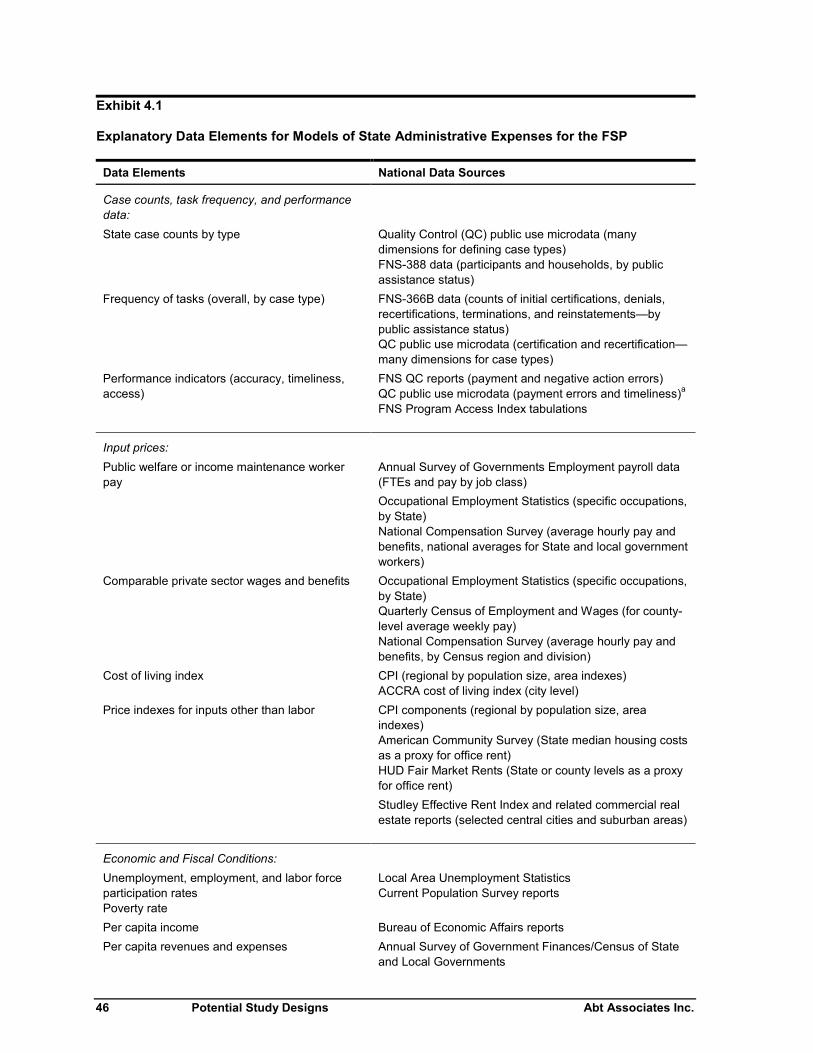
46 Potential Study Designs Abt Associates Inc.
Exhibit 4.1
Explanatory Data Elements for Models of State Administrative Expenses for the FSP
Data Elements National Data Sources
Case counts, task frequency, and performancedata:
State case counts by type Quality Control (QC) public use microdata (manydimensions for defining case types)FNS-388 data (participants and households, by publicassistance status)
Frequency of tasks (overall, by case type) FNS-366B data (counts of initial certifications, denials,recertifications, terminations, and reinstatements—bypublic assistance status)QC public use microdata (certification and recertification—many dimensions for case types)
Performance indicators (accuracy, timeliness,access)
FNS QC reports (payment and negative action errors)QC public use microdata (payment errors and timeliness)a
FNS Program Access Index tabulations
Input prices:
Public welfare or income maintenance workerpay
Annual Survey of Governments Employment payroll data(FTEs and pay by job class)
Occupational Employment Statistics (specific occupations,by State)National Compensation Survey (average hourly pay andbenefits, national averages for State and local governmentworkers)
Comparable private sector wages and benefits Occupational Employment Statistics (specific occupations,by State)Quarterly Census of Employment and Wages (for county-level average weekly pay)National Compensation Survey (average hourly pay andbenefits, by Census region and division)
Cost of living index CPI (regional by population size, area indexes)ACCRA cost of living index (city level)
Price indexes for inputs other than labor CPI components (regional by population size, areaindexes)American Community Survey (State median housing costsas a proxy for office rent)HUD Fair Market Rents (State or county levels as a proxyfor office rent)
Studley Effective Rent Index and related commercial realestate reports (selected central cities and suburban areas)
Economic and Fiscal Conditions:
Unemployment, employment, and labor forceparticipation ratesPoverty rate
Local Area Unemployment StatisticsCurrent Population Survey reports
Per capita income Bureau of Economic Affairs reports
Per capita revenues and expenses Annual Survey of Government Finances/Census of Stateand Local Governments
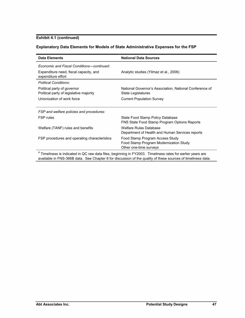
Abt Associates Inc. Potential Study Designs 47
Exhibit 4.1 (continued)
Explanatory Data Elements for Models of State Administrative Expenses for the FSP
Data Elements National Data Sources
Economic and Fiscal Conditions—continued:
Expenditure need, fiscal capacity, andexpenditure effort
Analytic studies (Yilmaz et al., 2006)
Political Conditions:
Political party of governorPolitical party of legislative majority
National Governor’s Association, National Conference ofState Legislatures
Unionization of work force Current Population Survey
FSP and welfare policies and procedures:
FSP rules State Food Stamp Policy DatabaseFNS State Food Stamp Program Options Reports
Welfare (TANF) rules and benefits Welfare Rules DatabaseDepartment of Health and Human Services reports
FSP procedures and operating characteristics Food Stamp Program Access StudyFood Stamp Program Modernization StudyOther one-time surveys
a Timeliness is indicated in QC raw data files, beginning in FY2003. Timeliness rates for earlier years areavailable in FNS-366B data. See Chapter 8 for discussion of the quality of these sources of timeliness data.
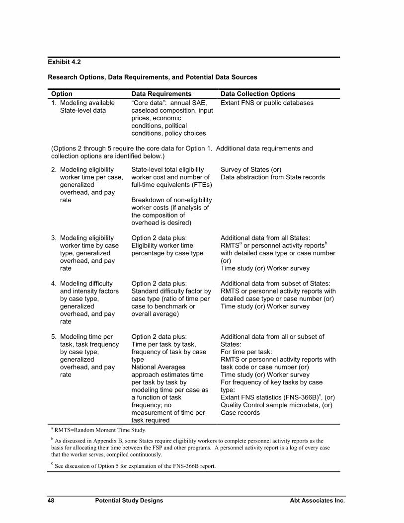
48 Potential Study Designs Abt Associates Inc.
Exhibit 4.2
Research Options, Data Requirements, and Potential Data Sources
Option Data Requirements Data Collection Options1. Modeling available
State-level data“Core data”: annual SAE,caseload composition, inputprices, economicconditions, politicalconditions, policy choices
Extant FNS or public databases
(Options 2 through 5 require the core data for Option 1. Additional data requirements andcollection options are identified below.)
2. Modeling eligibilityworker time per case,generalizedoverhead, and payrate
State-level total eligibilityworker cost and number offull-time equivalents (FTEs)
Breakdown of non-eligibilityworker costs (if analysis ofthe composition ofoverhead is desired)
Survey of States (or)Data abstraction from State records
3. Modeling eligibilityworker time by casetype, generalizedoverhead, and payrate
Option 2 data plus:Eligibility worker timepercentage by case type
Additional data from all States:RMTSa or personnel activity reportsb
with detailed case type or case number(or)Time study (or) Worker survey
4. Modeling difficultyand intensity factorsby case type,generalizedoverhead, and payrate
Option 2 data plus:Standard difficulty factor bycase type (ratio of time percase to benchmark oroverall average)
Additional data from subset of States:RMTS or personnel activity reports withdetailed case type or case number (or)Time study (or) Worker survey
5. Modeling time pertask, task frequencyby case type,generalizedoverhead, and payrate
Option 2 data plus:Time per task by task,frequency of task by casetypeNational Averagesapproach estimates timeper task by task bymodeling time per case asa function of taskfrequency; nomeasurement of time pertask required
Additional data from all or subset ofStates:For time per task:RMTS or personnel activity reports withtask code or case number (or)Time study (or) Worker surveyFor frequency of key tasks by casetype:Extant FNS statistics (FNS-366B)c, (or)Quality Control sample microdata, (or)Case records
a RMTS=Random Moment Time Study.b As discussed in Appendix B, some States require eligibility workers to complete personnel activity reports as thebasis for allocating their time between the FSP and other programs. A personnel activity report is a log of every casethat the worker serves, compiled continuously.c See discussion of Option 5 for explanation of the FNS-366B report.
Abt Associates Inc. Potential Study Designs 49
Option 2: Analysis of Overhead and Eligibility Worker Time perCase
Based on Equation 3.8, variation in SAE per case can be divided into three components: eligibilityworker time per case, eligibility worker pay (or a market equivalent), and generalized overhead(computed as the ratio of total costs to eligibility worker costs). Estimates from a model of this formcould be used to estimate the proportion of variation that can be attributed to each of thesecomponents, by holding two components at mean values and estimating the variance in the predictedcost based on actual variation in the remaining component.
Each component can be modeled separately. Eligibility worker time per case can be modeled as afunction of case characteristics and economic, political, and policy variables. Overhead can bemodeled as a function of economic, political, and management variables. If data were sufficientlydetailed, overhead would be further broken down between the local and State levels or on otherdimensions, to determine what portion of overhead varies the most and to facilitate more focusedmodels. Models of eligibility worker pay would focus on economic and political conditions.Eligibility worker experience might also be a factor in modeling both time per case and pay.
Other than the core data, this model requires the decomposition of SAE into eligibility worker costsand other costs. There are several options for estimating eligibility worker costs.
States may have FSP eligibility worker costs as a separate line item or cost center in theircomputation of total SAE.
The total eligibility worker cost for all programs may be a line item in the local office costallocation pool. (See Appendix B for explanation of cost allocation pools.) The FSP’spercentage of this pool (typically based on eligibility worker time distribution) can be appliedto the total eligibility worker cost to estimate the FSP cost for eligibility workers alone.
Time use data for eligibility workers from time sheets or random moment studies can be usedto determine the total eligibility worker time for the FSP. The average pay can be used toestimate the cost of this time.
For any of these options, some proxy for average eligibility worker pay is needed. For the first twooptions, average pay per eligibility worker hour can be computed as the ratio of total pay to eligibilityworkers to the number of eligibility worker hours assigned to the FSP. These hours could be adjustedfor pay differentials from the market by using a pay rate for a comparable occupation or broaderoccupational group.
There are two possible approaches for collecting information on eligibility worker time and pay. Oneapproach would be to request existing documentation from the States. The other approach is toprovide standard definitions of the measures and request that the States provide estimates. Both ofthese approaches could be implemented via mail, the Web, or a combination of these approaches withtelephone follow-up. The feasibility of these approaches is addressed in Chapter 6.
A key issue to be considered in this approach is obtaining consistency in the definition of “eligibilityworker” costs and pay. Job classifications may vary across States; so may the actual practiceregarding the types of workers that conduct certification interviews and make determinations of
50 Potential Study Designs Abt Associates Inc.
eligibility and benefits. Inconsistencies in the definition of eligibility worker costs could distort orconceal the actual differences among States. This issue is addressed in Chapter 6.
Another issue is whether to expand the data collection so that the “overhead” can be decomposed foranalysis. A logical breakdown would be between local office labor (excluding eligibility workers),other local office costs, and State costs. This approach would allow use of different wage or priceindexes to analyze variation in components of overhead. For example, variation in total overheadwould be modeled with a general cost index, such as the CPI or the ACCRA cost of living index (asreferenced in Exhibit 4.1). If the data are sufficiently detailed that rent is broken out, an index of realestate costs can be used for modeling variation across States. (We have not identified a public indexof commercial real estate costs computed at the State level. Instead, we have identified the indexes inExhibit 4.1, which are based on housing costs and should reflect the same underlying economic forcesthat affect commercial real estate costs, at least in terms of major differences among States.) Thefeasibility of collecting data on the composition of overhead is discussed in Chapter 7.
Option 3: Analysis of Cost by Case Type
This option would decompose costs as in Option 2, and then break down eligibility worker time bytype of case, using dimensions such as the presence of earnings or public assistance. Modeling theaverage time per case separately by case type would eliminate the need to include proxies for casemix as regressors in the models, conserving degrees of freedom. Instead, the models would focus oneconomic, demographic, political and policy variables. As in Option 2, overhead and eligibilityworker pay would be broken out and modeled separately. Anticipating our discussion of Option 4directly below, we emphasize that for Option 3 we envision collecting this information for every Statefor multiple years.
Obtaining cost data by case type for eligibility workers would provide a richer base for analyzingvariation in SAE than Options 1 and 2, but this option requires data that may not be easy to obtain.The required cost data are: eligibility worker time by case type, average eligibility worker pay, andtotal SAE. The time data could be collected from extant sources or by conducting a time-use study.
In some States, personnel activity reports or random moment study data may indicate the eligibilityworker time by case type. (This information might be in the form of a percentage, in which case thetotal eligibility worker time would be needed.) In particular, these sources tend to differentiate timeby program or program combination, as needed for cost allocation. On the other hand, data collectedfor this Feasibility Study suggest that other dimensions of case heterogeneity (e.g., presence ofearnings) are not identified in routinely collected data on eligibility worker time use, as discussed inChapter Six. In addition, detailed time use data are not routinely collected for FSP-only eligibilityworkers, because there is no need to allocate their time by program.
There is another option for using extant data to obtain a breakdown of time by case type for allworkers in a State. Personnel activity reports and random-moment time study data often include acase number for each instance of work recorded. This number could be matched to case records toassign a case type to the observation. The time use data could then be tabulated by case type, withadjustment for non-case time (breaks, meetings, etc.). An issue with using existing time studies isobtaining data on the mix of case types for FSP-only eligibility workers (as noted above).
Abt Associates Inc. Potential Study Designs 51
Several methods might be used to generate new data on eligibility worker time use by case type whenextant sources are insufficient. These include (a) modifying existing time studies to include a casetype indicator, (b) “job tickets” on which workers record all time spent on specified cases; (c) “eventlogs” recording each task with the case type and time spent for a designated period (as done byHamilton et al., 1989); or (d) worker surveys (also used by Hamilton et al., 1989).
The key feasibility issues for Option 3 are:
How should case types be defined, and what does this imply for the approach—in terms ofthe data collection burden and in terms of the gain in analytic insight?
Do most or all States collect data on eligibility worker time by case type? If so, what casetypes are identified? And, how far back is the information available?
Do most or all States collect case numbers as part of the data on eligibility worker time use?Is it feasible in practice to merge time use records with case records?
Are all of the data collected on eligibility worker time use entered in electronic files? Howlong are these files retained? Ideally, extant data could be collected for several years for time-series analysis.
Are extant data on eligibility worker time by case type comparable across States? What is theextent of error in these data?
Is new data collection on eligibility worker time by case type in all States feasible,considering the sample size needed, burden on workers and administrators, potential for error,and cost of collecting the data?
As discussed in Chapter 6, there are significant challenges to the feasibility of Option 3. Thediscussion there suggests that data for the likely case types of interest (e.g., working single parentwith children) exist in few States at most, and collecting such data in all States would be prohibitivelycostly and burdensome. By far the most feasible approach is to collect extant data on eligibilityworker time by program combination. Even that minimal approach appears likely to be constrainedby record retention and burden considerations. The next two sections of this chapter suggestalternative approaches that would disaggregate eligibility worker time with data that appear morefeasible to obtain.
Option 4: Analysis of Overhead, Difficulty, and Intensity by CaseType
Given that detailed data on costs by case type seem unlikely to be available for most States and years,how might we proceed? Equation 3.9 provides a starting point. We note that aggregate-level data oncase mix (for various definitions of case type) appears to be available for all States and all years. Ifwe knew the relative difficulty of each case type (and that difficulty was constant across States andyears), then we could replace the proxies for case mix in our reducted form models with a singledifficulty index. Total inputs per case would then be the product of this difficulty index and a proxyfor intensity; i.e., resources per standardized case. By replacing the proxy variables for case mix witha single difficulty index, this approach would conserve degrees of freedom and increase the precisionof the estimates of other factors.
52 Potential Study Designs Abt Associates Inc.
The challenge is then to construct the difficulty index. Discussion later in this report suggests that thequality of State data varies widely. It seems likely that in a subset of States and years, it will bepossible to estimate resources by case type. This information can be used to construct a difficultyindex. The difficulty index thus provides a way to exploit the data in the States and years with thebest data for analysis of the full time series of States and years.
Having controlled for case mix using the difficulty index, separate regression models would attemptto explain variation in overhead, intensity, and pay. This decomposition can be used to determine theproportion of variation due to differences in case mix and pay (largely uncontrollables, albeit withsome secondary effects from State choices) and overhead and intensity (mostly or largely due tocontrollables). As described in Chapter 3, normalized costs (setting difficulty and pay to nationalaverages) could be used to investigate the relative efficiency of States and the relationship of costs toState performance.
The data requirements for Option 4 are the same as for Option 2, plus the data for the difficulty index.The difficulty index by case type ideally would be computed from data on eligibility worker time percase by case type. The difference between Options 3 and 4 is that Option 3 assumes collection oftime by case type for all States for the study time period, while Option 4 would collect thisinformation from a sample of States and possibly a subset of study years. If collecting worker timeby case type along the lines of Option 3 would require a new time study in most States (as seems tobe true), then Option 4 leverages existing data on time by case type from States that can provide it,and then generalizes that information to all States.
There are four basic data collection methods that might be used in a sample of States for Option 4:
Existing data on eligibility worker time by case type could be obtained from States thatcollect the data in random-moment time studies or personnel activity reports.
Existing random-moment time studies or personnel activity reports could be modified toinclude case type codes for observed moments.
Data from random-moment time studies or personnel activity reports with case numberscould be merged with case records to identify the case type for each observation.
A new time study could be conducted with a sample of workers in each State, using one ofthe methods listed under Option 3. Conducting such studies in a sample of States would beconsiderably more feasible than doing so in all States.
The feasibility issues for data collection under Option 4 are similar to those for Option 3, with thecrucial difference that data would be collected only in a sample of States and years, rather than for allStates and years. For existing data, the years are likely to be limited by data retention. For new datacollection, the only feasible year will be the year of the study. The issues for Option 4 include:
What are the case types of interest? How many observations for each case type are needed?
How many States are needed? Will they be stratified so that difficulty indexes can beestimated for different types of States?
What States have extant data that could be used? How representative are these States? Howcomparable are their data? What is the extent of error in these data?
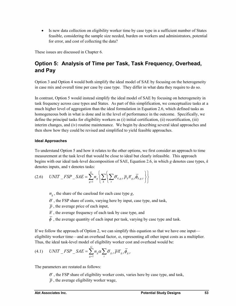
Abt Associates Inc. Potential Study Designs 53
Is new data collection on eligibility worker time by case type in a sufficient number of Statesfeasible, considering the sample size needed, burden on workers and administrators, potentialfor error, and cost of collecting the data?
These issues are discussed in Chapter 6.
Option 5: Analysis of Time per Task, Task Frequency, Overhead,and Pay
Option 3 and Option 4 would both simplify the ideal model of SAE by focusing on the heterogeneityin case mix and overall time per case by case type. They differ in what data they require to do so.
In contrast, Option 5 would instead simplify the ideal model of SAE by focusing on heterogeneity intask frequency across case types and States. As part of this simplification, we conceptualize tasks at amuch higher level of aggregation than the ideal formulation in Equation 2.6, which defined tasks ashomogeneous both in what is done and in the level of performance in the outcome. Specifically, wedefine the principal tasks for eligibility workers as (i) initial certification, (ii) recertification, (iii)interim changes, and (iv) routine maintenance. We begin by describing several ideal approaches andthen show how they could be revised and simplified to yield feasible approaches.
Ideal Approaches
To understand Option 5 and how it relates to the other options, we first consider an approach to timemeasurement at the task level that would be close to ideal but clearly infeasible. This approachbegins with our ideal task-level decomposition of SAE, Equation 2.6, in which g denotes case types, kdenotes inputs, and τ denotes tasks:
(2.6)
G
g kgkgkgkg pnSAEFSPUNIT
1,,,,,__
gn , the share of the caseload for each case type g,
, the FSP share of costs, varying here by input, case type, and task,p , the average price of each input, , the average frequency of each task by case type, and
, the average quantity of each input per task, varying by case type and task.
If we follow the approach of Option 2, we can simplify this equation so that we have one input—eligibility worker time—and an overhead factor, , representing all other input costs as a multiplier.Thus, the ideal task-level model of eligibility worker cost and overhead would be:
(4.1)
G
ggggg pnSAEFSPUNIT
1,,,__
The parameters are restated as follows:
, the FSP share of eligibility worker costs, varies here by case type, and task,p , the average eligibility worker wage,
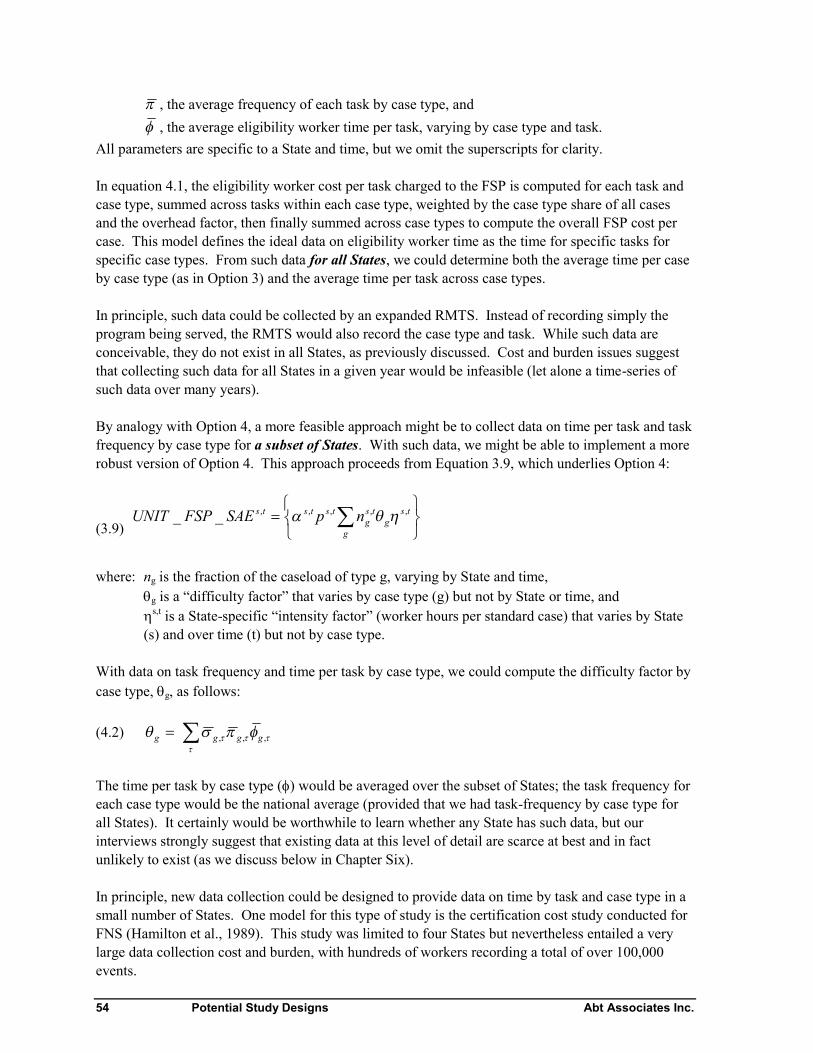
54 Potential Study Designs Abt Associates Inc.
, the average frequency of each task by case type, and
, the average eligibility worker time per task, varying by case type and task.All parameters are specific to a State and time, but we omit the superscripts for clarity.
In equation 4.1, the eligibility worker cost per task charged to the FSP is computed for each task andcase type, summed across tasks within each case type, weighted by the case type share of all casesand the overhead factor, then finally summed across case types to compute the overall FSP cost percase. This model defines the ideal data on eligibility worker time as the time for specific tasks forspecific case types. From such data for all States, we could determine both the average time per caseby case type (as in Option 3) and the average time per task across case types.
In principle, such data could be collected by an expanded RMTS. Instead of recording simply theprogram being served, the RMTS would also record the case type and task. While such data areconceivable, they do not exist in all States, as previously discussed. Cost and burden issues suggestthat collecting such data for all States in a given year would be infeasible (let alone a time-series ofsuch data over many years).
By analogy with Option 4, a more feasible approach might be to collect data on time per task and taskfrequency by case type for a subset of States. With such data, we might be able to implement a morerobust version of Option 4. This approach proceeds from Equation 3.9, which underlies Option 4:
(3.9)
g
tsg
tsg
tststs npSAEFSPUNIT ,,,,,__
where: ng is the fraction of the caseload of type g, varying by State and time,g is a “difficulty factor” that varies by case type (g) but not by State or time, ands,t is a State-specific “intensity factor” (worker hours per standard case) that varies by State(s) and over time (t) but not by case type.
With data on task frequency and time per task by case type, we could compute the difficulty factor bycase type, g, as follows:
(4.2) g
,,, ggg
The time per task by case type () would be averaged over the subset of States; the task frequency foreach case type would be the national average (provided that we had task-frequency by case type forall States). It certainly would be worthwhile to learn whether any State has such data, but ourinterviews strongly suggest that existing data at this level of detail are scarce at best and in factunlikely to exist (as we discuss below in Chapter Six).
In principle, new data collection could be designed to provide data on time by task and case type in asmall number of States. One model for this type of study is the certification cost study conducted forFNS (Hamilton et al., 1989). This study was limited to four States but nevertheless entailed a verylarge data collection cost and burden, with hundreds of workers recording a total of over 100,000events.
Abt Associates Inc. Potential Study Designs 55
An alternative would be an expanded RMTS collecting task type and case type (or case number,allowing case type to be determined from case records). Such a study could be designed to be lessintrusive than the methods used in the FNS certification cost study, while collecting data across theentire State and thus avoiding distortions due to local office conditions. The number of observationswould depend on several design considerations: the number of tasks, the number of case types, theway that the data would be analyzed, and the expected level of precision of the estimates.33
Thus, analysis of costs by task and case type is technically feasible, and FNS could learn much fromsuch a study. The cost and total burden on workers, however, would be high. Therefore, we presentsimpler and less costly approaches below.
Simplified Approaches
Relative to the ideal approaches to analyzing eligibility worker time by task, Option 5 woulddramatically reduce the data requirements and simplify the analysis of eligibility worker time byassuming that time per task does not vary by case type. Following the approach of Equation 3.10,Option 5 would disaggregate the overall variation in eligibility worker time per case as charged to theFSP into four components: differences in time per task (by task only), in task frequency (for eachtask by case type), in FSP share of costs by case type, and in case mix.34 Recall that Equation 3.8decomposes FSP cost per case into overhead (, eligibility worker pay (p) and eligibility workertime per case (w).
(3.8) tstststs wpSAEFSPUNIT ,,1
,,__
(3.10) tstsg
tsg
gg
ts nw ,.,
,,
Equation 3.10 defines eligibility worker time per case as a function of case mix (ng), FSP cost share(σg) by case type, task frequency by task and case type (g,), and time per task varying only by task().
Under this approach, the sample required to estimate the overall average time for a task (across allcase types) would be a fraction of the sample required for time per task varying by case type. Inprinciple, this option might be implemented with existing data or with new data collection on a moremodest scale than the 1989 certification cost study.
With individual data on eligibility worker time for specific tasks in all States for the years of interest,we could apply an approach analogous to Option 3. We could separately model the time for each taskas a function of State characteristics other than case mix (such as whether workers who do the task
33 The most demanding approach, in terms of sample size, would be to estimate the mean time per task bycase type, since each task-case type combination would require an adequate sample, and the total samplewould be driven by the frequency of the least common combination of interest. In the approach ofHamilton et al., time per task was regressed on case characteristics, so the required sample was not as large.
34 The time per task is the total time that the worker spends. If a case participates in the FSP and anotherprogram, the time charged to the FSP is the product of the total time and the FSP share for this case type.For simplicity, we specify the FSP share as varying only by case type, as discussed in Chapter 3.
56 Potential Study Designs Abt Associates Inc.
are specialists or generalists). We could model task frequency by case type as a function of otherState characteristics (unemployment rate, poverty rate, etc.). We call this the “All States” version.
Alternatively, if we only had such data for a subset of States and years, we could proceed by analogywith Option 4. First, we transform (3.10) to express the time per case as the sum of time over tasks.
(4.3) tsg
tsg
gg
tsts nw .,
,,,
Each task has a weight based on case mix, FSP share by case type, and the frequency of the task bycase type.
The analysis must take into account the fact that eligibility workers do not spend all of their time ontasks for individual cases. They attend meetings and training, do general paperwork, and carry outother non-case-specific tasks. We can account for this by defining a “task” representing the share ofthis non-case time attributable to the average case (and thus included in w); RMTS are designed tomeasure this time and can provide this information.
From the States and years with the best data, we could estimate the time per task for each task andtreat this as a constant across States (i.e., we drop the s and t superscripts for ). We call this the“Subset of States” version. Assuming information on tasks performed (at some level of aggregation),case mix, and FSP cost share were available for all States and years, we could then estimate the
expected time per case for each State ( tsw ,ˆ ) required to perform the tasks per case observed in aState. Then for each State we would compute a measure of intensity using the actual and expectedtime per case, as in (4.4):
(4.4) ts
tsts
ww
,
,,
ˆ
Note that the States chosen do not have to represent the average time per task across States; theymerely provide the basis for comparisons of effort relative to the weighted frequency of tasks. We
could also estimate tsw ,ˆ using the average frequency of tasks by case type for all States. Combinedwith the other information from this approach, we could determine the share of variation in time percase attributable to heterogeneity in case mix, FSP share, task frequency, and intensity.
A less data-intensive approach to Option 5 would estimate national averages for the time per task andcombine these estimates with State-level task frequency by case type. We call this the “NationalAverages” approach. This approach would begin with State-level estimates for eligibility workertime per case, based on the method of Option 2. No additional time use data would be needed.Instead, the national average time per task for each task would be estimated with a regression modelof State estimates of eligibility worker time per case as a function of the frequency of tasks for allcase types combined.35 (Aggregating across case types would be crucial to the feasibility ofestimating this model, particularly if the time per task does not in reality vary by case type.) Thismodel would be estimated for tasks 1 through n as in (4.5).
35 This is analogous to the production function approach to estimation of costs of school breakfasts andlunches based on numbers of meals served and school districts’ total costs (see Bartlett et al., 2008).
Abt Associates Inc. Potential Study Designs 57
(4.5) tstsnn
tstsw ,,,11
, ...
The coefficients () estimated in (4.5) thus represent the contribution of each task to the total time percase. The linear specification is clearly appropriate: time per case is the sum of time over tasks.Note that a constant term could be added to represent a fixed cost per case for non-case-specific time.We can use the estimated average values of in 4.3 to estimate each State’s eligibility worker
expected time per case ( tsw ,ˆ ) and its intensity (as in 4.4). As in the Subset of States version, wecould also compute the expected time per case using the national average task frequency by case type.Taken together, these estimates will allow analysis of the effects of caseload composition, taskfrequency, and intensity on eligibility worker time per case.
There is an important benefit of decomposing time per case into the product of time per task and taskfrequency by case type. This allows the generalization of time per case under particular conditions toother conditions, as done by MaCurdy and Marrufo (2006). In particular, if the task frequency wouldbe different but the time per task would not, then task frequency data can be used to estimate the timeper case. Case records provide a rich source of existing task frequency data, and more limited taskinformation is available in QC data derived from these records, whereas time per task data appear tobe scarce.
Potential Estimation Approaches
There are several potential approaches to estimating time per task and task frequency. For each State,time per task could be estimated in several different ways:
using extant data from States where RMTS or personnel activity report data includeindicators for the task, or where these data could be merged with case records indicating thetask performed at the time recorded
conducting a new time study, using an expanded RMTS or event logs (i.e., recording time onevery task for a period up to a month)
a worker survey, process observation, interviews with key informants, or some combinationof these “low impact” approaches with less burden on individual workers than a time study.
The choice among these alternatives would depend on (a) the availability and quality of the extantdata, (b) the number of States to be included (all States or a subset, size of subset), and (c) the feasiblelevel of cost and burden for the study. Under the National Averages approach, no additional datacollection on time per task would be needed, but the estimates would be national, not State-specific.
There are four ways to estimate task frequency by case type for a State:
combine records of individual tasks with the characteristics of the affected case fromcomputerized case records;
impute incidence of tasks from comparisons of case records over time, and combine thisinformation with case type information from the case records;
58 Potential Study Designs Abt Associates Inc.
estimate the frequency of identifiable tasks by case type using Quality Control (QC) sampledata for each State (which identify active cases with initial certification, recertification, and(for some years) interim actions in the sampled month); or
use the task counts reported by the States on the FNS-366B report, which includes counts ofinitial applications approved, applications denied, recertifications, and terminations. Thesecounts are broken down between households with and without public assistance.
These methods are described and assessed in Chapter 6.
The key feasibility issues for Option 5 are:
What States have extant data that could be used? How representative are these States? Howcomparable are their data? What is the extent of error in these data?
Is new data collection on eligibility worker time by task in a sufficient number of Statesfeasible, considering the sample size needed, burden on workers and administrators, potentialfor error, and cost of collecting the data?
What are the potential challenges of using State case records to estimate task frequency bycase type? What does this imply for the feasibility of the State-level approach to Option 5 inall States or a sample of States?
What is the feasibility of using the QC microdata to estimate task frequency by case type?What are the limitations of these data, and what does this imply for the analysis?
What are the potential limitations of using the FNS-366B data to estimate task frequency bycase type, and what does this imply for the analysis?
We address these issues in Chapter 6, which provides an overall assessment of the feasibility of theseoptions. Before we do so, we consider the fundamental issue of whether SAE for the FSP as reportedto FNS is sufficiently comparable across States and over time to justify the effort that these optionsmight require.
Abt Associates Inc. Comparability of Aggregate Reported Expenses 59
PART II: ASSESSMENT OF DATA SOURCES FOR POTENTIAL
STUDY DESIGNS
In this part of the report, we present the results of our data assessment. In Chapter 5, we consider thebasic question of whether aggregate SAE, as reported to FNS, is sufficiently comparable across Statesto permit valid analysis using the approaches described in the previous chapters. In Chapter 6, wefocus on the feasibility of collecting the data that these approaches would require on eligibility workertime, compensation, and costs. In Chapter 7, we consider the data for decomposing and modelingcosts other than eligibility worker labor. Finally, in Chapter 8, we assess the sources and quality ofdata on potential explanatory variables for the proposed approaches. As discussed in Chapter 1, thisassessment is based on interviews with Federal and State officials, and on the researchers’ ownexperience with these data.
Chapter 5
Comparability of Aggregate Reported StateAdministrative Expenses
A natural approach to understanding SAE would be to use aggregate State expenses as reported toFNS. Study Option 1 is designed to use these data, which are readily available from FNS’ NationalData Bank. The other options would also use these data together with the States’ informationsupporting their reported expenses. This chapter considers the comparability of reported SAE dataacross States and across time. One of FNS’ reasons for conducting this study was to address concernabout the comparability of these data and the possible implications for the feasibility of analyzingvariation in SAE. The feasibility of all of the options depends on the quality of reported SAE.
To support comparative analysis, one would ideally have completely accurate—i.e., error-free—data.In this context, “error” refers to any situation in which the data used for allocation and reporting ofcosts do not reflect the actual use of resources. As such, the error may be random, or there may be anon-random bias. Random error would be unlikely to create consistent differences across States orover time, but it could make the true differences and their causes more difficult to detect. “Bias”refers to a persistent pattern of allocating more or less cost to a program than the share of theresources that the program actually used. The possibility of bias is a greater concern than the risk ofrandom error, because a bias would introduce spurious differences in cost across States or over time.
Potential Errors Arising in the Allocation and Reporting of SAE
In considering the possible reasons why reported SAE might not be comparable across States andover time, it is important to consider the key elements of the reporting process. First, the Statedisburses money for expenses: payroll, benefits, purchases of goods and services, and interagencypayments. Some of these expenses are assigned directly to the FSP or other programs; the rest go intoone or more joint expense pools to be allocated among programs. Meanwhile, the State gathers datanecessary to allocate the joint expenses. On a monthly or quarterly basis, the State computes the
60 Comparability of Aggregate Reported Expenses Abt Associates Inc.
share of joint expenses for each program, adds the directly assigned expenses, and reports thecombined administrative expenses for each program to the agency providing administrative funds.For the FSP, expenses are computed separately for the functional reporting categories and thentotaled.
FSP agencies allocate shared costs among their programs according to cost allocation plans. Theseplans consist of complex systems of cost pools (groups of related expenses allocated the same way)and rules to allocate costs. Expenses that are exclusively attributable to the FSP are directly chargedin the accounting system. These include workers who exclusively serve the FSP and services chargedseparately for the FSP, such as benefit issuance. Shared expenses for the FSP and other programsmay be allocated in proportion to measures of usage (percentage of hours, computer connect time,etc.). Finally, some shared expenses may be allocated in proportion to usage of other resources.This method is used for expenses for which it is infeasible or disproportionately burdensome todetermine usage by the FSP and other programs.
Most notably, costs for multi-program eligibility workers and other workers with direct client contactare usually allocated on the basis of random-moment time studies (as described in Appendix A), butsometimes these workers maintain “personnel activity reports” on a continuous basis. Percentages ofeligibility worker time or costs are often used to allocate costs for other local office personnel, non-personnel costs of local offices, and some State-level costs. Thus, the data and methods for allocationof eligibility worker costs are particularly important to the overall allocation of costs between the FSPand other programs.
Having accurate data for comparative analysis of SAE (as defined above) requires several conditions.States must disburse funds accurately for all allowable costs. (We have assumed that the possibilityof errors in disbursements is not a concern for this study.) State and local expenses must be allocatedacross programs by standard and equitable rules, the data used in the allocation must be measuredwithout error, and the computations for the allocation must be correct. Expenses must be reported byall States in the correct time periods and reporting categories.
There are several ways in which cost allocation and reporting could deviate from the ideal conditions,thus undermining the validity of comparisons of reported SAE across States:
1. Cost allocation plans could be designed in a way that, accidentally or otherwise, tends toallocate more or less costs to the FSP, relative to other plans. Such differences wouldmake the costs less comparable than if the same plan were used.
2. Errors in data collected for cost allocation or in carrying out cost allocation algorithmscould cause the actual cost allocation to diverge from the correct allocation. These errorscould be unbiased (i.e., random) or biased (shifting costs from some programs to others).
3. Reporting errors or inconsistencies could result in costs reported in the wrong category.
4. Lags in the accounting process could result in costs reported for the wrong time period.
These threats to the validity of comparisons are considered in the sections that follow. We firstconsider the question of what costs are to be compared (i.e. which FSP functions are to be included)and whether they are defined and reported consistently. Although reporting is the final stage in theaccounting process, these issues must be considered first in order to provide a context for the nextdiscussion, in which we assess the threats to the validity of comparisons from differences in how
Abt Associates Inc. Comparability of Aggregate Reported Expenses 61
costs are allocated across programs. Finally, we consider issues of the comparability of reportedexpenses over time. In general, we conclude that the SAE data are sufficiently comparable acrossStates to permit valid analysis, at least for FY1999 and later years, but that data quality issues mayaffect the ability to produce unequivocal results from simply analyzing aggregate SAE data, as inOption 1.
Definition and Comparability of Reported Expenses for FSPFunctions
A major threat to the validity of comparisons of SAE is that differences in definition could distortcomparisons of reported expenses for specific functions, such as certification. Reported SAE for theFSP includes the costs of all of the FSP functions. The functional cost categories are:36
certification issuance quality control management evaluation fraud control automated data processing (ADP) operations and development fair hearings employment and training (E&T) outreach nutrition education (FSNE) reinvestment (i.e., State spending required under an agreement to defer payment of sanctions
for excessive errors) System for Alien Verification of Eligibility (SAVE) unspecified other
These functions have different objectives, use different production processes, and usually areperformed by different organizations. Therefore, it is appropriate to model the costs of thesefunctions separately, provided that the functions are clearly defined and the costs can be separated.
Thus there are two issues about functional cost categories for designing studies of food stamp SAE:first, what are the theoretical categories of interest? and second, what are the actual categoriesfrom State expenditure reports to be used?
Functions of Interest for Analyzing Variation in SAE
For this report, we have assumed that certification is the most important functional category.Certification costs—as labeled in State reports—represent three-fifths of all SAE. (See Exhibit A-1for this and other percentages of total SAE by function.) Thus, the variation in total SAE cannot beexplained without explaining differences in certification costs. Certification policy is complex andgives States many options that may affect costs. For these reasons, the models discussed in this
36 The official definitions of the SAE reporting categories are provided in Appendix B.
62 Comparability of Aggregate Reported Expenses Abt Associates Inc.
report focus on certification costs, particularly in their emphasis on eligibility worker costs and theirspecification of the roles of case mix and certification policy variables.
We also assume that data processing costs are another area of interest. As noted previously, there arepotential trade-offs between eligibility worker costs and automated data processing costs.
Although expenditures on services to clients other than certification are an important part of the FSP,different frameworks are needed to study variation in their costs. Studies of EBT costs for FNS haveidentified a very different set of variables, such as recipient shopping patterns and the proportion ofretailers equipped at government expense to process EBT transactions (Phoenix MAXIMUS, 2000).For modeling FSNE and E&T costs, the important factors would include program design,participation levels (in total or as a percent of all food stamp participants), the type of agency servingas the subgrantee, and the types of partners. Fraud control costs include the establishment andrecovery of claims for overpayments, and investigation and prosecution of fraud; these costs would bemodeled on the basis of the volume of claims and investigations, and the types of staff and otherresources used. In order to keep this feasibility study focused, it is necessary to set aside thefeasibility issues for analyzing variation in these costs. We also assume that explaining variation inthe costs of oversight functions is not a priority; these include quality control, managementevaluation, and fair hearings.
Therefore, in this chapter and those that follow, we focus on the direct and indirect costs ofcertification (as defined in the following section), and on separating these costs from the other clientservice functions (issuance, E&T, and FSNE). In the discussion that follows, “direct” costs are thecosts of interacting with customers (applicants and participants). For certification, the primary directcost is the labor of front-line personnel; other direct costs include supplies and travel. Indirect costsare the costs of facilitating and overseeing these interactions: support staff, supervisors, managers,facilities, telecommunications, and other support services.37 Direct costs are specific to a function,while indirect costs are shared across functions. Automated data processing (ADP) costs could beviewed as an indirect cost of certification, but we treat them as a separate category because they arereported such, and because there may be interest in trade-offs between data processing and laborcosts.
FSP Cost Reporting Categories of Interest
In practice, States are not consistent in their definition of certification costs as reported on the SF-269expenditure reports, according to our interviews with FNS. In particular, some States include bothdirect and indirect costs of certification in the “certification” category, while other States report someor all indirect costs (supervision, facilities, State administration, etc.) elsewhere, such as in the“unspecified other” category. Analysis of data for 1989 to 2001 for a recent study showed asignificant negative correlation between certification and “unspecified other” costs within States,consistent with the views of FNS experts about the variation in reporting between these twocategories (Logan, Rhodes, and Sabia, 2006).
37 In cost allocation plans and related documents, “indirect cost” can have two meanings that differ from thedefinition that we use here. In one alternative definition, any cost that is not directly charged to a programis an “indirect cost”. Another definition is that an “indirect cost” is a cost that is allocated by an indirectcost (percentage) rate.
Abt Associates Inc. Comparability of Aggregate Reported Expenses 63
When defining which FSP reporting categories to include in an analysis of “certification” costs, thereis also the conceptual issue of whether to include activities that are consistently reported as separatecosts but contribute to the effectiveness of certification. This question is particularly important forpotential analyses comparing normalized costs to measures of accuracy, timeliness, and programaccess.
A broad definition of certification was used in the recent study of certification errors and costs(Logan, Kling, and Rhodes, 2008). The definition of certification-related costs included allcomponents of SAE except those that were clearly not related to certification (issuance, FSNE, andE&T). Thus, the measure included outreach, “unspecified other”, quality control, fraud control, fairhearings, reinvestment, and management evaluation costs. The authors noted that assignment of costsbetween certification and these related activities might vary across States, and that spending on therelated activities might contribute to the effectiveness of certification. The certification-related costmeasure excluded ADP costs on the grounds that these might trade off with certification costs andshould be considered separately. The authors tested an alternate measure of certification cost thatincluded ADP; this specification did not change the results. A separate variable for ADP costs had noeffect on the error index.
Discussions with FNS and the States suggest a standardized definition of certification costs foranalysis of SAE should at least include the costs reported by States in the certification, outreach,reinvestment, and “unspecified other” cost categories. Based on the known overlap of thesecategories in State reports, it is potentially misleading to separate them. The combination of thesecosts, however, appears to be comparable across States.38 Fraud control, fair hearings, andmanagement evaluation costs, in contrast, appear to be clearly defined as distinct from certification.These three categories could be excluded from a narrowly defined study of certification costs, or theycould be included because they are closely related to certification. The quality control (QC) expensecategory is also well-defined and could be kept separate, but QC provides feedback to improvecertification and thus should be considered if the analysis will relate certification costs to the accuracyof certification. A study of SAE could, of course, use multiple measures of certification costs. Also,we note that the differences among these alternative certification cost measures will be small. Fairhearings, management evaluation, reinvestment, outreach, and quality control expenses (as reported)jointly make up only about 3 percent of total SAE; fraud control represents 5 percent (Logan, Kling,and Rhodes, 2008).39
One practical issue with defining “certification” costs for analysis is whether to prorate the“unspecified other” costs between certification and the other functions (FSNE, E&T, issuance, andADP). On the one hand, it is likely that most “unspecified other” costs are indirect costs of
38 A State must have approval to conduct those activities that are defined as “outreach” in FSP rules, so thesecosts are likely to be clearly defined. However, these specified outreach activities can be a substitute forcertification costs: for example, community partners doing outreach can provide assistance withapplications in place of local FSP office personnel. This substitutability is the reason for recommendingthat outreach should be included in the definition of certification costs for analysis of SAE. Outreach inFY2006 cost less than $16 million, while the certification category alone totaled $3.3 billion, so thetreatment of outreach will not have much effect on analysis of certification costs.
39 These and most other percentages of total costs did not vary materially from year to year over the period ofthe study. The only notable changes in the percentage distribution were a decrease in the percentage for“unspecified other” and an increase in the percentage for nutrition education.
64 Comparability of Aggregate Reported Expenses Abt Associates Inc.
certification, because certification represents so much of the total SAE. Furthermore, to the extentthat the other functions are contracted out, the reported cost will include the provider’s direct andindirect costs. On the other hand, the categories other than certification may share the indirect coststhat may be included in “unspecified other” (e.g., State program management overseeing FSNE,E&T, and issuance as well as certification). A reasonable approach would be to assume that the vastmajority of indirect costs in “unspecified other” are certification-related, and therefore include the“unspecified other” costs in certification, but also to perform a sensitivity analysis using a proratedshare of these costs. The alternative would be to collect data to decompose the “unspecified other”,as discussed in Chapter Seven.
As suggested previously, there are arguments both for and against treating ADP costs as a componentof certification costs. On the one hand, if there is substitution of ADP costs for labor costs, it may belogical to consider ADP costs as part of the “overhead” as defined for Options 2, 3, 4 and 5. On theother hand, the primary factors that affect variation in ADP costs may be specific to this costcategory, such as the age and design of the ADP system. The choice between these arguments woulddepend on the objectives of the study and the data to be collected.
The rationale for treating ADP spending as a component of certification cost, or as a determinant ofcertification cost, depends on the assumption that ADP spending is related to the State’s level ofautomation. This would seem to be a reasonable assumption: a more capable ADP system would beexpected to cost more to develop and operate than a simpler system. The second assumption is that amore automated system reduces the labor required for certification. Without these relationships,variation in ADP costs might not be of much interest, since ADP costs represent only about 7.5percent of all FSP SAE (for 1989-2005, as reported in Logan, Kling, and Rhodes, 2008).40
Interviews for this study yielded much skepticism about whether these assumptions hold in practice.Experts suggested that the amount spent on ADP systems, particularly for development, has arelatively loose relationship to the gains in efficiency and accuracy that result from implementing newsystems. Thus, a profile of each system and its capabilities might be more useful than expendituredata for examining the relationship of ADP systems to certification costs. Such profiles wereformerly created and maintained by the Administration for Children and Families, Department ofHealth and Human Services (ACF), but these profiles have not been updated in recent years. FNS hasa great deal of information about the history of State ADP projects that might be mined, and iscurrently renovating its database on State ADP systems. A detailed investigation of these data wasbeyond the scope of this study but would be an important part of a study of ADP costs.
Whether data processing costs are analyzed separately from certification costs, or they are identifiedas a component of “overhead” for certification, there is an issue of how to define the measure of “dataprocessing costs”. States report two types of data processing costs—for operations and fordevelopment. Operational costs are the ongoing costs of operating and maintaining the dataprocessing system’s software, hardware, and communications networks. Development costs are theone-time costs of approved plans to create, renovate, or replace computer systems. These costs areclaimed on a cash basis, when they are incurred, even though the systems may be used for 10 years ormore thereafter. (One State interviewed for this study has a system that is 25 years old.) Thus, when
40 The share of annual costs for ADP ranged from 6.2 to 8.4 percent, with generally higher percentages after1996. (Source: unpublished tabulations from analysis files for Logan, Kling, and Rhodes, 2008.)
Abt Associates Inc. Comparability of Aggregate Reported Expenses 65
comparing data processing costs across States, or examining the tradeoff between data processing andcertification costs, we face the question of how to value the investment in developing data processingsystems. FNS has centralized records on the history of FSP information systems. These data mightbe used to identify the period when each State invested in its current system, so that this cost could beamortized over the life of the system. A simpler alternative is to analyze operations and developmentcosts separately, taking a cumulative approach to development costs.
Considering the issues regarding ADP costs, we do not recommend inclusion of these costs in ameasure of certification costs for comparisons across States and over time. We are also skepticalabout the value of treating ADP costs as an explanatory variable in analysis of certification costs.While the data exist and they could be used to model effects on certification costs (e.g., lagged ADPdevelopment spending as an explanatory factor), we believe that ADP costs should be betterunderstood before attempting such modeling. A descriptive study of ADP costs, the functions theysupport, and their relationship to system characteristics would be helpful to resolve the uncertaintiesabout how these costs fit into the bigger picture of FSP operations. In particular, such a study wouldhelp to formulate clearer expectations about how ADP system features and costs may be related tocertification costs.
Possible Biases and Random Errors in Allocation of SAE
Biases in the allocation of SAE could be unintentional or intentional. Unintentional bias could resultfrom consistent patterns of recall errors in self-reported data. For example, if workers do notmaintain time records on a timely basis and instead complete their reports by guessing how their timewas spent, their errors may not be random. They might tend to choose the first program on the list ofcodes (the primacy effect), the last program (the recency effect), or the program they work on mostoften (Schwartz et al., 2008). Intentional bias could be built into the algorithms for cost allocation, orit could be manifested in the choices and actions of State and local personnel as they gather data andimplement those algorithms.
If State and local agencies benefit more from some funding formulas than from others, they couldhave an incentive to charge to intentionally bias the allocation of costs toward the more favorablefunding sources. State assistance programs (such as supplements for the elderly, blind and disabled)receive no Federal funding, so there is a potential incentive to shift costs away from these programs toFederal programs. Medicaid provides more than half of the funding for State administrative expenses(60 percent on average in FY2004, according to CMS, 2008), and the Federal share varies amongStates. Thus, all States get more reimbursement for Medicaid SAE than for FSP SAE. States withhigher Medicaid Federal matching percentages may have a greater incentive to bias cost measurementand allocation toward the Medicaid program. The TANF program provides a block grant of Federalfunds, and each State has a “maintenance of effort” (MOE) requirement based on 1994 non-Federalfunding for AFDC. This funding structure could create incentives to shift costs to or away fromTANF. On the one hand, costs that can be paid with available TANF block grant funds require noState match (beyond the specified level for MOE), as opposed to the open-ended 50 percent Stateshare in most categories for the FSP. On the other hand, if the State expects to spend all of the TANFblock grant, then any additional costs allocated to the FSP bring a 50 percent Federal match, insteadof a 100 percent non-Federal cost.
66 Comparability of Aggregate Reported Expenses Abt Associates Inc.
The Federal controls on the cost allocation process, as described in Appendix B, are meant to assurethat administrative costs in general are equitably allocated in proportion to the actual use of staff timeand other resources. These controls include: Office of Management and Budget (OMB) and Divisionof Cost Allocation (DCA) requirements for cost allocation plans and standards for acceptablemethods and the substantiation of data used for cost allocation; review of cost allocation plans byDCA, FNS and other agencies; State audits mandated by the Single Audit Act and OMB Circular A-133; and reviews and audits of cost allocation conducted by FNS and other Federal agencies. Statesrecognize the responsibility to assure the validity of data on which financial reports are based and thepotential liability if those data are found deficient. Thus, a major focus of Federal and State oversightis to assure that costs are allocated in ways that fairly reflect the resources used by each program. Tothe extent that cost allocation meets this standard in practice, the costs will be comparable acrossStates and over time, because they will accurately reflect actual resource use.
While independent validation of FSP SAE is beyond the scope of this project, it appears unlikely thatState differences in SAE are materially biased by the way that costs have been measured andallocated, at least since 1998. This conclusion is based on the controls in place and on the viewsexpressed by Federal and State officials, as discussed below. There is, however, some basis toquestion the comparability of SAE prior to 1998 with later years because of a legislative changedescribed later in this chapter. There are also some possible ongoing sources of bias in minorcomponents of SAE.
Below, we discuss the controls and possible sources of bias and random error in cost allocation forthe major components of SAE: local agency administration, other client services, automated dataprocessing, and State administration. The focus of this discussion is on potential differences in costallocation across States that could bias comparisons of SAE. We then discuss issues of comparabilityin cost allocation and reporting over time.
Local Agency Costs
The allocation of local agency administrative costs—the substantial majority of all FSP SAE—is amajor focus of the requirements for cost allocation plans, both from OMB and from DCA. Theserequirements are designed to assure that worker samples for RMTS are sufficiently large and random,that workers are adequately trained and supervised in recording their time, that reporting is timely,and that time records are auditable (e.g., requiring the recording of case numbers and certification byworkers). Time certification and reporting is reviewed by local supervisors, the State Food StampAgency, State auditors, and Federal reviewers.
For the majority of States, reliance on RMTS helps to assure the validity of reported local costs.41
When executed properly, there is less risk of workers making recall errors (intentionally or otherwise)than in an ongoing time-keeping system. This is because the reporting is for a specific moment, sothe worker has a clear instruction to record activity at the designated time, whether that activity iscase-related, more general work, or non-work time such as breaks or leave. The random and discretenature of an RMTS may also make it less likely that workers believe that how they report their timeaffects their agency’s funding, and thus they will be less prone to bias their responses. When costallocation is based on personnel activity reports, workers have a more general instruction to keep
41 There does not appear to be a central tabulation of which States use RMTS versus other methods, butFederal experts agree that RMTS is the most common method.
Abt Associates Inc. Comparability of Aggregate Reported Expenses 67
track of activity as contemporaneously as possible. With much more information to track, there aremore opportunities for error.
The validity of any time reporting system depends heavily on the ongoing compliance of the workerswith the system and the oversight by supervisors. With only a small number of activities for eachworker to record, it is comparatively easier for workers to take the time to record time properly, andfor supervisors to monitor and verify observations. Nevertheless, there is evidence of problems withRMTS from at least two States, where the USDA Office of Inspector General (OIG) found thatrandom-moment time study procedures were not followed and quality controls were not consistentlyimplemented (USDA-OIG, 2000 and 2001). In one report, the OIG concluded:
“Because of this [the deficiencies in the RMTS], there was reduced assurance that thereported county staff activities represented what the staff was actually doing at the sampledmoments and, therefore, the FNS reimbursement of over $18 million in administrative coststo the FSP for the third quarter of fiscal year 1999 was questionable.” (USDA-OIG, 2000,page i)
The burden on workers and supervisors is greater with the personnel activity report method, and thusthe risk of error is greater, because all workers must record all of their time continuously, not justsampled moments. North Carolina addresses this risk by training workers three times each year ontime reporting procedures, and by requiring supervisors to review time reports on a weekly basis.State officials acknowledge that some supervisors are less attentive to these reviews than others.
Mechanisms are available to reduce the possibility of error in time reporting. For RMTS, some Statesseek to reduce recall error by having another person or an automated system contact the worker at thesampled moment, rather than giving the worker a form some time before the sampled moment andcollecting it hours or days later. In Nevada, for example, supervisors observe 10 percent of thesampled moments to validate the data. Some local agencies that use personnel activity reportsautomate this process to improve compliance and reduce errors.
The limitations of personnel activity reports, as discussed above, raise the possibility that allocationof local labor costs may be biased, or at least less reliable, in States that rely on this method. Whilethe possibility of greater error with this method is clear, the existence of bias would still depend on aconsistent pattern of error overstating or understating the time spent on the FSP. While State or localadministrators might perceive an advantage from biasing local time reporting in one direction oranother, there would be less motivation for individual workers to bias their time reporting. Aconcerted effort by administrators to bias time reporting is conceivable but would be difficult toconceal from the various reviewers, and the downside risk if this pattern were detected would beconsiderable. These considerations and the views of Federal experts suggest that the risk ofsignificant bias in personnel activity reports is low, but the risk of error in this system is higher thanwith RMTS.
Considering the potential impact of the local agency time measurement system on the accuracy ofcost data at this level, it would be useful to collect data on the type of system used in each State aspart of a study of FSP SAE. A key question is how the data are collected (self-reported or by anobserver; in real-time or after the moment). As discussed in Chapter 9, we recommend a survey ofStates to collect this and other information as part of the proposed plan of studies on SAE.
68 Comparability of Aggregate Reported Expenses Abt Associates Inc.
For workers that are not covered by time reporting or RMTS, and for nonlabor costs, the choice ofallocation method could affect the share of costs charged to the FSP. The main options are (a) usingthe percentage of time charged to each program, and (b) using the percentage of costs. Either methodcan be justified as equitable, so neither can be considered “biased”, but they could have differentresults. If the average pay rate is similar for workers who mostly or always work on the FSP and forother workers, and if there is no real difference in the direct-charged nonlabor costs across programs,the cost allocation result will be the same. On the other hand, some respondents suggested that newworkers may start handling the FSP and then add other programs as they become more experienced.If so, the average cost per hour for FSP activities could be lower, and thus the percentage of costscharged would be less than the percentage of hours. Differences in direct-charged costs at the locallevel could also affect the allocation of supervisory labor and other shared costs (e.g., if there aremore local training costs for TANF than for the FSP).
Given the size of the FSP relative to most other programs, differences between the percentage ofhours and the percentage of costs for the FSP are likely to be small, and therefore the impact of thechoice of method on cost allocation is likely to be small. This difference should, however, beacknowledged, because it might be particularly relevant in analyses of the ratio of non-eligibilityworker costs to eligibility worker costs in Options 2, 3, 4, and 5. Thus, it would be useful for a studyof SAE to collect information on the methods used to allocate local costs, including workers coveredby time reporting or RMTS and other costs. This information could be obtained through a survey orby review of State cost allocation plans.
Administrative Costs for Other Client Services
Several types of client services seem unlikely to be subject to bias in cost allocation. EBT is almostalways a contracted service with separate charges for each program on the system (FNS, 2008b).Similarly, employment and training (E&T) is usually contracted out and thus costs are a direct chargeto the FSP and not subject to cost allocation among programs.42 For nutrition education, thesubgrantees (or implementing agencies) operate other programs as well, so they must establish a basisfor allocating their costs across programs. Since subgrantees typically must secure the non-Federalfunds to match Federal FSP funds on their own, and they must secure advance approval for nutritioneducation plans and budgets, there is a built-in restraint on the risk of overstating the total FSP shareof the subgrantees’ overall spending. There is some risk that FSNE costs could be shifted to otherFederal programs, but they have similar controls. In any case, as stated previously, the focus of thisfeasibility study is on certification-related costs, and so the reliability of EBT, E&T, or FSNE costs isnot a concern for the present study.
The use of call centers or other centralized units for certification functions is a relatively new area,and little information on allocation of these costs was available for this study. Information from thestudy States and Regions suggests that some such units track calls by program for allocation, whileothers use RMTS of call center staff. Both call counts and RMTS for call centers would be expectedto be reliable and largely free of bias. The call centers operated by the study States were limited toinformation and referral services, however, so other methods might be used in call centers that carryout certification functions.
42 The USDA OIG did find, however, that staff time and other administrative costs reported as spent on E&Twere inflated in one State (USDA-OIG, 2003).
Abt Associates Inc. Comparability of Aggregate Reported Expenses 69
Reporting of ADP Development and Operations Costs
Any effect of bias in allocating ADP costs on overall SAE must be small, because these costsrepresent only 7.5 percent of total SAE.43 Bias in ADP cost allocation would, of course, have muchmore impact on separate analysis of these costs. Controls to minimize bias for these costs appear tobe well-established and strong, although FNS experts caution that these controls have evolved andstrengthened over time. Proposed cost allocation methods are subject to close review as part of theAdvance Planning Document review process for ADP development, as well as the normal costallocation plan review process. Rate-setting for statewide data processing centers is subject to reviewby State auditors as well as State and Federal funding agencies; HHS oversight of ADP costs has beenreduced, however, by staffing reductions. Utilization statistics are generated by automated processes,and some States (such as North Carolina) have built cost allocation calculations into these processesto further reduce the possibility of error and streamline cost reporting. According to Federal officials,audits and financial reviews discovered some problems with overcharging Federal programs (e.g., byusing “prime” processing time for Federal programs and lower-cost time for State programs), butthese instances occurred many years ago.44 There is some risk that time reports by ADP developmentpersonnel may be biased toward Federal programs, and particularly toward programs with more than50 percent Federal funding (such as Medicare). However, budgets for these projects are reviewed byState and Federal officials, and States cannot claim reimbursement for more than the approvedbudget. Last, effort by non-technical personnel on ADP development projects may be under-reported, but this is mainly an issue of the reporting category rather than whether costs were chargedto the proper program. Thus, it appears that ADP costs for recent years can be compared withconfidence, but some caution is in order when comparing older costs.
State-Level Administrative Costs
State-level administrative costs include functions mandated by the FSP, program oversight, andgeneral administration. The mandated FSP functions appear to have modest costs: quality control,fair hearings, and management evaluation represent less than 3 percent of total SAE, and fraudcontrol represents 5 percent (Logan, Kling, and Rhodes, 2008). Cost allocation documents from thesampled States and interviews with officials indicate that program oversight and generaladministration also represent small shares of total SAE. Thus, any bias in allocation of State-leveladministrative costs is likely to have little if any detectable effect on total SAE, but would of courseaffect comparisons of these costs by themselves.
The allocation of State-level administrative costs appears to be the area where State methods differmost and thus could yield different results (i.e., States A and B use the same resources foradministration but report different costs because they allocate costs differently). Federal officialsnote that States generally seek to maximize Federal reimbursements by identifying all allowableadministrative costs in their cost allocation plans, but Federal officials only approve cost allocationplans if they meet the OMB A-87 criteria for reasonable, necessary and allocable costs. When Stateschoose the bases for allocating State-level administrative costs, they appear to have more flexibility
43 As estimated for 1989-2005 using inflation-adjusted costs (Logan, Kling, and Rhodes, 2008).44 The sources of this information did not specify when these problems were identified, but the history of
federal oversight goes back over three decades, and it appears that these problems with ADP operationscosts were identified in the early years of this oversight. The reliability of ADP development costs wasreportedly improved by changes implemented in 2002.
70 Comparability of Aggregate Reported Expenses Abt Associates Inc.
than when allocating local-level costs, but these bases must be justified to Federal officials. Asdiscussed in the context of local agency costs, use of FTEs (from RMTS, direct charges, and activityreports) could result in a different allocation from the results of using percentages of costs based onthe same sources. The complexity of cost allocation plans makes it difficult to predict howdifferences in allocation of State-level costs between two States would affect their bottom-line costsfor the FSP. In general, however, if local costs represent by far the largest part of total SAE, and iflocal cost allocation is driven by an objective and reliable RMTS, it is unlikely that differences inexactly how this information is used will yield large differences in State-level administrative costs.Thus, while information on how State-level costs are allocated might be useful in assessing thecomparability of these costs, it is not necessary for a broader study combining State and local-levelSAE.
Comparability of Reported SAE Over Time
One of the great advantages of using reported SAE data is that they are available for many years. Therecent study of certification costs and errors (Logan, Kling, and Rhodes, 2008) used data for 17 years,from 1989 to 2005. SAE data for earlier years are available from FNS data files and reports. Havingmany years of data would give added power to time-series analysis using the difference-of-difference(State fixed effects) approach, as discussed in Chapter 4.
Such methods require that the variables of interest are defined and measured consistently over theanalysis period. They also require that variables reported for the each time period represent the sametime period of actual activity in all States. The definitions of FSP functions for cost reporting havechanged little over time, and analysts can choose how to combine these functions. There are,however, problems posed by changes in cost allocation rules and by the timing of cost reporting, asdiscussed below.
Changes in Allocation of Administrative Expenses
Three major changes in the 1990’s affect the consistency of the definition and allocation of Stateadministrative expenses for the FSP. First, the enactment of TANF in 1996 replaced the open-endedFederal funding for half of AFDC expenses with the TANF block grant and the State MOErequirement. This changed the financial incentives affecting cost allocation (see the previousdiscussion of the possible cost-shifting incentives of the TANF block grant).
Second, the Agricultural Research, Extension, and Education Reform Act of 1998 (AREERA)required States to change their cost allocation methods. Previously, many States allocated shared(“common”) costs for AFDC/FS cases entirely to AFDC, under the “primary program” method ofallocation.45 AREERA required all States to use the “benefiting” program method, which splits theseshared costs between TANF and the FSP, starting in 1999. (According to ACF, a few States secureda court decision that allowed them to continue using the primary program method.) Thus, the FSPcost for a FS/TANF case would be greater than the cost for a FS/AFDC case, even if nothing elsechanged other than the method of cost allocation. States might have changed their cost allocationpractices before they were required to, because of the difference in funding between TANF and the
45 The “primary” program is the one that bears all of the common costs, such as completing portions of theapplication for benefits that are used by all programs. In this case, the primary program was AFDC.
Abt Associates Inc. Comparability of Aggregate Reported Expenses 71
FSP. Some FNS Regional offices indicated that there was a substantial shift of costs fromAFDC/TANF to the FSP as a result of AREERA, while others indicated that there was little change,and others were unsure because none of the respondents were involved with FSP financialmanagement when AREERA was implemented. State respondents generally could not recall howthis provision of AREERA affected their States.
Finally, AREERA reduced the Federal share of certification costs. Starting in FY1999, FNS has beenrequired to deduct an “offset” amount that is deemed to be included in the State’s TANF grantbecause of the way that the grant was set (GAO, 1999).46 Thus, the non-Federal share equals 50percent of the total certification cost plus the amount of the offset. The size of the offset for eachState depended on the amount of common costs for AFDC/FS cases charged to AFDC, which variedsubstantially among States. Offsets were established for 44 States, and the average was 17 percent ofthe Federal share of certification outlays in FY1994 (the base year for the computation).47 Thischange did not directly reduce the total funding for FSP certification. It is possible, however, thatsome States reduced their total certification spending so that the adjusted non-Federal share wouldmatch the available funds.
Because of these changes brought by TANF and AREERA, particularly the requirement to changecost allocation methods, it appears that reported SAE prior to FY1999 is not entirely comparable toSAE for later years. This poses an important issue for time-series analysis. On the one hand, it isdesirable to use all of the available data, because the power to detect the causes of variation increaseswith the number of years of data used. In support of this approach, the expected difference inallocated costs between the primary program method and the benefitting program method has shrunkalong with the decline in the proportion of FSP cases with AFDC/TANF. This percentage declinedfrom 34 percent in 1996 to 13 percent in 2006 (Logan, Kling, and Rhodes, 2008; Wolkwitz, 2007).Also, it would be possible to control for the effects of AREERA by using information from the offsetcomputations. These data could be used to create a variable representing the fraction of FSPcertification costs allocated to AFDC under the primary program method in the baseline year for theoffset computations. This information could also be used to adjust the pre-AREERA costs.48
On the other hand, the comparability problem may outweigh the usefulness of including pre-AREERA certification costs in a time-series analysis. Given the large proportion of FSP cases withAFDC in the years before AREERA, the impact of the choice of allocation method was substantial.The potential solution would substantially complicate the analysis. Furthermore, the value to begained from using these data may not be great, since there are now nine complete fiscal years of FSPoperations under AREERA (1999 through 2007).
46 TANF grants were set on the basis of AFDC funding for a base year. This funding included administrativecosts that were, in most States, at least partly allocated on the “primary program” method. Thus, the AFDCfunding included costs that would have been allocated to the FSP under the “benefiting program” method.As a result, a portion of the TANF grant was considered (under AREERA) to be duplicating thereimbursement under the FSP.
47 This estimate is based on computations for Logan, Kling, and Rhodes (2008) using data provided by FNS.48 A simple indicator for the pre-AREERA years would force a constant effect for all States. Given the
known variation in the offset, this would clearly overstate the change in some States and understate it inothers. A pre-AREERA effect for each State might be a viable approach.
72 Comparability of Aggregate Reported Expenses Abt Associates Inc.
This issue does not have to be settled prior to undertaking analysis, however. A reasonable approachwould first test the ability to model the variables of interest with the post-AREERA data. Next, thepre-AREERA data would be modeled, both with and without the suggested adjustment. Review ofthese results would help indicate whether it is preferable to pool the data for the two periods and howthis should be done.
Consistency in the Timing of Reported Expenses
A different issue of comparability arises because States report SAE on a modified cash basis. As aresult, outlays are reported in the quarter in which the State actually pays for goods and services.Thus, the cost for a service or product that is delivered in one quarter may appear in the next quarter’sexpenses.
Lags in the reporting of expenses could affect the comparability of SAE over time. A time lag couldbe an issue for analysis of trends within States, because changes in expenses would not occur in theperiod in which they would be expected to change, based on the variables driving the change (e.g., thecaseload falls in a quarter but expenses fall in the following quarter). Differences in lags acrossStates would make it difficult to analyze the impact of a common change across States over time.
The likelihood of a lag in reporting depends on the type of expense. Payroll costs are paid at leastmonthly, so the lag in these costs across periods is likely to be minimal. Some expenses are billedless often, however, so the costs for a quarter may not be representative of all of the resources usedduring the quarter (particularly the nonlabor resources). In States where counties administer the FSP,all local costs are typically paid by the State in the quarter after the quarter in which the County spentthe funds, so cost trends in such States will lag behind trends in caseloads or other factors that affectcosts. In fact, this lag can result in costs for activities in one fiscal year being recognized, underaccepted accounting rules, as part of the following year’s costs. The same lag in billing and paymentcan affect the timing of reporting versus actual activity for contracted services and interagencypayments at the State level, including statewide data processing centers, FSNE, E&T, and outreach.
A further complication of cost reporting is that there is an extended process of closing out andfinalizing the expenses for the year. States can liquidate obligated funds up to two years after the endof the fiscal year, so the State can “catch up” and assure that costs incurred during the year are paidwith funds for that year. Expenses can be revised downward at a later date on the basis of financialreviews or audits. Thus, SAE should be analyzed on an annual basis, and it is preferable to wait up totwo years after the end of the fiscal year before expenses are considered final.
Under Federal cost accounting rules, expenses should be charged against funds for the year in whichcosts are obligated. If States follow this principle, therefore, the “spillover” of costs reimbursedunder an interagency agreement should be limited to the one-quarter lag discussed above. It ispossible, however, for States to charge expenses to the wrong year, particularly if there is aparticularly long lag in the billing by a contractor or another agency, or if there is a delayedadjustment to billing. An OIG audit of one State found $8.5 million charged in FY2000 for a prioryear’s expenses (USDA-OIG, 2002). Interviews with FNS officials indicate that such problems arerare and small when they do occur.
Abt Associates Inc. Comparability of Aggregate Reported Expenses 73
Summary
Our principal findings about the comparability of reported SAE are as follows.
The “certification” reporting category does not provide a consistent measure across States,but this problem can be solved by creating an analytic measure that also includes the“unspecified other”, “reinvestment”, and “outreach” categories. A broader measure thatincludes related activities (such as quality control and management evaluations) may bedesirable for analyses relating certification costs to effectiveness.
There is substantial uncertainty about how to compare ADP costs, and this uncertainty shouldbe resolved before attempting to relate these costs to certification costs.
In general, it is unlikely that comparisons of local costs would be materially affected bydifferences in current cost allocation methods. There is some risk that local costs are lessaccurately reported when States use personnel activity reports instead of RMTS for multi-program staff. Information about how local costs are allocated in each of the States would bevery useful for interpreting comparisons of SAE across States.
There is a somewhat greater possibility that comparisons of State-level management andoversight costs might be affected by differences in cost allocation methods, but these costsare a relatively small portion of SAE.
There do not appear to be cost reporting issues that would affect comparisons of FSNE, E&T,and issuance costs across States. Changes in these FSP components (particularly EBTimplementation) would affect comparisons over time.
Changes in cost allocation rules must be taken into account in comparing certification costsprior to 1999 with later years. It is possible to make adjustments for these changes, but theseadjustments would complicate the modeling of changes in these costs over time.
There are notable time lags in the reporting of SAE. For most States, these lags will notaffect comparisons of final annual expenses. For States where counties administer the FSP,however, reporting lags may affect comparisons of expenses with other States and with trendsin explanatory variables.
In general, there appears to be sufficient consistency in the reporting of SAE for the FSP to permitvalid comparisons across States and over time. This conclusion applies to all components of SAE,and particularly to certification costs at the local level—the focus of the options presented in Chapter4. This consistency is due to the extensive controls at the State and Federal levels to assure thatclaims for reimbursement are accurate and that the allocation of costs across programs is equitable.The primary limitation is that comparisons of costs prior to 1999 with later costs may be affected bydifferences in cost allocation methods. Adjustments to mitigate this problem appear feasible, but theresults could be sensitive to the adjustment. The extent of this problem is an empirical question. Thecaveats above suggest a need for further information about allocation of costs at the State level andthe timing of expenditures and reporting where counties administer the FSP. With respect to the latterproblem, it seems likely that reasonable adjustments can be made.

74 Comparability of Aggregate Reported Expenses Abt Associates Inc.
Abt Associates Inc. Data on Eligibility Worker Time, Compensation, and Costs 75
Chapter 6
Data on Eligibility Worker Time, Compensation, andCosts
As discussed in Chapter 4, Options 2, 3, 4, and 5 would focus on eligibility worker costs, bothbecause they represent the largest component of SAE, and because of the importance of these workersto the integrity and accessibility of the FSP. In this chapter, we discuss the quality, limitations, andfeasibility of potential sources of data on eligibility worker time, compensation, and costs. While thecategory of “eligibility worker” primarily refers to workers who make eligibility determinations, forthis chapter we recognize that in practice these options may require data on costs for other workerswho perform some of the functions done elsewhere by eligibility workers. This expanded group ofworkers adds other workers have regular contacts with applicants and recipients (such as screeners),and workers (such as clerical staff) who do not have direct client contact but process eligibilityinformation (applications, verification documents, periodic status reports, change reports, etc.) on anindividual basis. Not all eligibility workers as defined above work in local assistance offices; thisbroad definition would include call center workers who perform certification tasks (as in Florida’smodernization of the FSP).
As indicated in Exhibit 4.2, Options 2, 3, 4, and 5 require the following types of data on eligibilityworker time, pay, and costs.
Option 2 requires eligibility worker hours for the FSP, and the compensation per hour. Whenthere is only one type of worker, knowledge of total compensation and either of these twovalues is sufficient to compute the other one. (We use “type” of worker to refer tosubcategories within the general category of “eligibility worker”. Different subcategorieswill have different pay scales, minimum qualifications, and job descriptions. Thiscomplication is discussed later in this chapter.) In the more realistic situation where there ismore than one type of worker, having hours and compensation per hour for each type ofworker would allow the computation of a better cost index (i.e., cost per hour, holding themix of workers fixed).
Option 3 requires the information for Option 2, plus the distribution of eligibility worker timeby FSP case type, in all of the States covered by the analysis. Potential dimensions fordefining case types include: new versus continuing, with/without earnings, with/withoutState-administered cash assistance (or other non-cash benefits conferring categoricaleligibility), with/without Social Security or Supplemental Security Income (SSI),with/without elderly or disabled members, with/without non-citizens, household size, andrural/urban.
Option 4 requires the data for Option 2 plus data to estimate a difficulty index for each casetype, i.e. the ratio of the average time per case for the case type to the average time per casefor a benchmark case type. Unlike Option 3, this option would combine data from a smallnumber of States on the difficulty index with the Option 2 data for all States. This reducedscope of data collection means that Option 4 would be more feasible than Option 3 if the datafor Option 3 are not available from existing sources.
76 Data on Eligibility Worker Time, Compensation, and Costs Abt Associates Inc.
Option 5 requires the data for Option 2 plus the frequency of tasks by case type, the time pertask by task, and the FSP share of eligibility worker time by case type. Under the “AllStates” version of this option, data would be collected to estimate the time per task for everyState. Under the “Subset of States” version, time per task would be estimated for a sample ofStates and used to estimate a difficulty index for each task, analogous to the case difficultyindex estimated in Option 4. Finally, under the “National Averages” version, the nationalaverage time per task would be estimated using pooled State data on eligibility worker timeper case. All three versions would compute the frequency of tasks by case type for eachState. Like Option 4, Option 5 offers a way to reduce the scope of data collection needed toestimate the parameters of interest in the likely scenario that the existing data for Option 3 aretoo limited.
In assessing potential sources of data for these options, we evaluated them against the followingcriteria for ideal (likely unattainable) data:
1. The measures should be defined consistently, both across States and over time.
2. The data should be available for all States.
3. The data should be available for multiple years for models of changes over time. Theability to control for unmeasured State differences and to make causal inference throughdifference-in-differences (DD) models increases with the number of years.
4. The data should have minimal bias and acceptable precision.
We also considered the practical challenges of collecting the data, including the difficulty and burdenfor the data collector and the respondents.
We began by considering data that are currently collected for cost allocation and could be used forthese options. As discussed in Appendix B, there are three ways that data are collected on eligibilityworker time for cost allocation: random moment time studies (RMTS), personnel activityreports, and semi-annual effort certifications (for workers who specialize in the FSP or anotherprogram). We also considered a variety of methods that might be used to collect new data, if existingsources are insufficient for the study objectives. One basic approach is to modify the existing time-reporting process, such as expanding the information collected in the RMTS or personnel activityreports. Another approach is to implement an alternate or additional time reporting process. Finally,there are methods that do not require time reporting by workers, including surveys of workers,process observations, and expert interviews.
The feasibility of all of these options depends on the cooperation of State agencies and, at least insome States, county agencies as well. Collection of existing cost data that are not already reported toFNS requires the cooperation of accounting personnel. New data collection, as part of an existingprocess or a special process for research, requires the cooperation of operational personnel; undermost scenarios, the data would be collected from eligibility workers. We anticipate that it will bemore challenging to obtain cooperation from agency managers to collect data from operationalpersonnel, because of the likely concerns about interfering with the work of the agency. Dependingon the State, the provisions of workers’ collective bargaining agreements and the need to obtaincooperation of union leadership may be additional constraints.
Abt Associates Inc. Data on Eligibility Worker Time, Compensation, and Costs 77
This cooperation depends on several factors:
the amount of burden on agency personnel the degree to which the data collection meshes or conflicts with ongoing operations the perceived risks and benefits of participating in the study the incentives or mandates for cooperation established by FNS.
As discussed in this chapter, some data collection options are inherently more burdensome thanothers. We have sought to identify options that make the most use of existing data, and options thatcan be integrated into agency operations, in order to minimize the burden on operational workers andthe interference with operations. We have also taken into account the potential burden on accountingpersonnel, and how this depends on the alignment between the agency’s existing reports and the dataneeded for the options. In this feasibility study, we have not sought to elaborate the strategies foraddressing perceived risks and benefits, nor have we specified incentives or mandates, but such issueswould have to be addressed in designing a study that involved a significant amount of data collection.This general issue of agency cooperation is, however, addressed further in the conclusions to thisreport.
The following sections assess the existing and potential data sources for each of Options 2, 3, 4, and5. We discuss expectations about the definition, availability, accuracy, precision, and collectionissues for the potential sources of data on eligibility worker time, pay, and costs. In the discussion ofexisting data, potential modifications to provide additional needed data are discussed.
Data for Option 2
Option 2 attempts to decompose variation in total SAE into variation in eligibility worker time percase, eligibility worker compensation per hour, and “overhead” (non-eligibility worker) cost perdollar of eligibility worker cost (or per eligibility worker hour). To do so, Option 2 requires data todivide all FSP costs into two categories: eligibility worker compensation and everything else, whichOption 2 treats as “overhead”. This option also requires data to decompose the eligibility workercompensation into hours per worker and total compensation per hour. Ideally, this information wouldbe available separately for each type of eligibility worker. The total cost and average compensationwould ideally include pay and benefits, but benefits could be broken out and compared on the basis ofa fringe rate (average benefit cost expressed as a percentage of pay or a cost per FTE), or benefitscould be considered part of overhead.49
Data Sources
Based on the available information, it appears likely that existing sources can provide State-level dataon eligibility worker costs for the FSP. Some States may have FSP eligibility worker costs as aseparate item in their accounting data supporting the computation of total FSP SAE. Otherwise, it is
49 At the individual level, the amount paid by the State for fringe benefits varies depending on the benefits towhich the worker is entitled and chooses to receive. In particular, health insurance costs are different for aworker with individual coverage, a worker with family coverage, and a worker who does not receive healthinsurance through the agency. For cost analysis purposes, we assume that the useful measure of benefitexpenditures is the average cost per worker or per dollar of worker salaries.
78 Data on Eligibility Worker Time, Compensation, and Costs Abt Associates Inc.
likely that the total eligibility worker cost for all programs is a line item in accounting data supportingthe local office cost allocation pool. The FSP’s percentage of this pool (typically based on eligibilityworker time distribution) can be applied to the total eligibility worker cost to estimate the FSP costfor eligibility workers alone.
State-level estimates of eligibility worker hours or full-time equivalent (FTEs) spent on the FSPrather than other programs are also likely to be available. Management reports may provide thisinformation, or it may be available from summaries of data collected for cost allocation (personnelactivity reports, effort certifications, or random moment studies). Depending on how the costallocation computations are done, it may be necessary to take the percentage of eligibility workertime spend on the FSP (from cost allocation data) and apply it to management or personnel data onthe total number of eligibility worker FTEs (or staff counts that can be used to estimate the number ofFTEs). If eligibility worker time for the FSP is available but the cost is not available separately, theFSP time and the average eligibility worker pay can be used to estimate the cost.
Based on the available information, it appears likely that States can provide data to determine totaleligibility worker costs and time for the FSP using one of these approaches. It also appears that thereis no single standard for how the data to support FSP expenditure reports should be organized, so thedata collection approach would need to be flexible.
Average eligibility worker pay can be computed from the total FSP cost and hours for eligibilityworkers, but this approach has an important limitation for analysis of variation in pay. As discussedin more detail below, the average “eligibility worker” differs in experience and qualifications acrossStates and over time. The effective average cost per hour depends on both the pay scale and thedistribution of worker hours on that pay scale. For example, consider two States with the same payscale. State A has more junior workers who are at lower steps on the pay scale, while State B hasmore senior workers. As a result, the average pay rate in State A is less than in State B, not becauseState A pays less for a comparable worker, but because the workers are different. For models of payrates, such differences in staff composition are important to take into account, in addition to labormarket conditions and political considerations that may affect pay scales. Therefore, it is desirable tocollect information on the pay scales for eligibility workers as well as on their average pay.
Pay scale data can be used in lieu of actual average pay to compute the total FSP eligibility workercost from the total time, but the resulting estimate will be different. While the midpoint of the payscale might seem to be a good estimate of the average, the average will be substantially different ifdistribution of workers on the pay scale is skewed, as when turnover is especially high or low. Anaverage computed from actual pay data will provide a more accurate measure of total eligibilityworker cost. It appears reasonable to expect that States can compute an estimate or provide the datato do so, using payroll information. The average pay rate is useful information for budgeting, so it is
Abt Associates Inc. Data on Eligibility Worker Time, Compensation, and Costs 79
likely that States have already done the computation. On the other hand, the midpoint of the payscale may be useful for certain analytic strategies.50
As noted, the cost of eligibility worker time includes both pay and benefits, and separate comparisonsof pay and benefits are desirable to explain the overall variation in costs. Using existing data maypose challenges for identifying benefits as a separate cost. A variety of scenarios are likely to be met.
Benefits for eligibility workers may be a separate line item of local agency FSP costs, so theexact FSP benefit cost is known.
There is a FSP total for eligibility worker pay and benefits combined. Thus, to separate payand benefits, an estimate of the average pay rate and the number of hours is needed, or else anestimate of the fringe rate is needed (benefits as a percent of pay or dollars per hour).
FSP pay costs for eligibility workers and other local personnel are reported separately, butthere is a single item for benefits. Again, a fringe rate is needed to determine the benefit costfor the eligibility workers.
The cost of benefits for eligibility workers is part of a larger total that is allocated to the FSP,and thus is part of the “overhead” at the local or State level. In this case, too, a fringe rate isneeded.
It is likely that the State can provide the data to compute a fringe rate, but the type of data used andthe approach may affect comparisons across States. One issue is the definition of the fringe rate. Forbudgeting purposes, the fringe rate is often expressed as the ratio of benefit expenses to pay. Thisratio can be determined from expenditure data alone, without reference to staffing or time-use data.Mandatory benefits (such as Social Security and Medicare) and additional retirement benefits areactually tied to pay. On the other hand, health and dental insurance premiums paid by employers areeither unrelated to pay or inversely related (because the employer’s share falls as pay rises), so a costper FTE is a better measure for these benefits. For a detailed comparison of benefit expenditures, theideal would be to have a two-part fringe rate, with pay-related benefits expressed as a percentage ofpay and other benefits as a cost per FTE. This approach would require a breakdown of benefitexpenses, and such information might be difficult to obtain in some States.
The other key issue is whether to use benefit expenditures for specific types of workers, for all localworkers, or for all State and local workers. The effective fringe rate may vary across different typesof workers because of differences in the benefits they are entitled to. Part-time workers generallyreceive fewer benefits, and workers in different collective bargaining groups may also have differentbenefits. While estimating the fringe rate for eligibility workers may be desirable, it may be moreburdensome or difficult for the State to provide the information. Determining a broader fringe rate,
50 Using the pay scale midpoint to estimate the eligibility worker cost would eliminate differences inexperience levels as a factor in comparisons across States; the result would be normalized for a standardlevel of experience. A different but related strategy would be to divide the total eligibility worker cost bythe midpoint of the pay scale. This would produce an experience-adjusted measure of worker hours (underthe assumption that higher-paid workers are proportionately more productive. This measure might bepreferable to a comparison of actual hours that would have to take into account differences in workerexperience.
80 Data on Eligibility Worker Time, Compensation, and Costs Abt Associates Inc.
either for all local personnel or agency-wide, will likely be easier, and such a rate may be moreconsistently defined and measured across States.
There is uncertainty about whether total FSP eligibility worker costs and time can be readilydetermined at the State level where the FSP is county-administered. The only county-operated statewe interviewed was North Carolina. In North Carolina, the State requires counties to report eachworker’s salary, benefits, and time by program, and the State generates a report that totals both timeand labor cost by program. It is possible, however, that other such States do not require reporting at asufficient level of detail to compute both eligibility worker costs and time. The minimum Staterequirement would be for the counties to report their total FSP cost (by function) and maintainsupporting documentation. To the extent that the data are not routinely reported to the State, datawould have to be collected from all counties in the State, or at least from a sample. A survey of the10 States with county-administered FSP would be needed to resolve this uncertainty. Such a surveywould determine whether the State has data on time, costs, or both charged to the FSP separated bycategory of county office worker, or least for eligibility workers separately from other countypersonnel. Another key question for such a survey would be to determine the availability of data onpay and fringe benefit rates for county office personnel, either statewide averages or county-levelaverages.
Bias and Precision
As discussed in Chapter 5, the likelihood of significant bias in State accounting data is expected to below. The precision for estimates from RMTS data is required to be high (a 95 percent confidenceinterval of plus or minus 2 percent for frequently served programs like the FSP) and the samples arelarge. All other accounting data are collected without sampling. There is unknown but small risk oferror in State computations of average pay rates from payroll data, either for State budgeting purposesor upon request for a cost study. This type of computation is likely to be done frequently by financeor budget specialists, so the risk of error is probably small.
Data Formats and Retention Periods
As the previous discussion suggests, data on eligibility worker costs, time, and average pay may comefrom several different types of information systems: payroll records, RMTS or activity reportdatabases, accounting systems, cost allocation worksheets, and budget documentation. While thetype of system and its capabilities may vary, two common requirements establish the basis forminimum expectations for the availability of these data, as discussed below.
The first requirement concerns documentation. Documentation supporting expenses must meetstandards set by State and Federal requirements. Auditors review the documentation that would beused for the data collection outlined above. Therefore, it is reasonable to expect that States cannormally produce the necessary documentation, either in electronic or hard-copy form. There may beexceptions due to disasters or other events beyond the control of the States.
The second requirement concerns retention. States are required to maintain documentation forreported FSP administrative expenses for three years after the final report for the fiscal year. Thisincludes not only the records of disbursements but also the time-use data and the spreadsheets orsimilar tools used in cost allocation computations. While the final FSP expenditure report is due 120days after the end of the fiscal year, States may revise their reports up to two years after the year end.
Abt Associates Inc. Data on Eligibility Worker Time, Compensation, and Costs 81
Thus, documentation will likely be available for more than three years, and possibly for five years ormore. The on-site retention period for electronic data is likely to be longer, because of the ease ofstoring electronic records. Some data may be in archives, but access to archival information isimportant to meet audit requirements, and State interviewees indicated that their archives are readilyaccessible.
Data Collection Process
There are two possible approaches for collecting eligibility worker time, pay, and costs. Oneapproach would be to request existing documentation from the States. Having the researcherscompute the measures may assure more consistency across States, but introduces a risk of error due tomissing or misunderstood documentation. The other approach is to provide standard definitions ofthe measures and request that the States provide estimates. The State responses could be validated byobtaining documentation for a sample. The survey approach would be simpler to implement, and itwould leverage the States’ knowledge of their data. The difference in effort for the States is uncertainbut likely small: once they had gathered the necessary documentation, the computation of therequested data would likely be simple. Both of these approaches could be implemented via mail, theWeb, or a combination of these approaches, with telephone follow-up. A Web approach would beparticularly suitable if a questionnaire format was used, but some States would prefer to e-mail orupload spreadsheets if asked to provide documentation. In the contacts for this study by phone and e-mail, we obtained or determined that it was readily feasible to obtain documentation of eligibilityworker costs, time, and pay scales from the participating States. Much of the documentation providedwas in electronic form.
Definition of Eligibility Worker
A key issue to be considered for this option, and for Options 3, 4, and 5, is obtaining consistency inthe definition of “eligibility workers”. In general terms, an “eligibility worker” is one who interactswith applicants and participants to obtain information, certifies households as eligible and computesthe amount of the benefits that they qualify for, and carries out other tasks to maintain and confirmthe ongoing eligibility of FSP households. Eligibility workers are distinct from “support staff” whodo not have the authority to certify households (such as clerks or receptionists) and from supervisorswho do not routinely interact with applicants and participants. The concept behind Options 2, 3, 4,and 5 is that, under conventional operating procedures, eligibility workers are the appropriate focusbecause they are the most numerous type of staff and represent the largest component of FSP cost,and because their time drives the use of other resources as well.
Comparisons of time and costs for “eligibility workers” depend on consistency in the definition ofwho is counted as an “eligibility worker” and what they do. Job classifications may vary acrossStates; so may the actual practice regarding the types of workers that conduct certification interviewsand make determinations of eligibility and benefits. Inconsistencies in the definition of eligibilityworker costs could distort or conceal the actual differences among States. If a State has a narrow rolefor eligibility workers, the costs for “everything else” (i.e., what is not defined by the State aseligibility worker costs), will be greater than if eligibility workers had a broader role, all else equal.For example, if the cost for “everything else” includes local support staff, then that cost would behigher where support staff do initial screening than where eligibility workers do this function. Thisscreening could be face-to-face or by telephone, depending on the application process flow. Somedifferences in the roles and tasks of eligibility workers result from policy choices of interest for
82 Data on Eligibility Worker Time, Compensation, and Costs Abt Associates Inc.
analysis, such as the use of automated on-line application systems or community partners providingapplication assistance. These differences might result in cost savings, but they would not confoundcomparisons across States as long as the policies are taken into account.
The available information from the interviews and the researchers’ prior experience suggests aconsiderable degree of consistency among States in the basic definition of an eligibility worker, butalso variation in the division of labor between eligibility workers and other local staff. Each of thefour States interviewed has one or more classes of eligibility workers with similar functions (initialcertification, recertification, interim changes, reviewing computer matches). These workers aredistinct from support staff (receptionists, clerks, telephone operators), in terms of job classification,qualifications, and authority to make eligibility decisions. In some States, however, support staff dosome screening or initial intake and other client interface tasks that are done by eligibility workers inother States. The definition of eligibility supervisor was also consistent across the four States, butsome had an intermediate category of “lead worker” that had more client contact than supervisors butless than the eligibility workers. (The definition of “eligibility worker” could include lead workers,even though they would typically be in a different job classification with a different pay scale.) Staterespondents also noted that there is some flexibility for local offices to vary the roles of support staff,supervisors, and lead workers; for example a supervisor in a small office might carry a partialcaseload. These interview data are consistent with the researchers’ experience in other States.
Ideally, for an analysis focused on eligibility worker costs, those costs would be defined as the timespent on a standard set of tasks that “eligibility worker” do. Otherwise, if the job classification of“eligibility worker” is defined differently, the time per case will not be comparable (e.g., if eligibilityworkers do the initial interviews in some States while support staff do at least part of this task in otherStates). In practice, defining eligibility worker costs on the basis of specific tasks would require dataon the staff time for those tasks. We sought to determine whether States collect data on time by taskthrough their RMTS or other studies, and the evidence suggests that this is not a common practice.Therefore, it appears that a detailed time study would be required to provide the ideal data. (Theimplications of this for Options 3 and 4 are discussed in later sections.) On the other hand, there areways that the existing data could be supplemented so that analysis could control for differences in theallocation of duties between eligibility workers and other staff members, as discussed below.
There are two different ways that “eligibility workers” are defined in the existing data. First, Statesdefine job classifications such as “income maintenance caseworkers”, “family assistance analysts” orsimilar titles that correspond to the concept of eligibility worker. Personnel records identify thenumber of employees in each job classification and their pay rates, and it is likely that payroll recordsinclude job classification. Charges to the FSP may or may not be broken down by job classification,depending on how the accounting system is designed.51 Second, States that conduct RMTS define aset of workers who are subject to sampling for the RMTS, based on whether they have substantialclient contact and can identify the client’s program or program combination.52 Similarly, where
51 While the underlying data on total costs for all programs are based on pay for individual workers, the FSPcost may be computed by applying a percentage to the total local labor cost. While in principle thispercentage can be applied to a total for a job classification, obtaining the additional information entailsmore burden for the State, especially if a special tabulation is needed.
52 A general principle of RMTS and personnel activity reports is that they are only completed by workers whocan readily and reliably identify the program they are working on at the times for which they must report.
Abt Associates Inc. Data on Eligibility Worker Time, Compensation, and Costs 83
personnel activity reports are used to allocate costs for multi-program workers, the State defines a setof workers who are required to complete these reports. In some States, the set of workers subject totime measurement comprises only the typical “eligibility workers”; in others it includes supervisors orparaprofessionals (“income maintenance technicians”) who have substantial client contact.53 Thedefinition of the workers for the RMTS or activity reports is likely to be more consistent acrossStates, in terms of functional responsibilities, than the job classifications, because of the Federalstandards for measuring time use for cost allocation.54 If limited data collection resources posed aconstraint, it appears that it would be reasonable to proceed on this assumption. It would be useful,however, to collect eligibility worker costs both ways, or at least to obtain the distribution of theRMTS sample or the workers completing activity reports by job classification in each State.
An alternative solution to the problem of defining an “eligibility worker” is to modify the basicconcept of the analysis, so that instead of “eligibility worker costs”, the key measure is “localcertification labor”, defined as the local office labor for certification and related activities. (In termsof FSP reporting categories, this would include local labor charged to the “certification” and“unspecified other” categories.) Local certification labor would include eligibility workers, supportstaff, supervisors, and managers. Thus, as long as the certification functions of local offices arecomparable, the local certification labor costs will be comparable.
A complication of this alternative approach is that local certification labor costs represent a mix ofdifferent types of workers. Therefore, if data were collected on the total certification labor cost andhours, there would be two problems for analysis. First, unlike a pure comparison of eligibility workerhours, the total hours would not be measured with a standardized unit. If productivity varies by typeof worker, then the mix of labor (e.g., clerks versus eligibility workers) could contribute todifferences in certification hours per case, along with the other factors in the model. Second, the ratioof certification cost to hours would be the weighted average pay rate, reflecting the pay rate for eachworker type and the labor mix. In order to compare pay differences in annual local certification laborcost per case among States and over time, one would need to know the pay rate for each worker type.To determine the impact of each pay rate on the total certification labor cost, one would need toknown the percentage of time by worker type.
In sum, this option would require the following data for each State in each year, in order to properlyanalyze variation in local certification labor costs and hours:
total FSP certification labor cost total FSP certification labor hours average pay rate for each worker type percentage of FSP certification labor hours by worker type
53 A paraprofessional in this context is someone who has some, but not all, of the qualifications andresponsibilities of eligibility workers.
54 It appears that income maintenance and social services workers are usually sampled separately, so that thefunctions covered by the income maintenance RMTS are comparable across States. Sometimes there is acombined RMTS for workers who do both income maintenance and social services. The universe ofworkers for such a study would not be comparable to the workers in a “pure” income maintenance RMTS.In this context, one could rely on job classifications, or one could seek data on the workers who reportedFSP certification time in the RMTS.
84 Data on Eligibility Worker Time, Compensation, and Costs Abt Associates Inc.
The approaches outlined above would provide all of these data except for last item. The preferableway to determine the percentage of FSP certification labor hours by worker type would be to obtainthis from the supporting data for cost allocation. The overall distribution of local labor hours byworker type would be a reasonable approximation, as long as other programs do not use a verydifferent labor mix. This could be a problem in a State where local offices administer both incomemaintenance and social services programs, but if such a State has a separate income maintenance costpool, the distribution of labor hours by worker type within this pool would be suitable for thispurpose.
Call Centers and Case Processing Centers
Another issue for Options 2, 3, 4, and 5 is that some States (such as Florida) have call centers or othercentralized units that perform certification tasks in place of local offices. The staff in these centerswho perform the same functions as eligibility workers elsewhere would logically be included in the“eligibility worker” cost, even if the center staff have a different job title. If these staff are notincluded, comparisons of eligibility worker costs or local certification labor costs will be misleading.
None of the States in the study had such centers, so we did not obtain information about how theircosts are allocated between the FSP and other programs. Based on the OMB and DCA guidance, wewould expect that there would be a time measurement system, using personnel activity reports, anRMTS, or a call tracking system. Contact with the State would be needed to determine what datawere available to best meet the need to include these costs in the “eligibility worker” or “localcertification labor” cost.
Personnel Data on Worker Characteristics to Analyze Variation in Pay and Benefits
For analyzing the variation in eligibility worker pay and benefits across States and over time, dataabout worker characteristics from payroll and personnel records may be desirable. Differences inqualifications (such as education) and experience may be important factors. The following are theexpectations about available information from our data collection:
Payroll records typically indicate each worker’s job classification, pay grade, and step withinthe grade. The step increases in grade occur automatically on a set schedule (often but notalways annually) until the worker reaches the maximum. Therefore, with knowledge of thestep increase schedule, one can determine the minimum value of a worker’s time in grade, butnot the actual value for workers at the maximum step.
If the average pay rate for workers in a classification and the pay scale are known, theaverage step can be determined and used as a proxy for average years in grade. The Statemay have computed average pay for use in budgeting or other management needs. The samequalifier about workers at the maximum step applies, but actual payroll records are notneeded to estimate average years in grade as a proxy for experience.
It is possible that years of experience can be determined from personnel records, but access tothese records could be difficult or impossible in some States. Personnel records and stepwithin grade may not reflect experience outside the agency where the worker is currentlyemployed.
Abt Associates Inc. Data on Eligibility Worker Time, Compensation, and Costs 85
Qualifications for positions are documented, including experience and education. These arethe minimum qualifications, however. On the other hand, some workers may have more thanthe minimum, while others may have less because they were hired into their positions beforecurrent qualifications were established. Thus, it is difficult to establish a reliable measure ofqualifications for comparisons of pay. States do not appear to maintain accessible records ofindividual workers’ prior education and experience.
Payroll and personnel data of interest may exist only at the county level where the FSP iscounty-administered.
Access to information from payroll and personnel records requires one of two approaches.The researcher must obtain access to highly confidential and sensitive records, or the Statemust do the necessary tabulations and provide only non-confidential summary data. Theformer approach is not feasible to carry out in a large number of States. The latter approachis feasible in principle, but the data systems must support the analysis, and the cost isuncertain.
Thus, it appears that the most feasible approach to obtaining data on worker qualifications is to useaverage pay and pay scale information to estimate the average worker’s number of years in grade.Collecting and analyzing specifications of the minimum qualifications for eligibility workers couldalso be informative, although there would be coding and analysis issues for such qualitative data. Ifbetter data are desired, there are trade-offs among the options. On the one hand, a survey of workerswould avoid the legal and consent issues for obtaining administrative data, and a survey could ask forinformation unavailable from administrative records. On the other hand, such a survey would bemuch more costly and burdensome on workers than obtaining administrative data. For State-levelestimates, such a survey would need about 200 to 360 observations per State, based on a 95 percentconfidence interval of +/- 5 percent on an estimate of 50 percent.55 If the question of interest is thegeneral relationship between pay, qualifications, and experience, the sample could be national andthus much smaller. This approach would be more exploratory, but it appears far more practical, giventhe issues with collecting personnel qualifications data on a larger scale and the uncertain value ofsuch data.
Data for Option 3
Under Option 3, eligibility worker costs would be modeled separately for each case type, where thecase types are defined by some combination of household characteristics (income, composition, etc.).Thus, each model would not have to control for differences in case mix (the proportion of cases bytype). Instead, the models would focus on the effects of factor prices, economic and politicalconditions, and policy choices on the average cost for each case type. A subset of policy choiceswould be relevant for each case type, so the number of explanatory variables would be reduced. Theeffect of case mix would be estimated by computing the expected mean cost per case for each casetype and then applying the actual case mix for each observation to estimate the expected average costper case. As in Option 2, the ratio of total costs to eligibility worker costs (i.e., the “overhead” rate)
55 The number of observations for each State would depend on the size of the worker population. Thesefigures assume a range of about 400 to 6000 eligibility workers per State, based on figures from the studyStates. Above 6000 workers the sample would not increase much. In small States, a census of workersmight be needed.
86 Data on Eligibility Worker Time, Compensation, and Costs Abt Associates Inc.
would be modeled separately. Ideally, the analysis would be conducted with a time series of Statedata, so that difference-of-difference models could be estimated.
Thus, Option 3 requires the eligibility worker time and cost information for Option 2, plus thedistribution of eligibility worker time by FSP case type. These data would be needed for all Statesand years within the scope of the study. The feasibility considerations for Option 2, as discussedabove, would apply to Option 3. Beyond these considerations, the following are the key issues for thefeasibility of collecting the data for Option 3:
There are many possible definitions of case types for which separate cost models might bedesirable in principle. It is important to define the case types in a way that would likely beuseful in explaining the interstate variation in average eligibility worker cost per case, andalso so that no case type is so rare that adequate data cannot be obtained. The classificationof case types needs to be mutually exclusive and collectively exhaustive.
Existing data on eligibility worker time use by case type appear to be limited in threeimportant ways. The only generally used case typology in RMTS and activity reports is theprogram or combination of programs for the case being served. For a study of all States, thedata would be at best available for three to five years. Time by case type is not likely to beavailable for FSP-only workers because they do not participate in RMTS and do not completeactivity reports. Interviews with Federal officials suggest, however, that the majority ofeligibility workers participate in RMTS.
An alternative option would merge RMTS data or activity reports with case records toestimate the distribution of eligibility worker time use along any dimension of case types thatcan be defined with case records. This option would overcome the first limitation of theprevious option, but it would also be limited to three to five years, and would also not coverFSP-only workers. In addition, this option would require the matching of the originalobservations in the time-use data to case records, and this would be a very substantial dataprocessing effort.
Methods exist to collect new data on eligibility worker time by case type, and several studieshave done this in a limited number of States. Given the sample sizes needed in each State, a50-State study for a single year would be very large, involving several thousand workers. Allof the data collection options would require substantial cooperation from the State, althoughdata might be collected as part of RMTS or activity reports to minimize burden and maximizeresponse rates. Multiple years would be almost certainly infeasible.
Each of these issues is discussed in more detail below.
Defining Case Types for Analysis
As discussed in Chapters 2 and 3, the average monthly administrative cost per case could vary acrossseveral dimensions of differences among FSP cases. Discussions with FNS and States have identifiednumerous potential dimensions for defining case types that might have different costs, including butnot limited to: new versus continuing, with/without earnings, with/without child support income,with/without State-administered cash assistance (TANF or General Assistance) or TANF non-cashassistance (conferring categorical eligibility), with/without Social Security or SSI, with/withoutelderly or disabled members, with/without non-citizens, household size, and rural/urban.
Abt Associates Inc. Data on Eligibility Worker Time, Compensation, and Costs 87
Cases of a certain type would have above-average costs if they require more frequent tasks or if thosetasks are more time-consuming when they occur. Actions may be triggered by entry, changes inincome or deductable expenses, individuals entering or leaving the household, households relocating,program violations, or voluntary exits. More stable cases will have lower costs, as will cases that areeasier to administer. The ease of administration depends on the amount of information needed, theease or difficulty of getting that information, and the complexity of the rules that apply to thecircumstances. The FSP certification cost study (Hamilton et al., 1989) found that significantdifferences in workload were attributable to case characteristics that affected turnover and volatilityof benefits; these were (a) presence of earned income, (b) presence of unearned income from sourcesother than government benefits, and (c) presence of elderly persons. Changes in program rules,caseload characteristics, and other contextual variables in last two decades may have made other casecharacteristics more influential. For example, the presence of earned income may be less influentialin the current program environment, with the widespread use of simplified reporting and with theincrease in the proportion of FSP cases with both earnings and cash assistance. On the other hand,recent initiatives such as the Combined Application Projects for SSI/FSP recipients may have madethe presence of SSI recipients a more significant factor.
In defining the case types of interest for Option 3, case types should be based on case characteristicsthat are expected to significantly affect the average cost per case, or are expected to be associatedwith policy variables that are expected to have significant cost effects. Distinguishing between FSP-only households and those that also receive public assistance is likely to be useful, because costs forthe latter are shared between programs. Policies such as simplified reporting are likely to have moreof an effect on households with earnings than on those without earnings, because simplified reportingreduces paperwork and client contacts associated with fluctuations in employment and income. Onthe other hand, it may be neither feasible nor useful to model costs for households with non-citizens,because these households are quite rare in most States. In 2006, six percent of food stamp householdscontained non-citizens in the household, if not necessarily in the food stamp unit (Wolkwitz, 2007).56
Exploratory analysis of aggregate SAE (i.e., Option 1) would be very helpful to provide an empiricalbasis for defining the most important dimensions of caseload heterogeneity.
Households receiving disaster assistance under the FSP represent a special type of case for whicheligibility and benefit determination are much simpler than for regular FSP households. In mostStates and nationally in most years, the percentage of FSP households authorized under the disasterFSP is too small to materially affect the overall SAE per case. In some years and particularly in someStates, this percentage is large enough that it might affect SAE. In recent years, the extreme exampleis FY2006, when approximately 4.7 million persons received disaster FSP assistance, or about 18percent of the average monthly participation of 26.7 million persons. The vast majority of thedisaster cases were in four States: Florida, Louisiana, Alabama, and Mississippi. In the rest of thenation, the percentage of cases receiving disaster assistance was too small to have a material impacton SAE. Thus, while it would be desirable to consider disaster cases in a complete accounting of theeffects of case mix on FSP SAE, the effect would likely be confounded in a regression analysis byother characteristics of the States with the most disaster cases. Furthermore, when SAE is analyzedon an annual basis (as is necessary for reasons explained in this report), the effect of a brief period of
56 This low frequency is also a reason not to include the proportion of FSP households with non-citizens in amodel of aggregate cost per case under Option 1. This proportion is high in a small number of States, sothe “non-citizen” effect would be difficult to identify separately from the State effects.
88 Data on Eligibility Worker Time, Compensation, and Costs Abt Associates Inc.
participation by disaster assistance cases on the average SAE for all FSP households will besubstantially diluted.
Another important consideration is whether case types will be defined based on a single characteristicor combinations of characteristics. This is an analysis issue, but it has implications for the datacollection. When characteristics are combined to create case types, the number of case typesmultiplies, and so does the number of observations needed for a given level of precision in estimatingkey parameters. This is not an issue when using administrative data that are available for all cases,but it may be an issue when using sample data, whether existing (RMTS, QC) or new, depending onthe analysis.57 When case mix percentages will be computed, case types need to be defined so thatthey are mutually exclusive and collectively exhaustive—i.e., so the percentages add up to 100percent. Appropriate analysis strategies would define case types so that none was too small apercentage of the caseload. Based on a preliminary assessment, a minimum of 10 percent would be areasonable threshold to assure acceptable precision for estimates of case mix percentages from QCdata, but sampling error should be carefully considered in the context of the exact use of theestimates.58
Existing Eligibility Worker Time Data
The only worker time data that appear to be widely available are the RMTS or activity reports thatStates collect for cost allocation. None of the States interviewed for this report had done otherstudies, and FNS representatives were aware of only a few States that had collected more detaileddata.
It appears that the only generally used case typology in RMTS and activity reports is the program orcombination of programs for the case being served. This is the information needed for costallocation. Collecting other information would add to the cost and burden of the time measurement,and would add to the possibilities for error. It is worth noting, however, that this case typebreakdown is particularly important, because of cost-sharing.
For a study of all States, the RMTS or activity report data would be at best available for three to fiveyears. This is the retention period for records supporting cost allocation. Some States may retain datafor longer, particularly the information in electronic form. Thus, a longitudinal study in a non-random set of States might be possible.
Because of the need to rely on RMTS or activity reports, time by case type is not likely to beavailable for FSP-only workers. Such workers can simply certify twice a year that they only work onthe FSP. If these workers perform more than one FSP function (such as certification and fraudcontrol), the State would have to establish a way to document their time, but it would be unlikely forsuch records to have case type information. We do not know how numerous these workers are. If
57 If the analysis is intended to compare time per case by case type, then sampling error reduces the power todetect differences. On the other hand, if the estimates by case type are combined, as in a normalizedestimate of overall time per case (using State-specific time per case by type and average case mix), errors inthe individual estimates may offset each other, and the overall estimate will be more precise than itscomponents.
58 The average State QC sample is approximately 1000 cases. Using the QC documentation, we estimate thatthe 95 percent confidence interval for a State estimate of 10 percent is +/- 3 percent.
Abt Associates Inc. Data on Eligibility Worker Time, Compensation, and Costs 89
they are not common in most States, this is not a serious problem for this or other approaches usingexisting time data.
In principle, RMTS and activity reports could be modified to include one or more case type codes aswell as a program combination code.59 The feasibility of this approach for Option 3 is highlyquestionable, due to several major challenges. First and foremost, all 50 States and other includedjurisdictions would have to modify forms, train workers, implement data quality processes, andprocess the additional data. Second, the additional worker burden would be an important issue,particularly if the case type does not already exist as a single data element in the case record and thuswould require the worker to look up several data elements. Finally, this step in the process would beprone to errors and missing data, particularly if it is not mandatory for the worker. A merge with caserecords would likely be required to verify the data and fill missing data; such a merge could be donewithout extra data recording by workers, as described below.
Combining Existing Eligibility Worker Time Data and Case Records
The fact that RMTS and activity reports have case numbers creates an opportunity to estimate thepercentage of eligibility worker time for case types other than program combination, using existingdata. Each time-use record (such as an RMTS observation) could be merged with data from the caserecord, using the case number. Thus, one could estimate the percentage of eligibility worker time andtotal eligibility worker time for any combination of case characteristics documented in the caserecords. (Percentages would be computed for client contact time, excluding time for which no casenumber was identified.) Combining this information with the total eligibility worker cost (with orwithout “overhead”), one could compute the total cost and average cost per case by case type.
This option would have several challenges and limitations.
Any study using existing RMTS and activity report data would be limited to the minimumretention period of three to five years.
Existing RMTS and activity report data do not include FSP-only workers.
While DCA guidelines specify that the case number should be recorded in RMTS and activityreports, there may be exceptions. Moreover, in a paper system, the case number may berecorded on the original form but not entered. Therefore, the forms would have to beretrieved and entered.
State privacy rules might restrict access to this information, if worker or client information onthe form is confidential and use for this purpose requires consent.
State cooperation would be needed, both to provide the time records and the case recordextracts.
Matching case records to a file of time use records by case number would require substantialcomputing resources, experience with data matching, and appropriate software. Datamatching with case records is commonly done for research, but it is not a trivial task.
59 A code could be used for each of several dimensions, such as types of earnings, number of adults, presenceof children, presence of elderly, etc.
90 Data on Eligibility Worker Time, Compensation, and Costs Abt Associates Inc.
There is some risk of transcription errors in recording case numbers, but this risk does notappear to be a major problem. According to State officials, the accuracy of case numbers onRMTS forms is high, because case numbers are very important and familiar information toeligibility workers.
Depending on the number of case types and the desired precision, it might be sufficient to useone quarter’s time use data, or more data might be needed. The sample size would bedetermined by the least common case type. As the number of months of time use dataincreases, so does the number of months of case records that must be extracted.
A feasibility test of this option on a small scale would be highly advisable before undertaking it on alarge scale, both to assure that it can be done and to provide a base of experience to assure the successof the larger study. Based on the issues highlighted above, it appears that a 50-State study using thismethod would be a very large undertaking. On the other hand, this method could be used in a smallernumber of States for Option 4, as discussed below.
New Data Collection on Eligibility Worker Time by Case Type
Several studies of the FSP and other food assistance programs have conducted primary data collectionon labor costs when available administrative data have been insufficient. The methods includeinterviews, worker surveys, timesheets, and observation of work.
Two of these methods were used by the study of FSP certification costs conducted for FNS (Hamiltonet al., 1989). The study analyzed the factors driving the effort for certification in four States.Eligibility workers in selected offices completed daily timesheets for a month, recording the timespent on each task for a food stamp case. They also recorded case numbers, which were later linkedto administrative data so that individual case characteristics were identified (receipt of publicassistance, employment, household composition, etc.). Local office characteristics, such asunemployment rate and type of place, were also linked to the time study data as additionalcharacteristics of the cases served. Surveys of supervisors and support staff were conducted to obtaindata on their time. The study analyzed the case characteristics associated with the frequency andduration of four key tasks: initial certification, monthly reporting, interim changes, andrecertification. The resulting models were used to estimate the effect of case characteristics on allStates’ certification costs. Thus, this study represents a combination of Option 4 and Option 5 (asfurther discussed in this chapter). Eligibility worker time-use data were collected on a smaller scalefor use in a simulation of the impacts of alternative reporting rules on administrative costs (MaCurdyand Marrufo, 2006).
Other studies of food assistance programs have used similar time measurement methods. Studies ofthe WIC program by Abt Associates (Nutt-Powell, 1988) and the Government Accountability Office(GAO, 2000) measured the proportion of local staff time spent on various nutrition services andadministrative functions through detailed reporting of activities. Time studies of issuance activitiesand worker surveys were conducted for several studies of the costs and benefits of EBT systems (e.g.,Logan et al., 1994).
Primary data collection has significant advantages and limitations. The data are consistently definedand measured, not subject to the variation in design and practice among accounting systems. Thelevel of detail allows estimates of task frequency and task duration. On the other hand, primary data
Abt Associates Inc. Data on Eligibility Worker Time, Compensation, and Costs 91
collection can be costly and place substantial burden on the research subjects. The burden expands asthe scope of tasks to be measured increases. As a result of these limitations, studies using thisapproach have been limited to a small number of sites and a specific aspect of programadministration.
A 50-State study of eligibility worker time by case type using primary data collection methods,particularly timesheets or work observation, would be a massive undertaking. Even a survey-basedapproach would require data from several thousand workers to provide State-level estimates for asingle year.60 All of the data collection options would require substantial cooperation from the State,although data might be collected as part of RMTS or activity reports to minimize burden andmaximize response rates. Multiple years would be almost certainly infeasible.
Thus, Option 3 as specified in Chapter 4 could be implemented with existing data RMTS andactivity report data, but these data only would support analysis of cost by programcombination. This analysis would be of limited value: while the impact of variation in case mix byprogram combination may be important, this is only one dimension of interest. None of the optionsfor directly estimating time use by other case type breakdowns appears to be feasible to implement in50 States. These options are better suited to Options 4 and 5, which leverage data from a smallnumber of States, as discussed below.
Data for Option 4
Option 4 requires the data for Option 2 plus data to estimate a difficulty index for each case type, i.e.the ratio of the average eligibility worker time per case for the case type to the average time per casefor a benchmark case type. Option 4 assumes that the difficulty index for each case type is constantacross States, and thus data on time by case type from a few States can be pooled to estimate thedifficulty index, rather than collecting these data from all States as in Option 3. Data collection canbe further simplified by assuming that the difficulty index is constant over time as well. As discussedin Chapter 4, these assumptions are quite strong and would limit the scope of the analysis, but theyrequire much less data than Option 3 and could provide much more insight than Option 2.
For the additional difficulty data required by Option 4, the possible data collection methods are thesame as those discussed under Option 3:
Existing data on eligibility worker time by case type could be obtained from States thatcollect the data in random-moment time studies (RMTS) or personnel activity reports (PAR).
The existing RMTS or PAR in several States could be modified to include case type codes forobserved moments.
Data from RMTS or PAR with case numbers could be merged with case records to identifythe case type for each observation.
60 As previously discussed, worker surveys would require samples in the range of 200 to 360 observations perState and thus more than 10,000 observations, to provide estimates with a 95 percent confidence interval of5 percentage points.
92 Data on Eligibility Worker Time, Compensation, and Costs Abt Associates Inc.
A new time study could be conducted with a sample of workers in each State, using one ofthe methods listed under Option 3 (interviews, worker surveys, timesheets, and observation ofwork.)
These alternatives are discussed below. Most of the alternatives have been discussed under Option 3as theoretically possible but not feasible to do in all States. Option 4 would greatly reduce the scaleof the data collection, but the other feasibility issues for these alternatives would apply.
States might provide existing data on eligibility worker time use by case type, if the case typeinformation of interest is captured in the RMTS or PAR. As discussed above under Option 3, thisapproach would be feasible only to the extent that States collect the data, and the case types would belimited to those that are available. The number of States with such data is unknown but could bedetermined by a survey. There is no assurance that the case types would be consistent, so the analysiswould be further constrained by potentially having to combine data across different typologies.Given the expected retention period of 3 to 5 years for these data, it is likely that few States couldprovide data for a longitudinal analysis by this method or using case records merged with time usedata.
Modified versions of existing RMTS or PAR could identify a standard set of case types. Asnoted under Option 3, this approach poses are important issues of burden, reliability, and impact onprogram operations. A modified study would be available only for the period in which it wasconducted, so multi-year data collection may not be feasible.
Case records could be merged with eligibility worker time use data to permit estimation of thepercentage of time for any case type that can be specified with case record data. As discussed aboveunder Option 3, this approach requires that case numbers are recorded in the time use data (eithercurrently or with modification), and that the data on individual observations are readily available(preferably in electronic form with case numbers included). This approach appears technicallyfeasible, at least on a small scale, but further study would be needed to address the issues raised underOption 3, and a pilot test would be advisable.
A new time study would provide comparable data for all sampled States but would poseparticularly significant issues of burden, error, or both. The FSP certification cost study andother FNS studies have demonstrated that event logs, daily activity reports, and other time reportingtools are technically feasible to implement, within a small number of offices for a limited time. Froma practical perspective, these studies entail substantially more burden for each sampled worker thanRMTS. For example, a worker might record 10 or more events or time intervals per day, spendinganywhere from 3 to 15 minutes per day keeping the time record. In a month-long study, this effortwould add up to between 1 and 5 hours per worker.61 In contrast, each RMTS observation wouldtypically take 1 to 2 minutes, and workers would typically be selected less than 10 times per quarter.Thus, RMTS on a statewide basis is far less burdensome on the individual worker; on the other hand,the only practical way to conduct an enhanced statewide RMTS is to “piggyback” onto a State’s
61 Case management activity is likely to fluctuate over the course of a month. Therefore, if data from eachworker are not collected for a month, some sort of sampling method must be implemented to assure thatobservations are predictably distributed over the month and can collectively represent the month’s activity.
Abt Associates Inc. Data on Eligibility Worker Time, Compensation, and Costs 93
existing RMTS, because of the training and infrastructure requirements.62 As discussed in Chapter 5,a personnel activity report or time log that requires continuous recording of all activity is subject toerror because of omitted events and recall error when recording is delayed. Interviews and surveyscan be less burdensome than daily time records, but a 30-minute survey would interrupt work farmore than a typical RMTS with brief observations spread out over time. Moreover, there is asubstantial potential for error in asking workers to recall or estimate the time spent on past activities.Error would be particularly likely if workers were asked to reconstruct all of the time that they spenton a case of a particular type, or to estimate the share of their time spent on different case types.Interviews, surveys, and observation of work are more feasible methods for estimating the time tocomplete specified tasks than for estimating the time per case by case type. For any new datacollection, the only feasible year will be the year of the study.
Sample Sizes
The design of a study based on Option 4 would have to address several questions of sampling design:
What is the desired level of precision for estimates of the difficulty index?
What is the expected approach, and how does it affect the sampling design?
What are the case types of interest? For how many case types will the difficulty index beestimated, and what proportion of the caseload falls into each type?
Given the approach, the case types, and the expected level of precision, what is the requiredsample size for a simple random sample of cases?
What is the size of the design effect from clustering cases within States and (if necessary)within offices or individual workers?
Based on the tradeoffs in the sample design, what is the optimal number of cases observedper State, and how many States would thus be required, assuming random sampling ofStates?
Is it feasible to collect the difficulty data in a random sample of States?
What States have extant data that could be used? How representative are these States?
If new data are to be collected in a non-random sample of States, what are the types of Statesthat should be represented in order to permit adjustment for State effects? To adjust for Statecharacteristics that appear to affect the difficulty index, State-level estimates could be post-stratified and weighted up to national estimates to account for the proportion of all States withthe relevant characteristics.
While these questions could be answered in an ideal context with arbitrary assumptions, severalunknown parameters would be needed to provide more realistic answers. The first parameter is thechoice of approach. One would need to determine whether the approach requires existing data thatare only available in some States, and how many such States there are. The sample design wouldthen be built around what would be feasible to do in some or all of those States. The choice of
62 States use automated systems or networks of supervisors to distribute and collect RMTS forms. Staff aretrained to complete RMTS forms by local supervisors or trainers. A similar infrastructure would be neededfor any time study.
94 Data on Eligibility Worker Time, Compensation, and Costs Abt Associates Inc.
approach would also affect the difficulty of getting States to volunteer and the trade-offs betweenrecruiting costs, data collection costs, and precision.
A second key parameter is defining the case types of interest. In such an analysis, the smallest (leastfrequent) case type determines the size of the overall sample. This constraint can be eased if it ispossible to stratify and oversample, but the case types must be specified in advance to do so.Interviews with experts and exploratory research in local offices would be useful ways to narrowdown the long list of possible case types to the top priorities. Exploratory analysis of aggregate data(Option 1) would also be helpful.
The third parameter is the number of dimensions on which controls for State differences are needed.In this context, it does not matter if the States are high or low on a general scale of efficiency, onlywhether estimated differences in difficulty between case types are biased. Bias would occur if therewere systematic unobserved differences in the difficulty index among States and the data wereobserved in States that disproportionately represented groups of States with a high or low difficultyindex for one or more case types, relative to the national average. For example, it may matterwhether FSP-only cases are handled by FSP-only workers or by multi-program workers. The formercould have more experience with FSP tasks and therefore be more efficient, in which case those taskswould take less time for FSP-only cases than for FSP/TANF cases handled by multi-programworkers.63 This difference might not appear in a State where all workers are generalists. Ideally, theproportions of States in the sample with and without FSP-only workers would be approximately thesame as the national proportions, so that the sample would be self-weighting. If this is not so, and theproportions are known, the observations can be post-stratified and weighted.
The challenge, however, is knowing which differences among States might need to be taken intoaccount in selecting and recruiting the States, and in the analysis. One could specify the criteria onthe basis of conventional assumptions about the generally important differences among States, suchas size, region, population density, and case mix. It would be preferable to base this plan onempirical information about variation in approaches to certification and the distribution of States onthese dimensions. This is one of several questions identified in this report that could be addressedwith a survey of States, as discussed in Chapter 9.
Finally, it is necessary to establish assumptions about the acceptable level of precision and theapproximate level of effort for the study. The precision standards for RMTS require a sample of 2000or more per State; accepting less precision would greatly reduce the sample size and the level ofeffort. If separate estimates of difficulty indexes by State are desired, in order to post-stratify andweight for the computation of difficulty indexes to be used for national estimates, the sample sizerequirements will be a multiple of what would be needed if data could be pooled across States.
A realistic assumption on the level of effort that could be supported by FNS funding would be neededto develop a feasible design and estimates of the level of precision that could be possible. As a pointof reference, the FSP certification cost study cost $1.3 million in 1989; this figure represents $2.3million in current dollars. Data were collected in 10 local offices in each of four States for a month,and over 100,000 events were recorded. Even at this scale, data were pooled across States to assure
63 In the interviews, FNS officials noted that some States assign new workers to FSP-only cases, then assignmulti-program cases once the workers have more experience. In this scenario, it is likely that FSP-onlyworkers would be no more efficient, and possibly less efficient, than multi-program workers.
Abt Associates Inc. Data on Eligibility Worker Time, Compensation, and Costs 95
adequate power to detect the effects of case characteristics on time per task, which were often quitesmall even when significant. A study using existing time-use data would be expected to be lesscostly; by how much would depend on many factors.
Data for Option 5
Option 5 requires the data for Option 2 (eligibility worker hours and wages) plus aggregate data onthe frequency of tasks by case type, some data on the time per task by task, and the FSP share of timeby case type. Under the All States version of this option, data would be collected to estimate the timeper task for every State. Under the Subset of States version, time per task would be estimated for asample of States and used to estimate a difficulty index for each task, analogous to the case difficultyindex estimated in Option 4. Finally, under the National Averages version, the national average timeper task would be estimated using pooled State data on eligibility worker time per case. Unlike theother versions, the National Averages version obtains the time per task by estimation, rather than bymeasurement. All three versions would compute the frequency of tasks by case type for each State.In the likely scenario that the existing data for Option 3 are too limited, Option 5 (like Option 4)offers a way to reduce the scope of data collection needed to estimate the parameters of interest. Thisoption requires the key assumption that time per task does not vary by case type, as discussed inChapter 4.
The All States and Subset of States versions of Option 5 require data on time per task. The feasibilityissues for collecting these data are the following:
Extant data on eligibility worker time per task are not available for all States, and there isgood reason to expect that few States collect such data on a regular basis. Therefore, someform of new data collection would be needed for the All States version. If no States havethese data, or if the States that do are too atypical, new data collected would be needed for theSubset of States version.
Among the potentially feasible methods, time studies of actual task performance wouldprovide the most valid measures of time per task, but other methods would have less burdenon State personnel and cost less to implement. These other methods include surveys,interviews, and observation of work. Time studies would be feasible for the Subset of Statesversion; the only practical approach to the All States version would be a survey of States orinterviews with State experts.
In selecting an existing data source or designing a new data collection on time per task, thetasks must be defined so that frequency data can be obtained for all States. This may requireaggregation of tasks as measured in the time data.
The National Averages approach eliminates the need to collect time per task data, but itwould be limited to the tasks identifiable in extant counts or the QC microdata. Thisapproach also would not support analysis of differences in time per task across States.
All three versions of Option 5 require State-level data on the frequency of tasks by case type. Thefeasibility issues for these data are the following.
There are important trade-offs between the level of detail in defining tasks and the feasibilityof collecting data on time per task and task frequency. Extant task counts (from FNS-366B
96 Data on Eligibility Worker Time, Compensation, and Costs Abt Associates Inc.
reports) and available Quality Control (QC) microdata define tasks in broad terms, makingthe tasks more varied (in terms of task characteristics that are likely to affect worker effort).State case records may provide much more detailed task counts, but there is substantialuncertainty about whether these counts would be consistently defined across States andfeasible to collect for this purpose. Also, the appropriate level of detail for task definitiondepends on the data collection method: a simple set of tasks would be better for a RMTS, toavoid classification errors. Only the QC data differentiate tasks by their outcomes in terms ofaccuracy and timeliness.
With respect to the ability to estimate task frequency by case type, there are also trade-offsamong data sources, with extant task counts providing very limited detail, QC microdataproviding much more detail, and case records providing the most detail.
Estimating the actual FSP cost share by case type would require data on State cost allocationrules. These data could be collected as part of a survey, but retrospective data collection formore than a few years would be difficult and possibly unreliable.
These feasibility issues are discussed below.
Data for Time per Task Estimates
The All States and Subset of States versions of Option 5 require collection of data on the average timeper task for the tasks of interest. The ideal data on time per task would be an automated record forevery task, but obtaining such records would be too intrusive to be feasible. As noted in Chapter 4,time per task for each State could be estimated in several different ways:
using extant data from States where RMTS or personnel activity report data includeindicators for the task, or could be merged with case records indicating the task performed atthe time recorded
conducting a new time study, using an expanded RMTS or event logs
a worker survey, process observation, interviews with key informants, or some combinationof these “low impact” approaches with less burden on individual workers than a time study.
The choice among these alternatives would depend on (a) the availability and quality of the extantdata, (b) the number of States to be included (all States or a subset, size of subset), (c) the expectedquality of new data, and (d) the feasible level of cost and burden for the study.
It is clear from the interviews for this report that extant data on eligibility worker time by task are notavailable for all States, and the number of States with such data is likely to be small. None of the fourStates collected data on eligibility worker time by task as part of its time measurement for costallocation. Measurement of eligibility worker time for the FSP and other income maintenanceprograms appears to focus on what is required for cost allocation; i.e., identifying the programcombination being served. The only functional differentiation for the FSP is between functions forFSP reporting (e.g., certification versus employment and training). Thus, extant data will not supportthe All States version of Option 5.
A survey of States would be needed to determine whether extant data might support the Subset ofStates version. As of now, we suspect that no State has the requisite data. In part this is because,
Abt Associates Inc. Data on Eligibility Worker Time, Compensation, and Costs 97
Federal and State officials emphasized the importance of keeping time measurement as simple aspossible, to reduce chances for error and to minimize the burden on workers and the cost ofprocessing the data. Differentiating time by task is not necessary for cost allocation and thus wouldappear to be a low priority for ongoing time measurement. The lack of extant data would increase thecost of Option 5 and would also make it unlikely that multiple years of time per task data could becollected.
The basic alternatives and issues for collecting new time use data for Option 5 are the same as thosediscussed with regard to Options 3 and 4. The time study methods include RMTS merged with casedata identifying tasks; expanded RMTS and event logs. Less data-intensive alternatives includeinterviews, worker surveys, and observation of work. An advantage of new data collection would bethat it can be designed around the set of tasks for which frequency data by case type for all States willbe obtained. The ideal set of tasks for measurement may be more detailed, because components of amajor task (e.g., initial certification) occur at different times. This set of subtasks as measured in thetime data must be structured so that it can be aggregated to the major tasks in the frequency data.
For the reasons given in the section on Option 3, it does not appear feasible to conduct primary datacollection from eligibility workers in all States with sufficient samples for State-level estimates. Italso does not appear feasible to merge RMTS data with case records in all States.
The only practical way to implement the All States version of Option 5 would be to survey the StateAgencies or interview a small number of experts in each State to obtain their estimates of the averagetime to complete each task. The respondents could be managers or trainers representing the entireState. These experts would have to be familiar with variations in procedures and other factors thatmight cause differences in time per task among local offices. Comparability of estimates acrossrespondents can be improved by breaking the task down into simple, discrete steps. This method hasbeen used at the State level in a study of WIC cost containment practices (Kirlin et al., 2003) and atthe school district level in the School Lunch and Breakfast Cost Study II (Bartlett et al., 2008).Interviews would also need to address the time that eligibility workers spend on activities that are notcase-specific (meetings, training, breaks, etc.) but such data are likely to be available to respondentsfrom existing RMTS or personnel activity reports in most States.
The precision and bias of these estimates would be unknown, but the cost would be modest and thedata might be useful for exploratory analysis. The great appeal of the All States version is that itmight offer the ability to compare time per task across States—which the other versions cannot do.While the individual State estimates could be used for exploratory analysis, there is real uncertaintyabout the level of accuracy for interview-based estimates and the validity of the methodology forState-level comparisons. There would be more confidence in conclusions based on time estimatesfrom State surveys or interviews if they were validated by actual time-use data from a subset ofStates—i.e., by combining the All States and Subset of States versions.
Among the sources based on actual measurement of eligibility worker time, the least burdensome onworkers would be to merge existing RMTS data with case records and identify the task for theobservation from the case record. Some case records might identify steps in major tasks (e.g., initialscreening for certification); others may only indicate the major task (initial certification,recertification, periodic report, interim change, termination). In principle if this approach is feasible,we would approach the ideal data on time per task by case type. However, further information andanalysis would be needed to determine whether RMTS samples would be sufficient for estimating
98 Data on Eligibility Worker Time, Compensation, and Costs Abt Associates Inc.
average time per case per task by case type, and how many quarters of data would be needed.Pooling RMTS data across quarters would require access to case records for every month,substantially increasing the cost of data processing for both the State and the researchers.
Event logs, other daily time reporting forms, surveys, and interviews have all been used successfullyin small groups of States, as previously discussed. Event logs or other daily time reporting forms canprovide richer data and may be less subject to recall error and “guesstimation” error than surveys andinterviews. For estimating time per task, daily time reporting could be done over a shorter timeinterval than for time per case, and data could be recorded for selected days spread out over severalmonths to reduce the intrusiveness of the study. The difference in accuracy between time reportingand surveys/interviews is likely to be smaller for estimates of time per task than for estimates of taskfrequency or time per case, because task frequency and time per case would require recall over amuch longer period. Thus, surveys and interviews are more suitable for Option 5 than for otheroptions. Surveys may be less burdensome than time reporting, and interviews with experts (such assupervisors) are the least burdensome approach. Ultimately, the choice of data collection methodwould depend on a trade-off between (a) the expectations for the quality and richness of the data andthe analysis it will support, and (b) the acceptable level of cost and burden, on the other.
Task Frequency Data
Ideal data would define tasks as homogeneous steps with defined outcomes (on-time vs. late, accuratevs. with error), as discussed in Chapter 2. There are data that are feasible to obtain for the threeversions of Option 5, but they are less than ideal.
As noted in Chapter 4, there are four ways to estimate task frequency by case type for a State:
combine records of individual tasks with the characteristics of the affected case fromcomputerized case records (as described below);
impute incidence of tasks from comparisons of case records over time, and combine thisinformation with case type information from the case records;
estimate the frequency of identifiable tasks by case type using Quality Control sample datafor each State (which identify active cases with initial certification, recertification, or nocertification action in the sampled month); or
use the task counts reported by the States on the FNS-366B report, which includes counts ofinitial applications approved, applications denied, recertifications, and terminations. Thesecounts are broken down between households with and without public assistance.
The most comprehensive data source is State case records, which identify all activities affectingeligibility and provide even more details on case characteristics. What can be done with State caserecords will depend on the data in those records, the resources for the study, and the cooperation ofthe State. In a State where all worker tasks are done on-line, the computerized eligibility system has arecord of each task and the affected case. Using case type information, the frequency of tasks by casetype could be determined.64 The accessibility of these records is unknown and would have to be
64 Some State systems may generate such reports routinely or on request, but it seems unlikely that the casetype breakdown would be sufficiently detailed.
Abt Associates Inc. Data on Eligibility Worker Time, Compensation, and Costs 99
determined by discussion with the State. If a State only has a record of the status of a case in eachmonth and the reason for the most recent change in status, one would have to impute the frequency oftasks; this might be limited to major tasks that affect the status: initial certifications, recertifications,terminations, and possibly periodic reports.
Quality Control (QC) public-use microdata could be used to estimate the frequency of certificationsand recertifications by case type, for a much richer set of case types. Summary data from negativeaction QC reviews would provide the frequency of denied applications, involuntary terminations, andsuspensions of cases.65 (Denials are also reported in the FNS-366B.) It appears, however, that thereis little useful information in QC data on other actions.66
States report the frequency of certifications and recertifications annually on the FNS-366B report.Certifications are broken down into 12 subtotals, based on three dimensions: initial (nonexpedited)versus expedited; public assistance (PA) versus non-public assistance (NPA), and approved versusdenied versus overdue.67 Recertifications are broken down into 6 subtotals, base on the dimensions ofPA versus NPA and approved/denied/overdue. Annual totals of FNS-366B data could be obtainedfrom the FNS National Data Bank. We have limited information on the quality of these data. Oneknown and significant problem is that the reporting period for the 366B report is the State fiscal year(normally July through June), not the Federal fiscal year (October through September) used forexpenditure reporting. This problem might be mitigated by analytic techniques (e.g., smoothing withmonthly participation data) but it would certainly introduce a source of error. Another issueidentified through contacts with FNS is that there are some apparent inconsistencies in the definitionof PA cases. States are supposed to report households as PA if they are categorically eligible for theFSP on the basis of receiving any TANF benefit, but some States appear to exclude householdsreceiving non-cash TANF benefits.
Thus, there is a clear trade-off between the richness and quality of the task frequency data and theeffort to collect and analyze the data. The FNS-366B data provide only the differentiation betweenPA and NPA (and expedited versus nonexpedited for certifications), but these data exist in anaggregate national database of exact counts. The QC database is richer in case type detail but doesnot include denied cases and requires more resources for tabulating the measures of interest.Collecting case records from all 50 States would be a major undertaking, both for FNS and for theStates, because of privacy issues as well as burden and computing resources. Thus, FNS sourceswould be the only feasible ones for the All States and National Averages approaches to Option 5.State case records could be use, however, for the Subset of States approach. Tasks and case types inState data would have to be mapped to national datasets (366B or QC) to generalize from the subsetof States to all States.
65 Microdata for QC negative action reviews exist but would not be useful. First, these data do not have thecase characteristics found in the active case data. Second, these data are not cleaned and prepared foranalytic use.
66 When monthly reporting was common, the QC data identified cases with monthly reports. In 2001 andpossibly some prior years, there is an indicator for interim changes, but this indicator is not present in datafor 2002 and later years.
67 “Overdue” applications are neither approved nor denied during the reporting month.
100 Data on Eligibility Worker Time, Compensation, and Costs Abt Associates Inc.
FSP Share of Eligibility Worker Costs
The FSP share of costs for a case type can be determined from the applicable cost allocation rules andthe percentages of cases of that type with FS-only, FS/TANF/Medicaid, and other combinations ofprograms. Analysis could assume a standard set of cost allocation rules specifying the FSP share foreach program combination (e.g., one-third of costs for FS/TANF/Medicaid cases allocated to theFSP). Otherwise, it would be necessary to determine actual State policies as specified in the costallocation plan. The latter approach would be preferable if there is real variation in the rules for theallocation of case worker costs across States, particularly if some States serve multi-program casesjointly and others do so separately. Case data can be readily used to compute the percentage of eachcase type by program combination. We note that if case types are defined solely by programcombination, or by interacting program combination with other characteristics, the FSP share for eachcase type can be determined without any computations.
Summary
We have defined five options for analyzing variation in SAE, including Option 1 (the aggregateregression analysis) and four options for analyzing SAE as the product of eligibility worker time, pay,and “overhead”. Of the four options that disaggregate SAE, Option 2 is clearly the most feasible,because the other options require the Option 2 data and more. Option 2 would disaggregate variationin SAE only between eligibility worker time, eligibility worker pay, and overhead. The version ofOption 5 based on national average time per task (defined below) is also more feasible than the otheroptions. There are, however, several key caveats about Option 2; these caveats also apply to Options3, 4, and 5. First, there is uncertainty about whether a consistent definition of “eligibility worker” canbe applied to collect comparable data from existing sources in all States. Using total local officelabor instead is potentially an acceptable fall-back, but this would complicate the comparisons of payand benefits. The other key unknown is the level of effort to collect comparable data on eligibilityworker time, pay rates, and benefits from State records (and local records, when not available at theState level). It appears that estimates could be collected from most States with relatively modesteffort and burden (comparable to the effort per State in this feasibility study), but the effort andburden to assure that these estimates are entirely comparable could be substantially greater. Inaddition, Option 2 would be more complicated, costly and burdensome in county-administered Statesand where some eligibility worker functions are performed in call centers. This difference could bemodest or substantial, depending on the structure of county and State records, but we do notanticipate that it would be infeasible to include such States in a study based on Option 2.
Option 3 would disaggregate SAE as in Option 2, then estimate eligibility worker time per case bycase type for each State. This option would home in on the effects of differences in case mix oneligibility worker time per case. One version of this option might be feasible to implement on anational scale: collecting existing data from the cost allocation process on eligibility worker time forPA and NPA cases from as many States as possible. This approach would not, however, account fordifferences in other types of income, household composition, and other potentially important casecharacteristics.
Option 4 would also disaggregate SAE as in Option 2, estimate eligibility worker time per case bycase type for selected States, assign each case type a difficulty factor, and use these estimates tocompare all States in terms of the difficulty of their caseload and the intensity of eligibility workereffort relative to that difficulty. There are several versions of Option 4 that would be feasible under
Abt Associates Inc. Data on Eligibility Worker Time, Compensation, and Costs 101
certain conditions. This option makes the assumption that the relative difficulty of each case typedoes not vary systematically by State. Once this assumption is accepted, there are three potentialdesigns, listed below in order of increasing richness of data, cost and burden, with their chiefchallenges:
Collect existing data from States that identify case type in their RMTS or activity reports.This approach would only be viable if a sufficiently representative group of States hadcomparable data. A survey of States or other data collection would be needed to determinethis and whether the identified case types would meet the needs for analysis.
Merge case records with existing eligibility worker time use data to estimate the proportion oftime by case type. Issues for this option include: uncertainty about how many States havecase identifiers in their time use data, and potential logistical and privacy issues if theresearchers have to process original hard-copy time reporting forms in order to obtain thetime data with case identifiers. Also, the effort to acquire and process case records setspractical limits on the number of States that could be included.
Replicate the basic approach of the FSP certification cost study, collecting new time-use datafrom eligibility workers in a sample of offices within the selected States and matching thesedata to case records. Such a study could provide data on time by task as well as by case type;thus it would be a combination of Option 4 and Option 5 (discussed below). A fullreplication of the prior study would be very expensive and burdensome, but would yield veryrich data. A smaller-scale version designed only to estimate overall time per task would bemore feasible. A key challenge for such a study is assuring that the sample of officesprovides sufficiently representative data for national estimates (and State estimates ifdesired). New time-use data would be limited to the period for which they were collected,whereas extant data would be available for three to five years.
Using eligibility worker time as obtained in Option 1, Option 5 would disaggregate this time into timespent on tasks, permitting separate analysis of time per task (overall) and task frequency by case type.There are three versions of this option that appear to be feasible. All three versions could use existingnational databases providing the frequency of major tasks by case type; one version could use moredetailed case records from a subset of States. Each version would take a different approach toestimating the time per task. As with Option 4, the choice among these versions involves trade-offsbetween richness and quality of data, cost, and burden.
The National Averages version would use a regression model to estimate the national averagetime per task across States. This option could be implemented on a national scale using FNS-366B data or QC microdata, but the tasks would be limited by these sources, which do notidentify case management activities occurring between certifications. (One could define eachactive case that is not certified or recertified during a month as an instance of routine casemaintenance.) FNS-366B data only differentiate PA versus NPA cases and are reported byState, not Federal, fiscal year. In addition, this approach may oversimplify the relationshipbetween task frequency, case type, and average time per case. This approach could besupplemented by interviews with State experts to estimate time per task or validate the resultsof the regression analysis.
102 Data on Eligibility Worker Time, Compensation, and Costs Abt Associates Inc.
The Subset of States version would collect time per task data in a small number of Statesthrough an existing RMTS matched with case records, a new time study, a worker survey, orinterviews with State experts in a subset of States. These data would be combined with taskfrequency data from State case records or national sources. The details of the approachwould depend on the resources available and the expectations for the precision and accuracyof the estimates. Analysis based on State case records would have to be mapped into taskcategories in national sources to generalize to all States.
The All States version would collect time per task in all States. While any of the methods forthe Subset of States version might in principle be used in all States, only the expert interviewmethod appears practical, considering the costs and burden. Given the uncertainty about thevalidity of such data for comparisons across States, it would be preferable to combine thisversion with one of the other versions of Option 5.
All of these options depend to at least some degree on existing accounting records that are at bestavailable for three to five years. As the amount of data requested increases, it becomes moreburdensome and less feasible to obtain data for multiple years. Thus, cross-sectional data from theseoptions would have to be combined with more aggregate time-series data to control for Statedifferences and time period effects.
Abt Associates Inc. Decomposition of Reported Expenditures 103
Chapter 7
Decomposition of Reported Expenditures Otherthan Eligibility Worker Costs
Under Options 2, 3, 4, and 5, the State administrative expenses (SAE) for FSP certification would bedivided into eligibility worker cost and “everything else”. The latter category includes local laborother than eligibility workers, local nonlabor costs, and State-level costs (excluding any eligibilityworkers in call centers or other centralized units). As discussed in Chapter 6, the definition ofeligibility workers could be broad or narrow; this definition affects the scope of local labor consideredpart of overhead. The ratio of the cost for “everything else” to the eligibility worker cost would bedefined as the “overhead rate”. The analysis would explain variation in SAE for certification in termsof the variation in eligibility worker time per case, eligibility worker compensation, and the overheadrate. Separate models would analyze the variation in eligibility worker time per case, eligibilityworker compensation, and the overhead rate. Automated data processing (ADP) costs could beincluded in overhead or modeled separately; for this chapter we assume the latter approach, sinceADP costs are separately reported to FNS. We assume that SAE for issuance, employment andtraining, and nutrition education would be analyzed separately with a different framework (if at all),as discussed in Chapter 5. Thus, these costs are not addressed in this chapter.
Analysis of overhead rates would ideally examine several factors that might contribute to differencesin overhead rates across States. One is the level of staffing (i.e., full-time equivalents per case) inother job classifications at the local and State levels, relative to the eligibility worker staffing level.This level might reflect factors outside the control of the State agency, such as State budgets orpopulation density;68 the overhead staffing level may also reflect cost-sharing across programs,organization, management, the amount of oversight and support for eligibility workers, and the levelof client service provided by staff other than eligibility workers. Another key factor is the cost offacilities, including rent or depreciation, furnishings, utilities, and operations and maintenance. Inparticular, rent or depreciation for office space may vary substantially, depending on the location, ageand condition of the facility, and whether it is owned or leased. Utility costs also may vary bylocation. All facility costs also depend on the amount of space per employee; agencies facing a highcost per square foot are likely to use less space per employee than those with low facility costs persquare foot.
In this chapter, we discuss the data sources for decomposing reported certification expenditures toanalyze variation in the overhead rate and the costs identified as “everything else” across States andover time. We begin by defining what is included in “everything else” and what information mightbe desirable for analysis. We then discuss the sources, process, and feasibility issues for collectingthe desirable information. We also discuss the sources, process, and feasibility issues for the dataneeded to analyze variation in ADP costs.
68 State interviews and other sources suggest that there are minimum levels for management and support staffin local offices. These fixed costs may increase overhead in largely rural States, relative to more urbanizedStates where management and support staff are spread over more eligibility workers.
104 Decomposition of Reported Expenditures Abt Associates Inc.
Defining the Overhead Rate
As discussed in Chapter 5, we assume that the certification cost to be analyzed will include, at aminimum, the expenses reported to FNS in the certification, unspecified other, and outreachcategories. A broader definition might include the fraud control, fair hearings, managementevaluation, and quality control expense categories. Data processing costs might be added, butseparate analysis of these costs is likely to be more productive and is discussed in this chapter.
The first step in defining the overhead rate is defining the “eligibility worker” cost. As discussed inChapter 6, this could be defined on the basis of one or more job classifications, or on the basis of whointeracts directly with clients and is counted in the RMTS or activity reports. As an alternative, thetotal local certification labor cost would be used in place of the eligibility worker cost. In Stateswhere call centers or other centralized units have a significant role in certification, the totalcertification cost would include these centralized units, and the eligibility worker cost would includethose workers whose jobs were analogous to the eligibility workers in conventional local offices.
Under these assumptions, “everything else” is the difference between the total certification cost andthe eligibility worker cost, and the overhead rate is the ratio of “everything else” to the eligibilityworker cost. An alternative measure for analysis would be the overhead cost per FSP household,obtained by subtracting the eligibility worker cost from the total certification cost. At the local level,labor costs that are not included in the eligibility worker cost would be part of the overhead rate,along with local nonlabor costs and all State-level costs included in the certification cost measuredefined for analysis.
Concepts for Decomposing the Overhead Rate for Analysis
In general, the objective of computing the overhead rate for certification is to permit analysis of howmuch this rate varies, how much the variation contributes to overall variation in SAE, and whatfactors explain the variation. This analysis could be done using the total overhead rate as definedabove. Understanding the extent of variation in the total overhead rate would be an important firststep, and this analysis would provide insight into the potential value of obtaining more detailed data.We expect that it also would be desirable to analyze the components of the overhead rate. Severalbreakdowns would be useful, individually or in combination. Ideally, the overhead rate would bedecomposed into at least four components: local labor, local nonlabor, State labor, and Statenonlabor. Further breakdowns of nonlabor costs would also be useful, especially differentiatingfacilities costs from other nonlabor costs. Further, it would be useful to break down State laborbetween client service functions and oversight functions.
Labor versus Nonlabor
One of the potential explanatory factors is the ratio of “other” labor to eligibility worker labor.Another potential factor is relative pay rates—although if the pay rates for overhead staff andeligibility workers are highly correlated across States, then this factor will explain little the variationin the overhead rate. Therefore, it would be useful to separate the labor and nonlabor components ofthe overhead rate, and to estimate the ratio of “other” labor hours to eligibility worker hours. Thelatter ratio would require data on the “other” labor hours, or on pay rates for these personnel.
Abt Associates Inc. Decomposition of Reported Expenditures 105
Local versus State
The factors affecting overhead may be different at the local level than at the State level. As notedpreviously, population density may be a factor affecting local overhead but is less likely to affectState-level overhead (except for travel costs and time in States with far-flung offices). There may bea trade-off between local and State overhead: States where the FSP is county-administered would beexpected to have more of the former and less of the latter than where the FSP is State-administered.Local offices may be more specialized, serving fewer programs, than the State agency, so the impactof cost-sharing and cost allocation rules may be different at the two levels. For example, a Statemight have separate local offices for public assistance programs (FSP, TANF, Medicaid eligibility,energy assistance), child support enforcement, and child welfare programs, while all of theseprograms are administered by the same State agency.
Types of Nonlabor Costs
It would also be useful to decompose the nonlabor component of overhead among types ofexpenditures. Rent or depreciation is a potentially key type of nonlabor costs to analyze, given theexpectations about geographic variation discussed in Chapter 2. Another key type comprises costsrelated to computer systems and telecommunications that are part of certification nonlabor costs, notreported separately as ADP costs.
State-Level Functions
As discussed in Appendix A, State-level costs include two broad functions that may be useful foranalysis: client services not included in the eligibility worker cost (such as information hotlines,fraud control and fair hearings); and oversight (policy, management of local operations, and statewideadministration). The latter category includes quality control and management evaluation, whichcould be broken out if desired. Data processing and telecommunications are also State-levelfunctions (except where the FSP is county-administered and this function is shared between State andcounty levels). ADP costs are reported separately; telecommunications may be included in ADP,other reporting categories, or some combination of categories.
Data for Decomposing Overhead Costs
In principle, data exist to decompose FSP costs by organizational unit (local offices, State FSPdirector, State field operations oversight unit, etc.) and by object of expenditure (labor, supplies,communications, facilities, etc.). These data reside in the accounting systems used to generate Stateexpenditure reports. However, the accessibility of the information and the effort necessary to compileit are uncertain and may vary substantially from State to State. An important resource forunderstanding SAE is the State Agency public assistance cost allocation plan (PACAP). Thus, thedata sources needed to decompose and analyze overhead costs include the PACAP and the accountingdata in support of SAE reports. In addition, pay rate data for overhead personnel would be needed forsome analyses. Below, we discuss sources and methods for obtaining these data.
Cost Allocation Plans
Each State’s PACAP specifies the cost pools, the purpose for which the costs in each pool areincurred, the programs that benefit, and the method by which the costs are allocated. Thus, it can
106 Decomposition of Reported Expenditures Abt Associates Inc.
provide a road map for defining what data are needed to decompose the overhead costs and how theymap into the standard categories. The PACAP may need to be supplemented by other documentswith the desired detail on costs outside the State Agency that are shared, and some State Agenciesmay have multiple cost allocation plans for their own costs.
Our research for this memorandum suggests that PACAPs can be collected, but there are a number ofpractical challenges with obtaining and using cost allocation plans for research. First, they are largeand complex documents, and thus they are burdensome for State staff to copy if a spare copy is notavailable. Because of the size of the plans, locating information can be time-consuming. Obtainingthe plans in electronic form may be helpful, if the electronic document is available and searchable,but this will not be the case for all States. Second, cost allocation plans are frequently revised, andrevisions may be produced as addenda rather than a complete new document. Thus, one may have toreview multiple addenda in order to gather information on all of the cost centers in the plan. For oneState in this study, the complete cost allocation plan with addenda makes a stack of documents sixinches high. Access to State officials with in-depth knowledge of the plan may be needed to clarifythe plans or the documentation of costs. These were not significant issues in this small-scale study,but they could be more important in a study that sought to collect cost allocation plans for a largenumber of States.
Accounting System Data
The key feasibility issues for collecting data from State cost accounting systems, as discussed below,are:
Desired breakdowns of costs may be easy or difficult to obtain from existing documentation,depending on how FSP SAE is computed. Breaking out specific types (objects) of nonlaborcosts is likely to be challenging.
The feasibility of computing desired summaries from the detailed data in accounting systemsdepends on the capabilities of the accounting system and the cooperation of State officials.
Accounting data should in principle be retrievable for the past three to five years, but inpractice retrieval can be complicated by the need to access archived data and the volume ofdata needed.
Decentralized accounting data pose challenges and opportunities where counties operate theFSP under State supervision.
States use two basic types of systems for tabulating and allocating FSP administrative expenses. Thisprocess may be fully automated as part of the accounting system, or it may utilize spreadsheets thatare compiled manually from accounting reports. Spreadsheet data are easily transmittedelectronically, and formulas can be used to clarify how totals are computed and how steps in theprocess are related. Accounting system reports may be available electronically or only in hard copy.Specialized software may be needed to analyze accounting data, and documentation may be needed todetermine formulas for computations.
We obtained documentation of costs allocated to the FSP from three States interviewed for thismemorandum. The process was simple and required little time for the data collector or the State.Documentation was available in spreadsheets or computerized reports. The format of the
Abt Associates Inc. Decomposition of Reported Expenditures 107
documentation varied substantially, but it was clear and could be followed with the help of the costallocation plan. The researchers have collected and used similar documentation in other studies (e.g.,determining indirect costs for issuance, as part of Logan et al., 1994).
This documentation provides a wealth of information on the allocation of costs to the FSP and otherprograms. Typically, it provides the total for each cost pool (such as local office operations), thepercentages used to allocate the costs, and the dollar amount allocated to each program. For somecost pools, however, the allocation is to other multi-program cost pools, so the percentage and amountfor the FSP cannot be directly determined. One can, however, trace the allocation to determine thepercentage from another step in the process.
While it appears that breakdowns of FSP SAE by cost pool are readily available, it is may be moredifficult to break down these expenses by object (type) of expenditure, such as separating personnelcosts from nonpersonnel costs. If a cost pool is defined so that it is limited to personnel or some otherobject, then the FSP cost for individual objects can be readily determined. But cost pools ofteninclude multiple objects.
As a particularly important example of this issue, the FSP expenditure for local office facilities maybe easy or difficult to obtain. This depends first on whether there is a separate cost pool or line itemfor this expenditure in the reports or spreadsheets used for cost allocation. If this first tier ofdocumentation does not break out facilities costs, then additional documentation will be needed. TheState agency might have a single total for all facilities costs, including State and local facilities; if so,one would need to impute the local share, based on FTEs or a similar method. Again, it isconceptually possible, but more information is required, and the burden on the State to provide theinformation is greater. Finally, the “facilities” cost in the readily available documentation may beonly a total, or data may be available to separate rent or depreciation, furnishings, utilities, andmaintenance. While a descriptive analysis of variation in total facilities costs would be insightful andcould use a general cost of living measure as an explanatory variable, it would be preferable to breakout specific costs, such as rent or depreciation, which could be compared to appropriate State orregional indexes of cost.
While existing documentation is variable and may not provide the desired information, someaccounting systems are structured so that they can produce reports or data extracts that would permita summary of FSP SAE by object, so such an analysis might be feasible on an exploratory basis. Acaution here is that providing information that is not tabulated routinely will likely require more timefrom State accountants or other professionals, thus increasing the burden and the challenges ofobtaining the data.69 Another potential issue is that output files from the accounting system may beavailable, but extensive documentation or special tools may be needed to process the information.
As with the documentation for worker time use, States are required to maintain the supportingdocumentation for the allocation and reporting of administrative expenses for Federal programs for atleast three years after the close of the fiscal year. Information may have to be retrieved fromarchives, but this does not appear to be a problem for the typical State. Changes in accountingsystems, computer crashes, and other disruptions could nevertheless pose a problem. Another issue is
69 We learned that some FNS Regional Offices obtain and analyze detailed data extracts from Stateaccounting systems for financial reviews. One possible solution to the problem of obtaining the right levelof detail in documentation would be a collaborative effort by FNS Regional Offices and researchers.
108 Decomposition of Reported Expenditures Abt Associates Inc.
that the documentation may be maintained on a quarter by quarter basis, with only incremental andsummary information for the final year-end report. Thus, to do an analysis of cost composition forfive years, one would likely have to compile 20 quarters of data plus year-end adjustments, withnumerous pages for each quarter. The cost of retrieving and copying or printing this informationwould be non-trivial but still small relative to conducting a large-scale survey of hundreds of workers.
There are special challenges and opportunities for obtaining breakdowns of SAE in States where theFSP is county-administered. The challenge is that the desired detail for local costs may be availableonly on a county-by-county basis; thus collecting and tabulating this information in a State with 50 ormore counties would be a considerable effort. The extent of the effort would depend on how countiesreport expenses and how the State combines them across counties. This information could beobtained by contacting the 10 States that operate this way. The opportunity is that local costs arereported for each county, so one could examine variation in the ratio of non-eligibility worker costs toeligibility worker costs within a State. This ratio might vary depending on case mix, office size, ororganizational structure (e.g., a “pure income maintenance” agency versus a broader “human servicesagency”). While the data would be State-specific, the analysis would have broader implications andwould be particularly useful for an exploratory study.
Data on Non-Eligibility Worker Time and Pay
Analysis of the local labor component of the overhead rate would ideally decompose the variation inthis rate into two parts: (1) variation in the ratio of local overhead labor hours to eligibility workerhours, and (2) variation in the ratio of local overhead labor pay to eligibility worker pay.70 The firstof these ratios is of particular interest, since it reflects the level of supervision and support, and mayalso reflect economies of scale (FSP cases per office) and scope (sharing of fixed staffing costs, suchas office managers, across programs).
This analysis could be extended by further breaking down the local labor overhead componentbetween supervisory personnel (including office managers) and support personnel. Such abreakdown would allow comparisons of the ratio of supervisory personnel to eligibility workers andseparate comparisons of the ratio of support personnel to eligibility workers. High or low ratios forthese two measures would have different implications. A high supervisor/eligibility worker ratiomight be observed where there is high turnover of eligibility workers, or where there are more layersof management. A low support/eligibility worker ratio might be observed in a highly automatedagency. Separate hours and costs for supervisory and support personnel would also allow moreinsightful comparisons of pay rates. A similar analysis could decompose the State labor componentof the overhead rate or its subcomponents. Such analysis would require data on labor hours, payrates, or both for the labor categories of interest.
There are two possible data sources for overhead labor hours: accounting data and staffing data.While the numbers obtained from these sources will be similar, they will not be identical. Staffingdata might provide counts of authorized positions in each job category, or ideally would representcounts of filled positions at a point in time (i.e., excluding vacancies and personnel on extended
70 The local labor component of the overhead rate (LLO) is the ratio of local overhead labor cost to eligibilityworker labor cost. It can be shown by simple algebra that LLO is the product of (a) the ratio of localoverhead labor hours to eligibility worker hours and (b) the ratio of local overhead labor pay to eligibilityworker pay.
Abt Associates Inc. Decomposition of Reported Expenditures 109
leave). Accounting data represent the actual staff time for which the agency pays. In principle, theaccounting data in support of SAE reports include the pay for overhead labor, and this pay can betraced back to determine the number of hours or full-time equivalents. In practice, this process couldbe simple or difficult, depending on how the costs are classified and tabulated. As an alternative, onecould collect overall staffing data and estimate the overall ratio of local or State overhead hours toeligibility worker hours. Such data were readily available from the four States interviewed for thisreport.
Where the distribution of eligibility worker time is used to allocate the overhead staff time, the FSPratio of overhead to eligibility worker labor will be identical with the overall ratio. Elsewhere the useof the overall ratio of overhead to eligibility worker hours might not be a good proxy, in particularwhere other programs sharing overhead staff use a different type of front-line worker (e.g., socialworkers or job placement workers). This problem could be overcome with additional data on staffingand staff roles. Staffing data could also be used to separate support and supervisory/managementstaff hours.
For pay rates, the possible sources are payroll records and pay schedules. As discussed in Chapter 6,these sources have different advantages and disadvantages. Payroll records provide averages ofactual pay but are sensitive and more difficult to obtain. Pay schedules are easy to obtain for multipleyears but provide only the theoretical range of pay and thus do not take into account the actualdistribution of personnel along the pay range. In this context, payroll records could potentially beused to compute both hours and pay rates, but this would be feasible only where the State has alreadycreated the necessary reports or is willing and able to do so. It is quite possible that the ratio ofoverhead staff pay to eligibility worker pay does not vary much (particularly if overhead staff aredivided between supervisors and support staff); if so, it would not be worthwhile to devote mucheffort to obtaining data on overhead staff pay.
Unlike eligibility worker labor, overhead labor is by definition heterogeneous and therefore cannot becompared to a specific private-sector occupation for analysis of the portion of variation attributable tolabor market forces. There are three ways to overcome this problem.
If the overhead labor time and cost are broken down by job classification, some or all of thejob classifications may have reasonably comparable private-sector counterparts.
The average cost per hour for overhead labor could be normalized by a general measure ofthe cost of living or State wage levels.
An index for normalizing the overhead labor cost per hour could be constructed usingbenchmark occupations that have similar duties and qualifications as typical overhead jobs(receptionist, office manager, bookkeeper, etc.). Staffing data from a few States could beused to establish reasonable weights for the occupations.
The choice of data sources for overhead worker hours and pay would depend on the technicalconsiderations (as discussed above) and on resource constraints. A more fine-grained approachwould require more effort by the researchers and by the States providing the data. Depending on theresources available and the degree of interest, the simplest methods could be used, more data-intensive methods could be used in a small number of States, or such methods could be used in allStates.
110 Decomposition of Reported Expenditures Abt Associates Inc.
Methods for Obtaining Data for Decomposition of Overhead
In addition to data sources, the choice of methods must be considered in assessing the feasibility ofdecomposing overhead. Three different methods could be used, each with its advantages anddisadvantages. The choice would depend on the resources available and the desired data. Thesemethods are summarized below, in order of increasing effort.
A survey of States would be the simplest approach. Such a survey would specify and definethe data of interest. States would use their accounting data and other sources to provide thespecified data. This approach would be best suited to the simplest data requirements. Whilethe initial data request requires little time, once the survey has been developed, follow-up toobtain data and assure quality can be very time-consuming.
For more in-depth data, the approach used in this study would be preferable: a combinationof written communication, discussion of data needs or formal interviewing by telephone, andtransmission of documentation or data files to be abstracted. Obtaining documentation istypically an iterative process of stating the request, learning what might be available, agreeingon the way that the request will be met, reviewing the initial response, and finalizing the data.
For the most complex data collection, the preferred approach would be to discuss datarequests and, to the extent possible, obtain and review data on-site. This approach is bestwhen extended discussions are needed, or there is a need to negotiate a data-sharingagreement, or it is desirable to review the documentation to determine what will be mostuseful. While this approach entails travel costs, it may be more efficient and quicker thancollecting data from a central site.
Data for Analysis of Data Processing Costs
It would clearly be of interest to estimate ADP investments and ongoing expenses and their ability tosave labor cost. Our recent study of FSP costs and error rates indicated that ADP costs representabout 7.5 percent of all SAE; it also suggests that estimating the relation between ADP costs andlabor costs will be challenging, as evidenced by the lack of relationship between ADP costs and errorrates (Logan, Kling, and Rhodes, 2008). Our expert contacts for this study suggest that State-specificand project-specific factors have particularly large influence on development costs for new ADPsystems. Nevertheless, there is strong interest in greater understanding of the variation in ADPspending and its possible connection to productivity and performance.
In order to compare State spending on ADP and analyze variation in this component of SAE, it wouldbe desirable to collect data on the composition of ADP spending. Such data could allow costs to benormalized for differences in pay rates and other uncontrollables. Discussions with States and reviewof the documentation suggest that the expenditures for ADP systems include:
State and contractor personnel for development, maintenance, operations, and user support leases or depreciation of hardware leases or amortization of software telecommunications usage charges facilities costs for computer centers
Abt Associates Inc. Decomposition of Reported Expenditures 111
SAE reports separately identify ADP development (i.e., spending to implement new systems) andoperations, so ADP costs can be separated along these lines.
We would expect that ADP expenditures would affect worker productivity (and thus labor costs) intwo ways: through the level of investment (i.e., the stock) and the current level of resourcesrepresented by the operating costs. The level of investment might be determined from the history ofpast ADP development costs, possibly adjusted for depreciation. Standard economic approaches toinvestment (e.g., distributed lag models) might be useful for this line of analysis. The features of theADP system are likely to be related to both the system’s costs and its impacts on productivity.Further investigation would be needed to develop an appropriate data collection and analysis strategyto address these issues, and to develop hypotheses about other factors that may affect ADP systemcosts and effectiveness. Part of this investigation might be an in-depth study looking at specificprojects. As discussed in Chapter 5, FNS is currently renovating and updating a database on StateADP systems that could be useful.
It appears that a substantial portion—perhaps a majority—of the costs identified as “data processing”in FSP cost reports are actually personnel costs. Thus, in addition to decomposing ADP costs bytype, it would be useful to obtain data on ADP personnel hours and pay rates. While ADP staff payrates would be expected to vary across States along with labor market conditions, the nonlabor costswould not, because the market for these goods and services is national (except for facilities).71
Obtaining comparable data on the composition of ADP costs will be challenging because of thediverse ways in which State FSP agencies obtain ADP services. As discussed in Appendix A, thereare three models of ADP operations:
The FSP agency operates a computer center in-house with State personnel
The State has a computer center, operated by State personnel, serving the FSP agency andother agencies
The FSP agency or another State agency contracts with a private firm to provide computerprocessing services.
In all of these scenarios, the ADP cost charged to the FSP is a share of the total operating cost of thecomputer center (plus any FSP-specific costs, such as personnel responsible for FSP computerprograms). As with other cost pools, it may be necessary to go through two or more layers ofdocumentation to obtain the breakdown of costs. For computer centers not operated by the FSPagency, this problem is likely to be more challenging, and the need to obtain cooperation of anoutside organization (particularly a contractor viewing costs as proprietary) would add to thedifficulty. One would want to determine whether the variation in ADP costs is sufficiently importantto justify the effort.
Another source of data for analyzing variation in ADP costs is State cost allocation plans. Aspreviously discussed, these plans identify the cost pools, the programs they serve, and the methodsused to allocate costs. One interesting question that could be addressed with cost allocation plans (or
71 In fact, States can contract out portions of their personnel requirements, such as programming, to firmsoperating in lower-cost locations, to the extent that State procurement laws and policies allow.
112 Decomposition of Reported Expenditures Abt Associates Inc.
a survey of States) is whether there is a relationship between the operating model (in-house,Statewide center, contractor) and the ADP cost. Another interesting question is whether allocationmethods for ADP costs vary and, if so, whether they have any impact on the FSP share. As discussedin Chapter 5, experts suggest that current controls minimize this impact, but there is some uncertainty.In addition, the data used for allocation of ADP costs include usage measures that might be helpfulfor comparing States in terms of how computing-intensive they are. Further investigation of thisconcept on a small scale through interviews with Federal and State experts would clearly be neededbefore seeking to apply it on a larger scale.
Abt Associates Inc. Explanatory Variables 113
Chapter 8
Explanatory Variables
The feasibility of explaining interstate variation in FSP State administrative expenses (SAE) dependson the availability and quality of data on explanatory variables, as well as on the SAE data. In thischapter, we review the explanatory variables suggested in preceding chapters and discuss the sourcesfor these variables. We consider the availability, accuracy, and comparability of the data. For datathat are not regularly published, we address the costs and other challenges of obtaining the data.Since time series analysis of SAE is desirable, the availability of time series data for explanatoryvariables is an important consideration.
Overview of Explanatory Variables
The explanatory data elements for models of SAE for the FSP and their potential sources are listed inExhibit 8.1. As is apparent from the exhibit, most of the data elements are available from existingpublished sources for many years. For these data, we briefly describe the source. Where data are notavailable from published time series, we provide more in-depth discussion of potential sources andtheir constraints. Analytic issues regarding the choice of variables for alternative modeling strategieshave been discussed in Chapters 3 and 4.
The data elements are grouped according to the following general categories, each of which isdiscussed in the sections that follow.
Case counts, task frequency, and performance data Pay rates and other production input prices General environment: economic, fiscal, political and social conditions FSP and welfare policies and procedures.
Data on the frequency of certification, recertification, and other tasks would be used as explanatoryvariables or as dependent variables, depending on the option. In Option 1 and Option 5-NationalAverages, these are potential explanatory variables for models of administrative costs. In otherversions of Option 5, task frequency data would be used to explain the overall variation in SAE, butthey would also be modeled as a function of State characteristics. We discuss these data here becauseof their potential use as explanatory variables.
As discussed in Chapter 2, a key concept in specifying explanatory variables is the distinctionbetween “uncontrollables” and “controllables”. The “uncontrollables” are the factors beyond thecontrol of the State Food Stamp Agency and its local offices, such as the State poverty rate. The“controllables” are the policies, procedures, and other choices of the State and local agencies. Someanalyses may focus only on the “uncontrollables”, while others may take into account both types offactors.
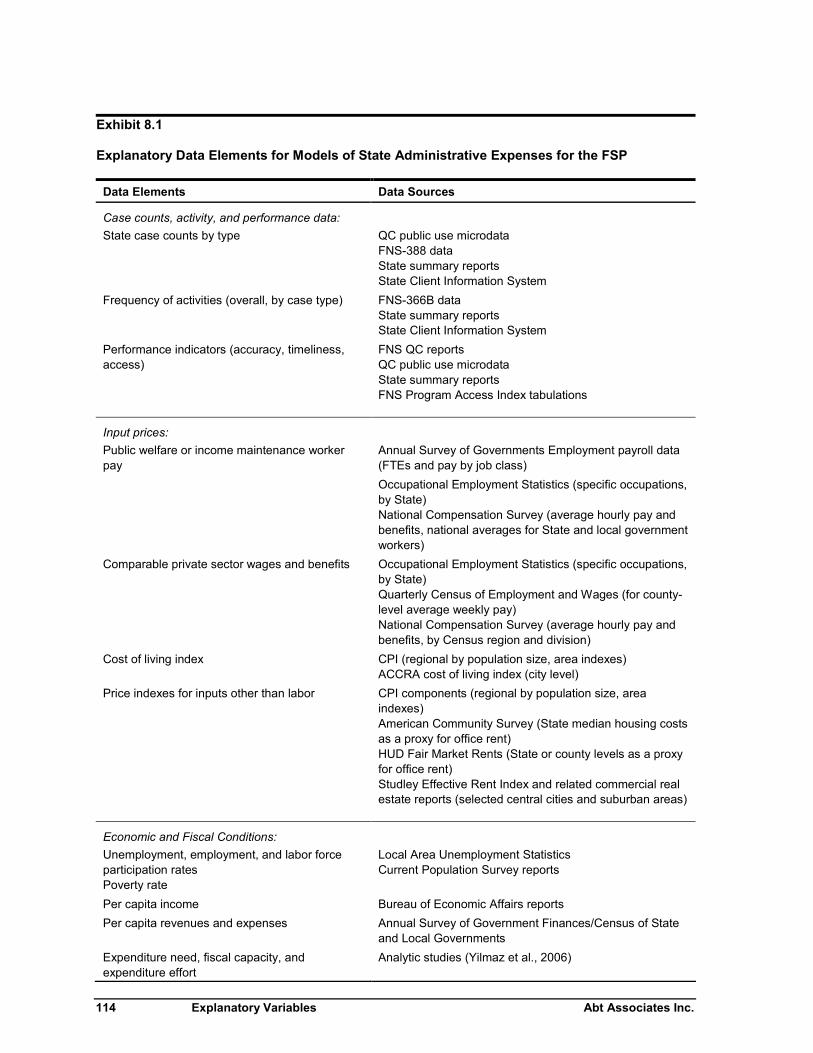
114 Explanatory Variables Abt Associates Inc.
Exhibit 8.1
Explanatory Data Elements for Models of State Administrative Expenses for the FSP
Data Elements Data Sources
Case counts, activity, and performance data:State case counts by type QC public use microdata
FNS-388 dataState summary reportsState Client Information System
Frequency of activities (overall, by case type) FNS-366B dataState summary reportsState Client Information System
Performance indicators (accuracy, timeliness,access)
FNS QC reportsQC public use microdataState summary reportsFNS Program Access Index tabulations
Input prices:Public welfare or income maintenance workerpay
Annual Survey of Governments Employment payroll data(FTEs and pay by job class)
Occupational Employment Statistics (specific occupations,by State)National Compensation Survey (average hourly pay andbenefits, national averages for State and local governmentworkers)
Comparable private sector wages and benefits Occupational Employment Statistics (specific occupations,by State)Quarterly Census of Employment and Wages (for county-level average weekly pay)National Compensation Survey (average hourly pay andbenefits, by Census region and division)
Cost of living index CPI (regional by population size, area indexes)ACCRA cost of living index (city level)
Price indexes for inputs other than labor CPI components (regional by population size, areaindexes)American Community Survey (State median housing costsas a proxy for office rent)HUD Fair Market Rents (State or county levels as a proxyfor office rent)Studley Effective Rent Index and related commercial realestate reports (selected central cities and suburban areas)
Economic and Fiscal Conditions:Unemployment, employment, and labor forceparticipation ratesPoverty rate
Local Area Unemployment StatisticsCurrent Population Survey reports
Per capita income Bureau of Economic Affairs reports
Per capita revenues and expenses Annual Survey of Government Finances/Census of Stateand Local Governments
Expenditure need, fiscal capacity, andexpenditure effort
Analytic studies (Yilmaz et al., 2006)
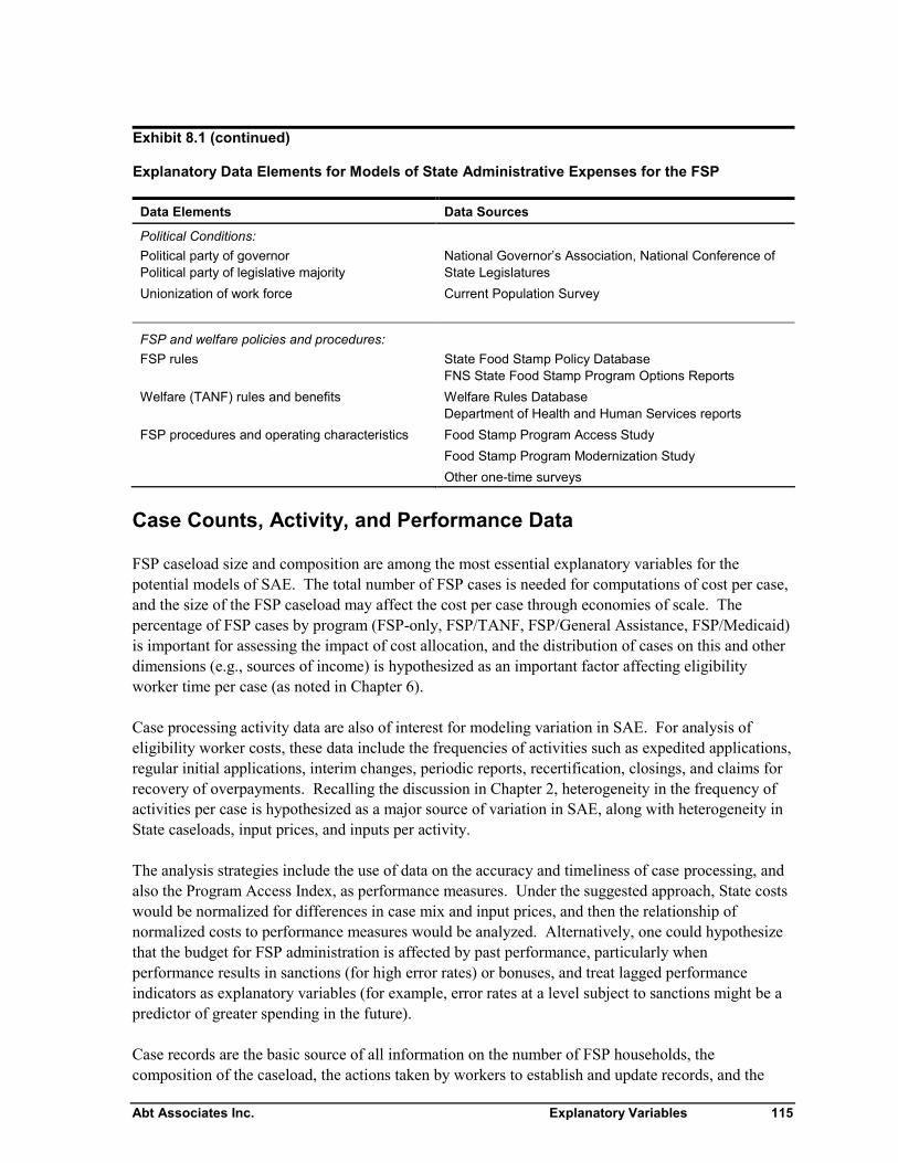
Abt Associates Inc. Explanatory Variables 115
Exhibit 8.1 (continued)
Explanatory Data Elements for Models of State Administrative Expenses for the FSP
Data Elements Data Sources
Political Conditions:Political party of governorPolitical party of legislative majority
National Governor’s Association, National Conference ofState Legislatures
Unionization of work force Current Population Survey
FSP and welfare policies and procedures:FSP rules State Food Stamp Policy Database
FNS State Food Stamp Program Options Reports
Welfare (TANF) rules and benefits Welfare Rules DatabaseDepartment of Health and Human Services reports
FSP procedures and operating characteristics Food Stamp Program Access Study
Food Stamp Program Modernization Study
Other one-time surveys
Case Counts, Activity, and Performance Data
FSP caseload size and composition are among the most essential explanatory variables for thepotential models of SAE. The total number of FSP cases is needed for computations of cost per case,and the size of the FSP caseload may affect the cost per case through economies of scale. Thepercentage of FSP cases by program (FSP-only, FSP/TANF, FSP/General Assistance, FSP/Medicaid)is important for assessing the impact of cost allocation, and the distribution of cases on this and otherdimensions (e.g., sources of income) is hypothesized as an important factor affecting eligibilityworker time per case (as noted in Chapter 6).
Case processing activity data are also of interest for modeling variation in SAE. For analysis ofeligibility worker costs, these data include the frequencies of activities such as expedited applications,regular initial applications, interim changes, periodic reports, recertification, closings, and claims forrecovery of overpayments. Recalling the discussion in Chapter 2, heterogeneity in the frequency ofactivities per case is hypothesized as a major source of variation in SAE, along with heterogeneity inState caseloads, input prices, and inputs per activity.
The analysis strategies include the use of data on the accuracy and timeliness of case processing, andalso the Program Access Index, as performance measures. Under the suggested approach, State costswould be normalized for differences in case mix and input prices, and then the relationship ofnormalized costs to performance measures would be analyzed. Alternatively, one could hypothesizethat the budget for FSP administration is affected by past performance, particularly whenperformance results in sanctions (for high error rates) or bonuses, and treat lagged performanceindicators as explanatory variables (for example, error rates at a level subject to sanctions might be apredictor of greater spending in the future).
Case records are the basic source of all information on the number of FSP households, thecomposition of the caseload, the actions taken by workers to establish and update records, and the
116 Explanatory Variables Abt Associates Inc.
accuracy and timeliness of decisions. Case data may be accessed in three basic forms: State clientinformation systems, the Quality Control sample file, and summary reports.
State Client Information Systems
When a household first applies for assistance, a record is created in the State client informationsystem (CIS). This record includes the information collected from the household and otherinformation from verification sources. The information is updated when the client provides newinformation (e.g., periodic reporting, change reporting, or recertification) or when new informationbecomes available from other sources, such as matching with employer wage reports. The caserecord includes demographic information on household members, income sources and amounts,deductible expenses, assets, and other information used to determine eligibility and benefits. To theextent that workers perform certification tasks through the CIS, there is a record of these tasks in thecase history, and there may be more detailed information in the “audit trail” of system usagemaintained as part of procedures assuring security and integrity of information systems. Thus, thereis a wealth of potential data for analysis of case composition and worker activities.
These records are regularly used for research under agreements with State Agencies, but there areburdens and challenges. Obtaining and using case record data requires access to documentation, thecapability to process files in the output format of the State system, and the cooperation of State staffto provide data extracts. Accumulating histories of cases or patterns of activity over time may requiremerging data from multiple extracts, each representing a month’s activity. CIS often have limitedhistorical data in the “production” databases at any time, so it may be necessary to process archivedata to obtain information for earlier periods. Thus, the most feasible use of case records is in cross-sectional analysis. Longitudinal analysis of case records over multiple years can represent a majorundertaking and cost for both the State and the contractor. Some States have established datawarehouses, however, which facilitate such analysis and can produce tabulations from datawarehouses upon request (UC Data, 1999). An updated study of such data warehouses and theircapabilities could be a useful foundation for future research.72
Quality Control Sample Public Use Microdata
The annual Quality Control (QC) sample comprises about 50,000 active food stamp cases selected forQC reviews. (About 40,000 cases with negative actions receive more limited QC reviews, but nocase characteristics are collected, and the data are not edited for analytic use.)73 Case records fromthe active case reviews are compiled by the States, submitted to FNS, edited, and made available inthe QC public use microdata files. Extensive data on household and participant characteristics areincluded (see Wolkwitz and Ewell, 2007). Of particular note, the QC data indicate when thehousehold was certified and when the next certification is due; thus, the data can be used to derive theproportion of cases subject to initial certification or recertification in each month. While QC data forsome years have an indicator for cases with interim actions, according to FNS these data areunreliable and are no longer included in the file. Each case record in these files indicates whether the
72 Ver Ploeg et al., 2001 provides general discussion on the uses of administrative data in studies of socialwelfare programs.
73 The purpose of the negative action review is to determine if the negative action (denial or termination ofbenefits) was done properly, not to determine if the household was ineligible. The data collection isdesigned to fulfill the specified purpose.
Abt Associates Inc. Explanatory Variables 117
QC review identified an underpayment or overpayment and the amount of the error. 74 Weights areprovided for estimates of population characteristics. National and State statistics on caseloadcharacteristics derived from the QC data are published annually (Wolkwitz, 2007). FNS producesannual estimates of State case and payment error rates for active cases and case error rates fornegative action cases. Starting in FY2003, FNS has used QC data to compute States’ rates of timelycase processing, and FNS awards performance bonuses to the six States with the highest percentagesof cases processed timely.
The QC microdata can be used to compute the distribution of FSP households by case type and Stateusing multiple dimensions. As the number of dimensions increases, the cell size and the precision ofthe estimates decreases. Thus, there is in principle a limit to how specific the case type categories canbe with acceptable precision for State-level estimates. In practice, our experience with these datasuggests that the precision of these estimates should be adequate. Appropriate analysis strategieswould define case types so that none was too small a percentage of the caseload. Based on apreliminary assessment, a minimum of 10 percent would be a reasonable threshold to assureacceptable precision for estimates of case mix percentages, but sampling error should be carefullyconsidered in the context of the exact use of the estimates.75 Case types representing less than 10percent of the caseload would not have much influence on the overall cost per case. Anotherlimitation is that QC procedures change from time to time, so there may be issues of non-comparability. Of particular note is the change in the threshold of countable errors from $5 to $25,starting in FY 2000. Thus, analysts must review documentation to assure that data elements arecomparable for the years being analyzed.76
Summary Reports
States are required to report to FNS on the number of participating households and individuals on amonthly basis, with a breakdown between public assistance and non-public assistance households (inthe FNS-388 report).77 These data when initially reported are estimates, so analysts must be sure touse final data. Households enrolled in Medicaid that do not receive cash benefits are not counted as
74 The original case records also identify cases that were determined ineligible in the QC reviews, althoughthese cases are excluded from the public-use data. Data on ineligible households is limited, because once areviewer identifies a household as ineligible, no further data are collected. Weights are provided forestimates of population characteristics from eligible cases.
75 With an average QC sample of 1000 per the State, a 10 percent population percentage would have aconfidence interval of around +/- 3%, including the design effect (Wolkwitz and Ewell, 2007). Smallergroups would have larger confidence intervals relative to the population percentage.
76 Another issue to be addressed is the existence of error in the household characteristics as determined byeligibility workers. For example, in identifying households with earnings, one could count only those withreported earnings, or one could also include those with unreported earnings identified in the QC review.QC records can be used to estimate the percentage with reported or unreported earnings, but thesepercentages would not be consistent with published statistics on FSP participant characteristics.
77 “Public assistance” includes TANF (cash and non-cash), GA, and State supplements forelderly/blind/disabled. Households enrolled in Medicaid that do not receive cash benefits are not countedas “public assistance” households.
118 Explanatory Variables Abt Associates Inc.
“public assistance” households. Thus, the full potential for cost-sharing among income maintenanceprograms cannot be determined from these data.78
States also report program activities on the FNS-366B report. Certification activity data includecounts of approvals, denials, terminations, and reinstatements; other activity counts are collectedregarding fair hearings, fraud investigations, disqualification hearings, and fraud prosecutions. TheFNS-366B report indicates the number of applications not processed within the required time, buttimeliness rates based on these data appear to be poorly correlated with timeliness rates computed in2003 and later on the basis of QC reviews (according to discussions with FNS headquarters personneland analysis presented in Logan, Kling and Rhodes, 2008). As discussed in Chapter 6, FNS-366Bdata are on a State fiscal year basis, so counts for Federal fiscal years will be based on averaging datafor two years and therefore will not fully reflect year-to-year changes.
Individual States also produce other summary reports for program management and accountability,including State summaries and breakdowns by county or local office. The States interviewed for thestudy had a variety of such reports, frequently available on their websites. The most common typewas a caseload report with counts of cases by program for each site, sometimes with counts ofworkers by site and total cases (across all programs) per worker as well. Two of the States hadinternal management reports that compared staffing to a weighted sum of cases across programs andcomputed a summary measure of worker caseloads versus a standard. Another type of report showedthe number of applications, recertifications, and closings by site. Also, State CIS generate reports ofsystem usage by program that may be used for cost allocation and for monitoring system usage.
While it appears to be impractical to collect a consistent set of such reports for a large number ofStates, they could be collected for a small number of States. This would be a way to obtain measuresof the frequency of certification activities at a lower cost than processing case records or QC data.Reports that break down data by office location could be analyzed to explore such questions aswhether differences in case mix by program have the same relationship to eligibility worker timeacross States and within States.
For analysis of the relationship of SAE to performance in the domain of program access, FNS reportson the Program Access Index (PAI) can be used. This measure is computed using administrative dataon the number of FSP participants and Current Population Survey data on the number of low-incomepersons (FNS, 2006). The PAI has been used since FY2003 to determine which States receivebonuses for the highest level of program access and the most improvement in program access. ThePAI methodology could be applied to earlier years. States often compute the ratio of food stampparticipants to Census estimates of persons in poverty at the county level as a measure of access; thisinformation could be useful in studying cost versus access where county-level costs are available (i.e.,where the FSP is county-administered, or where there is complete reporting of eligibility worker timerather than an RMTS).
78 Another potential issue with the FNS-388 data is the extent to which public assistance cases are definedconsistently. State TANF programs differ not only in cash benefit eligibility but also in eligibility for anduse of non-cash benefits, such as child care.
Abt Associates Inc. Explanatory Variables 119
Input Price Data
There are several kinds of input price data that might be appropriate for use in analyzing variation inSAE:
State data on actual pay rates for eligibility workers and other FSP workers (as discussed inChapter 6)
national surveys of public welfare worker pay national surveys of pay rates for comparable private-sector occupations general measures of price levels or the cost of living price indexes for other factors such as rent.
Variation in input prices across States is widely acknowledged and is expected to be a majoruncontrollable component of variation in SAE, so these data sources are very important. Asdiscussed in Chapters 4 and 6, data on eligibility worker pay and private-sector benchmarks wouldplay a critical role in separating the variation due to differences in eligibility worker time per case,market pay rates for eligibility workers, and actual eligibility worker pay. While Options 2, 3, 4, and5 assume the collection of actual pay rates for eligibility workers for one or more years, these optionswould require market pay rate data, and Option 1 would require an extant data source on pay rates forFSP workers or comparable private-sector workers. We discuss the national surveys and standardprice indexes below.
National Surveys of Public Welfare Worker Pay
There are two national databases that can be used to provide longitudinal data on pay rates forworkers in public welfare agencies in all States. First, the Census Bureau’s Annual Survey ofGovernments Employment (ASGE) provides annual payroll data by State, including number of full-time equivalents and total pay, for “public welfare workers”, a broad category that includes workersin income maintenance, social services, and other functions of public welfare agencies. These dataare based on surveys from all 50 States and a sample of local governments. Data for 1992 through1995 and 1997 through 2006 are currently available on-line,79 and data for 1989-1991 were providedfor the recent study of FSP certification costs and error rates (Logan, Kling, and Rhodes, 2008). Onelimitation of these data is that each State defines what is a “full-time equivalent” (FTE), based onstandard weekly work hours, but this definition is not specified. Thus, while the cost per FTE for twoStates could be the same, the cost per hour might be slightly different.
Second, the Occupational Employment Statistics (OES) program of the Bureau of Labor Statisticsprovides average hourly wage rates by State for specific occupations, including “eligibilityinterviewers”, i.e., “eligibility workers” as defined in this memorandum (BLS, 2008a). OESoccupational wage averages by State for 1999-2006 are available on-line; 1997 and 1998 data also areavailable from the Bureau of Labor Statistics (BLS). The OES data are more specific, but the ASGEdata reflect the actual mix of “public welfare workers” in different occupations. The choice betweenthese sources would depend on the specifics of the analysis, and both sources could be used inimplementing Option 1.
79 The ASGE was not conducted in 1996 (Census Bureau, 2008a).
120 Explanatory Variables Abt Associates Inc.
Comparable Pay for Private Sector Workers
As we have argued in Chapter 3, a market wage indicator is a better measure of pay than the actualFSP worker pay if the intention is to represent the uncontrollable variation from State to State. Thedifference between actual and market pay reflects State or local decisions. The OES data provideaverage wages by State for over 800 occupations. The “eligibility interviewer” occupation fallswithin the major occupational group of “office and administrative support occupations”. The overallaverage for this group could be used as a market pay index, or more specific occupational informationcould be used.
The choice of the market “benchmark” could have an effect on the analysis, although the variety ofdata would make a sensitivity analysis possible (indeed desirable). While the benchmark occupationor occupation group should be reasonably comparable to eligibility workers in terms of qualificationsand duties, the match does not have to be exact. The benchmark pay rate will be used to create anindex of the State’s market pay level relative to the national average. Thus, what is most important isthat the differences among States in pay for the benchmark occupation provide good estimates of thedifferences in eligibility worker pay that one would expect if States hired similar workers under thesame conditions as private employers.
To benchmark county-level pay for eligibility workers or other FSP workers for analyses of costdifferences among counties, the county-level average weekly pay statistics from the Quarterly Censusof Employment and Wages (QCEW) could be used. These data are obtained by State unemploymentagencies from all employers covered by unemployment insurance, and county-level averages areavailable from BLS for 1990 and later (BLS, 2008d). These data are less comparable across locationsand over time than the OES data because they are weekly averages; thus, they reflect variation in paidhours per week as well as in hourly pay rates. In addition, the QCEW weekly average pay includesbonuses, overtime, and other compensation in addition to regular pay. Therefore, although Stateaverages are available from the QCEW, the OES data are preferable for the anticipated uses in thiscontext. As discussed below, the OES data are also preferable to other sources of market pay rates.
Analysts may wish to benchmark benefits or total compensation for FSP workers to private sectoraverages, either overall or for specific industries or occupations. The National Compensation Survey(NCS) collects data on pay and benefits by occupation from a national sample of establishments(BLS, 2008c). Data have been collected from both public and private employers since 1991.Published reports from the Employer Cost for Employee Compensation (ECEC) program provideannual averages of pay and benefit cost per hour for private employers by occupation, separately byCensus region and division, and by metropolitan versus nonmetropolitan location. However, thepublished reports provide only national averages for state and local government employees, by broadoccupational categories that are much less specific than the ASGE or the OES. Thus, these data aremore useful for establishing private sector benchmarks than for independently estimating average payand benefits for public welfare workers. Furthermore, they do not provide State-level estimates forany industries or occupations. Analysis of the available data and related literature might be used todetermine how important the lack of State-level data would be for explaining variation in totalcompensation.
Abt Associates Inc. Explanatory Variables 121
General Price or Cost of Living Indexes
As an alternative to wage data, a general price or cost of living index could be used to estimate theeffects of market input price differences on total SAE. This approach has some appeal for models oftotal SAE, which includes both labor and nonlabor costs. The key limitation of price and cost ofliving indexes in this application is that they measure variation in a basket of goods and services thata typical household would buy, whereas SAE comprises a very different mix. Given the expectationthat most of SAE is for labor, wage measures may be preferable. On the other hand, a general priceor cost of living index might be considered a reasonable variable to use in analyzing variation inoverhead (which includes labor and non-labor costs) or in a pool of varied non-labor costs. Thechoice of variables depends on the analysis, and alternative approaches can be tested and compared insensitivity analysis.
The primary measure of general price variation across the nation is the Consumer Price Index (CPI).This index is computed monthly for the four Census Regions cross-classified by size of city, and for27 metropolitan areas. It is not computed for individual States, but regional or metropolitan areaindexes could be used (BLS, 2008d).
Another general price index is the ACCRA Cost of Living Index, published by the Council forCommunity Economic Research (C2ER). This index has been produced annually since 1980 at thecity level, using price data for representative goods and services and weights based on the ConsumerExpenditure Survey (C2ER, 2008). Population data at the city level within State could be used tocompute a State-level index.
Price Indexes for Inputs Other than Labor
While the options defined in Chapter 4 focus on analysis of variation in pay, the prices of other inputsmight be useful for analyzing variation in FSP SAE. The other inputs include supplies, equipment,data processing and telecommunications services, and facilities.80 One possible source of data oninput prices is the Consumer Price Index, which has indexes for specific categories of goods andservices, such as housing. Differences in consumer costs for housing could be used as a proxy forvariation in commercial rents, under the assumption that the markets are related and driven by thesame underlying economic forces. This assumption does not take into account the differencesbetween commercial and residential housing markets, such as the different cycles of demand andsupply, but it may provide a reasonable proxy for differences in facility costs among States. As withthe overall CPI, component indexes are not available at the State level, but the available geographicdetail would allow some control for regional differences.
We have searched for but not identified a public State-level index for commercial real estate.Proprietary research firms offer indices based on rent or property values for major market areas; thesemarkets are not necessarily representative of statewide averages. Most notably, the Studley EffectiveRent Index provides comparisons of effective commercial rents for 16 top central city markets and 16top suburban markets; this data series extends back to 1995 (Studley, 2008). Studley also offers
80 The cost of facilities includes utilities, maintenance, and rent or depreciation of buildings and fixtures.Given the varied ways in which these costs might be paid, comparisons across States would be best madeon the basis of the total cost of facilities, for which a measure of gross rent would be a suitable proxy.
122 Explanatory Variables Abt Associates Inc.
reports of total rent per square foot averages for 18 major markets and 50 secondary markets.81 Wehave identified several indexes of commercial property values, but none with State-level values oreven coverage of the largest city in each State. As an example, Real Capital Analytics, maintains adatabase of all commercial property sales over $2.5 million starting in 2001 (RCA, 2008); thisdatabase is used to compile an index of commercial real estate prices for four regions of the nationand selected metropolitan areas. While indexes of property values for States are feasible according toone source, this has not been done except on a test basis in Florida (Gatzlaff and Holmes, 2007). Akey issue for property indexes based on transaction prices is that sales within markets may beinfrequent and heterogeneous, making indexes volatile. A deeper issue is that an index of currentproperty values does not reflect the cost of properties when acquired by a State five, ten, or moreyears in the past.
In the absence of indexes for commercial property costs, an index of housing costs might be used as aproxy for the relevant economic conditions. For facilities, there are two sources of housing costcomparisons that could be used to construct indexes of differences in costs across States and overtime. The 2000 Census and the American Community Survey (ACS) provide State level estimates ofmedian monthly housing costs for renters, including rent and utilities. ACS estimates are availablefor 2002 through 2006 (Census Bureau, 2008b). Another approach would be to use Fair MarketRents computed by the Department of Housing and Urban Development (HUD). HUD computes FairMarket Rents for 530 metropolitan areas and 2,045 nonmetropolitan county FMR areas, based on areaCensus gross rent data updated using regional data from the American Housing Survey or HUDsurvey data (HUD, 2008).82 While the Fair Market Rents data allow comparisons within a State, thevalidity of these data as a basis for comparing office costs is questionable. Given the uncertaintiesabout separating rent or depreciation from other nonlabor costs (as discussed in Chapter 7) and thelimitations of the available indexes, it appears that the most practical way to adjust nonlabor costs foruncontrollable price differences is to use a general cost of living index, i.e., the CPI or the ACCRAcost of living index.
General Environment
Analysis of variations in FSP SAE may seek to take into account the general environment in whichStates operate. These types of variables include economic, fiscal, political, and social conditions.These variables may affect SAE, performance, or both; they are particularly important for analysis ofvariation in activity rates and for comparisons of normalized costs to performance measures. Thespecific variables of interest would depend on the dependent variable (total SAE per case, eligibilityworker time per case, eligibility worker time per task, etc.) and the hypotheses for the model. Belowwe summarize standard data sources in this general category.
81 Effective rent is the preferable measure; it takes into account total rent and the terms of the lease,particularly concessions (e.g., if the first three months are free).
82 The American Housing Survey produced biannual reports on a national basis and estimates for selectedmetropolitan areas every 6 years (Census, 2008c). Thus, this survey would not be useful for studies ofvariation in SAE.
Abt Associates Inc. Explanatory Variables 123
Economic Conditions
The measures of State economic conditions for modeling SAE include: rates of employment,unemployment, and labor force participation; poverty rates; and per capita income. Trends in thesevariables may also be hypothesized to affect the amount of work required to administer the FSP. Forexample, Hamilton et al. (1989) found that the eligibility worker time per case rose with theunemployment rate and the rate of change in the unemployment rate, because volatility inemployment produces volatility in the eligibility and benefits of FSP households. Economicconditions that affect the FSP caseload might be used in a model in place of the actual FSP caseload,in order to separate the effects of caseload characteristics from those of policies that affect SAE andFSP participation. The Current Population Survey provides monthly State data on employmentstatistics and annual data on income and poverty. An alternative source for employment statistics isthe Local Area Unemployment Statistics (LAUS) program (BLS, 2008e), which is a joint program ofthe BLS and the State workforce agencies. Annual State income and poverty data are also availablefrom the American Community Survey. The Bureau of Economic Affairs produces annual Statestatistics on per capita income and State GDP (BEA, 2008).
State Fiscal Conditions
Possible measures of State fiscal conditions include per capita revenues, per capita expenditures,fiscal capacity, and revenue effort. As discussed in Chapter 2, we hypothesize that a State’s FSPbudget is affected by its overall fiscal capacity and the competing demands for funding. Budgetconstraints may affect the frequency of tasks, the eligibility worker time per task, and the quality oftask performance. With the exception of fiscal capacity, fiscal conditions are controllables from theperspective of State government as a whole, but they are arguably uncontrollables from theperspective of FSP managers. Annual data on State revenues and expenditures are available from theAnnual Survey of Government Finances, conducted by the Census Bureau (Census, 2008d). Thesame data are collected every five years in the Census of State and Local Governments.
Fiscal capacity and revenue effort are analytic constructs derived from fiscal data and Statecharacteristics. Fiscal capacity is the ratio of potential revenue to “need” for spending; these twoquantities are estimated using models of the relationships of State characteristics to revenues andexpenditures. Potential revenue, need for spending, and fiscal capacity are intended to be objectivemeasures that are independent of the actual revenue and spending choices of the State. Revenueeffort is the ratio of actual revenue to potential revenue; this reflects State choices. State indexes forthese variables have been estimated for 2002 and earlier years (Yilmaz et al., 2006).83 While themethodology could be replicated for other years, this would appear to be a major undertaking.Therefore, these variables could not be used in a time-series model with State fixed effects, but theycould be used to analyze the State fixed effects in an additional step. They also could be used incross-sectional analysis, such as the analysis of task frequency and the State-specific intensitymeasure for any version of Option 5.
83 Yilmaz et al. (2006) reference prior reports using similar methods for 1991, 1997, and 1999.
124 Explanatory Variables Abt Associates Inc.
Political Conditions
In the conceptual model in Chapter 2, the political preferences of a State’s electorate directly affect itsFSP budget and its policies, and indirectly affect FSP management. Conventional indicators of Statepolitical conditions in the literature on FSP participation (e.g., Kabbani and Wilde, 2003) include thepolitical party of the governor and the party controlling one or both houses of the legislature. Thesedata are available from the National Governor’s Association and the National Conference of StateLegislature. The party of the Presidential candidate winning the State in the most recent election isanother indicator, but it is not annual. Lastly, the AFDC/TANF benefit level for a standard familyunit is often used as an indicator of the State’s propensity to spend on assistance to low-incomehouseholds; this information is available from reports published by the Administration for Childrenand Families, Department of Health and Human Services (e.g., HHS, 2006) and also from theWelfare Rules Database (discussed below).
The degree of unionization of a State’s work force may be a factor affecting pay rates for eligibilityworkers and other personnel; this variable might also be a good indicator for more general politicalpreferences affecting the FSP budget, policies, and management. The BLS reports annually on unionmembership and representation of workers by State and the national median pay for union versusnon-union workers (BLS, 2008e). The reported State-level data do not indicate the percentage ofunionized workers in public versus private employment. Pay differentials also are not reported at theState level. Union membership data from the CPS might be tabulated across multiple years toestimate average unionization rates for public versus private employees by State. It may also bepossible to use CPS microdata for this analysis.
Social Conditions
In the conceptual model, characteristics of the State low-income population affect the size of the FSPcaseload, the case mix (percentage of households by type), and the share of common costs formultiple programs allocated to the FSP. (The size of the low-income population and the poverty rateare included in the variables for economic conditions listed above.) The population interacting withthe FSP includes households that inquire about FSP but do not apply, and those that apply and aredenied food stamp benefits, as well as participants. Possibly relevant dimensions include age,immigration status, mobility, and population density. Using general low-income populationcharacteristics rather than FSP participant characteristics would control for the possible effects ofspecific policies on differential participation by demographic groups (e.g., simplified applications oroutreach for senior citizens).84 A wide variety of social indicators at the State level are available fromthe Census, CPS, and American Community Survey, and for other Federal statistical programs.
84 One might attempt to model the effects of fiscal conditions in a reduced form approach by including factorsaffecting the demand for social welfare spending in general, such as dropout rates, crime rates, and teenpregnancy rates. In the literature on fiscal capacity and expenditure effort, the models of these fiscalconditions are complex. Therefore, we believe it is preferable to keep these models separate and use theirresults, rather than use the reduced form approach.
Abt Associates Inc. Explanatory Variables 125
Characteristics of State FSP Operations
There are several available sources on specific aspects of FSP operations. As discussed below, somenational sources are longitudinal, while others are intermittent or one-time products.
FSP Policy Variables Databases
For potential studies of policy impacts on SAE, the State Food Stamp Policy Database is an importantresource. This longitudinal database of State Food Stamp policies was compiled for a recent study ofFSP participation (for description and documentation, see Finegold et al., 2008). Covering 1996through 2004, the database includes measures of State FSP policy options regarding certificationperiods, reporting requirements, categorical eligibility, transitional benefits, immigrant eligibility, andvehicle exemptions. Selected data are currently being updated to add values for 2005. Data for morerecent years on many variables in this database are available from FNS’ annual State policy optionsreports (such as FNS, 2006b).
For older time periods, data on State policies might be obtained from FNS’ database of waivers toFSP regulations (FNS, 2008c). Using this database would be challenging and potentially time-consuming, however, for two reasons. First, the database captures the specific details of waivers,which vary among States even when the basic purpose of the waiver is the same. For quantitativeanalysis, the similar waivers would have to be grouped. Second, waivers granted by FNS may nothave been fully implemented by the States.
For some policies, additional data may be needed to analyze their cost impacts. For example, theState Food Stamp Policy Database identifies States with expanded categorical eligibility for the FSP,including households receiving TANF services but no cash assistance. Potentially relevant detailsmight differ among States: what types of services would qualify a household, and what proportion ofFSP households is approved on this basis. The latter question can be answered by analyzing the QCmicrodata, but new data may be required if there is a desire to analyze the impacts of policy detailssuch as the proportion of cases assigned to simplified reporting.
We have noted previously the limited degrees of freedom available, even when analyzing nine ormore years of 50-State time series data. Thus, the number of policies that can be included in feasiblemodels is finite, even when costs are normalized and degrees of freedom are not needed for suchfactors as case mix and economic conditions. For more detailed policy variations, an alternativeapproach is to collect and analyze detailed data on the costs of specific tasks affected by the policiesmay be the most effective approach; this was the method used for estimating the impact of changingfrom coupon to EBT issuance on eligibility worker and clerk costs (e.g., Logan et al., 1994).
Welfare Rules Database
TANF rules may be another area of interest for analysis of SAE. For example, TANF policies todivert applicants may alter the flow of applicants so that TANF income eligibility determinationoccurs after a household has already been approved for food stamps. As a result, the FSP may bearmore of the costs of joint eligibility determination activities than when the full TANF application isprocessed at the same time as the food stamp application. TANF policies could also contribute tomore or less frequent changes in food stamp cases, particularly when food stamp sanctions are linkedto TANF sanctions. The influence of TANF policies has diminished as the proportion of FSP
126 Explanatory Variables Abt Associates Inc.
households receiving TANF has dropped: in FY2006, only 13 percent of FSP households receivedTANF (Wolkwitz, 2007).
The Welfare Rules Database, created and maintained by the Urban Institute, provides longitudinaldata on State TANF rules from 1996 through 2003 (Rowe and Versteeg, 2005). This databaseincludes four main categories of rules: initial eligibility, benefits, work and other requirements tomaintain benefits, and ongoing eligibility (including family caps and time limits). The data areaccessible through a series of reports and an online database.
Surveys of State FSP Operations
Data on State FSP operations may be obtained from existing or new surveys of State and localagencies. Such surveys would have to be done regularly to compile a longitudinal database, and thiswould represent a considerable expense. Thus, primary data collection is more feasible and generallyhas been done on a one-time basis.
Several surveys have collected data on State FSP operations; two such surveys are of particularinterest for studies of certification costs. First, the Food Stamp Program Access Study collected dataon State and local policies and procedures expected to affect access to the FSP (Bartlett et al., 2004).Public-use data from the State and local agency surveys are available. Second, the FSPModernization Study collected extensive data in 2007 on State efforts to improve the efficiency,accuracy, and accessibility of certification and other operations. Topic areas included: organization,administration, technology, partnering with community organizations, alternative interfaces withcustomers (call centers, electronic applications), biometric identification technology, and outreach.The data on organization and programs administered closely align with characteristics hypothesizedto affect long-term cost differences among States. Data on the role of community partners from theModernization Study could be important, since these partners may assist in the application process atlittle or no cost to the FSP. For each of these areas, questions included the timing and scope of thechanges, the State’s objectives, and outcomes. Such a survey provides a wealth of information that isboth a boon and a challenge. From a qualitative perspective, this information can be used tounderstand similarities and differences in modernization efforts across States. For quantitativeanalysis, the large number of variables poses a challenge for specifying models that can be estimated(due to the potential for insufficient degrees of freedom or collinearity). Thus, for such data to beuseful in explaining cost differences among States, the data would have to be analyzed and “boileddown” to the major differences among States.
Interviews with State officials for this study point to an important caution about collectinginformation on how the FSP operates at the local level. State officials may be familiar with thepossible variations of structure, such as whether some offices have separate intake and ongoing caseunits, and variations in client flow (such as use of support staff to collect application information).However, State officials may not know how often the variations in structure or client flow actuallyoccur, or whether there is a “typical” configuration for a local office. When these decisions aredelegated to local managers, States may not have the resources or the need to track them. As a result,surveys that seek to establish the standard or typical practices will be more reliable if they collect dataat the local office level, except in the States with the most top-down approach to managing localoperations.
Abt Associates Inc. Explanatory Variables 127
Summary
The preceding discussion makes clear that there is a wealth of data that can be used to analyzevariation in SAE. In particular, there are strong national databases with State-level time series dataon the following types of explanatory variables:
case counts and characteristics frequency of certification and recertification, by case type pay for public welfare workers and comparable private sector occupations economic conditions State revenues and expenditures political and social conditions FSP and welfare rules.
There are, however, some important limitations and challenges.
Other than the public assistance/non-public assistance breakdown in FNS data, analysts mustobtain State reports, or else they must process QC microdata or State client data to determinethe proportion of food stamp cases of different types.
State client data must be processed to determine the frequency of activities that are notreported in the FNS-366B or to determine the frequency of activities by case type (other thancertification and recertification, which can be identified in QC microdata).
While wage rates are available at the State level, benchmarks for benefits are available onlyat the regional level, and union/non-union wage differentials are available only nationally andfor specific metropolitan areas.
There are no State-level benchmarks or indices for the costs of resources other than laborused in FSP State and local operations. For rent/depreciation of facilities, variations inhousing costs by State or metropolitan area office rents could be used, but these sources haveimportant limitations. In general, it appears that the most practical strategy for normalizingnonlabor costs is to use the regional CPI or the ACCRA index as a proxy.
Expenditure need, fiscal capacity, and expenditure effort are interesting concepts but requireconsiderable effort to replicate the existing methodology.
Longitudinal databases of FSP and welfare rules are available, but they are extensive anddetailed, and require analysis to construct summary measures for analysis of SAE.
FSP procedures and operating characteristics are not documented on an ongoing basis,although some one-time surveys are available. As operating procedures become more diversethrough use of technology and different business processes, this information will becomemore important.

128 Explanatory Variables Abt Associates Inc.
Abt Associates Inc. Conclusions and Recommendations 129
PART III: CONCLUSIONS AND RECOMMENDATIONS
This part of the report presents the conclusions regarding the study questions, compares the feasibilityof the study options, and describes a suggested program of research on SAE.
Chapter 9
Conclusions and Recommendations
This report has assessed the potential approaches, data requirements and sources, and overallfeasibility of explaining variation in State administrative expenses (SAE) for the FSP. Two sets ofquestions were posed in Chapter 1:
Is it possible to measure food stamp administrative expenses consistently enough acrossStates to credibly assess the degree of variation? If it is possible, what are the alternativeways to measure such expenses? Are new data required? If so, what level of effort would berequired and what challenges would need to be addressed to obtain such data?
How well can variation in State food stamp administrative costs be explained with non-experimental methods? What are the alternative approaches, and what are the advantages anddisadvantages of each? Which approach is recommended and why?
In addition, we have considered the potential sources for variables to explain the variation in SAE. Inthis chapter, we summarize our answers to these questions and outline a program of potential studiesof variation in SAE. Our recommendations take into account the interactions of data and analysisstrategies, and the implications for the most feasible analytic approaches.
As discussed in Chapter 1, we have assumed that the primary interest is in the variation incertification costs, and we have argued that variation in the costs of other client service functionsshould be studied separately. The discussion of data sources has focused, accordingly, onmeasurement of certification costs, with attention to automated data processing (ADP) costs as asecondary interest. We also have addressed, in less detail, the potential data sources and issues forstudying the costs of other functions, including nutrition education, issuance, and employment andtraining.
Feasibility of Obtaining Consistent Measures of SAE
In general, there appears to be sufficient consistency in the reporting of SAE for the FSP to permitvalid comparisons across States and over time. This conclusion applies to all components of SAE.This consistency is due to the extensive controls at the State and Federal levels to assure that claimsfor reimbursement are accurate and that the allocation of costs across programs is equitable.
There are some important qualifications to this conclusion with respect to certification and ADPcosts.
130 Conclusions and Recommendations Abt Associates Inc.
The “certification” reporting category does not provide a consistent measure across States,but this problem can be solved by creating an analytic measure that also includes the“unspecified other”, “reinvestment”, and “outreach” categories. A broader measure thatincludes related activities may be desirable for analyses relating certification costs toeffectiveness.
There is substantial uncertainty about how to compare ADP costs across States and over time.These costs should be studied separately, taking into account specific information about ADPsystems, before attempting to relate ADP costs to certification costs.
There is some risk that local costs are less accurately reported when States use personnelactivity reports instead of RMTS for multi-program staff.
Comparisons of State-level management and oversight costs might be affected by differencesin cost allocation methods, but these costs are a relatively small portion of SAE.
Changes in cost allocation rules must be taken into account in comparing certification costsprior to 1999 with later years. It is possible to make adjustments for these changes, but theseadjustments would complicate the modeling of changes in these costs over time.
Because of time lags in the reporting of SAE, comparisons will be most valid when based onfinal annual expenses. For States where counties administer the FSP, reporting lags mayaffect comparisons of expenses with other States and with trends in explanatory variables.
A study of SAE would be strengthened by collecting some simple items of information fromStates about the methods used to allocate time for multi-program eligibility workers and othershared costs at the local level, and in central units performing certification functions.
Detailed Cost Data Desirable to Explain Variation
We may seek to explain variation in SAE in two different ways. First, we may seek to determine howmuch of the overall variation can be explained by factors that States cannot control (such asprevailing wages, and demographic and economic conditions) and by factors that States can control(such as policies, management decisions, and investments in computer technology). The moreinterstate variation in FSP SAE is due to controllables, the larger is the scope for cost savings.Second, we may seek to determine the difference in SAE attributable to specific policies, such assimplified reporting, or specific management practices, such as use of call centers to process casechanges.
Conceptual Framework for Defining Data Needs
In this report, we have presented a conceptual framework for analyzing SAE at the input level (e.g.,labor costs), the case level (i.e., cost per case by type of case), and the task level. We have definedthe ideal data on SAE as comprising the quantities of inputs used and the FSP share of that usage foreach task for each type of case, the frequencies of tasks by type of case, the distribution of cases bytype, and the market prices of inputs. The ideal data cannot be obtained in practice, but we haveenvisioned simplified approaches that will enable us to understand the sources of variation in SAE.
This framework makes clear that it is highly desirable to disaggregate SAE as much as practical alongthe dimensions of the ideal task level framework. While a conventional regression analysis ofaggregate SAE at the State level could certainly be undertaken, and indeed is one of the
Abt Associates Inc. Conclusions and Recommendations 131
recommended approaches, it would have two important limitations. First, with a large number ofpossible explanatory factors, we are likely to run out of degrees of freedom to estimate effects withconfidence. Second, a linear specification with variables having additive effects appears to be a poorapproximation of the true model.
To disaggregate SAE along the lines of the conceptual framework, we would need some or all of thefollowing kinds of cost data, in addition to aggregate SAE per case by State and year:
breakdown of SAE among inputs, particularly between eligibility workers and other inputs prices and quantities of inputs, particularly eligibility worker time and pay distribution of eligibility worker time by type of case frequency of eligibility worker tasks and time per task
We focus on eligibility worker labor as the input of greatest interest because these workers play thelargest role in the usual certification process.
The specific data requirements and the feasibility of meeting those requirements depend on theapproach to disaggregating SAE. We have identified five feasible options for explaining the variationin SAE using extant or new cost data at varying levels of aggregation. The five options and their datarequirements are summarized in Exhibit 9.1 (repeated from Exhibit 4.2). One option (Option 1)would model aggregate State-level SAE per case (specifically, certification costs) as reported byStates to FNS. These cost data are certainly available.
The other four options would implement different parts of the ideal disaggregation of SAE. Option 2would break down total certification costs into three key variables: eligibility worker hours,eligibility worker pay per hour, and the “generalized overhead rate”, defined as the ratio of all othercosts to eligibility worker costs. This option would require data from State financial records. Options3 and 4 would further break down the eligibility worker hours by case type; Option 3 would do thisfor all States, while Option 4 would do this in a sample of States and use the data to construct adifficulty index of the relative effort for each type of case. These options would thus require data onthe distribution of eligibility worker time by type of case. Option 5 would break down the eligibilityworker hours at the task level as a function of time per task and task frequency by case type. Option5 could be implemented with the Option 2 cost data alone or with State-level data on the averageeligibility worker time per task; all versions of Option 5 would use State-level data on the frequencyof tasks by case type. Under all of these options, additional State-level data would be needed to breakdown the overhead rate into components for separate analysis (labor vs. non-labor, local vs. State,etc.).
In the discussion that follows, we focus on the feasibility of collecting valid, comparable cost datafrom existing or new sources to meet the requirements of the options. The conclusions on theavailability of the explanatory variables are presented in the next section. Following that discussion,we summarize the strengths and weaknesses of these options for analysis of variation in SAE.
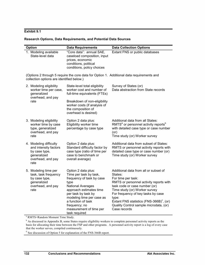
132 Conclusions and Recommendations Abt Associates Inc.
Exhibit 9.1
Research Options, Data Requirements, and Potential Data Sources
Option Data Requirements Data Collection Options1. Modeling available
State-level data“Core data”: annual SAE,caseload composition, inputprices, economicconditions, politicalconditions, policy choices
Extant FNS or public databases
(Options 2 through 5 require the core data for Option 1. Additional data requirements andcollection options are identified below.)
2. Modeling eligibilityworker time per case,generalizedoverhead, and payrate
State-level total eligibilityworker cost and number offull-time equivalents (FTEs)
Breakdown of non-eligibilityworker costs (if analysis ofthe composition ofoverhead is desired)
Survey of States (or)Data abstraction from State records
3. Modeling eligibilityworker time by casetype, generalizedoverhead, and payrate
Option 2 data plus:Eligibility worker timepercentage by case type
Additional data from all States:RMTSa or personnel activity reportsb
with detailed case type or case number(or)Time study (or) Worker survey
4. Modeling difficultyand intensity factorsby case type,generalizedoverhead, and payrate
Option 2 data plus:Standard difficulty factor bycase type (ratio of time percase to benchmark oroverall average)
Additional data from subset of States:RMTS or personnel activity reports withdetailed case type or case number (or)Time study (or) Worker survey
5. Modeling time pertask, task frequencyby case type,generalizedoverhead, and payrate
Option 2 data plus:Time per task by task,frequency of task by casetypeNational Averagesapproach estimates timeper task by task bymodeling time per case asa function of taskfrequency; nomeasurement of time pertask required
Additional data from all or subset ofStates:For time per task:RMTS or personnel activity reports withtask code or case number (or)Time study (or) Worker surveyFor frequency of key tasks by casetype:Extant FNS statistics (FNS-366B)c, (or)Quality Control sample microdata, (or)Case records
a RMTS=Random Moment Time Study.b As discussed in Appendix B, some States require eligibility workers to complete personnel activity reports as thebasis for allocating their time between the FSP and other programs. A personnel activity report is a log of every casethat the worker serves, compiled continuously.c See discussion of Option 5 for explanation of the FNS-366B report.
Abt Associates Inc. Conclusions and Recommendations 133
Feasibility of Obtaining Data for Options 2, 3, 4 and 5
Of the four options for analyzing eligibility worker time, pay, and “overhead”, Option 2 is clearly themost feasible, because the data requirements are much more modest. The version of Option 5 basedon national average time per task is also more feasible than the other options. There are, however,several key caveats about Option 2; these also caveats apply to Options 3, 4, and 5, which require thedata for Option 2 as a starting point.
There is uncertainty about whether a consistent definition of “eligibility worker” can beapplied to collect comparable data on eligibility worker costs and “overhead” from existingsources in all States. Information from States via a survey would be helpful to resolve thisuncertainty. Using total local office labor instead is potentially an acceptable fall-back, butthis would complicate the comparisons of pay and benefits.
Data on eligibility worker time, pay rates, and benefits from State records could be collectedfrom most States with relatively modest effort and burden on States, but the effort and burdento assure that these estimates are entirely comparable could be substantially greater.
Option 2 would be more complicated, costly and burdensome in county-administered Statesand where some eligibility worker functions are performed in call centers, but we do notanticipate that it would be infeasible to include such States in a study based on Option 2.
Analysis of the labor component of overhead appears to be feasible, as is breaking downoverhead by agency level (local, State program administration, statewide). Breaking outspecific types (objects) of nonlabor costs is likely to be challenging. The feasibility ofcomputing desired summaries from the detailed data in accounting systems depends on thecapabilities of the accounting system, how FSP is computed, and the cooperation of Stateofficials.
Decentralized accounting data pose challenges and opportunities for collecting data on thecomposition of overhead where counties operate the FSP under State supervision.
A limited version of Option 3 appears feasible to implement on a national scale: collecting existingdata on the percentage distribution of eligibility worker time by program combination (FS-only, FSand Medicaid, etc.). This information exists in States that conduct that administer programs jointlyand collect this information for cost allocation purposes through random-moment time studies(RMTS) or activity reports. These existing data are feasible to collect and would be informative, butthe combination of programs is only one of the case type dimensions of interest. We would also likeinformation on relative effort required for other case characteristics that are likely to shift SAE percase. Those case characteristics are likely to include whether the case has earnings, the number ofindividuals in the case, and whether the case includes elderly persons. New data collection would bepossible, but would be very expensive, and would only provide a cross-section as of the time in whichthe new data were collected (rather than a time series of data for each State spanning several years).
Option 4 simplifies the data requirements of Option 3 by assuming that the relative difficulty of eachcase type does not vary systematically by State, so data on eligibility worker time by case type from asmall number of States can be extrapolated to all States and all time periods using available aggregatedata on case mix (e.g., QC data or FNS Form 366B data). While this assumption may not be strictlycorrect, it provides a basis for feasible and potentially insightful analysis. To implement Option 4,
134 Conclusions and Recommendations Abt Associates Inc.
there are three potential designs, listed below in order of increasing richness of data, cost, and burden,with their chief challenges:
Collect existing data from States that identify case type in their RMTS or activityreports. This approach would only be viable if a sufficiently representative group of Stateshad comparable data.
Merge case records with existing RMTS or activity report data to estimate theproportion of time by case type. Issues for this option include: uncertainty about how manyStates have case identifiers in their time use data, and potential logistical and privacy issues ifthe researchers have to process original hard-copy time reporting forms in order to obtain thetime data with case identifiers. The effort to acquire and process case records would makethis approach infeasible for Option 3 but it appears feasible in a small number of States forOption 4.
Collect new time-use data from eligibility workers in a sample of offices within theselected States and match these data to case records. Such a study could provide data ontime by task as well as by case type; thus it would be a combination of Options 4 and 5. Thisapproach was used in the FSP certification cost study. A full replication of the prior studywould be very expensive and burdensome, but would yield very rich data. A smaller-scaleversion designed only to estimate overall time per task would be more feasible. A keychallenge for such a study is assuring that the sample of offices provides sufficientlyrepresentative data for national estimates (and State estimates if desired). New time-use datawould be limited to the period for which they were collected, whereas extant data would beavailable for three to five years.
There are three versions of Option 5 that appear to be feasible. All three versions could use existingnational databases providing the aggregate frequency of major tasks by case type; one version coulduse more detailed case records from a subset of States. Each version would take a different approachto estimating the time per task. As with Option 4, the choice among these versions involves trade-offs between richness and quality of data, cost, and burden.
The National Averages version would use a regression model to estimate the nationalaverage time per task across States. This option could be implemented on a national scaleusing FNS-366B data or QC microdata, but the tasks would be limited by these sources,which do not identify case management activities occurring between certifications. (Onecould define each active case that is not certified or recertified during a month as an instanceof generic case management.) In addition, this approach may oversimplify the relationshipbetween task frequency, case type, and average time per case. This approach could besupplemented by interviews with State experts to estimate time per task or validate the resultsof the regression analysis.
The Subset of States version would collect time per task data in a small number of Statesthrough an existing RMTS matched with case records, a new time study, a worker survey, orinterviews with State experts in a subset of States. These data would be combined with taskfrequency data from State case records or national sources. The details of the approachwould depend on the resources available and the expectations for the precision and accuracyof the estimates. Analysis based on State case records would have to be mapped into taskcategories in national sources to generalize to all States.
Abt Associates Inc. Conclusions and Recommendations 135
The All States version would collect time per task in all States. While any of the methodsfor the Subset of States version might in principle be used in all States, only the expertinterview method appears practical, considering the costs and burden. Given the uncertaintyabout the validity of such data, it would be preferable to combine this version with one of theother versions of Option 5.
Time Series of Cost Data Available
As discussed in Chapter 3, the ability to draw causal conclusions about the sources of variation inSAE will be stronger if models control for both the known factors and the unknown factors that arecorrelated with SAE. More specifically, using a time series in a difference-in-differences (DD) model(with fixed State effects and year effects) will provide much more confidence in the conclusions thana cross-sectional analysis. While there is no specific rule as to how many years of data are needed,the power of a DD model increases with the number of years of data. Experience suggests that theeffect of a major change can be detected with a time series of about 5 years or more, while moresubtle or gradual changes require longer time series. For practical purposes, then, DD modelingwould be feasible only if most of the data come from existing sources, since it does not seem feasibleto conduct new data collection over a span of more than 5 years.
Exhibit 9.2 summarizes the feasible time span of analyses under Options 1 through 5. For Option 1,usable data are currently available and valid for eight years (FY1999-FY2006). Available data forearlier years could be used with adjustment for changes in cost allocation, but other changes in theFSP limit the usefulness of older SAE data. On the other hand, Options 2, 3, 4 and 5 depend onexisting accounting records that are at best available for three to five years. (This constraint does notapply to the National Averages approach to Option 5.) In addition, as the amount of data requestedincreases, it becomes more burdensome and less feasible to obtain data for multiple years. Inparticular, the approaches to Option 4 and the State-level approaches to Option 5 that require newdata are, for practical purposes, feasible only for a single year at most. “Drilling down” to analyze thegeneralized overhead costs (everything but eligibility worker costs) will be more feasible for a singleyear than for multiple years, particularly if the analysis seeks to decompose overhead labor costvariation between level of effort and pay rates. Options 2, 3, 4, and 5 by themselves would notsupport time-series analysis to control for State and time period effects. From a very cautiousperspective, these options might be seen as best suited to a cross-sectional study because of theirassumptions. However, cross-sectional data from these options could usefully be combined withmore aggregate time-series data that would allow analysis to control for State differences and timeperiod effects.
In Exhibit 9.2, other timing issues are identified as well. One issue is that methods relying onexisting RMTS (with or without added data elements) may need multiple quarters of data to provide asufficient sample. While RMTS quarterly samples are sufficient for precise estimates of the overallpercentage of time spent on each program, larger samples will be needed to provide the sameprecision for breakdowns of that time. Large samples can be obtained by pooling data from severalquarters, but this means that the data collection is extended and the burden on workers is greater.Methods that require new data collected on a prospective basis also pose a complication for thetiming of analysis: the total eligibility worker cost and other cost must be collected on an annualbasis. Thus, the researcher has a choice: waiting until the annual data are available to complete theanalysis, or combining the detailed time use data with a prior year’s costs. As noted in the issues for
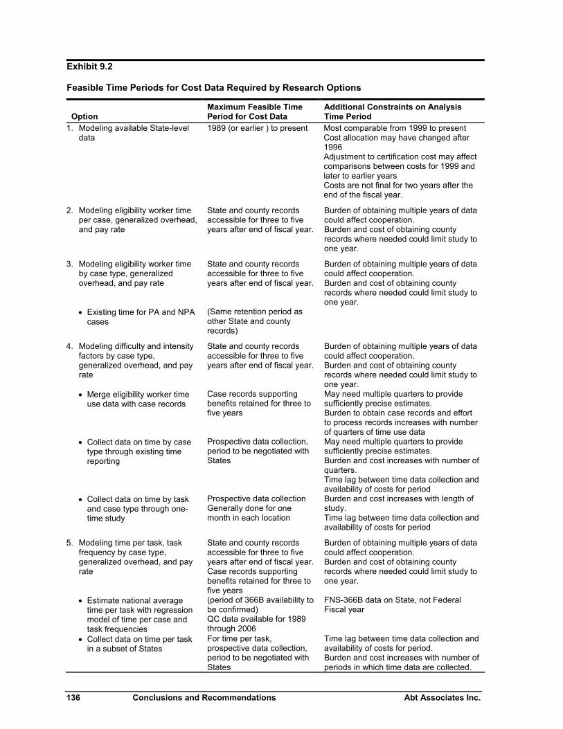
136 Conclusions and Recommendations Abt Associates Inc.
Exhibit 9.2
Feasible Time Periods for Cost Data Required by Research Options
OptionMaximum Feasible TimePeriod for Cost Data
Additional Constraints on AnalysisTime Period
1. Modeling available State-leveldata
1989 (or earlier ) to present Most comparable from 1999 to presentCost allocation may have changed after1996Adjustment to certification cost may affectcomparisons between costs for 1999 andlater to earlier yearsCosts are not final for two years after theend of the fiscal year.
2. Modeling eligibility worker timeper case, generalized overhead,and pay rate
State and county recordsaccessible for three to fiveyears after end of fiscal year.
Burden of obtaining multiple years of datacould affect cooperation.Burden and cost of obtaining countyrecords where needed could limit study toone year.
3. Modeling eligibility worker timeby case type, generalizedoverhead, and pay rate
State and county recordsaccessible for three to fiveyears after end of fiscal year.
Burden of obtaining multiple years of datacould affect cooperation.Burden and cost of obtaining countyrecords where needed could limit study toone year.
Existing time for PA and NPAcases
(Same retention period asother State and countyrecords)
4. Modeling difficulty and intensityfactors by case type,generalized overhead, and payrate
State and county recordsaccessible for three to fiveyears after end of fiscal year.
Burden of obtaining multiple years of datacould affect cooperation.Burden and cost of obtaining countyrecords where needed could limit study toone year.
Merge eligibility worker timeuse data with case records
Case records supportingbenefits retained for three tofive years
May need multiple quarters to providesufficiently precise estimates.Burden to obtain case records and effortto process records increases with numberof quarters of time use data
Collect data on time by casetype through existing timereporting
Prospective data collection,period to be negotiated withStates
May need multiple quarters to providesufficiently precise estimates.Burden and cost increases with number ofquarters.Time lag between time data collection andavailability of costs for period
Collect data on time by taskand case type through one-time study
Prospective data collectionGenerally done for onemonth in each location
Burden and cost increases with length ofstudy.Time lag between time data collection andavailability of costs for period
5. Modeling time per task, taskfrequency by case type,generalized overhead, and payrate
State and county recordsaccessible for three to fiveyears after end of fiscal year.Case records supportingbenefits retained for three tofive years
Burden of obtaining multiple years of datacould affect cooperation.Burden and cost of obtaining countyrecords where needed could limit study toone year.
Estimate national averagetime per task with regressionmodel of time per case andtask frequencies
(period of 366B availability tobe confirmed)QC data available for 1989through 2006
FNS-366B data on State, not FederalFiscal year
Collect data on time per taskin a subset of States
For time per task,prospective data collection,period to be negotiated withStates
Time lag between time data collection andavailability of costs for period.Burden and cost increases with number ofperiods in which time data are collected.
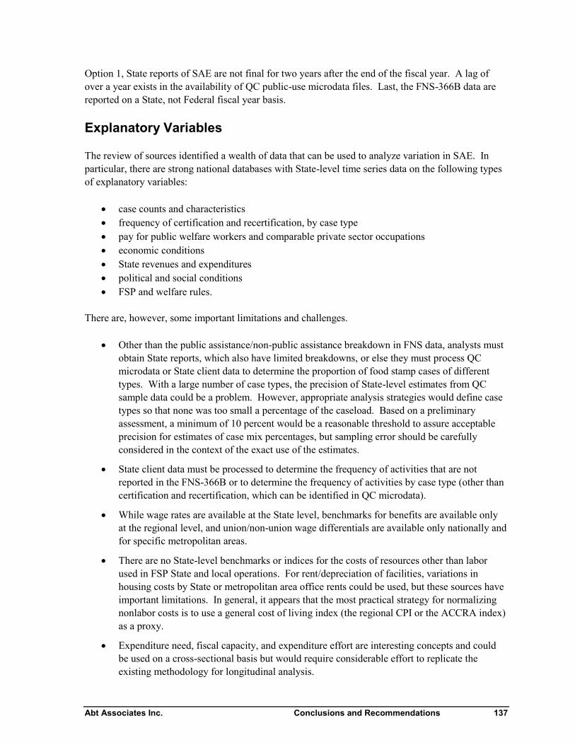
Abt Associates Inc. Conclusions and Recommendations 137
Option 1, State reports of SAE are not final for two years after the end of the fiscal year. A lag ofover a year exists in the availability of QC public-use microdata files. Last, the FNS-366B data arereported on a State, not Federal fiscal year basis.
Explanatory Variables
The review of sources identified a wealth of data that can be used to analyze variation in SAE. Inparticular, there are strong national databases with State-level time series data on the following typesof explanatory variables:
case counts and characteristics frequency of certification and recertification, by case type pay for public welfare workers and comparable private sector occupations economic conditions State revenues and expenditures political and social conditions FSP and welfare rules.
There are, however, some important limitations and challenges.
Other than the public assistance/non-public assistance breakdown in FNS data, analysts mustobtain State reports, which also have limited breakdowns, or else they must process QCmicrodata or State client data to determine the proportion of food stamp cases of differenttypes. With a large number of case types, the precision of State-level estimates from QCsample data could be a problem. However, appropriate analysis strategies would define casetypes so that none was too small a percentage of the caseload. Based on a preliminaryassessment, a minimum of 10 percent would be a reasonable threshold to assure acceptableprecision for estimates of case mix percentages, but sampling error should be carefullyconsidered in the context of the exact use of the estimates.
State client data must be processed to determine the frequency of activities that are notreported in the FNS-366B or to determine the frequency of activities by case type (other thancertification and recertification, which can be identified in QC microdata).
While wage rates are available at the State level, benchmarks for benefits are available onlyat the regional level, and union/non-union wage differentials are available only nationally andfor specific metropolitan areas.
There are no State-level benchmarks or indices for the costs of resources other than laborused in FSP State and local operations. For rent/depreciation of facilities, variations inhousing costs by State or metropolitan area office rents could be used, but these sources haveimportant limitations. In general, it appears that the most practical strategy for normalizingnonlabor costs is to use a general cost of living index (the regional CPI or the ACCRA index)as a proxy.
Expenditure need, fiscal capacity, and expenditure effort are interesting concepts and couldbe used on a cross-sectional basis but would require considerable effort to replicate theexisting methodology for longitudinal analysis.
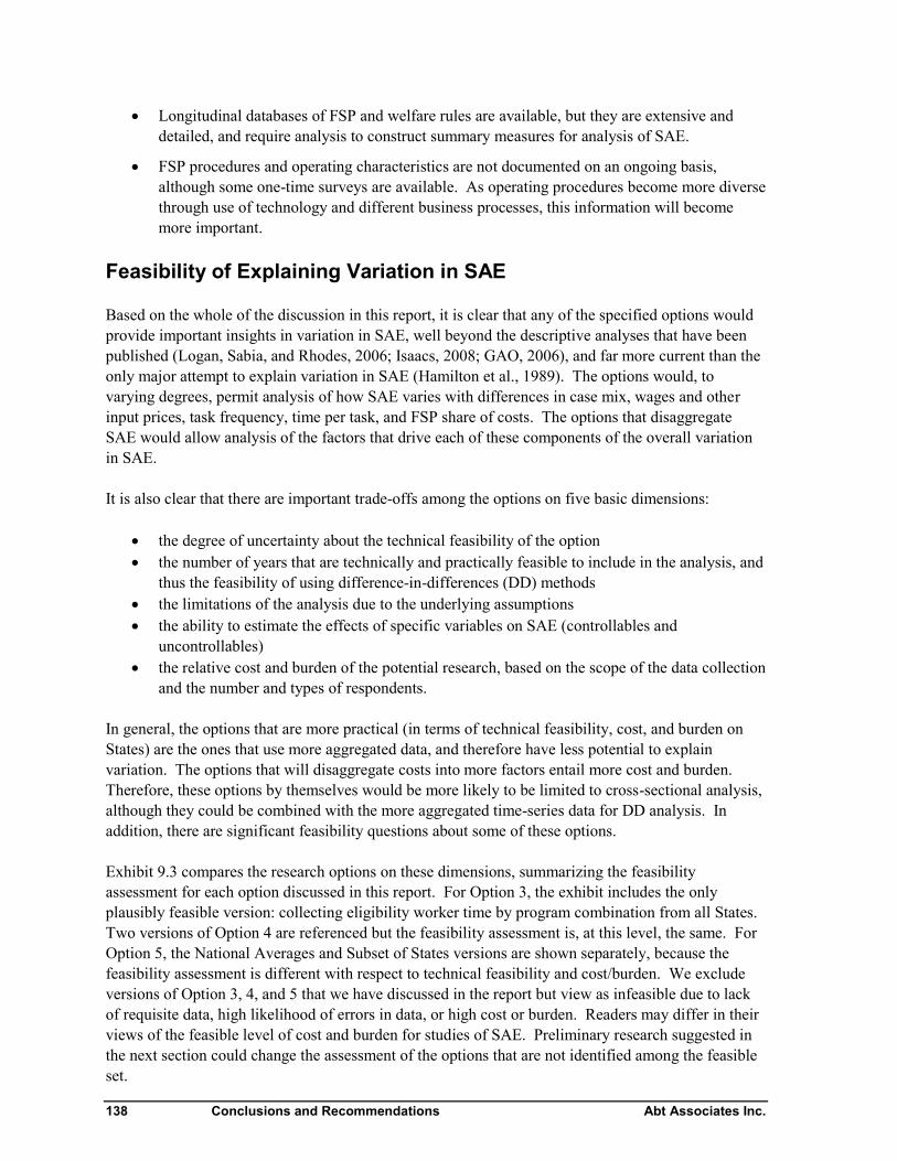
138 Conclusions and Recommendations Abt Associates Inc.
Longitudinal databases of FSP and welfare rules are available, but they are extensive anddetailed, and require analysis to construct summary measures for analysis of SAE.
FSP procedures and operating characteristics are not documented on an ongoing basis,although some one-time surveys are available. As operating procedures become more diversethrough use of technology and different business processes, this information will becomemore important.
Feasibility of Explaining Variation in SAE
Based on the whole of the discussion in this report, it is clear that any of the specified options wouldprovide important insights in variation in SAE, well beyond the descriptive analyses that have beenpublished (Logan, Sabia, and Rhodes, 2006; Isaacs, 2008; GAO, 2006), and far more current than theonly major attempt to explain variation in SAE (Hamilton et al., 1989). The options would, tovarying degrees, permit analysis of how SAE varies with differences in case mix, wages and otherinput prices, task frequency, time per task, and FSP share of costs. The options that disaggregateSAE would allow analysis of the factors that drive each of these components of the overall variationin SAE.
It is also clear that there are important trade-offs among the options on five basic dimensions:
the degree of uncertainty about the technical feasibility of the option the number of years that are technically and practically feasible to include in the analysis, and
thus the feasibility of using difference-in-differences (DD) methods the limitations of the analysis due to the underlying assumptions the ability to estimate the effects of specific variables on SAE (controllables and
uncontrollables) the relative cost and burden of the potential research, based on the scope of the data collection
and the number and types of respondents.
In general, the options that are more practical (in terms of technical feasibility, cost, and burden onStates) are the ones that use more aggregated data, and therefore have less potential to explainvariation. The options that will disaggregate costs into more factors entail more cost and burden.Therefore, these options by themselves would be more likely to be limited to cross-sectional analysis,although they could be combined with the more aggregated time-series data for DD analysis. Inaddition, there are significant feasibility questions about some of these options.
Exhibit 9.3 compares the research options on these dimensions, summarizing the feasibilityassessment for each option discussed in this report. For Option 3, the exhibit includes the onlyplausibly feasible version: collecting eligibility worker time by program combination from all States.Two versions of Option 4 are referenced but the feasibility assessment is, at this level, the same. ForOption 5, the National Averages and Subset of States versions are shown separately, because thefeasibility assessment is different with respect to technical feasibility and cost/burden. We excludeversions of Option 3, 4, and 5 that we have discussed in the report but view as infeasible due to lackof requisite data, high likelihood of errors in data, or high cost or burden. Readers may differ in theirviews of the feasible level of cost and burden for studies of SAE. Preliminary research suggested inthe next section could change the assessment of the options that are not identified among the feasibleset.
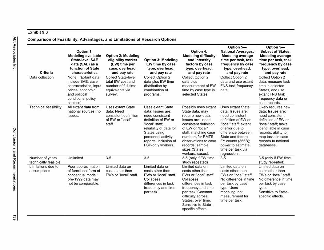
Ab
tA
ssociates
Inc.
Co
nclu
sions
and
Recom
men
datio
ns
139
Exhibit 9.3
Comparison of Feasibility, Advantages, and Limitations of Research Options
Criteria
Option 1:Modeling available
State-level SAEdata (SAE) as a
function of Statecharacteristics
Option 2: Modelingeligibility worker
(EW) time percase, overhead,
and pay rate
Option 3: ModelingEW time by casetype, overhead,
and pay rate
Option 4:Modeling difficulty
and intensityfactors by casetype, overhead,
and pay rate
Option 5—National Averages:Modeling averagetime per task, taskfrequency by case
type, overhead,and pay rate
Option 5—Subset of States:Modeling averagetime per task, taskfrequency by case
type, overhead,and pay rate
Data collection None. (Extant datainclude SAE, casecharacteristics, inputprices, economicand politicalconditions, policychoices).
Collect State-leveltotal EW cost andnumber of full-timeequivalents viasurvey.
Collect Option 2data plus EW timedistribution bycombination ofprograms.
Collect Option 2data plusmeasurement of EWtime by case type inselected States.
Collect Option 2data and use extantFNS task frequencydata.
Collect Option 2data, measure tasktime in selectedStates, and useextant FNS taskfrequency data orcase records.
Technical feasibility All extant data fromnational sources, noissues.
Uses extant Statedata; Needconsistent definitionof EW or "local"staff.
Uses extant Statedata; Issues are:need consistentdefinition of EW or"local" staff;reliability of data forStates usingpersonnel activityreports; inclusion ofFSP-only workers.
Possibly uses extantState data, mayrequire new data.Issues are: needconsistent definitionof EW or "local"staff; matching casenumbers for RMTSobservations to caserecords; samplesizes (States,workers, cases).
Uses extant Statedata; Issues are:need consistentdefinition of EW or"local" staff; extentof error due todifference betweenState and federalFY counts (366B);power to estimatetime per task viaregression .
Likely requires newdata; Issues are:need consistentdefinition of EW or"local" staff; tasksidentifiable in caserecords; ability tomap tasks in caserecords to nationaldatabases.
Number of yearstechnically feasible
Unlimited 3-5 3-5 3-5 (only if EW timestudy repeated)
3-5 3-5 (only if EW timestudy repeated)
Limitations due toassumptions
Poor approximationof functional form ofconceptual model;pre-1999 data maynot be comparable.
Limited data oncosts other thanEWs or “local” staff.
Limited data oncosts other thanEWs or “local” staff.Collapsesdifferences in taskfrequency and timeper task.
Limited data oncosts other thanEWs or “local” staff.Collapsesdifferences in taskfrequency and timeper task. Constantdifficulty acrossStates, over time.Sensitive to State-specific effects.
Limited data oncosts other thanEWs or “local” staff.No difference in timeper task by casetype. Usesmodeling, notmeasurement fortime per task.
Limited data oncosts other thanEWs or “local” staff.No difference in timeper task by casetype.Sensitive to State-specific effects.
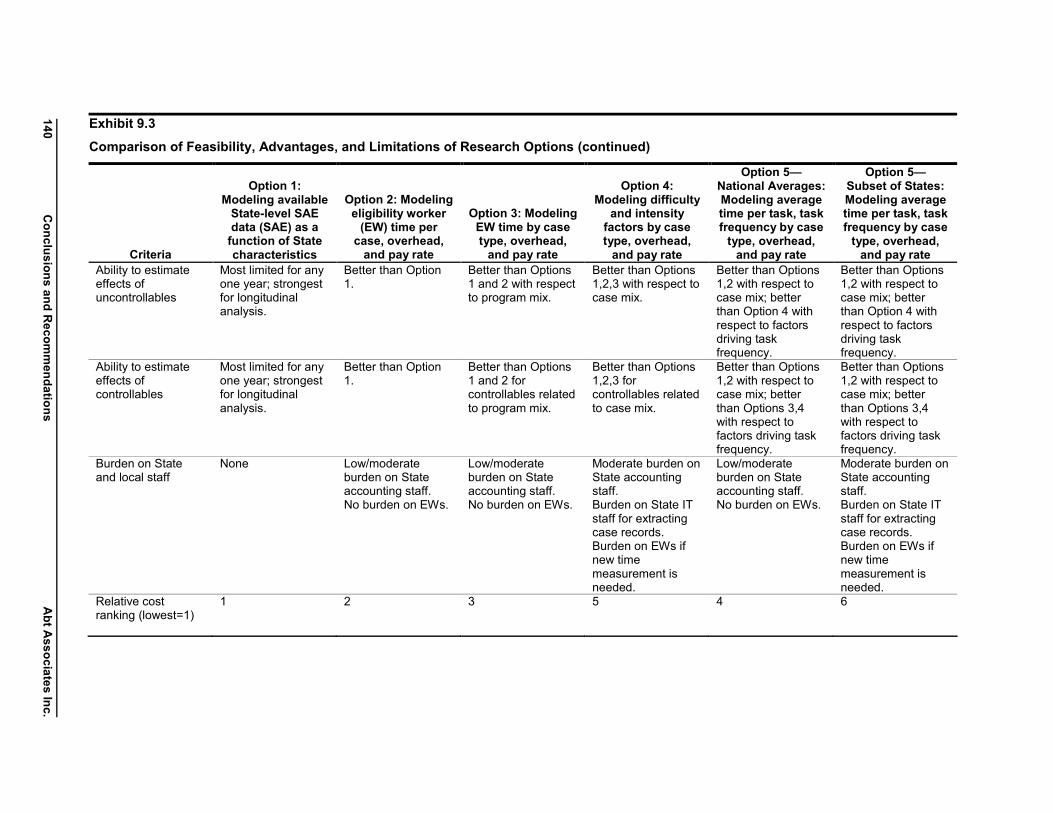
140C
on
clusion
san
dR
ecomm
end
ation
sA
bt
Asso
ciatesIn
c.
Exhibit 9.3
Comparison of Feasibility, Advantages, and Limitations of Research Options (continued)
Criteria
Option 1:Modeling available
State-level SAEdata (SAE) as a
function of Statecharacteristics
Option 2: Modelingeligibility worker
(EW) time percase, overhead,
and pay rate
Option 3: ModelingEW time by casetype, overhead,
and pay rate
Option 4:Modeling difficulty
and intensityfactors by casetype, overhead,
and pay rate
Option 5—National Averages:Modeling averagetime per task, taskfrequency by case
type, overhead,and pay rate
Option 5—Subset of States:Modeling averagetime per task, taskfrequency by case
type, overhead,and pay rate
Ability to estimateeffects ofuncontrollables
Most limited for anyone year; strongestfor longitudinalanalysis.
Better than Option1.
Better than Options1 and 2 with respectto program mix.
Better than Options1,2,3 with respect tocase mix.
Better than Options1,2 with respect tocase mix; betterthan Option 4 withrespect to factorsdriving taskfrequency.
Better than Options1,2 with respect tocase mix; betterthan Option 4 withrespect to factorsdriving taskfrequency.
Ability to estimateeffects ofcontrollables
Most limited for anyone year; strongestfor longitudinalanalysis.
Better than Option1.
Better than Options1 and 2 forcontrollables relatedto program mix.
Better than Options1,2,3 forcontrollables relatedto case mix.
Better than Options1,2 with respect tocase mix; betterthan Options 3,4with respect tofactors driving taskfrequency.
Better than Options1,2 with respect tocase mix; betterthan Options 3,4with respect tofactors driving taskfrequency.
Burden on Stateand local staff
None Low/moderateburden on Stateaccounting staff.No burden on EWs.
Low/moderateburden on Stateaccounting staff.No burden on EWs.
Moderate burden onState accountingstaff.Burden on State ITstaff for extractingcase records.Burden on EWs ifnew timemeasurement isneeded.
Low/moderateburden on Stateaccounting staff.No burden on EWs.
Moderate burden onState accountingstaff.Burden on State ITstaff for extractingcase records.Burden on EWs ifnew timemeasurement isneeded.
Relative costranking (lowest=1)
1 2 3 5 4 6
Abt Associates Inc. Conclusions and Recommendations 141
Option 1, the modeling of existing aggregate State-level SAE data, is by far the most feasible option.There is no doubt about the technical feasibility, and it has the lowest cost and burden of the options.It is also the only option that by itself would support a robust DD analysis. It could readily becombined with any of the other options as an initial exploratory stage or as a complement. On theother hand, Option 1 uses the most aggregated cost data. This is a very important limiting factor onthe ability to model the effects of specific variables of interest, particularly in the domains of FSPpolicies and management choices. Other limitations are the assumed functional form and theuncertain comparability between pre-1999 data and later years. For explanatory variables that changesubstantially within States over time, the ability to conduct longitudinal analysis using DD or otherappropriate methods somewhat mitigates the limitation of aggregate data. We note that the linearspecification under Option 1 is a poor approximation of the true functional form indicated by ourconceptual framework. The other options more nearly approximate the functional form.
Option 2, Option 3, and Option 5-National Averages would use existing data from State accountingreports or spreadsheets and are therefore also likely to be feasible. (The feasible version of Option 3would collect existing data on eligibility worker time distribution by program combination.) Becauseof the use of existing aggregate accounting data in State records, these options rank second, third, andfourth (respectively) in expected cost. These options would have low to moderate burden on Stateaccounting personnel and no burden on eligibility workers. The cost and burden would depend inpart on the extent of data collected on eligibility worker pay and characteristics, and on thecomposition of overhead. These options would substantially improve the ability to identify majorfactors associated with variation in SAE. All three options would allow separate analysis of variationin eligibility worker time, pay, and overhead. Option 3 would add further insight into the effects ofcost-sharing among programs, while Option 5-National Averages would add insights into the factorsdriving task frequency and their impacts on SAE. Key limitations for these three options, as well asthe more costly options, would be: the challenge of consistently measuring eligibility worker timeand costs, limited data on overhead, and the simplification of all costs other than eligibility workerpay as overhead. In addition, there would be a challenge to collect accounting data and case recordsin States—including California, New York, and eight others—where counties administer the FSP.These issues appear to be surmountable, but they would add to the cost and burden of a study.
In practice, it would be natural to combine Option 2 with Option 3, Option 5-National Averages, orboth. On top of the data for Option 2, the additional data from States for the feasible version ofOption 3 would be quite modest, and Option 5-National Averages would not require any additionalState data. The potential insights from these two options would be complementary, and each wouldoffset the other’s limitations.
A limited version of Option 5-All States based on interviews with State experts is not listed in theexhibit but could be implemented at a low cost and no burden to eligibility workers. If feasible, thisversion would provide the ability to compare States in terms of their own eligibility worker time pertask, rather than relying on averages estimated from national data (the National Averages version) orfrom selected States (the Subset of States version). There is real uncertainty about the level ofaccuracy for interview-based estimates and the validity of the methodology in this context, whenState responses will be explicitly compared in the study results. Therefore, we view this option as apotential adjunct to other options, rather than a primary option on its own.
Option 4 and Option 5-Subset of States would provide the richest data (among the options that weconsider feasible) and, on balance, the best opportunities to identify the factors associated with
142 Conclusions and Recommendations Abt Associates Inc.
variation in SAE. Both options would generalize from data collected in a sample of States. Asindicated in Exhibit 9.3, Option 4 would collect eligibility worker time by case type in selected Statesto estimate standard difficulty factors for case types. Option 5-Subset of States would collecteligibility worker time per task in selected States to estimate the average time per task. These optionsare clearly strongest for estimating the variation associated with factors that do not changesubstantially within States over the time period that is feasible to study. It is unclear whether factorsthat are susceptible to longitudinal analysis would be better assessed with Option 1, but on balance itappears likely that the Options 4 and 5 would have more explanatory power. The disaggregation ofSAE would allow more focused analysis of the variables that are relevant to each of the sixcomponents of variation (FSP share, case mix, overhead, eligibility worker pay, task frequency, andtime per task; Option 4 collapses the last two components). This analysis does depend on thesimplifying assumptions of these options, but the alternative would be much more costly andburdensome studies.
The practical downside of these options is that they require more data and thus would be more costlythan the other four options.85 Option 4 may be feasible to implement without collecting new datafrom eligibility workers, provided that existing RMTS data can be merged with case records. It ispossible that some States have existing data for one of these options, but this seems unlikely. Option5-Subset of States in particular seems likely to require data collection from eligibility workers, or atleast from their supervisors, but survey or interview methods could be used to reduce the burden.
While Option 4 and Option 5-Subset of States would complement each other, there may be a need tochoose between them. This choice is not clear, because of several unknown feasibility questions: theavailability of existing data that would facilitate these options, the feasibility of matching RMTS datawith case records, the tasks identifiable in case records, and the sample size requirements for specificdata collection approaches. In addition, analysis conducted via Option 1 might shed light on therelative importance of case mix and task frequency, and on the relationship between these factors.This analysis might point to one of these options as the more likely to explain variation in SAE.
Beyond these specific trade-offs among the options, there are some important limitations for potentialstudies of the variation in SAE. First, both the structure of State accounting systems and the availableprice index data pose challenges for analyzing the impacts of input prices other than pay and benefits.Second, special-purpose surveys may be needed to identify which States use management practicesthat are hypothesized to affect SAE: these include variations on the conventional staffing and clientflow of local food stamp offices and newer, more radical changes. FNS has undertaken such asurvey, but a time series of such data is desirable for future analyses. Finally, while countyadministration of the FSP may pose some challenges for collecting data on SAE, it also offers someopportunities. Where comprehensive FSP costs are determined for individual counties, there is thepotential for comparisons within States to examine the impacts of scale and of policies and practicesthat vary within States, while controlling for conditions that vary between States but are consistentwithin the State.
The feasibility of all of these options depends on the cooperation of State agencies and, at least insome States, county agencies as well. Options 2 through 5 would require the cooperation of
85 While the options are numbered 1 through 5, there are two different versions of Option 5 among thoselisted in Exhibit 9.3.
Abt Associates Inc. Conclusions and Recommendations 143
accounting personnel. New data collection from eligibility workers would require consent fromagency managers and may require consent from individual workers or their collective representatives.
We have sought to identify options that make the most use of existing data, and options that can beintegrated into agency operations, in order to minimize the burden on operational workers and theinterference with operations. We have also taken into account the potential burden on accountingpersonnel. The design of future studies would need to address the perceived risks and benefits of thestudies to State and local personnel. Depending on the extent of the desired data collection, it may beappropriate to consider incentives or mandates for participation, or ways to integrate data collectionwith FNS oversight so as to leverage FNS’ influence. Another potential strategy for gainingcooperation is to engage key opinion leaders among the State food stamp directors in planning thestudy and interpreting the results. This would tap their knowledge while making it clear that thestudy is intended to help them manage the FSP.
Finally, we note the critical importance of taking State performance into account when makingcomparisons of SAE and interpreting differences in SAE among the States. A State with a low levelof SAE per case, even after adjusting for uncontrollables such as case mix and labor markets, is onlymore efficient than States with higher levels of SAE per case if its performance is as good or better.We have suggested ways to use each of the options to estimate a normalized cost per case as a basisfor comparisons of performance on the key dimensions of accuracy, timeliness, and access.
A Suggested Program of Research on Variation in SAE
Based on the preceding data assessment, we suggest a sequence of concepts for feasible andinformative studies of variation in SAE. While we present them as discrete studies, we show howeach study would help guide others presented later in the sequence. In developing this sequence, wewere mindful of the lack of knowledge about what are actually the important sources of variation inSAE and the potential cost of the studies that would provide richer data. Thus, the sequence beginswith Studies 1 and 2, which are the least expensive approaches and include strategies that wouldresolve uncertainties about the feasibility and potential value of more expensive approaches. Studies3, 4, and 5 are suggested as intermediate steps between the most basic studies (Studies 1 and 2) andthe most ambitious studies (Studies 6, 7, and 8). These last three studies are presented as alternativesfor implementing the approaches that would provide the richest data—Option 4 or Option 5-Subset ofStates. Exhibit 9.4 summarizes the studies, their prerequisites, their key data, their expectedcontributions to understanding of interstate variation in SAE, and their relative expected cost. In thisexhibit, “low” cost means expected cost under $500,000; “moderate” cost means expected costbetween $500,000 and $1,000,000; and “high” cost means expected cost more than $1,000,000. Theexpectations are based on confidential estimates provided separately to FNS. The combined cost ofmultiple studies conducted together would be somewhat less than the sum of the cost of the studiesconducted separately, because of the integration of study design and reporting.
Study 1: Exploratory Analysis of Existing Aggregate Cost Data
This study would analyze existing aggregate cost data, as in Option 1, using reduced form difference-of-difference regressions. We view this as a relatively modest, low-cost first step that could provideimmediate insights and identify directions for future research. The primary focus would be on time-series regression analysis of certification costs (potentially using both narrow and broad definitions),but the scope could be expanded to include the costs of other functions could be analyzed as well.
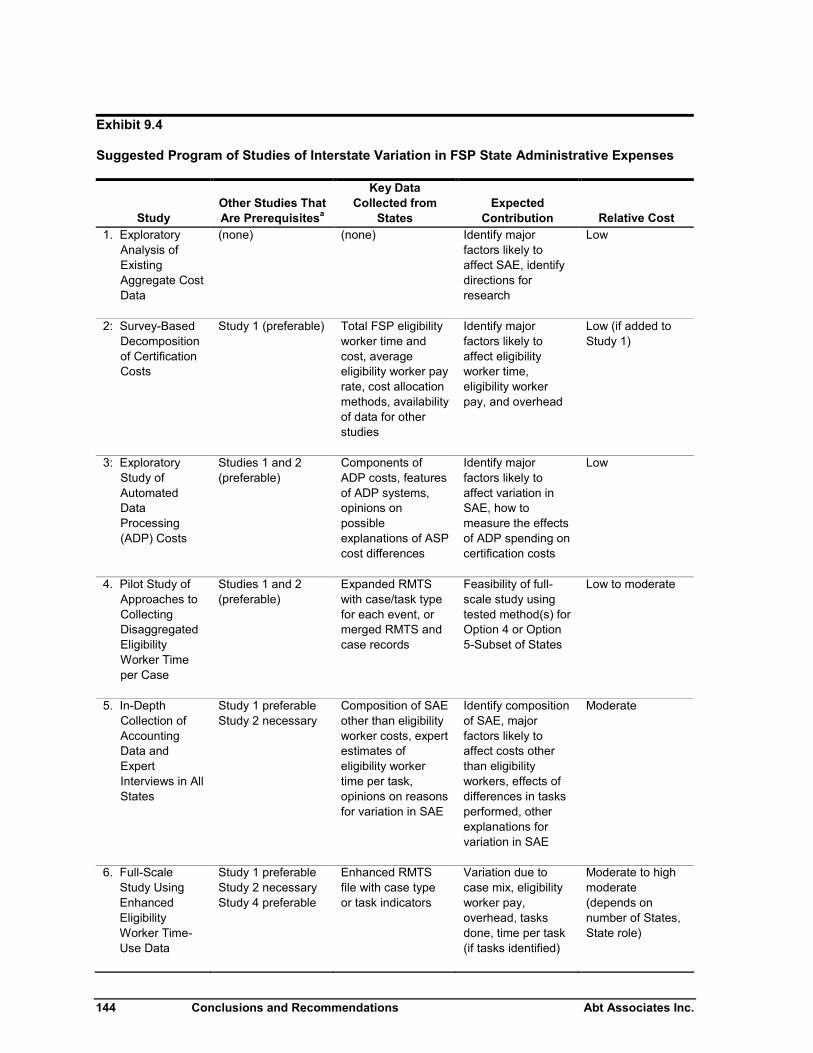
144 Conclusions and Recommendations Abt Associates Inc.
Exhibit 9.4
Suggested Program of Studies of Interstate Variation in FSP State Administrative Expenses
StudyOther Studies ThatAre Prerequisitesa
Key DataCollected from
StatesExpected
Contribution Relative Cost1. Exploratory
Analysis ofExistingAggregate CostData
(none) (none) Identify majorfactors likely toaffect SAE, identifydirections forresearch
Low
2: Survey-BasedDecompositionof CertificationCosts
Study 1 (preferable) Total FSP eligibilityworker time andcost, averageeligibility worker payrate, cost allocationmethods, availabilityof data for otherstudies
Identify majorfactors likely toaffect eligibilityworker time,eligibility workerpay, and overhead
Low (if added toStudy 1)
3: ExploratoryStudy ofAutomatedDataProcessing(ADP) Costs
Studies 1 and 2(preferable)
Components ofADP costs, featuresof ADP systems,opinions onpossibleexplanations of ASPcost differences
Identify majorfactors likely toaffect variation inSAE, how tomeasure the effectsof ADP spending oncertification costs
Low
4. Pilot Study ofApproaches toCollectingDisaggregatedEligibilityWorker Timeper Case
Studies 1 and 2(preferable)
Expanded RMTSwith case/task typefor each event, ormerged RMTS andcase records
Feasibility of full-scale study usingtested method(s) forOption 4 or Option5-Subset of States
Low to moderate
5. In-DepthCollection ofAccountingData andExpertInterviews in AllStates
Study 1 preferableStudy 2 necessary
Composition of SAEother than eligibilityworker costs, expertestimates ofeligibility workertime per task,opinions on reasonsfor variation in SAE
Identify compositionof SAE, majorfactors likely toaffect costs otherthan eligibilityworkers, effects ofdifferences in tasksperformed, otherexplanations forvariation in SAE
Moderate
6. Full-ScaleStudy UsingEnhancedEligibilityWorker Time-Use Data
Study 1 preferableStudy 2 necessaryStudy 4 preferable
Enhanced RMTSfile with case typeor task indicators
Variation due tocase mix, eligibilityworker pay,overhead, tasksdone, time per task(if tasks identified)
Moderate to highmoderate(depends onnumber of States,State role)
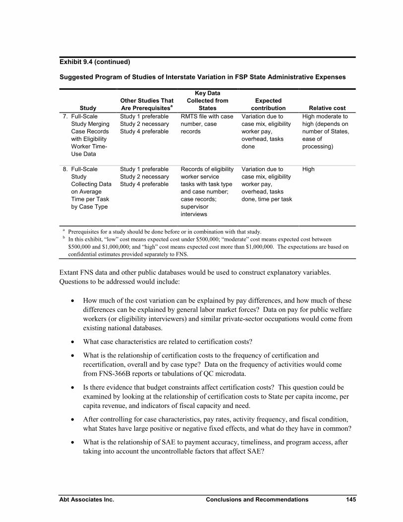
Abt Associates Inc. Conclusions and Recommendations 145
Exhibit 9.4 (continued)
Suggested Program of Studies of Interstate Variation in FSP State Administrative Expenses
StudyOther Studies ThatAre Prerequisitesa
Key DataCollected from
StatesExpected
contribution Relative cost7. Full-Scale
Study MergingCase Recordswith EligibilityWorker Time-Use Data
Study 1 preferableStudy 2 necessaryStudy 4 preferable
RMTS file with casenumber, caserecords
Variation due tocase mix, eligibilityworker pay,overhead, tasksdone
High moderate tohigh (depends onnumber of States,ease ofprocessing)
8. Full-ScaleStudyCollecting Dataon AverageTime per Taskby Case Type
Study 1 preferableStudy 2 necessaryStudy 4 preferable
Records of eligibilityworker servicetasks with task typeand case number;case records;supervisorinterviews
Variation due tocase mix, eligibilityworker pay,overhead, tasksdone, time per task
High
a Prerequisites for a study should be done before or in combination with that study.b In this exhibit, “low” cost means expected cost under $500,000; “moderate” cost means expected cost between
$500,000 and $1,000,000; and “high” cost means expected cost more than $1,000,000. The expectations are based onconfidential estimates provided separately to FNS.
Extant FNS data and other public databases would be used to construct explanatory variables.Questions to be addressed would include:
How much of the cost variation can be explained by pay differences, and how much of thesedifferences can be explained by general labor market forces? Data on pay for public welfareworkers (or eligibility interviewers) and similar private-sector occupations would come fromexisting national databases.
What case characteristics are related to certification costs?
What is the relationship of certification costs to the frequency of certification andrecertification, overall and by case type? Data on the frequency of activities would comefrom FNS-366B reports or tabulations of QC microdata.
Is there evidence that budget constraints affect certification costs? This question could beexamined by looking at the relationship of certification costs to State per capita income, percapita revenue, and indicators of fiscal capacity and need.
After controlling for case characteristics, pay rates, activity frequency, and fiscal condition,what States have large positive or negative fixed effects, and what do they have in common?
What is the relationship of SAE to payment accuracy, timeliness, and program access, aftertaking into account the uncontrollable factors that affect SAE?
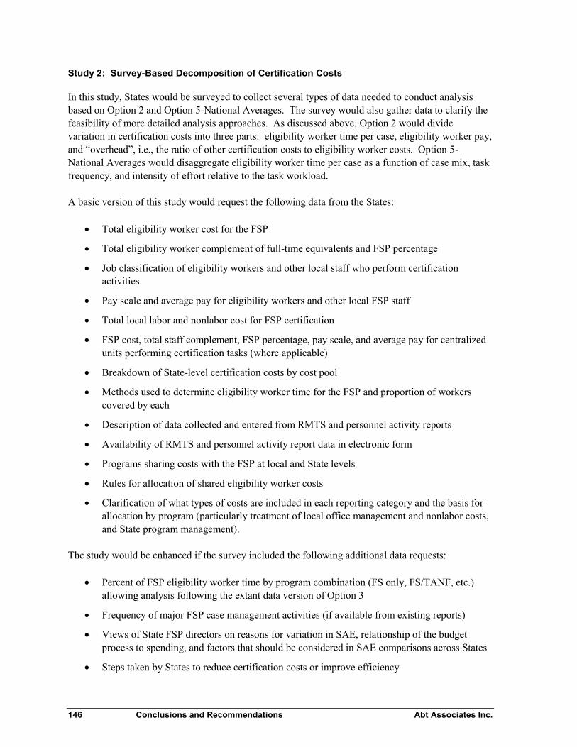
146 Conclusions and Recommendations Abt Associates Inc.
Study 2: Survey-Based Decomposition of Certification Costs
In this study, States would be surveyed to collect several types of data needed to conduct analysisbased on Option 2 and Option 5-National Averages. The survey would also gather data to clarify thefeasibility of more detailed analysis approaches. As discussed above, Option 2 would dividevariation in certification costs into three parts: eligibility worker time per case, eligibility worker pay,and “overhead”, i.e., the ratio of other certification costs to eligibility worker costs. Option 5-National Averages would disaggregate eligibility worker time per case as a function of case mix, taskfrequency, and intensity of effort relative to the task workload.
A basic version of this study would request the following data from the States:
Total eligibility worker cost for the FSP
Total eligibility worker complement of full-time equivalents and FSP percentage
Job classification of eligibility workers and other local staff who perform certificationactivities
Pay scale and average pay for eligibility workers and other local FSP staff
Total local labor and nonlabor cost for FSP certification
FSP cost, total staff complement, FSP percentage, pay scale, and average pay for centralizedunits performing certification tasks (where applicable)
Breakdown of State-level certification costs by cost pool
Methods used to determine eligibility worker time for the FSP and proportion of workerscovered by each
Description of data collected and entered from RMTS and personnel activity reports
Availability of RMTS and personnel activity report data in electronic form
Programs sharing costs with the FSP at local and State levels
Rules for allocation of shared eligibility worker costs
Clarification of what types of costs are included in each reporting category and the basis forallocation by program (particularly treatment of local office management and nonlabor costs,and State program management).
The study would be enhanced if the survey included the following additional data requests:
Percent of FSP eligibility worker time by program combination (FS only, FS/TANF, etc.)allowing analysis following the extant data version of Option 3
Frequency of major FSP case management activities (if available from existing reports)
Views of State FSP directors on reasons for variation in SAE, relationship of the budgetprocess to spending, and factors that should be considered in SAE comparisons across States
Steps taken by States to reduce certification costs or improve efficiency
Abt Associates Inc. Conclusions and Recommendations 147
Qualifications for eligibility worker and other job classifications performing certificationtasks.
Average years of experience of eligibility workers.
Structure of local office operations (specialization of workers and units by program orfunction).
Automated data processing system features expected to affect costs or worker productivity.
The study would combine these data with existing data on SAE caseload characteristics, policyoptions, factor prices, and political, economic, and social conditions. The analysis would model thethree elements of Option 2: eligibility worker time per case, eligibility worker pay, and overhead.Additional analysis would implement Option 5-National Averages with the eligibility worker timedata and data on task frequency by case type from FNS sources. If data on eligibility worker time byprogram combination were collected, the analysis specified under Option 3 would be implemented.
The cost of this study would be low if it were added to Study 1, and the exploratory analysis ofaggregate data would help guide the analysis of the more disaggregated data and the data sought inthe survey. A State survey could also be combined with any of the other concepts described below.
Study 3: Exploratory Study of Automated Data Processing Costs
As suggested in this report, there is considerable interest in the role of automated data processingcosts, both as a component of SAE and as a possible investment with payoffs in productivity of FSPoperations. While simple analysis of variation in ADP costs could be done as part of the ExploratoryAnalysis study, a three-part approach would be more insightful:
Descriptive analysis of differences and trends in ADP development and operations costs, andtheir relationship to characteristics of States and their FSP operations
Investigation and analysis of available comparative information on the capabilities and keydesign features of ADP systems used for the FSP, cross-referenced to the cost data
Collection and analysis of further data, through interviews and review of documents, toexamine the differences between high-cost and low-cost States not readily explained by theextant data.
Under the ideal sequence, Study 1 and Study 2 would be conducted before Study 3. One could thenexamine the characteristics and costs of ADP systems in States with high (or low) performancerelative to their normalized SAE per case (adjusted for case mix, market wages, economic conditions,and other uncontrollables). The cost of Study 3 would be low.
Study 4: Pilot Study of Approaches to Collecting Disaggregated Eligibility Worker Time perCase
Given the variety of methods that might be used to disaggregate eligibility worker time per case bycase type or activity, it may be worthwhile to test these methods on a limited scale before undertakinga full-scale study. In particular, there are two methods of gathering detailed eligibility worker timedata for Options 4 and 5 that appear potentially feasible but have not been used before: (a) mergingRMTS data with case data, and (b) expanding an existing RMTS to include task information. These
148 Conclusions and Recommendations Abt Associates Inc.
methods would be particularly worthy of pilot-testing in one or more States. The goal of this pilotstudy would be to gain a better understanding of the potential, limitations, and cost of the methods.Thus, samples collected would be smaller than the size needed to meet the standards of precision for afull-scale study; data would be collected from States that volunteer or otherwise would provide easiersettings for the test, rather than from a more representative group of States. The other suggestedmethods of collecting data from eligibility workers (event logs and surveys) have been used for FSPstudies, so there is less intrinsic need to test them (beyond the standard pretest for clearance of datacollection). On the other hand, including these methods would allow tests of multiple approaches inthe same States; comparisons of results would provide insights about the relative feasibility andvalidity of the approaches. In addition, there would be synergies in using the same case record filesfor more than one approach.
The cost of Study 4 would be low to moderate, depending on the number of approaches tested, thenumber of States, and the role of the States. Some States might be willing to take on some of the costof the test in order to have access to the results (e.g., training workers to complete new forms,processing the merge of RMTS and case records, etc.), while others might expect the researchers tocarry out all of the data collection and processing.
Study 5: In-Depth Collection of Accounting Data and Expert Interviews in All States
Although data for Option 2 and Option 5-National Averages would be collected by survey, Study 2would probably identify some significant unknowns that would warrant more in-depth data collection.Therefore, a natural follow-up study would collect three kinds of data in each State: accounting datafor the decomposition of overhead, expert estimates of the eligibility worker time per task, anddiscussion of the reasons for variation in SAE. The accounting data would be collected to attempt thedecomposition of overhead by level (local/State), between labor and nonlabor, and breaking out keynonlabor costs such as rent. The estimates of eligibility worker time per task would be obtainedthrough interviews with key informants, such as trainers, business analysts, or managers withextensive knowledge of local operations. These data would permit implementation of the feasibleversion of Option 5-All States. During the course of the contacts for these two data collections, therewould be an excellent opportunity to discuss the findings of studies of SAE, both in general and withrespect to each State individually. These discussions would help get “inside the black box” tounderstand the findings and suggest future directions for research. The cost of such a study, includingdesign, data collection, analysis, and reporting, would be moderate; a low-cost version could be doneif the data collection were limited to 15 or fewer States.
Study 6: Full-Scale Study Using Enhanced Eligibility Worker Time-Use Data
This study has the potential to be the least costly of the three approaches that appear to be feasibleways to implement Option 4 or Option 5-Subset of States. In a representative group of States, theRMTS or personnel activity report would be modified to capture data on the type of case served, thetask, or both for each recorded event. Recording the task is the modification most likely to befeasible, because eligibility workers will always know this, but they may not have immediate accessto the information needed to determine the case type. There are two different scenarios, withdifferent cost implications.
Under one scenario, the researchers collaborate with the State to modify the forms, and the Statecarries out the data collection and tabulates the data. The data collection includes training for workers
Abt Associates Inc. Conclusions and Recommendations 149
and supervisors, sampling workers (and moments for RMTS), distributing and collecting forms, andtracking and following up on missing forms. In a paper system, processing includes data entry andcleaning; an automated system eliminates the former but not the latter. Thus, the cost for theresearchers would be limited to the up-front costs of design and the back-end costs of constructinganalytic files, analysis, and reporting. The cost of such a study in five to seven States would bemoderate.
Under the other scenario, the researchers would implement the study. The State would approve theforms and supply the sample frame, and the researchers would do the rest. The most efficientsolution would be an automated, web-based survey, but there are likely to be major hurdles in settingthis up from outside the State Agency. Instead, the second-best alternative would be a telephone-based system, akin to a random-digit-dial survey. For this scenario, the cost in five to seven Stateswould be moderate to high moderate. (“High moderate” means at the high end of the moderaterange.) These costs do not include the additional burden on the workers, but this would be quitesmall for each worker if the RMTS were implemented statewide over several months.
Study 7: Full-Scale Study Merging Case Records with Eligibility Worker Time-Use Data
This approach also appears to be a feasible way to implement Option 4 or Option 5-Subset of States,and it would be less burdensome to individual workers than the alternatives for these options (Study 6and Study 8). In a representative group of States, researchers would collect and merge two data sets:RMTS or activity report data in electronic form with a case number for each event, and case recordsfor the same time period. As discussed above, a pilot test of this method is recommended beforeundertaking a full-scale study, to resolve technical uncertainties and better understand the cost to theState and to FNS. Efforts for the study would include: designing the sample and analysis, securingState cooperation and access to data, obtaining and processing files, and analysis and reporting.Because of the use of case records in addition to RMTS data, this study would be more costly thanStudy 6: the cost would be high moderate to high, depending on the number of States and the ease ofprocessing their data.
Study 8: Full-Scale Study Collecting Data on Average Time per Task by Case Type
This study would essentially replicate the 1989 certification cost study, which was conducted in fourStates. Eligibility workers in selected offices would record each task for a specified period (such as amonth), including the type of task, the duration, and the case type or case number. Supplementarytime per task data might be collected from supervisors and support staff via interviews or surveys.Tests for differences in average time per task by case type would be conducted. Case records wouldbe analyzed to determine the frequency of the tasks and the relationship of case characteristics to taskfrequency. Data from the States with the in-depth data collection would be combined with aggregatedata for all States (SAE, case characteristics, economic conditions, etc.) for an analysis combining theapproaches of Options 4 and 5. The cost of Study 8 would be high. As noted earlier, the 1989 studycost was $2.3 million in current dollars; this provides a very rough guide for the potential cost of sucha study.

150 Conclusions and Recommendations Abt Associates Inc.
Abt Associates Inc. Background on Food Stamp Program Administration A-1
Appendix A
Background on Food Stamp ProgramAdministration
This appendix presents background information for this report on the administration of the FSP. Itbegins with an overview of the administrative functions of State and local agencies. The appendixthen describes the typical administrative structure of States and local agencies and its variants. (FNShas its own administrative functions, but these are not relevant to studies of State administrativeexpenses.)
FSP Administrative Functions
The primary administrative functions of State and local agencies in the FSP are certification ofeligible households and issuance of benefits. In addition, these agencies provide two kinds ofservices to eligible households: employment and training (E&T) services for adults who are subjectto work requirements, and nutrition education for income-eligible adults and children. Some keysupport functions are automated data processing (ADP), Quality Control (QC), fraud control, andfair hearings. State and local agencies also carry out other administrative functions in support ofcertification, issuance, and provision of FSP services.
The description below of FSP administrative functions reflects operations from approximately 1990to the present, with primary emphasis on how the FSP has operated in the last 10 years. We assumethat data prior to 1990 are not likely to be used in analyses of variation in SAE. The reasons for thisassumption are discussed in the report.
Certification
Certification activities include the processing of initial applications for Food Stamp benefits, periodicrecertification of Food Stamp households, and other actions to obtain, verify, and apply informationon households’ FSP eligibility and entitlement to benefits. These activities are generally performed inlocal FSP offices by State or local government employees. Some States use centralized call centersfor some activities that do not require face-to-face contact, including certification or recertificationinterviews conducted under waivers. Also, applicants in some States use on-line applications with orwithout assistance from community organizations (GAO, 2007). Local FSP offices usually performcertification tasks for other State-administered non-FSP cash assistance programs (such as TemporaryAssistance for Needy Families or TANF and General Assistance) and often for medical assistance,low income energy assistance, and other means-tested programs for low-income residents.
Issuance of Benefits
Over the history of the FSP, States have mainly used one of two systems to issue FSP benefits.Originally, all States issued benefits in the form of paper “food stamp coupons” to recipients (thus thename of the program). State methods of issuing those stamps varied (including State, local andcontractor operations).
A-2 Background on Food Stamp Program Administration Abt Associates Inc.
More recently, States have switched over to issuing FSP benefits through an electronic benefittransfer (EBT) system, which is similar to a debit card system.86 In 1993, Maryland became the firstState to replace the coupon issuance system with EBT. By FY 2005, all FSP households receivedbenefits via EBT. Nearly all States contract with private firms to operate their EBT systems, butsome issuance-related functions (such as card issuance) may be performed at local FSP offices (FNS,2008b). A very small proportion of FSP benefits (less than 0.2 percent) are issued in cash as asupplement to SSI or State aid to elderly or disabled persons.87 This program option is confined to alimited number of States or project areas.
Employment and Training
Each State provides FSP employment and training (E&T) services for FSP recipients who are subjectto job search and work requirements. E&T services are provided through local FSP/TANF officesand other agencies, such as workforce development agencies and community-based organizations.(GAO, 2003) Allowable E&T components include supervised job search, job search training, workexperience or workfare, vocational training, work-related education, and self-employment training.
Nutrition Education
Since 1992, States have had the option of providing nutrition education to persons who are eligiblefor food stamp benefits, with the goal of promoting healthy food and lifestyle choices. Most Stateshave agreements with the State Cooperative Extension Service, State universities, or other agencies toprovide food stamp nutrition education (FSNE). FSNE grew from 7 States in FY 1992 to all 50States and the District of Columbia by FY2005.
Automated Data Processing System Development and Operations
Each State operates a computer system to support FSP operations, usually as part of an integratedeligibility system that also supports TANF and other means-tested programs such as State GeneralAssistance, Medicaid, or the Low Income Home Energy Assistance Program. Some State FoodStamp Agencies operate their own computer centers, while others contract out this function or use acenter that services multiple State agencies.88 In some States the FSP is county-operated (such asNorth Carolina), the State operates the ADP system, and some counties supplement this system withadditional ADP systems; in others, such as California, individual counties operate their own ADPsystems, but there is also a statewide FSP recipient database. Automated data processing (ADP) costsinclude development of new or upgraded systems, operation and maintenance of computer hardwareand software, data communications networks, and local office equipment.
86 Nearly all States use “on-line” EBT systems, in which a terminal at the point of sale interacts with a central“host” computer to debit the recipient’s account. Wyoming and Ohio implemented “off-line” EBTsystems, in which benefit data are stored in a card equipped with a computer chip, transactions areauthorized by the card, and the point of sale terminal later submits a file of transactions to the “host” forsettlement. Ohio converted to an on-line EBT system in 2006, and Wyoming converted to on-line EBT in2007.
87 These cash-out arrangements exist in a limited group of States and do not include the cash in lieu of foodstamp benefits for SSI recipients in California, who are not considered food stamp recipients.
88 Source: Interview with FNS grants management officials, October 2007.
Abt Associates Inc. Background on Food Stamp Program Administration A-3
Fraud Control and Fair Hearings
State and local FSP agencies investigate evidence of fraud by recipients through review of caserecords, interviews with recipients, and third-party sources of information. Fraud investigations mostoften involve misrepresentation of eligibility or dual participation, but other types of investigationsdeal with false reports of lost benefits and trafficking in benefits. When the FSP agency findsevidence of fraud, it may initiate recovery of funds, termination of benefits, or prosecution. FSPagencies conduct fair hearings upon request by applicants or recipients who are subjected to adverseaction (benefit reduction or termination).
Other State and Local Program Administration
State and local FSP agencies carry out a number of other administrative functions, including qualitycontrol, management evaluation, outreach, demonstration projects, and oversight of programoperations. Under the mandatory quality control (QC) system, each State must review a sample ofactive FSP cases and a sample of closed or denied cases to determine whether the determination ofeligibility and benefits is correct. Each State must also conduct management evaluation reviews oflocal office operations.
Composition of Total SAE
Exhibit A-1 shows the percentage distribution of the national total FSP administrative cost for theperiod from 1989 to 2005 (summed over all 17 years) among FSP administrative activities.Certification was by far the largest category, representing three-fifths (59.1%) of the total. Thispercentage was essentially the same over the 17 years in the study. The average total annual cost forcertification was $2.54 billion. The next largest categories were unspecified other (8.5%), issuance(7.2%), employment and training (E&T) services (7.1%), and automated data processing (ADP)operations (5.9%). (“Unspecified other” is the category for costs not reported elsewhere, and so thescope of these costs may have varied from State to State or over time.) The smallest categories weremiscellaneous, fraud control, food stamp nutrition education (FSNE), and ADP development.
FSP Administrative Roles of Local Offices, State Agencies, andOther Organizations
Where the costs of FSP functions are incurred depends on how a State administers the FSP. Ingeneral, each State’s responsibilities in the FSP are carried out by a combination of local offices andthe State FSP agency, with assistance from other agencies or contractors. Below, we describe themost common pattern of roles for each type of agency and the key variants. This description is basedon preliminary information from interviews with FNS and State officials, and on existing literature onFSP administration and costs (notably Logan, Rhodes, and Sabia, 2006). Throughout this report,“State Agency” refers to the State department or other agency that supervises the FSP.
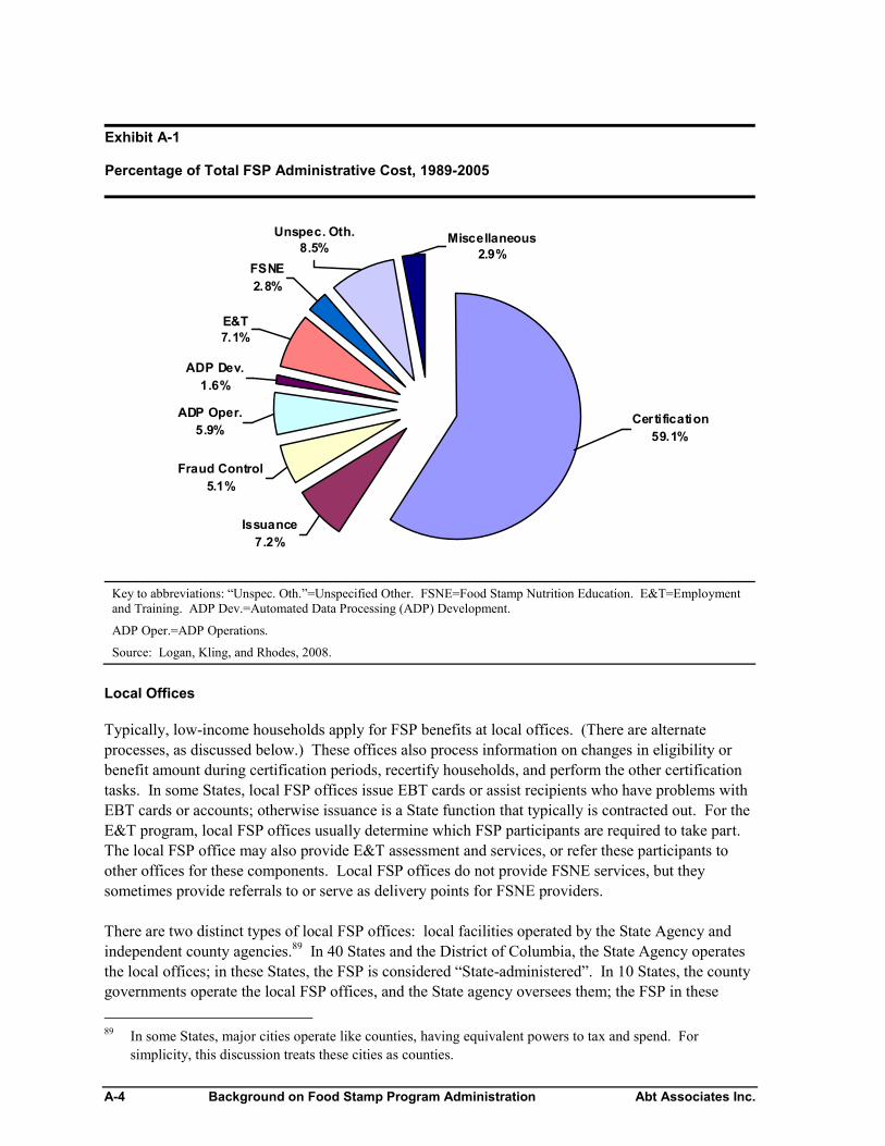
A-4 Background on Food Stamp Program Administration Abt Associates Inc.
Exhibit A-1
Percentage of Total FSP Administrative Cost, 1989-2005
Certification59.1%
Issuance7.2%
Fraud Control5.1%
ADP Oper.5.9%
ADP Dev.1.6%
E&T7.1%
FSNE2.8%
Unspec. Oth.8.5%
Miscellaneous2.9%
Key to abbreviations: “Unspec. Oth.”=Unspecified Other. FSNE=Food Stamp Nutrition Education. E&T=Employmentand Training. ADP Dev.=Automated Data Processing (ADP) Development.
ADP Oper.=ADP Operations.
Source: Logan, Kling, and Rhodes, 2008.
Local Offices
Typically, low-income households apply for FSP benefits at local offices. (There are alternateprocesses, as discussed below.) These offices also process information on changes in eligibility orbenefit amount during certification periods, recertify households, and perform the other certificationtasks. In some States, local FSP offices issue EBT cards or assist recipients who have problems withEBT cards or accounts; otherwise issuance is a State function that typically is contracted out. For theE&T program, local FSP offices usually determine which FSP participants are required to take part.The local FSP office may also provide E&T assessment and services, or refer these participants toother offices for these components. Local FSP offices do not provide FSNE services, but theysometimes provide referrals to or serve as delivery points for FSNE providers.
There are two distinct types of local FSP offices: local facilities operated by the State Agency andindependent county agencies.89 In 40 States and the District of Columbia, the State Agency operatesthe local offices; in these States, the FSP is considered “State-administered”. In 10 States, the countygovernments operate the local FSP offices, and the State agency oversees them; the FSP in these
89 In some States, major cities operate like counties, having equivalent powers to tax and spend. Forsimplicity, this discussion treats these cities as counties.
Abt Associates Inc. Background on Food Stamp Program Administration A-5
States is “State-supervised, county-administered”.90 Local office employees—who represent thelargest cost in administering the FSP—are employed by the State or county, whichever leveladministers the local level. Where the FSP is State-supervised and county-administered, there aretwo levels of government involved, each with its own elected officials, management, appropriations,accounting system, and personnel system.
State Food Stamp Agency and Other Organizations
The role of the State Food Stamp Agency depends on whether the State Agency directly administersthe FSP at the local level, but there are roles that are common to all States. First, State Agenciesprovide policy direction and oversight to all aspects of FSP administration, including those involvingcounties and service providers (which may be other government agencies or private contractors).Second, State Agencies contract with service providers to operate their EBT issuance systems and toprovide E&T and FSNE. Third, State Agencies develop and operate ADP systems for the FSP, eitherin-house or with support from service providers. Fourth, State Agencies carry out mandatory supportfunctions, including fair hearings, quality control, and management evaluation.
The role of the State Agency varies across States in several ways.
As noted, most State Agencies directly administer certification and other functions of localoffices, while a minority supervises county agencies performing these functions.
Some State Agencies operate call centers or websites that provide alternative interfaces withcustomers for providing information, submitting FSP applications, reporting householdchanges, recertification, troubleshooting, or other interactions (APHSA, 2006).
Some State Agencies establish agreements with private voluntary organizations that assistFSP applicants with initial applications and other certification activities (GAO, 2007).
Some State Agencies operate their own ADP facilities (including computer centers andnetworks) and maintain their own software, while others contract these functions out tocentralized State support agencies (e.g., Department of Administration) or to private firms.Similarly, development of ADP systems may be in-house, outsourced, or a combination ofthese approaches.
90 Counts provided via personal communication with FNS.

A-6 Background on Food Stamp Program Administration Abt Associates Inc.
Abt Associates Inc. Accountability and Reporting of Expenditures B-1
Appendix B
Accountability and Reporting of State FSPAdministrative Expenditures
The process of determining State administrative expenses (SAE) for the FSP is complex. First, Statesmust record all of their administrative expenditures (payroll, purchases, interagency transfers, etc.) forthe FSP and other programs following standard government accounting procedures. Second, Statesmust determine the expenditures allocable to each program. Many expenditures that benefit the FSPalso benefit other programs. FSP workers often work on other public assistance programs (e.g.,TANF, Medicaid, State cash benefit programs, etc.). Supervisors and administrators—from officedirectors up through the highest level of State bureaucracies—also work on multiple programs.Further, nonlabor expenditures—data processing, facilities, supplies, etc.—also support multipleprograms. In order to determine expenditures for the FSP, States need methods to allocate the costsof such shared resources between the programs that benefit from the expenditures. Finally, once SAEfor the FSP has been determined, the State must report the expenses to FNS in a standard format, withexpenses broken down by program function (of which the largest is certification).
This appendix discusses how States deal with these challenges. Understanding what States do iscrucial for understanding what data are available and their quality. First, we summarize theframework of rules and oversight for reporting of SAE. Next, we note the role of accounting systemsin the SAE determination process. In the following section, we review the basic methods forallocating expenses to the FSP. Then, we describe typical costs and allocation methods for each ofthe major types of FSP administrative activities: local agency operations, other client services, dataprocessing and telecommunications, program oversight and support, and general administration(within the State Food Stamp Agency and statewide). We conclude with a brief description of theSAE reports submitted to FNS.
As noted in Chapter One, this report is based on interviews with Federal officials and with officials infour States. Thus, the description does not necessarily apply in detail to all States. However, ourinformation is sufficient for a broad overview to provide background to the discussion in the report onthe comparability and usefulness of data from the administrative cost accounting and allocationprocesses for studies of variation in SAE.
The discussion in this report is generally framed in terms of what States do. In 40 of the 50 Statesand in the District of Columbia, the State government (or its equivalent) administers the FSP.However, county governments administer the FSP under State supervision in 10 States, including oneof the four included in this study. In these States, the counties measure and allocate FSPadministrative expenses, and submit claims to the State for reimbursement. The State then combinesthe county expenses and its own administrative expenses, and reports the State total to FNS. For easeof discussion, we describe cost allocation as conducted where the FSP is State-administered. Formost aspects of cost reporting, the methods and issues are the same across these two structures for theFSP. We do, however, note and discuss how cost allocation is different where the FSP is county-administered and State-supervised.
B-2 Accountability and Reporting of Expenditures Abt Associates Inc.
Allowable Expenditures
The Food Stamp Act (P.L. 93-347, as amended) authorizes the U.S. Department of Agriculture(USDA) to pay half of all States’ costs for administering the program and requires “efficient andeffective administration” by the States. Allowable costs are carefully spelled out in Federalregulations (see Title 7/Agriculture, Part 277/Payments of Certain Administrative Costs of StateAgencies). The basic principles are laid out in Appendix A to 7:277/Principles for Determining CostsApplication to Administration of the Food Stamp Program by State Agencies. Specifically, the“fundamental premises” are (A:2):
(a) State agencies are responsible for the efficient and effective administration of the FoodStamp Program through the application of sound management practice.
(b) The State agency assumes the responsibility for seeing that Food Stamp Program fundshave been expended and accounted for consistent with underlying agreements andprogram objectives.
(c) Each State agency, in recognition of its own unique combination of staff facilities andexperience, will have the primary responsibility for employing whatever form oforganization and management techniques as may be necessary to assure proper andefficient administration.
There are two phases of Federal oversight of SAE. Before funds are expended, State Agencies arerequired to submit their SAE budgets to FNS for prior approval (7 CFR 272.2). Then, afterexpenditures are reported, they are reviewed periodically by FNS and included in the State Agencies’organization-wide audits conducted under instructions from the Office of Management and Budget(OMB Circular A-133). In practice, under the third fundamental principle, State Agencies havesubstantial latitude in designing their FSP administrative systems and in allocating resources. StateAgencies are required to justify major year-to-year changes in their budgets for operations, and theymust provide detailed justification of ADP development budgets. On the other hand, the StateAgencies are not required to provide a bottom-up justification of their operating budgets inrelationship to the caseload they expect to serve and the functions required to administer thiscaseload. Preliminary information from discussions with FNS officials suggests that, in practice, theyhave limited scope to question actual expenditures. FNS oversight appears to focus on whether costsare adequately documented and correctly allocated, and whether prior approval was obtained ifrequired.
Accounting Systems and Controls
States use their accounting systems to record the funds appropriated for administering their programsand the disbursements of these funds. Thus, the most fundamental data underlying State reports ofSAE are the transactions for payments to employees, contractors, suppliers, and other agencies for thegoods and services that enable the programs to operate.
For this feasibility study, we have assumed that the goal of future studies will be to explain variationin actual reported FSP administrative expenses. While there may be economic costs that are notidentified under government accounting rules, such as the value of uncompensated overtime byexempt workers, we have disregarded this aspect of administrative costs.
Abt Associates Inc. Accountability and Reporting of Expenditures B-3
We have further assumed, as a necessary and useful simplification, that this study is not concernedwith the possibility that actual administrative expenditures may occasionally include errors indisbursements (underpayments or overpayments). Control of disbursements is a fundamentalresponsibility of State accounting systems and officials, and disbursements are subject to State andFederal audits and other oversight. None of the discussions in the interviews suggested that errors indisbursements might materially and systematically affect the variation in reported expenses. Wehave, therefore, focused our investigation on the factors that may introduce error in the allocation andreporting of the actual disbursements. Error in this context includes any difference between the actualreported expenses and what the State would report if the actual disbursements were allocated andreported in a way that accurately reflects the use of the disbursed funds.
Methods for Allocating Expenses to the FSP
There are three basic ways that States allocate expenses to the FSP: direct charges, allocation basedon usage, and allocation in proportion to usage of other resources. Below, we briefly describe each ofthese basic methods, which are explained in more detail in subsequent sections.
Expenses that are exclusively attributable to the FSP are directly charged in the accounting system.Compensation for local or State staff who work only on the FSP is one type of expense that may bedirectly charged; materials for FSP outreach (posters etc.) and payments to EBT vendors for benefitissuance represent other examples.
Shared expenses for the FSP and other programs may be allocated in proportion to usage. Forpersonnel costs, a time measurement system is used. One type of time measurement is periodic timereporting (timesheets); in this method, specified personnel record all of their time on a continuousbasis, including program-specific time, joint time for two or more programs, and nonspecific time(breaks, leave, general meetings, etc.). The other main method for measuring staff time acrossprograms is a random-moment time study (RMTS), in which randomly selected personnel recordwhat they are doing at randomly selected moments, and the distribution of moments is used toestimate the overall distribution of time for the specified population of personnel. Computer usagemay be monitored in various ways: processing units, storage space, pages printed, etc. Once theusage of a resource for all programs is determined, each program’s cost is computed.
Finally, shared expenses may be allocated in proportion to usage of other resources. This methodis used for expenses for which it is infeasible or disproportionately burdensome to determine usage bythe FSP and other programs. For example, costs associated with operating and maintaining facilitiescannot readily be allocated in proportion to usage, because activities for more than one program canoccur in the same space. Facility costs could be allocated simply in proportion to the distribution ofstaff time across programs or alternatively in proportion to the costs allocated through the other twomethods (direct charges and in proportion to usage).
The choices among these cost allocation methods are governed by Federal rules. Each State mustestablish a Public Assistance Cost Allocation Plan (PACAP) to specify how it determines the coststhat will be charged to the FSP, TANF, Medicaid, and other Federal “public assistance” programs.The PACAP identifies all of the activities or functions performed by the State agency, the types ofcosts associated with these activities and functions, the programs that benefit, and how costs arecharged or allocated to these programs. Groups of related costs that are allocated the same way are
B-4 Accountability and Reporting of Expenditures Abt Associates Inc.
defined as “cost pools”. (For example, the State’s fraud investigation unit could be a cost pool, withpersonnel and nonpersonnel costs allocated in proportion to the number of investigations for eachprogram.) In addition, the State must have a Statewide Cost Allocation Plan to specify how statewideadministrative costs (such as centralized services, audits, purchasing, etc.) are allocated acrossagencies and programs. Counties that claim Federal funding must have their own cost allocationplans. The cost allocation plans must meet the principles of OMB Circular A-87. The Department ofHealth and Human Services, Division of Cost Allocation (DCA), issues additional guidelines forPACAPs (HHS, 1997 and HHS, 2002). Both DCA and FNS review cost allocation plan wheneverthey are changed. In addition, FNS reviews actual expenses to determine (among other things)whether States are following their cost allocation plans. Cost allocation plans contain a considerableamount of information about State agencies’ activities, organizational units, and types of costs, andthus these documents represent a potential resource for research on SAE.
States use several methods to allocate local office costs for the FSP. In the following section, wedescribe the methods used to allocate local labor and nonlabor costs.
Local Office Costs
Local office costs are the largest component of FSP administrative expenses, and workers dealingdirectly with customers are the largest component of local office costs (HHS, 2002). In theconventional approach to FSP administration, local offices of the State Food Stamp Agency conductall certification activities (intake, case maintenance, recertification, etc.).91 Local offices may also beinvolved in Food Stamp Employment and Training (E&T) functions. These E&T functions mayinclude eligibility-related roles (determining which participants are subject to E&T requirements andwhether they are complying, and applying sanctions); in some States, local offices also operateprogram components such as supervised job search. Local staff may have roles in fraud control, suchas establishing claims for overpayments, and in some functions for electronic benefit transfer (EBT)systems (issuing EBT cards, training recipients, etc.).
Local offices usually administer eligibility for FSP, TANF and Medicaid, and often for otherprograms, such as State cash and medical assistance programs, and the Low Income Heating andEnergy Assistance Program (LIHEAP). In some States, these “income maintenance” or “publicassistance” functions are collocated with social services (e.g., child protective services), child supportenforcement, or employment services and workforce development. Collocated programs sharefacilities and may also share a local office director and general administrative staff (personnel office,mailroom, finance and accounting, information technology, etc.).
Some local office workers specialize in a single program, while others serve multiple programs.Local offices may have varying mixes of single-program and multi-program or “generalist” workers.In three of the four States interviewed, most or all FSP eligibility workers also serve other programs.In North Carolina, most FSP eligibility workers do not serve other programs, but a minority do, andadministrative and support staff are shared between the FSP and other programs, as well as facilities,office equipment, supplies, and other non-personnel resources.
91 As discussed elsewhere in this report, some States use call centers to perform certification functions that donot require face-to-face contact.
Abt Associates Inc. Accountability and Reporting of Expenditures B-5
The States use multiple methods to allocate local office costs for the FSP. In the following sections,we describe the methods used to allocate labor and nonlabor costs.
Local Labor Costs
The methods for allocating local labor costs are particularly important. According to all of the Stateswe spoke to, local labor costs represent the largest component of FSP administrative costs. Inaddition, the distribution of local staff time or labor costs is often used to allocate other costs, such aslocal nonlabor costs or State-level labor costs. For these reasons, the methods for allocating locallabor costs have a major influence on the overall accuracy and consistency of FSP expenditurereporting. At the same time, data on local labor costs from the accounting process represent animportant potential source of insights into overall variation in FSP SAE.
For personnel costs, the starting point in the allocation process is payroll records. Payroll recordsindicate the amount paid to staff during each accounting period, and the cost pools to which thecompensation is charged (including salaries and benefits).
The simplest case is the allocation of costs for staff members who work only on the FSP. Theircompensation is charged directly to a FSP cost pool. These staff must certify semi-annually that thatthey work only on the FSP. Most offices in North Carolina have separate units for the FSP, however,so the workers complete semi-annual effort certifications. For these workers, no detailed timereporting system is needed for cost allocation.
Allocating the cost of staff members who work on more than one program is more complicated. Suchstaff members include multi-program eligibility workers, support staff, supervisors, and managers.For these personnel, compensation is charged to one or more shared cost pools. For multi-programeligibility workers, the cost pool is then allocated among programs using one of two approved timereporting methods: random-moment time studies or personnel activity reports.
The HHS Division of Cost Allocation (DCA) recommends random-moment time studies (RMTS),and most States (including Nevada, New Mexico, and Pennsylvania) use this method for most or allof their eligibility workers. (Some States include other income maintenance workers who have directclient contact in their RMTS.) The State constructs a sample frame of eligibility workers and theirschedules, then selects “worker moments” (i.e., worker X at time Y on date Z) using a randomsampling algorithm. For each sampled “worker moment”, the selected worker is required to reportwhat he or she is doing, including: the program or program combination served, the case number orname of the client, and sometimes a code indicating the general type of activity (initial application,change, recertification, etc.). If the worker is not serving a client or otherwise working on a specificprogram, then only the activity is recorded (break, leave, general meetings, etc.). The DCA hasestablished a minimum statewide sample of 2,000 valid RMTS observations per quarter; States needto sample additional observations because there are always some that are not completed and valid.(For example, the worker may not be actually scheduled to work at the sampled moment.) The Statetabulates the percentage of observations for each program and program combination, and uses thesepercentages to allocate the total compensation cost for all of the eligibility workers, including thosewho had moments sampled in the quarter and those who did not.
Under the personnel activity reporting method, each worker reports all activity during a month orshorter period, indicating the program or programs served and, for activities involving individual
B-6 Accountability and Reporting of Expenditures Abt Associates Inc.
clients, the name or case number. Local social service offices in North Carolina use this method,albeit for relatively few FSP workers (due to the predominance of separate FSP units). Multi-program eligibility workers and social service workers complete daily records of client contacts andother activities, and then complete a monthly summary of time by program or program combination.These data are used to allocate the workers’ compensation to the FSP and other programs.
States generally use the time-reporting data from eligibility workers when they allocate local laborcosts for support staff, supervisors, and managers, but there are different approaches.
Some States use the percentage of eligibility worker time by program from a RMTS toallocate all local labor costs. In these States, the RMTS covers all eligibility workers and allprograms operated by the local offices.
Other States combine RMTS or personnel activity reports with effort certifications todetermine the percentage of full-time equivalent eligibility workers for each program. Then,the State applies these percentages to allocate the other local labor costs.
Finally, some States use the distribution of eligibility worker costs and nonlabor costscharged directly to specific programs to determine percentages for each program. Thesepercentages are then used to allocate the rest of the local labor cost (and possibly some sharednonlabor costs) in proportion to the cost already allocated. Depending on the State, thedistribution of eligibility worker costs may be based on RMTS, personnel activity reports,effort certifications, or some combination of these methods.
Allocation of local labor costs is sometimes a multi-stage process. In the first stage, compensation forgeneral managers and their support staff is allocated to local office divisions (e.g., social services andincome maintenance) in proportion to the number of staff in each division. In the second stage, thetotal compensation for each division, including the allocated general management and support, isallocated among the programs served by the division in proportion to the percentage of time foreligibility workers and other workers who report time by program.
Local Nonlabor Costs
In principle, the nonlabor costs of operating local offices include all of the resources used by localpersonnel: supplies, facilities, equipment, telecommunications, data processing systems, postage anddelivery, and other contracted services. In practice, States vary with regard to which of theseresources are treated as local agency costs and which are part of some other pool of costs. In county-administered States, such as North Carolina, county departments are responsible for all of these costs,except for statewide data processing systems and associated networks. Counties may have their owndata processing expenses. For example, some counties in North Carolina have automated systemsthat supplement the capabilities of the statewide client information system for the FSP. Where theFSP is State-administered, some or most goods and services for local offices may be purchasedcentrally and treated as a State-level cost assigned to the income maintenance division or a generaladministrative division.
The approaches to allocating local nonlabor costs are similar to those for allocating local labor costsother than compensation for eligibility workers and other personnel with direct client contact. Somelocal nonlabor costs are charged directly to a program. Shared costs are allocated in proportion to theRMTS time percentages, total staff time, or total costs charged on the basis of time use or direct
Abt Associates Inc. Accountability and Reporting of Expenditures B-7
charges. A step-down process may be used where nonlabor costs such as rent and utilities are firstallocated among divisions within local offices (based on FTEs or some other factor), then amongprograms within divisions.
State Costs
State agencies typically operate data processing and telecommunications systems to support eligibilitydetermination, case maintenance, and other program functions. In addition, State agencies operate orcontract for client services not provided by local offices, including benefit issuance, nutritioneducation, and employment and training. Finally, State agencies disseminate policy, provide training,and perform oversight functions (including quality control and management evaluation). As withlocal costs, cost allocation methods include direct charges, allocation based on usage, and allocationbased on other costs.
Data Processing and Telecommunications
This category includes a variety of costs associated with client information systems, othermanagement information and accounting systems, computer networks, and voice communications.The principal types of costs include: State technical personnel, contractors and service providers,equipment, software, and facilities. (Facility costs include rent or depreciation, utilities, cleaning, andmaintenance of building systems.) These resources are shared among income maintenance programsand often with other programs within the same department. In some States, there is a centralinformation technology department that operates a statewide computer center, data network, or both,serving most or all State agencies.
A variety of methods are used to charge data processing and telecommunications costs to the FSP.State personnel and contractors working on development and maintenance of computer applicationsand databases typically maintain activity reports (timesheets), with time tracked by project and aspecified percentage of costs for each project allocated to one or more programs. The allocationpercentage may be based on an indicator of usage or caseload, or based on a determination of howmuch of the project benefits each program (e.g., number of lines of program code). Computer systemusage may be tracked at the program/program combination level, so that the operating costs for thesystem can be allocated in proportion to usage, or so that previously established charges can beassessed for each unit of usage. These operating costs may be “all-in” (inclusive of all expenses tooperate the facility) or a subset of expenses. Alternatively, a pool of computer system costs forincome maintenance programs (possibly including telecommunications network costs) may beallocated in proportion to the RMTS percentages for local personnel. Finally, percentages of costsallocated by other means may be used to allocate data processing and telecommunications costs.
Client Services
States frequently contract out three types of FSP client services: EBT, nutrition education, and E&T.EBT is almost universally provided by contractors on a fee-for-service basis. No cost allocationissues are raised. The contractor bills separately for services to the FSP and, where applicable, forother programs (as in the case of EBT, which also delivers cash benefits in some States). Nutritioneducation (FSNE) and E&T are often contracted out to other State or county agencies, and theseservices also are directly charged to the FSP. The State or county agency providing FSNE must,
B-8 Accountability and Reporting of Expenditures Abt Associates Inc.
however, use cost allocation methods that comply with Circular A-87 in determining their claims forreimbursement from the State Food Stamp Agency.
In addition, some States operate call centers or other centralized operations to supplement or replaceservices otherwise provided at the local level. These centers may be simply information and referralservices, or they may perform certification functions such as change reporting or recertification.Methods for allocating the costs for call centers and other centralized client services include calltracking by program, RMTS, use of local RMTS percentages, and allocation based on percentages ofcosts allocated by other means.
Policy, Program Oversight, and Statewide Administration
Other State costs include FSP-specific activities, joint income maintenance administration, andgeneral administration within and outside the State agency. FSP-specific activities, such as policyand training, may be directly charged. Some joint income maintenance administrative activities maybe charged on the basis of activity counts for the FSP and other programs; this method may be usedfor quality control reviews (done for FSP and Medicaid), fair hearings, and fraud investigations.Alternatively, State personnel maintain activity reports as the basis for allocating their time. Thedistribution of local staff time or costs may be used to allocate shared State administrative costs forwhich personnel activity reports are not feasible. Cost allocation plans may have multi-step processesfor allocating general State agency administrative costs (management, personnel, accounting, etc.)and the agency’s share of statewide administrative costs. As at the local level, such costs may beallocated among divisions by FTEs or another equitable basis, and then within divisions by programbased on available allocation factors (percentage of time or costs, etc.).
Reporting of Food Stamp Administrative Expenses to FNS
State Agencies submit quarterly and annual reports of FSP administrative expenses to FNS on the SF-269 report. The report is organized in columns representing specific program functions, such ascertification, benefit issuance, and automated data processing (ADP). For each column, the Statereport identifies Federal and non-Federal shares of outlays. (The SF-269 form is shown at the end ofthis appendix.)
States use a combination of methods to determine the portion of FSP administrative expenses thatthey report in each functional category on the SF-269. It appears that most types of expenses aregrouped in cost centers or pools that are associated with a single FSP function. For example, separatecost pools can be defined for the units that perform quality control reviews, fraud investigations, fairhearings, and management evaluations. Some cost centers or pools serve more than one FSPfunction, so additional data are needed to separate the costs by function. Eligibility workerssometimes perform both certification and employment and training (E&T) functions; States useRMTS or personnel activity reports to track these activities separately for cost reporting. Similarly,programmers may work on both ADP system maintenance (an operational expense) and developmentof a new ADP system. The State has to have a mechanism, such as personnel activity reports, toallocate time between ADP operations and development, because only time on approved projects canbe charged to the ADP development category. Finally, some overhead-type expenses (e.g., a portionof the State Agency’s senior management costs) are allocated among organizational units and, as aresult, spread over several functions. The supporting documentation for the SF-269 documents howthe costs for each function are computed and what cost centers or pools are included.
Abt Associates Inc. Accountability and Reporting of Expenditures B-9
The Federal share (also known as Federal Financial Participation, or FFP) is set by law at 50 percentof reimbursable expenses, with some exceptions. States receive a base grant of 100 percent Federalfunds for E&T; additional expenses are reimbursed at 50 percent. Under the Quality Control (QC)sanctions rules, State Agencies are allowed to “reinvest” their own funds in FSP improvements, ratherthan pay sanctions for excessive error rates. Reinvested funds are reported separately from regularexpenditures, and FNS does not match these expenditures.92 Prior to 1994, FNS provided enhancedfunding for several categories of expenditures, with the Federal share between 63 and 100 percent.93
Starting in FY1999, the Federal share of certification costs has been reduced to offset the FSP shareof common costs included in each State’s TANF grant, as required by the Agricultural Research,Extension, and Education Reform Act of 1998 (P.L. 105-185). At the time of this legislation, therewas concern that States would shift costs from their fixed TANF grants to the FSP, which has open-ended Federal matching funds for administration (Carmody and Dean, 1998). Under the law, theDepartment of Health and Human Services (HHS) was required to analyze the allocation of sharedcosts between the FSP and Aid to Families with Dependent Children (AFDC, the predecessor toTANF) during the baseline period used to set levels for States’ TANF grants. The law required FNSto withhold a portion of Federal reimbursements for FSP certification costs to offset FSP-related coststhat had been included in State AFDC administrative costs and therefore were included in StateTANF grants that were based on the AFDC costs. HHS determined that some States had substantialamounts of these former AFDC costs that were attributable to joint certification of AFDC/FSP cases,while others had little or no such costs (Goolsby, 2004).
States also report Federal and non-Federal shares of unliquidated obligations for each function on theSF-269. Unliquidated obligations represent commitments of funds that have not been formallyexpended (i.e., liquidated). The liquidation of obligations is part of the process of finalizingexpenditures for a fiscal year. States are allowed to claim additional Federal reimbursement fromobligated funds for up to two years after the end of a fiscal year. Thus, Federal expenditures for afiscal year are not final until at least two years later, and may be revised even later on the basis of aState audit or a Federal review of expenditures.
The SF-269 form and the definitions of the reporting categories from FNS instructions appear on thefollowing pages.
92 Sanctions and bonuses based on QC error rates are not reported as part of SAE. Prior to implementation ofthe 2002 Farm Bill, States with payment error rates below 5.9 percent received enhanced funding. Underthe QC reforms of the 2002 Farm Bill, FNS awards bonuses of $48 million per year on the basis of high orimproved performance in payment error rates, timeliness, and the Program Access Index.
93 ADP development was reimbursed at 75 percent through FY1991, then at 63 percent through March 1994.Systematic Alien Verification of Eligibility system costs were reimbursed at 100 percent through March1994. Fraud control costs were reimbursed at 75 percent through March 1994. Expenses for administeringthe FSP on Indian Reservations are currently reimbursed at 75 percent.

FORM APPROVED OMB NO. 0348-0039
FINANCIAL STATUS REPORT1. FEDERAL AGENCY & ORGANIZATIONAL ELEMENT TO WHICH REPORT IS SUBMITTED
FEDERAL GRANT OR OTHERNUMBER 2a. FISCAL YEAR
FOOD AND NUTRITION SERVICE, USDA Letter of CreditNo. 12-35-
3. RECIPIENT ORGANIZATION (Name and complete address, includingZIP code. Also enter assigned State code.)
4. UNIVERSAL IDENTIFIER NUMBER 5. RECIPIENT ACCOUNT NUMBER ORIDENTIFYING NUMBER
6. FINAL REPORT 7. BASIS
___CASH ___ ACCRUAL
8. PROJECT/GRANT PERIOD 9. PERIOD COVERED BY THIS REPORT
10. STATUS OF FUNDS FOOD STAMP PROGRAM1 2 3 4 5 6 7 8 9 10
PROGRAMS/FUNCTIONS/ACTIVITIES CERTIFICATION COUPON PERFORMANCE REPORTING 50% FUNDING 75% FUNDING ADP OPER FAIR OTHER TOTAL
ISSUANCE QUAL. CNTL. MGT.EVAL. FRAUD CNTL. FRAUD CNTL. HEARINGS ACTIVITIES
a. Net outlays previously reported
b. Total outlays this report period
c. Less: Program Income credits
d. Net outlays this report period(Line b minus line c)
e. Net outlays to date(Line a plus line d)
f. Less: Non-Federal share of outlays
g. Total Federal share of outlays(Line e minus line f)
h. Total unliquidated obligations
i. Less: Non-Federal share of unliquidatedobligations shown on line h
j. Federal share of unliquidated obligations
k. Total Federal share of outlaysand unliquidated obligations
l. Total cumulative amount of Federalfunds authorized
m. Unobligated balance of Federal funds
11. INDIRECT
a. TYPE OF RATE___PROVISIONAL ___ PREDETERMINED ___ FINAL ___ FIXED
13. CERTIFICATION SIGNATURE OF AUTHORIZEDCERTIFYING OFFICIAL
DATE REPORT SUBMITTED
EXPENSE b. RATE c. BASE d. TOTAL AMOUNT e. FEDERAL SHARE I certify to the best of my knowledge and belief thatthis report is correct and complete and that alloutlays and unliquidated obligations are for thepurposes set forth in the award documents.12. REMARKS: Attach any explanation deemed necessary or information required by Federal sponsoring agency in
compliance with governing legislation.
STAMP DATE LAST UPDATED BY LAST UPDATED ON NAME TITLE TELEPHONE NO.AREA CODE NUMBER
-
No further monies or other benefits may be paid out under this program unless this NOTE: When reordering this form specify "SF-269 FOOD STAMP " STANDARD FORM 269 (7-03) (FOOD STAMP)report is completed and filed as required by existing regulation (34 C.F.R 256) Exception to SF-269. approved by NARS (11-80) Printed onNDB Electronic Version Page 1 of 4
Page 1 of 4
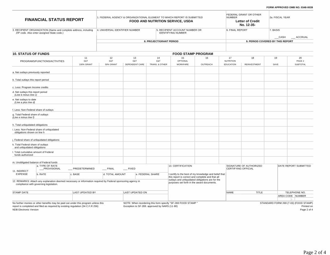
FORM APPROVED OMB NO. 0348-0039
FINANCIAL STATUS REPORT1. FEDERAL AGENCY & ORGANIZATIONAL ELEMENT TO WHICH REPORT IS SUBMITTED
FEDERAL GRANT OR OTHERNUMBER 2a. FISCAL YEAR
FOOD AND NUTRITION SERVICE, USDA Letter of CreditNo. 12-35-
3. RECIPIENT ORGANIZATION (Name and complete address, includingZIP code. Also enter assigned State code.)
4. UNIVERSAL IDENTIFIER NUMBER 5. RECIPIENT ACCOUNT NUMBER ORIDENTIFYING NUMBER
6. FINAL REPORT 7. BASIS
___CASH ___ ACCRUAL
8. PROJECT/GRANT PERIOD 9. PERIOD COVERED BY THIS REPORT
10. STATUS OF FUNDS FOOD STAMP PROGRAM11 12 13 14 15 16 17 18 19 20
PROGRAMS/FUNCTIONS/ACTIVITIES E&T E&T E&T E&T OPTIONAL NUTRITION PAGE 2
100% GRANT 50% GRANT DEPENDENT CARE TRANS. & OTHER WORKFARE OUTREACH EDUCATION REINVESTMENT SAVE SUBTOTAL
a. Net outlays previously reported
b. Total outlays this report period
c. Less: Program Income credits
d. Net outlays this report period(Line b minus line c)
e. Net outlays to date(Line a plus line d)
f. Less: Non-Federal share of outlays
g. Total Federal share of outlays(Line e minus line f)
h. Total unliquidated obligations
i. Less: Non-Federal share of unliquidatedobligations shown on line h
j. Federal share of unliquidated obligations
k. Total Federal share of outlaysand unliquidated obligations
l. Total cumulative amount of Federalfunds authorized
m. Unobligated balance of Federal funds
11. INDIRECT
a. TYPE OF RATE___PROVISIONAL ___ PREDETERMINED ___ FINAL ___ FIXED
13. CERTIFICATION SIGNATURE OF AUTHORIZEDCERTIFYING OFFICIAL
DATE REPORT SUBMITTED
EXPENSE b. RATE c. BASE d. TOTAL AMOUNT e. FEDERAL SHARE I certify to the best of my knowledge and belief thatthis report is correct and complete and that alloutlays and unliquidated obligations are for thepurposes set forth in the award documents.12. REMARKS: Attach any explanation deemed necessary or information required by Federal sponsoring agency in
compliance with governing legislation.
STAMP DATE LAST UPDATED BY LAST UPDATED ON NAME TITLE TELEPHONE NO.AREA CODE NUMBER
-
No further monies or other benefits may be paid out under this program unless this NOTE: When reordering this form specify "SF-269 FOOD STAMP " STANDARD FORM 269 (7-03) (FOOD STAMP)report is completed and filed as required by existing regulation (34 C.F.R 256) Exception to SF-269. approved by NARS (11-80) Printed onNDB Electronic Version Page 2 of 4
Page 2 of 4

FORM APPROVED OMB NO. 0348-0039
FINANCIAL STATUS REPORT1. FEDERAL AGENCY & ORGANIZATIONAL ELEMENT TO WHICH REPORT IS SUBMITTED
FEDERAL GRANT OR OTHERNUMBER 2a. FISCAL YEAR
FOOD AND NUTRITION SERVICE, USDA Letter of CreditNo. 12-35-
3. RECIPIENT ORGANIZATION (Name and complete address, includingZIP code. Also enter assigned State code.)
4. UNIVERSAL IDENTIFIER NUMBER 5. RECIPIENT ACCOUNT NUMBER ORIDENTIFYING NUMBER
6. FINAL REPORT 7. BASIS
___CASH ___ ACCRUAL
8. PROJECT/GRANT PERIOD 9. PERIOD COVERED BY THIS REPORT
10. STATUS OF FUNDS FOOD STAMP PROGRAM21 22 23 24 25 26 27 28 29 30
PROGRAMS/FUNCTIONS/ACTIVITIES 50% FUNDING 63% FUNDING 75% FUNDING EBT ISSUANCE EBT UNSPECIFIED E&T PAGE 3
ADP DEV. ADP DEV. ADP DEV. ISSUANCE INDIRECT STARTUP PORTION OF OTHER ABAWD GRANT SUBTOTAL
a. Net outlays previously reported
b. Total outlays this report period
c. Less: Program Income credits
d. Net outlays this report period(Line b minus line c)
e. Net outlays to date(Line a plus line d)
f. Less: Non-Federal share of outlays
g. Total Federal share of outlays(Line e minus line f)
h. Total unliquidated obligations
i. Less: Non-Federal share of unliquidatedobligations shown on line h
j. Federal share of unliquidated obligations
k. Total Federal share of outlaysand unliquidated obligations
l. Total cumulative amount of Federalfunds authorized
m. Unobligated balance of Federal funds
11. INDIRECT
a. TYPE OF RATE___PROVISIONAL ___ PREDETERMINED ___ FINAL ___ FIXED
13. CERTIFICATION SIGNATURE OF AUTHORIZEDCERTIFYING OFFICIAL
DATE REPORT SUBMITTED
EXPENSE b. RATE c. BASE d. TOTAL AMOUNT e. FEDERAL SHARE I certify to the best of my knowledge and belief thatthis report is correct and complete and that alloutlays and unliquidated obligations are for thepurposes set forth in the award documents.12. REMARKS: Attach any explanation deemed necessary or information required by Federal sponsoring agency in
compliance with governing legislation.
STAMP DATE LAST UPDATED BY LAST UPDATED ON NAME TITLE TELEPHONE NO.AREA CODE NUMBER
-
No further monies or other benefits may be paid out under this program unless this NOTE: When reordering this form specify "SF-269 FOOD STAMP " STANDARD FORM 269 (7-03) (FOOD STAMP)report is completed and filed as required by existing regulation (34 C.F.R 256) Exception to SF-269. approved by NARS (11-80) Printed onNDB Electronic Version Page 3 of 4
Page 3 of 4
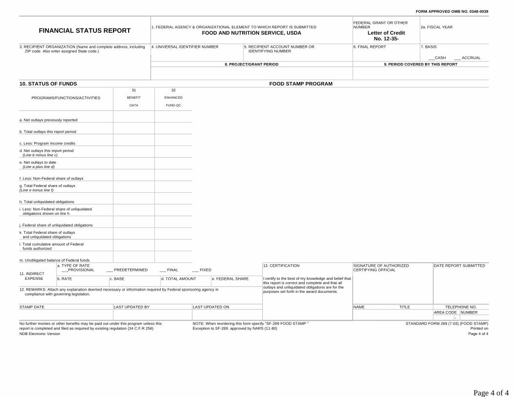
FORM APPROVED OMB NO. 0348-0039
FINANCIAL STATUS REPORT1. FEDERAL AGENCY & ORGANIZATIONAL ELEMENT TO WHICH REPORT IS SUBMITTED
FEDERAL GRANT OR OTHERNUMBER 2a. FISCAL YEAR
FOOD AND NUTRITION SERVICE, USDA Letter of CreditNo. 12-35-
3. RECIPIENT ORGANIZATION (Name and complete address, includingZIP code. Also enter assigned State code.)
4. UNIVERSAL IDENTIFIER NUMBER 5. RECIPIENT ACCOUNT NUMBER ORIDENTIFYING NUMBER
6. FINAL REPORT 7. BASIS
___CASH ___ ACCRUAL
8. PROJECT/GRANT PERIOD 9. PERIOD COVERED BY THIS REPORT
10. STATUS OF FUNDS FOOD STAMP PROGRAM31 32
PROGRAMS/FUNCTIONS/ACTIVITIES BENEFIT ENHANCED
DATA FUND-QC
a. Net outlays previously reported
b. Total outlays this report period
c. Less: Program Income credits
d. Net outlays this report period(Line b minus line c)
e. Net outlays to date(Line a plus line d)
f. Less: Non-Federal share of outlays
g. Total Federal share of outlays(Line e minus line f)
h. Total unliquidated obligations
i. Less: Non-Federal share of unliquidatedobligations shown on line h
j. Federal share of unliquidated obligations
k. Total Federal share of outlaysand unliquidated obligations
l. Total cumulative amount of Federalfunds authorized
m. Unobligated balance of Federal funds
11. INDIRECT
a. TYPE OF RATE___PROVISIONAL ___ PREDETERMINED ___ FINAL ___ FIXED
13. CERTIFICATION SIGNATURE OF AUTHORIZEDCERTIFYING OFFICIAL
DATE REPORT SUBMITTED
EXPENSE b. RATE c. BASE d. TOTAL AMOUNT e. FEDERAL SHARE I certify to the best of my knowledge and belief thatthis report is correct and complete and that alloutlays and unliquidated obligations are for thepurposes set forth in the award documents.12. REMARKS: Attach any explanation deemed necessary or information required by Federal sponsoring agency in
compliance with governing legislation.
STAMP DATE LAST UPDATED BY LAST UPDATED ON NAME TITLE TELEPHONE NO.AREA CODE NUMBER
-
No further monies or other benefits may be paid out under this program unless this NOTE: When reordering this form specify "SF-269 FOOD STAMP " STANDARD FORM 269 (7-03) (FOOD STAMP)report is completed and filed as required by existing regulation (34 C.F.R 256) Exception to SF-269. approved by NARS (11-80) Printed onNDB Electronic Version Page 4 of 4
Page 4 of 4
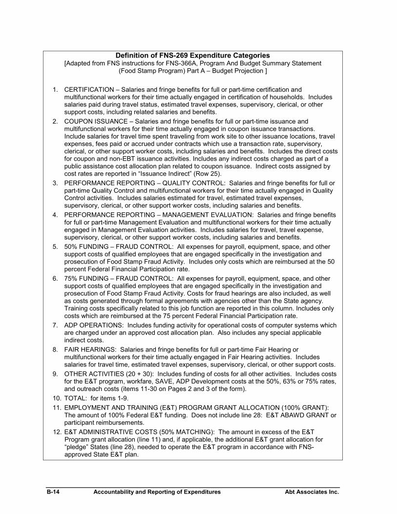
B-14 Accountability and Reporting of Expenditures Abt Associates Inc.
Definition of FNS-269 Expenditure Categories[Adapted from FNS instructions for FNS-366A, Program And Budget Summary Statement
(Food Stamp Program) Part A – Budget Projection ]
1. CERTIFICATION – Salaries and fringe benefits for full or part-time certification andmultifunctional workers for their time actually engaged in certification of households. Includessalaries paid during travel status, estimated travel expenses, supervisory, clerical, or othersupport costs, including related salaries and benefits.
2. COUPON ISSUANCE – Salaries and fringe benefits for full or part-time issuance andmultifunctional workers for their time actually engaged in coupon issuance transactions.Include salaries for travel time spent traveling from work site to other issuance locations, travelexpenses, fees paid or accrued under contracts which use a transaction rate, supervisory,clerical, or other support worker costs, including salaries and benefits. Includes the direct costsfor coupon and non-EBT issuance activities. Includes any indirect costs charged as part of apublic assistance cost allocation plan related to coupon issuance. Indirect costs assigned bycost rates are reported in “Issuance Indirect” (Row 25).
3. PERFORMANCE REPORTING – QUALITY CONTROL: Salaries and fringe benefits for full orpart-time Quality Control and multifunctional workers for their time actually engaged in QualityControl activities. Includes salaries estimated for travel, estimated travel expenses,supervisory, clerical, or other support worker costs, including salaries and benefits.
4. PERFORMANCE REPORTING – MANAGEMENT EVALUATION: Salaries and fringe benefitsfor full or part-time Management Evaluation and multifunctional workers for their time actuallyengaged in Management Evaluation activities. Includes salaries for travel, travel expense,supervisory, clerical, or other support worker costs, including salaries and benefits.
5. 50% FUNDING – FRAUD CONTROL: All expenses for payroll, equipment, space, and othersupport costs of qualified employees that are engaged specifically in the investigation andprosecution of Food Stamp Fraud Activity. Includes only costs which are reimbursed at the 50percent Federal Financial Participation rate.
6. 75% FUNDING – FRAUD CONTROL: All expenses for payroll, equipment, space, and othersupport costs of qualified employees that are engaged specifically in the investigation andprosecution of Food Stamp Fraud Activity. Costs for fraud hearings are also included, as wellas costs generated through formal agreements with agencies other than the State agency.Training costs specifically related to this job function are reported in this column. Includes onlycosts which are reimbursed at the 75 percent Federal Financial Participation rate.
7. ADP OPERATIONS: Includes funding activity for operational costs of computer systems whichare charged under an approved cost allocation plan. Also includes any special applicableindirect costs.
8. FAIR HEARINGS: Salaries and fringe benefits for full or part-time Fair Hearing ormultifunctional workers for their time actually engaged in Fair Hearing activities. Includessalaries for travel time, estimated travel expenses, supervisory, clerical, or other support costs.
9. OTHER ACTIVITIES (20 + 30): Includes funding of costs for all other activities. Includes costsfor the E&T program, workfare, SAVE, ADP Development costs at the 50%, 63% or 75% rates,and outreach costs (items 11-30 on Pages 2 and 3 of the form).
10. TOTAL: for items 1-9.11. EMPLOYMENT AND TRAINING (E&T) PROGRAM GRANT ALLOCATION (100% GRANT):
The amount of 100% Federal E&T funding. Does not include line 28: E&T ABAWD GRANT orparticipant reimbursements.
12. E&T ADMINISTRATIVE COSTS (50% MATCHING): The amount in excess of the E&TProgram grant allocation (line 11) and, if applicable, the additional E&T grant allocation for“pledge” States (line 28), needed to operate the E&T program in accordance with FNS-approved State E&T plan.
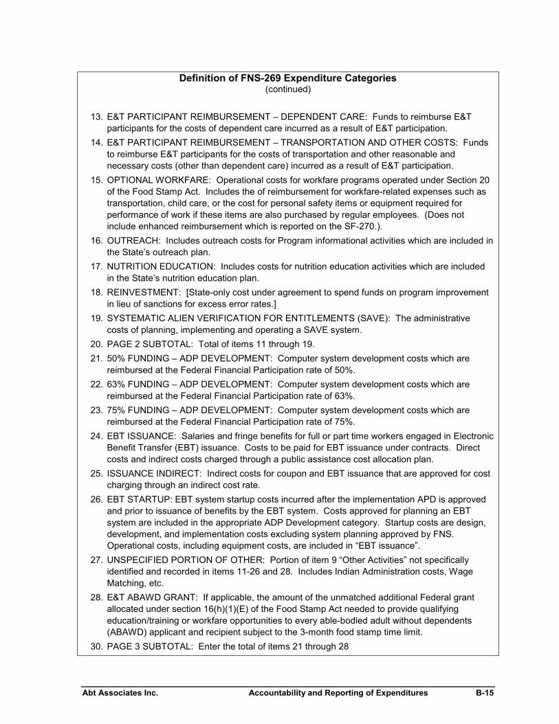
Abt Associates Inc. Accountability and Reporting of Expenditures B-15
Definition of FNS-269 Expenditure Categories(continued)
13. E&T PARTICIPANT REIMBURSEMENT – DEPENDENT CARE: Funds to reimburse E&Tparticipants for the costs of dependent care incurred as a result of E&T participation.
14. E&T PARTICIPANT REIMBURSEMENT – TRANSPORTATION AND OTHER COSTS: Fundsto reimburse E&T participants for the costs of transportation and other reasonable andnecessary costs (other than dependent care) incurred as a result of E&T participation.
15. OPTIONAL WORKFARE: Operational costs for workfare programs operated under Section 20of the Food Stamp Act. Includes the of reimbursement for workfare-related expenses such astransportation, child care, or the cost for personal safety items or equipment required forperformance of work if these items are also purchased by regular employees. (Does notinclude enhanced reimbursement which is reported on the SF-270.).
16. OUTREACH: Includes outreach costs for Program informational activities which are included inthe State’s outreach plan.
17. NUTRITION EDUCATION: Includes costs for nutrition education activities which are includedin the State’s nutrition education plan.
18. REINVESTMENT: [State-only cost under agreement to spend funds on program improvementin lieu of sanctions for excess error rates.]
19. SYSTEMATIC ALIEN VERIFICATION FOR ENTITLEMENTS (SAVE): The administrativecosts of planning, implementing and operating a SAVE system.
20. PAGE 2 SUBTOTAL: Total of items 11 through 19.
21. 50% FUNDING – ADP DEVELOPMENT: Computer system development costs which arereimbursed at the Federal Financial Participation rate of 50%.
22. 63% FUNDING – ADP DEVELOPMENT: Computer system development costs which arereimbursed at the Federal Financial Participation rate of 63%.
23. 75% FUNDING – ADP DEVELOPMENT: Computer system development costs which arereimbursed at the Federal Financial Participation rate of 75%.
24. EBT ISSUANCE: Salaries and fringe benefits for full or part time workers engaged in ElectronicBenefit Transfer (EBT) issuance. Costs to be paid for EBT issuance under contracts. Directcosts and indirect costs charged through a public assistance cost allocation plan.
25. ISSUANCE INDIRECT: Indirect costs for coupon and EBT issuance that are approved for costcharging through an indirect cost rate.
26. EBT STARTUP: EBT system startup costs incurred after the implementation APD is approvedand prior to issuance of benefits by the EBT system. Costs approved for planning an EBTsystem are included in the appropriate ADP Development category. Startup costs are design,development, and implementation costs excluding system planning approved by FNS.Operational costs, including equipment costs, are included in “EBT issuance”.
27. UNSPECIFIED PORTION OF OTHER: Portion of item 9 “Other Activities” not specificallyidentified and recorded in items 11-26 and 28. Includes Indian Administration costs, WageMatching, etc.
28. E&T ABAWD GRANT: If applicable, the amount of the unmatched additional Federal grantallocated under section 16(h)(1)(E) of the Food Stamp Act needed to provide qualifyingeducation/training or workfare opportunities to every able-bodied adult without dependents(ABAWD) applicant and recipient subject to the 3-month food stamp time limit.
30. PAGE 3 SUBTOTAL: Enter the total of items 21 through 28

B-16 Accountability and Reporting of Expenditures Abt Associates Inc.

Appendix CTopic Guides for Federal Agency Interviews

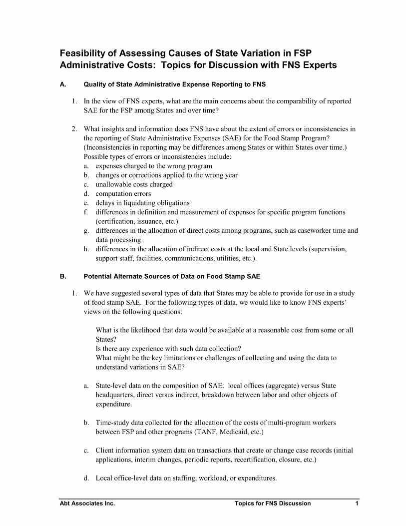
Abt Associates Inc. Topics for FNS Discussion 1
Feasibility of Assessing Causes of State Variation in FSPAdministrative Costs: Topics for Discussion with FNS Experts
A. Quality of State Administrative Expense Reporting to FNS
1. In the view of FNS experts, what are the main concerns about the comparability of reportedSAE for the FSP among States and over time?
2. What insights and information does FNS have about the extent of errors or inconsistencies inthe reporting of State Administrative Expenses (SAE) for the Food Stamp Program?(Inconsistencies in reporting may be differences among States or within States over time.)Possible types of errors or inconsistencies include:a. expenses charged to the wrong programb. changes or corrections applied to the wrong yearc. unallowable costs chargedd. computation errorse. delays in liquidating obligationsf. differences in definition and measurement of expenses for specific program functions
(certification, issuance, etc.)g. differences in the allocation of direct costs among programs, such as caseworker time and
data processingh. differences in the allocation of indirect costs at the local and State levels (supervision,
support staff, facilities, communications, utilities, etc.).
B. Potential Alternate Sources of Data on Food Stamp SAE
1. We have suggested several types of data that States may be able to provide for use in a studyof food stamp SAE. For the following types of data, we would like to know FNS experts’views on the following questions:
What is the likelihood that data would be available at a reasonable cost from some or allStates?Is there any experience with such data collection?What might be the key limitations or challenges of collecting and using the data tounderstand variations in SAE?
a. State-level data on the composition of SAE: local offices (aggregate) versus Stateheadquarters, direct versus indirect, breakdown between labor and other objects ofexpenditure.
b. Time-study data collected for the allocation of the costs of multi-program workersbetween FSP and other programs (TANF, Medicaid, etc.)
c. Client information system data on transactions that create or change case records (initialapplications, interim changes, periodic reports, recertification, closure, etc.)
d. Local office-level data on staffing, workload, or expenditures.
Abt Associates Inc. Topics for FNS Discussion 2
C. FSP Administrative Budgets for States
1. What information do States submit on their administrative budgets the FSP? What revisionsto this information occur, if any?
2. What information does FNS retain on State FSP administrative budgets? Can an electronicfile be produced?
3. What might be the challenges of analyzing the variation in State FSP administrative budgetsand their relationship to actual SAE?
D. Possible Explanations of Variation in Food Stamp SAE Between States
1. What are the most plausible explanations for why food stamp SAE varies so much betweenStates?
2. What information is missing that might help select among these explanations?
Abt Associates Inc. Topics for HHS Discussion 1
Feasibility of Explaining Interstate Differences in Food StampProgram Administrative Costs: Topics for Discussion withDepartment of Health and Human Services Experts
A. Quality of State Administrative Expense Reporting to HHS
1. What are the main factors affecting the comparability of reported administrative expendituresamong States and over time?
2. What insights and information does HHS have about the extent of errors or inconsistencies inthe reporting of State administrative expenditures for the TANF program and other publicassistance programs administered by the FS/TANF agency? (Inconsistencies in reporting maybe differences among States or within States over time.) Possible types of errors orinconsistencies include:a. unallowable costsb. differences in the allocation of shared direct costs among programs, such as caseworker
time and data processingc. differences in the allocation of indirect costs at the local and State levels (supervision,
support staff, facilities, communications, utilities, etc.).
B. Potential Alternate Sources of Data on SAE
1. We have suggested the following types of data that States may be able to provide for use in astudy of food stamp SAE.
a. Time-study data collected for the allocation of the costs of multi-program workersbetween FSP and other programs (TANF, Medicaid, etc.)
b. Client information system data on transactions that create or change case records (initialapplications, interim changes, periodic reports, recertification, closure, etc.)
c. Local office-level data on staffing, pay rates, workload, or expenditures.
d. Local office characteristics (location, programs with joint eligibility determination, otherlocal options)
For these data, we would like to know HHS experts’ views on the following questions: Is there documentation of these data available from HHS? Do States submit any of these data to HHS? What is the likelihood that data would be available at a reasonable cost from some or
all States? What is known about the quality of these data and the steps taken by States to assure
quality? Is there any experience with collecting these data for studies of administrative costs? What might be the key limitations or challenges of collecting and using the data to
understand variations in SAE?
Abt Associates Inc. Topics for HHS Discussion 2
C. State Administrative Budgets for Public Assistance Programs
1. What information, if any, do States submit to HHS on their administrative budgets for publicassistance programs? What revisions to this information occur, if any?
2. What information does HHS retain on State administrative budgets for public assistanceprograms? Can an electronic file be produced?
3. What might be the challenges of analyzing the variation in State administrative budgets forpublic assistance programs and their relationship to actual expenditures?
D. Possible Explanations of Variation in Administrative Spending Between States
1. From your experience, what are the most plausible explanations for why administrativespending for public assistance programs varies between States?
2. What information might help select among these explanations?
Abt Associates Inc. Topics for Regional Office Discussions 1
Feasibility of Explaining Interstate Differences in Food StampProgram Administrative Costs:Topics for Regional Office Discussions
A. Quality of State Administrative Expense Reporting to FNS
1. What kinds or errors or inconsistencies occur in the reporting of State AdministrativeExpenses (SAE) for the Food Stamp Program? (Inconsistencies in reporting may bedifferences among States or within a State over time.) Possible types of errors orinconsistencies include:
a. expenses charged to the wrong program
b. differences in the allocation of direct costs among programs, such as caseworker time anddata processing
c. differences in the allocation of indirect costs at the local and State levels (supervision,support staff, facilities, communications, utilities, etc.).
B. Questions about States Selected for Interviews
1. The purpose of the State interviews in this study is to collect information on the feasibility ofpossible studies of State administrative expenses. Are there reasons that the State selected inthis region would not be a good candidate for these interviews?
a. Probes: new FSP director, audit issues with SAE, budget disputes with FNS,problems with ADP operations or development
2. Is this State or some other State in this region likely to have particularly good analyses or datato support analyses of any of the following types of information?
a. Local office FSP staffing and staff/client ratios (planned or actual)
b. Average pay rates, years of service, and qualifications for local office FSP workers
c. Average time to complete major FSP certification tasks (screening, initialcertification, periodic reports, other interim actions, recertification, closings)—overall, by case type
d. Frequency of principal FSP certification tasks (overall, by case type)
e. Composition of FSP SAE:
i. local offices (aggregate) versus State FSP agency vs. other State agencies(shared services)
ii. breakdown between direct labor, other direct costs, and indirect costs
iii. breakdown of indirect costs by cost pool
f. Use of specialized vs. generalist workers, screeners, etc.
g. FSP expenses for individual local offices or counties/cities
2 Topics for Regional Office Discussions Abt Associates Inc.
h. Error rates, timeliness, or other performance indicators for individual local offices orcounties/cities
3. Who would be the best contacts in the selected State to discuss the availability and quality ofthese data?
C. Possible Explanations of Variation in Food Stamp SAE Between States
1. From your experience, what are the most plausible explanations for why food stamp SAEvaries so much between States?
2. What information might help select among these explanations?

Appendix DState Interview Topic Guide

Abt Associates Inc. Topics for State Agencies 1
Feasibility of Explaining Interstate Differences in Food StampProgram Administrative Costs: Topics for State Interviews
A. Overview of Food Stamp Program (FSP) Administration
Note: The responses to the questions below may vary among local offices. If so, we would like todiscuss this variation.
1. What programs are administered by local Food Stamp offices (other than the FSP) in yourState? (Examples: TANF, Medicaid, Child Support Enforcement, Adoption, Foster Care,Child Welfare)
2. What kinds of local office employees conduct interviews for FSP certification andrecertification? (We are looking for job titles like “eligibility technician”.)
a. Are they FSP-only, multi-program (generic), or a mix of these types?
1.What other programs do multi-program certification workers serve?
b. What other FSP tasks do these employees perform?
1. Other FSP certification (interim changes, reviewing computer match results,etc.)?
2. Other FSP functions (fraud control, employment and training, quality control,fair hearings, outreach, and “other”) ?
3. What other kinds of local office employees do FSP certification-related tasks involving directinteraction with clients? (Example: reception or screening workers.)
a. What FSP certification tasks do these employees perform?
b. What other programs do these employees work on?
c. Do any of these local office employees work on FSP functions other than certification?(Other FSP functions include: fraud control, employment and training, quality control,fair hearings, outreach, and “other”.)
4. What other kinds of local office employees do FSP certification-related tasks that do notinvolve interaction with clients (Examples: filing, data entry, processing change reports)
a. What FSP certification tasks do these employees perform?
b. What other programs do these employees work on?
c. Do any of these local office employees work on FSP functions other than certification?(Other FSP functions include: fraud control, employment and training, quality control,fair hearings, outreach, and “other”.)
5. What other kinds of local office employees work on FSP functions other than certification,such as fraud control, employment and training, quality control, fair hearings, outreach, and“other”?
a. What are the other FSP functions done by these local office employees?
b. For each of these functions:
1. What kinds of employees perform the function?
2 Topics for State Agencies Abt Associates Inc.
2. What other programs do these employees work on?
6. Are any FSP certification tasks handled in regional or central offices of the State agency(such as call centers or change reporting centers)? If so,
a. What client interactions are handled at these locations?
b. What other (“back office”) tasks are handled at these locations?
c. Do the workers perform certification tasks for other programs?
d. Do the workers perform non-certification tasks for the FSP? What are these other FSPtasks?
e. Do the workers perform non-certification tasks for other programs? What are the otherprograms?
7. What FSP functions are contracted out, either to other State agencies or to privateorganizations (community-based organizations, other non-profit organizations, or for-profitcompanies)?
a. What client interactions are handled through these contracts or cooperative agreements?
b. What other (“back office”) FSP tasks are through these contracts or cooperativeagreements?
c. Are similar tasks for other programs handled through these contracts or cooperativeagreements? What are the other programs?
8. What programs share data processing resources with the FSP, such as servers or mainframecomputers, operations and programming staff, and telecommunications networks?
B. Time Studies of Local Office Worker Costs for the Food Stamp Program
1. Does your State conduct a random-moment time study to measure and allocate the costs oflocal FSP certification workers? If so:
a. How often are data collected?
b. About how many local FSP certification workers are in the pool of workers that maybe included in the time study?
c. Are other local FSP workers included, such as supervisors or clerical support? If so,what types?
d. Other than worker salaries, what types of costs are allocated with the time study(such as payroll taxes, fringe benefits, and training)?
e. Approximately how many observations are collected each quarter?
f. What is the average quarterly number of observations per county (or similargeographic unit of local FSP administration, such as district)?
g. What training do workers receive on how to complete the study? May we see a copyof the materials?
2. Does the time study collect data on the type of FSP activity performed?
a. What activities are identified (such as initial certification, periodic or changereporting, recertification, case closing etc.)?
Abt Associates Inc. Topics for State Agencies 3
b. May we see a summary report on the number of observations of each type of activityfor a quarter or longer period?
3. What data are collected on the characteristics of the FSP clients who are served by theactivities measured in the time study? Which of the following data are collected forindividual activities?
a. Whether the household was applying for or approved for public assistance
b. Whether the household was applying for or approved for Medicaid
c. Case number or recipient identifier
d. Other case/recipient characteristics
e. Worker identifier usable for linkage to database of workers (for example, so that timefor an individual activity can be linked to the pay rate or classification of the worker)
4. What data on individual time study observations could be provided for a study ofcertification costs?
a. Are the data from individual observations kept in electronic form?
b. How long are the data on individual observations and summary data retained inelectronic form?
c. Is the database format compatible with off-the-shelf software?
d. What documentation of the data is available? May we see a copy?
e. If data are stored off-line, what is required to access the data?
f. Are there any legal or policy reasons that might prevent a USDA contractor fromusing the data for research?
5. What method(s) are used to measure and allocate the costs of local FSP workers who are notincluded in a time study? (These may be clerical or other support staff, or supervisors.Possible methods might include: counts of activities, time standards, timesheets, caseloaddata, and percentages of hours or full-time equivalents measured in a time study.)For each method, questions a-g will be discussed.
a. What types of local FSP workers are included (caseworkers, clerical support,supervisors, etc.)?
b. What data are collected, by whom, and how often?
c. Other than worker salaries, what types of costs are allocated with the method (such aspayroll taxes, fringe benefits, and training)?
d. How many observations are collected quarterly, statewide and in the averagecounty/district? Do these represent a sample or all activities?
e. Are data collected on the type of FSP activity performed?
1. What activities are identified (such as initial certification, periodic or changereporting, recertification, case closing etc.)?
2. May we see a summary report on the number of observations of each type ofactivity for a quarter or longer period?
4 Topics for State Agencies Abt Associates Inc.
f. What data on individual workers’ time could be provided for a study of certificationcosts? (Refer to B4 for follow-up questions)
6. What data on local office FSP staffing and time use could be provided for a study ofcertification costs? In particular, what existing sources for the following data could be tapped,either as statewide summaries or for individual offices? For the available data, what formare they in, how long are they retained, and are there any barriers to access for research?
a. Local office FSP staffing and staff/client ratios (planned or actual)
b. Average pay rates, years of service, and qualifications for local office FSP workers
c. Average time to complete major FSP certification tasks (screening, initialcertification, periodic reports, other interim actions, recertification, closings)—overall, by case type
d. Frequency of major FSP certification tasks (overall, by case type)
e. Other productivity measures, such as number of actions of specified types per workerper day
7. In the past 10 years, has your State made any changes to the processes for measuring andreporting of the costs of local FSP workers? If so, please describe.
8. What cautions would you suggest regarding the feasibility of using data on local FSP workertime and costs for comparing expenditures across States?
C. Measuring and Allocating Other FSP Costs
1. Other than local office workers, what are the largest cost centers or pools for FSPadministration? (Examples of cost centers include data processing centers and oversight oflocal operations.) For each of these cost centers:
a. What kinds of FSP administrative work does the cost center produce?
b. What types of cost objects are included (salaries, employee benefits, supplies,purchased services, equipment depreciation/usage, facilities rent/usage, utilities,etc.)?
c. How is the share of the cost center for the FSP determined?
d. What are the challenges or problems of measuring and allocating the expenses in thiscost center?
2. In the past 10 years, has your State made any changes to the processes for measuring andreporting of these cost centers costs of local FSP workers? If so, please describe.
3. What cautions would you suggest regarding the feasibility of using data on these cost centerfor comparing expenditures across States?
D. Options for Analyzing Certification-Related Costs
1. Has your agency analyzed differences in FSP certification costs, either among local offices orover time?
a. What data sources were used?
b. What were the findings?
Abt Associates Inc. Topics for State Agencies 5
c. Is a report available? May we see a copy?
2. In your State, what are the potential sources of data from accounting systems for analyzingvariations in the direct and indirect costs of FSP certification? Possible approaches include:
a. Breakdown of FSP certification costs between front-line workers, other local officestaff, other local office costs, and allocated State-level costs
b. Breakdown of FSP certification costs by local office, city, or county
c. Breakdown of FSP “other” costs to determine how much is indirect cost ofcertification
d. What resources and arrangements would be needed to collect these data? What wouldbe the potential problems in collecting and analyzing the data?
3. Does your State have data on variations among local offices in options for organizing staffand client flow, such as use of specialized vs. generalist workers, screeners, etc?
a. What data are available?
b. In what form do the data exist?
c. For what period are the data available?
d. Are there any legal or policy reasons that might prevent a USDA contractor fromusing the data for research?
4. Does your agency have error rates, timeliness, or other FSP performance indicators forindividual local offices or counties/cities?
a. What indicators are collected?
b. How are they used?
c. In what form do the data exist?
d. For what period are the data available?
e. Are there any legal or policy reasons that might prevent a USDA contractor fromusing the data for research?
E. Relationship of Food Stamp Administrative Expenses to Budgets
1. How is the budget set for for local office FSP administration?
a. Is there a specific item or set of items for local FSP administration? If not, whatbudget item includes local FSP administration (such as “income maintenanceadministration” or “local social services”)?
b. What are the roles of the State legislature, your department, and other State officialsin determining the budget item(s) for local FSP administration?
c. What is the time period covered by these budget items (fiscal year, biennium, etc.)?
d. What factors are considered in setting the budget for these items? (Possible factorsinclude caseload, policies, level of automation, and State finances.)
i. Are standards for FSP caseloads or performance used in setting the budget?What are they? How are they set?
6 Topics for State Agencies Abt Associates Inc.
ii. Does the State establish a targeted level of service to FSP clients as part ofthe budget process (tied to funding)?
e. Does the budget change during the fiscal year? Under what circumstances?
f. How is the budget allocated among local offices?
2. How do State and local administrators manage spending against the budget for local officeFSP administration?
a. What happens when the FSP caseload rises?
b. What happens when the FSP caseload falls?
c. What happens when TANF or Medicaid caseloads change?
3. What data on budgets for/including local FSP administration could be provided for a study ofcertification costs?
a. Would the statewide budget that includes local FSP administration be available?
b. Would this budget information be available for areas within the State, such ascounties?
c. What data are available on the assumptions for these budgeted amounts?
d. What form are the data in?
e. How long are they retained?
f. Are there any legal or policy reasons that might prevent a USDA contractor fromusing the data for research?
F. Possible Explanations of Variation in Food Stamp SAE Between States
1. From your experience, what are the most plausible explanations for why food stampcertification costs per case vary between States?
2. What are the factors that affect your State’s automated data processing (ADP) costs per FSPhousehold?
a. How are ADP operating costs affected by system features? What are the key featuresthat affect costs? (These features may include: integration with systems for TANFand/or Medicaid eligibility, support for on-line interviewing, rules-based prompts anderror-checking, on-line access to external data systems (for matching), and datawarehousing and reporting capabilities.)
b. How has the cost of operating your State’s ADP system for the FSP changed since itwas implemented?
c. Does your department use its own data center to host the ADP system for the FSP, ordoes it use a shared facility?
i. Is the data center operated by State employees, a contractor, or a combinationof the two?
ii. When the current data center model was chosen, was there a cost comparisonbetween alternatives? What were the key factors in this decision?
d. What other factors have important impacts on ADP operating costs?
Abt Associates Inc. Topics for State Agencies 7
3. Has your agency analyzed the relationship between ADP costs and local worker costs? If so,
a. What data sources were used?
b. What were the findings?
c. Is a report available for our use?
4. From your knowledge, in what ways is your State’s ADP cost structure similar to anddifferent from most States?
5. What other factors contribute to the variation in total FSP administrative expenses per caseamong States?

8 Topics for State Agencies Abt Associates Inc.
Abt Associates Inc. References R-1
References
American Public Human Services Association (APHSA), 2006. Successful Food Stamp Innovations.www.aphsa.org, accessed October 27, 2007.
Bartlett, S., F. Glantz, and C. Logan, 2008. School Lunch and Breakfast Cost Study-II Final Report.Food and Nutrition Service, USDA, Alexandria, VA CN-08-MCII.
Bartlettt, S., N. Burstein, and W. Hamilton, 2004. Food Stamp Program Access Study: Final Report.Abt Associates Inc. for Economic Research Service, USDA, E-FAN No. (03013-3),http://www.ers.usda.gov/Publications/EFAN03013/EFAN03013-3/.
Bureau of Economic Analysis, 2008. State Annual Personal Income.http://www.bea.gov/regional/spi/, accessed January 7, 2008.
Bureau of Labor Statistics (BLS), 2008a. Occupational Employment Statistics.http://www.bls.gov/oes/home.htm accessed January 7, 2008.
BLS, 2008b. Quarterly Census of Employment and Wages. http://www.bls.gov/cew/home.htm.
BLS, 2008c. National Compensation Survey. http://www.bls.gov/ncs/.
BLS, 2008d. Consumer Price Indexes. http://www.bls.gov/cpi/home.htm, accessed January 7, 2008.
BLS, 2008e. BLS Data on Unions. http://www.bls.gov/bls/blsuniondata.htm.
BLS, 2008f. Local Area Unemployment Statistics. http://www.bls.gov/lau/home.htm
Burstein, N.R., Hamilton, W.L. and Siegel, S.Y., 2008. Understanding the Determinants of FoodStamp Program Participation: Literature Survey. Abt Associates Inc. for Food and NutritionService, USDA, Alexandria VA (draft).
Carmody, K. and Dean. S., 1998. New Federal Food Stamp Restoration for Legal Immigrants:Implications and Implementation Issues. Center on Budget and Policy Priorities, Washington,D.C.
Census Bureau, 2008a. Federal, State, and Local Governments, Public Employment and Payroll Datahttp://www.census.gov/govs/www/apes.html
Census Bureau, 2008b. American Fact Finder. http://factfinder.census.gov.
Census Bureau, 2008c. American Housing Survey Overview.http://www.census.gov/hhes/www/housing/ahs/overview.html
Census Bureau, 2008d. Federal, State, and Local Governments, State and Local GovernmentFinances. http://www.census.gov/govs/www/estimate.html
Census Bureau, 2008e. American Community Survey. http://www.census.gov/acs/www/index.html.
Centers for Medicare and Medicaid Services (CMS), 2008. Medicaid Program Technical Summary.http://www.cms.hhs.gov/MedicaidGenInfo/03_TechnicalSummary.asp.
Cody, S., L. Castner, J. Mabli, and J. Sykes, 2007. Dynamics of Food Stamp Program Participation,2001-2003. Food and Nutrition Service, USDA, Alexandria, VA.
Council for Community Economic Research (C2ER), 2008. ACCRA Cost of Living Index.http://www.coli.org/Method.asp accessed January 7, 2008.

R-2 References Abt Associates Inc.
Department of Defense (DD), 1995. Department of Defense Financial Management Regulation,Volume 4, Chapter 20, “Job Order Cost Accounting”.http://www.defenselink.mil/comptroller/fmr/04/04_20.pdf.
Finegold, K., W. Margrabe, and C. Ratcliffe, 2008. Food Stamp Program Rules DatabaseDocumentation. Prepared by The Urban Institute for the U.S. Department of Agriculture,Economic Research Service, Food Assistance and Nutrition Research Program, Washington,D.C.
FNS, 2006a. Calculating the Food Stamp Program Access Index: A Step-By-Step Guide.http://www.fns.usda.gov/oane/menu/Published/FSP/FILES/Other/PaI2005.pdf accessed1/2/2008.
FNS, 2006b. State Options Report, Sixth Edition. http://www.fns.usda.gov/fsp/rules/Memo/Support/State_Options/sixth/default.htm, accessed January 7, 2008.
FNS, 2007a. Food Stamp Program Participation and Costs (Data as of October 26, 2007).http://www.fns.usda.gov/pd/fssummar.htm, accessed on November 2, 2007.
FNS, 2007b. Request for Proposal (FNS-07-TMN-02) for Proposed Task Order to be issued under theGSA Multiple Award MOBIS Schedule, Statement of Work.
FNS, 2008a. Food and Nutrition Service National Data Bank. Statistics extracted July 2008.FNS,2008b. Electronic Benefits Transfer (EBT) Status Report.http://www.fns.usda.gov/fsp/ebt/ebt_status_report.htm.
FNS, 2008c. Waivers of Rules. http://www.fns.usda.gov/fsp/rules/Waivers/default.htm.
Gatzlaff, D. and C. Holmes, 2007. “Estimating Transaction-Based Price Indices for LocalCommercial Real Estate: An Examination of Methodologies using Property Tax Data.” PaperFor Presentation at the Real Estate Research Institute’s 2007 Annual Conference, Chicago,Illinois, April, 2007. http://www.reri.org/research/article_pdf/wp135.pdf
Goolsby, L., 2004. W-Memo: Food Stamp Administrative Match Reductions. Washington, D.C.:American Public Human Services Association.
Government Accountability Office (GAO), 1999. Food Stamp Program: States Face ReducedFederal Reimbursements for Administrative Costs. Washington, D.C.
GAO, 2000. Food Assistance: Activities and Use of Nonprogram Resources at Six WIC Agencies.Washington, D.C.
GAO, 2003. Food Stamp Employment and Training Program: Better Data Needed to UnderstandWho Is Served and What the Program Achieves. GAO-03-388.
GAO, 2006. Demonstration Projects Could Identify Ways to Simplify Policies and FacilitateTechnology Enhancements to Reduce Administrative Costs. GAO-06-942.
GAO, 2007. Food Stamp Program: Use of Alternative Methods to Apply for and Maintain BenefitsCould Be Enhanced by Additional Evaluation and Information on Promising Practices. GAO-07-573.
Hamilton, W.L., Burstein, N.R., Hart, M.M., Bartlett, S.H., Sullivan, M.B. and Texeira, R.A., 1989.Factors Affecting Food Stamp Certification Cost, Volumes I and II. Alexandria, VA: Food andNutrition Service, USDA.
Abt Associates Inc. References R-3
Health and Human Services (HHS), Department of, 1997. Cost Principles and Procedures forEstablishing Cost Allocation Plans and Indirect Cost Rates for Agreements with the FederalGovernment: A Guide for State, Local and Indian Tribal Governments.
Health and Human Services (HHS), Department of, 2002. Review Guide for Public Assistance CostAllocation Plans. Program Support Center, Division of Cost Allocation, October 2002.http://rates.psc.gov/pacapguide1002.pdf.
Health and Human Services HHS, Department of, 2006. Temporary Assistance for Needy Families(TANF) Seventh Annual Report to Congress, Chapter 12.http://www.acf.hhs.gov/programs/ofa/annualreport7/ar7index.htm
Housing and Urban Development (HUD), Department of, 2008. Fair Market Rents for the Section 8Housing Assistance Payments Program.http://www.huduser.org/datasets/fmr/fmrover_071707R2.doc.
Isaacs, J., 2008. The Costs of Benefit Delivery in the Food Stamp Program: Lessons From a Cross-Program Analysis. Prepared by the Brookings Institution for the Economic Research Service,USDA, Washington D.C.
Kabbani, N.S., and P.E. Wilde, 2003. Short Certification Periods in the U.S. Food Stamp Program.Journal of Human Resources 38, Supplement 2003.
Kirlin, J., N. Cole, and C. Logan, 2003. Assessment of WIC Cost-Containment Practices: FinalReport. Economic Research Service, USDA, Washington, D.C. E-FAN 03-004.
Lewin Group and Rockefeller Institute of Government, 2004. Spending on Social Welfare Programsin Rich and Poor States. Prepared for DHHS, ASPE, Washington, D.C.
Logan, C., J. Kirlin, P. Elwood, M. Menne, and M. Walker, 1994. The Evaluation of the ExpandedEBT Demonstration in Maryland, Volume 2: System Impacts on Program Costs and Integrity.Prepared for the Food and Nutrition Service, USDA, Alexandria, VA.
Logan, C., Rhodes, W., and Sabia, J., 2006. Food Stamp Program Costs and Error Rates, 1989-2001.Economic Research Service, U.S. Department of Agriculture, Washington, D.C., CCR-15.
Logan, C., R. Kling, and W. Rhodes, 2008. Food Stamp Program Certification Costs and Errors,1989-2005. Prepared for the Economic Research Service, USDA, Agreement No. 59-5000-6-0078. Final pre-clearance report submitted to FNS on March 28, 2008.
MaCurdy, T. (1981). "An Empirical Model of Labor Supply in a Life Cycle Setting." Journal ofPolitical Economy. 89(6): 1059-1085.
MaCurdy, T. and Marrufo., G., 2006. The MID-SIPP Model: A Simulation Approach for ProjectingImpacts of Changes in the Food Stamp Program. Washington, D.C: Economic ResearchService, USDA, CCR-24.
Meyer, B. D., 1995. "Natural and Quasi-experiments in Economics," Journal of Business &Economic Statistics, American Statistical Association, vol. 13(2), pages 151-61, April.
Nutt-Powell, B. 1988. Synthesis of Case Study Findings in the WIC Program. Food and NutritionService, USDA, Alexandria, VA.
Phoenix MAXIMUS, 2000. Electronic Benefits Transfer Alternatives Analysis. Prepared for Foodand Nutrition Service, USDA. http://www.fns.usda.gov/fsp/ebt/ebt_alt_analy_appendices.htm.
R-4 References Abt Associates Inc.
Ratcliffe, C., McKernan, S.M, and Finegold, K., 2008. The Effect of State Food Stamp and TANFPolicies on Food Stamp Program Participation. Washington, D.C: Economic ResearchService, USDA.
Real Capital Analytics (RCA), 2008. “Methodology/Sources”.http://www.rcanalytics.com/methodologysources.aspx
Rowe, G. and J. Versteeg, 2005. The Welfare Rules Databook: State Policies as of July 2003. TheUrban Institute. http://www.urban.org/url.cfm?ID=411183.
Schwarz, N., B. Knäuper, D. Oyserman, and C. Stich, 2008. “The psychology of asking questions”,in International Handbook of Survey Methodology Edited by Edith D. de Leeuw, Joop J. Hox,and Don A. Dillman. The Psychology Press, New York, NY.http://www.xs4all.nl/~edithl/surveyhandbook/CH2Schwarz.pdf.
Studley, 2008. “Studley—Research&Ideas”. www.studley.com. accessed May 31, 2008.
University of California Data Archive & Technical Assistance (UC Data) (1999). An Inventory ofResearch Uses of Administrative Data in Social Services Programs in the United States, 1998.Berkeley, CA: University of California, Berkeley.
US Department of Agriculture, Office of Inspector General (USDA-OIG), 2000. Food StampProgram Administrative Costs for the State of Ohio. (Report No: 27099-0020-Ch.)http://www.usda.gov/oig/webdocs/27099-0020-Ch.Pdf
USDA-OIG, 2001. Food Stamp Program Administrative Costs State of Washington (PDF) (ReportNo: 27099-16-SF) http://www.usda.gov/oig/webdocs/27099-16-SF.pdf.
USDA-OIG, 2002. Food Stamp Administrative Costs - California (PDF) (Report No: 27099-18-SF)http://www.usda.gov/oig/webdocs/27099-18-SF.pdf
USDA-OIG, 2003. Food Stamp Employment and Training Program - Tennessee (PDF) (Report No:27601-12-AT). http://www.usda.gov/oig/webdocs/27601-12-At.pdf
Ver Ploeg, M., R. A. Moffitt, and C. F. Citro, eds., 2001. Studies of Welfare Populations: DataCollection and Research Issues. Panel on Data and Methods for Measuring the Effects ofChanges in Social Welfare Programs, Committee on National Statistics, National ResearchCouncil.
Wolkwitz and Ewell, 2007. Technical Documentation for the Fiscal Year 2006 FSPQC Database andQC Minimodel. Mathematica Policy Research Inc. for Food and Nutrition Service, USDA,Alexandria VA.
Wolkwitz, K. 2007. Characteristics of Food Stamp Households: Fiscal Year 2006, FSP-07-CHAR,Mathematica Policy Research Inc. for Food and Nutrition Service, USDA, Alexandria, VA.
Yilmaz, Y., Hoo, S., Nagowski, M., Rueben, K. and Tannenwald, R., 2006. Measuring FiscalDisparities across the U.S. States: A Representative Revenue System/RepresentativeExpenditure System Approach Fiscal Year 2002. A joint report by the Tax Policy Center andthe New England Public Policy Center at the Federal Reserve Bank of Boston, OccasionalPaper 74, The Urban Institute.