Embed Size (px)
Citation preview

University of Arkansas, FayettevilleScholarWorks@UARK
Theses and Dissertations
5-2017
Feasibility of Using Oxide ThicknessMeasurements for Predicting Crack Growth Ratesin P91 Steel ComponentsRalph Edward Huneycutt IVUniversity of Arkansas, Fayetteville
Follow this and additional works at: http://scholarworks.uark.edu/etd
Part of the Engineering Mechanics Commons, and the Mechanical Engineering Commons
This Thesis is brought to you for free and open access by ScholarWorks@UARK. It has been accepted for inclusion in Theses and Dissertations by anauthorized administrator of ScholarWorks@UARK. For more information, please contact [email protected], [email protected].
Recommended CitationHuneycutt, Ralph Edward IV, "Feasibility of Using Oxide Thickness Measurements for Predicting Crack Growth Rates in P91 SteelComponents" (2017). Theses and Dissertations. 2028.http://scholarworks.uark.edu/etd/2028
Feasibility of Using Oxide Thickness Measurements for Predicting Crack Growth Rates in P91
Steel Components
A thesis submitted in partial fulfillment
of the requirements for the degree of
Master of Science in Mechanical Engineering
by
Ralph E. Huneycutt IV
University of Arkansas
Bachelor of Science in Mechanical Engineering, 2014
May 2017
University of Arkansas
This thesis is approved for recommendation to the Graduate Council.
Dr. Ashok Saxena
Thesis Director
Dr. Rick J. Couvillion
Committee Member
Dr. Paul C. Millett
Committee Member
Abstract
There are only few methods available for predicting the age of cracks that are found in high
temperature structural components during service; among the promising ones is the oxide
thickness measurement technique. Oxide thickness profiles are taken from crack surfaces of
components and used for predicting the rates of crack propagation. This technique is particularly
suitable for high temperature components fabricated from ferritic steels commonly used in power
plants that run on fossil fuels. To implement this technique, it is necessary to fully understand the
kinetics of high temperature oxidation in these steels. In this study, the oxidation characteristics
of an American Society of Testing and Materials (ASTM) Grade P91 ferritic steel used in high
temperature piping is characterized.
The literature shows that there are four primary mechanisms that influence the oxide thickness
during high temperature exposure. Initially, the oxide thickness increases in a linear fashion with
time and then as steady-state conditions are established, the parabolic relationship takes over.
Multiple types of oxides with different rate characteristics can also form. Oxide degradation can
occur by spallation due to porosity and formation of cracks. Evaporation or volatility can also
occur and result in loss of oxide thickness. These factors must be considered in oxide thickness
analysis to determine crack growth history.
Two sets of laboratory experiments were conducted. The first consisted of measurement of oxide
thicknesses after exposure to high temperature for various periods to determine the oxidation
kinetics. The oxidized samples were subjected to SEM examination and measurements of
physical properties such as density and porosity levels. The second set of experiments consisted

of measuring the oxide layer thickness on the fracture surfaces of creep-fatigue crack growth
samples tested as part of a previous study where the crack growth rates were measured. These
reported measurements are used to compare with the predicted crack growth rates from the
analytical models that are developed as part of this study. The success of the technique is
measured by finding the correlation coefficient, which is within a factor of 2.58.

Acknowledgements
I would like to thank my thesis advisor Dr. Ashok Saxena, Distinguished Professor and Dean
Emeritus, of the Mechanical Engineering Department at the University of Arkansas. He
constantly was able to steer me into the right direction, while not micromanaging me. Without
his insights and support this work would not have been possible.
I would also like to thank Dr. Kee Bong Yoon in the School of Mechanical Engineering at
Chung-Ang University in South Korea. I am grateful for his advisement during our meeting and
support during this project.
Finally, I would like to express my gratitude to my family and especially my wife for providing
me with support and encouragement during my studies, research, and writing of this thesis. This
accomplishment would not have been possible without them. Thank you.
Table of Contents
I. Introduction and Research Objectives .................................................................................... 1
II. Objective ................................................................................................................................... 3
III. Literature Review ................................................................................................................... 5
A. Single Layer Oxidation Kinetics ......................................................................................... 5 A.i) The Parabolic Law ........................................................................................................... 5
A.ii) Dependence of the Parabolic Rate Constant on Temperature and Pressure ................... 7
A.iii) Measurement of kp ...................................................................................................... 10
B. Two Layer Scale Growth Kinetics .................................................................................... 12
C. Other Mechanisms Influencing Oxide Thickness ........................................................... 13
D. Validity of parabolic oxide kinetics .................................................................................. 17
E. Using Oxide Growth Kinetics to Determine Crack Growth Rates ................................ 19
IV. Experimental Setup and Process ......................................................................................... 21
A. Experimental Setup............................................................................................................ 21 A.i) Test Material Chosen for Experiments .......................................................................... 21
A.ii) Sample Design and Creation ........................................................................................ 22
B. Experimental Process ......................................................................................................... 24 B.i) Preparation of Oxidation Samples ................................................................................. 24
B.ii) Measurement of Pre-test Sample Mass ......................................................................... 26
B.iii) Oxidation Experiments ................................................................................................ 27
B.iv) Post-Test Mass Gain Measurements ............................................................................ 30
B.v) Application of Protective Ni Coating ........................................................................... 30
B.vi) Measurement of Oxide Profiles and Thicknesses ........................................................ 33
B.vi)(a) SEM Overview ........................................................................................................ 33
B.vi)(b) Sample Preparation ................................................................................................. 35
B.vi)(c) Procedure During SEM ........................................................................................... 37
B.vi)(d) Procedure for Analyzing SEM Photomicrographs .................................................. 39
V. Data Analysis .......................................................................................................................... 42
A. Determination of Parabolic Constant, kp, for Mass Gain .............................................. 42
B. Oxide Growth Measurements ........................................................................................... 48
C. Finding Crack Growth Rates on C(T) ............................................................................. 61
VI. Conclusions and Future Work ............................................................................................ 73
A. Conclusion........................................................................................................................... 73
B. Future Work ....................................................................................................................... 73
C. Improvements ..................................................................................................................... 73
D. Application .......................................................................................................................... 74
VII. References ............................................................................................................................ 76
VII. Appendix .............................................................................................................................. 78
A. Pretest and Posttest Weight of Oxidation Samples ......................................................... 78
B. Parabolic Rate Constants in terms of mg^2*mm^-4*hr^-1 .......................................... 79
C. Different output results of MATLAB© edge Function .................................................. 80
D. Coefficients of Incremental Polynomial Method on C(T) Samples ............................... 81
List of Tables
Table 1 – Parabolic rate constants in air (mg2mm-4hr-1) [15] ................................................... 18 Table 2 – Chemical composition of test material (in weight %)[17] ............................................ 22 Table 3 – Test Matrix .................................................................................................................... 27 Table 4 – Kp for finding Weight Change/Area ............................................................................ 43 Table 5 – Kp for finding Weight Change/Area from Literature[15] ............................................ 43 Table 6 – Weight Gain Parabolic Constant using First Four Data Points .................................... 45 Table 7 – Weight Gain Parabolic Constant using First Four Data Points .................................... 46 Table 8 – Constants of Arrhenius type Equation for Weight Gain ............................................... 48 Table 9 – KP for oxide thickness .................................................................................................. 49 Table 10 – KP for Oxide Thickness at 650 C using First Two Data Points ................................. 51 Table 11 – Weight Gain Parabolic Constant using First Four Data Points .................................. 52 Table 12 – Constants of Arrhenius type Equation for Oxide Thickness ...................................... 53 Table 13 – Activation Energy Values ........................................................................................... 54 Table 14 – Comparable Activation Energy Values[13] ................................................................ 54 Table 15 – Comparison of Activation Energies ............................................................................ 54 Table 16 – Comparing Activation Energy Values ........................................................................ 55 Table 17 – Coefficients of Qavg Curve Fit ................................................................................... 58 Table 18 – Density Constant, ρs and ρs' using Qavg................................................................... 58 Table 19 - Constant for Eq. 38 from Figure 55 ............................................................................ 59 Table 20 – Density Values Calculated from Eq. 38 and 39 .......................................................... 59 Table 21 - Densities of Probable Oxides of P91 Steel[20] ........................................................... 59 Table 22 – Percent Difference Between Oxide Thickness Kp Values from Table 4 and Eq. 28
using Qavg values for Oxide Thickness from Table 15 ................................................... 60 Table 23 – Percent Difference Between Oxide Thickness Kp Values from Table 4
and Kp Values from Eq. 36, Eq. 28 using Qavg for Weight Gain from
Table 15, and Density Constants ...................................................................................... 60
Table 24 – Values to Calculate Kp at 625 C ................................................................................ 60 Table 25 – Percent Difference Between Kp values from Table 4 and Kp values
using Eq. 28 and Table 23................................................................................................. 61 Table 26 - Curve Fit Values from Figure 61 ................................................................................ 68 Table 27 – Percent Difference between Measured tf and Predicted tf ......................................... 69 Table 28 - Correlation Coefficients From Figure 62 .................................................................... 70 Table 29 – Pretest and Posttest Weight at 600°C ......................................................................... 78 Table 30 – Pretest and Posttest Weight at 625°C ......................................................................... 78 Table 31 – Pretest and Posttest Weight at 650°C ......................................................................... 78 Table 32 – Parabolic Rate Constant (mg^2*mm^-4*hr-1) for 600°C .......................................... 79 Table 33 – Parabolic Rate Constant (mg^2*mm^-4*hr^-1) for 625°C ........................................ 79 Table 34 – Parabolic Rate Constant (mg^2*mm^-4*hr^-1) for 650°C ........................................ 79 Table 35 – Incremental Polynomial Method Results for Seven Points for 3.2-9A ...................... 81 Table 36 – Incremental Polynomial Method Results for Seven Points for 3.2-15A .................... 81 Table 37 – Incremental Polynomial Method Results for Seven Points for 3-1-30 ....................... 82 Table 38 – Crack Growth Rates for 3.2-9A .................................................................................. 82 Table 39 – Crack Growth Rates for 3.2-15A ................................................................................ 83 Table 40 – Crack Growth Rates for 3-1-30 .................................................................................. 83

Table 41 – Crack Growth Rate Values for 3.2-9A ....................................................................... 84 Table 42 – Crack Growth Rate Values for 3.2-15A ..................................................................... 84 Table 43 – Crack Growth Rate Values for 3-1-30 ........................................................................ 85
List of Figures
Figure 1 – Schematic of Pipe in Service with Crack with Oxide Growth on
the Crack Surface ................................................................................................................ 3 Figure 2 – Diffusion-Controlled Oxidation mechanism [11] ......................................................... 5 Figure 3 – Graphical Representation of the dependence of the diffusion coefficient of
Ni on Temperature [11] ...................................................................................................... 9 Figure 4 – Variation of parabolic rate constant with oxygen partial pressure and
temperature for the oxidation of copper [10] .................................................................... 10 Figure 5 – Typical Experimental Arrangement for Measuring Oxidation Kinetics [11] ............. 11 Figure 6 – Schematic View of Two-Layer Scale Growth [13] ..................................................... 13 Figure 7 – 1Cr-0.5Mo steel Oxidized in Laboratory air for 1000h at 5000 C [14] ..................... 13 Figure 8 – Ellingham-Richardson Diagram for Selected Oxides [14].......................................... 14 Figure 9 – Different oxidation kinetics frequently encountered in real metal
and alloys systems [14]. .................................................................................................... 17 Figure 10 – Weight change vs. Time for oxidation of various ferritic alloys at
873 K in air [15] ................................................................................................................ 18 Figure 11 – Weight change vs. Time plots for the same alloys as in Figure 10 at
1073 K in O2 + 50 % H2O [15] ....................................................................................... 18 Figure 12 – Oxide thickness as a function of crack length for thumbnail defect in
C-Mn Steel pipe. [10] ....................................................................................................... 19 Figure 13 – Crack length as a function of time derived from oxide thickness measurements
shown in Figure 12 [10] .................................................................................................... 19 Figure 14 - Picture of the pipe from which the test material for the program was extracted. ...... 22 Figure 15 - Picture of a tested creep-fatigue crack growth specimen used for
machining the oxidation samples. ..................................................................................... 23 Figure 16 – CAD of Oxidation Samples ....................................................................................... 24 Figure 17 - A special sample holder created to ensure uniform polish on all surfaces ................ 25 Figure 18 - Polishing paper taped to the work surface for polishing samples .............................. 26 Figure 19 – Satorius Cubis MSA225S-100-DI used for Measuring Weight Change ................... 27 Figure 20 – Picture of the furnace being used for oxidation tests as part of the
2330 Series Creep/Stress Rupture Testing System ........................................................... 28 Figure 21 – CAD of Dummy Samples .......................................................................................... 29 Figure 22– Results from a trial run of the furnace at 500°C for 100 hours .................................. 29 Figure 23 – Picture of sample holder from 2 views ...................................................................... 30 Figure 24 – Optical contrast created by Ni coating oxidized samples [14] .................................. 31 Figure 25 – E-Beam Evaporator available for Ni coating samples .............................................. 31 Figure 26 – C(T) samples mounted to Si wafer for application of Ni coating ............................. 32 Figure 27 – SEM analysis of the side profile of a fractured C(T) specimen. ............................... 33 Figure 28 – Polished Surface and Fractured Surface [19] ............................................................ 34 Figure 29 – SEM of Fractured Surface with Epoxy Coating ........................................................ 35 Figure 30 – Epoxy Hardening Container with Sample ................................................................. 35 Figure 31 – Sample Polishing with Rotation ................................................................................ 36 Figure 32 - Difference Between SEM Output with and without Filler Material .......................... 37 Figure 33 - C(T) Sample Prepared for SEM with Copper Conductive Tape ............................... 37 Figure 34 – sem sample stage movement control ......................................................................... 38
Figure 35 - MATLAB© Command Window to Pull Images into imtool .................................... 39 Figure 36 - imtool on an EDX SEM Image .................................................................................. 40 Figure 37 - imtool Toolbar ............................................................................................................ 40 Figure 38 - Zoomed in Output of Measure Distance Icon ............................................................ 40 Figure 39 - Output for One Location using MATLAB©’s imtool ............................................... 41 Figure 40 – (Weight Gain/Area) vs Time all Data Points ............................................................ 42 Figure 41 – (Weight Gain/Area)^2 vs Time to Find Kp Values ................................................... 43 Figure 42 – Ln (Kp) versus 1/Temperature ................................................................................... 44 Figure 43 – Divergence from Parabolic Model for Weight Gain at 650 C .................................. 45 Figure 44 – Weight Gain at 650 C using Eq. 25 ........................................................................... 46 Figure 45 – Figure 42 redrawn with updated Kp For 650 C ......................................................... 47 Figure 46 – ln (Kp) for weight gain versus 1/Temperature .......................................................... 48 Figure 47 – Oxide Thickness vs Time .......................................................................................... 49 Figure 48 – (Oxide Thickness)^2 vs Time ................................................................................... 50 Figure 49 – (Oxide Thickness)^2 vs Time without 625 C 1000 hr .............................................. 50 Figure 50 - Divergence from Parabolic Model for Oxide Thickness at 650 C ............................. 51 Figure 51 – Oxide Thickness at 650 using Eq. 25 ........................................................................ 52 Figure 52 – ln(KP) for Oxide Thickness vs Temp^-1 ................................................................... 53 Figure 53 – Weight Gain ln(Kp) using Qavg versus Qwg for 600, 625, and 650 C .................... 57 Figure 54 – Oxide Thickness ln(Kp) using Qavg versus Qwg for 600, 625, and 650 C .............. 57 Figure 55 - Weight Gain/Area vs Oxide Thickness ...................................................................... 58 Figure 56 – R.R. Crack Extension vs Time .................................................................................. 61 Figure 57 – Crack Growth Rates for C(T) Specimens .................................................................. 62 Figure 58 - ideal crack extension versus oxide thickness ............................................................. 63 Figure 59 – Crack Extension vs Oxide Thickness ........................................................................ 65 Figure 60 – Difference Between Raw Data (a) and AVG Data (b) .............................................. 67 Figure 61 – C(T) Samples’ Crack Extension vs Oxide Thickness Curve Fit ............................... 68 Figure 62 – Correlation Between Predicted Crack Growth Rates and Measured ........................ 70 Figure 63 – Measured and Predicted Crack Growth Rates vs Crack Extension ........................... 72 Figure 64 – Idealize Component with Known Crack ................................................................... 74 Figure 65 – Oxide thickness profile with Epoxy Coating ............................................................ 75 Figure 66 – Different Threshold Values for Canny Edge Method with MATLAB© .................. 80
1
I. Introduction and Research Objectives
The ability to operate fossil-fuel-fired power plants reliably and to boost their operating
temperature capability to attain higher energy conversion efficiencies is essential for the future of
the electric power generation industry. Several components of power plants such as reheat
piping, heat recovery steam generator (HRSG) Boilers, turbine casings, steam headers and
turbine rotors are subjected to high temperatures and periodic cyclic loading during their
operation that cause damage in the form of creep cavities and the formation of cracks due to the
phenomena such as creep and creep-fatigue interactions. The operators of such equipment
frequently use plastic replicas to monitor the progression of damage. Accurate models are needed
to assess the level of damage and the remaining life to make run/repair/retire decisions.
In the past twenty years, considerable progress has been made in the ability to predict crack
growth and damage propagation under the conditions of creep and creep-fatigue [1-6]. Due to the
large number of variables and material constants needed in the analysis, the variability in the life
predictions can be as high as a factor of ten [7]. The use of oxide thickness measurements from
the extracted damaged regions of the reheat steam pipes to directly measure crack growth rates
during service to verify predictions from the analytical crack growth models is explored in this
study. The comparisons between theoretical predictions and actual measurements can be to
improve the accuracy of the analytical models [7].
The material chosen for this research is ASTM Grade P91 steel used in steam pipes in advanced
power plants. The test material is taken from an ex-service steam pipe but rejuvenated to recover
the original microstructure. This material has been used as the test material for conducting two
round–robins to verify test standards developed by American Society for Testing and Materials

2
(ASTM) in the areas of creep-fatigue crack formation and crack growth, E-2714-09 and E-2760-
10, respectively [8,9]. Consequently, considerable crack growth data and tested specimen
fracture surfaces were available to support the project objectives.
3
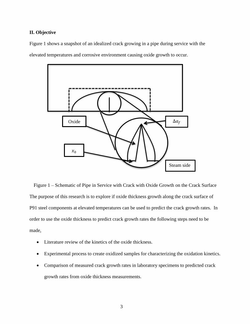
II. Objective
Figure 1 shows a snapshot of an idealized crack growing in a pipe during service with the
elevated temperatures and corrosive environment causing oxide growth to occur.
Figure 1 – Schematic of Pipe in Service with Crack with Oxide Growth on the Crack Surface
The purpose of this research is to explore if oxide thickness growth along the crack surface of
P91 steel components at elevated temperatures can be used to predict the crack growth rates. In
order to use the oxide thickness to predict crack growth rates the following steps need to be
made,
Literature review of the kinetics of the oxide thickness.
Experimental process to create oxidized samples for characterizing the oxidation kinetics.
Comparison of measured crack growth rates in laboratory specimens to predicted crack
growth rates from oxide thickness measurements.
𝑥0
Oxide ∆𝑎𝑓
Steam side

4
The literature review begins with a description of the growth kinetics of a simplified model that
considers only a single layer of oxide.
5
III. Literature Review
A. Single Layer Oxidation Kinetics
A.i) The Parabolic Law
The idea of using the oxide thickness as a parameter of predicting the age of a cracks and
estimating propagation rates was first introduced by L.W. Pinder [10]. In this paper, the kinetics
of oxide growth is used to determine the amount of service time the crack has been in the
component and the rate at which it has been growing. A basic model of oxide growth kinetics
can be derived through the illustration shown in Figure 2 for a diffusion-controlled oxidation
process.
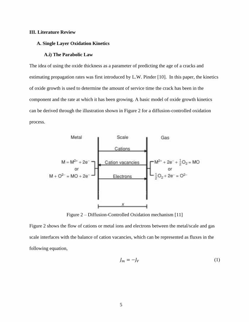
Figure 2 – Diffusion-Controlled Oxidation mechanism [11]
Figure 2 shows the flow of cations or metal ions and electrons between the metal/scale and gas
scale interfaces with the balance of cation vacancies, which can be represented as fluxes in the
following equation,
𝐽𝑚 = −𝐽𝑉 (1)
6
where 𝐽𝑚 is the flux of the metal ions and the electrons and 𝐽𝑣 is the flux of the cation and
electron vacancies. Using Eq. 1, the flux of the metal atoms into the oxide scale can be rewritten
into,
𝐽𝑚 = 𝐷𝑣,𝑚𝑑𝐶𝑣,𝑚
𝑑𝑥 (2)
where 𝐷𝑣,𝑚 is the vacancy diffusion coefficient in the metal and 𝑑𝐶𝑣,𝑚
𝑑𝑥 is the gradient of vacancy
concentration in the x-direction. Next, we assume that the scale is thick enough for the
metal/scale and scale/gas interfaces to be in thermodynamic equilibrium. This assumption
allows the change in concentration in the x-direction to be altered in Eq. 2 into,
𝐽𝑚 = 𝐷𝑣,𝑚𝐶𝑣,𝑚
′′ −𝐶𝑣,𝑚′
𝑥 (3)
where 𝐶𝑣,𝑚′′ is the composition at the scale/gas interface, 𝐶𝑣,𝑚
′ is the composition at the
metal/scale interface, and x is the length (or thickness) of the scale. The next modeling step is to
relate the flux of the metal atoms to the rate of change of the scale thickness using the following
relationship,
𝐽𝑚 =1
𝑉𝑠
𝑑𝑥
𝑑𝑡 (4)
Where 𝑉𝑠 is the molar volume of the scale and 𝑑𝑥
𝑑𝑡 is the rate of change in the oxide thickness over
time. Combining Eq. 3 and 4 leads to the rate of change of the oxide scale thickness in terms of
the vacancy concentration across the oxide scale,
𝑑𝑥
𝑑𝑡= 𝑉𝑠𝐷𝑣,𝑚
𝐶𝑣,𝑚′′ −𝐶𝑣,𝑚
′
𝑥 (5)
Using the assumptions that the system is in steady state and under isothermal conditions, the
following terms can be combined together in a single term known as the parabolic rate constant,
𝑘𝑝,
7
𝑘𝑝 = 𝑉𝑠𝐷𝑣,𝑚(𝐶𝑣,𝑚′′ − 𝐶𝑣,𝑚
′ ) (6)
Using Eq. 5 and 6 the rate of change of the oxide scale thickness is written as,
𝑑𝑥
𝑑𝑡=
𝑘𝑝
𝑥 (7)
Integrating Eq. 7 from t =0 when x =0 to an arbitrary time, t, corresponding to the oxide
thickness, x, yields the following relationship,
∫ 𝑥
𝑥
0
𝑑𝑥 = ∫ 𝑘𝑝
𝑡
0
𝑑𝑥
𝑥2 = 2𝑘𝑝𝑡 (8)
Equation 8 is known as the parabolic rate equation explicitly relating oxide thickness to the time
of exposure to the oxidizing environment. The factor of 2 in Equation 8 is incorporated into the
parabolic rate constant, 𝑘𝑝, during the data analysis but in Birks, Meier, and Pettit[11] and
Young[13] the factor of 2 is kept. Therefore, the oxidation kinetics are represented by the in the
following relationship for isothermal conditions,
𝑥2 = 𝑘𝑝𝑡 (9)
A.ii) Dependence of the Parabolic Rate Constant on Temperature and Pressure
The parabolic rate constant, 𝑘𝑝varies with temperature through its relationship with the self-
diffusion coefficient that is dependent on the kinetics of vacancy diffusion. The self-diffusion
coefficient, D*, in a three-dimensional crystal is [12],
𝐷∗ =𝜆2Γ𝑎
6 (10)
where 𝐷∗ is the self-diffusion coefficient, 𝜆 is the mean atomic spacing, and Γ𝑎 is the atomic
jump frequency. The vacancy diffusion coefficient in a three-dimensional system is,
𝐷𝑣 =𝜆2Γ𝑣
6 (11)

8
where Γ𝑣 is the vacancy jump frequency. The two jump frequencies are related because the
number of atomic jumps equals the number of vacancy jumps; thus,
𝑛𝑣Γ𝑣 = 𝑛𝑎Γ𝑎 (12)
where 𝑛𝑣 is the moles of vacancies and 𝑛𝑎 is the moles of atoms. Since the total moles of the
system, 𝑛, is equal to the moles of vacancies plus the mole of atoms, dividing both sides of the
equation by the total moles of the system modifies Eq. 12 into,
𝑋𝑣Γ𝑣 = 𝑋𝑎Γ𝑎 (13)
where 𝑋𝑣 is the mole fraction of vacancies and 𝑋𝑎 is the atomic mole fraction of atoms. Since
the 𝑋𝑎 ≈ 1, Eq. 13 can be simplified into,
𝑋𝑣Γ𝑣 = Γ𝑎 (14)
The reason Eq.14 is significant is because the self-diffusion coefficient is also equal to,
𝐷∗ = 𝐷0exp (−𝑄
𝑅𝑇) (15)
where 𝐷0 is the pre-exponential coefficient, Q is the activation energy, R is the ideal gas
constant, and T is the temperature, which means the diffusion coefficient is exponentially
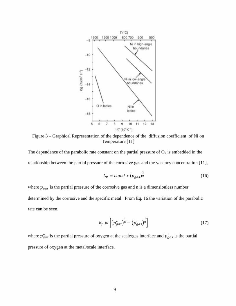
dependent on temperature and therefore also 𝑘𝑝 as seen in Figure 3 for Ni. The diffusion
coefficient is plotted in an Arrhenius type plot for lattice diffusion and also grain boundary
diffusion through low angle and high angle grain boundaries. It also plots the diffusion of oxygen
in Ni.
9
Figure 3 – Graphical Representation of the dependence of the diffusion coefficient of Ni on
Temperature [11]
The dependence of the parabolic rate constant on the partial pressure of O2 is embedded in the
relationship between the partial pressure of the corrosive gas and the vacancy concentration [11],
𝐶𝑣 = 𝑐𝑜𝑛𝑠𝑡 ∗ (𝑝𝑔𝑎𝑠)1
𝑛 (16)
where 𝑝𝑔𝑎𝑠 is the partial pressure of the corrosive gas and n is a dimensionless number
determined by the corrosive and the specific metal. From Eq. 16 the variation of the parabolic
rate can be seen,
𝑘𝑝 ∝ [(𝑝𝑔𝑎𝑠′′ )
1
𝑛 − (𝑝𝑔𝑎𝑠′ )
1
𝑛] (17)
where 𝑝𝑔𝑎𝑠′′ is the partial pressure of oxygen at the scale/gas interface and 𝑝𝑔𝑎𝑠
′ is the partial
pressure of oxygen at the metal/scale interface.
10
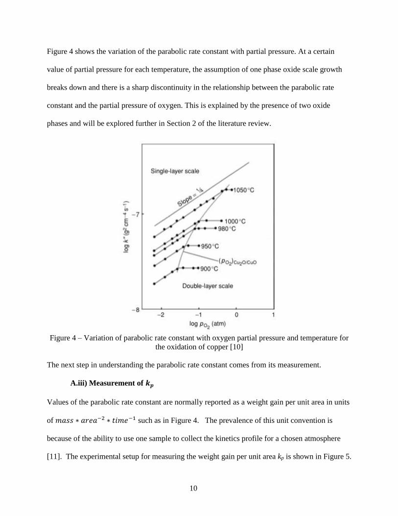
Figure 4 shows the variation of the parabolic rate constant with partial pressure. At a certain
value of partial pressure for each temperature, the assumption of one phase oxide scale growth
breaks down and there is a sharp discontinuity in the relationship between the parabolic rate
constant and the partial pressure of oxygen. This is explained by the presence of two oxide
phases and will be explored further in Section 2 of the literature review.
Figure 4 – Variation of parabolic rate constant with oxygen partial pressure and temperature for
the oxidation of copper [10]
The next step in understanding the parabolic rate constant comes from its measurement.
A.iii) Measurement of 𝒌𝒑
Values of the parabolic rate constant are normally reported as a weight gain per unit area in units
of 𝑚𝑎𝑠𝑠 ∗ 𝑎𝑟𝑒𝑎−2 ∗ 𝑡𝑖𝑚𝑒−1 such as in Figure 4. The prevalence of this unit convention is
because of the ability to use one sample to collect the kinetics profile for a chosen atmosphere
[11]. The experimental setup for measuring the weight gain per unit area kp is shown in Figure 5.
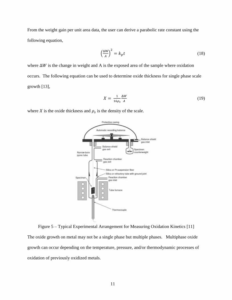
11
From the weight gain per unit area data, the user can derive a parabolic rate constant using the
following equation,
(ΔW
𝐴)
2
= 𝑘𝑝𝑡 (18)
where Δ𝑊 is the change in weight and A is the exposed area of the sample where oxidation
occurs. The following equation can be used to determine oxide thickness for single phase scale
growth [13],
𝑋 = 1
16𝜌𝑠
Δ𝑊
𝐴 (19)
where 𝑋 is the oxide thickness and 𝜌𝑠 is the density of the scale.
Figure 5 – Typical Experimental Arrangement for Measuring Oxidation Kinetics [11]
The oxide growth on metal may not be a single phase but multiple phases. Multiphase oxide
growth can occur depending on the temperature, pressure, and/or thermodynamic processes of
oxidation of previously oxidized metals.
12
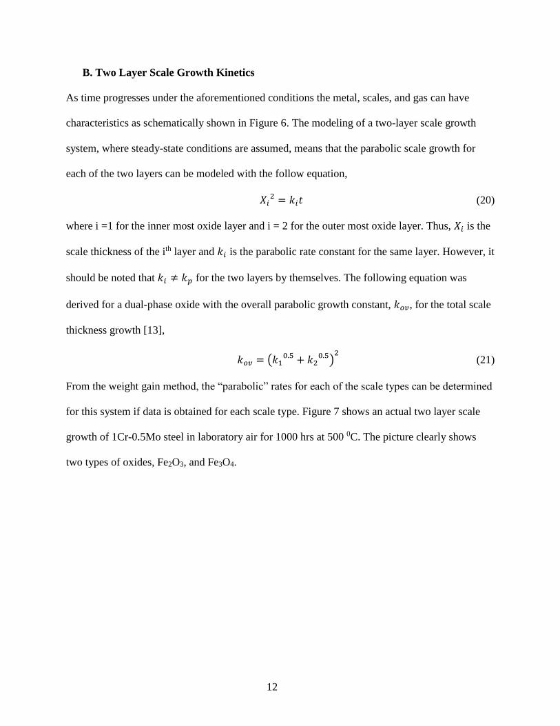
B. Two Layer Scale Growth Kinetics
As time progresses under the aforementioned conditions the metal, scales, and gas can have
characteristics as schematically shown in Figure 6. The modeling of a two-layer scale growth
system, where steady-state conditions are assumed, means that the parabolic scale growth for
each of the two layers can be modeled with the follow equation,
𝑋𝑖2 = 𝑘𝑖𝑡 (20)
where i =1 for the inner most oxide layer and i = 2 for the outer most oxide layer. Thus, 𝑋𝑖 is the
scale thickness of the ith layer and 𝑘𝑖 is the parabolic rate constant for the same layer. However, it
should be noted that 𝑘𝑖 ≠ 𝑘𝑝 for the two layers by themselves. The following equation was
derived for a dual-phase oxide with the overall parabolic growth constant, 𝑘𝑜𝑣, for the total scale
thickness growth [13],
𝑘𝑜𝑣 = (𝑘10.5 + 𝑘2
0.5)2 (21)
From the weight gain method, the “parabolic” rates for each of the scale types can be determined
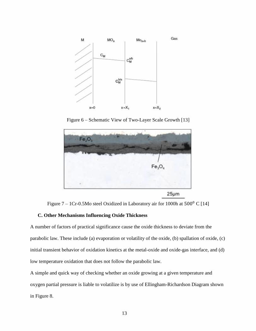
for this system if data is obtained for each scale type. Figure 7 shows an actual two layer scale
growth of 1Cr-0.5Mo steel in laboratory air for 1000 hrs at 500 0C. The picture clearly shows
two types of oxides, Fe2O3, and Fe3O4.
13
Figure 6 – Schematic View of Two-Layer Scale Growth [13]
Figure 7 – 1Cr-0.5Mo steel Oxidized in Laboratory air for 1000h at 5000 C [14]
C. Other Mechanisms Influencing Oxide Thickness
A number of factors of practical significance cause the oxide thickness to deviate from the
parabolic law. These include (a) evaporation or volatility of the oxide, (b) spallation of oxide, (c)
initial transient behavior of oxidation kinetics at the metal-oxide and oxide-gas interface, and (d)
low temperature oxidation that does not follow the parabolic law.
A simple and quick way of checking whether an oxide growing at a given temperature and
oxygen partial pressure is liable to volatilize is by use of Ellingham-Richardson Diagram shown
in Figure 8.
14
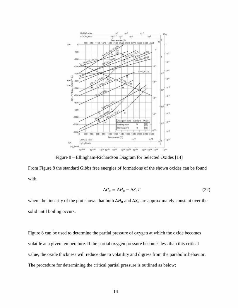
Figure 8 – Ellingham-Richardson Diagram for Selected Oxides [14]
From Figure 8 the standard Gibbs free energies of formations of the shown oxides can be found
with,
∆𝐺0 = ∆𝐻0 − ∆𝑆0𝑇 (22)
where the linearity of the plot shows that both ∆𝐻0 and ∆𝑆0 are approximately constant over the
solid until boiling occurs.
Figure 8 can be used to determine the partial pressure of oxygen at which the oxide becomes
volatile at a given temperature. If the partial oxygen pressure becomes less than this critical
value, the oxide thickness will reduce due to volatility and digress from the parabolic behavior.
The procedure for determining the critical partial pressure is outlined as below:

15
1. Line up a straight edge on the line next to the Gibbs free energy of formation on one of
the points dependent on the critical ratio or partial pressure chosen.
a. If oxygen is the main corrosive agent in the system, place the straight edge on the
point labeled O.
b. If 𝐻2𝑂 is the main corrosive agent in the system, place the straight edge on the
point labeled H.
c. If carbon dioxide is the main corrosive agent system place the straight edge on the
point labeled C.
2. Keeping one part of the straight edge on the point for the type of corrosive and then
rotate the end until the straight edge goes through the intersection of the temperature and
the oxide of interest.
3. Follow the line created by the straight edge and read the partial pressure off of the axis
of the type of corrosive of interest.
The partial pressure value that is found via this method is known as the equilibrium partial
pressure. If the partial pressure of the corrosive is below the equilibrium partial pressure, then
the oxide will become volatile and therefore will most likely cause the oxide thickness to reduce.
Thus, the oxide thickness will have a negative growth rate after a period of time, which means
that the parabolic growth kinetics will break down.
In the above analysis, the scale has been assumed to be sufficiently compact that spallation has
not been considered. Oxides have porosities in the scale that can cause cracks due to stresses. As
the oxide grows the kinetics will follow a parabolic growth rate with sudden drops in the

16
thickness as spallation of the oxide scale occurs. This must be accounted for during the use of
oxide thickness to determine crack growth rates.
Another deviation from the parabolic kinetics comes from the initial oxidation of the metal and
gas interface when thermal equilibrium at the interfaces has not been established. The kinetic
path for this is linear until the oxide thickness becomes thick enough to provide enough
protective behavior to limit the flux of the metal atoms to the scale/gas interface for oxidation
reaction to occur. Until this point the oxide layer is labeled as non-protective, leading to linear
kinetics.
Yet another mechanism by which the oxidation kinetics does not follow the parabolic kinetics is
if oxidation occurs at low temperatures. At these lower values of approximately 4000C and
lower for most steels [11], the kinetics follow a logarithmic or inverse logarithmic behavior.
Figure 9 schematically shows the weight gain/loss due to the four oxidation mechanisms
discussed above. It is highly important to understand the applicable mechanism of oxide
formation to correctly interpret the oxide thickness data from service cracks. This will require an
extensive experimental program under controlled laboratory conditions as discussed in the next
section.
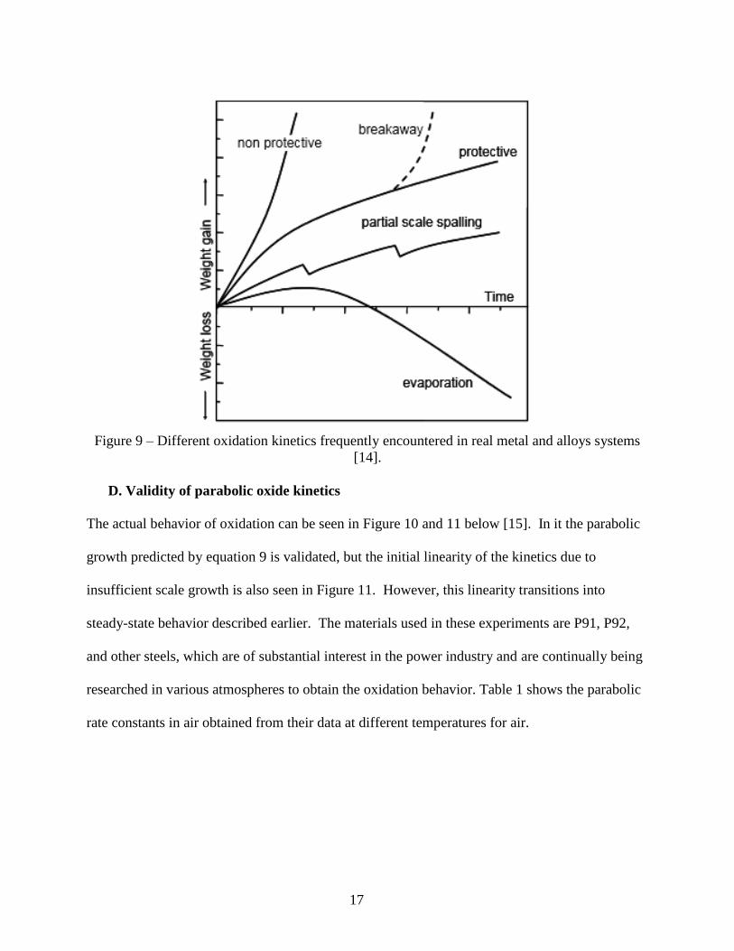
17
Figure 9 – Different oxidation kinetics frequently encountered in real metal and alloys systems
[14].
D. Validity of parabolic oxide kinetics
The actual behavior of oxidation can be seen in Figure 10 and 11 below [15]. In it the parabolic
growth predicted by equation 9 is validated, but the initial linearity of the kinetics due to
insufficient scale growth is also seen in Figure 11. However, this linearity transitions into
steady-state behavior described earlier. The materials used in these experiments are P91, P92,
and other steels, which are of substantial interest in the power industry and are continually being
researched in various atmospheres to obtain the oxidation behavior. Table 1 shows the parabolic
rate constants in air obtained from their data at different temperatures for air.
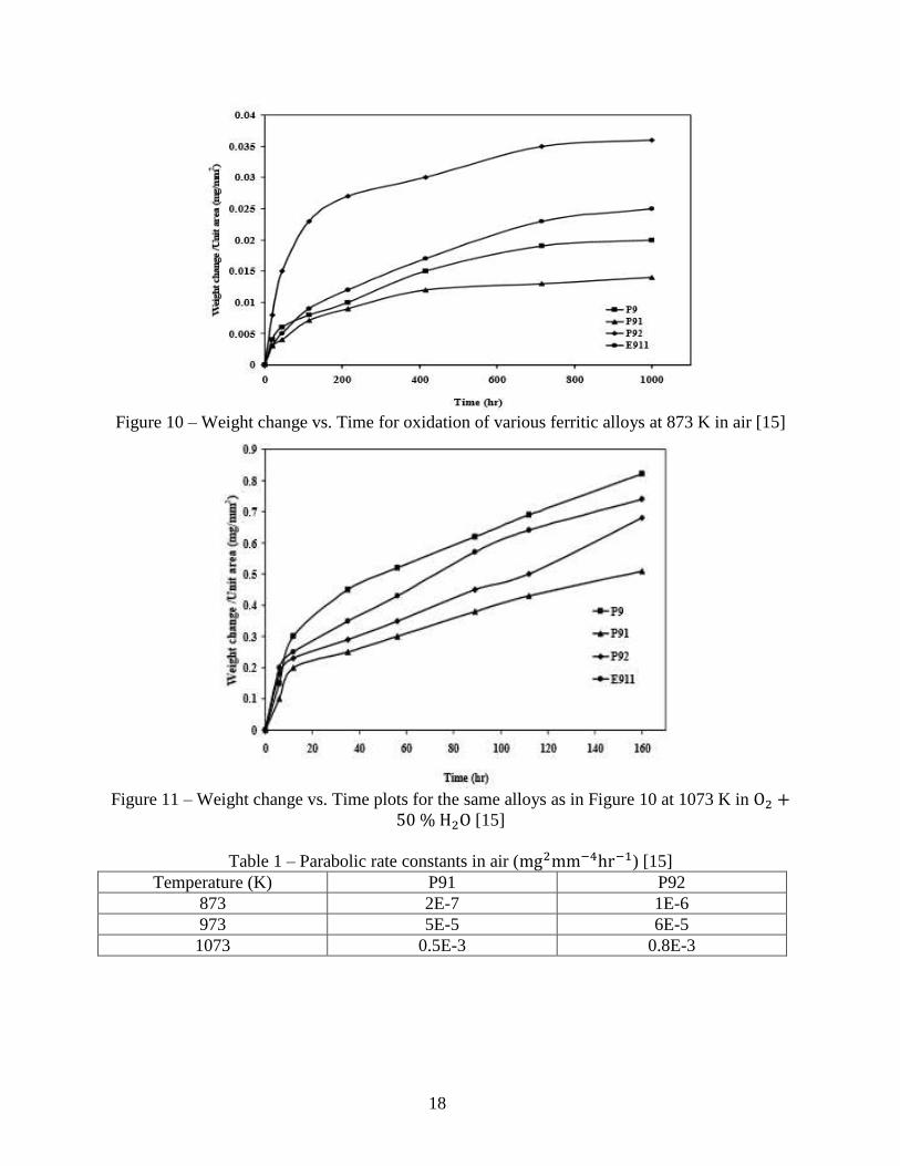
18
Figure 10 – Weight change vs. Time for oxidation of various ferritic alloys at 873 K in air [15]
Figure 11 – Weight change vs. Time plots for the same alloys as in Figure 10 at 1073 K in O2 +
50 % H2O [15]
Table 1 – Parabolic rate constants in air (mg2mm−4hr−1) [15]
Temperature (K) P91 P92
873 2E-7 1E-6
973 5E-5 6E-5
1073 0.5E-3 0.8E-3
19
E. Using Oxide Growth Kinetics to Determine Crack Growth Rates
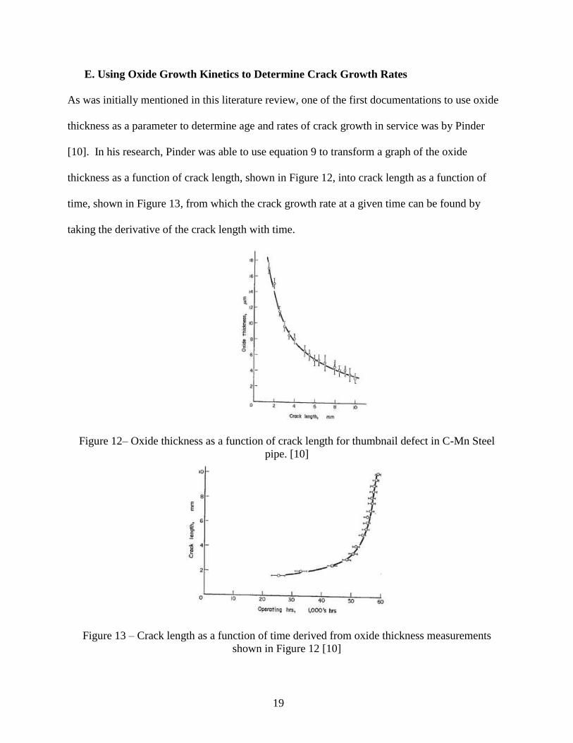
As was initially mentioned in this literature review, one of the first documentations to use oxide
thickness as a parameter to determine age and rates of crack growth in service was by Pinder
[10]. In his research, Pinder was able to use equation 9 to transform a graph of the oxide
thickness as a function of crack length, shown in Figure 12, into crack length as a function of
time, shown in Figure 13, from which the crack growth rate at a given time can be found by
taking the derivative of the crack length with time.
Figure 12– Oxide thickness as a function of crack length for thumbnail defect in C-Mn Steel
pipe. [10]
Figure 13 – Crack length as a function of time derived from oxide thickness measurements
shown in Figure 12 [10]

20
The first step in outlining the experiment process of finding if oxide thickness kinetics on crack
surfaces can be used to predict crack growth rates was to choose a material. For this study, P91
steel was chosen from a previously conducted study on creep-fatigue crack growth rates as the
test material because of the accessibility to crack length versus time data. Also, P91 steel chosen
is in extensive use in high temperature components making the study highly technologically
relevant.
21
IV. Experimental Setup and Process
The experimental setup and process can be divided into seven sub-steps as follows:
1. Experimental Setup
i. Test Material Selection
ii. Specimen Design and Machining
2. Experimental Process
i. Sample Preparation
ii. Pre-Oxidation Weighing
iii. Oxidation of the Samples in Furnace
iv. Post-Oxidation Weighing
v. Application of Protective Ni Coating
vi. Measurement of Oxide Thickness
This methodology was chosen in accordance with the study by Mathiazhagan and Khanna[15]
who also presented results on the same class of materials (ASTM Grade P91).
A. Experimental Setup
A.i) Test Material Chosen for Experiments
The test material chosen is a modified 9% chromium (Cr)-1% molybdenum (Mo) steel that is
designated by the ASTM as grade P91 steel wherein the prefix P denotes piping application [16].
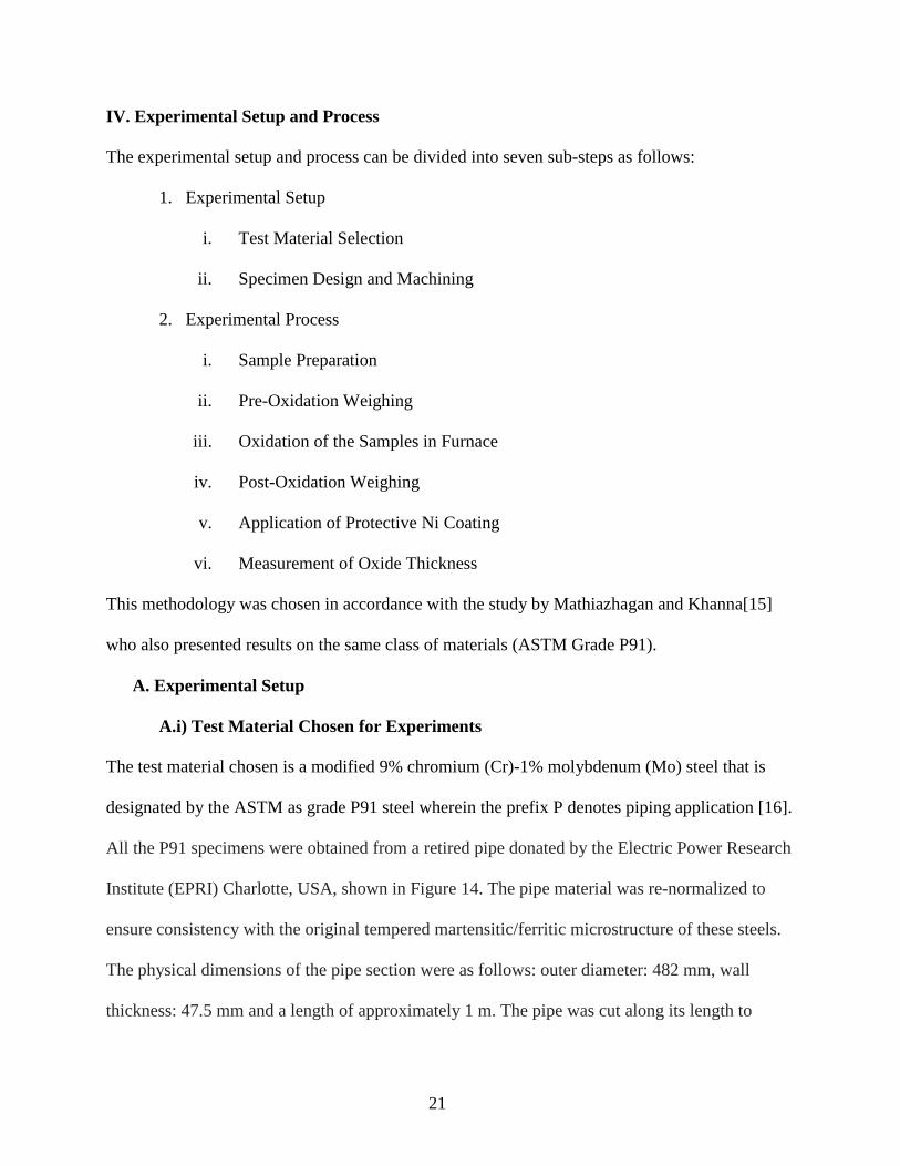
All the P91 specimens were obtained from a retired pipe donated by the Electric Power Research
Institute (EPRI) Charlotte, USA, shown in Figure 14. The pipe material was re-normalized to
ensure consistency with the original tempered martensitic/ferritic microstructure of these steels.
The physical dimensions of the pipe section were as follows: outer diameter: 482 mm, wall
thickness: 47.5 mm and a length of approximately 1 m. The pipe was cut along its length to
22
obtain approximately 3 equal sections. The 3 cut segments were respectively labeled as sections
1, 2 and 3 and only the cut Sections 2 and 3 were used in round robins (RRs) conducted to verify
test standards for creep-fatigue crack initiation and for crack propagation. A comprehensive
collection of all the specimen drawings and machining layouts, along with other test matrix
details, used for the current RR is provided in a recent EPRI report and publication [17]. The
chemical composition of P91 steel used in the RR testing in weight% is given in Table 2.
Figure 14- Picture of the pipe from which the test material for the program was extracted.
Table 2 – Chemical composition of test material (in weight %)[17]
C Si Mn P S Ni Cr Mo As V Nb Al Cu N Sb,
Sn Fe
0.11 0.31 0.45 0.011 0.009 0.19 8.22 0.94 0.005 0.21 0.07 0.006 0.16 0.039 0.001 Bal.
Tensile tests, creep deformation, and rupture tests on P91 steel were conducted at 6250C to fully
characterize the material and the results were reported in reference [17].
A.ii) Sample Design and Creation
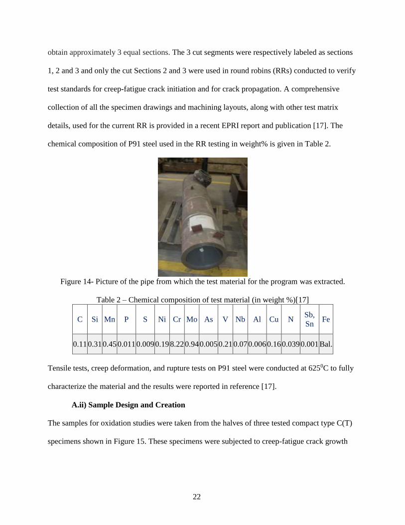
The samples for oxidation studies were taken from the halves of three tested compact type C(T)
specimens shown in Figure 15. These specimens were subjected to creep-fatigue crack growth
23
testing as part of the round robin program in support of ASTM Standard E2760-10 [9]. Further
details of the material and its mechanical properties can be found in reference 17.
Figure 15 - Picture of a tested creep-fatigue crack growth specimen used for machining the
oxidation samples.
Seventeen rectangular oxidation samples (six from each specimen half) with dimensions of
20mm x 10mm x 5mm were machined using the both halves from three tested creep-fatigue
crack growth specimens, shown in Figure 16. In-plane sample dimensions were similar to
samples used by Mathiazhagan and Khanna but the thickness of our specimens was 5 mm while
the other study used a sample thickness of 10 mm. A 3 mm diameter through-hole in the sample
was chosen to mount the samples in the furnace.
Oxidized surface where creep-fatigue crack growth occurred during testing

24
Figure 16 – CAD of Oxidation Samples
B. Experimental Process
B.i) Preparation of Oxidation Samples
The technique for preparation of oxidation samples was similar to the technique used by
Mathiazhagan and Khanna [15] with some differences. Mathiazhagan and Khanna’s samples
were prepared by mechanically polishing up to grit of 800 followed by ultrasonically cleaning
with acetone and allowing time to dry before the oxidation test. The end results were data points
collected of weight gain of the samples as a function of time of exposure and the test
temperature. The polishing process in our experiments consisted of a progression from a coarser
to finer grit finishing at a grit number of 800 without an ultrasonic cleaning with acetone. The
grit sequence was:
25
1. Start with 200 Grit Paper
2. Move to 400 Grit paper
3. Move to 800 Grit Paper
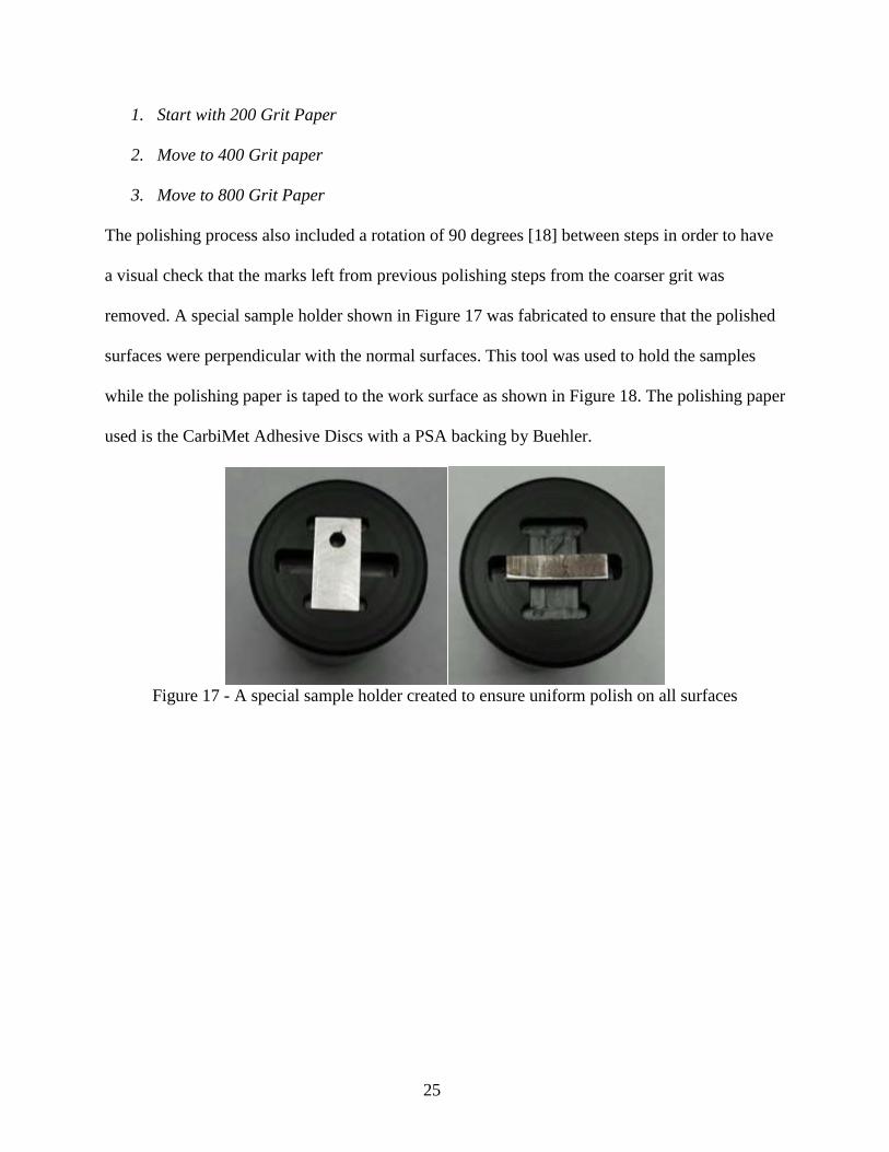
The polishing process also included a rotation of 90 degrees [18] between steps in order to have
a visual check that the marks left from previous polishing steps from the coarser grit was
removed. A special sample holder shown in Figure 17 was fabricated to ensure that the polished
surfaces were perpendicular with the normal surfaces. This tool was used to hold the samples
while the polishing paper is taped to the work surface as shown in Figure 18. The polishing paper
used is the CarbiMet Adhesive Discs with a PSA backing by Buehler.
Figure 17 - A special sample holder created to ensure uniform polish on all surfaces
26
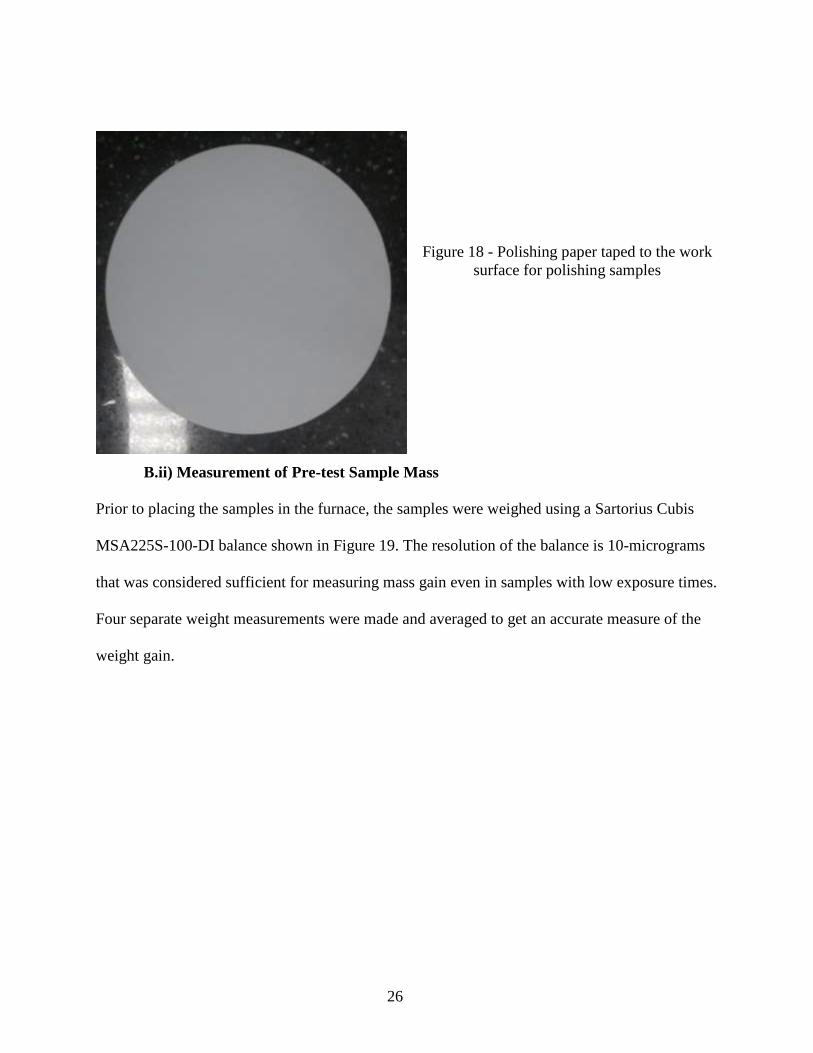
Figure 18 - Polishing paper taped to the work
surface for polishing samples
B.ii) Measurement of Pre-test Sample Mass
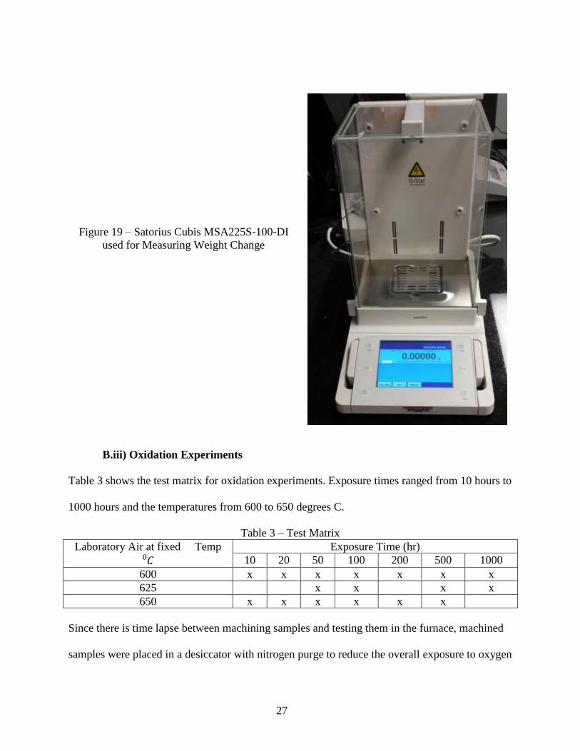
Prior to placing the samples in the furnace, the samples were weighed using a Sartorius Cubis
MSA225S-100-DI balance shown in Figure 19. The resolution of the balance is 10-micrograms
that was considered sufficient for measuring mass gain even in samples with low exposure times.
Four separate weight measurements were made and averaged to get an accurate measure of the
weight gain.
27
Figure 19 – Satorius Cubis MSA225S-100-DI
used for Measuring Weight Change
B.iii) Oxidation Experiments
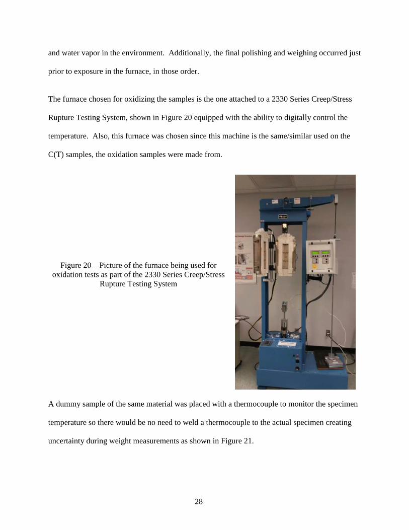
Table 3 shows the test matrix for oxidation experiments. Exposure times ranged from 10 hours to
1000 hours and the temperatures from 600 to 650 degrees C.
Table 3 – Test Matrix
Laboratory Air at fixed Temp
𝐶𝑖0
Exposure Time (hr)
10 20 50 100 200 500 1000
600 x x x x x x x
625 x x x x
650 x x x x x x
Since there is time lapse between machining samples and testing them in the furnace, machined
samples were placed in a desiccator with nitrogen purge to reduce the overall exposure to oxygen
28
and water vapor in the environment. Additionally, the final polishing and weighing occurred just
prior to exposure in the furnace, in those order.
The furnace chosen for oxidizing the samples is the one attached to a 2330 Series Creep/Stress
Rupture Testing System, shown in Figure 20 equipped with the ability to digitally control the
temperature. Also, this furnace was chosen since this machine is the same/similar used on the
C(T) samples, the oxidation samples were made from.
Figure 20 – Picture of the furnace being used for
oxidation tests as part of the 2330 Series Creep/Stress
Rupture Testing System
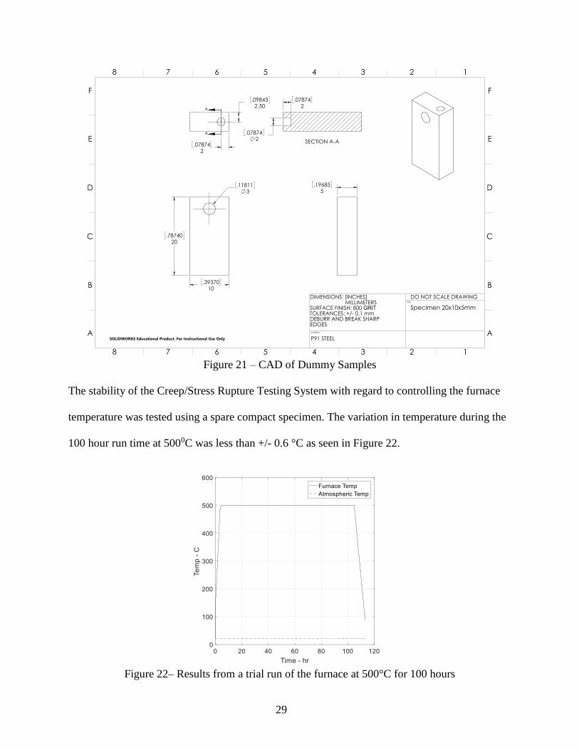
A dummy sample of the same material was placed with a thermocouple to monitor the specimen
temperature so there would be no need to weld a thermocouple to the actual specimen creating
uncertainty during weight measurements as shown in Figure 21.
29
Figure 21 – CAD of Dummy Samples
The stability of the Creep/Stress Rupture Testing System with regard to controlling the furnace
temperature was tested using a spare compact specimen. The variation in temperature during the
100 hour run time at 5000C was less than +/- 0.6 °C as seen in Figure 22.
Figure 22– Results from a trial run of the furnace at 500°C for 100 hours
30
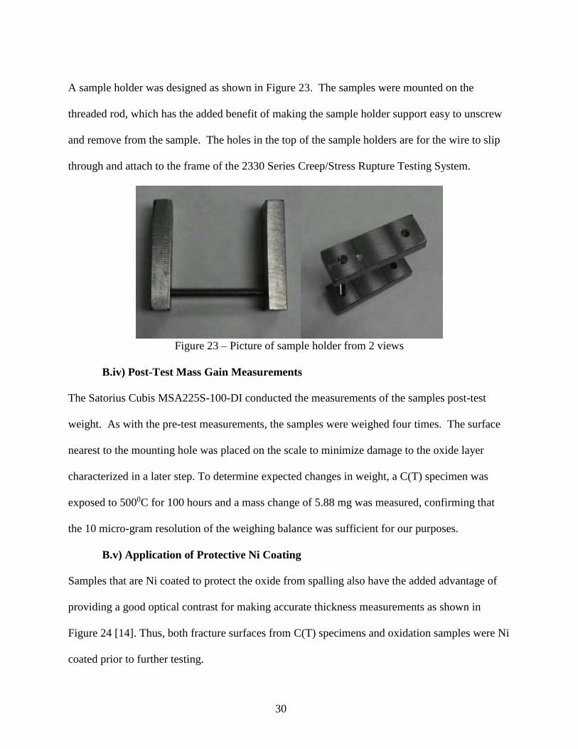
A sample holder was designed as shown in Figure 23. The samples were mounted on the
threaded rod, which has the added benefit of making the sample holder support easy to unscrew
and remove from the sample. The holes in the top of the sample holders are for the wire to slip
through and attach to the frame of the 2330 Series Creep/Stress Rupture Testing System.
Figure 23 – Picture of sample holder from 2 views
B.iv) Post-Test Mass Gain Measurements
The Satorius Cubis MSA225S-100-DI conducted the measurements of the samples post-test
weight. As with the pre-test measurements, the samples were weighed four times. The surface
nearest to the mounting hole was placed on the scale to minimize damage to the oxide layer
characterized in a later step. To determine expected changes in weight, a C(T) specimen was
exposed to 5000C for 100 hours and a mass change of 5.88 mg was measured, confirming that
the 10 micro-gram resolution of the weighing balance was sufficient for our purposes.
B.v) Application of Protective Ni Coating
Samples that are Ni coated to protect the oxide from spalling also have the added advantage of
providing a good optical contrast for making accurate thickness measurements as shown in
Figure 24 [14]. Thus, both fracture surfaces from C(T) specimens and oxidation samples were Ni
coated prior to further testing.
31
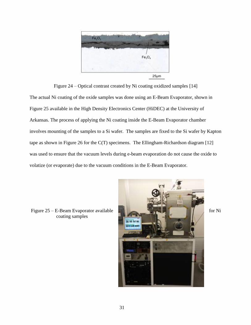
Figure 24 – Optical contrast created by Ni coating oxidized samples [14]
The actual Ni coating of the oxide samples was done using an E-Beam Evaporator, shown in
Figure 25 available in the High Density Electronics Center (HiDEC) at the University of
Arkansas. The process of applying the Ni coating inside the E-Beam Evaporator chamber
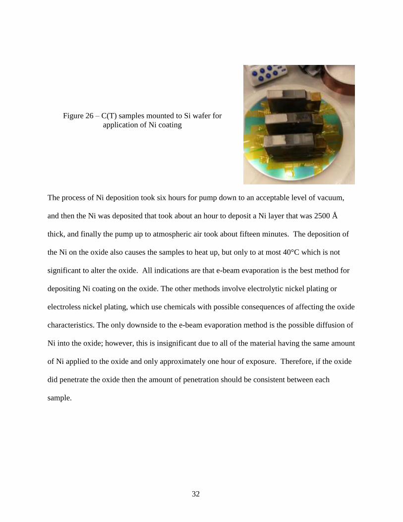
involves mounting of the samples to a Si wafer. The samples are fixed to the Si wafer by Kapton
tape as shown in Figure 26 for the C(T) specimens. The Ellingham-Richardson diagram [12]
was used to ensure that the vacuum levels during e-beam evaporation do not cause the oxide to
volatize (or evaporate) due to the vacuum conditions in the E-Beam Evaporator.
Figure 25 – E-Beam Evaporator available for Ni
coating samples
32
Figure 26 – C(T) samples mounted to Si wafer for
application of Ni coating
The process of Ni deposition took six hours for pump down to an acceptable level of vacuum,
and then the Ni was deposited that took about an hour to deposit a Ni layer that was 2500 Å
thick, and finally the pump up to atmospheric air took about fifteen minutes. The deposition of
the Ni on the oxide also causes the samples to heat up, but only to at most 40°C which is not
significant to alter the oxide. All indications are that e-beam evaporation is the best method for
depositing Ni coating on the oxide. The other methods involve electrolytic nickel plating or
electroless nickel plating, which use chemicals with possible consequences of affecting the oxide
characteristics. The only downside to the e-beam evaporation method is the possible diffusion of
Ni into the oxide; however, this is insignificant due to all of the material having the same amount
of Ni applied to the oxide and only approximately one hour of exposure. Therefore, if the oxide
did penetrate the oxide then the amount of penetration should be consistent between each
sample.
33
B.vi) Measurement of Oxide Profiles and Thicknesses
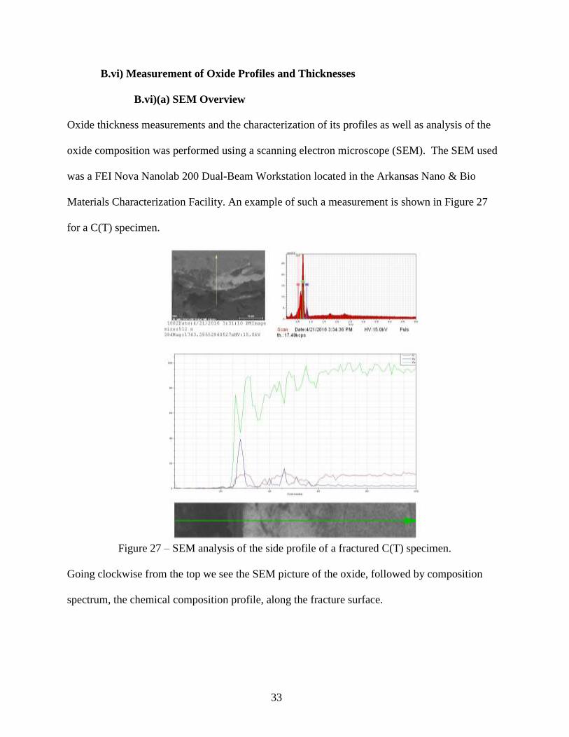
B.vi)(a) SEM Overview
Oxide thickness measurements and the characterization of its profiles as well as analysis of the
oxide composition was performed using a scanning electron microscope (SEM). The SEM used
was a FEI Nova Nanolab 200 Dual-Beam Workstation located in the Arkansas Nano & Bio
Materials Characterization Facility. An example of such a measurement is shown in Figure 27
for a C(T) specimen.
Figure 27 – SEM analysis of the side profile of a fractured C(T) specimen.
Going clockwise from the top we see the SEM picture of the oxide, followed by composition
spectrum, the chemical composition profile, along the fracture surface.
34
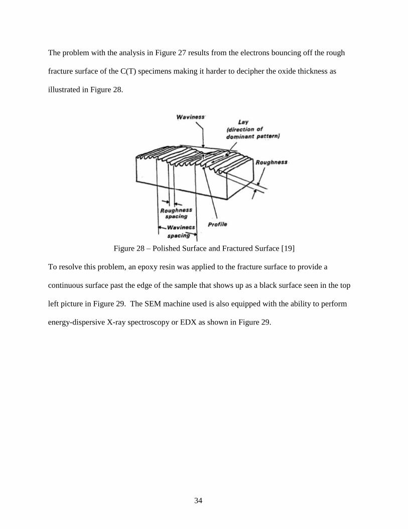
The problem with the analysis in Figure 27 results from the electrons bouncing off the rough
fracture surface of the C(T) specimens making it harder to decipher the oxide thickness as
illustrated in Figure 28.
Figure 28 – Polished Surface and Fractured Surface [19]
To resolve this problem, an epoxy resin was applied to the fracture surface to provide a
continuous surface past the edge of the sample that shows up as a black surface seen in the top
left picture in Figure 29. The SEM machine used is also equipped with the ability to perform
energy-dispersive X-ray spectroscopy or EDX as shown in Figure 29.
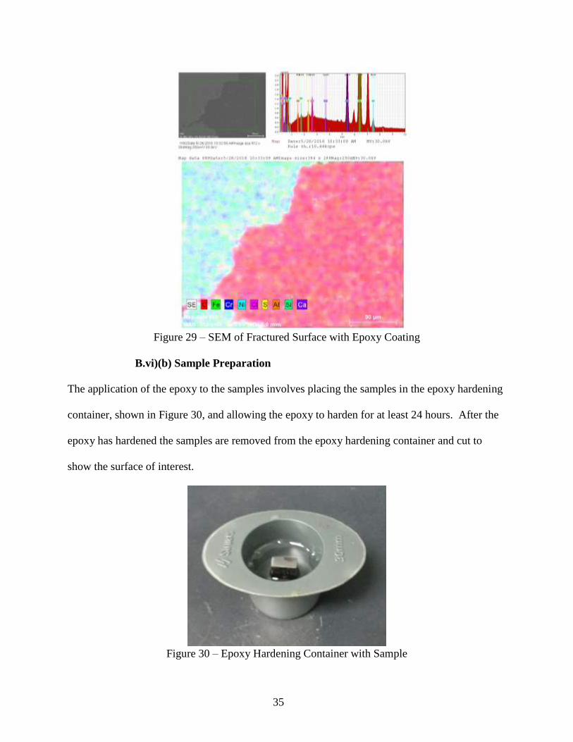
35
Figure 29 – SEM of Fractured Surface with Epoxy Coating
B.vi)(b) Sample Preparation
The application of the epoxy to the samples involves placing the samples in the epoxy hardening
container, shown in Figure 30, and allowing the epoxy to harden for at least 24 hours. After the
epoxy has hardened the samples are removed from the epoxy hardening container and cut to
show the surface of interest.
Figure 30 – Epoxy Hardening Container with Sample
36
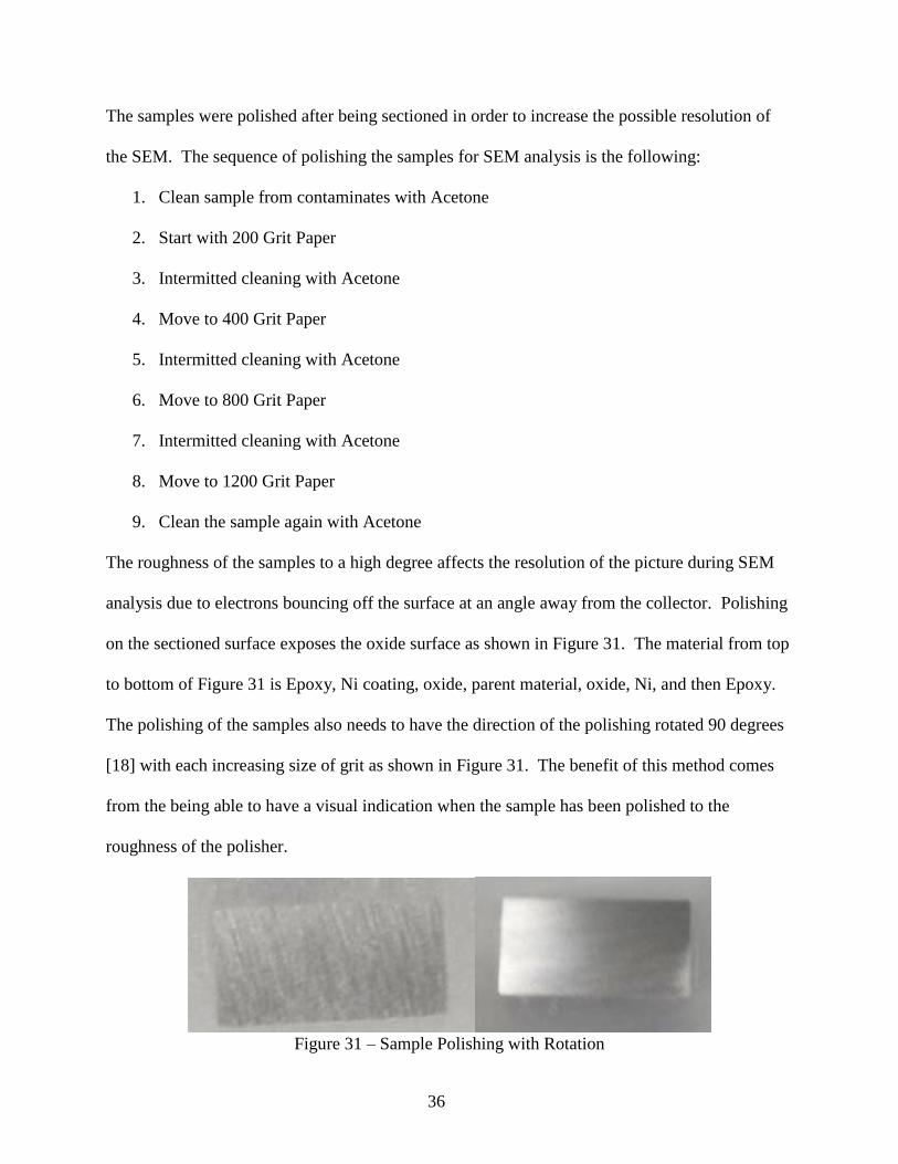
The samples were polished after being sectioned in order to increase the possible resolution of
the SEM. The sequence of polishing the samples for SEM analysis is the following:
1. Clean sample from contaminates with Acetone
2. Start with 200 Grit Paper
3. Intermitted cleaning with Acetone
4. Move to 400 Grit Paper
5. Intermitted cleaning with Acetone
6. Move to 800 Grit Paper
7. Intermitted cleaning with Acetone
8. Move to 1200 Grit Paper
9. Clean the sample again with Acetone
The roughness of the samples to a high degree affects the resolution of the picture during SEM
analysis due to electrons bouncing off the surface at an angle away from the collector. Polishing
on the sectioned surface exposes the oxide surface as shown in Figure 31. The material from top
to bottom of Figure 31 is Epoxy, Ni coating, oxide, parent material, oxide, Ni, and then Epoxy.
The polishing of the samples also needs to have the direction of the polishing rotated 90 degrees
[18] with each increasing size of grit as shown in Figure 31. The benefit of this method comes
from the being able to have a visual indication when the sample has been polished to the
roughness of the polisher.
Figure 31 – Sample Polishing with Rotation
37
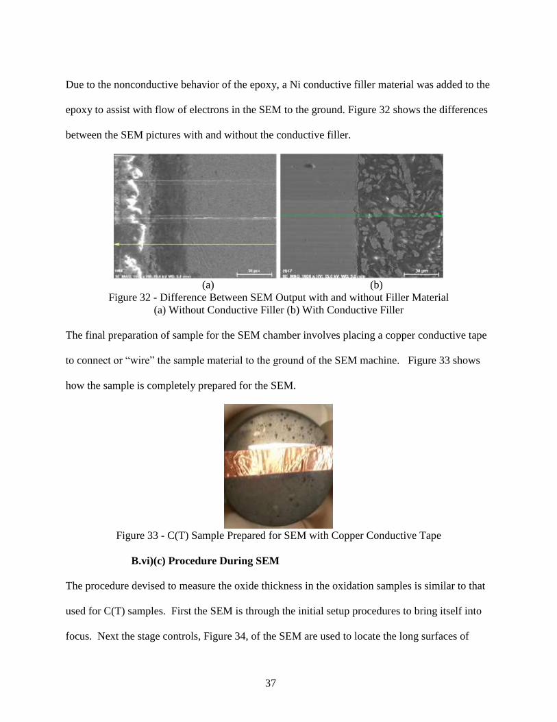
Due to the nonconductive behavior of the epoxy, a Ni conductive filler material was added to the
epoxy to assist with flow of electrons in the SEM to the ground. Figure 32 shows the differences
between the SEM pictures with and without the conductive filler.
(a) (b)
Figure 32 - Difference Between SEM Output with and without Filler Material
(a) Without Conductive Filler (b) With Conductive Filler
The final preparation of sample for the SEM chamber involves placing a copper conductive tape
to connect or “wire” the sample material to the ground of the SEM machine. Figure 33 shows
how the sample is completely prepared for the SEM.
Figure 33 - C(T) Sample Prepared for SEM with Copper Conductive Tape
B.vi)(c) Procedure During SEM
The procedure devised to measure the oxide thickness in the oxidation samples is similar to that
used for C(T) samples. First the SEM is through the initial setup procedures to bring itself into
focus. Next the stage controls, Figure 34, of the SEM are used to locate the long surfaces of
38
interest for both the oxidized samples and the C(T) specimens, which is the top surface of Figure
33 for a C(T) sample.
The next step is dependent on if it is the oxidized sample or a C(T) sample being analyzed. For
the oxide samples, the next steps were devised to collect data as near to the center of the
sample’s oxide edges to minimize influence from the corners. The SEM stage control has the
capability of moving to points on the surface of the sample with increments down to 0.0001 mm
as shown in Figure 34.
Figure 34 – SEM Sample Stage Movement Control
The center point can be found by measuring the location using the x and y stage movement
controls referenced to the two corners. The final step for the oxide sample is to take nine EDX
measurements with four points taken in 0.5 mm increments above and below the center point of
the sample.
39
The process of measuring the oxide thickness after finding the surface of interest for the C(T)
sample involves locating the beginning and end points of the creep-fatigue crack surface. The
oxide thickness between the beginning and end points of creep-fatigue crack growth were
measured in 0.5 mm increments using the EDX.
B.vi)(d) Procedure for Analyzing SEM Photomicrographs
The analysis of the SEM photomicrographs is done in MATLAB© using it’s imtool. The
necessary steps to open the image in the imtool are shown in Figure 35, which is achieved by
calling the imtool as a function with the input of the image file to analysis.
Figure 35 - MATLAB© Command Window to Pull Images into imtool
The result of Figure 35 is a new window shown in Figure 36. Figure 36 shows the EDX output
of the SEM, which is a map of location of oxygen on the sample’s surface. The difference in
brightness or luminosity of Figure 36 is an indication of the oxygen content at a location.
Therefore by using the difference in luminosity of Figure 36 the oxide is easy to find, being the
lighter green content in the center. Another feature of the imtool is an icon on the imtool toolbar
that allows the measurement of pixel distance as shown in Figure 37. Once clicked on, the
40
cursor turns into a plus sign that allows you to hold and drag it to the opposite side of the oxide
to show the pixel distance between the edges of the oxide. The output a single distance
measurement is shown in Figure 38.
Figure 36 - imtool on an EDX SEM Image
Figure 37 - imtool Toolbar
Figure 38 - Zoomed in Output of Measure Distance Icon
The advantage of this process comes from finding the pixel to length ratio from the scale in the
bottom right corner of Figure 36. Using the pixel to length ratio the pixel distance of multiple
Measure distance icon
41
measurements, as shown in Figure 39, can be converted and averaged to find the oxide thickness
at this location.
Figure 39 - Output for One Location using MATLAB©’s imtool
The only downside to this method is this is a manual edge detection method that relies on the
user to click and drag to find the distance. To try and elevate this in a more automated approach,
MATLAB©’s edge detection was used to alleviate this. Figure 66 shows an output applied using
different tolerances. The results of using MATLAB©’s edge detection where not satisfactory to
create a method of finding the distance between points and was therefore abandoned. However,
if successful edge detection software was applied ability and speed of calculating the oxide
thickness should increase.
42
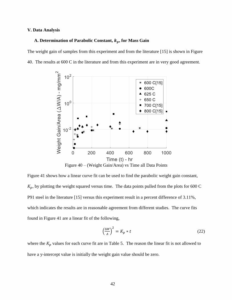
V. Data Analysis
A. Determination of Parabolic Constant, 𝒌𝒑, for Mass Gain
The weight gain of samples from this experiment and from the literature [15] is shown in Figure
40. The results at 600 C in the literature and from this experiment are in very good agreement.
Figure 40 – (Weight Gain/Area) vs Time all Data Points
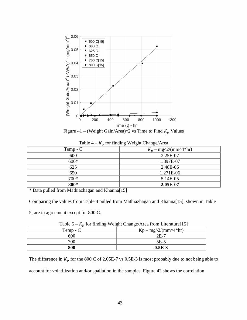
Figure 41 shows how a linear curve fit can be used to find the parabolic weight gain constant,
𝐾𝑝, by plotting the weight squared versus time. The data points pulled from the plots for 600 C
P91 steel in the literature [15] versus this experiment result in a percent difference of 3.11%,
which indicates the results are in reasonable agreement from different studies. The curve fits
found in Figure 41 are a linear fit of the following,
(∆𝑊
𝐴)
2
= 𝐾𝑝 ∗ 𝑡 (22)
where the 𝐾𝑝 values for each curve fit are in Table 5. The reason the linear fit is not allowed to
have a y-intercept value is initially the weight gain value should be zero.
43
Figure 41 – (Weight Gain/Area)^2 vs Time to Find 𝐾𝑝 Values
Table 4 – 𝐾𝑝 for finding Weight Change/Area
Temp - C 𝐾𝑝 – mg^2/(mm^4*hr)
600 2.25E-07
600* 1.897E-07
625 2.48E-06
650 1.271E-06
700* 5.14E-05
800* 2.05E-07
* Data pulled from Mathiazhagan and Khanna[15]
Comparing the values from Table 4 pulled from Mathiazhagan and Khanna[15], shown in Table
5, are in agreement except for 800 C.
Table 5 – 𝐾𝑝 for finding Weight Change/Area from Literature[15]
Temp - C Kp – mg^2/(mm^4*hr)
600 2E-7
700 5E-5
800 0.5E-3
The difference in 𝐾𝑝 for the 800 C of 2.05E-7 vs 0.5E-3 is most probably due to not being able to
account for volatilization and/or spallation in the samples. Figure 42 shows the correlation
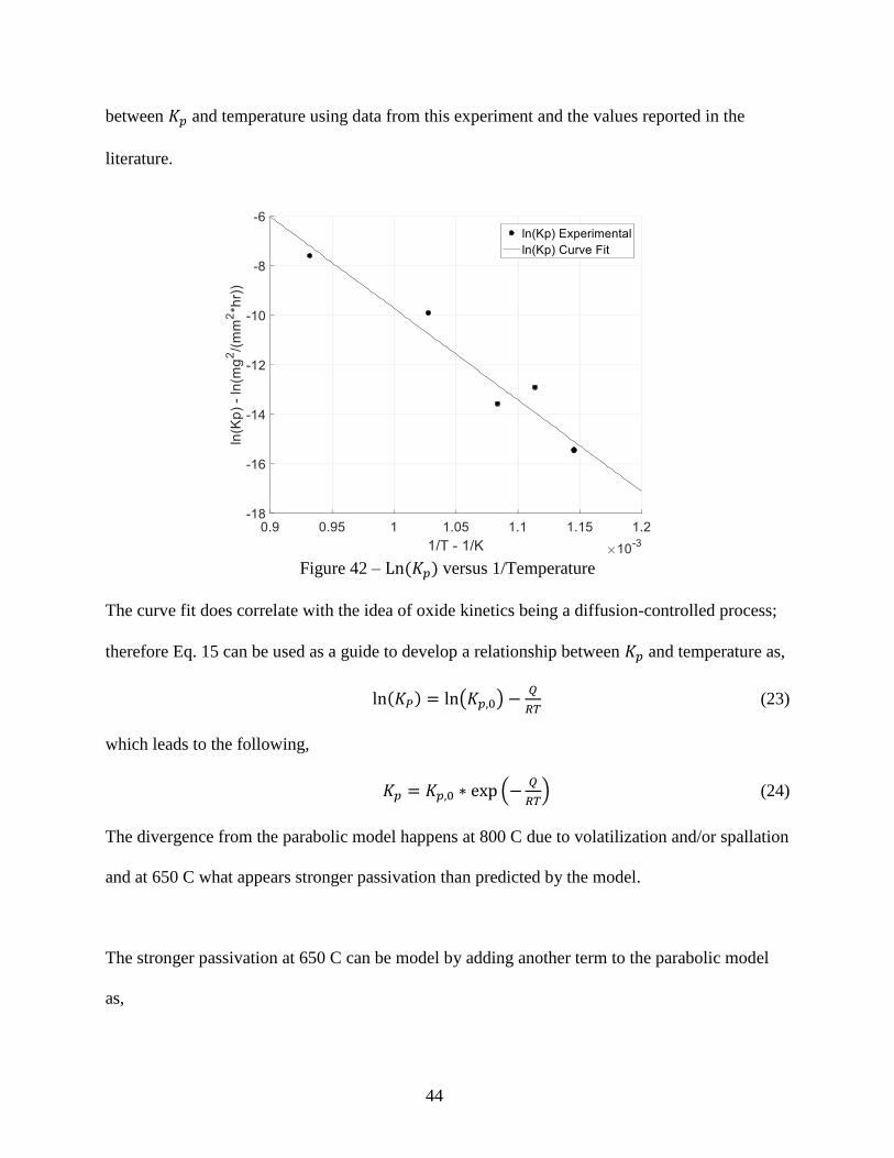
44
between 𝐾𝑝 and temperature using data from this experiment and the values reported in the
literature.
Figure 42 – Ln (𝐾𝑝) versus 1/Temperature
The curve fit does correlate with the idea of oxide kinetics being a diffusion-controlled process;
therefore Eq. 15 can be used as a guide to develop a relationship between 𝐾𝑝 and temperature as,
ln(𝐾𝑃) = ln(𝐾𝑝,0) −𝑄
𝑅𝑇 (23)
which leads to the following,
𝐾𝑝 = 𝐾𝑝,0 ∗ exp (−𝑄
𝑅𝑇) (24)
The divergence from the parabolic model happens at 800 C due to volatilization and/or spallation
and at 650 C what appears stronger passivation than predicted by the model.
The stronger passivation at 650 C can be model by adding another term to the parabolic model
as,
45
∆𝑊
𝐴= √𝐾𝑝 ∗ 𝑡 + 𝑐0 ∗ 𝑡𝑐1 (25)
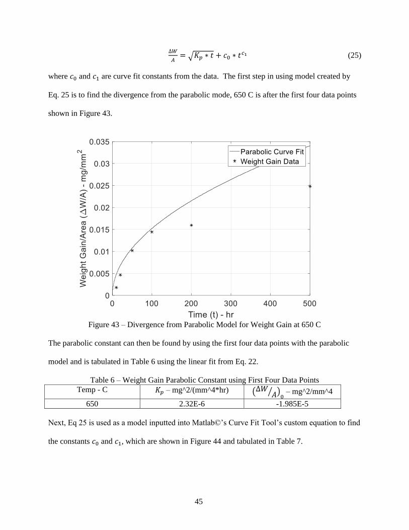
where 𝑐0 and 𝑐1 are curve fit constants from the data. The first step in using model created by
Eq. 25 is to find the divergence from the parabolic mode, 650 C is after the first four data points
shown in Figure 43.
Figure 43 – Divergence from Parabolic Model for Weight Gain at 650 C
The parabolic constant can then be found by using the first four data points with the parabolic
model and is tabulated in Table 6 using the linear fit from Eq. 22.
Table 6 – Weight Gain Parabolic Constant using First Four Data Points
Temp - C 𝐾𝑝 – mg^2/(mm^4*hr) (∆𝑊𝐴⁄ )
0 – mg^2/mm^4
650 2.32E-6 -1.985E-5
Next, Eq 25 is used as a model inputted into Matlab©’s Curve Fit Tool’s custom equation to find
the constants 𝑐0 and 𝑐1, which are shown in Figure 44 and tabulated in Table 7.
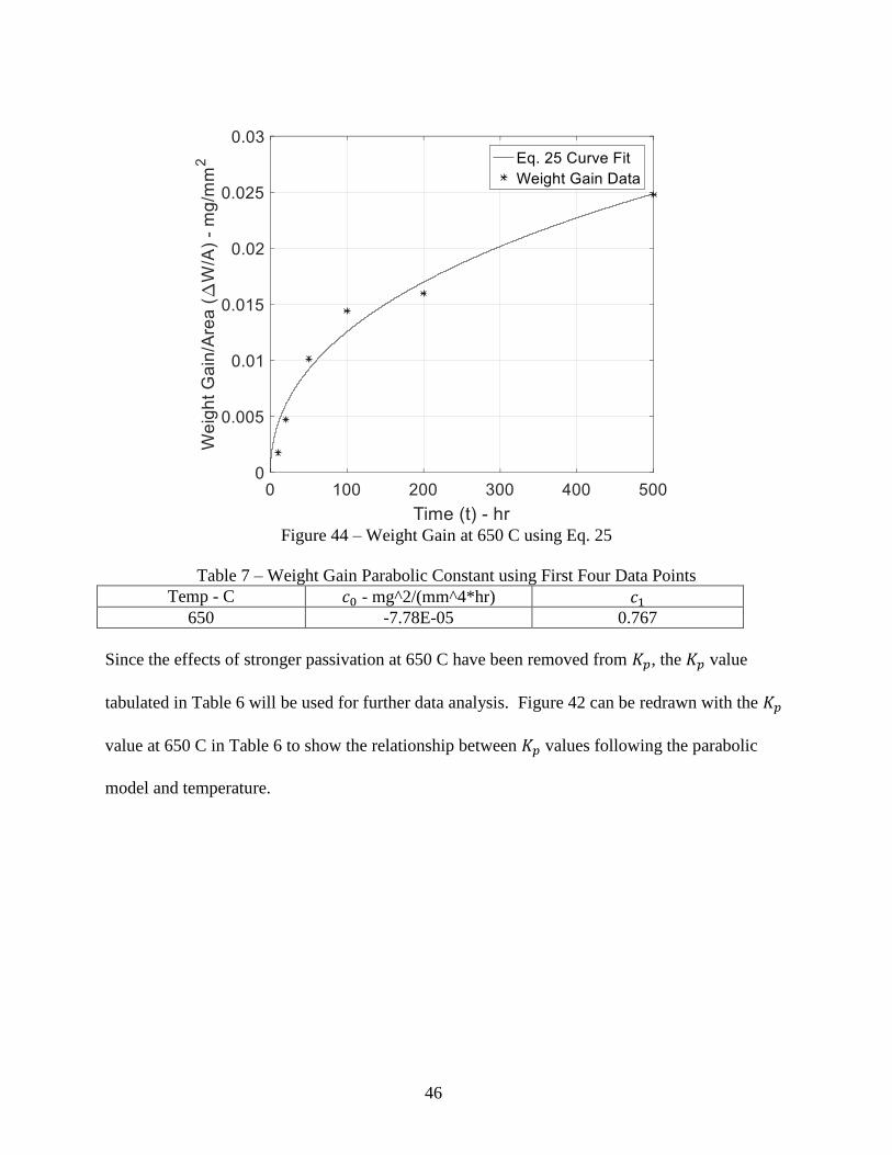
46
Figure 44 – Weight Gain at 650 C using Eq. 25
Table 7 – Weight Gain Parabolic Constant using First Four Data Points
Temp - C 𝑐0 - mg^2/(mm^4*hr) 𝑐1
650 -7.78E-05 0.767
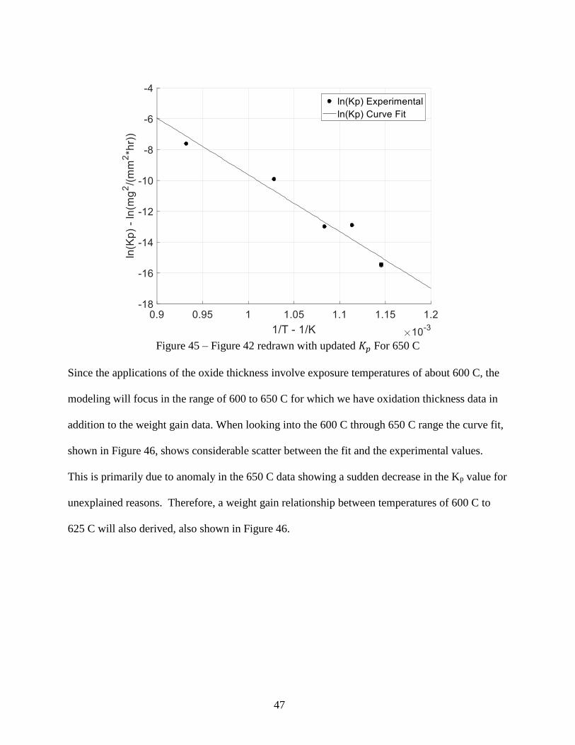
Since the effects of stronger passivation at 650 C have been removed from 𝐾𝑝, the 𝐾𝑝 value
tabulated in Table 6 will be used for further data analysis. Figure 42 can be redrawn with the 𝐾𝑝
value at 650 C in Table 6 to show the relationship between 𝐾𝑝 values following the parabolic
model and temperature.
47
Figure 45 – Figure 42 redrawn with updated 𝐾𝑝 For 650 C
Since the applications of the oxide thickness involve exposure temperatures of about 600 C, the
modeling will focus in the range of 600 to 650 C for which we have oxidation thickness data in
addition to the weight gain data. When looking into the 600 C through 650 C range the curve fit,
shown in Figure 46, shows considerable scatter between the fit and the experimental values.
This is primarily due to anomaly in the 650 C data showing a sudden decrease in the Kp value for
unexplained reasons. Therefore, a weight gain relationship between temperatures of 600 C to
625 C will also derived, also shown in Figure 46.
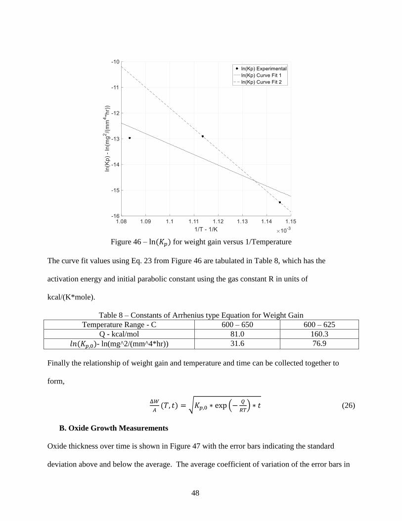
48
Figure 46 – ln (𝐾𝑝) for weight gain versus 1/Temperature
The curve fit values using Eq. 23 from Figure 46 are tabulated in Table 8, which has the
activation energy and initial parabolic constant using the gas constant R in units of
kcal/(K*mole).
Table 8 – Constants of Arrhenius type Equation for Weight Gain
Temperature Range - C 600 – 650 600 – 625
Q - kcal/mol 81.0 160.3
𝑙𝑛(𝐾𝑝,0)- ln(mg^2/(mm^4*hr)) 31.6 76.9
Finally the relationship of weight gain and temperature and time can be collected together to
form,
Δ𝑊
𝐴(𝑇, 𝑡) = √𝐾𝑝,0 ∗ exp (−
𝑄
𝑅𝑇) ∗ 𝑡 (26)
B. Oxide Growth Measurements
Oxide thickness over time is shown in Figure 47 with the error bars indicating the standard
deviation above and below the average. The average coefficient of variation of the error bars in
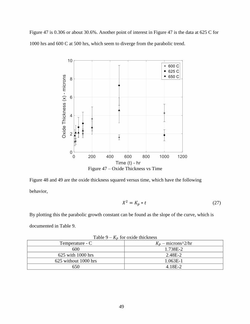
49
Figure 47 is 0.306 or about 30.6%. Another point of interest in Figure 47 is the data at 625 C for
1000 hrs and 600 C at 500 hrs, which seem to diverge from the parabolic trend.
Figure 47 – Oxide Thickness vs Time
Figure 48 and 49 are the oxide thickness squared versus time, which have the following
behavior,
𝑋2 = 𝐾𝑝 ∗ 𝑡 (27)
By plotting this the parabolic growth constant can be found as the slope of the curve, which is
documented in Table 9.
Table 9 – 𝐾𝑃 for oxide thickness
Temperature - C 𝐾𝑃 – microns^2/hr
600 1.738E-2
625 with 1000 hrs 2.48E-2
625 without 1000 hrs 1.063E-1
650 4.18E-2
50
Figure 48 – (Oxide Thickness)^2 vs Time
Figure 49 – (Oxide Thickness)^2 vs Time without 625 C 1000 hr
51
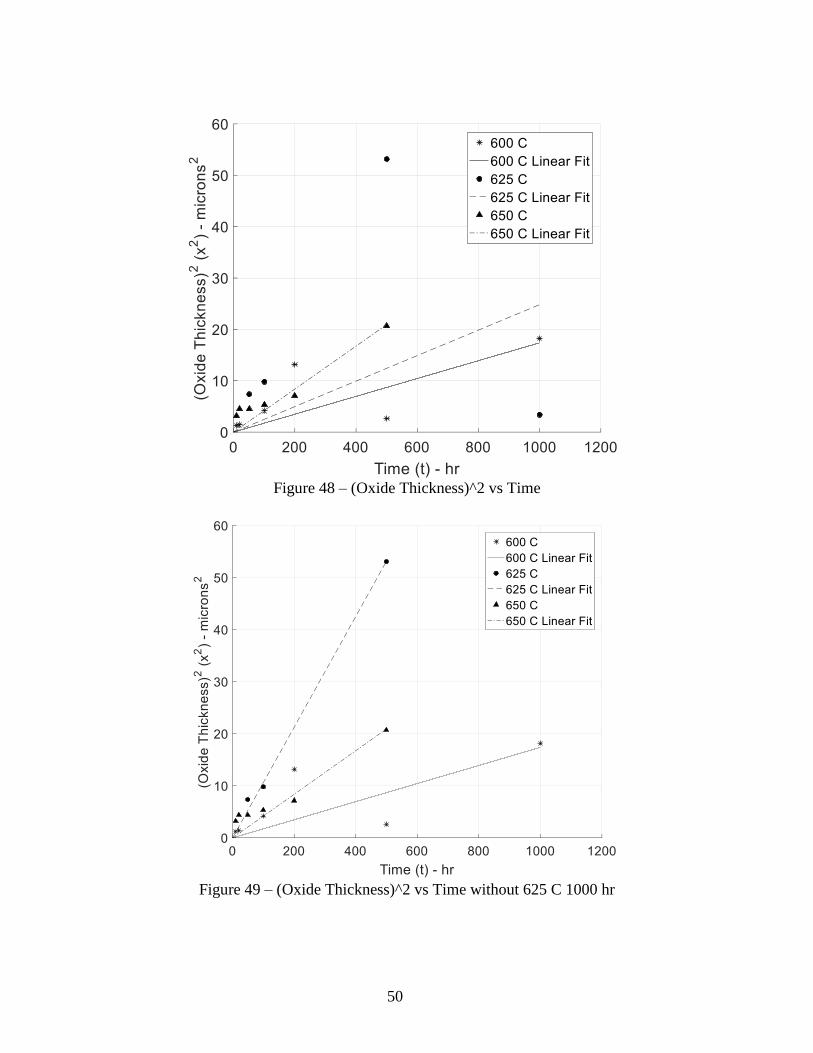
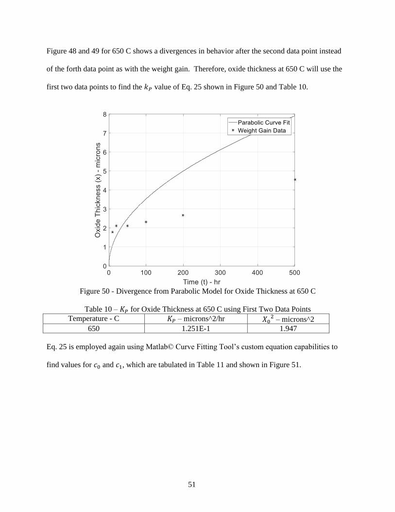
Figure 48 and 49 for 650 C shows a divergences in behavior after the second data point instead
of the forth data point as with the weight gain. Therefore, oxide thickness at 650 C will use the
first two data points to find the 𝑘𝑃 value of Eq. 25 shown in Figure 50 and Table 10.
Figure 50 - Divergence from Parabolic Model for Oxide Thickness at 650 C
Table 10 – 𝐾𝑃 for Oxide Thickness at 650 C using First Two Data Points
Temperature - C 𝐾𝑃 – microns^2/hr 𝑋02 – microns^2
650 1.251E-1 1.947
Eq. 25 is employed again using Matlab© Curve Fitting Tool’s custom equation capabilities to
find values for 𝑐0 and 𝑐1, which are tabulated in Table 11 and shown in Figure 51.
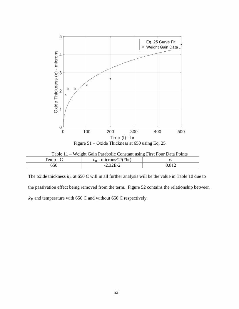
52
Figure 51 – Oxide Thickness at 650 using Eq. 25
Table 11 – Weight Gain Parabolic Constant using First Four Data Points
Temp - C 𝑐0 - microns^2/(*hr) 𝑐1
650 -2.32E-2 0.812
The oxide thickness 𝑘𝑃 at 650 C will in all further analysis will be the value in Table 10 due to
the passivation effect being removed from the term. Figure 52 contains the relationship between
𝑘𝑃 and temperature with 650 C and without 650 C respectively.

53
Figure 52 – ln(𝐾𝑃) for Oxide Thickness vs Temp^-1
The 𝐾𝑃 and temperature relationship in Figure 52 can be developed into a model exactly like Eq.
23 for Weight Gain leading to,
𝐾𝑝 = 𝐾𝑝,0 ∗ 𝑒𝑥𝑝 (−𝑄
𝑅𝑇) (28)
where the Q and 𝐾𝑝,0 values for oxide thickness are documented in Table 12.
Table 12 – Constants of Arrhenius type Equation for Oxide Thickness
Temperature Range - C 600 - 650 600 - 625
Q – kcal/mol 63.7 112.8
ln (𝐾𝑝,0) – microns^2/hr 32.9 61.0
The result relationship of oxide thickness with temperature and time is,
𝑥(𝑇, 𝑡) = √𝐾𝑝,0 ∗ exp (−𝑄
𝑅𝑇) ∗ 𝑡 (29)
Since all of the oxides are similar the activation energy found should be approximately equal, the
activation energy values in Table 8 should be approximately equal to the values in Table 12 with
the values comparison shown in Table 13.
54
Table 13 – Activation Energy Values
Q – kcal/mol
Figure 46, 600 – 650 C 81.0
Figure 46, 600 – 625 C 160.3
Figure 52, 600 – 650 C 63.7
Figure 52, 600 – 625 C 112.8
The activation energies tabulated in Table 14 show are activation energies found in Young’s
book[13]. The first two are from self-diffusion of Cr in a binary alloy of Cr-Fe(𝛾) and Cr-Fe(𝛼),
and the third value is the diffusion activation energy of Cr in 𝐶𝑟2𝑂3.
Table 14 – Comparable Activation Energy Values[13]
Type Q – kJ/mol
Self-diffusion of Cr in Cr-Fe(𝛾) 263.9
Self-diffusion of Cr in Cr-Fe(𝛼) 250.8
Diffusion of Cr in 𝐶𝑟2𝑂3 330
Upon inspection of the values in Table 14 and converting the values of Table 13, the correlation
between the activation energy of Figure 46 from 600 – 650 C and the Diffusion of Cr in 𝐶𝑟2𝑂3
along with the similarities between the activation energy of Figure 52 from 600 – 650 C and the
self-diffusion of Cr in Cr-Fe(𝛾) and Cr-Fe(𝛼) points towards using the activation energy in the
600 – 650 range can be seen in Table 15.
Table 15 – Comparison of Activation Energies
Type Q – kJ/mol
Self-diffusion of Cr in Cr-Fe(𝛾) [13] 263.9
Self-diffusion of Cr in Cr-Fe(𝛼) [13] 250.8
Figure 52, 600 – 650 C 267
Diffusion of Cr in 𝐶𝑟2𝑂3 [13] 330
Figure 46 – 600 – 650 C 339
Another implication of the activation energies of the temperature range 600 – 650 C being
similar is the assessment the controlling process being diffusion, which gives more credence to
the parabolic model. Since the activation energies between the Arrhenius oxidation and weight
gain models should be similar, the decision to use an average of the activation energies. Table
55
16 contains the averaging of the activation energies obtained from figure 46 and 52 with a
comparison of the averaging of the self-diffusion of Cr in Cr-Fe(𝛾) and diffusion of Cr in 𝐶𝑟2𝑂3.
Table 16 – Comparing Activation Energy Values
Q – kcal/mol Percent Difference - %
Figure 46, 600 – 650 C,WG 81.0 11.88%
Figure 52, 600 – 650 C,OT 63.7 12.72%
Average 72.4
Self-diffusion of Cr in Cr-
Fe(𝛾) [13] 63.1 11.79%
Diffusion of Cr in 𝐶𝑟2𝑂3
[13] 78.9 10.54%
Average 71.0
Comparing the averages of Table 16 results in a percent difference of less than 1%, and the
activation energy found from Figure 45 is also in agree with the 𝑄𝐴𝑉𝐺 found being 73 kcal/mol.
The weight change per area’s and oxide thickness’s activation energy being similar is important
due to the oxide thickness and weight should having the following relationship,
∆𝑥 ∝ (∆𝑊
𝐴) (30)
where ∆𝑥 is the increase in oxide and ∆𝑊
𝐴 is the weight change per surface area. The literature
[13] shows that the oxide and weight change per surface area relationship is the following,
𝑥 =1
16𝜌𝑠′ (
∆𝑊
𝐴) (31)
where 𝜌𝑠′ is the density of the scale or oxide in this case. The one-sixteenth constant in the
equation is derived from the following chemical equation,
𝑥
𝑦𝑀 +
1
2𝑂2 →
1
𝑦𝑀𝑥𝑂𝑦 (32)
where x and y are coefficients to balance out the chemical equation for a metal. The one-
sixteenth term comes from stoichiometric considerations during the oxidation reaction and can
be lumped into a single constant,
56
𝜌𝑠 = 16𝜌𝑠′ (33)
Therefore using Eq. 31 and 33, the density of the oxide can be modeled by,
𝜌𝑠 =1
𝑥(𝑇,𝑡)(
∆𝑊
𝐴(𝑇, 𝑡)) (34)
Inputting the oxide thickness and weight gain model into the above equations results in,
𝜌𝑠 = √𝐾𝑝,𝑂𝑊𝐺
𝐾𝑝,𝑂𝑂𝑇
∗ exp (𝑄𝑊𝐶−𝑄𝑂𝑇
𝑅𝑇) (35)
where WC signifies weight change and OT signifies oxide thickness. The 𝑄𝑊𝐶 and 𝑄𝑂𝑇 are both
taken as the average activation energy value derived from the two methods thus leading to,
𝜌𝑠 = √𝐾𝑝,𝑂𝑊𝐺
𝐾𝑝,𝑂𝑂𝑇
(36)
and,
𝑥(𝑡) =√𝐾𝑝,0𝑊𝐺
∗exp(−𝑄𝐴𝑉𝐺
𝑅𝑇)∗𝑡
𝜌𝑠 (37)
In order to achieve the above relationship using 𝑄𝐴𝑉𝐺 the 𝐾𝑝,0 values for weight gain and oxide
thickness will have to be retained using the 𝑄𝐴𝑉𝐺. The method chosen to find the 𝐾𝑝,0 is using
Curve Fitting Tool within Matlab because this allows the user to input custom equations. The
result of applying this method is seen in Figures 53 and 54, with the resulting curves tabulated in
Table 17.
57
Figure 53 – Weight Gain ln(Kp) using Qavg versus Qwg for 600, 625, and 650 C
Figure 54 – Oxide Thickness ln(Kp) using Qavg versus Qwg for 600, 625, and 650 C
58
Table 17 – Coefficients of Qavg Curve Fit
Figure 𝑎 = −𝑄
𝑅 𝑏 = ln (𝐾𝑝,0)
53 -3.64E4 26.8
54 -3.64E4 37.8
Using the ln (𝐾𝑝,0) term found by using Qavg the density constants, 𝜌𝑠 and 𝜌𝑠′, can now be found
by using Eq. 36.
Table 18 – Density Constant, 𝜌𝑠 and 𝜌𝑠′ using Qavg
Temperature Range 𝜌𝑠 - mg/(mm^2*micron) 𝜌𝑠′ - g/(cm^3)
600 – 650 C 4.09E-03 0.255
The density values can also be found by plotting the weight gain per area versus oxide thickness.
Figure 55 - Weight Gain/Area vs Oxide Thickness
Ideally the curve fit for Figure 55 would be,
𝑥 = 𝑐0∆𝑊
𝐴 (38)
since initially both oxide thickness and weight gain should be zero. However, accounting for the
offset in Figure 55, the curve fit to find the density is,
𝑥 = 𝑐0∆𝑊
𝐴+ 𝑐1 (39)
59
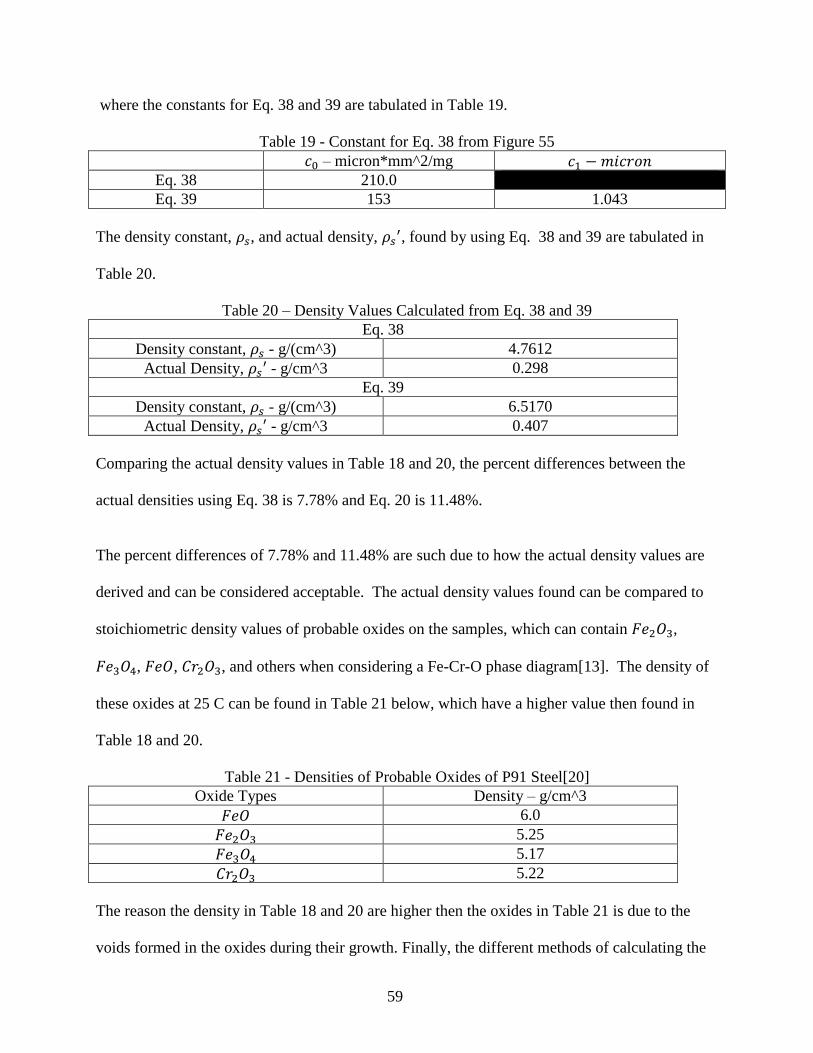
where the constants for Eq. 38 and 39 are tabulated in Table 19.
Table 19 - Constant for Eq. 38 from Figure 55
𝑐0 – micron*mm^2/mg 𝑐1 − 𝑚𝑖𝑐𝑟𝑜𝑛
Eq. 38 210.0
Eq. 39 153 1.043
The density constant, 𝜌𝑠, and actual density, 𝜌𝑠′, found by using Eq. 38 and 39 are tabulated in
Table 20.
Table 20 – Density Values Calculated from Eq. 38 and 39
Eq. 38
Density constant, 𝜌𝑠 - g/(cm^3) 4.7612
Actual Density, 𝜌𝑠′ - g/cm^3 0.298
Eq. 39
Density constant, 𝜌𝑠 - g/(cm^3) 6.5170
Actual Density, 𝜌𝑠′ - g/cm^3 0.407
Comparing the actual density values in Table 18 and 20, the percent differences between the
actual densities using Eq. 38 is 7.78% and Eq. 20 is 11.48%.
The percent differences of 7.78% and 11.48% are such due to how the actual density values are
derived and can be considered acceptable. The actual density values found can be compared to
stoichiometric density values of probable oxides on the samples, which can contain 𝐹𝑒2𝑂3,
𝐹𝑒3𝑂4, 𝐹𝑒𝑂, 𝐶𝑟2𝑂3, and others when considering a Fe-Cr-O phase diagram[13]. The density of
these oxides at 25 C can be found in Table 21 below, which have a higher value then found in
Table 18 and 20.
Table 21 - Densities of Probable Oxides of P91 Steel[20]
Oxide Types Density – g/cm^3
𝐹𝑒𝑂 6.0
𝐹𝑒2𝑂3 5.25
𝐹𝑒3𝑂4 5.17
𝐶𝑟2𝑂3 5.22
The reason the density in Table 18 and 20 are higher then the oxides in Table 21 is due to the
voids formed in the oxides during their growth. Finally, the different methods of calculating the
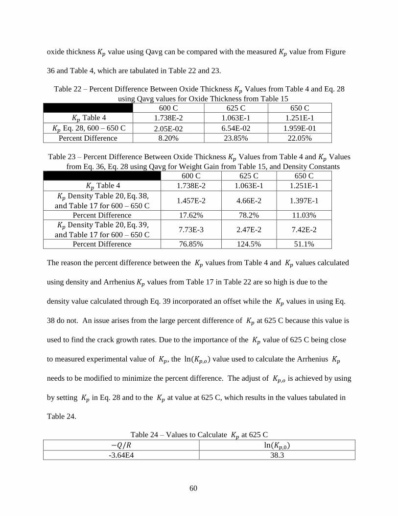
60
oxide thickness 𝐾𝑝 value using Qavg can be compared with the measured 𝐾𝑝 value from Figure
36 and Table 4, which are tabulated in Table 22 and 23.
Table 22 – Percent Difference Between Oxide Thickness 𝐾𝑝 Values from Table 4 and Eq. 28
using Qavg values for Oxide Thickness from Table 15
600 C 625 C 650 C
𝐾𝑝 Table 4 1.738E-2 1.063E-1 1.251E-1
𝐾𝑝 Eq. 28, 600 – 650 C 2.05E-02 6.54E-02 1.959E-01
Percent Difference 8.20% 23.85% 22.05%
Table 23 – Percent Difference Between Oxide Thickness 𝐾𝑝 Values from Table 4 and 𝐾𝑝 Values
from Eq. 36, Eq. 28 using Qavg for Weight Gain from Table 15, and Density Constants
600 C 625 C 650 C
𝐾𝑝 Table 4 1.738E-2 1.063E-1 1.251E-1
𝐾𝑝 Density Table 20, Eq. 38,
and Table 17 for 600 – 650 C 1.457E-2 4.66E-2 1.397E-1
Percent Difference 17.62% 78.2% 11.03%
𝐾𝑝 Density Table 20, Eq. 39,
and Table 17 for 600 – 650 C 7.73E-3 2.47E-2 7.42E-2
Percent Difference 76.85% 124.5% 51.1%
The reason the percent difference between the 𝐾𝑝 values from Table 4 and 𝐾𝑝 values calculated
using density and Arrhenius 𝐾𝑝 values from Table 17 in Table 22 are so high is due to the
density value calculated through Eq. 39 incorporated an offset while the 𝐾𝑝 values in using Eq.
38 do not. An issue arises from the large percent difference of 𝐾𝑝 at 625 C because this value is
used to find the crack growth rates. Due to the importance of the 𝐾𝑝 value of 625 C being close
to measured experimental value of 𝐾𝑝, the ln (𝐾𝑝,𝑜) value used to calculate the Arrhenius 𝐾𝑝
needs to be modified to minimize the percent difference. The adjust of 𝐾𝑝,𝑜 is achieved by using
by setting 𝐾𝑝 in Eq. 28 and to the 𝐾𝑝 at value at 625 C, which results in the values tabulated in
Table 24.
Table 24 – Values to Calculate 𝐾𝑝 at 625 C
−𝑄/𝑅 ln (𝐾𝑝,0)
-3.64E4 38.3
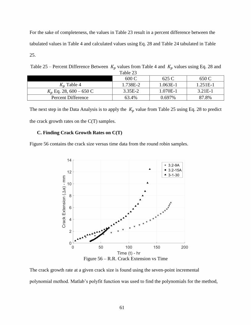
61
For the sake of completeness, the values in Table 23 result in a percent difference between the
tabulated values in Table 4 and calculated values using Eq. 28 and Table 24 tabulated in Table
25.
Table 25 – Percent Difference Between 𝐾𝑝 values from Table 4 and 𝐾𝑝 values using Eq. 28 and
Table 23
600 C 625 C 650 C
𝐾𝑝 Table 4 1.738E-2 1.063E-1 1.251E-1
𝐾𝑝 Eq. 28, 600 – 650 C 3.35E-2 1.070E-1 3.21E-1
Percent Difference 63.4% 0.697% 87.8%
The next step in the Data Analysis is to apply the 𝐾𝑝 value from Table 25 using Eq. 28 to predict
the crack growth rates on the C(T) samples.
C. Finding Crack Growth Rates on C(T)
Figure 56 contains the crack size versus time data from the round robin samples.
Figure 56 – R.R. Crack Extension vs Time
The crack growth rate at a given crack size is found using the seven-point incremental
polynomial method. Matlab’s polyfit function was used to find the polynomials for the method,
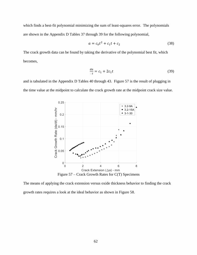
62
which finds a best-fit polynomial minimizing the sum of least-squares error. The polynomials
are shown in the Appendix D Tables 37 through 39 for the following polynomial,
𝑎 = 𝑐0𝑡2 + 𝑐1𝑡 + 𝑐2 (38)
The crack growth data can be found by taking the derivative of the polynomial best fit, which
becomes,
𝑑𝑎
𝑦𝑡= 𝑐1 + 2𝑐1𝑡 (39)
and is tabulated in the Appendix D Tables 40 through 43. Figure 57 is the result of plugging in
the time value at the midpoint to calculate the crack growth rate at the midpoint crack size value.
Figure 57 – Crack Growth Rates for C(T) Specimens
The means of applying the crack extension versus oxide thickness behavior to finding the crack
growth rates requires a look at the ideal behavior as shown in Figure 58.
63
Figure 58 - ideal crack extension versus oxide thickness
Figure 58 shows that at the start or opening of the crack the oxide thickness is at the maximum
value and then decreases when approaching the end. The crack extension versus oxide thickness
behavior can be converted into the crack growth rate versus time by starting with the following,
∆𝑎(𝑥) = 𝑓(𝑥) (40)
where 𝑓(𝑥) is the function modeling the behavior. Next, taking the derivative leads to,
𝑑(∆𝑎)
𝑑𝑥=
𝑑(𝑓(𝑥))
𝑑𝑥 (41)
which when multiplied by the derivative of oxide thickness over time,
𝑑(∆𝑎)
𝑑𝑡=
𝑑𝑥
𝑑𝑡
𝑑(𝑓(𝑥))
𝑑𝑥 (42)
However an issue arises with the behavior in Figure 58 and Eq. 42 is the negative value
generated when finding the derivative, which does not match the crack growth rate behavior in
Figure 57. The solution to this problem is the fact there is a difference in oxidation or exposure
time and time the crack end point was at the crack extension value. The modeling of this time
difference is,
64
𝑡′ = 𝑡𝑓 − 𝑡 (43)
where 𝑡′ is the time value at the crack extension value, 𝑡𝑓 is the time value at the crack end point,
and 𝑡 is the oxidation or exposure time. The significant of Eq. 43 is being able to convert the
oxidation or exposure time into the same time units of the C(T) data. Eq. 42 is converted into,
𝑑(∆𝑎)
𝑑𝑡′=
𝑑𝑥
𝑑𝑡′
𝑑(𝑓(𝑥))
𝑑𝑥 (44)
where the derivative of the oxide thickness over time is modeled through Eq. 9 and 43. Staring
with Eq. 9 and 43 the oxide thickness converted to time at the crack extension value is,
𝑥 = √𝑘𝑝(𝑡𝑓 − 𝑡′) (45)
and the derivative with respect to time is,
𝑑𝑥
𝑑𝑡′= −
𝑘𝑝
2𝑥 (46)
which the negative sign value takes care of the negative slope of Figure 58. Combing Eq. 44 and
46 leads to the conversion of crack extension versus oxide thickness behavior to crack growth
with,
𝑑(∆𝑎)
𝑑𝑡′= −
𝑘𝑝
2𝑥
𝑑(𝑓(𝑥))
𝑑𝑥 (47)
or,
𝑑(∆𝑎)
𝑑𝑡′= −
𝑘𝑝
2𝑥𝑑𝑥
𝑑(𝑓(𝑥))
(48)
where the benefit of Eq. 48 is only the oxide thickness versus crack extension behavior is needed
to find the crack growth rates. The actual crack extension versus oxide thickness behavior is
shown in Figure 59.
65
Figure 59 – Crack Extension vs Oxide Thickness
Figure 59 shows that there is a far amount of scatter in the oxide thickness values collected,
which can be smoothed by using an averaging technique. The averaging technique can be shown
by taking the original crack extension and oxide thickness data,
∆𝑎 = [∆𝑎𝑖, ∆𝑎𝑖+1, … , ∆𝑎𝑛−1, ∆𝑎𝑛] (49)
𝑥 = [𝑥𝑖, 𝑥𝑖+1, … , 𝑥𝑛−1, 𝑥𝑛] (50)
and apply the following,
𝑥𝑎𝑣𝑔,𝑗 =𝑥𝑖+𝑥𝑖+1+𝑥𝑖+2
3 (51)
The corresponding crack extension value to 𝑥𝑎𝑣𝑔,𝑗 is,
∆𝑎𝑎𝑣𝑔,𝑗 = ∆𝑎𝑖+1 (52)
which leads to the crack extension and oxide thickness values to be,
∆𝑎𝑎𝑣𝑔 = [∆𝑎𝑎𝑣𝑔,𝑗, ∆𝑎𝑎𝑣𝑔,𝑗+1, … , ∆𝑎𝑎𝑣𝑔,𝑚−1, ∆𝑎𝑎𝑣𝑔,𝑚] (53)
𝑥𝑎𝑣𝑔 = [𝑥𝑎𝑣𝑔,𝑗, 𝑥𝑎𝑣𝑔,𝑗+1, … , 𝑥𝑎𝑣𝑦,𝑚−1, 𝑥𝑎𝑣𝑔,𝑚] (54)
66
where 𝑗 = 𝑖 − 1 and 𝑚 = 𝑛 − 2. Eq. 53 and 54 expressed in terms of the raw data in Eq. 49 and
50 are,
∆𝑎𝑎𝑣𝑔 = [∆𝑎𝑖+1, ∆𝑎𝑖+2, … , ∆𝑎𝑛−2, ∆𝑎𝑛−1] (55)
𝑥𝑎𝑣𝑔 = [𝑥𝑖+𝑥𝑖+1+𝑥𝑖+2
3, … ,
𝑥𝑛−2+𝑥𝑛−1+𝑥𝑛
3] (56)
The downside to this method comes from the lose of two data points at the beginning and end,
but the results applied to the crack extension versus oxide thickness behavior from Figure 59 as
shown in Figure 60 show closer agreement to the ideal behavior seen in Figure 58.
(a)
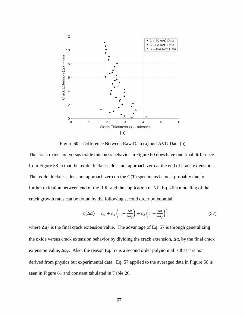
67
(b)
Figure 60 – Difference Between Raw Data (a) and AVG Data (b)
The crack extension versus oxide thickness behavior in Figure 60 does have one final difference
from Figure 58 in that the oxide thickness does not approach zero at the end of crack extension.
The oxide thickness does not approach zero on the C(T) specimens is most probably due to
further oxidation between end of the R.R. and the application of Ni. Eq. 48’s modeling of the
crack growth rates can be found by the following second order polynomial,
𝑥(∆𝑎) = 𝑐0 + 𝑐1 (1 −∆𝑎
∆𝑎𝑓) + 𝑐2 (1 −
∆𝑎
∆𝑎𝑓)
2
(57)
where ∆𝑎𝑓 is the final crack extension value. The advantage of Eq. 57 is through generalizing
the oxide versus crack extension behavior by dividing the crack extension, ∆𝑎, by the final crack
extension value, ∆𝑎𝑓. Also, the reason Eq. 57 is a second order polynomial is that it is not
derived from physics but experimental data. Eq. 57 applied to the averaged data in Figure 60 is
seen in Figure 61 and constant tabulated in Table 26.
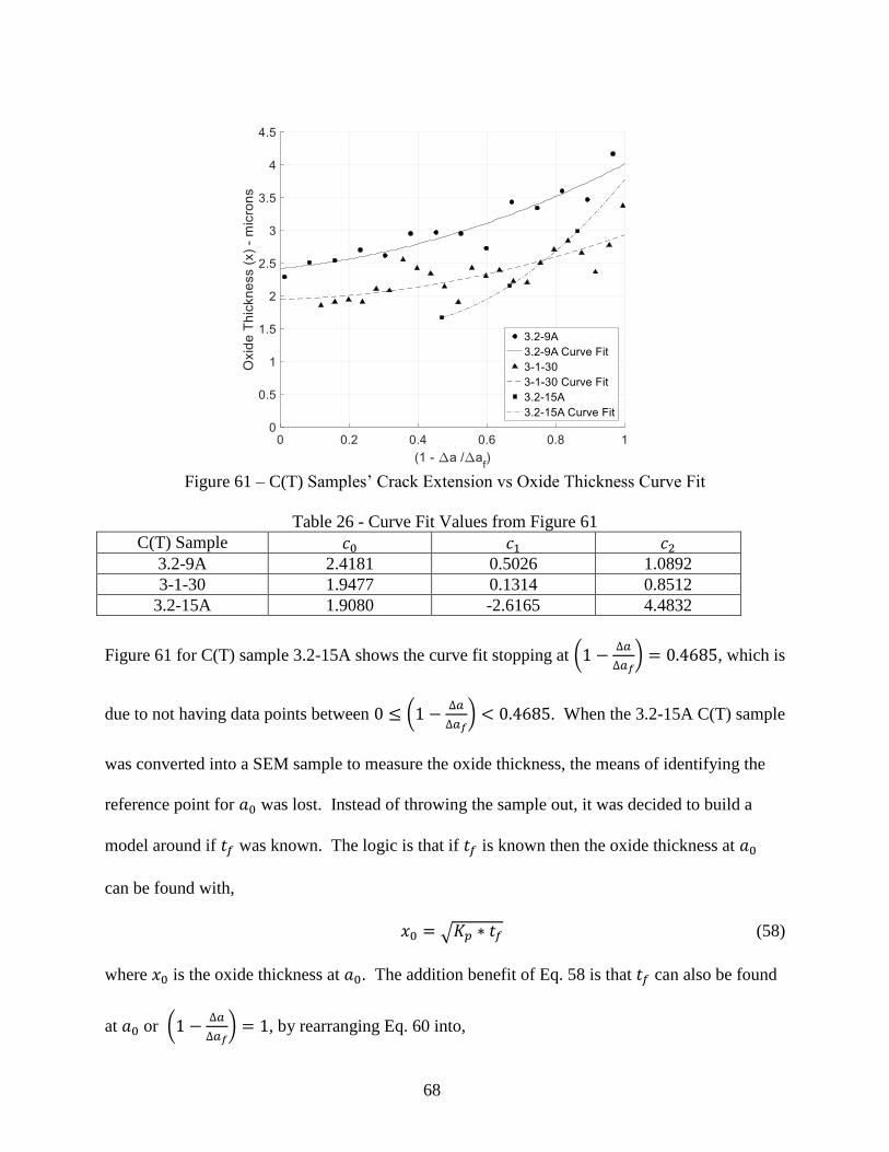
68
Figure 61 – C(T) Samples’ Crack Extension vs Oxide Thickness Curve Fit
Table 26 - Curve Fit Values from Figure 61
C(T) Sample 𝑐0 𝑐1 𝑐2
3.2-9A 2.4181 0.5026 1.0892
3-1-30 1.9477 0.1314 0.8512
3.2-15A 1.9080 -2.6165 4.4832
Figure 61 for C(T) sample 3.2-15A shows the curve fit stopping at (1 −∆𝑎
∆𝑎𝑓) = 0.4685, which is
due to not having data points between 0 ≤ (1 −∆𝑎
∆𝑎𝑓) < 0.4685. When the 3.2-15A C(T) sample
was converted into a SEM sample to measure the oxide thickness, the means of identifying the
reference point for 𝑎0 was lost. Instead of throwing the sample out, it was decided to build a
model around if 𝑡𝑓 was known. The logic is that if 𝑡𝑓 is known then the oxide thickness at 𝑎0
can be found with,
𝑥0 = √𝐾𝑝 ∗ 𝑡𝑓 (58)
where 𝑥0 is the oxide thickness at 𝑎0. The addition benefit of Eq. 58 is that 𝑡𝑓 can also be found
at 𝑎0 or (1 −∆𝑎
∆𝑎𝑓) = 1, by rearranging Eq. 60 into,
69
𝑡𝑓 =𝑥0
2
𝐾𝑝 (59)
Using the values of Table 26 it is easy to find the value for 𝑥0, since at 𝑎0 ∆𝑎=0 and therefore 𝑥0
= 𝑐0 + 𝑐1 + 𝑐2 for the C(T). The relative error between the 𝑡𝑓 from the C(T) data and 𝑡𝑓
predicted from Eq. 57 and 59 using averaged or raw data is tabulated in Table 27.
Table 27 – Percent Difference between Measured 𝑡𝑓 and Predicted 𝑡𝑓
C(T) Sample 3-1-30 3.2-9A 3.2-15A
C(T) 𝑡𝑓 - hr 137.4 175.1 63.7
Eq. 59 using Eq. 57 and
AVG Data - hr
80.2 150.3 133.2
Percent Difference 53.5% 15.25% 70.6%
Eq. 59 using Eq. 57 and
Raw Data - hr
79.2 153.9 36.5
Percent Difference 53.8% 12.86% 54.4%
The decision to use the averaged or raw oxide thickness data depends only on 3-1-30 and 3.2-9A
due to 3.2-15A being selected based on 𝑡𝑓 and data points collected. Since there is not a large
difference between using the raw and averaged oxide thickness data, the recommendation is to
use the averaged oxide thickness data.
In order to show the validity of using the oxide thickness to predict the crack growth rates, the
correlation between the crack growth rates predicted by the oxide and values measured by the
C(T) data is found. The correlation between using Eq. 48 and the crack growth rates from Figure
57 is shown in Figure 62.
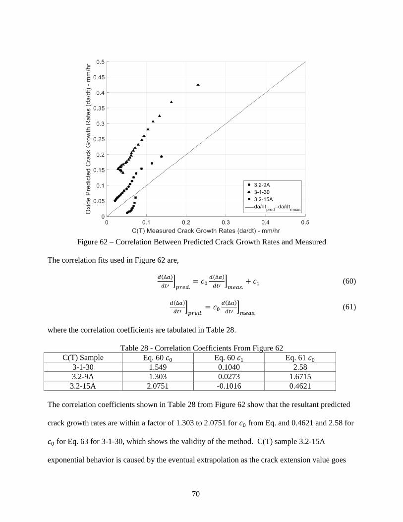
70
Figure 62 – Correlation Between Predicted Crack Growth Rates and Measured
The correlation fits used in Figure 62 are,
𝑑(∆𝑎)
𝑑𝑡′]
𝑝𝑟𝑒𝑑.= 𝑐0
𝑑(∆𝑎)
𝑑𝑡′]
𝑚𝑒𝑎𝑠.+ 𝑐1 (60)
𝑑(∆𝑎)
𝑑𝑡′]
𝑝𝑟𝑒𝑑.= 𝑐0
𝑑(∆𝑎)
𝑑𝑡′]
𝑚𝑒𝑎𝑠. (61)
where the correlation coefficients are tabulated in Table 28.
Table 28 - Correlation Coefficients From Figure 62
C(T) Sample Eq. 60 𝑐0 Eq. 60 𝑐1 Eq. 61 𝑐0
3-1-30 1.549 0.1040 2.58
3.2-9A 1.303 0.0273 1.6715
3.2-15A 2.0751 -0.1016 0.4621
The correlation coefficients shown in Table 28 from Figure 62 show that the resultant predicted
crack growth rates are within a factor of 1.303 to 2.0751 for 𝑐0 from Eq. and 0.4621 and 2.58 for
𝑐0 for Eq. 63 for 3-1-30, which shows the validity of the method. C(T) sample 3.2-15A
exponential behavior is caused by the eventual extrapolation as the crack extension value goes
71
beyond (1 −∆𝑎
∆𝑎𝑓) = 0.4685, which again is due to only having oxide thickness data up to
(1 −∆𝑎
∆𝑎𝑓) = 0.4685. The predicted versus actual crack growth values are left out of Figure 62
due to the predicted crack growth values become negative as ∆𝑎 approaches ∆𝑎𝑓. The negative
predicted values are not surprising due to trying to extrapolate values from a nonphysic but
experimentally derived model. Therefore the recommendation is to make sure you have
complete oxidation versus crack extension behavior for the sample. Figure 62 also shows a
discontinuity between the last three crack growth values for C(T) samples 3.2-9A and 3-1-30,
which is due to the sample entering into the third stage of creep crack growth. There are three
possible reasons this discontinuity has arisen,
1. The model needs to be altered to account for the third stage of creep crack growth.
2. The resulting oxide thickness measurements during the third state of creep crack growth
are hard to detect due to being near 𝑎𝑓 or more measurements are needed as ∆𝑎 increases.
3. The average smoothing technique masks the oxide thickness difference as ∆𝑎 increases.
To better illustrate the discontinuities between the predicted and measured crack growth rates,
the predicted and measured crack growth rates are plotted in Figure 63 versus crack extension.
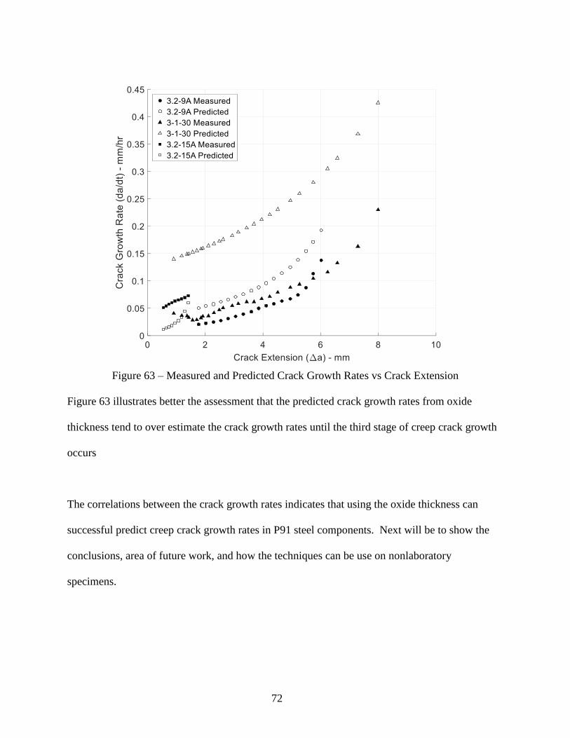
72
Figure 63 – Measured and Predicted Crack Growth Rates vs Crack Extension
Figure 63 illustrates better the assessment that the predicted crack growth rates from oxide
thickness tend to over estimate the crack growth rates until the third stage of creep crack growth
occurs
The correlations between the crack growth rates indicates that using the oxide thickness can
successful predict creep crack growth rates in P91 steel components. Next will be to show the
conclusions, area of future work, and how the techniques can be use on nonlaboratory
specimens.
73
VI. Conclusions and Future Work
A. Conclusion
Through the use of a simple parabolic model of oxidation kinetics, the ability to predict the crack
growth rates of P91 Steel components within a factor of 2.58 has been achieved. The
methodology involved in finding these results are,
1. Measure the oxide thickness of test samples to find the parabolic rate constant.
2. Measure the oxide thickness versus crack extension response of the P91 steel component.
3. Apply the 2nd degree polynomial, Eq. 57, to the oxide thickness versus crack extension
response.
4. Use the parabolic rate constant and Eq. 57 to predict the crack growth rates using Eq. 47.
B. Future Work
Next, are the future works that are necessary to further validate this technique. The first major
necessity of the techniques created through this research is to apply it to other materials.
Another major caveat of applying this technique to a new material is if the oxidation kinetics
does not match a parabolic model then Eq. 44 will need to be the starting point with the new
oxide kinetics instead of Eq. 48. Another area of future work would be the application using Eq.
60 to predict the age of the crack. A plastic replica can be used to in real world applications to
find the age of the crack, but finding an expectable value at which intervention is recommended
based off crack age and component thickness is necessary. One final suggestion would be to use
the type of oxides found on the P91 steel to predict the temperature the metal is at.
C. Improvements
Some improvements of the techniques would first be to change the Ni application portion of the
sample preparation for SEM. Validation is necessary of course, but the Ni application stage
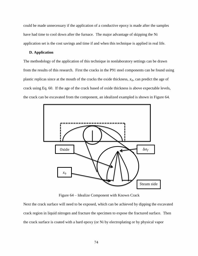
74
could be made unnecessary if the application of a conductive epoxy is made after the samples
have had time to cool down after the furnace. The major advantage of skipping the Ni
application set is the cost savings and time if and when this technique is applied in real life.
D. Application
The methodology of the application of this technique in nonlaboratory settings can be drawn
from the results of this research. First the cracks in the P91 steel components can be found using
plastic replicas since at the mouth of the cracks the oxide thickness, 𝑥0, can predict the age of
crack using Eq. 60. If the age of the crack based of oxide thickness is above expectable levels,
the crack can be excavated from the component, an idealized exampled is shown in Figure 64.
Figure 64 – Idealize Component with Known Crack
Next the crack surface will need to be exposed, which can be achieved by dipping the excavated
crack region in liquid nitrogen and fracture the specimen to expose the fractured surface. Then
the crack surface is coated with a hard epoxy (or Ni by electroplating or by physical vapor
𝑥0
Oxide ∆𝑎𝑓
Steam side
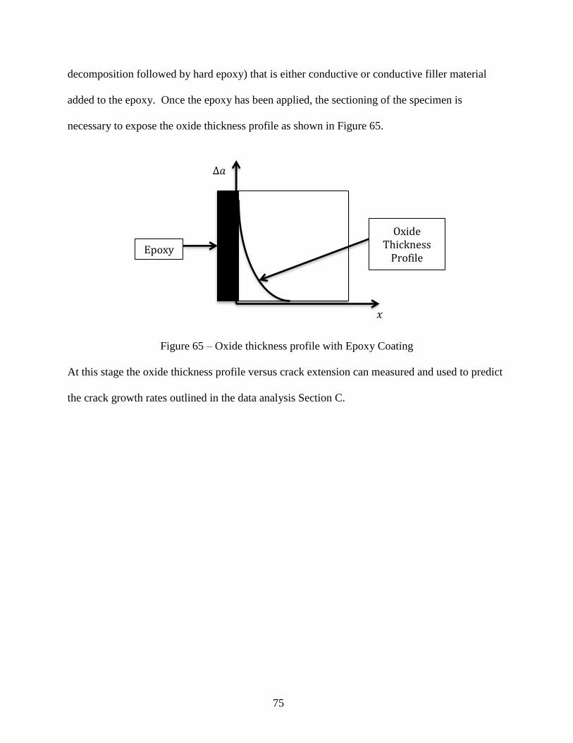
75
decomposition followed by hard epoxy) that is either conductive or conductive filler material
added to the epoxy. Once the epoxy has been applied, the sectioning of the specimen is
necessary to expose the oxide thickness profile as shown in Figure 65.
Figure 65 – Oxide thickness profile with Epoxy Coating
At this stage the oxide thickness profile versus crack extension can measured and used to predict
the crack growth rates outlined in the data analysis Section C.
Epoxy
Oxide Thickness
Profile
∆𝑎
𝑥

76
VII. References
1. A.Saxena, P.K. Liaw, and W.A. Logsdon, "Residual Life Prediction and Retirement for Cause
Criteria for SSTG Upper Casings, Part II: Fracture Mechanics Analysis, Engineering Fracture
Mechanics, vol. 25, 1986, pp. 289-303.
2. A. Saxena, Nonlinear Fracture Mechanics for Engineers, CRC Press, 199
3. A. Saxena editor, Comprehensive Structural Integrity, Volume 5-Creep, 2003
4. K.B. Yoon and A. Saxena, "An Interpretation of ∆J for Cyclically Unsaturated Materials,"
International Journal of Fracture, July 1991.
5. K.B. Yoon, A. Saxena and P.K. Liaw, "Characterization of Creep-Fatigue Crack Growth
Behavior Under Trapezoidal Waveshape Using Ct - Parameter," International Journal of
Fracture, Vol. 59, 1993, pp. 95-114.
6. K.B. Yoon, A. Saxena and D.L. McDowell, "Effect of Cyclic Overload on the Crack Growth
Behavior during Hold Period at Elevated Temperature", International Journal of Fracture, Vol.
59, 1993, pp. 199-211.
7. A. aSaxena, V. Kalyanasundaram and S.B. Narasimhachary, Prognostics for High Temperature
Component Reliability”, Invited Plenary Lecture, Thirteenth International Conference on
Fracture, ICF13, Beijing, China, June 16-21, 2013.
8. ASTM Standard E 2714-13: Standard Test Method for Creep-Fatigue Testing, ASTM Book of
Standards, ASTM International, W. Consohohocken, PA, 19428, 2013.
9. ASTM E2760-10: Standard Test Method for Creep-Fatigue Crack Growth Testing, ASTM Book
of Standards, ASTM International, W. Consohohocken, PA, 19428, 2010.
10. L.W. Pinder, “Oxide Characterization for Service Failure Investigations”, Corrosion Science,
Vol. 21, No. 11, pp. 749 – 763, 1981.
11. N. Birks, G. H. Meier and F. S. Pettit, Introduction to High Temperature Oxidation, New York:
Cambridge University Press, 2006.
12. Paul G. Shewmon, Diffusion in Solids, McGraw-Hill Book Company, Inc., 1963.
13. D. Young, High Temperature Oxidation and Corrosion of Metals, Oxford: Elsevier, 2008,.
14. T. Olszewski, “Oxidation Mechanisms of Materials for Heat Exchanging Components in
𝐶02/𝐻2𝑂-containing Gases Relevant to Oxy-fuel Environments”, Dissertation, RWTH Aachen
University, 2012.
77
15. P. Mathiazhagan and A. S. Khanna, “High Temperature Oxidation Behavior of P91, P92 and
E911 Alloy Steels in Dry and Wet Atmospheres,” High Temperature Material Process, Vol. 30,
2011, pp. 43 – 50.
16. ASTM Standard A335/A335M, 2011, “Standard Specification for Seamless Ferritic Alloy-Steel
Pipe for High-Temperature Service,” ASTM International, West Conshokocken, PA, 2011, DOI:
10.1520/A0355_A0355M-11, www.astm.org.
17. Ashok Saxena, V. Kalyanasundaram and Stuart R. Holdsworth, “Final Report on Round-robin
Conducted in Support of Standard Test Method for Creep-fatigue Testing”, EPRI Report
3002001719, Electric Power Research Institute, 3420 Hillview Ave., Palo Alto, CA, 94303, July
2013.
18. ASTM Standard E 3-11: Standard Guide for Preparation of Metallographic Specimens, ASTM
Book of Standards, ASTM International, W. Consohohocken, PA, 19428, 2011.
19. J. Raja and T. V. Vorburger, Surface Finish Metrology Tutorial, National Institute of Standards
and Testing, June 1990.
20. W. M. Haynes, David R. Lide and Thomas J. Bruno, CRC Handbook of Chemistry and Physics
97th Edition, CRC Press, Boca Raton, FL, 2017.
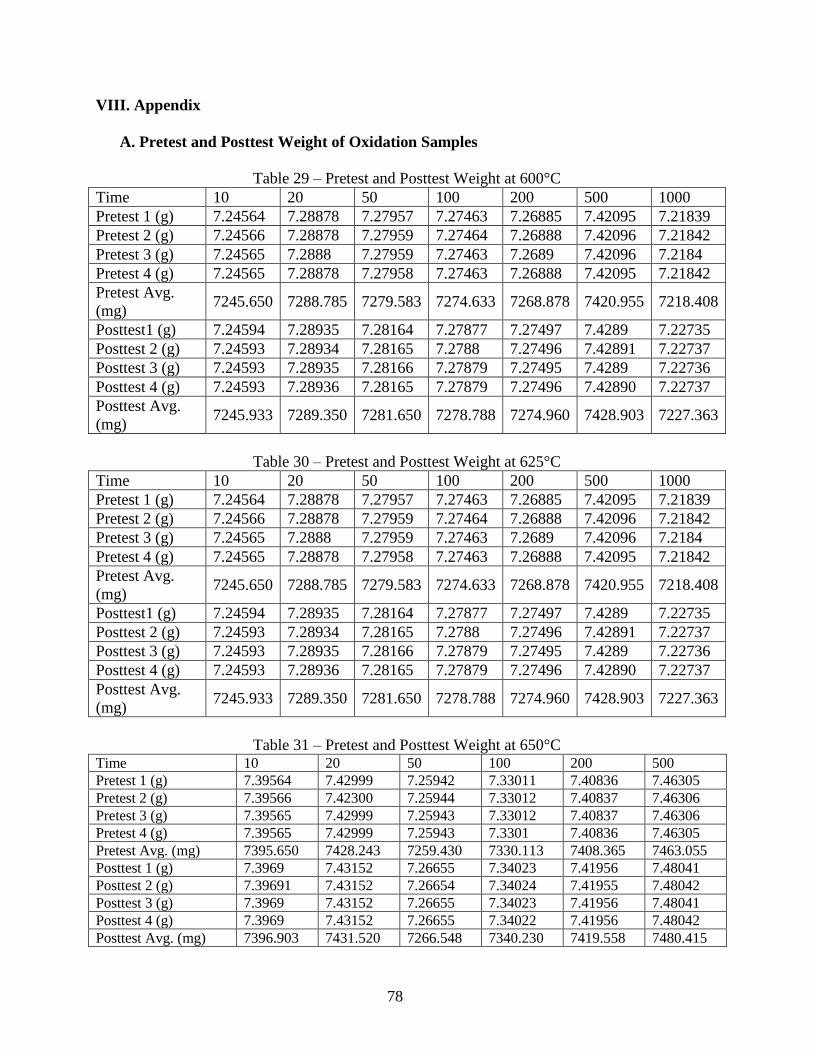
78
VIII. Appendix
A. Pretest and Posttest Weight of Oxidation Samples
Table 29 – Pretest and Posttest Weight at 600°C
Time 10 20 50 100 200 500 1000
Pretest 1 (g) 7.24564 7.28878 7.27957 7.27463 7.26885 7.42095 7.21839
Pretest 2 (g) 7.24566 7.28878 7.27959 7.27464 7.26888 7.42096 7.21842
Pretest 3 (g) 7.24565 7.2888 7.27959 7.27463 7.2689 7.42096 7.2184
Pretest 4 (g) 7.24565 7.28878 7.27958 7.27463 7.26888 7.42095 7.21842
Pretest Avg.
(mg) 7245.650 7288.785 7279.583 7274.633 7268.878 7420.955 7218.408
Posttest1 (g) 7.24594 7.28935 7.28164 7.27877 7.27497 7.4289 7.22735
Posttest 2 (g) 7.24593 7.28934 7.28165 7.2788 7.27496 7.42891 7.22737
Posttest 3 (g) 7.24593 7.28935 7.28166 7.27879 7.27495 7.4289 7.22736
Posttest 4 (g) 7.24593 7.28936 7.28165 7.27879 7.27496 7.42890 7.22737
Posttest Avg.
(mg) 7245.933 7289.350 7281.650 7278.788 7274.960 7428.903 7227.363
Table 30 – Pretest and Posttest Weight at 625°C
Time 10 20 50 100 200 500 1000
Pretest 1 (g) 7.24564 7.28878 7.27957 7.27463 7.26885 7.42095 7.21839
Pretest 2 (g) 7.24566 7.28878 7.27959 7.27464 7.26888 7.42096 7.21842
Pretest 3 (g) 7.24565 7.2888 7.27959 7.27463 7.2689 7.42096 7.2184
Pretest 4 (g) 7.24565 7.28878 7.27958 7.27463 7.26888 7.42095 7.21842
Pretest Avg.
(mg) 7245.650 7288.785 7279.583 7274.633 7268.878 7420.955 7218.408
Posttest1 (g) 7.24594 7.28935 7.28164 7.27877 7.27497 7.4289 7.22735
Posttest 2 (g) 7.24593 7.28934 7.28165 7.2788 7.27496 7.42891 7.22737
Posttest 3 (g) 7.24593 7.28935 7.28166 7.27879 7.27495 7.4289 7.22736
Posttest 4 (g) 7.24593 7.28936 7.28165 7.27879 7.27496 7.42890 7.22737
Posttest Avg.
(mg) 7245.933 7289.350 7281.650 7278.788 7274.960 7428.903 7227.363
Table 31 – Pretest and Posttest Weight at 650°C Time 10 20 50 100 200 500
Pretest 1 (g) 7.39564 7.42999 7.25942 7.33011 7.40836 7.46305
Pretest 2 (g) 7.39566 7.42300 7.25944 7.33012 7.40837 7.46306
Pretest 3 (g) 7.39565 7.42999 7.25943 7.33012 7.40837 7.46306
Pretest 4 (g) 7.39565 7.42999 7.25943 7.3301 7.40836 7.46305
Pretest Avg. (mg) 7395.650 7428.243 7259.430 7330.113 7408.365 7463.055
Posttest 1 (g) 7.3969 7.43152 7.26655 7.34023 7.41956 7.48041
Posttest 2 (g) 7.39691 7.43152 7.26654 7.34024 7.41955 7.48042
Posttest 3 (g) 7.3969 7.43152 7.26655 7.34023 7.41956 7.48041
Posttest 4 (g) 7.3969 7.43152 7.26655 7.34022 7.41956 7.48042
Posttest Avg. (mg) 7396.903 7431.520 7266.548 7340.230 7419.558 7480.415
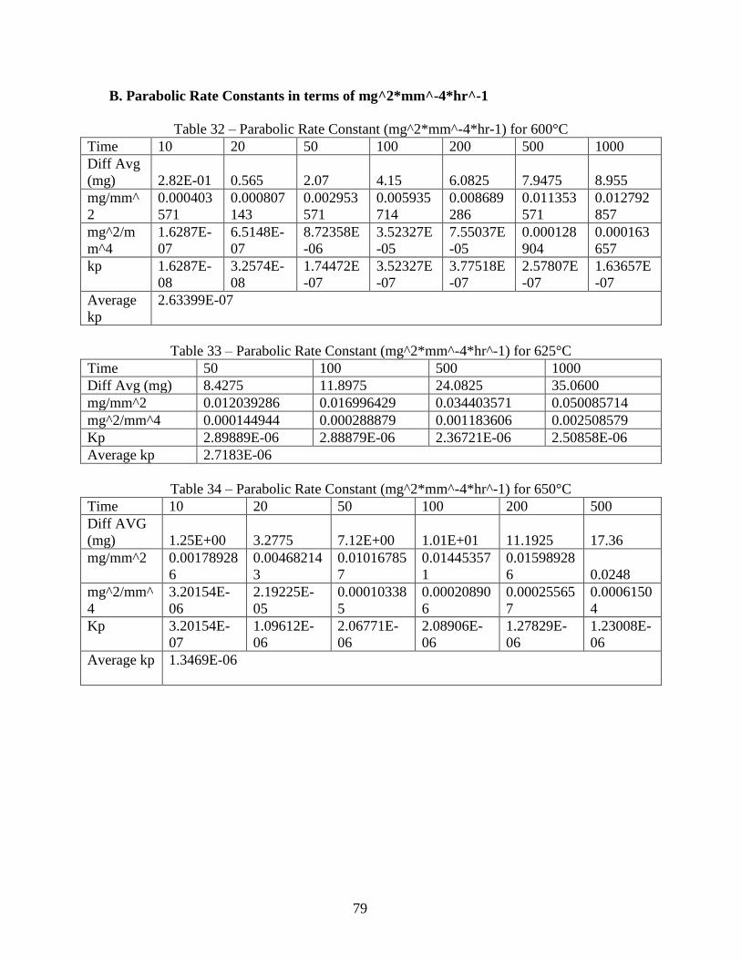
79
B. Parabolic Rate Constants in terms of mg^2*mm^-4*hr^-1
Table 32 – Parabolic Rate Constant (mg^2*mm^-4*hr-1) for 600°C
Time 10 20 50 100 200 500 1000
Diff Avg
(mg) 2.82E-01 0.565 2.07 4.15 6.0825 7.9475 8.955
mg/mm^
2
0.000403
571
0.000807
143
0.002953
571
0.005935
714
0.008689
286
0.011353
571
0.012792
857
mg^2/m
m^4
1.6287E-
07
6.5148E-
07
8.72358E
-06
3.52327E
-05
7.55037E
-05
0.000128
904
0.000163
657
kp 1.6287E-
08
3.2574E-
08
1.74472E
-07
3.52327E
-07
3.77518E
-07
2.57807E
-07
1.63657E
-07
Average
kp
2.63399E-07
Table 33 – Parabolic Rate Constant (mg^2*mm^-4*hr^-1) for 625°C
Time 50 100 500 1000
Diff Avg (mg) 8.4275 11.8975 24.0825 35.0600
mg/mm^2 0.012039286 0.016996429 0.034403571 0.050085714
mg^2/mm^4 0.000144944 0.000288879 0.001183606 0.002508579
Kp 2.89889E-06 2.88879E-06 2.36721E-06 2.50858E-06
Average kp 2.7183E-06
Table 34 – Parabolic Rate Constant (mg^2*mm^-4*hr^-1) for 650°C
Time 10 20 50 100 200 500
Diff AVG
(mg) 1.25E+00 3.2775 7.12E+00 1.01E+01 11.1925 17.36
mg/mm^2 0.00178928
6
0.00468214
3
0.01016785
7
0.01445357
1
0.01598928
6 0.0248
mg^2/mm^
4
3.20154E-
06
2.19225E-
05
0.00010338
5
0.00020890
6
0.00025565
7
0.0006150
4
Kp 3.20154E-
07
1.09612E-
06
2.06771E-
06
2.08906E-
06
1.27829E-
06
1.23008E-
06
Average kp 1.3469E-06
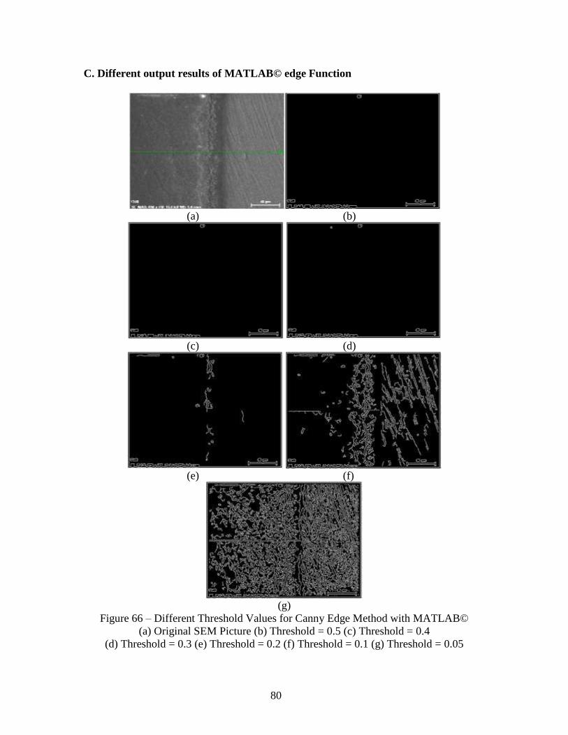
80
C. Different output results of MATLAB© edge Function
(a) (b)
(c) (d)
(e) (f)
(g)
Figure 66 – Different Threshold Values for Canny Edge Method with MATLAB©
(a) Original SEM Picture (b) Threshold = 0.5 (c) Threshold = 0.4
(d) Threshold = 0.3 (e) Threshold = 0.2 (f) Threshold = 0.1 (g) Threshold = 0.05
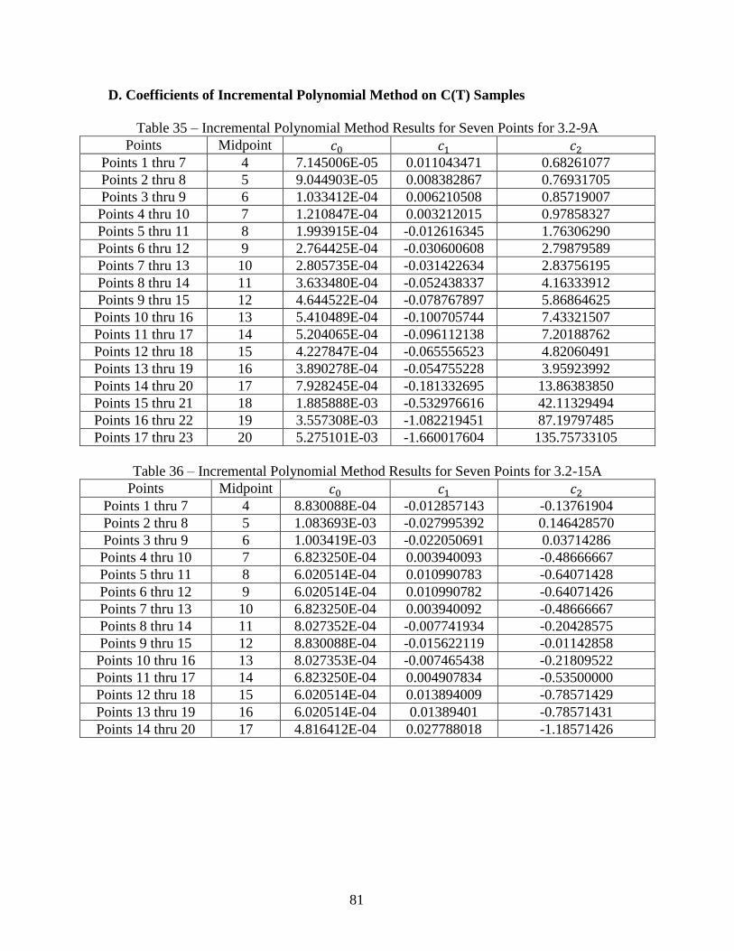
81
D. Coefficients of Incremental Polynomial Method on C(T) Samples
Table 35 – Incremental Polynomial Method Results for Seven Points for 3.2-9A
Points Midpoint 𝑐0 𝑐1 𝑐2
Points 1 thru 7 4 7.145006E-05 0.011043471 0.68261077
Points 2 thru 8 5 9.044903E-05 0.008382867 0.76931705
Points 3 thru 9 6 1.033412E-04 0.006210508 0.85719007
Points 4 thru 10 7 1.210847E-04 0.003212015 0.97858327
Points 5 thru 11 8 1.993915E-04 -0.012616345 1.76306290
Points 6 thru 12 9 2.764425E-04 -0.030600608 2.79879589
Points 7 thru 13 10 2.805735E-04 -0.031422634 2.83756195
Points 8 thru 14 11 3.633480E-04 -0.052438337 4.16333912
Points 9 thru 15 12 4.644522E-04 -0.078767897 5.86864625
Points 10 thru 16 13 5.410489E-04 -0.100705744 7.43321507
Points 11 thru 17 14 5.204065E-04 -0.096112138 7.20188762
Points 12 thru 18 15 4.227847E-04 -0.065556523 4.82060491
Points 13 thru 19 16 3.890278E-04 -0.054755228 3.95923992
Points 14 thru 20 17 7.928245E-04 -0.181332695 13.86383850
Points 15 thru 21 18 1.885888E-03 -0.532976616 42.11329494
Points 16 thru 22 19 3.557308E-03 -1.082219451 87.19797485
Points 17 thru 23 20 5.275101E-03 -1.660017604 135.75733105
Table 36 – Incremental Polynomial Method Results for Seven Points for 3.2-15A
Points Midpoint 𝑐0 𝑐1 𝑐2
Points 1 thru 7 4 8.830088E-04 -0.012857143 -0.13761904
Points 2 thru 8 5 1.083693E-03 -0.027995392 0.146428570
Points 3 thru 9 6 1.003419E-03 -0.022050691 0.03714286
Points 4 thru 10 7 6.823250E-04 0.003940093 -0.48666667
Points 5 thru 11 8 6.020514E-04 0.010990783 -0.64071428
Points 6 thru 12 9 6.020514E-04 0.010990782 -0.64071426
Points 7 thru 13 10 6.823250E-04 0.003940092 -0.48666667
Points 8 thru 14 11 8.027352E-04 -0.007741934 -0.20428575
Points 9 thru 15 12 8.830088E-04 -0.015622119 -0.01142858
Points 10 thru 16 13 8.027353E-04 -0.007465438 -0.21809522
Points 11 thru 17 14 6.823250E-04 0.004907834 -0.53500000
Points 12 thru 18 15 6.020514E-04 0.013894009 -0.78571429
Points 13 thru 19 16 6.020514E-04 0.01389401 -0.78571431
Points 14 thru 20 17 4.816412E-04 0.027788018 -1.18571426
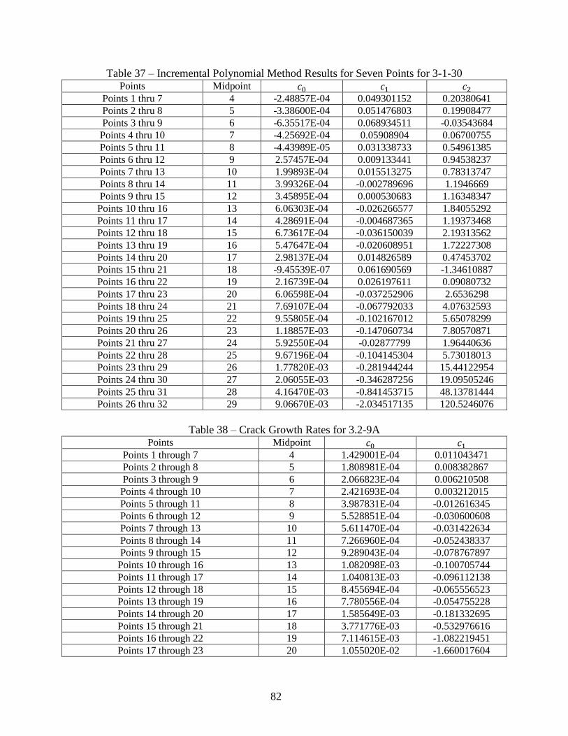
82
Table 37 – Incremental Polynomial Method Results for Seven Points for 3-1-30 Points Midpoint 𝑐0 𝑐1 𝑐2
Points 1 thru 7 4 -2.48857E-04 0.049301152 0.20380641
Points 2 thru 8 5 -3.38600E-04 0.051476803 0.19908477
Points 3 thru 9 6 -6.35517E-04 0.068934511 -0.03543684
Points 4 thru 10 7 -4.25692E-04 0.05908904 0.06700755
Points 5 thru 11 8 -4.43989E-05 0.031338733 0.54961385
Points 6 thru 12 9 2.57457E-04 0.009133441 0.94538237
Points 7 thru 13 10 1.99893E-04 0.015513275 0.78313747
Points 8 thru 14 11 3.99326E-04 -0.002789696 1.1946669
Points 9 thru 15 12 3.45895E-04 0.000530683 1.16348347
Points 10 thru 16 13 6.06303E-04 -0.026266577 1.84055292
Points 11 thru 17 14 4.28691E-04 -0.004687365 1.19373468
Points 12 thru 18 15 6.73617E-04 -0.036150039 2.19313562
Points 13 thru 19 16 5.47647E-04 -0.020608951 1.72227308
Points 14 thru 20 17 2.98137E-04 0.014826589 0.47453702
Points 15 thru 21 18 -9.45539E-07 0.061690569 -1.34610887
Points 16 thru 22 19 2.16739E-04 0.026197611 0.09080732
Points 17 thru 23 20 6.06598E-04 -0.037252906 2.6536298
Points 18 thru 24 21 7.69107E-04 -0.067792033 4.07632593
Points 19 thru 25 22 9.55805E-04 -0.102167012 5.65078299
Points 20 thru 26 23 1.18857E-03 -0.147060734 7.80570871
Points 21 thru 27 24 5.92550E-04 -0.02877799 1.96440636
Points 22 thru 28 25 9.67196E-04 -0.104145304 5.73018013
Points 23 thru 29 26 1.77820E-03 -0.281944244 15.44122954
Points 24 thru 30 27 2.06055E-03 -0.346287256 19.09505246
Points 25 thru 31 28 4.16470E-03 -0.841453715 48.13781444
Points 26 thru 32 29 9.06670E-03 -2.034517135 120.5246076
Table 38 – Crack Growth Rates for 3.2-9A Points Midpoint 𝑐0 𝑐1
Points 1 through 7 4 1.429001E-04 0.011043471
Points 2 through 8 5 1.808981E-04 0.008382867
Points 3 through 9 6 2.066823E-04 0.006210508
Points 4 through 10 7 2.421693E-04 0.003212015
Points 5 through 11 8 3.987831E-04 -0.012616345
Points 6 through 12 9 5.528851E-04 -0.030600608
Points 7 through 13 10 5.611470E-04 -0.031422634
Points 8 through 14 11 7.266960E-04 -0.052438337
Points 9 through 15 12 9.289043E-04 -0.078767897
Points 10 through 16 13 1.082098E-03 -0.100705744
Points 11 through 17 14 1.040813E-03 -0.096112138
Points 12 through 18 15 8.455694E-04 -0.065556523
Points 13 through 19 16 7.780556E-04 -0.054755228
Points 14 through 20 17 1.585649E-03 -0.181332695
Points 15 through 21 18 3.771776E-03 -0.532976616
Points 16 through 22 19 7.114615E-03 -1.082219451
Points 17 through 23 20 1.055020E-02 -1.660017604
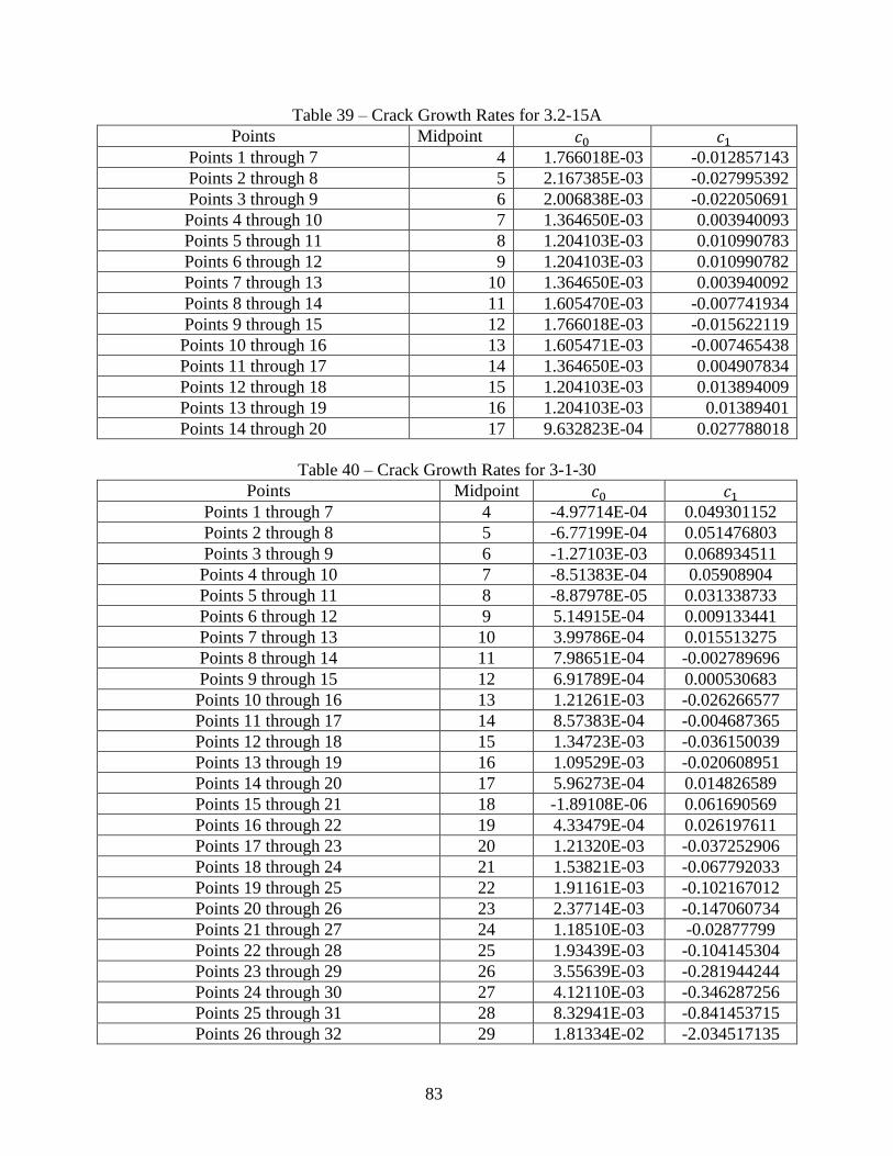
83
Table 39 – Crack Growth Rates for 3.2-15A
Points Midpoint 𝑐0 𝑐1
Points 1 through 7 4 1.766018E-03 -0.012857143
Points 2 through 8 5 2.167385E-03 -0.027995392
Points 3 through 9 6 2.006838E-03 -0.022050691
Points 4 through 10 7 1.364650E-03 0.003940093
Points 5 through 11 8 1.204103E-03 0.010990783
Points 6 through 12 9 1.204103E-03 0.010990782
Points 7 through 13 10 1.364650E-03 0.003940092
Points 8 through 14 11 1.605470E-03 -0.007741934
Points 9 through 15 12 1.766018E-03 -0.015622119
Points 10 through 16 13 1.605471E-03 -0.007465438
Points 11 through 17 14 1.364650E-03 0.004907834
Points 12 through 18 15 1.204103E-03 0.013894009
Points 13 through 19 16 1.204103E-03 0.01389401
Points 14 through 20 17 9.632823E-04 0.027788018
Table 40 – Crack Growth Rates for 3-1-30
Points Midpoint 𝑐0 𝑐1
Points 1 through 7 4 -4.97714E-04 0.049301152
Points 2 through 8 5 -6.77199E-04 0.051476803
Points 3 through 9 6 -1.27103E-03 0.068934511
Points 4 through 10 7 -8.51383E-04 0.05908904
Points 5 through 11 8 -8.87978E-05 0.031338733
Points 6 through 12 9 5.14915E-04 0.009133441
Points 7 through 13 10 3.99786E-04 0.015513275
Points 8 through 14 11 7.98651E-04 -0.002789696
Points 9 through 15 12 6.91789E-04 0.000530683
Points 10 through 16 13 1.21261E-03 -0.026266577
Points 11 through 17 14 8.57383E-04 -0.004687365
Points 12 through 18 15 1.34723E-03 -0.036150039
Points 13 through 19 16 1.09529E-03 -0.020608951
Points 14 through 20 17 5.96273E-04 0.014826589
Points 15 through 21 18 -1.89108E-06 0.061690569
Points 16 through 22 19 4.33479E-04 0.026197611
Points 17 through 23 20 1.21320E-03 -0.037252906
Points 18 through 24 21 1.53821E-03 -0.067792033
Points 19 through 25 22 1.91161E-03 -0.102167012
Points 20 through 26 23 2.37714E-03 -0.147060734
Points 21 through 27 24 1.18510E-03 -0.02877799
Points 22 through 28 25 1.93439E-03 -0.104145304
Points 23 through 29 26 3.55639E-03 -0.281944244
Points 24 through 30 27 4.12110E-03 -0.346287256
Points 25 through 31 28 8.32941E-03 -0.841453715
Points 26 through 32 29 1.81334E-02 -2.034517135
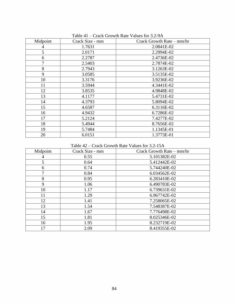
84
Table 41 – Crack Growth Rate Values for 3.2-9A
Midpoint Crack Size - mm Crack Growth Rate – mm/hr
4 1.7631 2.0841E-02
5 2.0171 2.2994E-02
6 2.2787 2.4736E-02
7 2.5403 2.7874E-02
8 2.7943 3.1263E-02
9 3.0585 3.5135E-02
10 3.3176 3.9236E-02
11 3.5944 4.3441E-02
12 3.8535 4.9848E-02
13 4.1177 5.4731E-02
14 4.3793 5.8094E-02
15 4.6587 6.3116E-02
16 4.9432 6.7286E-02
17 5.2124 7.4277E-02
18 5.4944 8.7656E-02
19 5.7484 1.1345E-01
20 6.0151 1.3773E-01
Table 42 – Crack Growth Rate Values for 3.2-15A
Midpoint Crack Size - mm Crack Growth Rate – mm/hr
4 0.55 5.101382E-02
5 0.64 5.412442E-02
6 0.74 5.744240E-02
7 0.84 6.034562E-02
8 0.95 6.283410E-02
9 1.06 6.490783E-02
10 1.17 6.739631E-02
11 1.29 6.967742E-02
12 1.41 7.258065E-02
13 1.54 7.548387E-02
14 1.67 7.776498E-02
15 1.81 8.025346E-02
16 1.95 8.232719E-02
17 2.09 8.419355E-02
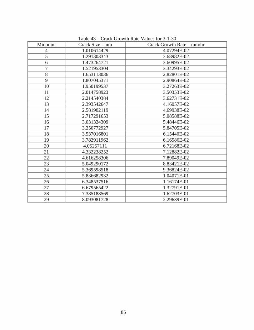
85
Table 43 – Crack Growth Rate Values for 3-1-30
Midpoint Crack Size - mm Crack Growth Rate – mm/hr
4 1.010614429 4.07294E-02
5 1.291303343 3.68982E-02
6 1.473264721 3.60995E-02
7 1.521953304 3.34293E-02
8 1.653113036 2.82801E-02
9 1.807045371 2.90864E-02
10 1.950199537 3.27263E-02
11 2.014758923 3.50353E-02
12 2.214540384 3.62731E-02
13 2.393542647 4.16057E-02
14 2.581902119 4.69938E-02
15 2.717291653 5.08588E-02
16 3.031324309 5.48446E-02
17 3.250772927 5.84705E-02
18 3.537016801 6.15440E-02
19 3.782911962 6.16586E-02
20 4.05257111 6.72168E-02
21 4.332238252 7.12882E-02
22 4.616258306 7.89049E-02
23 5.049290172 8.83421E-02
24 5.369598518 9.36824E-02
25 5.836682932 1.04071E-01
26 6.348537516 1.16174E-01
27 6.679565422 1.32791E-01
28 7.385188569 1.62703E-01
29 8.093081728 2.29639E-01
![by Shylesh Umapathyfresnostate.edu/.../Shylesh_Umapathy_Thesis_Report.pdfrequirements [3]. As transistors are getting smaller in size, there is reduction in the oxide thickness, gate](https://img.pdfslide.net/doc/110x75/5f95fe2f644ca52c186e630f/by-shylesh-requirements-3-as-transistors-are-getting-smaller-in-size-there-is.jpg)