Embed Size (px)
Citation preview
Feature selection for probabilistic load forecasting via sparsepenalized quantile regression
Yi WANG1 , Dahua GAN1, Ning ZHANG1, Le XIE2,
Chongqing KANG1
Abstract Probabilistic load forecasting (PLF) is able to
present the uncertainty information of the future loads. It is
the basis of stochastic power system planning and opera-
tion. Recent works on PLF mainly focus on how to develop
and combine forecasting models, while the feature selec-
tion issue has not been thoroughly investigated for PLF.
This paper fills the gap by proposing a feature selection
method for PLF via sparse L1-norm penalized quantile
regression. It can be viewed as an extension from point
forecasting-based feature selection to probabilistic fore-
casting-based feature selection. Since both the number of
training samples and the number of features to be selected
are very large, the feature selection process is casted as a
large-scale convex optimization problem. The alternating
direction method of multipliers is applied to solve the
problem in an efficient manner. We conduct case studies on
the open datasets of ten areas. Numerical results show that
the proposed feature selection method can improve the
performance of the probabilistic forecasting and outper-
forms traditional least absolute shrinkage and selection
operator method.
Keywords Probabilistic load forecasting, Feature
selection, Alternating direction method of multipliers
(ADMM), Quantile regression, L1-norm penalty
1 Introduction
The electrical load is affected by various factors such as
weather condition, distributed renewable integration,
demand response implementation, energy policy, emergent
events, etc. Traditional load forecasting only provides an
expected value of future load. In modern power system,
characterizing the uncertainties of future load will benefit
the reliability and economy of the whole system. More and
more probabilistic load forecasting (PLF) methods have
been proposed in recent years [1].
The whole process of load forecasting includes data
preprocessing, feature engineering, model establishment
and optimization, result analysis and visualization. Quan-
tile regression model is the most frequently used tool for
PFL. An embedding based quantile regression neural net-
work (QRNN) was proposed in [2] for PLF, where the
discrete variables such as day type, day of the week, and
hour of the day are modeled by the embedding matrix.
Another improved QRNN was presented in [3]. The net-
work involves Gaussian noise layer and dropout layer to
overcome the overfitting issue. A ‘‘separate-forecasting-
integrate’’ framework was proposed in [4] to forecast the
net load with high penetration of behind-the-meter
CrossCheck date: 18 April 2019
Received: 1 October 2018 / Accepted: 18 April 2019 / Published
online: 23 July 2019
� The Author(s) 2019
& Chongqing KANG
Yi WANG
Dahua GAN
Ning ZHANG
Le XIE
1 Department of Electrical Engineering, Tsinghua University,
Beijing, China
2 Department of Electrical and Computer Engineering, Texas
A&M University, Uvalde, TX, USA
123
J. Mod. Power Syst. Clean Energy (2019) 7(5):1200–1209
https://doi.org/10.1007/s40565-019-0552-3

photovoltaic (PV). The decomposed parts are forecasted by
QRNN, quantile random forest, or quantile gradient
boosting regression tree (QGBRT); while the dependencies
between load and PV uncertainties are modelled by copula
function and describe dependent convolution (DDC) [5].
Quantile, density, and interval are three main forms of
probabilistic forecasts. Kernel density estimation can make
a bridge between quantile forecast and density forecast.
The triangle kernel function was used in [6] to transform
the quantiles obtained by QRNN to density forecasts.
Since there have already existed various point load
forecasting methods, it is a good idea to transform the point
forecasts into probabilistic forecasts. A temperature sce-
nario generation approach was proposed in [7], where
various temperature scenarios were fed into the point
forecasting model to generate various point forecasts and
then the quantiles could be calculated based on the point
forecasts. A simple quantile regression averaging model
was established on multiple point forecasts generated by
sister forecasting models in [8]. A deep investigation of
point forecasting residual was conducted in [9]. Residual
simulation was implemented based on the normality
assumption to produce probabilistic forecasts. Instead of
focusing on specific PLF model, an ensemble approach was
proposed in [10] to combine the quantile probabilistic
forecasts of multiple models. The combining model was
formulated as a linear programing (LP) problem to mini-
mize the pinball loss of the final model.
PLF has also been applied for individual household in
addition to system-level load [11]. Conditional kernel
density estimation was used in [12] to model the condi-
tional distribution of residential load on different time
periods. In [13], the uncertainty within smart meter data
was forecasted by boosting additive quantile regression
model. Case studies show the superiority of the additive
model compared with the normality assumption-based
method. Gaussian process regression (GPR) was applied in
[14] for residential load forecasting, where different forms
of kernels were compared.
Most of the load forecasting literature focuses on the
establishment and optimization of the forecasting model;
while, very few research focuses on the preprocessing and
feature engineering phase, especially for PLF. Feature
selection, as an important part of the feature engineering,
tries to select the most useful or relevant features from the
original data to enhance the accuracy of load forecasts and
increase the interpretability of the forecasting model. When
the number of original features is too large, it can also be
used to reduce the solving complexity of the model. Most
of the research areas of feature selection are concentrated
in the traditional point forecasting, such as least absolute
shrinkage and selection operator (LASSO) method [15].
However, the feature selection in the field of probabilistic
forecasting has rarely been studied. To the best of our
knowledge, there is only one feature selection work for
PLF introduced in [16] by varying the number of lagged
hours and lagged days of the temperature. The proposed
global feature selection method is quite similar to the
exhaustive method. The method was tested on seven states
of the United States. The main idea is to evaluate the
performance of feature selection using pinball loss instead
of root mean square error (RMSE).
In this paper, we enrich the PLF feature selection liter-
ature by proposing a novel sparse penalized quantile
regression method. To tackle the challenges of large
computation burden and non-differentiable issue, alternat-
ing direction method of multipliers (ADMM) [17] is
applied to decompose the optimization problem. The
results show that the proposed feature selection method can
improve the performance of the original probabilistic
forecasting model compared with original model and
heuristic model.
The main contributions of this paper can be summarized
as follows:
1) Proposing a feature selection method for PLF by
introducing L1-norm sparse penalty into quantile
regression model.
2) Designing an ADMM algorithm to decouple the large-
scale optimization problem and boost the efficiency of
the model training process.
3) Validating the superiority of the proposed sparse
penalized quantile regression method by numerical
simulation based on the cases from the open
datasets.
The reminder of this paper is organized as follows:
Section 2 provides the dataset used and the regression
models for load forecasting; Section 3 introduces a
straightforward feature selection method which is used as
benchmark in the case studies; Section 4 introduces the
proposed feature selection method and the ADMM-based
training method; Section 5 presents the implementation
details of our proposed method; and Section 6 conducts the
case studies on the open datasets from Global Energy
Forecasting Competition in the year of 2012 (GEFCom
2012).
2 Data and model
2.1 Load dataset exploration
The load data used in this paper is the open dataset used
for GEFCom 2012 [18]. The dataset includes the 5 years of
hourly load data of 20 region power systems of North
Carolina from 2004 to 2008. The corresponding hourly
Feature selection for probabilistic load forecasting via sparse penalized quantile regression 1201
123
temperature data from 11 weather stations are also
provided.
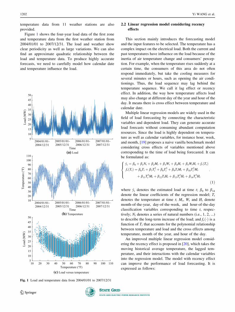
Figure 1 shows the four-year load data of the first zone
and temperature data from the first weather station from
2004/01/01 to 2007/12/31. The load and weather show
clear periodicity as well as large variations. We can also
find an approximate quadratic relationship between the
load and temperature data. To produce highly accurate
forecasts, we need to carefully model how calendar date
and temperature influence the load.
2.2 Linear regression model considering recency
effects
This section mainly introduces the forecasting model
and the input features to be selected. The temperature has a
complex impact on the electrical load. Both the current and
past temperatures have influence on the load because of the
inertia of air temperature change and consumers’ percep-
tion. For example, when the temperature rises suddenly at a
certain time, the consumers of this area do not often
respond immediately, but take the cooling measures for
several minutes or hours, such as opening the air condi-
tionings. Thus, the load sequence may lag behind the
temperature sequence. We call it lag effect or recency
effect. In addition, the way how temperature affects load
may also change at different day of the year and hour of the
day. It means there is cross effect between temperature and
calendar date.
Multiple linear regression models are widely used in the
field of load forecasting by connecting the characteristic
variables and dependent load. They can generate accurate
load forecasts without consuming abundant computation
resources. Since the load is highly dependent on tempera-
ture as well as calendar variables, for instance hour, week,
and month, [19] proposes a naive vanilla benchmark model
considering cross effects of variables mentioned above
corresponding to the time of load being forecasted. It can
be formulated as:
yt ¼ b0 þ b1Nt þ b2Mt þ b3Wt þ b4Ht þ b5WtHt þ frðTtÞfrðTtÞ ¼ b6Tt þ b7T
2t þ b8T
3t þ b9TtMt þ b10T
2t Mt
þ b11T3t Mt þ b12TtHt þ b13T
2t Ht þ b14T
3t Ht
:
8>><
>>:
ð1Þ
where yt denotes the estimated load at time t; b0 to b14denote the linear coefficients of the regression model; Ttdenotes the temperature at time t; Mt, Wt and Ht denote
month-of-the-year, day-of-the-week, and hour-of-the-day
classification variables corresponding to time t, respec-
tively; Nt denotes a series of natural numbers (i.e., 1, 2, ...)
to describe the long-term increase of the load; and frð�Þ is afunction of Tt that accounts for the polynomial relationship
between temperature and load and the cross effects among
temperature, month of the year, and hour of the day.
An improved multiple linear regression model consid-
ering the recency effect is proposed in [20], which takes the
moving historical average temperature, the lagged tem-
perature, and their interactions with the calendar variables
into the regression model. The model with recency effect
can improve the performance of load forecasting. It is
expressed as follows:
10 20 30 40 50 60 70 80 90 100 110Temperature (°F)
(c) Load versus temperature
5101520253035404550
Load
(MW
)
Time(b) Temperature
102030405060708090
100110
2007/01/01-2007/12/31
2004/01/01-2004/12/31
2005/01/01-2005/12/31
2006/01/01-2006/12/31
Tem
pera
ture
(°F)
Time(a) Load
2007/01/01-2007/12/31
2004/01/01-2004/12/31
2005/01/01-2005/12/31
2006/01/01-2006/12/31
Load
(MW
)
5101520253035404550
Fig. 1 Load and temperature data from 2004/01/01 to 2007/12/31
1202 Yi WANG et al.
123
yt ¼ b0 þ b1Nt þ b2Mt þ b3Wt þ b4Ht
þ b5WtHt þ frðTtÞ þXND
d¼1
frðeTt;dÞ þXNH
h¼1
frðTt�hÞ
ð2Þ
where the last two terms represent the recency effect; ND
and NH denote the numbers of days and hours of the lagged
temperature that will be considered as recency effect,
respectively; d and h denote the indexes for the lagged days
and hours, respectively; and eTt;d denote the moving
historical average temperature, which is calculated as
follows:
eTt;d ¼1
24
X24d
h¼24d�23
Tt�h d ¼ 1; 2; . . .;ND ð3Þ
Thus, the model considering recency effect in (2) can be
neatly presented as follows:
yt ¼ bTXt ð4Þ
where Xt denotes a collection of all the features; and b
denotes the vector of the coefficients to be trained.
The number of features NF depends on the number of
lagged hours ND and number of lagged days NH . Mt, Wt,
and Ht are all presented by the dummy variables. The
dummy coding uses all-zero vector 0 to present one cate-
gory of the classification variables. Thus, the dummy
encoding method is one dimension smaller than that of
one-hot encoding method. It can guarantee that the final
feature matrix is a full-rank matrix after adding an all-one
column representing the intercept. Mt, Wt, and Ht need to
be represented by 11, 6, and 23 classification variables.
Thus, the total number of features NF is:
NF ¼1þ 11þ 6þ 23þ 23� 6
þ ð3þ 3� 11þ 3� 23Þð1þ ND þ NHÞ
¼ 284þ 105ðND þ NHÞ
ð5Þ
If we consider the temperature of lagging 7 days and 12
hours, the total number of features is 2279, which makes
the regression model a very high dimensional problem and
results in high computation burden. This is the main reason
for conducting feature selection. In the following two
sections, two LASSO-based feature selection methods
(Pre-LASSO and Quantile-LASSO) are introduced.
3 Pre-LASSO based feature selection
This section first introduces a benchmark for feature
selection named Pre-LASSO. The main idea of Pre-
LASSO is to select the features based on point forecasting
model and then use the selected features for quantile model
training.
A forecasting model is trained to minimize the total loss:
b ¼ argminb
XNT
t¼1
lðrtÞ ð6Þ
where rt is the fitting residual, rt ¼ yt � bTXt, yt is the real
load at the time t; NT is the length of all time periods; and
lð�Þ is the loss function. For traditional point forecasting,
the loss function is square error (lðrtÞ ¼ r2t ).
LASSO is an efficient and mature compression estima-
tion method for feature selection and regularization [21]. It
adds the L1-norm sparse penalty to the original loss func-
tion of the regression model:
b ¼ argminb
XNT
t¼1
lðrtÞ þ kjjbjj1 ð7Þ
where jjbjj1 is the L1-norm sparse penalty term; and k is theweight for the sparse penalty and can be determined by
cross validation. L1-norm penalty can force the optimiza-
tion process to change some regression coefficients to 0 or
make the vector b sparse. The features with 0 value coef-
ficients will be filtered out, thus this can be regarded as
feature selection.
Since feature selection has been widely studied for point
load forecasting, a very intuitive way is to conduct feature
selection using traditional LASSO and then use the selec-
ted features for quantile regression. We call this approach
as Pre-LASSO, in which the features are selected before
training the probabilistic forecasting model.
The Pre-LASSO method can be divided into two stages.
The first stage is to select features using traditional point
forecasting based LASSO:
b ¼ arg minb2RNF
XNT
t¼1
ðyt � bTXtÞ2 þ kjjbjj1 ð8Þ
The problem in (8) is solved using least angle regression
(LARS) method [22].
The second stage is to conduct quantile regression based
on the selected features:
b2;q ¼ arg minb2;q2Rk2
XNT
t¼1
qqðyt; bT2;qX0tÞ q ¼ 1; 2; . . .;Q ð9Þ
where k2 denotes the number of features that have been
selected in the first stage; X0t denotes the feature vector that
has been selected in the first stage; b2;q denotes the
coefficient vector for the qth quantile; qq denotes the loss
function; and Q denotes the number of quantiles to be
forecasted. Note that the quantile regression model is
trained individually for each quantile. For the qth quantile
load forecasting, the loss function qq is the pinball loss:
Feature selection for probabilistic load forecasting via sparse penalized quantile regression 1203
123
qqðrq;tÞ ¼ð1� qÞrq;t rq;t � 0
qrq;t rq;t [ 0
�
ð10Þ
where rq;t denotes the qth quantile error.
4 Sparse penalized quantile regression (Quantile-LASSO)
The Pre-LASSO method introduced in last section is
straightforward and easily implemented by directly apply-
ing traditional LASSO. This method has two drawbacks:
1) Pre-LASSO directly selects the input features
according to the performance of the point load forecasting
instead of the performance of the probabilistic forecasting.
Different supervised metrics may lead to different selected
features.
2) It is unreasonable to use the same selected features
for all quantile regression models. Feature selection should
be conducted individually for each quantile.
In this section, we propose a sparse penalized quantile
regression method to select the features by directly modi-
fying the objective function of the quantile regression
model. To distinguish our method with Pre-LASSO, we
name this method as Quantile-LASSO.
4.1 Problem formulation
Traditional quantile regression model is to optimize the
parameter bq to minimize the total pinball loss:
bq ¼ argminbq
XNT
t¼1
qqðrq;tÞ ð11Þ
where rq;t ¼ yt � bTqXt.
The Quantile-LASSO method can be easily formulated
by adding an L1-norm penalty into the objective function of
the quantile regression:
bq ¼ argminbq
XNT
t¼1
qqðrq;tÞ þ kqjjbqjj1 ð12Þ
where kq is the weight for the sparse penalty of the qth
quantile. For different quantiles, the best values of kq are
different. Quantile-LASSO shares similar strategy for fea-
ture selection with traditional LASSO. Quantile-LASSO
model in (12) is a special form of (7) by substituting the
loss function lðrtÞ with pinball loss qqðrq;tÞ.Since the pinball loss and L1-norm are convex, it is easy
to prove that the model in (12) is a convex optimization
problem. Even through the Quantile-LASSO model can be
neatly represented like traditional LASSO, solving the
optimization problem is not a trivial task. There are two
main challenges:
1) Since the number of training samples and the number
of features to be selected are very large, the feature
selection process is casted to a big data problem and a
large-scale convex optimization problem.
2) Both the pinball loss and L1-norm are not differen-
tiable everywhere. It is hard to use traditional gradient
descent based optimization method to solve the
problem.
4.2 ADMM algorithm
We tackle the above two challenges by using ADMM to
decompose each iteration of the large-scale convex opti-
mization problem into two sub-optimization problems. The
two sub-optimization problems can be solved using off-the-
shelf methods.
ADMM can efficiently solve the optimization problem
in form of:
minðf ðrÞ þ gðbÞÞs.t. Arþ Bb ¼ C
�
ð13Þ
where r is the decision variable; f ð�Þ and gð�Þ are convex
functions; and A, B, and C are constant variables in the
linear constraint. The Quantile-LASSO model for each
quantile in (12) has the same form as (13).
The augmented Lagrangian function of (12) can be
written as follows:
Lcðr; b; uÞ ¼ qqðrÞ þ kjjbjj1 þ uTðy� bTX � rÞ
þ c2jjy� bTX � rjj22
ð14Þ
where u is the dual variable; c is a defined positive constant
to control the step of each iteration; y and X are the vector
of yt and the matrix of Xt in all NT time periods, respec-
tively; and qqðrÞ ¼PNT
t¼1
qqðrq;tÞ.
ADMM takes advantages of the decomposability of dual
ascent and superior convergence properties of the multi-
pliers [17]. The basic idea of ADMM is to minimize the
values of two original decision variables r and b, as well as
update the dual variables. In this way, the augmented
Lagrangian function Lcðr; u; bÞ decreases gradually. Thus,ADMM consists of two sub-optimization problems and one
update in each iteration:
bkþ1 :¼ argminb Lcðb; rk; ukÞrkþ1 :¼ argmin
rLcðbkþ1; r; ukÞ
ukþ1 :¼ uk þ cðy� Xbkþ1 � rkþ1Þ
8><
>:ð15Þ
If we define s ¼ y� bTX � r, then we have
1204 Yi WANG et al.
123
uTsþ c2jjsjj22 ¼
c2jjsþ 1
cujj22 �
1
2cjjujj22 ð16Þ
Thus, the update of b can be rewritten as follows:
bkþ1 :¼ argminb
kjjbjj1 þ ðukÞTsþ c2jjskjj22
� argminb
kjjbjj1 þc2jjsþ 1
cukjj22 �
1
2cjjukjj22
� argminb
kjjbjj1 þc2jjy� Xb� rk þ 1
cukjj22
ð17Þ
The sub-optimization problem in (17) has the same form
as (8), which can also be solved using LARS method
[22].
The update of r can be rewritten as follows:
rkþ1 :¼ argminr
qqðrÞ þ ðukÞTsþ c2jjsjj22
� argminr
qqðrÞ þc2jjsþ 1
cukjj22 �
1
2cjjukjj22
� argminr
qqðrÞ þc2jjy� Xbkþ1 � rþ 1
cukjj22
ð18Þ
The sub-optimization problem in (18) has the close-form
solution by using subdifferential calculus:
rkþ1 :¼ S1=c y� Xbkþ1 þ uk
c� 2q� 1
c
� �
ð19Þ
where q and 1 are NT � 1 vectors with all the same element
q and 1, respectively; and S denotes the soft thresholding
operator, which is defined as:
SaðbÞ ¼b� a b[ a
0 �a� b� a
bþ a b\� a
8<
:ð20Þ
To summarize, the large-scale Quantile-LASSO model
is decomposed into two sub-optimization problems, where
one can be solved using LARS method, and the other has a
close-form solution. In this way, the Quantile-LASSO
model can be solved in an efficient way and search the
global optimum.
5 Implementation
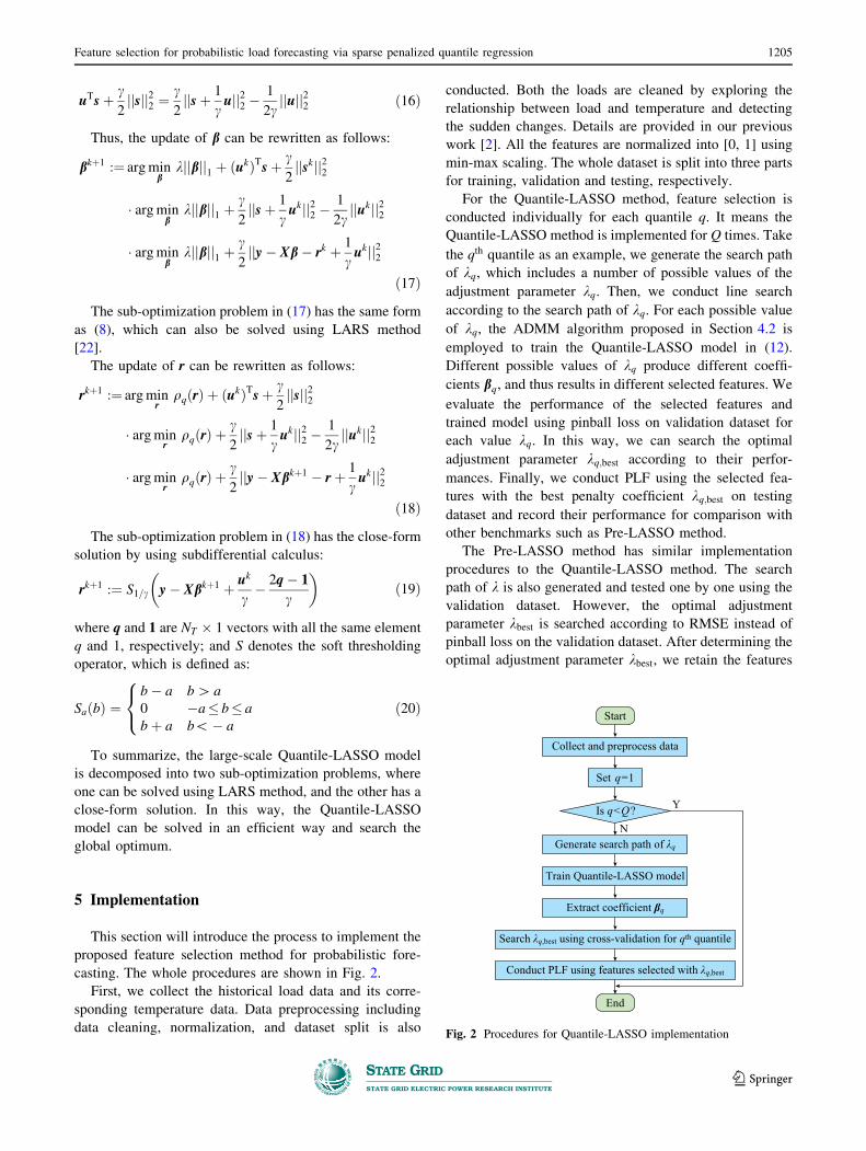
This section will introduce the process to implement the
proposed feature selection method for probabilistic fore-
casting. The whole procedures are shown in Fig. 2.
First, we collect the historical load data and its corre-
sponding temperature data. Data preprocessing including
data cleaning, normalization, and dataset split is also
conducted. Both the loads are cleaned by exploring the
relationship between load and temperature and detecting
the sudden changes. Details are provided in our previous
work [2]. All the features are normalized into [0, 1] using
min-max scaling. The whole dataset is split into three parts
for training, validation and testing, respectively.
For the Quantile-LASSO method, feature selection is
conducted individually for each quantile q. It means the
Quantile-LASSO method is implemented for Q times. Take
the qth quantile as an example, we generate the search path
of kq, which includes a number of possible values of the
adjustment parameter kq. Then, we conduct line search
according to the search path of kq. For each possible value
of kq, the ADMM algorithm proposed in Section 4.2 is
employed to train the Quantile-LASSO model in (12).
Different possible values of kq produce different coeffi-
cients bq, and thus results in different selected features. We
evaluate the performance of the selected features and
trained model using pinball loss on validation dataset for
each value kq. In this way, we can search the optimal
adjustment parameter kq;best according to their perfor-
mances. Finally, we conduct PLF using the selected fea-
tures with the best penalty coefficient kq;best on testing
dataset and record their performance for comparison with
other benchmarks such as Pre-LASSO method.
The Pre-LASSO method has similar implementation
procedures to the Quantile-LASSO method. The search
path of k is also generated and tested one by one using the
validation dataset. However, the optimal adjustment
parameter kbest is searched according to RMSE instead of
pinball loss on the validation dataset. After determining the
optimal adjustment parameter kbest, we retain the features
Collect and preprocess data
Set q=1
q<sI ?Q
Generate search path of λq
End
Start
N
Train Quantile-LASSO model
Extract coefficient βq
Search λq,best using cross-validation for qth quantile
Conduct PLF using features selected with λq,best
Y
Fig. 2 Procedures for Quantile-LASSO implementation
Feature selection for probabilistic load forecasting via sparse penalized quantile regression 1205
123
with non-zero coefficients to train the quantile regression
model on validation dataset and test the performance on the
testing dataset. For the Pre-LASSO method, the quantile
regression model for different quantiles uses the same
selected features.
After the two methods have been trained and validated,
we compare the performances of the two methods on the
same testing dataset in terms of pinball loss.
6 Case studies
6.1 Experiment setups
The load and temperature data used in the case studies
are from GEFCom 2012, of which the basic information is
introduced in Section 2. We choose three-year load and
temperature data from 2005 to 2007 as the training dataset,
first half-year data of 2008 as the validation dataset, and the
second half-year data of 2008 as the test dataset, which
means the final performance of the load forecasting is
evaluated on the second half-year data of 2008.
We use average quantile score (AQS) to evaluate the
performance of the proposed and competing methods. AQS
is defined as the average of the pinball loss of all the
quantiles:
SAQS ¼1
QNT
XQ
q¼1
XNT
t¼1
qqðyq;t � ytÞ ð21Þ
where yq;t denotes the forecasted qth quantile of the load. A
total of 9 quantiles 0:1; 0:2; . . .; 0:9, which are denoted as
q1; q2; . . .; q9, are used to form the probabilistic forecasts in
this paper. Since the proposed feature selection is designed
for linear regression model, two base competing methods
are the original linear quantile regression and the linear
quantile regression based on Pre-LASSO. The base fore-
casting model is illustrated in Section 2 to consider the
recency effects of temperature on loads. There are two
variables to be determined: the number of lagged days ND
and the number of lagged hours NH . We choose two
variable pair ðND;NHÞ as (3, 4) and (7, 12) , respectively,
in our case studies, which are denoted as D3-H4 model and
D7-H12 model. The search path of kq in Quantile-LASSO
model and k in Pre-LASSO model for the L1-norm penalty
is the same for both D3-H4 model and D7-H12 model. If
the recency-effect model is D3-H4 model or D7-H12
model, we have 1019 or 2279 features to be selected,
respectively, without consideration of intercept according
to (5). Neural network and gradient boosting regression
tree are commonly used in powerful regression models for
load forecasting. They have been widely used in GEFCom
2012 and 2014 [18, 23]. To show the superiority of the
MLR model for load forecasting, these two nonlinear
quantile regression models, QRNN [24] and QGBRT [25]
with default parameters are also tested for comparison.
6.2 Results
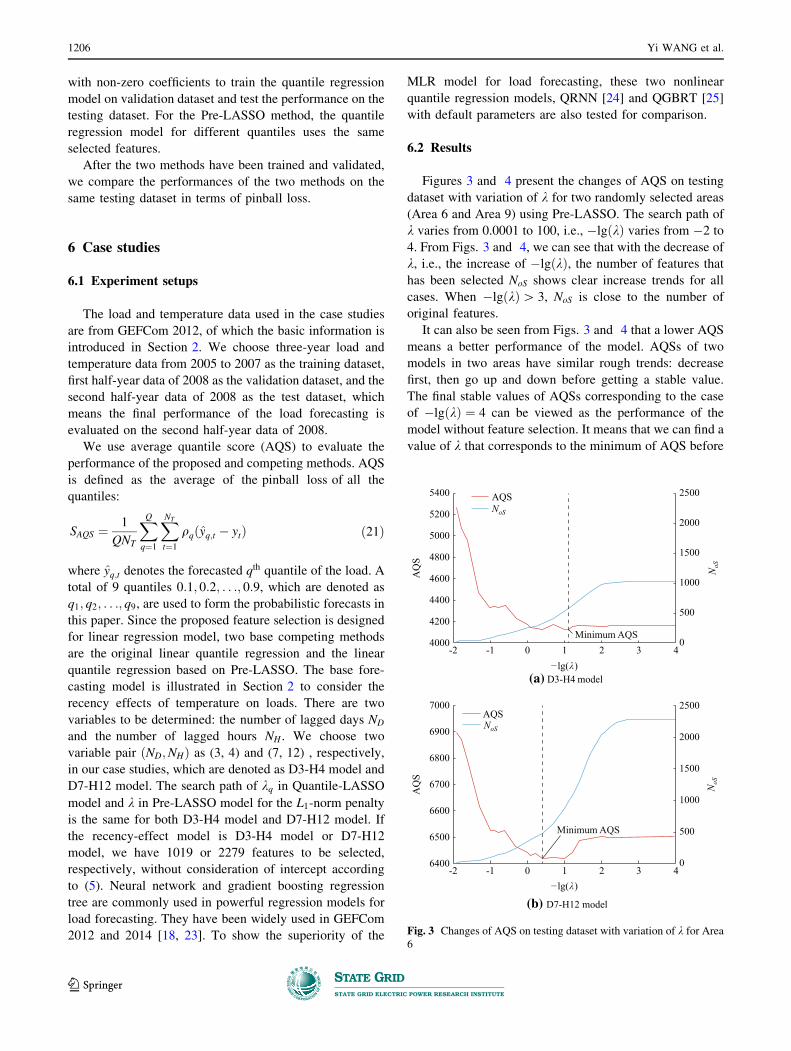
Figures 3 and 4 present the changes of AQS on testing
dataset with variation of k for two randomly selected areas
(Area 6 and Area 9) using Pre-LASSO. The search path of
k varies from 0.0001 to 100, i.e., �lgðkÞ varies from �2 to
4. From Figs. 3 and 4, we can see that with the decrease of
k, i.e., the increase of �lgðkÞ, the number of features that
has been selected NoS shows clear increase trends for all
cases. When �lgðkÞ[ 3, NoS is close to the number of
original features.
It can also be seen from Figs. 3 and 4 that a lower AQS
means a better performance of the model. AQSs of two
models in two areas have similar rough trends: decrease
first, then go up and down before getting a stable value.
The final stable values of AQSs corresponding to the case
of �lgðkÞ ¼ 4 can be viewed as the performance of the
model without feature selection. It means that we can find a
value of k that corresponds to the minimum of AQS before
AQ
S
−lg(λ)(a) D3-H4 model
(b) D7-H12 model
2500
2000
1500
1000
500
0
5400
5200
5000
4800
4600
4400
4200
4000-2 -1 0 1 2 3 4
AQS
Minimum AQS
AQ
S
−lg(λ)
NoS
NoS
NoS
NoS
2500
2000
1500
1000
500
0
7000
6900
6800
6700
6600
6500
6400-2 -1 0 1 2 3 4
AQS
Minimum AQS
Fig. 3 Changes of AQS on testing dataset with variation of k for Area6
1206 Yi WANG et al.
123
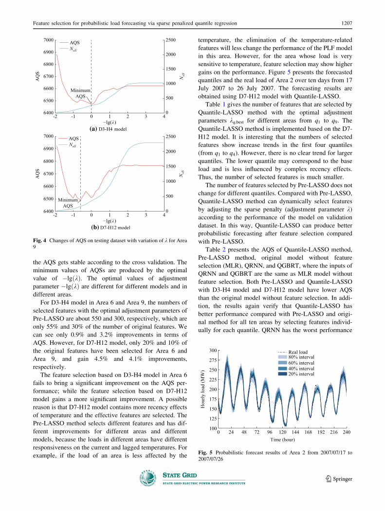
the AQS gets stable according to the cross validation. The
minimum values of AQSs are produced by the optimal
value of �lgðkÞ. The optimal values of adjustment
parameter �lgðkÞ are different for different models and in
different areas.
For D3-H4 model in Area 6 and Area 9, the numbers of
selected features with the optimal adjustment parameters of
Pre-LASSO are about 550 and 300, respectively, which are
only 55% and 30% of the number of original features. We
can see only 0.9% and 3.2% improvements in terms of
AQS. However, for D7-H12 model, only 20% and 10% of
the original features have been selected for Area 6 and
Area 9, and gain 4.5% and 4.1% improvements,
respectively.
The feature selection based on D3-H4 model in Area 6
fails to bring a significant improvement on the AQS per-
formance; while the feature selection based on D7-H12
model gains a more significant improvement. A possible
reason is that D7-H12 model contains more recency effects
of temperature and the effective features are selected. The
Pre-LASSO method selects different features and has dif-
ferent improvements for different areas and different
models, because the loads in different areas have different
responsiveness on the current and lagged temperatures. For
example, if the load of an area is less affected by the
temperature, the elimination of the temperature-related
features will less change the performance of the PLF model
in this area. However, for the area whose load is very
sensitive to temperature, feature selection may show higher
gains on the performance. Figure 5 presents the forecasted
quantiles and the real load of Area 2 over ten days from 17
July 2007 to 26 July 2007. The forecasting results are
obtained using D7-H12 model with Quantile-LASSO.
Table 1 gives the number of features that are selected by
Quantile-LASSO method with the optimal adjustment
parameters kq;best for different areas from q1 to q9. The
Quantile-LASSO method is implemented based on the D7-
H12 model. It is interesting that the numbers of selected
features show increase trends in the first four quantiles
(from q1 to q4). However, there is no clear trend for larger
quantiles. The lower quantile may correspond to the base
load and is less influenced by complex recency effects.
Thus, the number of selected features is much smaller.
The number of features selected by Pre-LASSO does not
change for different quantiles. Compared with Pre-LASSO,
Quantile-LASSO method can dynamically select features
by adjusting the sparse penalty (adjustment parameter k)according to the performance of the model on validation
dataset. In this way, Quantile-LASSO can produce better
probabilistic forecasting after feature selection compared
with Pre-LASSO.
Table 2 presents the AQS of Quantile-LASSO method,
Pre-LASSO method, original model without feature
selection (MLR), QRNN, and QGBRT, where the inputs of
QRNN and QGBRT are the same as MLR model without
feature selection. Both Pre-LASSO and Quantile-LASSO
with D3-H4 model and D7-H12 model have lower AQS
than the original model without feature selection. In addi-
tion, the results again verify that Quantile-LASSO has
better performance compared with Pre-LASSO and origi-
nal method for all ten areas by selecting features individ-
ually for each quantile. QRNN has the worst performance
AQ
S
−lg(λ)(a) D3-H4 model
(b) D7-H12 model
2500
2000
1500
1000
500
0
7000
6900
6800
6700
6600
6500
6400-2 -1 0 1 2 3 4
AQS
MinimumAQS
AQ
S
−lg(λ)
NoS
NoS
NoS
NoS
2500
2000
1500
1000
500
0
7000
6900
6800
6700
6600
6500
6400-2 -1 0 1 2 3 4
AQS
MinimumAQS
Fig. 4 Changes of AQS on testing dataset with variation of k for Area9
275
250
225
175
150
125
200
1000 24 48 72 96 120
Time (hour)
Hou
rly lo
ad (M
W)
144 168 192 216 240
300 Real load80% interval60% interval40% interval20% interval
Fig. 5 Probabilistic forecast results of Area 2 from 2007/07/17 to
2007/07/26
Feature selection for probabilistic load forecasting via sparse penalized quantile regression 1207
123
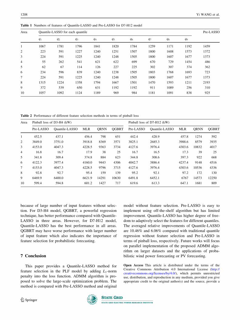
because of large number of input features without selec-
tion. For D3-H4 model, QGBRT, a powerful regression
technique, has better performance compared with Quantile-
LASSO in three areas. However, for D7-H12 model,
Quantile-LASSO has the best performance in all areas.
QGBRT may have worse performance with larger number
of input feature which also indicates the importance of
feature selection for probabilistic forecasting.
7 Conclusion
This paper provides a Quantile-LASSO method for
feature selection in the PLF model by adding L1-norm
penalty into the loss function. ADMM algorithm is pro-
posed to solve the large-scale optimization problem. The
method is compared with Pre-LASSO method and original
model without feature selection. Pre-LASSO is easy to
implement using off-the-shelf algorithm but has limited
improvement. Quantile-LASSO has higher degree of free-
dom to adaptively select the features for different quantiles.
The averaged relative improvements of Quantile-LASSO
are 10.46% and 6.06% compared with traditional quantile
regression without feature selection and Pre-LASSO in
terms of pinball loss, respectively. Future works will focus
on parallel implementation of the proposed ADMM algo-
rithm on larger datasets and the applications of proba-
bilistic wind power forecasting or PV forecasting.
Open Access This article is distributed under the terms of the
Creative Commons Attribution 4.0 International License (http://
creativecommons.org/licenses/by/4.0/), which permits unrestricted
use, distribution, and reproduction in any medium, provided you give
appropriate credit to the original author(s) and the source, provide a
Table 2 Performance of different feature selection methods in terms of pinball loss
Area Pinball loss of D3-H4 (kW) Pinball loss of D7-H12 (kW)
Pre-LASSO Quantile-LASSO MLR QRNN QGBRT Pre-LASSO Quantile-LASSO MLR QRNN QGBRT
1 452.5 437.1 456.4 798 651 442.4 428.9 457.8 1274 592
2 3849.0 3751.0 3918.8 8369 3571 3825.1 2685.3 3988.6 8579 3935
3 4153.0 4047.3 4228.5 9363 3734 4127.6 3976.4 4303.6 10832 4017
4 16.8 16.7 17.9 38 25 16.7 16.5 17.3 39 25
5 341.8 309.4 374.8 884 623 344.8 308.6 397.3 922 668
6 4122.3 3977.4 4160.0 9443 4306 4042.7 3886.4 4237.4 9148 4516
7 4153.0 4047.3 4228.5 9796 3715 4127.6 3976.4 4303.6 10536 4336
8 92.8 92.7 95.4 159 139 95.2 92.1 97.2 172 130
9 6469.9 6400.0 6621.9 14291 10630 6491.8 6452.1 6767 14573 12250
10 599.4 594.8 601.2 1427 717 619.6 613.3 647.1 1681 809
Table 1 Numbers of features of Quantile-LASSO and Pre-LASSO for D7-H12 model
Area Quantile-LASSO for each quantile Pre-LASSO
q1 q2 q3 q4 q5 q6 q7 q8 q9
1 1067 1781 1796 1841 1820 1784 1259 1171 1192 1459
2 223 591 1227 1240 1251 1507 1800 1608 1573 1372
3 224 591 1225 1240 1248 1505 1800 1607 1677 1373
4 55 262 541 621 622 699 670 729 1454 486
5 62 67 114 126 227 225 302 307 374 362
6 234 596 839 1240 1238 1505 1803 1768 1693 723
7 224 591 1225 1240 1248 1505 1800 1607 1677 1373
8 1315 1224 1358 1794 1667 1501 1470 1593 1211 2193
9 372 539 650 631 1192 1192 911 1089 256 310
10 1057 1092 1124 1189 969 984 1181 1091 838 925
1208 Yi WANG et al.
123
link to the Creative Commons license, and indicate if changes were
made.
Acknowledgement This work was supported by National Key R&D
Program of China (No. 2016YFB0900100).
References
[1] Hong T, Fan S (2016) Probabilistic electric load forecasting: a
tutorial review. Int J Forecast 32(3):914–938
[2] Gan D, Wang Y, Yang S et al (2018) Embedding based quantile
regression neural network for probabilistic load forecasting.
J Mod Power Syst Clean Energy 6(2):244–254
[3] Zhang W, Quan H, Srinivasan D (2018) An improved quantile
regression neural network for probabilistic load forecasting.
IEEE Trans Smart Grid. https://doi.org/10.1109/TSG.2018.
2859749
[4] Wang Y, Zhang N, Chen Q et al (2018) Data-driven proba-
bilistic net load forecasting with high penetration of behind-the-
meter PV. IEEE Trans Power Syst 33(3):3255–3264
[5] Wang Y, Zhang N, Kang C et al (2018) An efficient approach to
power system uncertainty analysis with high-dimensional
dependencies. IEEE Trans Power Syst 33(3):2984–2994
[6] He Y, Xu Q, Wan J et al (2016) Short-term power load prob-
ability density forecasting based on quantile regression neural
network and triangle kernel function. Energy 114:498–512
[7] Xie J, Hong T (2018) Temperature scenario generation for
probabilistic load forecasting. IEEE Trans Smart Grid
9(3):1680–1687
[8] Liu B, Nowotarski J, Hong T et al (2017) Probabilistic load
forecasting via quantile regression averaging on sister forecasts.
IEEE Trans Smart Grid 8(2):730–737
[9] Xie J, Hong T, Laing T et al (2017) On normality assumption in
residual simulation for probabilistic load forecasting. IEEE
Trans Smart Grid 8(3):1046–1053
[10] Wang Y, Zhang N, Tan Y et al (2018) Combining probabilistic
load forecasts. IEEE Trans Smart Grid. https://doi.org/10.1109/
TSG.2018.2833869
[11] Wang Y, Chen Q, Hong T et al (2019) Review of smart meter
data analytics: applications, methodologies, and challenges.
IEEE Trans Smart Grid 10(3):3125–3148
[12] Arora S, Taylor JW (2016) Forecasting electricity smart meter
data using conditional kernel density estimation. Omega
59:47–59
[13] Taieb SB, Huser R, Hyndman RJ et al (2016) Forecasting
uncertainty in electricity smart meter data by boosting additive
quantile regression. IEEE Trans Smart Grid 7(5):2448–2455
[14] Shepero M, Meer DVD, Munkhammar J et al (2018) Residential
probabilistic load forecasting: a method using gaussian process
designed for electric load data. Appl Energy 218:159–172
[15] Tibshirani R (2011) Regression shrinkage and selection via the
lasso. J R Stat Soc 73(3):267–288
[16] Xie J, Hong T (2018) Variable selection methods for proba-
bilistic load forecasting: empirical evidence from seven states of
the united states. IEEE Trans Smart Grid 9(6):6039–6046
[17] Boyd S, Parikh N, Chu E et al (2010) Distributed optimization
and statistical learning via the alternating direction method of
multipliers. Found Trends Mach Learn 3(1):1–122
[18] Hong T, Pinson P, Fan S (2014) Global energy forecasting
competition 2012. Int J Forecast 30(2):357–363
[19] Hong T (2010) Short term electric load forecasting. Disserta-
tion, North Carolina State University
[20] Wang P, Liu B, Hong T (2016) Electric load forecasting with
recency effect: a big data approach. Int J Forecast
32(3):585–597
[21] Tibshirani R (1996) Regression shrinkage and selection via the
LASSO. J R Stat Soc Ser B (Methodol) 58(1):267–288
[22] Efron B, Hastie T, Johnstone I et al (2004) Least angle
regression. Ann Stat 32(2):407–451
[23] Hong T, Pinson P, Fan S et al (2016) Probabilistic energy
forecasting: global energy forecasting competition 2014 and
beyond. Int J Forecast 32(3):896–913
[24] Cannon AJ (2011) Quantile regression neural networks:
implementation in r and application to precipitation downscal-
ing. Comput Geosci 37(9):1277–1284
[25] Ridgeway G (2007) Generalized boosted models: a guide to the
gbm package. https://www.docin.com/p-1477403664.html..
Accessed 3 Aug 2007
Yi WANG received the B.S. degree from the Department of
Electrical Engineering in Huazhong University of Science and
Technology (HUST), Wuhan, China, in 2014, and the Ph.D. degree
in Tsinghua University, Beijing, China, in 2019. He was also a
visiting student researcher at the University of Washington, Seattle,
USA. He is currently a postdoctoral researcher in ETH Zurich,
Switzerland. His research interests include data analytics in smart grid
and multiple energy systems.
Dahua GAN received the B.S. degree from the Electrical Engineer-
ing Department of Tsinghua University, Beijing, China, in 2017. His
research interests include load forecasting and power markets.
Ning ZHANG received the B.S. and Ph.D. degrees from the
Electrical Engineering Department of Tsinghua University, Beijing,
China, in 2007 and 2012, respectively. He is currently an associate
professor at the Tsinghua University. His research interests include
multiple energy systems integration, renewable energy, and power
system planning and operation.
Le XIE received the B.E. degree in electrical engineering from
Tsinghua University, Beijing, China, in 2004, the M.S. degree in
engineering science from Harvard University, Cambridge, USA, in
2005, and the Ph.D. degree from the Department of Electrical and
Computer Engineering, Carnegie Mellon University, Pittsburgh,
USA, in 2009. He is currently a professor with the Department of
Electrical and Computer Engineering, Texas A&M University,
College Station, USA. His research interests include modeling and
control of large-scale complex systems, smart grid application with
renewable energy resources, and electricity markets.
Chongqing KANG received the Ph.D. degree from the Department
of Electrical Engineering in Tsinghua University, Beijing, China, in
1997. He is currently a professor in Tsinghua University. His research
interests include power system planning, power system operation,
renewable energy, low carbon electricity technology and load
forecasting.
Feature selection for probabilistic load forecasting via sparse penalized quantile regression 1209
123