FEBio Workshop #2Multiphasic Materials

Gerard Ateshian

Steve Maas

Jeff Weiss

Biphasic Materials

• Mixture

– Porous deformable solid

– Interstitial fluid

• Assumptions

– Quasi-static analyses

– Incompressible solid matrix skeleton

– Incompressible interstitial fluid

– Solid matrix pores can lose or gain fluid volume

Biphasic Equations• Mixture stress

– fluid pressure

– effective stress

– momentum balance

• Mixture velocity

– solid velocity

– fluid flux relative to solid

– mass balance

• Fluid momentum

– hydraulic permeability

p

vs + w

vs

w

q = w×da div vs + w( ) = 0 da

n

w

w = -k ×grad p

k

Constitutive Relations

• Effective stress

– Compressible solid

– Strain energy density

– Deformation gradient

• Hydraulic permeability

– Constant or strain-dependent

– Invariant isotropic, referentially isotropic, referentially transversely isotropic, referentially orthotropic

Y = Y C( ) F, J = detF, C = F

T ×F

k

Biphasic FEA

• Virtual work integral

– virtual solid velocity

– virtual fluid pressure

• Internal and external work

• Natural BCs

dW = dWext -dWint

d v

d p

dWext = d v×t da

¶vò + d p wnda

¶vò

wn= w×n

Biphasic Boundary Conditions

• Natural BCs

– mixture traction

– normal fluid flux

• Essential BCs

– solid displacement

– fluid pressure

• Example

– Indentation

wn= w×n

u

p

u = 0 wn= 0

p = 0 t = 0

u

n= u

at( )

wn= 0

Biphasic Indentation

• Indenter– Flat-ended

– Rigid

– Impermeable

– Frictionless

– Implicit

• Biphasic Layer– Rigid substrate

– Impermeable substrate

– Biased mesh

Biphasic Indentation

• Boundary Conditions

– Bottom

– Side

– Top (outer)

– Top (inner)

• Must Points

• Full-Newton iterations

• Non-symmetric matrix

Biphasic Indentation

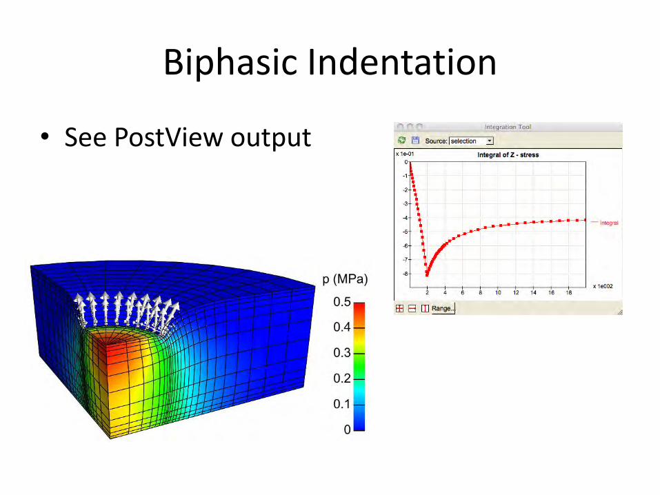
• See PostView output

Axisymmetric Problems

• Use wedge geometry

• Add rigid symmetry plane

• Use “Tension-compression contact”

– symmetry plane = master

– biphasic surface = slave

– auto-penalty on

– penalty = 104

Fluid Pressure on Free Surface

• Mixed BCs

– pressure:

– mixture traction:

– normal mixture traction:

– or normal effective traction

p = p

at( )

t

n= t×n = - p

at( )

p = p

at( )

tn

e = te ×n = 0

tn= - p

at( ) or t

e

n = 0

Example:Pressure-driven

permeation

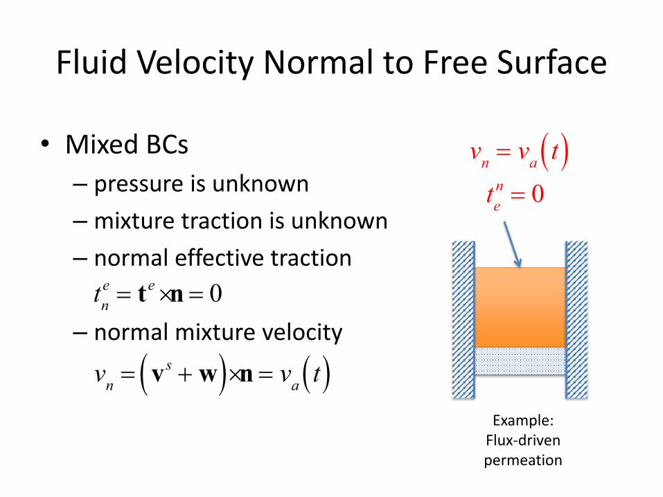
Fluid Velocity Normal to Free Surface

• Mixed BCs

– pressure is unknown

– mixture traction is unknown

– normal effective traction

– normal mixture velocity

v

n= v

at( )

tn

e = te ×n = 0

te

n = 0

v

n= v

s + w( )×n = va

t( )Example:

Flux-drivenpermeation

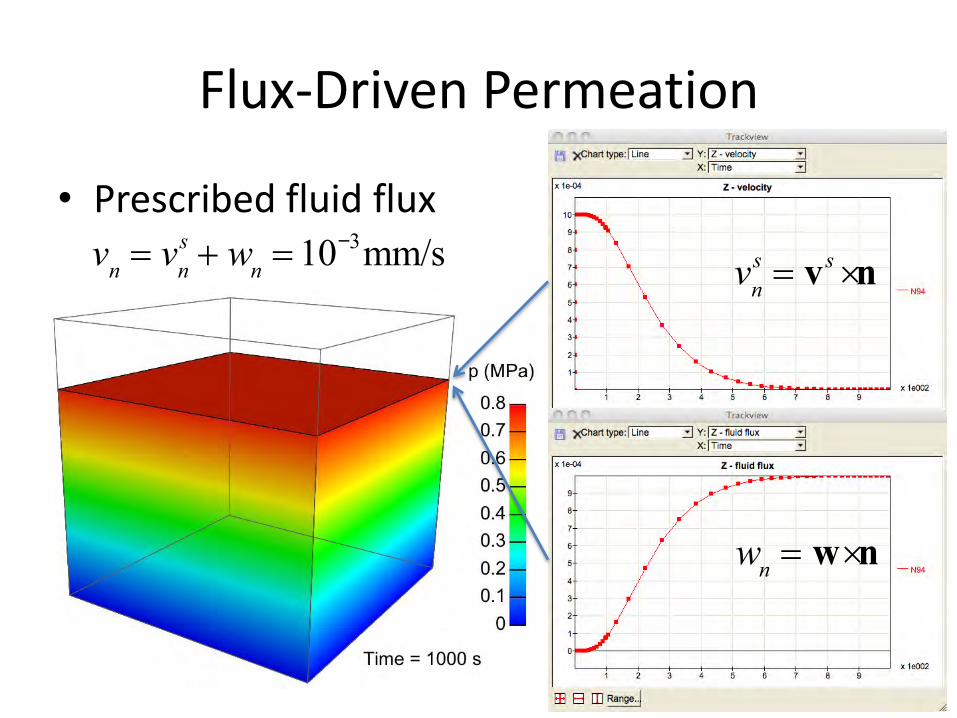
Flux-Driven Permeation

• Prescribed fluid flux

vn= v

n

s + wn=10-3mm/s

vn

s = vs ×n

wn= w×n

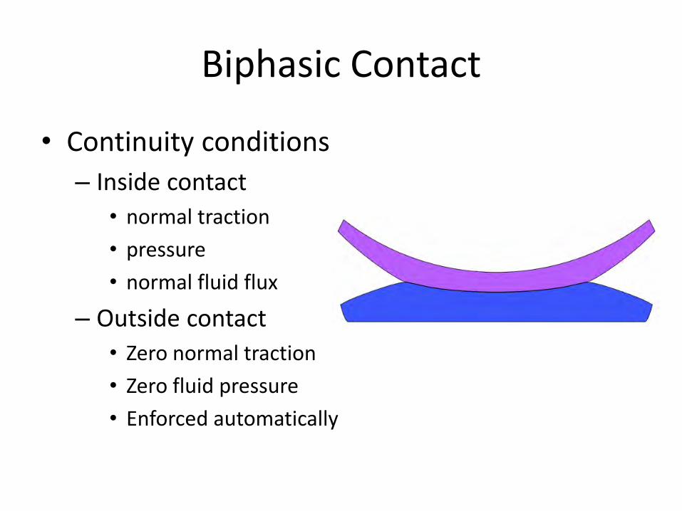
Biphasic Contact

• Continuity conditions

– Inside contact

• normal traction

• pressure

• normal fluid flux

– Outside contact

• Zero normal traction

• Zero fluid pressure

• Enforced automatically

Biphasic Interface Settings

• Biphasic-on-biphasic

– auto-penalty on

– penalty factor 1≤pf≤10

– two-pass

– non-symmetric stiffness

– biased mesh

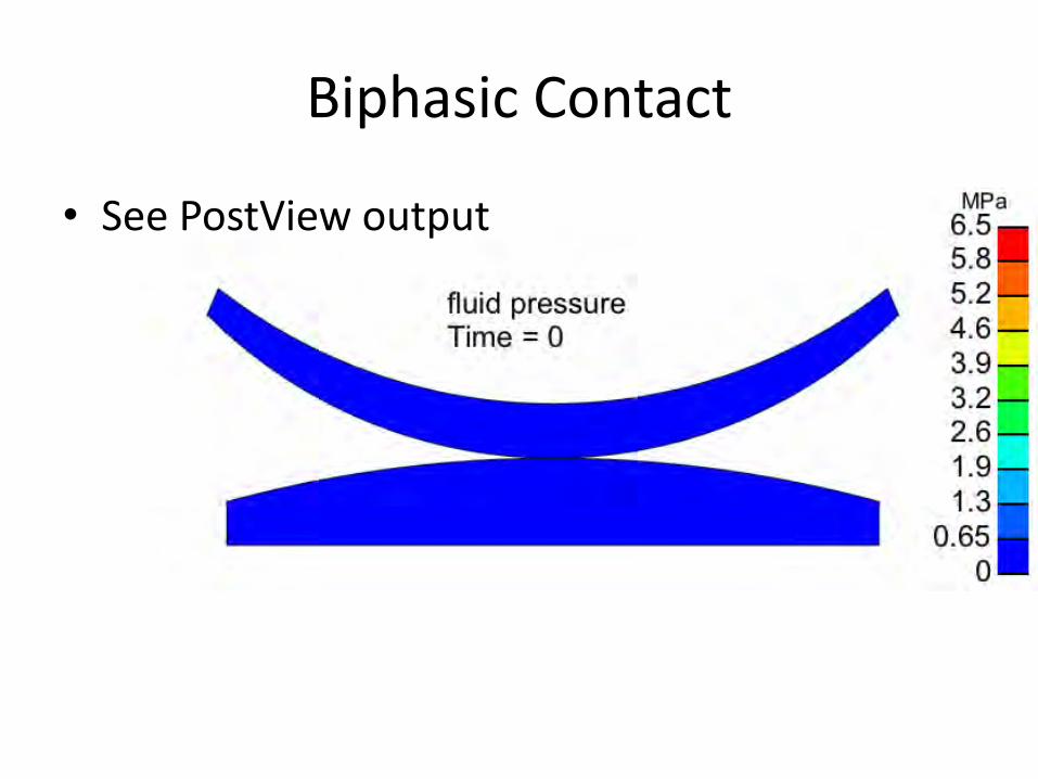
Biphasic Contact

• See PostView output

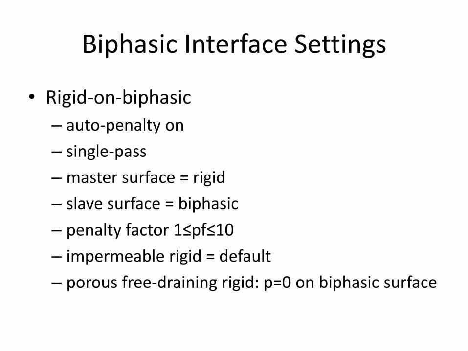
Biphasic Interface Settings

• Rigid-on-biphasic

– auto-penalty on

– single-pass

– master surface = rigid

– slave surface = biphasic

– penalty factor 1≤pf≤10

– impermeable rigid = default

– porous free-draining rigid: p=0 on biphasic surface

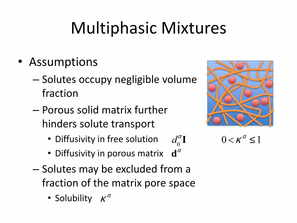
Multiphasic Mixtures

• Assumptions

– Solutes occupy negligible volume fraction

– Porous solid matrix further hinders solute transport

• Diffusivity in free solution

• Diffusivity in porous matrix

– Solutes may be excluded from a fraction of the matrix pore space

• Solubility

d0aI

da

0 <k a £1

k a

Multiphasic Equations

• Mixture momentum

• Mixture mass balance

– Solvent volume flux relative to solid

• Solute mass balance

– Porosity

– Solute concentration (solution basis)

– Solute molar flux relative to solid

• Electroneutrality

– Solid fixed charge density

– Solute charge number

div vs + w( ) = 0

w

¶ j wca( )¶t

+ div ja +j wca

vs( ) = 0

ca

jw

ja

cF + zaca

aå = 0

cF

za

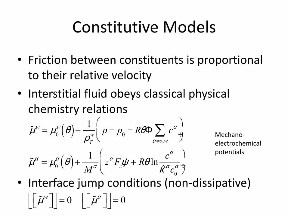
Constitutive Models

• Friction between constituents is proportional to their relative velocity

• Interstitial fluid obeys classical physical chemistry relations

• Interface jump conditions (non-dissipative)

mw = m0

w q( )+ 1r

T

wp - p0 - RqF ca

a¹s,wå

æ

èç

ö

ø÷

ma = m0

a q( )+ 1M a

za Fcy + Rq ln ca

k̂ ac0a

æ

èç

ö

ø÷

mwé

ëùû

éë

ùû= 0

maéë

ùû

éë

ùû= 0

Mechano-electrochemical potentials

Definitions

• Universal gas constant

• Faraday’s constant

• Absolute temperature

• Electric potential

• Solvent true density

• Osmotic coefficient

• Solute molar mass

• Solute activity coefficient

• Solute solubility

• Effective solubility

• Partition coefficient

rT

w

Ma

R

q

Fc

F

g a

k a

k̂a =k a g a

y

ka

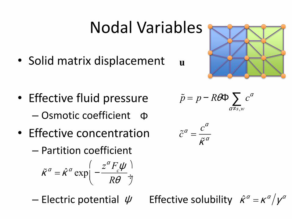
Nodal Variables

• Solid matrix displacement

• Effective fluid pressure

– Osmotic coefficient

• Effective concentration

– Partition coefficient

– Electric potential Effective solubility

u

p = p - RqF ca

a¹s,wå

ca =

ca

k a

k a = k̂ a exp -

za Fcy

Rq

æ

èç

ö

ø÷

F

y k̂a =k a g a

Solvent and Solute Fluxes

• Momentum balance for solvent & solutes

• Constitutive relations for and ma

w = -k × grad p + Rq

k a

d0a

da ×grad ca

a

åæ

èç

ö

ø÷

ja =k a

da × -j w grad ca +

ca

d0a

wæ

èç

ö

ø÷

k = k

-1 +Rq

j w

k aca

d0a

I -d

a

d0a

æ

èç

ö

ø÷

a

åé

ëêê

ù

ûúú

-1

mw

Fickian Diffusion

• Neutral solute

• Ideal solution

• Perfect solubility

• Effective concentration

• Boundary conditions

• Negligible osmotic pressure re solid elasticity

y = 0

F =1 ga =1

k a =1

ca = ca

caéë

ùû

éë

ùû= caé

ëùû

éë

ùû= 0

péë ùûé

ëùû = p - Rq ca

aåéë

ùû

éë

ùû= 0

2D Anisotropic FRAP• Fluorescence recover after photobleaching

• Anisotropic diffusivity

• Boundary & initial conditions

ux= 0

c = c*

uy= 0

c = c*

uz= 0

jn= 0

c t = 0( ) = c*

p t = 0( ) = p* - Rqc*

c t = 0( ) = 0

p t = 0( ) = p*

2D Anisotropic FRAP

Gel Osmotic Loading

• Osmotic pressure comparable to gel elasticity

• Imperfect solubility

• Alginate-like gel

• Dextran-like molecule

k a = 0.986

E ~ 6kPa

c* = 6mM Rqc* ~ 15kPa

c t = 0( ) = 0

p t = 0( ) = p*

c = c*

p = p* - Rqc*

tn= - p*

p* = 0Be smart!Initial conditions

Boundary conditions

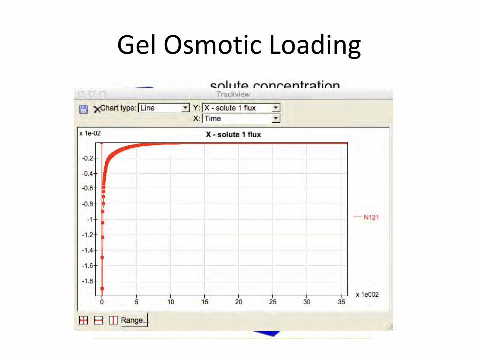
Gel Osmotic Loading

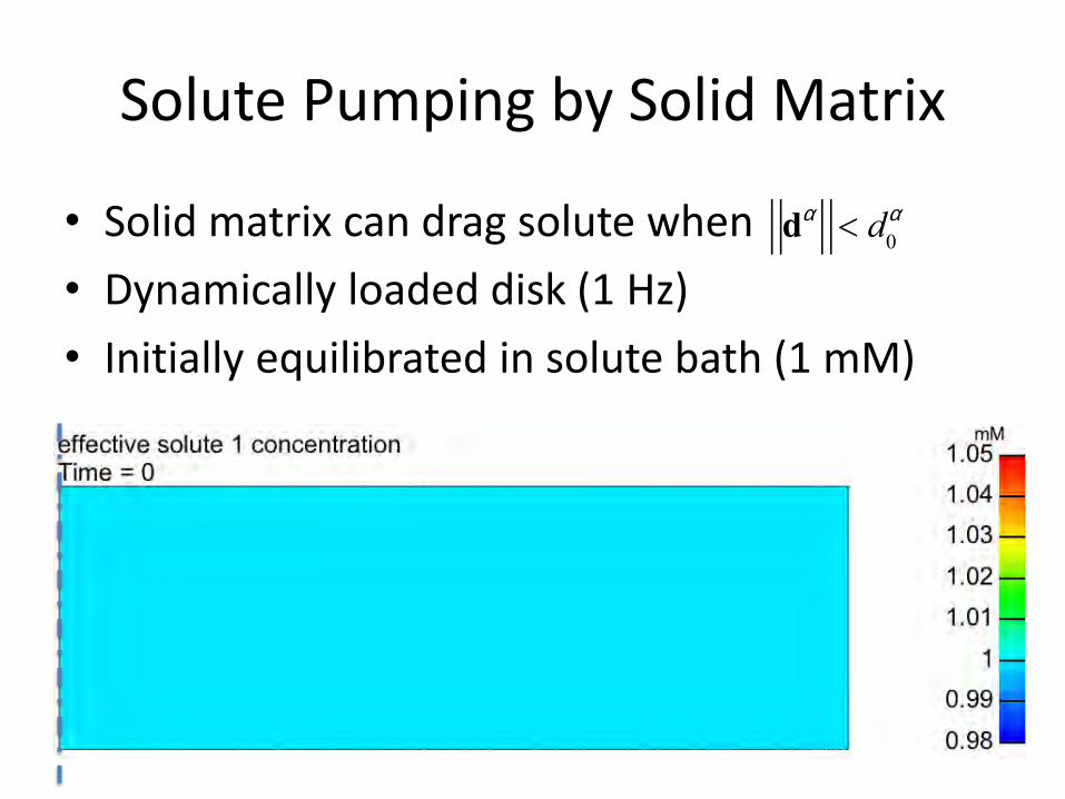
Solute Pumping by Solid Matrix

• Solid matrix can drag solute when

• Dynamically loaded disk (1 Hz)

• Initially equilibrated in solute bath (1 mM)

da < d0

a

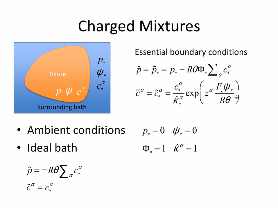
Charged Mixtures

• Ambient conditions

• Ideal bath

Tissue

Surrounding bath

y *

p*

c*a

p y ca

p = p* = p* - RqF* c*a

aå

ca = c*a =

c*a

k̂ *a

exp za Fcy *

Rq

æ

èçö

ø÷

p* = 0 y * = 0

F* =1 k̂ a =1

p = -Rq c*a

aåca = c*

a

Essential boundary conditions

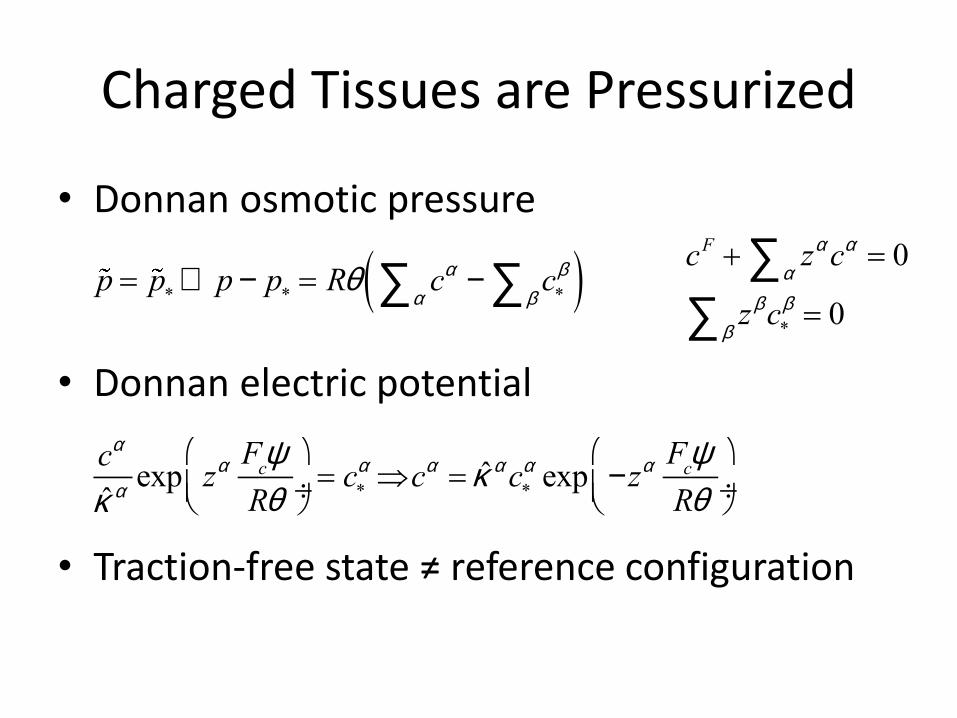
Charged Tissues are Pressurized

• Donnan osmotic pressure

• Donnan electric potential

• Traction-free state ≠ reference configuration

cF + za ca

aå = 0

zbc*b

bå = 0 p = p* Þ p - p* = Rq ca

aå - c*b

bå( )

ca

k̂ aexp za F

cy

Rq

æ

èçö

ø÷= c*

a Þca = k̂ ac*a exp -za F

cy

Rq

æ

èçö

ø÷

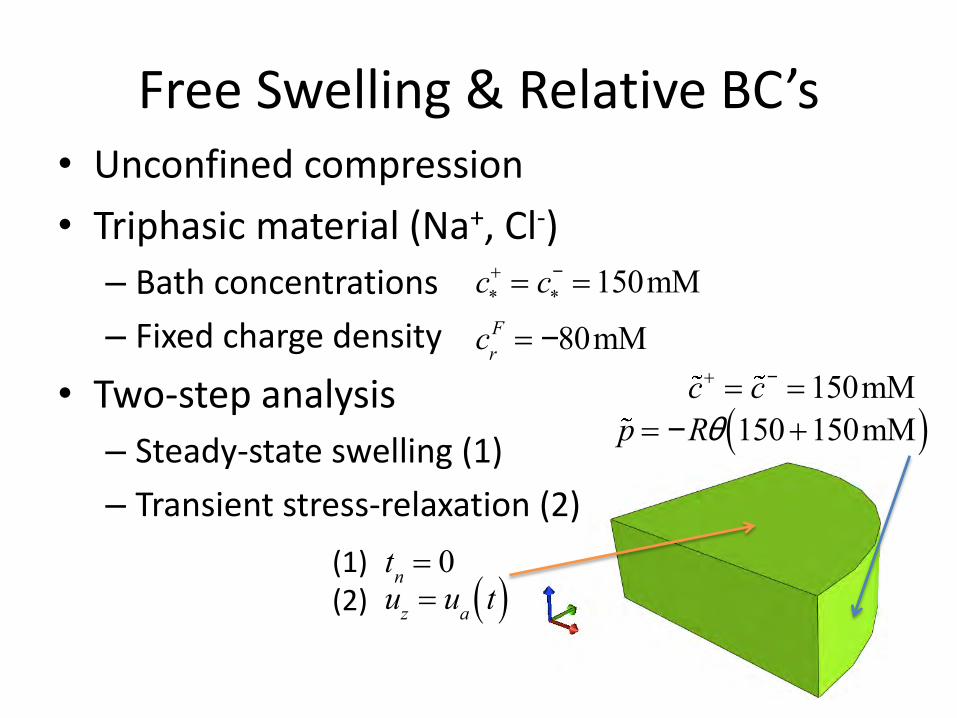
Free Swelling & Relative BC’s• Unconfined compression

• Triphasic material (Na+, Cl-)

– Bath concentrations

– Fixed charge density

• Two-step analysis

– Steady-state swelling (1)

– Transient stress-relaxation (2)

c*+ = c*

- =150mM

cr

F = -80mM

c+ = c- =150mM

p = -Rq 150+150mM( )

tn= 0

u

z= u

at( )

(1)(2)

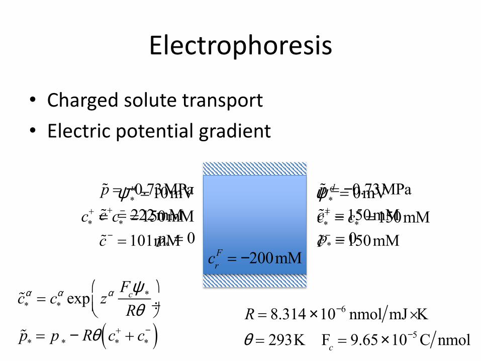
Electrophoresis

• Charged solute transport

• Electric potential gradient

y *d = 0mV y *

u =10mV

c*+ = c*

- =150mM

p* = 0 c*+ = c*

- =150mM

p* = 0

R = 8.314 ´10-6 nmol mJ×Kq = 293K F

c= 9.65´10-5 C nmol

c*

a = c*a exp za F

cy *

Rq

æ

èçö

ø÷

p* = p * - Rq c*+ + c*

-( )

cr

F = -200mM

p = -0.73MPac+ = 222mMc- = 101mM

p = -0.73MPac+ = 150mMc- = 150mM

Acknowledgments

• FEBio– www.febio.org

• National Institutes of Health– NIGMS GM083925– NIAMS AR060361– NIAMS AR043628

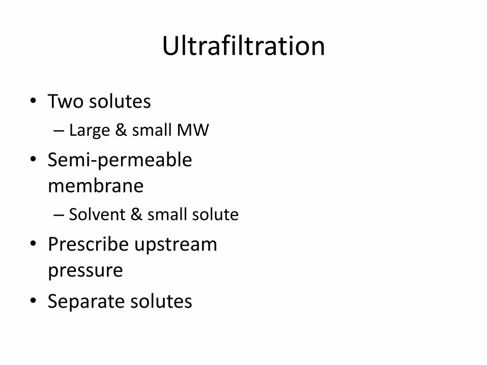
Ultrafiltration

• Two solutes

– Large & small MW

• Semi-permeable membrane

– Solvent & small solute

• Prescribe upstream pressure

• Separate solutes