Embed Size (px)
Citation preview
Federal Farm Subsidies
and
Agricultural Industrialization
Christopher Bartenstein
Thesis Advisor: John J Siegfried
Chris Bartenstein Economics Honors Thesis Spring, 2010
2
Contents
Abstract 1 Introduction to Industrial Agriculture and its Alternative
1.1 Measuring Agricultural Industrialization
2 Farm Subsidy Programs: a Threat to the Alternative Paradigm? 2.1 Modeling the Alternative Paradigm’s Perception of US Farm Subsidy Effects
3 Theory: Dissecting the Alternative-Paradigm Critique
3.1 The Subsidy Straitjacket 3.2 Risk, Industrial Farming, and Federal Subsidy Programs 3.3 Induced Innovation and Farming Habits 3.4 Modeling Theory 3.5 Aggregate Effects of Subsidy Programs vs. Farm Level Effects of Subsidy Programs
4 Empirical Analysis 4.1 Regression Models 4.2 Two Assumptions 4.3 Setting Appropriate Lags 4.4 Defining the Independent and Dependent Variables 4.5 Controls 5 Regressions (results) 5.1 Key 5.2 Regression #1 5.3 Regression #2 6 Analysis/Discussion 6.1 Discussion of Regression 1 6.2 Analysis of Regression 1 6.3 Discussion of Regression 2 6.4 Analysis of Regression 2 7 Conclusion
Appendices
Bibliography
Chris Bartenstein Economics Honors Thesis Spring, 2010
3
Abstract
My thesis explores the relationship between subsidy programs laid out in the 2002
farm bill and industrial farming practices. I hypothesize that farm policies have
encouraged high input, agro-chemical-dependent farming practices vis-à-vis more
sustainable farming practices. An empirical model based on agricultural census data
weakly supports this hypothesis and suggests the need for additional research into the
relationship between federal subsidy programs and agricultural industrialization.
1 Introduction to Industrial Agriculture and its Alternative
US agriculture underwent a series of major transformations over the course of the
20th century. Between 1932 and 2002, the percentage of the US population employed on
farms fell from 30% to 2%, signifying consolidation of farmland into larger operations
and substitution of capital and technology for labor. Meanwhile, productivity per unit of
land skyrocketed, food prices plummeted, and the US ran increasingly large food
surpluses. Throughout the century, farm operations also grew more specialized and
vertically integrated with downstream food processors and distributors.1 Agricultural
economists collectively refer to these developments as agricultural industrialization (AI).
1 “Vertical coordination (featuring integration of farm product marketing or input supply with production agriculture through integrated ownership, production contracts, or marketing contracts) now accounts for over 40% of farm output”
Luther Tweeten, Agrigultural Industrialization: For Better or Worst? (Anderson Chair Occasional Paper ESO #2404, Department of Agricultural, Environmental, and Development Economics, The Ohio State University, 1998), 2-3.
Chris Bartenstein Economics Honors Thesis Spring, 2010
4
Agricultural industrialization signifies the emergence of an agricultural system that
increasingly resembles modern non-food industries in the US. 2
Politicians and academics have often praised industrial agriculture (IA). Its
proponents point out that IA has provided cheap, abundant food and has freed up human
resources to fuel economic growth in the rest of the economy. However, in recent
decades IA has also become the subject of harsh criticism from environmentalists and a
growing subset of farmers and farm spectators. “Surface water pollution, groundwater
pollution, hypoxia zones, increased flooding, depletion of groundwater, air pollution,
excessive odors, climate change, loss of wildlife habitat, degradation of natural
ecosystems, loss of pollinators, loss of soil quality, and soil erosion” constitute a non-
comprehensive list of the environmental externalities attributed to IA by its detractors.3
Critics also charge IA with hastening the demise of family farms and vibrant rural
communities. Finally, many agro-ecologists doubt the long-term sustainability of
industrial agricultural production and raise long-term food security concerns. According
to one prominent agro-ecologist: 2 Agro-ecologist Stephen Gliessman notes the similarity between modern agriculture and industrial production in other industries, referring to industrial agriculture as “an industrial process in which plants assume the role of miniature factories: their output is maximized by supplying the appropriate inputs, their productive efficiency is increased by manipulation of their genes, and soil is simply the medium in which their roots are anchored…(two) interrelated goals (are espoused)…maximization of production and maximization of profit”
Stephen R. Gliessman, Agroecology: Ecological Processes in Sustainable Agriculture (CRC Press LLC, Boca Raton, Florida, 2000), 3.
Or, in the words of Luther Tweeten “larger operations can feature the scientific input, specialized resources, and low variable costs from production and marketing processes resembling those in nonfarm factories.”
Tweeten, Agricultural Industrialization: For Better or Worst?, 3.
3 Denns Keeney and Loni Kemp, A New Agricultural Policy for the United States (The Institute for Agriculture and Trade Policy and The Minnesota Project, July 2003; Produced for the North Atlantic Treaty Organization Advanced Research Workshop on Biodiversity Conservation and Rural Sustainability, Krakow, Poland, November 6, 2002), 11.
Chris Bartenstein Economics Honors Thesis Spring, 2010
5
“The techniques, innovations, practices, and policies that have allowed increases in productivity
have also undermined the basis for that productivity. They have overdrawn and degraded the
natural resources upon which agriculture depends—soil, water resources, and natural genetic
diversity. They have also created a dependence on nonrenewable fossil fuels and helped to forge a
system that increasingly takes the responsibility for growing food out of the hands of farmers and
farm workers, who are in the best position to be stewards of agricultural land. In short, modern
agriculture is unsustainable—it cannot continue to produce enough food for the global population
over the long term because it deteriorates the conditions that make agriculture possible.”4
According to Beus and Dunlap, an emergent paradigmatic rift polarizes the debate
over the future of agriculture in the United States. In their view, “the conventional
paradigm of large-scale, highly industrialized agriculture is being challenged by an
increasingly vocal alternative agriculture movement which advocates major shifts toward
a more ecologically sustainable agriculture.”5 Beus and Dunlap label these competing
perspectives the “conventional agriculture paradigm” and the “alternative agriculture
paradigm.” 6
To paint in large brushstrokes, the “alternative paradigm” promotes a system of
agriculture whereby many small farmers work in concert with the land by taking
advantage of synergies between diverse natural systems. A premium is placed on
sustaining/restoring environmental integrity and building/strengthening rural
4 Stephen R. Gliessman, Agroecology: The Ecology of Sustainable Food Systems, 2nd Edition (CPC Press, Boca Raton, Florida, 2007), 3.
5 Curtis Beus and Riley Dunlap, “Conventional versus Alternative Agriculture: The Paradigmatic Roots of the Debate,” Rural Sociology, 55, No 4, 1990, 590-616, 590.
6 Beus and Dunlap emphasize that the current alternative agriculture movement is not “just the latest manifestation of the ongoing struggle between agrarianism and industrial concentration…while some of the goals advocated by alternative agriculturalists are similar to those of past agrarian movements, it appears to be this core environmental grounding which has given alternative agriculture the momentum need to emerge as a legitimate movement”.
Ibid., 595.
Chris Bartenstein Economics Honors Thesis Spring, 2010
6
communities. Alternative farming methods require managerial experience and flexibility
in addition to a great deal of regular human labor and oversight. By contrast, the
“conventional (or industrial) paradigm” stresses the economic gains achieved through
economies of scale and predictability in terms of quantity and quality of output. The
premium placed on predictability and large-scale production entails routinized modes of
production, specialization, and relatively few farmers managing massive farm operations.
Because routinization and specialization run counter to the logic of the natural systems
harnessed by alternative farmers to restore soil fertility and protect crops, industrial
(conventional) farming relies heavily upon fertilizers and agrochemicals (e.g. pesticides,
herbicides, synthetic hormones, chemical growth agents etc.) for these purposes.
Although advocates of either paradigm view new technology as an effective means for
lowering both direct, economic costs of agricultural production and external,
social/environmental costs of agricultural production, conventional agriculturalists tend
to prioritize the former goal, whereas alternative agriculturalists tend to prioritize the
latter goal.7
1.1 Measuring Agricultural Industrialization
Although the conventional/alternative dichotomy neatly separates out the two
predominant, conceptually distinct frames of reference informing current beliefs and
preferences about US agriculture, actual agricultural practices in the United States are
much less easy to categorize. In his bestselling Omnivores Dilemma, Michael Pollan, a
staunch advocate of the alternative agricultural paradigm, identifies three of the most
7 See Appendix A: the table, taken from Beus and Dunlap, further contrasts these two competing paradigms.
Chris Bartenstein Economics Honors Thesis Spring, 2010
7
common patterns of food production in the United States: industrial agriculture, the big
organic operation, and the local self-sufficient farm.8 Mapping these three systems along
the conventional/alternative spectrum, industrial agriculture falls closely in line with the
conventional ideal; the local, self-sufficient farm closely resembles the alternative ideal;
the big organic operation resembles a rough compromise between the two ideals.
Although Pollan’s prototypes constitute three of the most popular and representative
models for farming in the United States, a wide variety of alternative farming
arrangements are conceivable and do exist. Less common arrangements fall at all points
along a continuum spanning between the conventional ideal (industrial agriculture) and
the alternative ideal (local, self-sufficient farms).
This is not, however, to suggest that the “industrial” (or “conventional”) and
“alternative” labels poorly characterize current agricultural conditions and divisions in
the US agricultural landscape. Although only a small portion of the farms in the United
States conform entirely to the industrial or to the alternative mold, theory suggests that
the suites of qualities attributed to each system are generally self-reinforcing and
therefore tend to be observed simultaneously. Empirical data supports this view. In a
1995 study investigating the contribution of agricultural industrialization to rural
stagnation, agricultural economist Dean MacCannell used the following measurements as
proxies for levels of agricultural industrialization:9
8 Michael Pollan, The Omnivore’s Dilemna (The Penguin Group, NY, NY, 2006).
9 Dean MacCannell, “Industrial Agriculture and Rural Community Degradation,” Agriculture and Community Change in the U.S. The Concgressional Research Reports (Underview Press, Boulder, CO, 1988), http://www.sarep.ucdavis.edu/newsltr/components/v2n3/sa-4.htm, 15-75 and 325-355.
Chris Bartenstein Economics Honors Thesis Spring, 2010
8
• the percent of farms in a county organized as corporations • farm size in acres in a county • the percent of farms in the county having more than $40,000 in sales • percent of farms with full-time hired labor • cost of hired labor per farm • cost of contract labor per farm • value of machinery per farm • cost of fertilizers per farm • costs of other chemicals per farm
Since IA shares an antonymous relationship with alternative agriculture, the same proxies
measure alternative agriculture. 10 Higher values for these proxies indicate IA, whereas a
lower value for each of these proxies indicates more alternative systems of agriculture.
In his study, MacCannell points out that “all of these variables show that, except
for size in acres, all measures of industrialization are strongly and positively correlated…
(suggesting) a single, system-wide pattern of alternative agriculture.”11 However,
MacCannell’s study is out of date. So, agricultural census data was manipulated to
generate more recent values for these proxies (and a few others). Data were collected for
eight proxies for industrialization and correlations between each pair were determined.12
The correlation coefficients are almost uniformly positive (very highly positive in some
cases), suggesting the collection of proxies does indeed identify a “single, system-wide
pattern of industrial agriculture.” Therefore, all correlated variables serve as legitimate
proxies for industrialization. Notably, “average operating fertilizer expense” has the
10 For purposes of simplicity, alternative agriculture is defined as the antithesis of industrial agriculture. In other words, alternative and industrial agriculture are considered in zero-sum terms. Increases in industrial agriculture are construed as decreases in alternative agriculture, and vice versa. The simplification makes sense because the two modes of agriculture have largely been defined by how they differ from one another.
11 Dean MacCannell, “Industrial Agriculture and Rural Community Degradation,” 37.
12 A correlation matrix for these proxies is found in Appendix C.
Chris Bartenstein Economics Honors Thesis Spring, 2010
9
highest mean correlation coefficient of the eight variables, suggesting it may be an
especially useful proxy if the other proxies are meaningful.
2.1 Farm Subsidy Programs: a Threat to the Alternative Paradigm?
Since the 1933 passage of the Agricultural Adjustment Act, a response to the
desperate situation of depression era farmers facing plummeting food prices, the United
States has maintained an aggressively interventionist farm subsidy program. Over the
decades, farm subsidies have served as a vehicle for launching a variety of political and
economic agendas. 13 The US government has not been unique in its support of domestic
agriculture. In the later half of the twentieth century, developed nations around the globe
spun out generous farm subsidy programs.
Conservationists have long criticized government intervention in agriculture.
Historically, they blamed government subsidies for promoting damaging levels of
intensification/overproduction and for encouraging unsustainable agricultural practices.
In the 1980’s and early 1990’s, agronomists produced a number of studies suggesting US
and EU subsidy programs of the period may have promoted structural shifts in the farm
sector toward more environmentally harmful, industrial modes of production. In support
of this case, observers of agricultural policy mobilize evidence of an apparent transition
toward more sustainable (and less industrial) farming practices in New Zealand
subsequent to its parliament’s decision to abolish all farm subsidies.
13 The declared objective of the Agricultural Adjustment Act was to restore farm income to pre-depression levels. Although sustaining “price parity” for an economically vulnerable farm population has been repeatedly cited since the 1930’s as grounds for payments, various other justifications for continued farm support have come in and out of vogue over the decades. Some of the most common justifications have included protecting the family farm, ensuring food security (by sustaining oversupply), and encouraging a favorable balance of trade.
Chris Bartenstein Economics Honors Thesis Spring, 2010
10
Since the early 1990’s, WTO pressures, changes in prevailing political currents,
and, notably, the arguments of environmentalists have led to major revisions in EU
Common Agricultural Policy and the three most recent iterations of the US Farm Bill.14
In light of these changes, much criticism originally brought to bear against farm subsidies
demands re-evaluation. However, advocates of the “alternative agriculture paradigm”
tend to overlook the tremendous variation in subsidy programs across space and time.15
They have appropriated conservationists’ historical disdain for subsidy programs,
rhetorically crucifying farm subsidies on the basis of outdated research and overly-
simplistic theories. The surging mainstream popularity of the alternative movement has
enabled questionable perceptions about subsidy programs to gain traction in the public
imagination. Op-ed’s abound in local and national periodicals accusing farm subsidies of
all order of evils. Said literature generally mobilizes little hard, coherent theory and less
empirical data in support of its claims. It is tempting to assume that the alternative
critique of farm subsidies amounts only to a vast collection of outdated, spurious memos
circulating within an echo chamber of ill-informed idealism. Appearances can be
deceptive. Concealed among the reams of junk theory are a few logically consistent,
though poorly studied theories predicting that modern subsidy programs will continue to 14 US Farm Bills are temporary, omnibus legislative acts which authorize the majority of federal farm subsidy programs. A new farm bill is passed approximately every five years.
15 Moreover, according to one agronomist, even “identical subsidy levels may have different impacts, e.g., on production and the environment, depending on the institutional framework and its particular implementation in a given country, but also related to the individual situation of a beneficiary e.g., characterized by production structure, natural disadvantages and environment. A complex relationship between such parameters often makes a simple analysis through the observation of environmental indicators a hopeless venture (i.e., time lags, unknown causal relationships, uncertainty).”
Markus F. Hofreither, Erwin Schmid, Franz Sinabell, “Phasing Out of Environmentally Harmful Subsidies: Consequences of the 2003 CAP Reform,” Prepared for presentation at the American Agricultural Economics Association Annual Meeting, Denver, CO, July 1-4, 2004. ageconsearch.umn.edu/bitstream/20169/1/sp04ho04.pdf, 6.
Chris Bartenstein Economics Honors Thesis Spring, 2010
11
encourage AI. This thesis aims to investigate the validity of the alternative-paradigm
critique of government subsidies.
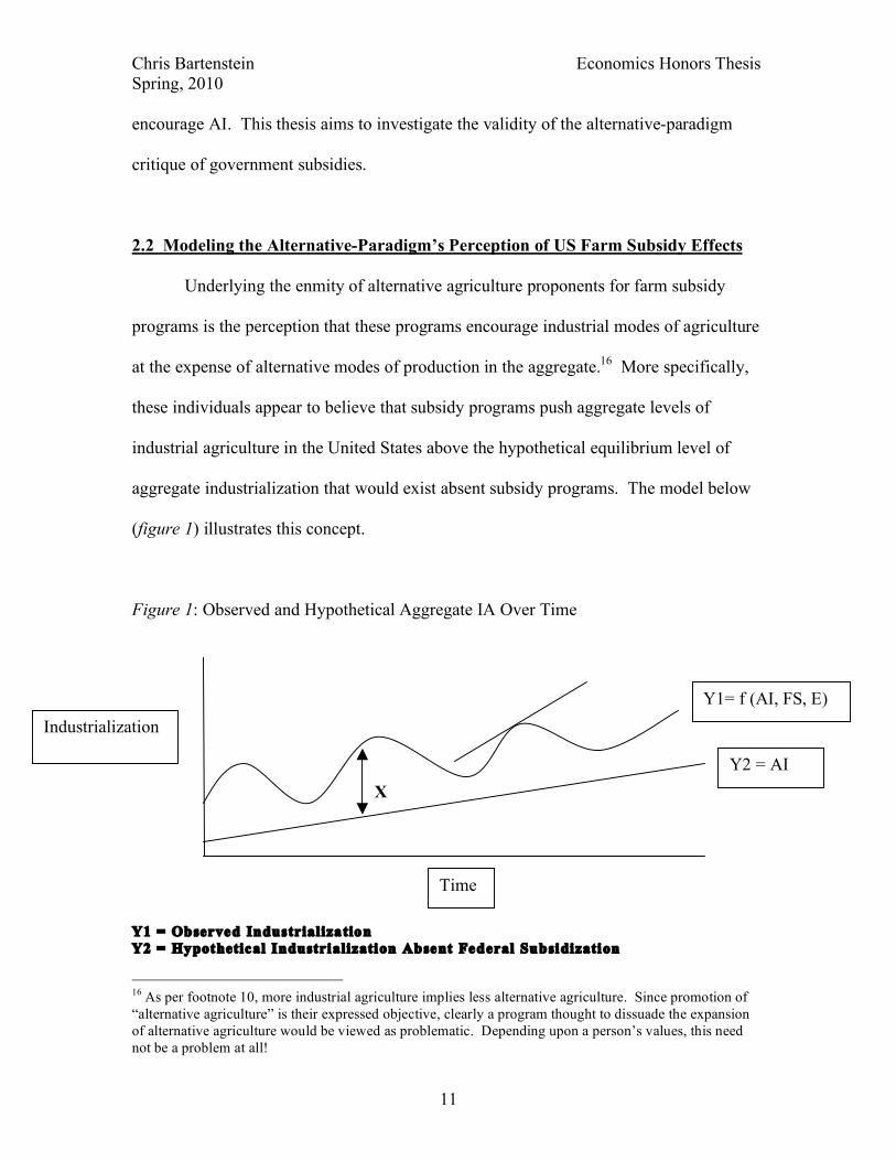
2.2 Modeling the Alternative-Paradigm’s Perception of US Farm Subsidy Effects
Underlying the enmity of alternative agriculture proponents for farm subsidy
programs is the perception that these programs encourage industrial modes of agriculture
at the expense of alternative modes of production in the aggregate.16 More specifically,
these individuals appear to believe that subsidy programs push aggregate levels of
industrial agriculture in the United States above the hypothetical equilibrium level of
aggregate industrialization that would exist absent subsidy programs. The model below
(figure 1) illustrates this concept.
Figure 1: Observed and Hypothetical Aggregate IA Over Time X Y1 = Observed Industrialization Y2 = Hypothetical Industrialization Absent Federal Subsidization
16 As per footnote 10, more industrial agriculture implies less alternative agriculture. Since promotion of “alternative agriculture” is their expressed objective, clearly a program thought to dissuade the expansion of alternative agriculture would be viewed as problematic. Depending upon a person’s values, this need not be a problem at all!
Time
Industrialization Y1= f (AI, FS, E)
Y2 = AI
Chris Bartenstein Economics Honors Thesis Spring, 2010
12
X = Y1 t – Y2t Y1t = Observed Industrialization at Time t Y2t = Hypothetical Industrialization at time t
In this diagram, Y2 represents the hypothetical level of aggregate industrialization
over time had federal farm subsidy programs never been authorized. Y2 slopes upward
because several extant structural characteristics and ongoing trends within the US
economy are acknowledged to have contributed to the industrialization of agriculture
independently of subsidy programs since the turn of the 20th century. These trends
include rising costs of human labor, cheaper fertilizer, changing technology17, evolving
consumer preferences18, dwindling interest in farming as a full-time occupation, and
various non-subsidy policies of the US government.19 Even the strongest alternative-
paradigm critics of government subsidies acknowledge that federal subsidy programs
have played a marginal role in the process of industrialization. Y1 models the actual
17 Labor saving technological breakthroughs may have been developed in response to rising costs of labor and falling costs of variable capital input, which may, in turn, have influenced the relative efficiency of labor vs. capital inputs. This process is known as induced innovation.
Yujiro Hayami and V. W. Ruttan. "Factor Prices and Technical Change in Agricultural Development: The United States and Japan, 1880-1960," Journal of Political Economy 78 (1970), 1115-141.
18 The notion that industrial agriculture better serves consumer preference is actually hotly debated. Proponents of industrial agriculture argue that industrial agriculture satisfies consumer demand for specialized, consistent farm products. An alternate perspective is that “[i]ndustrialization is efficient only if large numbers of us are willing to settle for the same basic goods and services.”
John Ikerd, “Economics of Sustainable Farming,” Presented in the HRM of TX Annual Conference 2001, Systems in Agriculture and Land Management, Fort Worth, TX, March 2-3, 2001. http://web.missouri.edu/~ikerdj/papers/EconomicsofSustainableFarming.htm.
19 Some of these government polices, however, would actually be considered subsides under a broad definition of subsidization. For example, some cite the combination of high tax rates on variable farm output and generous depreciation rules on machinery as a boon to large, industrial producers. Because such intangible forms of subsidization cannot easily be measured, they are excluded from analysis in this thesis.
Chris Bartenstein Economics Honors Thesis Spring, 2010
13
level of industrialization in the United States over time.20 The ups and downs in Y1
represent changes in the extent to which government programs have stimulated industrial
agriculture. X measures the difference between Y1 and Y2. Although X grows and
shrinks over time, it consistently remains positive according to this model. In spite of
variation over time in the degree of encouragement provided industrial agriculture by
subsidy programs, alternative agriculturalists contend that the net effect of subsidies on
aggregate industrialization has been to raise it above its hypothetical/non-subsidy level.
This is not to suggest that alternative agriculturalists doubt subsidization could be
designed to reduce net industrialization. Some have advocated a system of subsidization
and taxation that would reward farmers for positive environmental/social externalities
and would tax them for their external costs. Although this system would entail
tremendous implementation and monitoring costs, alternative agriculturalists argue it
would improve real economic efficiency. In fact, since the 1980’s, federal farm subsidies
have been allocated for environmentally beneficial projects and farming practices under
the Conservation Reserve Program (CRP). However, it is doubtful the CRP has a strong
impact on aggregate industrialization given the limited (but expanding) scope of the
program. As matters stand, the vast majority of subsidy programs award financial
remuneration to farmers in the same manner as they have historically: on the basis of
their food/fiber output (past or current).
20 Y3 is not actually based on real data. To this author’s knowledge, no attempt has been made to track changes in agricultural industrialization over time. Such an analysis would be of questionable value even if it did exist: since “industrialization” is a subjective concept, a data-based interpretation of changes in industrialization over time would retain a degree of subjectivity.
Chris Bartenstein Economics Honors Thesis Spring, 2010
14
3.0 Dissecting the Alternative-Paradigm Critique
Although rarely invoked by the alternative camp, there are at least two legitimate
theoretical bases for hypothesizing that US farm subsidies continue to push
industrialization above its hypothetical equilibrium level (Y2). First, participants in
subsidy programs must adhere to specified standards in order to receive payments. These
standards may encourage participating farmers to engage in more industrial modes of
farming than they would otherwise. Second, access to government payments guarantees
a farmer a minimum steady revenue stream, and so modifies his willingness to take on
risk. If industrial farming and alternative agriculture are subject to different sorts of risk,
subsidies could influence the way in which participating farmers choose to farm.
Assuming subsidy payments have historically induced an upward shift in AI, the
theory of induced innovation, paired with common-sense intuition into the nature of
habitual behavior, suggests long-term bidirectional causality between subsidy payments
and industrial agriculture, which would enhance the effects of subsidy payments and
increase the long-run upward shift in IA. Induced innovation and habitual behavior may
also ramp up the baseline level of industrial agriculture—the level of AI at a given time
were subsidy programs to be abolished--above the hypothetical level of
industrialization—the level of AI at a given time were subsidy programs never to have
been created.
3.1 The Subsidy Straitjacket
Prior to 1996, federal farm subsidies were contingent upon the quantities of
specific “commodity” crops a farmer might chose to grow. The inability to plant
Chris Bartenstein Economics Honors Thesis Spring, 2010
15
multiple varieties of crops on “base acres” in consecutive years contorted a farmer’s
production function by limiting crop rotation. In order to maximize government
payments, anecdotal evidence suggests many farmers would register as many acres as
possible as base acres for crops receiving the highest subsidies per acre (e.g. corn and
wheat). Monocropping is a characteristic feature of IA, and in turn encourages a number
of additional farming practices associated with IA, including high use of pesticides and
fertilizer. As a rule, under a monocropping system, managerial experience contributes
relatively less efficiently to output while variable capital inputs (e.g. fertilizer and
chemicals) contribute relatively more efficiently to output. Consequently, a profit-
maximizing farmer constrained by federal requirements will likely invest more heavily in
variable capital inputs and less in labor inputs than a farmer who is not similarly
constrained. Higher ratios of variable capital to labor are considered a diagnostic feature
of IA. Moreover, among the select group of crops eligible for government payments21
are some of the crops considered to be most conducive to high input, industrial-style
farming. In effect, by encouraging farmers to buy up surrounding farms in order to
register them for farm payments22, subsidy programs may have facilitated the process of
large, monolithic, industrial farms replacing small, diverse, traditional farms (whose
21 Eligible crops are called “commodity crops” and typically include food grains, feed grains, oilseeds, and pulses (legumes). Crops ineligible to receive payments are classified as “specialty crops”
22 Farmers anticipating big government payments on landholdings would have expected a higher marginal return on farmland than farmers who did not expect these payments. The farmers willing to make the necessary transition to receive government payments were therefore willing to purchase farmland from farmers who were not. Hence, the passage of generous subsidies accruing only to specific crops likely leads to the proliferation of large, one or two-commodity farms where many small diverse farms once stood.
Chris Bartenstein Economics Honors Thesis Spring, 2010
16
practices fall closely in line with the alternative ideal). A pointed study undertaken in the
early nineties reached just this conclusion.23
According to Nail, Young and Schillinger, many economists “omit government
subsidies in comparisons of cropping systems experiments because the 1996 Farm Bill
decoupled direct and supplemental payments from current production.”24 In effect, they
argue that after 1996 farmers could no longer receive additional payments on the basis of
how much they produced of a specific commodity for a given production cycle. Indeed,
after 1996, the primary subsidy program was “decoupled” from production; payments
were made to farmers on the basis of historical production of specific commodity crops
rather than current production. These economists insist that this reform freed farmers to
behave as they would under free market conditions.
There are at least two deficiencies with this argument. First, although most
subsidy programs tied to production were eliminated in 1996, not all were. Nail, Young
and Schillings note that “coupled loan deficiency payments (LDPs) were continued in the
1996 and 2002 Farm Bills for grains and were extended to several pulse (legume) and
oilseed varieties in the 2002 Farm Bill. Crop insurance premiums and indemnity
payments have always been coupled to production.” 25 Second, even if farmers could not
increase government payments by increasing production of commodity crop over the life 23 AD Halvorson, R.L. Anderson, N.E. Toman, and J.R. Welsh, “Economic Comparison for Three Winter Wheat-Fallow Tillage Systems,” Journal of Production Agriculture, Volume 7 (1994), 381–385.
24 Elizabeth L. Nail, Douglas L. Young, William F. Schillinger, “Government Subsidies and Crop Insurance Effects on the Economics of Conservation Cropping Systems in Eastern Washington,” Agronomy Journal 99 (2009), 614-620.
25 Ibid.
LDPs are considered coupled with production, although they only go into effect when prices are exceptionally low. For an overview of government subsidy programs in effect between 1990 and 2007, see Appendix B.
Chris Bartenstein Economics Honors Thesis Spring, 2010
17
of an existing farm bill, they might have anticipated that Congress would update direct
payments under subsequent farm bills to match levels of production of commodity in
current periods.26 As a matter of fact, the 2002 farm bill did update direct payments to
reflect output levels of commodities between 1996 and 2002. Farmers who foresaw this
development may have been enticed to make the same kinds of decisions as early 90’s
farmers in hopes of capturing greater federal farm payments in subsequent periods.
3.2 Risk, Industrial Farming, and Federal Subsidy Programs
Traditional farming is an inherently risky occupation. The traditional farmer
faces price risks, input cost risks, and the risk that crops fail or grow poorly in a particular
farm cycle. Farmers often rely on debt to fund farm operations during growing seasons.
If all goes well, harvest revenues exceed debt. However, profit margins for the
traditional farmer are narrow. Unforeseeable price drops, factor cost spikes, and adverse
weather patterns all threaten to force debtors into default. Once in default, a farmer is
generally forced to liquidate his farm holdings and to find an alternative occupation.
Consequently, the traditional farmer places a high premium on holding downside risk to
acceptable levels27; this farmer will strive to lower risk, and may even be willing to
accept a lower expected income in exchange for lower risk. In fact, it would not seem
unreasonable to model the tradeoff between downside risk and expected income as a
utility function representing Cobb-Douglass preferences: U = ARαIβ , where “U” stands
for utility, “A” is a constant, “R” stands for risk (lower risk = higher value for “R”), and I
26 See Robert Lucas’ seminal work on rational expectations: “Expectations and the Neutrality of Money," Journal of Economic Theory, Vol 4, 103-124.
27 Risk can be measured by the variance in possible income distributions. Downside risk represents the likelihood that income falls short of expenses or debts.
Chris Bartenstein Economics Honors Thesis Spring, 2010
18
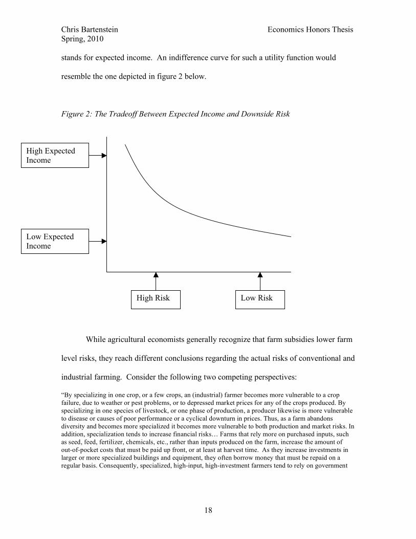
stands for expected income. An indifference curve for such a utility function would
resemble the one depicted in figure 2 below.
Figure 2: The Tradeoff Between Expected Income and Downside Risk
While agricultural economists generally recognize that farm subsidies lower farm
level risks, they reach different conclusions regarding the actual risks of conventional and
industrial farming. Consider the following two competing perspectives:
“By specializing in one crop, or a few crops, an (industrial) farmer becomes more vulnerable to a crop failure, due to weather or pest problems, or to depressed market prices for any of the crops produced. By specializing in one species of livestock, or one phase of production, a producer likewise is more vulnerable to disease or causes of poor performance or a cyclical downturn in prices. Thus, as a farm abandons diversity and becomes more specialized it becomes more vulnerable to both production and market risks. In addition, specialization tends to increase financial risks… Farms that rely more on purchased inputs, such as seed, feed, fertilizer, chemicals, etc., rather than inputs produced on the farm, increase the amount of out-of-pocket costs that must be paid up front, or at least at harvest time. As they increase investments in larger or more specialized buildings and equipment, they often borrow money that must be repaid on a regular basis. Consequently, specialized, high-input, high-investment farmers tend to rely on government
High Expected Income
Low Risk
Low Expected Income
High Risk
Chris Bartenstein Economics Honors Thesis Spring, 2010
19
commodity programs and crop insurance to protect them from production risks.”28 Vs. “With the public less willing to underwrite risk in US agriculture and with US food companies growing even more capital intensive, industrialization offers an attractive way for both the producers and food companies to hedge their risks effectively while still satisfying consumers. The large firms that control a substantial portion of the US food system are capital intense and thus must be adept at managing their risks. Staring at the consumer with one eye and at Wall Street with the other, these firms see industrialization as an effective way to manage risks that are greater and more complex. Industrialization can reduce many types of risk. It reduces supply risk by assuring a steady flow of food inputs. It reduces quality risk by guaranteeing consistent, trait specific products. It reduces financial risk by reducing the variability in input prices.”29 According to the first perspective, industrial agriculture entails greater risk than
traditional agriculture. Government safety nets, so the argument continues, raise the
willingness of farmers to shoulder the added risks of industrial agriculture, in turn
increasing the equilibrium level of agricultural industrialization in the US. According to
the second perspective, industrial agriculture lowers farmers’ overall risk. If accurate,
this perspective implies that the risk-lowering effect of federal farm subsidies has slowed
the trend toward greater aggregate agricultural industrialization among participating
farmers by making non-industrialization a safer, and therefore more viable, option. The
second perspective also implies that greater industrialization is a rational response to
lowered subsidies or expectations of soon-to-be-lowered subsidies. Parsing the
competing frames is essential to developing a solid theoretical framework relating federal
farm subsidies to risk and industrialization.
28 Ikerd, “Economics of Sustainable Farming.”
29 Dr. Mark Drabenstott, “Forces Driving Industrialization Discussion and Comment,” Industrialization of Heartland Agriculture, Agricultural Economics Miscellaneous Report,No. 176 (Conference Proceedings, July 10-11, 1995, North Dakota State University, Department of Agricultural Economics, Fargo, ND), http://ageconsearch.umn.edu/bitstream/23111/1/aem176.pdf, 23.
Chris Bartenstein Economics Honors Thesis Spring, 2010
20
In this case, the principal obstacle to consensus involves definitional ambiguity
surrounding the term “industrial” agriculture. A professor of agricultural management
addressed this point, stating, “[i]ndustrialization of agriculture has become a commonly
used and accepted descriptor of the changes occurring in agricultural production and
marketing. As is the case for many commonly accepted terms, each of us have differing
perceptions and associations with the term.” 30 Embedded in competing perspectives
relating agricultural industrialization and subsidies are different interpretations of
agricultural industrialization. In distinguishing industrial agriculture from non-industrial
agriculture, Drebenstott emphasizes distributional/structural qualities while Ikerd
emphasizes production styles. Although the structural and production-based attributes
loosely ascribed to industrial agriculture are closely interrelated,31 neither is a necessary
or sufficient condition for the other; there is no clear division in modes of production
between concentrated, vertically integrated farming operations and independently owned
farms.32 So, the currents of thought underlying the perspectives of Drebenstot and Ikerd
do not so much conflict as make distinct, although equally valid, points.
30 Dr. Stephen T. Sonka, “Forces Driving Industrialization,” Industrialization of Heartland Agriculture, Agricultural Economics Miscellaneous Report,No. 176 (Conference Proceedings, July 10-11, 1995, North Dakota State University, Department of Agricultural Economics, Fargo, ND), 13.
31 Refer to the introduction for an in-depth explanation of how structural and production based attributes of “industrial agriculture” interrelate.
32 In a May 13, 2001 New York Times Magazine article entitled “Behind the Organic Industrial Complex,” Michael Pollan identifies as a fallacy such dichotomization. Describing large, organic farming operations in California, Pollan writes: “To the eye, these farms look exactly like any other industrial farm in California -- and in fact the biggest organic operations in the state today are owned and operated by conventional mega-farms. The same farmer who is applying toxic fumigants to sterilize the soil in one field is in the next field applying compost to nurture the soil's natural fertility.” http://www.nytimes.com/2001/05/13/magazine/13ORGANIC.html?pagewanted=1, 7.
Chris Bartenstein Economics Honors Thesis Spring, 2010
21
Ceteris paribus, contractual integration of farming operations into well-capitalized
food production/distribution networks coordinated by large firms/organizations with
substantial market power and access to cheap capital, including investor wealth, may cut
down on certain types of production risk traditionally accruing to small farm managers.
The extent to which the risk advantages of upstream corporations and business entities
trickle down to farm managers depends upon the degree of integration between the two
groups. In the most extreme cases, farm managers work as salaried employees for food-
production/distribution conglomerates that hold full ownership over the land and inputs
used in production. In theory, such a manager shares the risk profile of his parent
company/organization. A more typical arrangement consists of food
processors/distributors contracting the services of farm managers who either own or rent
land. Although the universe of contractual possibilities is expansive, a common
arrangement involves a managerial pledge to sell output to a guaranteed buyer at
discounted rates in exchange for provision of inputs and farm services. This arrangement
serves to eliminate input cost risk and farm-commodity-price risk33, which are essentially
outsourced to upstream firms and their shareholders.34 Thus, to emphasize Drebenstott’s
point, industrialization may be viewed as a risk-reducing strategy from a structural
standpoint.
On the other hand, empirical research and accompanying theory indicates that the
production-based qualities commonly associated with industrial agriculture—lower crop
diversity, increased use of pesticides, heavier use of machinery etc.—are strongly 33 However, future markets for most major commodities have long served a similar purpose in the non-industrial model. 34 Contracted managers do remain exposed to the risks of rising rent costs, declining land values, unanticipated shortfalls in production, and revocation of contracts.
Chris Bartenstein Economics Honors Thesis Spring, 2010
22
correlated with higher risk.35 On an industrial farm, where only a handful of crops are
ordinarily planted each season, unfavorable growing conditions, infestations, or sharp
fluctuations in market prices can easily wipe out a full year’s revenue. Moreover, owing
to the comparative inflexibility of industrial farm operations, unanticipated input price
shifts more strongly influence profits for an industrial farm operation. Farms operating
by the principles of the alternative paradigm are theorized to be more resilient to price,
input, and crop failure risks because these farms rely less heavily on purchased inputs and
reap the benefits of a diversified portfolio of crops. Even if a crop fails or its market
value plummets, an alternative farmer will make back lost profit on other crops that
experience an especially productive growing season or that fetch an unexpectedly high
market price.
The risk reduction achieved through vertical integration is essentially unnecessary
for farmers practicing alternative styles of production. Alternative farms are not exposed
to the risks that vertical integration hedges against. On the other hand, independent
conventional farmers already practicing industrial styles of production (and probably
already receiving farm subsidies) find themselves highly vulnerable to the classes of risks
against which vertical integration protects. Therefore, small farm operations utilizing
few purchased inputs and taking advantage of high crop diversity are unlikely to consider
vertical integration with downstream processors and distributors as a risk-reducing
strategy, whereas farm operations that rely heavily on purchased inputs probably will.
35 Babcock, Bruce and Chad Hart, “Risk-Free Farming,” Iowa AG Review, Winter 2004, Vol. 10, No.1. http://www.card.iastate.edu/iowa_ag_review/winter_04/article1.aspx.
Cited in U.S. Government Accountability Office, Report to Congressional Requesters, “Farm Program Payments are an Important Factor in Landowners’ Decisions to Convert Grassland to Cropland,” Sept. 2007.
Chris Bartenstein Economics Honors Thesis Spring, 2010
23
This insight may explain the frequent concurrence of production-based and
structural attributes of IA. More importantly, it suggests a complex relationship between
government subsidies and risk-mediated industrialization. Two critical implications
follow from this line of reasoning. First, government subsidy programs probably
influence different types of farmers in different ways. Government payments may
encourage small, alternative farmers to adopt more industrial production methods if they
believe generous subsidy programs will shield them from the added risks of industrial
production. For their part, large commercial farmers may respond to payments by
delaying structural integration (structural AI) or even by disassociating with former
upstream partners.36 Second, how one measures and interprets the effects of government
payments on AI depends upon how one measures AI (i.e. whether one focuses on the
structural or the production-based components of AI).
3.3 Induced Innovation and Habits
The alternative model specifies neither divergence nor convergence in Y1 and Y2
over time. Hayami and Rutten’s theory of induced innovation provides theoretical
grounds for postulating divergence between Y1 and Y2 over time.37 According to the
“induced innovation” theory, the pace and the nature of technological development
follow prevailing factor costs. If this is indeed the case, the effect of subsidy payments
on farmer preferences may strengthen over time as technological advancement tailored to
36 These ideas are formally depicted in Appendix H.
37 Hayami and Ruttan. "Factor Prices and Technical Change in Agricultural Development: The United States and Japan.
Chris Bartenstein Economics Honors Thesis Spring, 2010
24
prevailing trends increasingly facilitates the transition toward new, industrial farming
patterns.
Moreover, induced innovation suggests that the baseline level of industrial
agriculture, the level of IA to which a farm would return if subsidy participation were
spontaneously terminated at any time (t), may diverge from the hypothetical level of IA,
the level of IA at any time (t) were subsidy programs never to have existed. Divergence
occurs when the baseline level of AI grows at a rate faster than the hypothetical level of
AI. Divergence implies that the elimination of subsidy programs would result in I.A.
levels at time t exceeding the hypothetical level of I.A. at time t had subsidy programs
never been enacted. One might hypothesize divergence on the following basis: subsidy
programs cause an increase in national levels of I.A., which entails changes in relative
demand for different agricultural factors of production and therefore the relative costs of
these factors, which induces innovation in technology conducive to more industrial forms
of agriculture, which increases baseline I.A. By this mode of reasoning, I.A. undergoes a
positive feedback loop whereby more I.A. creates a national system of agriculture more
conducive to I.A. Even if subsidy payments suddenly stopped, technological
developments stimulated by years of abnormally high IA, the residue of past payments,
would not immediately disappear.
Habit formation may also contribute to divergence between the baseline and
hypothetical levels of industrialization over time. As farmers grow accustomed to more
industrial modes of production, knowledge of less industrial methods of production may
deteriorate. Farmers who are unaware of “alternative” farming techniques will continue
producing industrially irrespective of whether the US government continues subsidizing
Chris Bartenstein Economics Honors Thesis Spring, 2010
25
farm production. Even farmers who are aware of “alternative” farming techniques may
be reticent to use them on their farms if they are more familiar and experienced with
industrial techniques.38
3.4 Modeling Theory
The graph printed below models the relationship between participation in subsidy
programs (measured by payment level) and AI for a typical farm as predicted by sections
3.1 through 3.4. In the model, “observed IA” represents actual levels of IA at different
times on a given farm. “Hypothetical IA” represents the level of IA theorized to have
prevailed on a given farm at different times under the counterfactual circumstance where
federal subsidy programs were never implemented. “Baseline AI” represents the level of
IA one would expect to observe at different times on a given farm were that farm’s
enrollment in subsidy programs suddenly terminated (which is to say, what would happen
to AI were the participation level to fall to zero).
38 There is a real economic cost associated with learning new production methods. It is rational for farmers to continue employing inefficient production techniques if the costs of learning more efficient techniques outweigh the benefits of higher efficiency.
Chris Bartenstein Economics Honors Thesis Spring, 2010
26
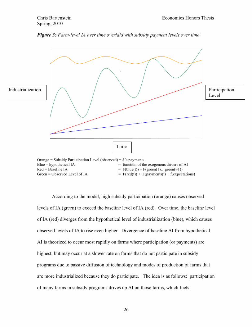
Figure 3: Farm-level IA over time overlaid with subsidy payment levels over time Orange = Subsidy Participation Level (observed) = $’s payments Blue = hypothetical IA = function of the exogenous drivers of AI Red = Baseline IA = F(blue(t)) + F(green(1)…green(t-1)) Green = Observed Level of IA = F(red(t)) + F(payments(t) + f(expectations)
According to the model, high subsidy participation (orange) causes observed
levels of IA (green) to exceed the baseline level of IA (red). Over time, the baseline level
of IA (red) diverges from the hypothetical level of industrialization (blue), which causes
observed levels of IA to rise even higher. Divergence of baseline AI from hypothetical
AI is theorized to occur most rapidly on farms where participation (or payments) are
highest, but may occur at a slower rate on farms that do not participate in subsidy
programs due to passive diffusion of technology and modes of production of farms that
are more industrialized because they do participate. The idea is as follows: participation
of many farms in subsidy programs drives up AI on those farms, which fuels
Time
Industrialization Participation Level
Chris Bartenstein Economics Honors Thesis Spring, 2010
27
technological development better suited to the industrial mode of production and brings
greater exposure among young farmers to the industrial style of production, which
eventually causes all farms, even non-participating farms, to produce more industrially
than would be the case if subsidy programs had never existed.
Figure 3 shows greater participation pushing observed AI above the hypothetical
level of AI by a relatively constant margin over time. Another possible scenario is that
individual farms’ observed level of AI begins either to converge or to diverge with the
baseline level of AI over time. Convergence means that observed IA is less sensitive to
changes in participation levels over time. Divergence implies that observed IA is more
sensitive to changes in participation levels over time. The most industrial farms are
more likely to exhibit convergence, which is to say, their levels of IA are least likely to
be affected by fluctuations in payments for two reasons. First, they already produce as
industrially as possible given existing technology (which is to say, they’ve reached a
ceiling in AI), so increases in payments couldn’t induce much further AI. Second, they
constitute the subpopulation of farmers most habituated to industrial production and most
heavily invested in industrial capital (e.g. machinery). For this reason, they may respond
only slowly, if at all, to significant drops in payments. Assuming efficient market
conditions, a farmer who refuses to adapt to macroeconomic changes will ultimately lose
his farm to a less stubborn farmer, but this process could take years if not decades,
especially if farmers value their occupation.
Despite modest uncertainty as to the ideal way in which to depict figure 3, the
important ideas to take away from the model are as follows: 1) all else equal, higher
participation in subsidy programs is theorized to correspond with higher AI over time,
Chris Bartenstein Economics Honors Thesis Spring, 2010
28
signifying that subsidy programs are responsible for higher levels of AI. 2) over the long
run, subsidy programs are theorized to push the “permanent” levels of IA (i.e. the portion
of IA not immediately influenced by current participation/payments) above the level they
would have been were it not for the subsidy program’s historical national influence on the
farm economy.
3.5 Aggregate Effects of Subsidy Programs vs. Farm Level Effects of Subsidy
Programs
That there exists an incongruity between the alternative hypothesis and the
theoretical concepts set out in Sections 3.1-3.3 deserves emphasis. The alternative
hypothesis pegs responsibility on federal farm subsidy program for higher aggregate
levels of IA in the United States, but the theory outlined in this section suggests only that
an individual farmer’s participation in subsidy programs (or anticipations thereof) may be
responsible for higher IA on his own farm, ceterus paribus. That the take-away ideas
embodied in figure 3 are correct need not imply that the alternative hypothesis is also
correct, or vice versa. All else (than participation) may not be equal on individual farms
given the aggregate effects of subsidy programs. So, the effect of subsidy programs on
aggregate IA may differ from the sum of the independent effects of individual farmers’
participation in subsidy programs.
The logical inconsistency of equating farm-level effects with aggregate effects
underlines a potential weakness in the alternative hypothesis. Alternative agriculturalists
appear to assume that if participation in subsidy programs (or anticipation thereof) is
responsible for causing farm operators to increase IA, then these programs must be
Chris Bartenstein Economics Honors Thesis Spring, 2010
29
responsible for increased levels of overall IA. The assumption is not completely without
merit. Although neither a necessary nor a sufficient condition of the alterative
hypothesis, a confirmed causal relationship between farm-level participation in subsidy
programs (or anticipation thereof) and increases in farm-level IA (i.e. support for the
theory laid out in 3.1-3.3) would suggest the strong likelihood that the alternative
hypothesis is accurate. Nonetheless, for the sake of clarity and logical consistency,
going forward, the theorized farm-level relationship between IA and subsidy programs
diagramed in 3.4 is referred to as the “weak alternative hypothesis” (WAH) to distinguish
it from its analogue, the “strong alternative hypothesis” (SAH). The WAH proposes the
following: ceterus paribus, participation in subsidy programs and the anticipation thereof
cause higher levels of IA.
4 Empirical Analysis
Since Y2 represents a hypothetical value that cannot be observed directly,39
whether the difference between Y2 and Y1, or X, is negative or positive cannot be
observed. In order to disprove the alternative hypothesis, that farm subsidy programs
push equilibrium aggregate industrialization beyond its hypothetical, or non-interference
level, one would need to provide statistically significant evidence that X has not
consistently exceeded zero in recent history.40
39 Not to mention, agricultural industrialization describes a group of abstract and related concepts, so quantifying its values essentially amounts to an exercise in estimation even where its characteristic manifestations can be observed. 40 Proponents of the alternative paradigm are concerned with the current effects of subsidies. Since subsidy programs have been revamped in recent decades, only X values spanning the last ten or fifteen years are remotely indicative of current X values. So X would need to be estimated for recent points in time.
Chris Bartenstein Economics Honors Thesis Spring, 2010
30
Unfortunately, there does not appear to be a feasible way to estimate the direction
of X (whether it is positive or negative) at a given time. Trying to predict current values
for Y2 (in order to find X) on the basis of deep historical data is a fruitless venture. Farm
subsidies have existed since the Great Depression, and the US economy of the 1920’s
differed too much from today’s economy for forward extrapolation of this sort to be
meaningful. Regressing time series measures of aggregate AI on time series measures of
aggregate subsidy program participation in the US to estimate the independent effects of
federal subsidization (for the sake of reverse engineering Y2) also fails to produce
meaningful estimates of X. Given the timeframe over which changes in industrialization
are theorized to influence I.A., such an analysis would require data spanning many
decades to achieve statistical significance. Over a time horizon measured in decades, the
effects of federal subsidization no doubt interact in countless ways with autonomous
historical developments (external factors) to influence industrialization in unpredictable
ways. A given level of subsidization undoubtedly has influenced IA in different ways at
different times, ceteris paribus, which means that the historic effects of participation in
programs are not necessarily identical to the current effects of participation.41 Moreover,
federal subsidy programs have changed significantly over time. Controlling for all
relevant, variable factors (and interaction terms) and setting an objective measure of AI
over historical time is impractical,42 and running a time series regression of this nature
without effective controls and measurement schematics would yield irrelevant results.
41 Though, most alternative movement proponents would suggest the effect has been uniformly positive over time. 42 Such an approach suffers auto-correlation and data availability problems.
Chris Bartenstein Economics Honors Thesis Spring, 2010
31
A more reasonable strategy for analyzing the current relationship between IA and
farm subsidization is to focus not on estimating the influence of federal subsidization on
aggregate IA over many periods, but on estimating how subsidy programs affect many
subdivisions of the US farm economy over one period. The regression model defined
above avoids the complications of time series regressions by focusing exclusively on the
effects of changes in participation on AI in one (recent) period. Focusing on just one
period confers a major advantage: it enables the researcher to circumvent the problem of
non-identical historical effects of subsidy programs and control variables. On the other
hand, because such a model deals with sub-aggregate farm data, it fails to capture the
aggregate/systemic effects of subsidy programs (those effects which influence all farmers
approximately equally). So, pursuing such a strategy serves as a direct challenge/test of
the WAH, but only provides speculative, though useful, evidence regarding the accuracy
of the SAH.
4.1 Modeling Regressions
A fundamental problem with judging the validity of the alternative hypothesis
based on the extent to which changes in IA correlate with changes in participation at an
earlier time is that the body of theory on which the “alternative hypothesis” rests does not
necessarily predict increases in A.I. following measurable increases in participation or
payment rates. Changes in industrialization mediated by risk (described in 3.3) logically
should succeed actual changes in participation or levels of subsidy support, but changes
in industrialization mediated by the “subsidy straitjacket” (described in 3.2) may succeed
realized changes in participation or realized changes in levels of subsidy support.
Chris Bartenstein Economics Honors Thesis Spring, 2010
32
Modern farmers wishing to reap the benefits of payment programs may feel obliged to
subject themselves to the “subsidy straitjacket” prior to changes in actual subsidy
receipts. The fact that the most recent three farm bills have stipulated fixed payments
pegged to crop statistics for the years immediately preceding new bills explains this
behavior.43 As discussed in section 3.2, theory indicates that farmers may even revert to
less industrial modes of production subsequent to acquiring entitlements to fixed
payments.44 Therefore, expectations about future payment programs presumably play at
least as important a role in influencing farm-level industrial agriculture as do realized
changes in subsidy support.
The complexity of the relationship between subsidy programs and AI warrants the
use of multiple regressions as a means of examining the WAH. The WAH postulates two
operant chains of causality that link farm subsidy programs with increases in observed
AI. These two relationships can be summarized in the following way: 45
1) Farm Subsidy Programs ∆ participation non anticipation based ∆ AI 2) Farm Subsidy Programs anticipation based ∆ AI ∆ participation According to this model, subsidy programs are ultimately responsible for changes in AI
under both causal pathways. However, there is no way in which to capture the influence
43 See Appendix B.
44 If the risk-mediated effects of subsidy payments are negative, neutral, or only weakly positive (it was theorized the effect could go either way, depending upon how IA is measured), and payment programs do not match farmers expectations, increases in government payments may correlate with decreases in IA on account of changed expectations (irrespective of the actual effects of changes in payments) because expectations of the present value of future participation are modified down. Expectations cannot be controlled since they cannot be measured.
45 An in-depth analysis of the hypothesized relationship between government programs, IA, and participation in subsidy programs (according to the WAH) is laid out in Appendix D.
Chris Bartenstein Economics Honors Thesis Spring, 2010
33
of the simple existence of farm subsidy programs on changes in AI by way of statistical
analysis since the existence of subsidy programs is a constant across space and time.46
One is limited to examining the legitimacy of these proposed causal pathways by
working with proxy data for each of the remaining two variables (∆ AI and ∆
participation). If causal pathway 1 is correct, changes in proxies for participation over a
given period should correlate (causally) with changes in proxies AI over a succeeding
period. If causal pathway 2 is correct, changes in proxies for AI over a given period
should correlate (causally) with changes in proxies for participation over a succeeding
period.47 An appropriately controlled regression model can be used to test each of these
relationships.
Since the WAH theorizes that the effects of industrialization occur at the level of
the individual farm, data for individual farms would be ideal for use in these regressions.
Unfortunately, data on payments to individual farms or individual farm operators and
data on indicators for IA on individual farms or attributable to individual farm operators
are not available to the general public. The lowest unit of analysis for which data falls
within the public domain is the county.48 Consequently, county level data are used in
place of farm level data in the regression models.
46 In other words, there is no variance in this variable.
47 To simply regress levels of IA on levels of participation and vice versa would be to invite serious endogeneity/selection-bias problems. Actual levels of participation and IA depend too much upon historical factors that cannot be controlled with available data. Appendix G provides a detailed explanation of the sorts of problematic biases such a regression model would potentially introduce. 48 The USDA collects information from individual farm operations every five years when it conducts the agricultural census, but publishes composite statistics representing entire counties and states. The USDA cannot disclose data that uniquely identifies attributes of individual farm operations. So, although farm-level data exist, they cannot be legally obtained. The USDA does use farm-level data in its internal studies, and, for a fee, appears to provide a service that enables third party researchers to crunch primary, farm-level data without actually seeing the individual
Chris Bartenstein Economics Honors Thesis Spring, 2010
34
Running a regression using county data risks biasing the results if farm operations
are systematically grouped according to a nonrandom metric. It seems reasonable to treat
farm operations as randomly distributed across counties, especially if basic demographic
factors are controlled. So, the “∆ participation” coefficient for a county level regression
is considered an unbiased estimator of the “∆ participation” coefficient for a farm
operation level regression, and the same is true of the ∆ IA coefficient in regression 2.
So, results of a county level regression may be used to analyze the weak and strong
alternative hypotheses in the same way as results from a farm-operation level regression
would be.
4.2 Two Additional Assumptions
1) As with any linear regression, our model imposes a linear relationship between the
dependent and the independent variables. The true nature of the functional relationship
between IA and subsidy program participation at the farm level is unknown, and may not
conform perfectly to the linear assumption. However, as long as the relationships
between the dependent and the independent variables are monotonic in either regression,
the sign of the revealed coefficient will accurately construe whether the two variables are
negatively or positively correlated, irrespective of the mathematical relationship between
the two.49
data points. The value of this service to my regression did not seem to justify its costs (in terms of time and money). 49 If the linear assumption is extremely far off the mark, we could end up with meaningless significance levels, but it seems highly improbable that this would be the case. The constant marginal effect assumption makes sense in light of an underlying premise of section 3 theory: that all farmers behave in similar and predictable ways.
Chris Bartenstein Economics Honors Thesis Spring, 2010
35
2) Given the likelihood that the true marginal effects of changes in the independent
variables on the dependent variables differ between different subpopulations of farmers,50
we must assume that variance in the independent variables is randomly distributed across
the farm population if we would like to treat the revealed coefficient for each independent
as reflective of the average farmer’s predicted behavior. Otherwise, we wind up
attributing the behaviors of a unique sub-population of farmers to that of the entire US
farm economy, painting a skewed picture of reality. The criterion of random selection is
almost certainly not met.51 The sub-population of farmers responsible for the majority of
measurable fluctuations in IA and subsidy program participation probably does reflect the
population of farmers as a whole. In fact, if causal chains 1 and 2 are both accurate, we
know that IA and participation influence each other over the long run, and so if either one
is non-randomly distributed, neither one is. This is not a critical flaw, but an issue that
deserves recognition.
4.3 Setting Appropriate Lags
Given long-run bidirectional causality between IA and participation in subsidy
programs, it is necessary to lag the first differencing period of the independent variable
on the first differencing period of the dependent variable so that the effects ascribed to
the independent variable are not contaminated by bidirectional causality. Logic warrants
that an event cannot be affected by a succeeding event, so a lag should resolve the reverse
50 Level of participation in government probably does not influence all farmers’ decisions in similar ways.
51 For example, farmland being registered for and withdrawn from subsidy programs is likely to differ in key respects from farmland that remains registered or never is registered for subsidy support, and farmers choosing to register or withdraw land from subsidy programs are likely to differ from each other and from farmers who leave farmland registered.
Chris Bartenstein Economics Honors Thesis Spring, 2010
36
causality problem. The best way in which to set a lag in a given regression depends
upon the following two questions: when are changes in the independent variable most
likely to influence changes in the dependent variable? And, for which periods are data
available?
For better or for worse, data limitations severely constrain the number of ways in
which an individual can design lagged regressions of county participation on county AI
and vice versa. Agricultural census data are only available electronically for the most
recent three censuses: the1997 Census, the 2002 Census, and the 2008 Census.
For the purposes of my experiment, the number of electronically available
agricultural censuses and their timing were fortuitous. These three snapshots in time
yield two distinct periods over which to calculate first differences. The 1997 census was
published one year after the 1996 farm bill was passed into law, the 2002 census was
published in the very same ear as the 2002 farm bill was passed into law, and the 2007
farm census was published shortly before the 2008 farm bill was passed. Having two
periods enables lags for regressions testing causal pathway 1 and 2, and that periods 1
and 2 collectively span the life of two distinct farm bills fulfills a necessary data
requirement for testing causal pathway 1.
Prior to passage of the 2002 farm bill, there were effectively no opportunities for
farmers to increase their level of participation in subsidy programs by altering their level
of AI. During these years payments were tied to production statistics covering years
prior to 1996. Meanwhile, there would have been no reason for individuals who
decreased AI to request lower payments over the remainder of the life of the 1996 bill.
Although farmers could not realistically have parlayed changes in AI into changes in
Chris Bartenstein Economics Honors Thesis Spring, 2010
37
participation until 2002, between 1996 and 2002, many farmers are expected to have
industrialized in anticipation that doing so would enable them to capture higher subsidy
payments after the 2002 farm bill was passed (which would increase their expected
income and cut down on risk). Conversely, many farmers who shared in the impression
that subsidy payments would soon be phased out may have chosen to de-industrialize
production; absent subsidy payments, these farmers were not willing to underwrite the
risks of industrial agriculture. Other farmers may have undergone anticipatory decreases
in AI due to the impression that expected future subsidy payoffs no longer justified the
opportunity cost of sustaining modes of production assumed necessary to continue
receiving payments in the future.
Presumably, most farmers hold reasonable expectations and so sustain new levels
of AI into subsequent periods in hopes of continuing to receive payments under later
subsidy programs. However, those farmers whose expectations turn out to misalign with
future preferences are expected to revert to IA levels exhibited prior to forming mistaken
expectations. 52 Participation is also expected fall to baseline levels under this scenario,
although perhaps not as immediately since payments depend more on past production
methods than present production methods. Due to the ability of farmers to update
expectations as history unfolds, general overestimation or underestimation biases across
all county observations over a given period in time could influence the way in which
changes in IA correlate with changes in participation at different future points in time53
52 This is depicted in Appendix E 53 This concept is explored in greater detail in the regression analysis.
Chris Bartenstein Economics Honors Thesis Spring, 2010
38
That anticipation-based changes in IA can only influence changes in payments
subsequent to a change in farm bills implies that changes in AI between 1996 and 2001
intended to enable changes in future participation should not have influenced changes in
participation over these same five years. Period 1 (spanning the time between 1997
census observations and 2002 census observations) captures five years over which time
accumulating changes in AI from prior to 2002 could not have influenced participation
(1996-2001), and one growing season, 2002, over which they could. Period 2 captures an
additional five years over which accumulated changes in IA from prior to 2002 could
have influenced farmer participation. Changes in IA in period one can be regressed on
changes in participation in period 2 as a test of WAH causal pathway 2 without running
the risk of reverse causality entering into the picture. However, if most of the changes in
participation caused by previous changes in IA occur immediately after passage of the
2002 farm bill, such a lagged regression may not have statistical significance. For this
reason, both a lagged and a non-lagged regression are used to test causal pathway 2 in
this thesis. The non-lagged regression uses period one changes in participation (which
amount to 2002 changes) on period one changes in IA (which presumably occur all
throughout 2002). The prospect of reverse-causality endogeneity enters into the picture
for 2002 using the non-lagged model, but as long as the effects of changes in
participation on changes in IA do not occur rapidly, the one year overlap of changes in IA
and changes in participation caused by changes in IA shouldn’t fundamentally distort the
true effect of changes in IA on increases in participation in 2002.
Selecting an appropriate lag structure for the regression examining how changes
in participation influence IA (causal pathway 1) is less difficult. Unlike the effect of
Chris Bartenstein Economics Honors Thesis Spring, 2010
39
changes in IA on changes in participation, the effect of changes in participation on IA is
theorized to occur continuously and gradually with no breaks in effects between farm
bills as changes in income, wealth, and expected income slowly modify a farmer’s risk
profile. So, measurement periods need not correspond with changes in farm bills: one
lagged regression model should suffice. Its difficult to predict the precise timeframe over
which changes in participation might lead to changes in IA, but the existence of two
complete, contiguous periods, permits only one viable lagged regression model: a
regression of changes in participation over period 1 on changes in IA in period 2. So
long as some of the effect of changes in participation between 1996 and 2002 on changes
in IA occurs between 2002 and 2007, this model should capture the general direction of
the overall effect.
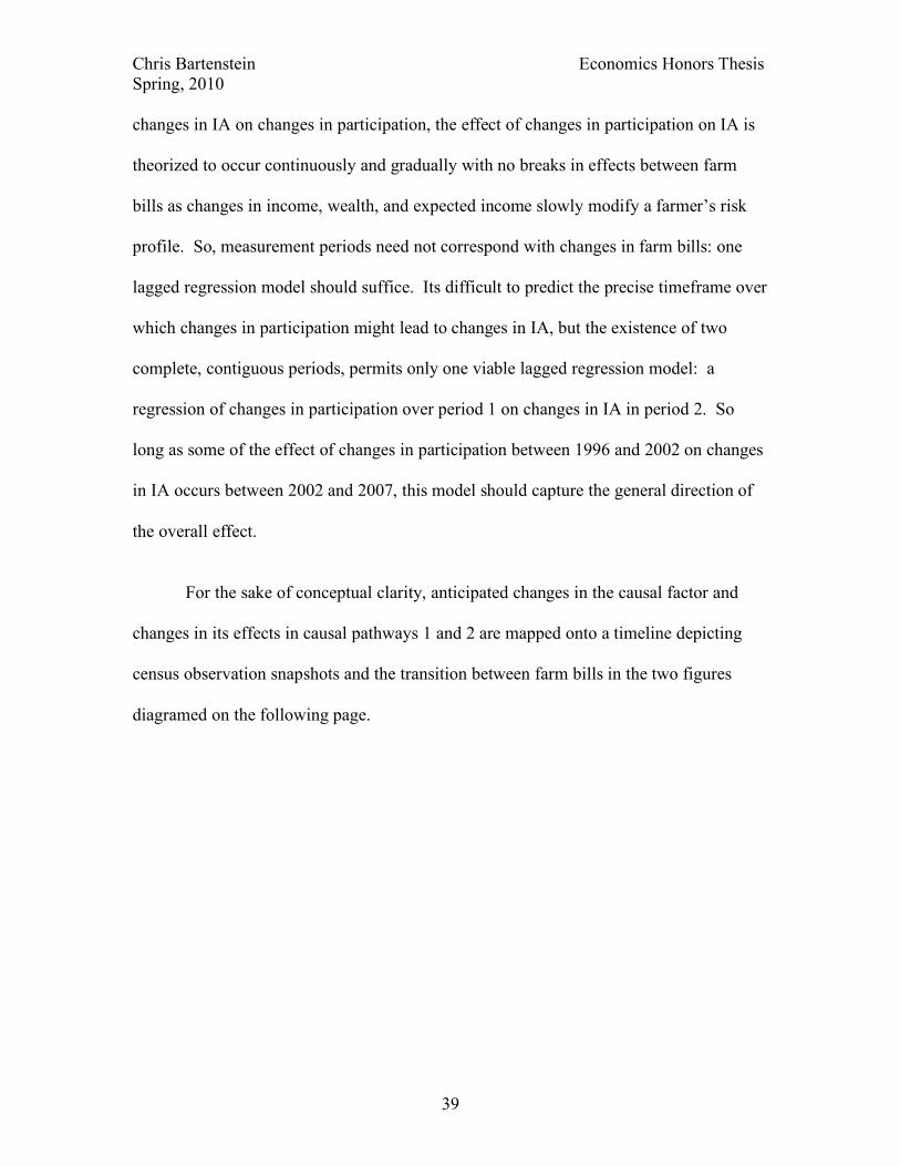
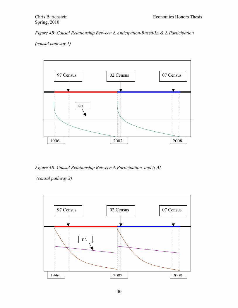
For the sake of conceptual clarity, anticipated changes in the causal factor and
changes in its effects in causal pathways 1 and 2 are mapped onto a timeline depicting
census observation snapshots and the transition between farm bills in the two figures
diagramed on the following page.
Chris Bartenstein Economics Honors Thesis Spring, 2010
40
Figure 4B: Causal Relationship Between ∆ Anticipation-Based-IA & ∆ Participation
(causal pathway 1)
Figure 4B: Causal Relationship Between ∆ Participation and ∆ AI
(causal pathway 2)
1996 2002 2008
97 Census 02 Census 07 Census
1996 2002 2008
97 Census 02 Census 07 Census
E2
E3
Chris Bartenstein Economics Honors Thesis Spring, 2010
41
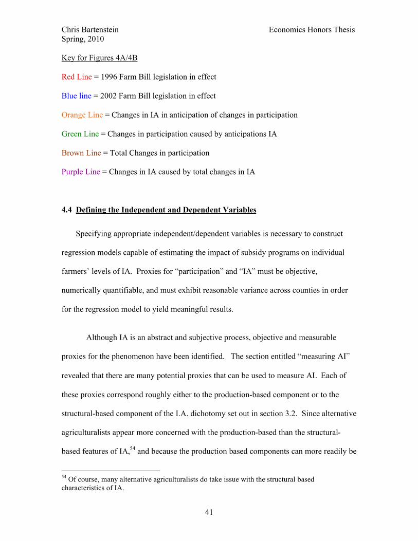
Key for Figures 4A/4B
Red Line = 1996 Farm Bill legislation in effect
Blue line = 2002 Farm Bill legislation in effect
Orange Line = Changes in IA in anticipation of changes in participation
Green Line = Changes in participation caused by anticipations IA
Brown Line = Total Changes in participation
Purple Line = Changes in IA caused by total changes in IA
4.4 Defining the Independent and Dependent Variables
Specifying appropriate independent/dependent variables is necessary to construct
regression models capable of estimating the impact of subsidy programs on individual
farmers’ levels of IA. Proxies for “participation” and “IA” must be objective,
numerically quantifiable, and must exhibit reasonable variance across counties in order
for the regression model to yield meaningful results.
Although IA is an abstract and subjective process, objective and measurable
proxies for the phenomenon have been identified. The section entitled “measuring AI”
revealed that there are many potential proxies that can be used to measure AI. Each of
these proxies correspond roughly either to the production-based component or to the
structural-based component of the I.A. dichotomy set out in section 3.2. Since alternative
agriculturalists appear more concerned with the production-based than the structural-
based features of IA,54 and because the production based components can more readily be
54 Of course, many alternative agriculturalists do take issue with the structural based characteristics of IA.
Chris Bartenstein Economics Honors Thesis Spring, 2010
42
observed/quantified, two separate “production-based” proxies of IA, fertilizer expense55
and chemical expense,56 serve as the dependent variable in the regression analysis. As
discussed in 3.2, production based proxies for AI industrialization are more likely to
increase with increases in participation than are “structural” proxies. So the regression of
IA on subsidy payments is more likely to yield a positive coefficient on the subsidy
payments variable than would be the case were structural-based measurement s of AI
used.
Subsidy payments qualify as an ideal proxy for level of participation in subsidy
programs. In fact, theory from section 3 suggests that payments function as one of the
two causal mechanisms by which increased participation may increase IA (insofar as they
alter perception of risk). The second mechanism by which theory predicts participation
influences IA is the constraints placed on farmers when they elect to register land for
subsidy payments (or the constraints which they place on themselves in anticipation of
future participations). Although the second mechanism is causally unrelated to actual
levels of payments, the extent to which a given farm operation participates in subsidy
programs, and therefore finds itself constrained by the standards of these programs,
certainly scales with level of payments (more payments = more land registered under
more programs = more restrictions placed on larger portions of growing areas). So to
55 Dollars spent on fertilizer yielded the highest average correlation with the other proxies for AI, so this proxy is used for the regression.
56 “[Chemical] expenses include the cost of all insecticides, herbicides, fungicides, and other pesticides, including the cost of custom application. Data exclude commercial fertilizer purchased.” Agricultural Census 2002.
Chris Bartenstein Economics Honors Thesis Spring, 2010
43
reemphasize, payments directly measure the first mechanism and indirectly, though
accurately, measure the second mechanism linking participation with IA.
Payment levels may uniformly rise or fall as a result of legislative or economic
shocks, but the relative levels of payments should still correspond to a farmer’s level of
participation in subsidy programs in relation to the level of participation of other farmers.
There is noise in the payments proxy. One would ideally prefer a proxy that only
captured payments stemming from federal commodity programs, as these are the
programs predicted by alternative agriculturalists to increase IA. Unfortunately, a portion
of the variation in the payments variable is attributable to differences in subsidy
payments stemming from non-commodity programs or temporary legislation.
Disaggregated Conservation Reserve payment data are publicly available and so have
been controlled (by subtracting conservation reserve payments from net government
payments), but other non-commodity program government payments (e.g. emergency
payments) are not available in disaggregated form, and so contaminate our participation
proxy. If the noise is randomly distributed across the sample, it merely creates a
downward bias in beta coefficients for participation and lowers its significance. If not,
endogeneity results. I do not anticipate this being a major problem because in the years
of measurement (1997, 2002, and 2007) most payments were attributable to commodity
programs (refer to appendix B).
Chris Bartenstein Economics Honors Thesis Spring, 2010
44
4.5 Controls
1) Regression toward the Mean and Base Level Controls
Studies have shown preexisting levels of industrialization to be negatively
correlated with rates of industrialization. To re-invoke the MacCannell study:
“Correlations between the nine variables and their rates of change between 1970 and 1980 are generally significant and negative, suggesting that the least industrialized of the counties underwent the most rapid change in percentage terms. MacCannell suggests this trend would lead to a more uniform industrial agricultural system throughout the area.”57
In other words, more industrialized counties generally continue to industrialize at a
slower pace than less industrialized counties. Preexisting industrialization should
therefore be used as a control in regressions of changes in IA on changes in payments.
This example provides a clear example of just one of many ways in which base levels of
IA and base levels of participation could potentially explain much of the variation in
future changes in these same variables. So, base level variables (1997 census values) are
used as controls in each regression.
2) Region, Factor Cost, and Farm Use Data
One cannot overemphasize the importance of controlling for sources of change in
participation causally unrelated to changes in IA in the first model and of controlling for
sources of change in IA causally unrelated to changes in participation in the second
model. Changes in IA and in participation no doubt correlate with all order of farm-
economy factors that independently influence the respective dependent variable in the
regressions. Controlling for the most obvious suspects (e.g. factor costs, demographic
57 Dean MacCannell, “Industrial Agriculture and Rural Community Degradation.”
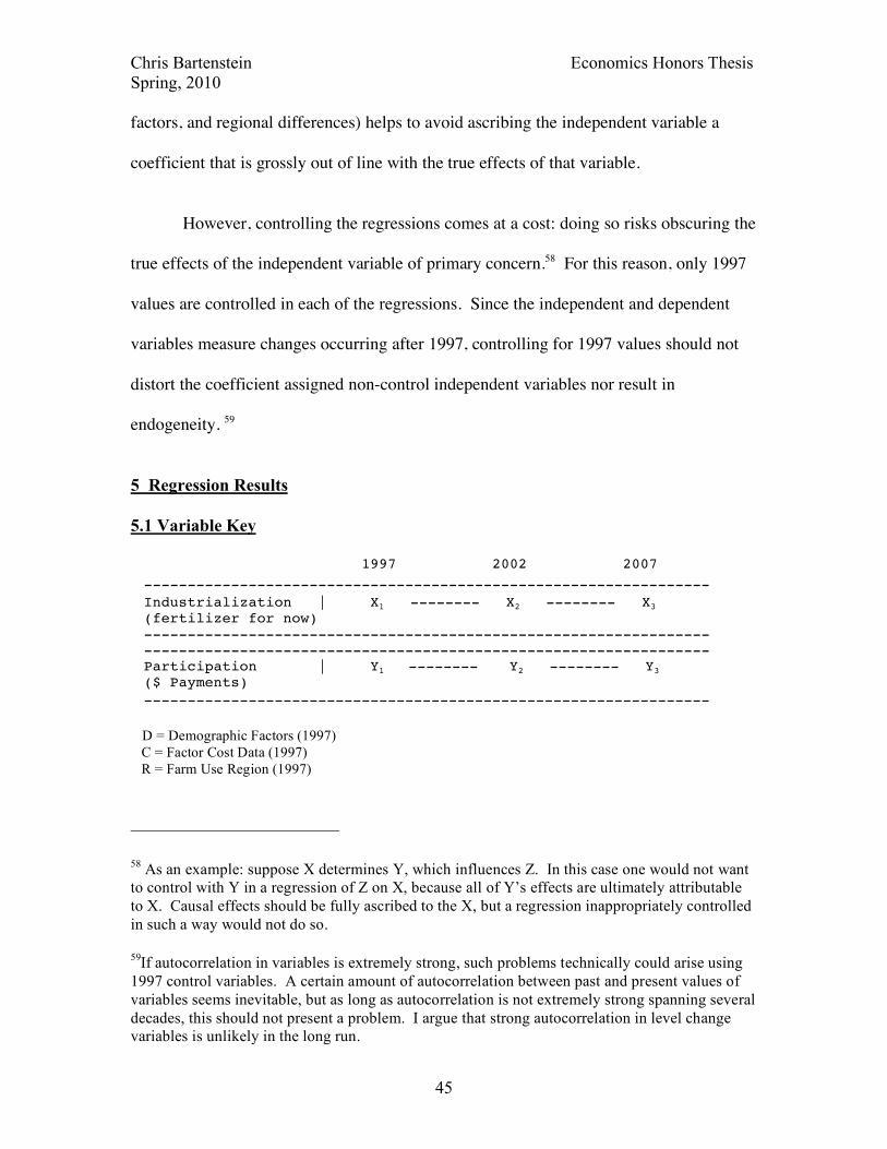
Chris Bartenstein Economics Honors Thesis Spring, 2010
45
factors, and regional differences) helps to avoid ascribing the independent variable a
coefficient that is grossly out of line with the true effects of that variable.
However, controlling the regressions comes at a cost: doing so risks obscuring the
true effects of the independent variable of primary concern.58 For this reason, only 1997
values are controlled in each of the regressions. Since the independent and dependent
variables measure changes occurring after 1997, controlling for 1997 values should not
distort the coefficient assigned non-control independent variables nor result in
endogeneity. 59
5 Regression Results
5.1 Variable Key
1997 2002 2007 ----------------------------------------------------------------- Industrialization | X1 -------- X2 -------- X3
(fertilizer for now) ----------------------------------------------------------------- ----------------------------------------------------------------- Participation | Y1 -------- Y2 -------- Y3 ($ Payments) -----------------------------------------------------------------
D = Demographic Factors (1997) C = Factor Cost Data (1997) R = Farm Use Region (1997)
58 As an example: suppose X determines Y, which influences Z. In this case one would not want to control with Y in a regression of Z on X, because all of Y’s effects are ultimately attributable to X. Causal effects should be fully ascribed to the X, but a regression inappropriately controlled in such a way would not do so.
59If autocorrelation in variables is extremely strong, such problems technically could arise using 1997 control variables. A certain amount of autocorrelation between past and present values of variables seems inevitable, but as long as autocorrelation is not extremely strong spanning several decades, this should not present a problem. I argue that strong autocorrelation in level change variables is unlikely in the long run.
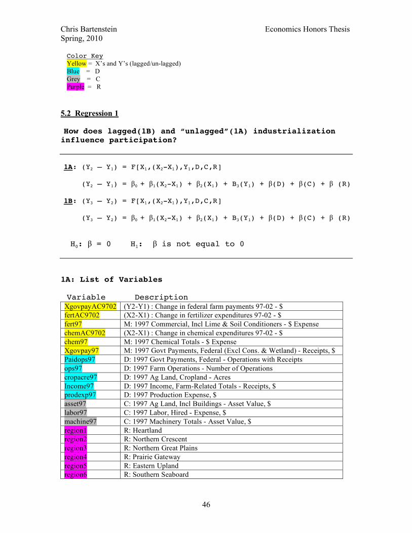
Chris Bartenstein Economics Honors Thesis Spring, 2010
46
Color Key Yellow = X’s and Y’s (lagged/un-lagged) Blue = D Grey = C Purple = R
5.2 Regression 1 How does lagged(1B) and “unlagged”(1A) industrialization influence participation? 1A: (Y2 – Y1) = F[X1,(X2-X1),Y1,D,C,R] (Y2 – Y1) = β0 + β1(X2-X1) + β2(X1) + B3(Y1) + β(D) + β(C) + β (R) 1B: (Y3 – Y2) = F[X1,(X2-X1),Y1,D,C,R] (Y3 – Y2) = β0 + β1(X2-X1) + β2(X1) + B3(Y1) + β(D) + β(C) + β (R) H0: β = 0 H1: β is not equal to 0
1A: List of Variables Variable Description
XgovpayAC9702 (Y2-Y1) : Change in federal farm payments 97-02 - $ fertAC9702 (X2-X1) : Change in fertilizer expenditures 97-02 - $ fert97 M: 1997 Commercial, Incl Lime & Soil Conditioners - $ Expense chemAC9702 (X2-X1) : Change in chemical expenditures 97-02 - $ chem97 M: 1997 Chemical Totals - $ Expense Xgovpay97 M: 1997 Govt Payments, Federal (Excl Cons. & Wetland) - Receipts, $ Paidops97 D: 1997 Govt Payments, Federal - Operations with Receipts ops97 D: 1997 Farm Operations - Number of Operations cropacre97 D: 1997 Ag Land, Cropland - Acres Income97 D: 1997 Income, Farm-Related Totals - Receipts, $ prodexp97 D: 1997 Production Expense, $ asset97 C: 1997 Ag Land, Incl Buildings - Asset Value, $ labor97 C: 1997 Labor, Hired - Expense, $ machine97 C: 1997 Machinery Totals - Asset Value, $ region1 R: Heartland region2 R: Northern Crescent region3 R: Northern Great Plains region4 R: Prairie Gateway region5 R: Eastern Upland region6 R: Southern Seaboard
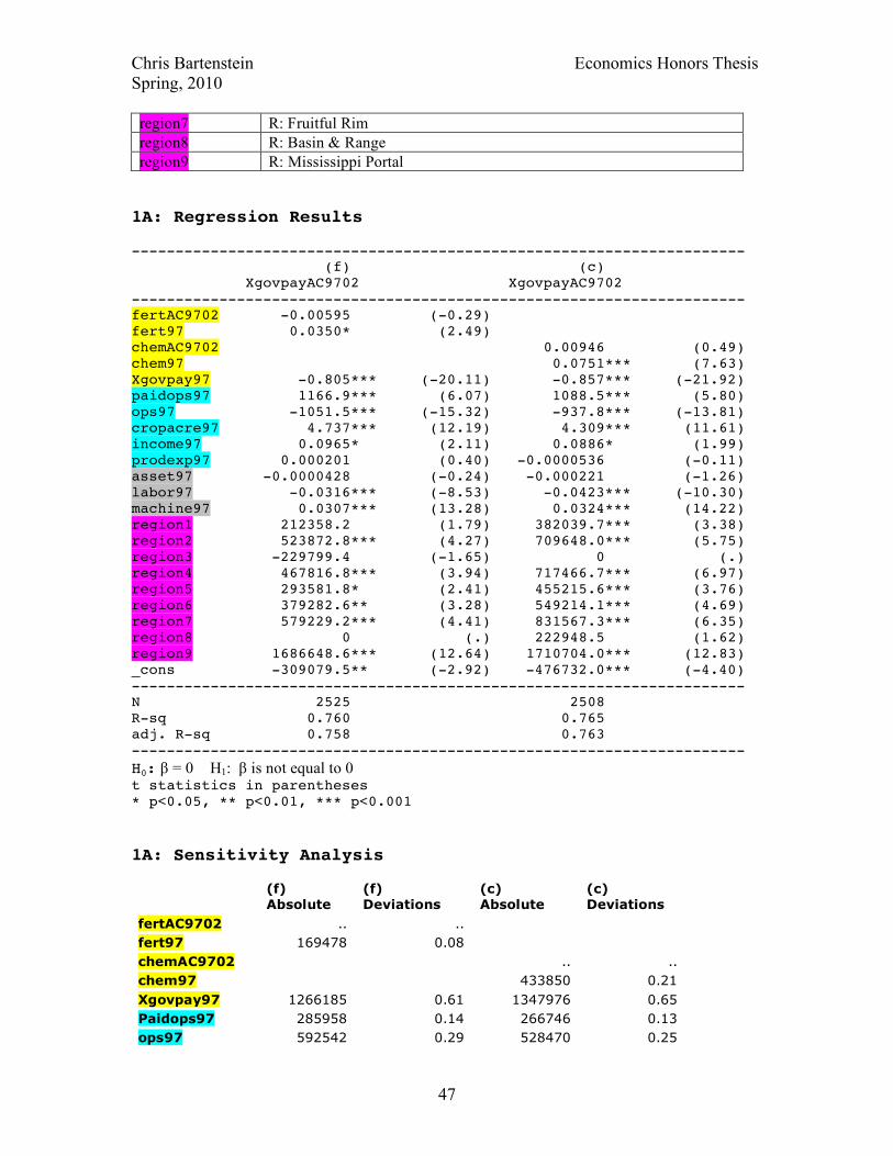
Chris Bartenstein Economics Honors Thesis Spring, 2010
47
region7 R: Fruitful Rim region8 R: Basin & Range region9 R: Mississippi Portal
1A: Regression Results ---------------------------------------------------------------------- (f) (c) XgovpayAC9702 XgovpayAC9702 ---------------------------------------------------------------------- fertAC9702 -0.00595 (-0.29) fert97 0.0350* (2.49) chemAC9702 0.00946 (0.49) chem97 0.0751*** (7.63) Xgovpay97 -0.805*** (-20.11) -0.857*** (-21.92) paidops97 1166.9*** (6.07) 1088.5*** (5.80) ops97 -1051.5*** (-15.32) -937.8*** (-13.81) cropacre97 4.737*** (12.19) 4.309*** (11.61) income97 0.0965* (2.11) 0.0886* (1.99) prodexp97 0.000201 (0.40) -0.0000536 (-0.11) asset97 -0.0000428 (-0.24) -0.000221 (-1.26) labor97 -0.0316*** (-8.53) -0.0423*** (-10.30) machine97 0.0307*** (13.28) 0.0324*** (14.22) region1 212358.2 (1.79) 382039.7*** (3.38) region2 523872.8*** (4.27) 709648.0*** (5.75) region3 -229799.4 (-1.65) 0 (.) region4 467816.8*** (3.94) 717466.7*** (6.97) region5 293581.8* (2.41) 455215.6*** (3.76) region6 379282.6** (3.28) 549214.1*** (4.69) region7 579229.2*** (4.41) 831567.3*** (6.35) region8 0 (.) 222948.5 (1.62) region9 1686648.6*** (12.64) 1710704.0*** (12.83) _cons -309079.5** (-2.92) -476732.0*** (-4.40) ---------------------------------------------------------------------- N 2525 2508 R-sq 0.760 0.765 adj. R-sq 0.758 0.763 ---------------------------------------------------------------------- H0: β = 0 H1: β is not equal to 0 t statistics in parentheses * p<0.05, ** p<0.01, *** p<0.001 1A: Sensitivity Analysis
(f) Absolute
(f) Deviations
(c) Absolute
(c) Deviations
fertAC9702 .. .. fert97 169478 0.08 chemAC9702 .. .. chem97 433850 0.21 Xgovpay97 1266185 0.61 1347976 0.65 Paidops97 285958 0.14 266746 0.13 ops97 592542 0.29 528470 0.25
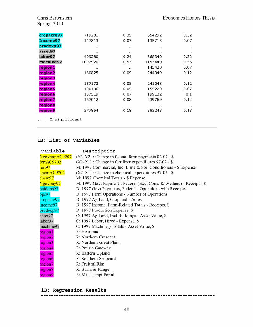
Chris Bartenstein Economics Honors Thesis Spring, 2010
48
cropacre97 719281 0.35 654292 0.32 Income97 147813 0.07 135713 0.07 prodexp97 .. .. .. .. asset97 .. .. .. .. labor97 499280 0.24 668340 0.32 machine97 1092920 0.53 1153440 0.56 region1 .. .. 145420 0.07 region2 180825 0.09 244949 0.12 region3 .. .. region4 157173 0.08 241048 0.12 region5 100106 0.05 155220 0.07 region6 137519 0.07 199132 0.1 region7 167012 0.08 239769 0.12 region8 .. .. region9 377854 0.18 383243 0.18
.. = Insignificant
1B: List of Variables Variable Description
XgovpayAC0207 (Y3-Y2) : Change in federal farm payments 02-07 - $ fertAC9702 (X2-X1) : Change in fertilizer expenditures 97-02 - $ fert97 M: 1997 Commercial, Incl Lime & Soil Conditioners - $ Expense chemAC9702 (X2-X1) : Change in chemical expenditures 97-02 - $ chem97 M: 1997 Chemical Totals - $ Expense Xgovpay97 M: 1997 Govt Payments, Federal (Excl Cons. & Wetland) - Receipts, $ paidops97 D: 1997 Govt Payments, Federal - Operations with Receipts ops97 D: 1997 Farm Operations - Number of Operations cropacre97 D: 1997 Ag Land, Cropland - Acres income97 D: 1997 Income, Farm-Related Totals - Receipts, $ prodexp97 D: 1997 Production Expense, $ asset97 C: 1997 Ag Land, Incl Buildings - Asset Value, $ labor97 C: 1997 Labor, Hired - Expense, $ machine97 C: 1997 Machinery Totals - Asset Value, $ region1 R: Heartland region2 R: Northern Crescent region3 R: Northern Great Plains region4 R: Prairie Gateway region5 R: Eastern Upland region6 R: Southern Seaboard region7 R: Fruitful Rim region8 R: Basin & Range region9 R: Mississippi Portal
1B: Regression Results ----------------------------------------------------------------------
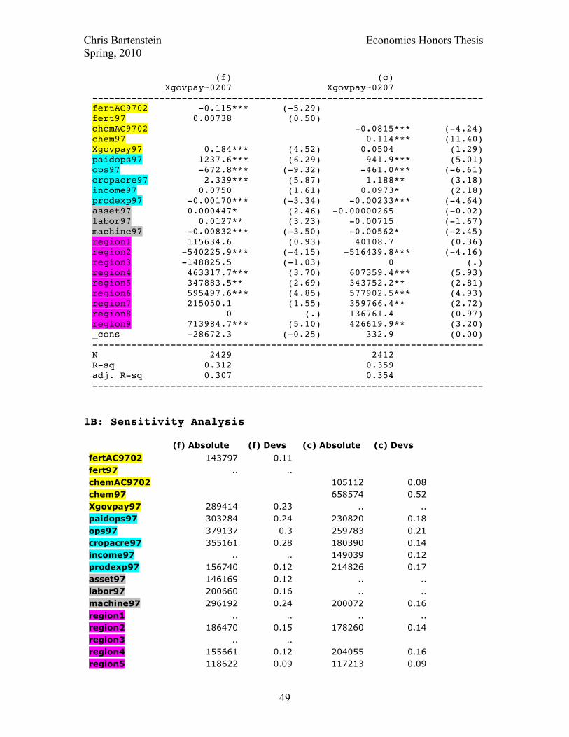
Chris Bartenstein Economics Honors Thesis Spring, 2010
49
(f) (c) Xgovpay~0207 Xgovpay~0207 ---------------------------------------------------------------------- fertAC9702 -0.115*** (-5.29) fert97 0.00738 (0.50) chemAC9702 -0.0815*** (-4.24) chem97 0.114*** (11.40) Xgovpay97 0.184*** (4.52) 0.0504 (1.29) paidops97 1237.6*** (6.29) 941.9*** (5.01) ops97 -672.8*** (-9.32) -461.0*** (-6.61) cropacre97 2.339*** (5.87) 1.188** (3.18) income97 0.0750 (1.61) 0.0973* (2.18) prodexp97 -0.00170*** (-3.34) -0.00233*** (-4.64) asset97 0.000447* (2.46) -0.00000265 (-0.02) labor97 0.0127** (3.23) -0.00715 (-1.67) machine97 -0.00832*** (-3.50) -0.00562* (-2.45) region1 115634.6 (0.93) 40108.7 (0.36) region2 -540225.9*** (-4.15) -516439.8*** (-4.16) region3 -148825.5 (-1.03) 0 (.) region4 463317.7*** (3.70) 607359.4*** (5.93) region5 347883.5** (2.69) 343752.2** (2.81) region6 595497.6*** (4.85) 577902.5*** (4.93) region7 215050.1 (1.55) 359766.4** (2.72) region8 0 (.) 136761.4 (0.97) region9 713984.7*** (5.10) 426619.9** (3.20) _cons -28672.3 (-0.25) 332.9 (0.00) ---------------------------------------------------------------------- N 2429 2412 R-sq 0.312 0.359 adj. R-sq 0.307 0.354 ----------------------------------------------------------------------
1B: Sensitivity Analysis
(f) Absolute (f) Devs (c) Absolute (c) Devs
fertAC9702 143797 0.11 fert97 .. .. chemAC9702 105112 0.08 chem97 658574 0.52 Xgovpay97 289414 0.23 .. .. paidops97 303284 0.24 230820 0.18 ops97 379137 0.3 259783 0.21 cropacre97 355161 0.28 180390 0.14 income97 .. .. 149039 0.12 prodexp97 156740 0.12 214826 0.17 asset97 146169 0.12 .. .. labor97 200660 0.16 .. .. machine97 296192 0.24 200072 0.16 region1 .. .. .. .. region2 186470 0.15 178260 0.14 region3 .. .. region4 155661 0.12 204055 0.16 region5 118622 0.09 117213 0.09
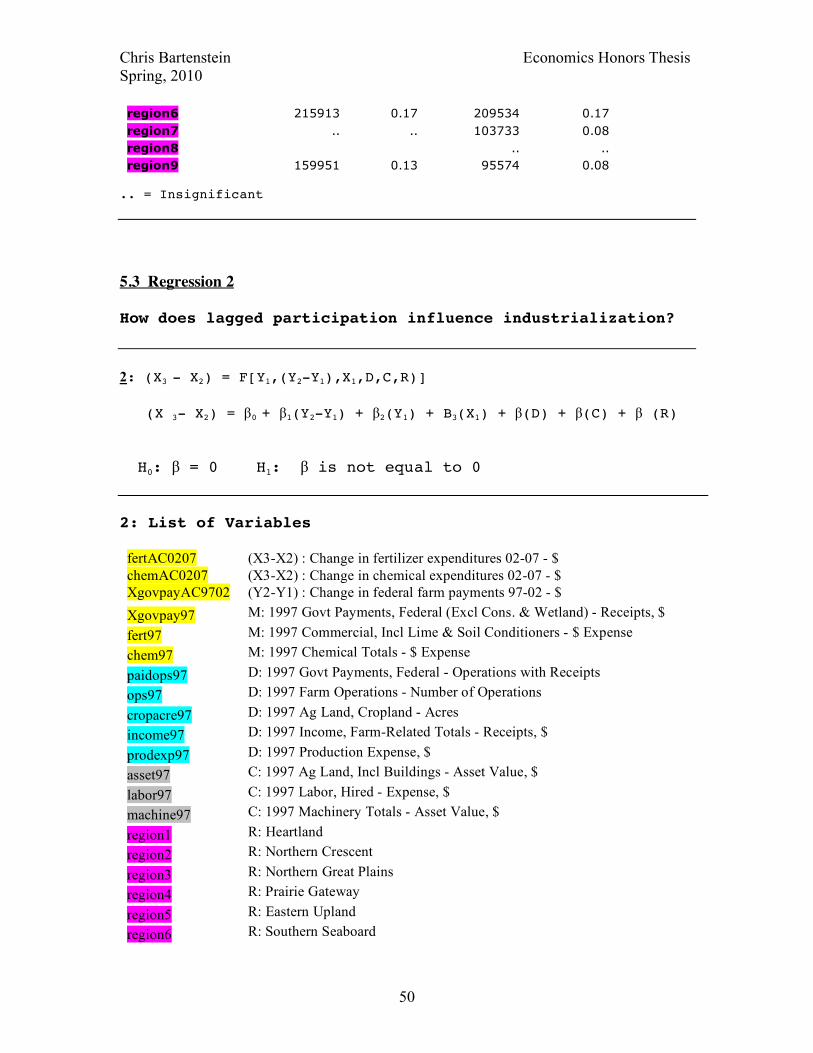
Chris Bartenstein Economics Honors Thesis Spring, 2010
50
region6 215913 0.17 209534 0.17 region7 .. .. 103733 0.08 region8 .. .. region9 159951 0.13 95574 0.08 .. = Insignificant
5.3 Regression 2
How does lagged participation influence industrialization?
2: (X3 - X2) = F[Y1,(Y2-Y1),X1,D,C,R)]
(X 3- X2) = β0 + β1(Y2-Y1) + β2(Y1) + B3(X1) + β(D) + β(C) + β (R)
H0: β = 0 H1: β is not equal to 0
2: List of Variables
fertAC0207 (X3-X2) : Change in fertilizer expenditures 02-07 - $ chemAC0207 (X3-X2) : Change in chemical expenditures 02-07 - $ XgovpayAC9702 (Y2-Y1) : Change in federal farm payments 97-02 - $ Xgovpay97 M: 1997 Govt Payments, Federal (Excl Cons. & Wetland) - Receipts, $ fert97 M: 1997 Commercial, Incl Lime & Soil Conditioners - $ Expense chem97 M: 1997 Chemical Totals - $ Expense paidops97 D: 1997 Govt Payments, Federal - Operations with Receipts ops97 D: 1997 Farm Operations - Number of Operations cropacre97 D: 1997 Ag Land, Cropland - Acres income97 D: 1997 Income, Farm-Related Totals - Receipts, $ prodexp97 D: 1997 Production Expense, $ asset97 C: 1997 Ag Land, Incl Buildings - Asset Value, $ labor97 C: 1997 Labor, Hired - Expense, $ machine97 C: 1997 Machinery Totals - Asset Value, $ region1 R: Heartland region2 R: Northern Crescent region3 R: Northern Great Plains region4 R: Prairie Gateway region5 R: Eastern Upland region6 R: Southern Seaboard
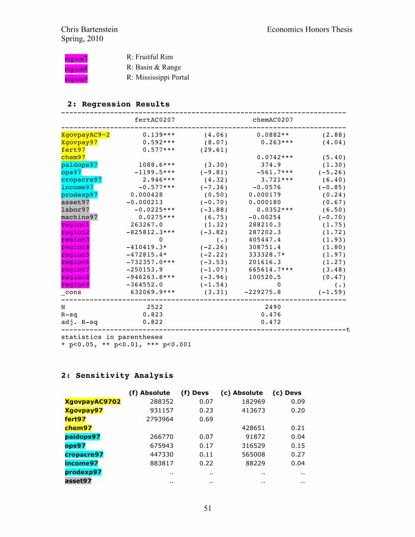
Chris Bartenstein Economics Honors Thesis Spring, 2010
51
region7 R: Fruitful Rim region8 R: Basin & Range region9 R: Mississippi Portal 2: Regression Results
---------------------------------------------------------------------- fertAC0207 chemAC0207 ---------------------------------------------------------------------- XgovpayAC9~2 0.139*** (4.06) 0.0882** (2.88) Xgovpay97 0.592*** (8.07) 0.263*** (4.04) fert97 0.577*** (29.61) chem97 0.0742*** (5.40) paidops97 1088.6*** (3.30) 374.9 (1.30) ops97 -1199.5*** (-9.81) -561.7*** (-5.26) cropacre97 2.946*** (4.32) 3.721*** (6.40) income97 -0.577*** (-7.36) -0.0576 (-0.85) prodexp97 0.000428 (0.50) 0.000179 (0.24) asset97 -0.000213 (-0.70) 0.000180 (0.67) labor97 -0.0225*** (-3.88) 0.0352*** (6.50) machine97 0.0275*** (6.75) -0.00254 (-0.70) region1 263267.0 (1.32) 288210.3 (1.75) region2 -825812.3*** (-3.82) 287202.3 (1.72) region3 0 (.) 405447.4 (1.93) region4 -410419.3* (-2.26) 308751.4 (1.80) region5 -472815.4* (-2.22) 333328.7* (1.97) region6 -732357.0*** (-3.53) 201616.3 (1.27) region7 -250153.9 (-1.07) 665614.7*** (3.48) region8 -946263.8*** (-3.96) 100520.5 (0.47) region9 -364552.0 (-1.54) 0 (.) _cons 632069.9*** (3.31) -229275.8 (-1.59) ---------------------------------------------------------------------- N 2522 2490 R-sq 0.823 0.476 adj. R-sq 0.822 0.472 ----------------------------------------------------------------------t statistics in parentheses * p<0.05, ** p<0.01, *** p<0.001 2: Sensitivity Analysis (f) Absolute (f) Devs (c) Absolute (c) Devs XgovpayAC9702 288352 0.07 182969 0.09 Xgovpay97 931157 0.23 413673 0.20 fert97 2793964 0.69 chem97 428651 0.21 paidops97 266770 0.07 91872 0.04 ops97 675943 0.17 316529 0.15 cropacre97 447330 0.11 565008 0.27 income97 883817 0.22 88229 0.04 prodexp97 .. .. .. .. asset97 .. .. .. ..
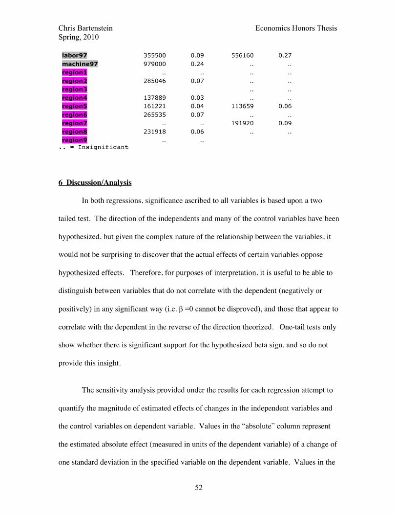
Chris Bartenstein Economics Honors Thesis Spring, 2010
52
labor97 355500 0.09 556160 0.27 machine97 979000 0.24 .. .. region1 .. .. .. .. region2 285046 0.07 .. .. region3 .. .. region4 137889 0.03 .. .. region5 161221 0.04 113659 0.06 region6 265535 0.07 .. .. region7 .. .. 191920 0.09 region8 231918 0.06 .. .. region9 .. .. .. = Insignificant
6 Discussion/Analysis
In both regressions, significance ascribed to all variables is based upon a two
tailed test. The direction of the independents and many of the control variables have been
hypothesized, but given the complex nature of the relationship between the variables, it
would not be surprising to discover that the actual effects of certain variables oppose
hypothesized effects. Therefore, for purposes of interpretation, it is useful to be able to
distinguish between variables that do not correlate with the dependent (negatively or
positively) in any significant way (i.e. β =0 cannot be disproved), and those that appear to
correlate with the dependent in the reverse of the direction theorized. One-tail tests only
show whether there is significant support for the hypothesized beta sign, and so do not
provide this insight.
The sensitivity analysis provided under the results for each regression attempt to
quantify the magnitude of estimated effects of changes in the independent variables and
the control variables on dependent variable. Values in the “absolute” column represent
the estimated absolute effect (measured in units of the dependent variable) of a change of
one standard deviation in the specified variable on the dependent variable. Values in the
Chris Bartenstein Economics Honors Thesis Spring, 2010
53
“devs” (or deviations) column represent the number of standard deviations in the
dependent variable the absolute effect noted in the “absolute” column constitute. In other
words, values in the “devs” column display the number of standard deviations in the
dependent variable a one standard deviation change in the specified variable is predicted
to produce. Regions dummies are included in the sensitivity analysis where they find
statistical significance under a two-tailed test, however the “absolute” and “dev” values
calculated for these variables don’t have any interpretable meaning; for the standard
deviation in the dummies is meaningless. To interpret the magnitude of the effect of
dummies, it makes the most sense simply to examine the coefficient assigned to each of
them.
6.1 Regression 1: Discussion
Regressions 1A and 1B attempt to estimate how changes IA over the life of the
1996 farm bill affected relative changes in participation in subsidy programs amongst
counties subsequent to the passage of the 2002 farm bill. In both 1A and 1B, proxies for
change in IA over the life of the 1996 farm bill (i.e. differences in fertilizer payments (f)
and chemical payments (c) between 1997 and 2002) 60 estimate changes in subsidy
payments starting in 2002. In 1A, we look at how these IA differences (2002-1997)
influenced changes in relative levels of participation in the year 2002 by regressing the
difference in subsidy payments between 1997 and 2002 on them in each county. In 1B,
we look at how these same IA differences influenced changes in relative levels of
60 Changes in IA that occurred between 1996 and 1997 are not technically included in these (c) and (f) datapoints, and some changes to IA occurring after passage of the 2002 farm bill leak into this statistic since the 2002 farm bill was passed during the growing season of 2002, and census data covers the 2002 growing season. Still, the statistic is assumed to capture mostly changes in IA occurring under the 1996 farm bill, and little else.
Chris Bartenstein Economics Honors Thesis Spring, 2010
54
participation between 2003 and 2007, as a consequence of the passage of the 2002 farm
bill, by regressing the difference in subsidy payments between 2002 and 2007 on them.
1A essentially captures the immediate effect (if any) of changes in IA under the 1996
farm bill on changes in relative levels of participation subsequent to the passage of the
new 2002 farm bill, while 1B captures the delayed effects (if any) of these same changes
in IA on relative levels of participation in subsidy programs amongst counties.
I interpret the dependent variable in 1A as “changes in relative levels of
participation in 2002” and not as changes in relative levels of participation between 1997
and 2002 because, between 1997 and 2001, I hypothesize only small change in relative
payment levels (minus conservation reserve payments) would have taken place. In these
years, direct payments, the core of the commodities program under the 1996 farm bill,
were tied to levels of output in years previous to 1996, which means that the farmland
eligible for participation between 1997 and 2002 did not differ from the farmland eligible
for participation in 1996. This implies that a rational farmer choosing to participate in
years between 1998 and 2002 would probably also have wanted to participate in 1997 to
reap the “free” benefits of subsidy payments, and that therefore there would not have
been much change between 1997 and 2002.
Nonetheless, a few important reservations about this interpretation deserve
disclosure. I say only “probably” because participation in direct payment programs did
entail some restrictions on growing patterns, albeit minor ones compared with the
restrictions of earlier payment programs.61 To the small group of farmers for whom these
61 See appendix D for a discussion of direct payments.
Chris Bartenstein Economics Honors Thesis Spring, 2010
55
restrictions were burdensome, participation was not “free,” and so these farmers could
rationally have justified increases or decreases in relative payment levels between 1997
and 2002 if farm conditions happened to have changed in these years. Moreover, not all
farmers are rational, and not all farmers have perfect information.62 Another important
reservation with the interpretation of 1A is that payments in each county were variable
between 1997 and 2002 on account of “emergency payments” and the like. I conclude,
however, that such payments amount mostly to noise in the long run. In the first place,
such payments were only temporary (and farmers knew this), and in the second place,
presumably they were distributed approximately proportionally to existing levels of
payments, and so did not seriously skew the relative distribution of payments.
If, for all of these reasons, changes in relative levels of payments was more
significant than supposed between 1997 and 2001, regression 1A suffers from an
endogeneity problem: reverse causality. Payment levels and IA levels are theorized to
influence one another. If changes in one occurred simultaneously with changes in the
other over the measurement period, it becomes impossible to distinguish which variable
is driving the correlation between the two, and to what extent.
A final point about regression 1A is that, even if changes in relative levels of
payments between 1997 and 2001 did not change significantly, 1A still suffers a minor
endogeneity problem: changes in payments necessarily do overlap changes in IA in the
measurement year, 2002. In this year, changes in relative levels of payments occurring
with the transition to 2002 farm bill legislation could drive changes in IA that would then
62 If these two facts were not true, regression 1B would serve no purpose.
Chris Bartenstein Economics Honors Thesis Spring, 2010
56
show up in the “change in IA, 97-02” variable, the independent variable. I conclude that
this is not a serious problem given the short period of overlap and the longer time frame
over which a change in payment levels are hypothesized to influence IA.63 A tiny amount
of the correlation between changes in IA and changes in payment levels may be due to
reverse causality, but if the effect of changes in IA between 1997 and 2002 on changes in
payments is great, the interpretation should not be significantly skewed (although the bias
is presumably toward a higher and more significant beta coefficient).
The principal purpose of regression 1 is to test the plausibility of the second
causal pathway by which federal subsidy programs are theorized to induce increases in
farmers’ levels of IA. As discussed earlier, if causal pathway 2 was operational in the
1997-2007 period, we would expect regressions 1A and 1B to find a statistically
significant beta coefficient for changes in industrialization. An insignificant or
significant negative finding for this coefficient would not support the hypothesis that
causal pathway 2 was operational during this period.
6.2 Regression 1: Analysis
R^2
Regression 1A explains much more of the linear variation in the growth of
participation in government agriculture subsidy programs value than does 1B. The most
apparent explanation for this observation is that each regression controls for 1997 values.
63 The effects of changes in payments on changes in IA in 2002 would presumably fall mostly into the category of risk-related effects stemming from a change in expected income. Structural effects are expected to be less significant since farmers would already have needed to make most of these structural changes prior to participation in order to modify relative payment levels in the first place. Risk-related changes are hypothesized to occur slowly.
Chris Bartenstein Economics Honors Thesis Spring, 2010
57
Compared with the dependent variable in 1A, the dependent variable in 1B consists of
observations further in the future, where these controls are presumably less relevant.
This explanation is incomplete because even if the 1997 controls are replaced with 2002
values in a modified 1B, r^2 in this modified 1B remains much lower than r^2 in 1A.
Another way in which to interpret the difference in the explanatory power of the two
models is to conclude that the dependent variable for 1B exhibits more inherent
randomness than the dependent variable for 1A. As with the 1996 farm bill, the 2002
farm bill stipulated payments tied to previous years’ production. As was the case in
1996, most rationally behaving farmers would have been expected to apply for as much
“free” payment as they were eligible to receive as soon as the 2002 bill passed, and to
retain these payment levels throughout the life of that bill. So, changes in relative levels
of payments occurring after 2002 may be more attributable to the irrational (and therefore
random) choices of farmers than changes in relative levels of payments occurring in
2002. Moreover, with regard to the subset of farmers for whom the costs of participation
are perceived as real given the minor restrictions they impose, rationally driven changes
in levels of participation (and therefore payments) should occur due to changes in
underlying production-based variables (e.g. factor costs) occurring after 2002, and these
changes cannot be controlled. Finally, variation in changes in payments after 2002 but
before 2007 may be proportionately more attributable to variation in temporary payment
measures that happen to overlap with the core payment programs when measurements in
2002 and 2007 are taken. Since the model does not attempt to explain these variations, if
they contribute to a greater portion of the variance of the dependent in 1B, it makes sense
that r^2 is smaller for 1B.
Chris Bartenstein Economics Honors Thesis Spring, 2010
58
The Independent Variables: Change in Fertilizer and Change in Chemicals
In terms of the estimated effect of changes in IA proxies on future changes in
participation proxies, regression models 1A and 1B run counter to the WAH. As the
theoretical narrative goes, farmers increase levels of IA as they transition toward
production methods expected to garner higher subsidy payments under the 2002 farm
bill, which in turn enables (and so causes) higher participation (and therefore payments)
after the 2002 bill is signed into law. Most farmers are expected to register transitioned
land for payments as the ink dries on the 2002 bill, but some may be more slow to act,
and may not register land until years 2003-2007. So, if the causal pathway (defined in
section 4.1) is accurate, we would anticipate that the coefficient on change in fertilizer
use and chemical use (IA proxies) would be strongly positive in regression 1A, and likely
also positive in regression model 1B. By contrast, 1A finds insignificance, and 1B shows
statistically significant negative beta coefficients for both IA proxies, although the
sensitivity analysis shows IA is not the most important factor (a 1 sd increase in these
variables yields approximately a .1 sd decrease in the dependent).
Explaining these counter-intuitive results is a challenge. One possibility is that
farmers simply do not think far enough into the future on a systematic basis to modify
levels of industrial agriculture in anticipation of future subsidy payment programs. Such
an explanation would account for the insignificant findings for 1A, but hardly accounts
for the significant negative beta value found in 1B. If farmers behave without regard to
future policy changes, changes in IA between 1997 and 2002 should have no bearing on
changes in payments between 2002 and 2007. Another possibility is that increases in IA
Chris Bartenstein Economics Honors Thesis Spring, 2010
59
between 1997 and 2002 do cause increases in payments immediately after the passage of
2002 legislation, but that our model fails to assign an appropriate beta coefficient and
significance level to the change in IA variable on account of a problem with the way in
which we have controlled the model. One possibility is that changes in IA may be
spuriously correlated with variables uncontrolled in our model that have a negative effect
on payments in 2002 (negating the otherwise positive correlation, and creating a
condition of insignificance). 2002 values were deliberately excluded as controls in our
regression so that the regression would not assign downstream effects of the independent
variable to control variables. However, their exclusion comes at the cost of increasing
the likelihood that spurious variables skew the model.
If, contravening regression 1A, increases in IA between 1997 and 2002 do cause
increases in payments subsequent to the passage of 2002, a tenable regression to the
mean explanation can be advanced for the negative coefficient in 1B. The farmers who
anticipated getting the most benefit out of future subsidy payments, and therefore
underwent the largest anticipatory increases in IA, presumably were the ones to have
overestimated the true value of producing under a subsidy payment regime. Although
these farmers may have been quick to register for payments when the 2002 bill was
newly passed, upon realizing they had overestimated the value of participation given its
continued constraints on production, they may have begun participating less (and
therefore receiving lower payments) in the years 2003-2007. On the other side of the
expectations spectrum, farmers who anticipated getting the least benefit out of future
subsidy payments, and therefore underwent the least (or even negative) anticipatory IA,
likely were the ones to have most underestimated the true value of their continued or
Chris Bartenstein Economics Honors Thesis Spring, 2010
60
additional participation in subsidy programs. Upon realizing their error in the years
following passage of the 2002 bill, these farmers may have increased participation in
subsidy programs to whatever extent possible (which probably wasn’t very much, given
the fact that they had undergone the smallest increases and biggest decreases in IA, and
industrial production is considered a prerequisite of higher levels of subsidy payments).
Irrespective of the many possible explanations for the regression findings that one
could make, it must be conceded that no evidence for causal pathway 2 is found for the
1997-2002 period. Nevertheless, regression 1 is in not entirely unsupportive of the
WAH. Although changes in IA preceding the 2002 farm bill do not appear to be
correlated with changes in participation after its passage, all regressions except 1B(f),
find baseline/1997 proxies for IA to be positively correlated with changes in
participation. In other words, the regressions show that counties with higher preexisting
levels of industrial agriculture tend to undergo greater increases in participation. This
could mean one of two things. It could mean that accumulated increases in IA do cause
increased participation over the long-term. Under this interpretation, regression model 1
simply fails to capture the effect of changes on participation either because the
investigated period was a historical anomaly, or, more likely, because changes in IA take
more than five years to significantly influence changes in participation. A second
possibility is that 1997 levels of AI do not actually influence future changes in AI and are
only spuriously correlated with changes in payments between 2002 and 2007. Unlike
changes in payments, 1997 levels of payments presumably correlate with many historical
factors that are uncontrolled in regression 1, so spurious correlation is not unlikely.
Further investigation into the effects of levels of payments on future changes in AI may
Chris Bartenstein Economics Honors Thesis Spring, 2010
61
be warranted, but not without a note of caution: historical farm data for years prior to the
1990’s needed for such an investigation are not as comprehensive as modern farm data
and are rarely available in electronic format.
Control Variables
Several of the coefficients for the control variables in regression 1 fall in line with
what one would expect, while others do not.
In both 1A and 1B, counties with more crop acres in ‘97 corresponded with
bigger increases in payments. We would expect this to be the case because a greater
number of acres equates to more farmland eligible to receive payments. Since payments
increased overall in both 1997 and 2002, the average acre received increasingly high
payments over both periods, and so more acres should on average correlate with higher
absolute subsidy payments. Moreover, since number of farms is controlled, higher total
acreage implies larger farms. Larger farm operations may have greater incentive to
increase subsidy program participation since, county payments being fixed, they have
more land to enroll than smaller operations. Larger farms also tend to practice more
industrial styles of production, but 1997 fertilizer and chemical expense variables more
directly control for preexisting levels of industrial agriculture than does number of crop
acres, so the coefficient on crop acres should not reflect the influence of preexisting
levels of county industrialization.
Chris Bartenstein Economics Honors Thesis Spring, 2010
62
Regression findings for the variable controlling for levels of payments in 1997 are
not easy to interpret, but deserve special attention since 1997 payment level ranks as one
the most decisive determinants of changes in payments based on the sensitivity analysis
in all regressions but 1B(c), where findings are insignificant. Government payments in
1997 are predicted to have a strongly negative impact on changes in payments between
1997 and 2002 and a strongly positive effect on changes in payments between 2002 and
2007. Regression to the mean may explain the strong negative correlation in 1A.
Counties in which farmers already received high payments (controlled for by total
number of crop acres in that county) experience stable or declining government payments
because all or nearly all of their acres are already enrolled in subsidy programs; these
farmers have already reached a ceiling on possible subsidy payments. Interpreting the
highly significant (significant at the .1% level) positive coefficient on 1997 payments in
regression 1B(f) is more difficult. Further complicating matters is the finding in
regression 1B(c) that payment level is not significant at the 5% level. Regressions 1B(c)
and 1B(f) differ only in terms of the proxy used for measuring AI. Coefficients for the
control variables should not differ substantially between 1B(f) and 1B(c) if both proxies
do in fact measure the same underlying phenomenon. I can think of no good explanation
for the positive coefficient or for the difference in statistical significance for the payment
variable.
A story can also be threaded to explain the regression findings for the variables
controlling number of total farm operations in a county and number of paid farm
operations in a county. These two variables must be interpreted together because it
appears that each conveys meaning in terms of the other, which is to say that the actual
Chris Bartenstein Economics Honors Thesis Spring, 2010
63
total number of operations and the actual number of paid operations are not so important
as is the ratio of paid operations to total operations. The results from 1A and 1B imply
that as this ratio increases, increases in subsidy payments between 2002 and 2007 are
greater, and decreases in subsidy payments between 2002 and 2007 are smaller. The
ratio of paid operations in a county conveys information that is similar to the total amount
of payments in a county; it provides a clue as to whether a given county has historically
participated much or little in subsidy programs. However since total number of
payments per acre in ’97 is held fixed in the regression by two other variables (total
number of acres and total payments in 97), the interpretation of this variable is slightly
different. Relative to farmers in counties where a low percentage of farmers receive any
payments at all, holding payments per acre fixed, farmers in counties where a high
portion of operations receive at least some payments are likely more knowledgeable
about subsidy programs opportunities, and are at least open to the possibility of
increasing participation (since they must have done so in the past to be participating at
all).
The regressions show that for both periods regions with higher income levels
(controlled for by production expenses) tended to exhibit greater increases in received
subsidy payments. In other words, subsidy payments are increasing at a faster rate in
counties where farmers enjoy a higher income. One possible explanation for this is that
higher current income reflects greater attention to income generating opportunities.
High-income farm operators therefore are likely more aware of the potential for
increasing future income by enrolling in subsidy programs. This would imply that higher
income farmers tend to increase participation in subsidy programs at a faster rate if
Chris Bartenstein Economics Honors Thesis Spring, 2010
64
rational expectation would lead the average farmer to conclude that greater participation
would generate increased income. Also, higher income farmers tend to be wealthier
farmers, and wealthier farmers may be better able to afford conversion to more industrial
styles of farming, which the WAH theorizes is a prerequisite of garnering high subsidy
payments.
Relative factor expense levels correspond to production style, and perhaps to the
types of crops that farmers are growing. All regressions find machinery asset value to be
positively correlated with changes in payments, and all regressions besides1B(c) find
labor expense to be negatively correlated with changes in payments. This implies that
capital-intensive farm operations were predicted to increase participation by a greater
amount (or decrease participation by a lesser amount) than were labor-intensive farm
operations. One would expect that this would be the case since capital intensive farm
operations are theorized to be more amenable to the production of commodity crops in
accord with the stipulations of farm bills than more labor intensive farms.
The two regions most highly associated with increases in payments under both
regressions are regions 9 and 6 – “Mississippi portal” and “southern seaboard”,
respectively.
6.3 Regression 2: Discussion
Regression 2 attempts to estimate how changes in government payments over the
life of the 1996 farm bill and during the first growing season of the 2002 farm bill
affected relative changes in IA amongst counties subsequent to the passage of the 2002
Chris Bartenstein Economics Honors Thesis Spring, 2010
65
farm bill. In regression 2, the difference between 2002 census observations of proxies for
industrial agriculture and 2007 census observations are regressed on changes in payment
levels between 1997 and 2002 (the difference between 2002 census observations and
2007 census observations). Two separate regressions are run. One, (c), uses changes in
“chemical” expenses as the ”change in IA” proxy; the other, (f), uses fertilizer expenses
as the “change in IA” proxy. All other variables (the independent variable and all control
variables) do not differ between these regressions. These homologous regressions are
both referred to simply as “regression 2” since they test for exactly the same thing. If
fertilizer expense and “chemical expense” both accurately measure the same underlying
phenomenon, AI, then although the values of coefficients on the control variables may
differ between the two regressions, we would not expect the regressions to find
statistically significant beta coefficients of opposite directions for the control variables
(i.e. we would not expect that one regression finds statistically significant positive
correlation on a given control variable, while the other regression finds statistically
significant negative correlation on that same variable, or vice versa).
The principal purpose of regression 2 is to test the plausibility of the first causal
pathway by which government subsidy programs are theorized to increase farmers’ levels
of IA. As discussed earlier, if causal pathway 2 was operational in the 1997-2007 period,
we would expect regressions 1A and 1B to find a statistically significant beta coefficient
for changes in industrialization. An insignificant or significant negative finding for this
coefficient would not support the hypothesis that causal pathway 2 was operational
during this period.
Chris Bartenstein Economics Honors Thesis Spring, 2010
66
6.4 Regression 2 Analysis
R^2 (Comparing Regression 2 Variants)
According to r^2 values on the two variants of regression 2 (one using changes in
fertilizer expenses (f) as the dependent variable, and the other using changes in
“chemical” expenses (c) as the dependent variable), variation in changes in federal
subsidy payments and control variable values collectively explain substantially more of
the linear variation in changes in fertilizer expenses than changes in “chemical” expenses.
Although chemical expense and fertilizer expense both serve as proxies for IA, neither
perfectly characterizes what alternative agriculturalists understand to mean AI.64
Consequently, these two proxies are not perfectly correlated (although they are strongly
correlated), and the causal pathways resulting in changes to one resemble, but do not
match, the causal pathways resulting in changes to the other. Thus, a difference in the
R^2 value between the two variants is to be expected, but the magnitude of the difference
is surprisingly large (.82 vs .48).
One or both of two possible scenarios must explain this difference. In the first
scenario, significant variables influencing changes in chemical expenses have been left
out of the regression. In the second scenario, a higher percentage of the change in
chemical payments is random. Greater randomness in the variance of the “chemical”
64 The statement implicitly assumes such a consensus even exists. Realistically there is no perfect consensus as to the meaning of AI. Agricultural industrialization describes a group of abstract and related concepts, and so quantifying its values essentially amounts to an exercise in estimation even where its characteristic manifestations can be observed.
Chris Bartenstein Economics Honors Thesis Spring, 2010
67
expense dependent variable may account for some of this difference,65 but it seems
unlikely the randomness explanation accounts for all of this difference. Farmers
presumably make decisions about how much to spend on “chemicals” in much the same
way as they choose how much to spend on fertilizer: they select the chemical/fertilizer
expense where the expected marginal return on an additional unit of chemical/fertilizer
expense equals its cost. So, claims that a large portion of the variance in chemical
payments is randomly determined appear doubtful. Which critical variables have been
omitted in the chemical payments variant of regression 2 is a matter of speculation.
Presumably, these omitted variables do not correlate highly with any of the preexisting
independent/control variables,66 so entirely exogenous variables, such as weather
patterns, rank as the most likely candidates. Although, if weather were the missing
variable, we would expect the regions’ dummies to find more, not less, significance in the
chemicals variant of the regression model since these dummies are the only variables
even remotely related to differences in weather patterns. Notably, the sensitivity
analysis for regression 2 finds base/1997 levels of fertilizer expense to be a much more
critical determinant of future changes in levels of fertilizer expense than base/1997 levels
of chemical expense is to future changes in levels of chemical expense.
65 Of course, some might argue that the occurrences of real world events are never truly random, in whole or in part. This point is difficult to contest, but it seems perfectly reasonable to consider random that portion of variation attributable to a near infinite number of correlated and related variables in a statistically insignificant way. For example, the weather may not truly be random, but it might as well be – for it can not be predicted with accuracy further out than a couple of days.
66 Otherwise, we would already have a high r^2 value on the chemicals variant of regression 2 due to false attribution of causal variance to the correlated variables
Chris Bartenstein Economics Honors Thesis Spring, 2010
68
The Independent Variable: Change in Subsidy Payment Level
Regression model two finds considerably more support for the first causal
pathway by which government subsidy programs have been theorized to increase AI than
does regression model one for the second causal pathway. Both variations on regression
model two find that increases in government payments between 1997 and 2002 resulted
in increases in the applicable proxy or AI between 2002 and 2007. The findings match
theory in this regard. Increases in relative levels of participation between 1996 and 2002
(including changes in participation that took place over the first growing season under the
2002 farm bill) were correlated (presumably causally) with increases in the rate at which
farmers industrialized their operation between the end of 2002 and 2007. That the r^2
value exceeds .8 in the fertilizer variant of regression 2 suggests that this regression
manages to include most of the important variables responsible for determining levels of
AI, and that there is a low likelihood that payments are spuriously correlated (i.e.
correlated in an acausal manner). Spurious correlation threatens to be more of an issue in
the chemical variant of regression 2. But the similarity in the magnitude of the effect
accorded the change in payments variable in both variants (.07 “devs” vs. 09 “devs”)
suggests that the effect found in the regression may indeed reflect the true effect of
changes in lagged subsidy payments on changes in production-based measurements of
AI. This finding implies that the second causal hypothesis is accurate, and so supports
the WAH.
The fact that regression 2 also assigns a statistically significant positive
coefficient to baseline/1997 levels of chemical payments and fertilizer payments (in the
respective regression variants) also appears supportive of the WAH. This finding implies
Chris Bartenstein Economics Honors Thesis Spring, 2010
69
that the farmers with a history of participating in subsidy programs in a big way tend to
undergo AI at a faster rate than farmers with a history of participating little in subsidy
programs. The finding implies that the effects of increases in IA may take many years to
render their full effect on levels of IA. For, higher 1997 payment levels of IA can
ultimately be attributed to historical increases in participations less historical decreases in
participation. Although, as was the case with the base/1997 IA proxy variables in
regression 1, the danger with leaping to such a conclusion is that 1997 payment levels are
not well controlled. Theoretically, they could merely be exhibiting spurious correlation
with changes in IA.
Control Variables
The statistically significant positive coefficients found on proxies for base-level
IA contradict the theorized effect of preexisting levels of AI on future AI. In his
research, MacCannell found that higher levels of IA were associated with slower rates of
AI, which he concluded made perfect sense. According to MacCannell, the most
industrialized farms reach a ceiling in IA, at which point they are no longer are able to
further industrialize. So, he theorized that the least industrial farmers tend to under AI at
the fastest rates. Perhaps this was true in the 1980’s, the period analyzed in the
MacCannell study, but apparently this no longer is true. Both variants of regression 2
find that higher levels of IA in 1996 resulted in larger increases in IA between 2002 and
2007. Although this finding opposes the theory, it does not seem unjustifiable.
Advancing technology and changes in standard farming practice over time rule out the
existence of a permanent, fixed ceiling in levels of IA. The most industrialized farm
operations are presumably those managed by the group of farmers most knowledgeable
Chris Bartenstein Economics Honors Thesis Spring, 2010
70
about the potential advantages of AI,67 so it makes sense that in counties already
exhibiting high IA would continue to industrialize at a faster rate than counties with
lower baseline IA. Moreover, even if a ceiling is reached on highly industrialized farm
acreage, farm managers running industrial operations can purchase less industrialized
farmland and begin industrializing production on that acreage. Finally, in recent times
there been a movement among a small, but growing cohort of farmers to reduce IA as
part of a conversion to more “alternative” modes of production. It would seem
reasonable to expect that the farm operations registering decreases in IA tend not to have
been most industrialized operations to begin with.
As with regressions 1A and 1B, the ratio of paid operations to total operations
holds more meaning than do either of these control variables independent of one another.
According to regression 2, as this ratio increases, increases in fertilizer expenses and
chemical expenses in counties between 2002 and 2007 are predicted to be larger. This
finding makes sense for much the same reason as the analogous finding in regressions 1A
and 1B made sense. If subsidy payments are indeed related to IA in the ways that have
been proposed throughout the thesis, counties where a relatively high percentage of
farmers receive relatively high subsidy payments are also expected to be counties where a
relatively high percentage of farmers farm exhibit relatively high levels of IA. Farmers
are more likely to be influenced by the practices of nearby farmers than by the practices
of distant farmers. A farmer growing moderately industrially may be swayed to grow
extremely industrially in counties where most other farmers farm grow their produce
67 These farmers are, perhaps, also the least knowledgeable about the potential advantages of alternative farming methods.
Chris Bartenstein Economics Honors Thesis Spring, 2010
71
extremely industrially, or to farm less industrially in counties where alternative styles of
production are the norm. So, in counties where the ratio of paid operations to total
operations is high, a higher rate of AI would be expected, and is predicted.
Regression two finds 1997 Income levels to be negatively correlated with
increases in fertilizer expenses between 2002 and 2007 in a statistically significant
fashion. This implies that farmers with higher incomes are expected to increase fertilizer
expenditures by lesser amounts or to increase fertilizer expenditures by a greater amount
between 2002 and 2007 relative to a farmer with lower income. This is an interesting
finding. Higher earning farmers have more money to spend on variable capital inputs
(e.g. fertilizer, chemicals), and so one would expect that farmers earning a higher income
would tend to undergo larger increases in fertilizer expenditure relative to other farmers.
Such a finding is also odd in light of the fact that regression 1 found higher income to be
associated with larger increases in subsidy payments. Reverse causality is one possible
explanation for the finding on income level in the fertilizer variant of regression 2.
Smaller increases in expenditures on synthetic fertilizer (or larger decreases in these
expenditures) may signify cost efficient production. This finding also provides grounds
for investigation into the possibility that less industrial modes of production (or, at least,
those which use less synthetic fertilizer) are more profitable. The beta coefficient on
1997 income level is not significant when changes in chemical expenses are used as the
regressand.
According to regression 2, counties with more crop acres in 1997 underwent
larger increases in both fertilizer and chemical expenses than did counties with few crop
Chris Bartenstein Economics Honors Thesis Spring, 2010
72
acres. Since chemical and fertilizer expenditure increased overall between 2002 and
2007, the average acre exhibited higher fertilizer/chemical expenditures over the period.
So more acres should, on average, correlate with larger increases in these expenditures in
counties. Moreover, since number of farms is controlled, higher total acreage implies
larger farms. Larger farms tend to practice more industrial styles of production, but
baseline/1997 fertilizer and chemical expense variables more directly control for
preexisting levels of industrial agriculture than does number of crop acres, so the
coefficient on crop acres should not reflect the influence of preexisting levels of county
industrialization. It is not clear whether or not farm size had any independent effect on
county changes in AI between 2002 and 2007.
As pointed out in 6.2, relative factor expense levels correspond to production
style, and perhaps to the types of crops that farmers were growing at the time.
Regression 2’s results suggest no obvious, coherent interpretation of what the effects of
production style on changes in fertilizer expenses or chemical expenses may be. There is
likewise no obvious story to be drawn from the coefficients assigned to the region
dummy variables in the two regressions.
7 Conclusion
The results from regressions 1 and 2 collectively provide weak and tentative
support for the claim by alternative agriculturalists that subsidy programs are responsible
for high, and ever increasing levels of IA at the national level. Support is only tentative
because the regressions did not directly address the principal criticism lodged by the
Chris Bartenstein Economics Honors Thesis Spring, 2010
73
alternative movement against federal farm subsidies.68 Rather, regressions 1 and 2 test a
related, but distinct set of propositions (or, proposed causal pathways): 1) that
expectations of future participation in subsidy programs causes increases IA and 2) that
participation in current subsidy programs cause increases in IA. Collectively, these
postulates are known as the weak alternative hypothesis, or the WAH.
Support for the SAH is weak because regressions 1 and 2 provide only weak
support for the WAH. In regression 1, changes in participation are regressed on lagged
changes in IA to test for the validity of proposition 2, and in regression 2, changes in IA
are regressed on lagged changes in participation to test for the validity of proposition 1.
Regression 2 finds strong support for causal pathway1, but regression 1 does not find
statistically significant evidence for causal pathway 2.
As regards the overall relationship between individual farmers, their participation
in subsidy programs, and their level of IA the regressions support the following
conclusion: increased participation does cause increases in IA, but increases in IA do not
precipitate increase in participation because farmers are not sufficiently far-sighted or do
not have enough information to behave predictably in anticipation of increases in IA.
The findings from regressions 1 and 2 may also serve to undermine the theory laid out
section 3.1, which stated AI effectively constitutes a prerequisite for participation in
subsidy programs. If farmers are able to increase participation without increasing levels
of industrial agriculture beforehand, this would suggest either that AI is not a prerequisite
of participation in subsidy programs, or that farmers systematically behave irrationally by 68 This primary criticism is defined formally in 2.1 and is referred to as the “strong alternative hypothesis” or simply, the “alternative hypothesis.”
Chris Bartenstein Economics Honors Thesis Spring, 2010
74
failing to accept subsidy payments on farmland where they already meet all of the
requirements of enrollment (or, in other words, unless farmers systematically pass up on
free income).
Another possibility is that regression 1’s failure to find a significant,
positive coefficient on changes in IA can be attributed to flaws in the regression’s design.
Several of the problematic features of regressions 1 and 2, which are discussed
throughout section 4, could result in type one or type two errors. These problematic
features include susceptibility to several forms of endogeneity (for example, endogeneity
attributable by autocorrelation in base-level variables and independent variables, and
endogeneity attributable to reverse causality), sample selection bias69, spurious variables,
and inappropriate inclusion of control variables that draw away correlation causally
attributable to the independent variable.
Another potential issue with our regressions is not so much a problem with its
design as a complication endemic to all statistical research into how one variable
influences another variable over time: there is no foolproof way of knowing the correct
time frame over which the one variable influences the other.70 As discussed in section 4,
it may be the case that the independent variables influence the dependent variables in the
regressions in different ways at different points in time. The fact that 1997 levels of IA,
if not changes in IA between 1997 and 2002, were found to be strongly positively
correlated with future increases in payments in regression 1, and that 1997 levels of
69 Data on counties for which summary data uniquely identifies an individual farm operation are disclosed. 70 Theory helps, but there is no way to verify whether theory is accurate.
Chris Bartenstein Economics Honors Thesis Spring, 2010
75
payments were found to be strongly positively correlated with future increase in IA in
regression 2 suggest that these independents may influence changes in IA in different
ways over a time frame longer than the one specified for all of the regressions (one
census period immediately following--or simultaneous to--the census period over which
the independent variable is measured).
Refinements and variations on my regressions could potentially provide
additional insight into the overall effect of federal subsidy programs on AI. Incorporating
data from additional censuses would enable a researcher to experiment with different lags
to see how the effects of variables on one another change over time. Investigating the
effects of individual payment programs (rather than the effects of cumulated payments,
flowing from every federal payment programs aside from conservation reserve programs)
would also be an option worth exploring, assuming county level data on different levels
of receipts flowing from different types of government payment programs can be
acquired. Finally, original research by agricultural economists suggests that the
incorporation of three additional control variables might add value to future studies of a
similar nature as they are thought especially significant determinants of AI. These
variables are: crop insurance discount rates,71 a variable signifying the age makeup of
71 John K. Horowitz and Erik Lichtenberg, “Insurance, Moral Hazard, and Chemical Use in Agriculture,” American Journal of Agricultural Economics, Vol. 75, No. 4 (Nov., 1993), pp. 926-935.
Chris Bartenstein Economics Honors Thesis Spring, 2010
76
farmers in different county.72 Variables signifying the crop profile of different counties
might also provide useful results.
Realistically, however, this author is of the opinion that the interrelationships
between variables are too complex, and the published data are too sparse (census
observations are published on average once every five years) for researches to make
much additional headway toward evaluating the alternative hypotheses (strong and weak)
using census data – even if non-electronic, historic data are successfully gathered.
Researchers would be better served looking for natural experiments for which data exists
than continuing to manipulate census data.73
To summarize, this thesis provides preliminary evidence suggesting there may be
something to the alternative critique of federal subsidy programs, but more research is
needed. Further investigation into the relationship between federal farm subsidy
programs should focus firstly on refining theory, and secondly on finding natural
experiments with which to test theory.
72 Dimitri Damianos and Dimitri Skuras, “Farm Business and the Development of Alternative Farm Enterprises: An Empirical Analysis in Greece,” Journal of rural Studies, Vol. 12, Issue 3, July 1996, 273-283.
S. Comer, E. Ekanem, M. Safdar, S. Singh, F. Tegegne, “Sustainable and Conventional Farmers: A Comparison of Socio-Economic Characteristics, Attitude, and Beliefs,” Journal of Sustainable Agriculture, Vol. 15, No. 1, 1999, 29-45.
“The results suggest that sustainable farmers were younger and have more off-farm income compared to conventional farmers.” Ibid. Abstract: http://bubl.ac.uk/ARCHIVE/journals/jsusagr/v15n0199.htm.
73 Professors Siegfried and Crucini, you’ve been telling me this all along. I guess it just took me three semesters to arrive at the same opinion.
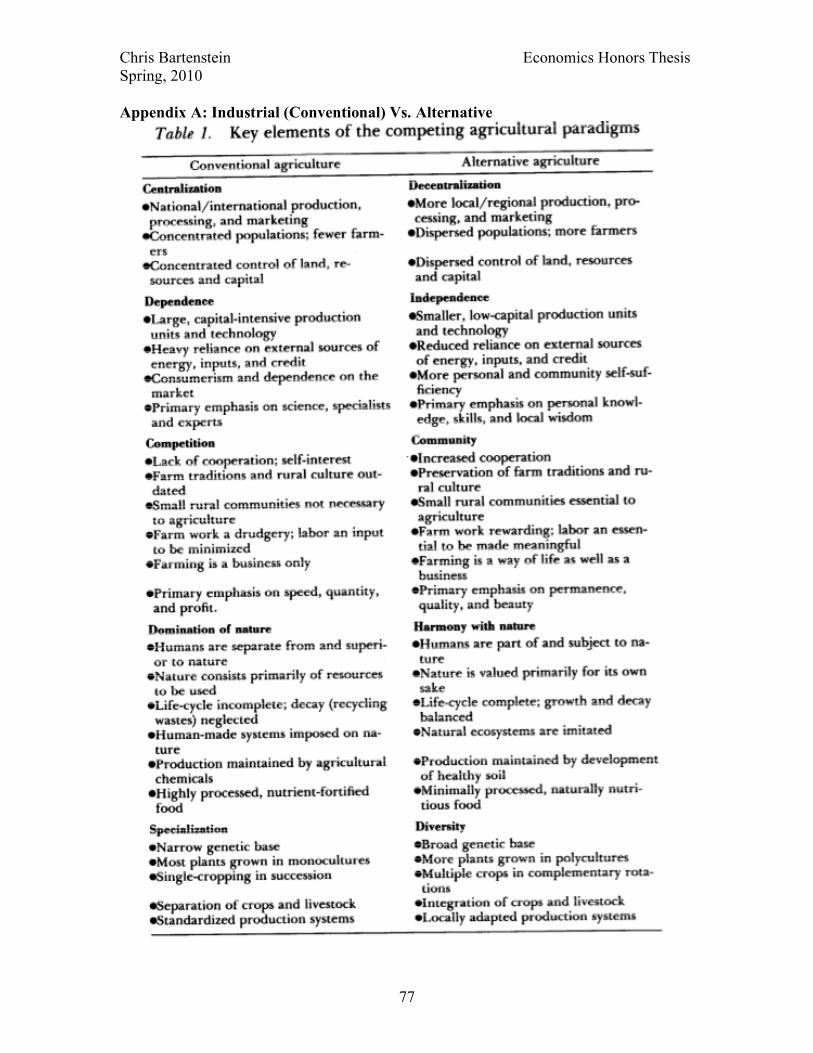
Chris Bartenstein Economics Honors Thesis Spring, 2010
77
Appendix A: Industrial (Conventional) Vs. Alternative
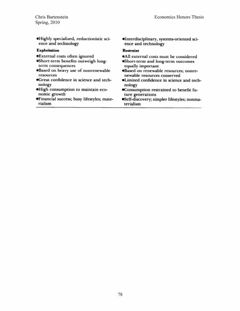
Chris Bartenstein Economics Honors Thesis Spring, 2010
78
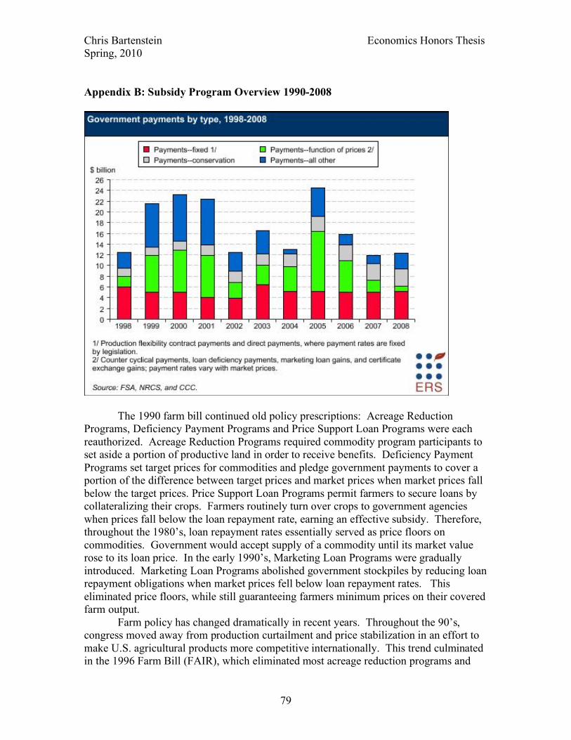
Chris Bartenstein Economics Honors Thesis Spring, 2010
79
Appendix B: Subsidy Program Overview 1990-2008
The 1990 farm bill continued old policy prescriptions: Acreage Reduction Programs, Deficiency Payment Programs and Price Support Loan Programs were each reauthorized. Acreage Reduction Programs required commodity program participants to set aside a portion of productive land in order to receive benefits. Deficiency Payment Programs set target prices for commodities and pledge government payments to cover a portion of the difference between target prices and market prices when market prices fall below the target prices. Price Support Loan Programs permit farmers to secure loans by collateralizing their crops. Farmers routinely turn over crops to government agencies when prices fall below the loan repayment rate, earning an effective subsidy. Therefore, throughout the 1980’s, loan repayment rates essentially served as price floors on commodities. Government would accept supply of a commodity until its market value rose to its loan price. In the early 1990’s, Marketing Loan Programs were gradually introduced. Marketing Loan Programs abolished government stockpiles by reducing loan repayment obligations when market prices fell below loan repayment rates. This eliminated price floors, while still guaranteeing farmers minimum prices on their covered farm output.
Farm policy has changed dramatically in recent years. Throughout the 90’s, congress moved away from production curtailment and price stabilization in an effort to make U.S. agricultural products more competitive internationally. This trend culminated in the 1996 Farm Bill (FAIR), which eliminated most acreage reduction programs and
Chris Bartenstein Economics Honors Thesis Spring, 2010
80
decoupled most payments from levels of production. The goal of the 1996 farm bill was to open U.S. agriculture to market forces by weaning farmers off of distorting price and income supports. In anticipation of increased access to export markets (so called “automatic stabilizers”), Congress planned to phase-out most remaining payment programs after 1996. However, agricultural prices plummeted between 1996 and 2000, and Congress recoiled, approving a number of emergency agricultural income-support programs. When it came time to draft the 2002 Farm Bill, policymakers reintroduced a price sensitive payment scheme called the counter-cyclical payment program. Although the program constituted a partial retreat from the free market principles of FAIR, the counter cyclical payments program is thought to be less distorting than older price sensitive payment programs since payments are tied to historic levels of production.
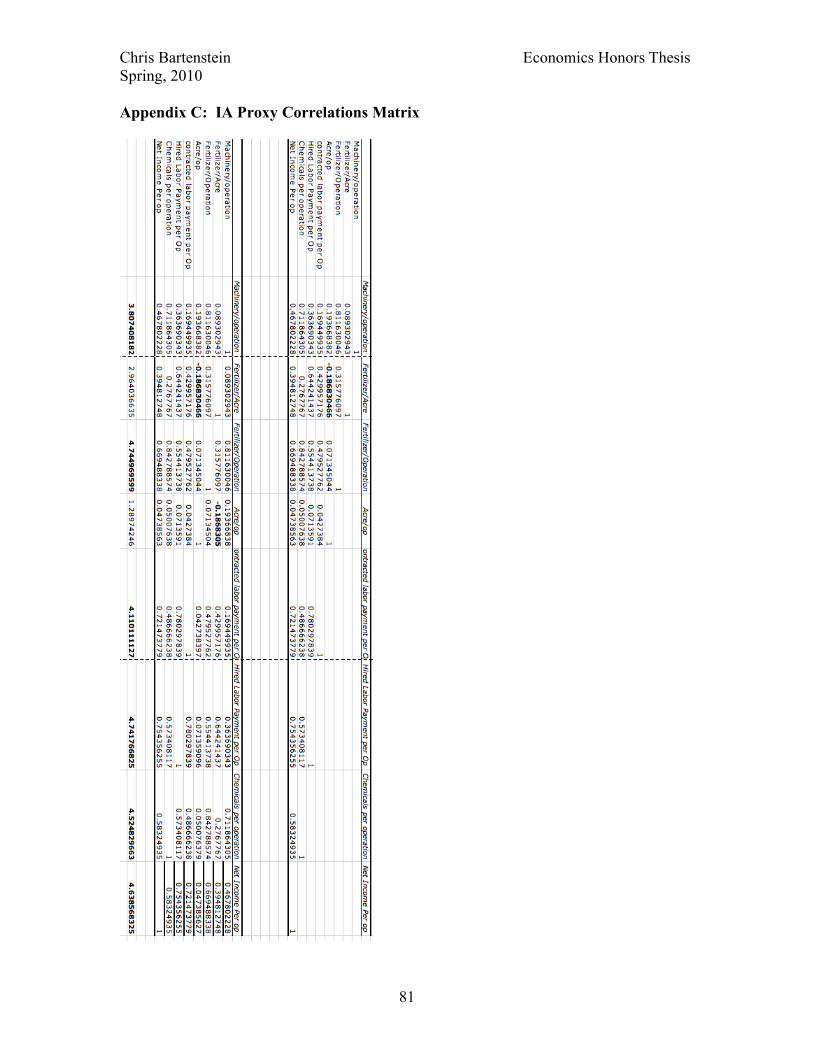
Chris Bartenstein Economics Honors Thesis Spring, 2010
81
Appendix C: IA Proxy Correlations Matrix
Chris Bartenstein Economics Honors Thesis Spring, 2010
82
Appendix D: Modeling the Effects of Subsidy Programs
Agricultural industrialization can be decomposed into four distinct components: 1) The net effect of changes in subsidy program rules and regulations on industrialization to the portion of subsidy participation that does not change over the defined period (E1) 2) the net effect of changes in participation in federal subsidy programs on industrialization over the defined period74 ( E2) 3) the net effect of anticipation of future program opportunities on industrialization with respect to both current and potential future participants (E3) 4) the “autonomous” rate of industrialization (which is the slope of Y2) multiplied by the length of the defined period (E4). E3 can be further subdivided into E3A, the net effect of anticipation eventually resulting in changes in participation on A.I., and E3B, the net effect of anticipation that never leads to changes in participation on A.I.. The slope of Y1 equals E1 + E2 + E3 + E4.
E1, E2, and E3A account for all of the change in Y1 owing to subsidy programs, but only E2 and E3B are useful for gaining insight into the absolute effect of government subsidy programs (which is tantamount to insight into the validity of the alternative model). E1 is not helpful because it measures the relative effect of current legislative conditions vs. past legislative conditions rather than the absolute effect of legislation on industrialization in a given period. This is a fancy way of saying that E1 takes measurements off of an unknown baseline. E1 may be negative subsequent to major reductions in subsidy support offered farmers, but the absolute effect of remaining subsidy programs could still be positive (i.e. observed IA, green, may still exceed baseline IA, orange, in figure 3). So, E1 provides no insight into the validity of the “alternative hypothesis.” E3B likewise provides little useful insight into the absolute direction of the long-run effect of farm subsidy programs on IA. The fact that these anticipatory changes do not actually result in changes in participation implies either that farm programs didn’t match the initial expectations of these farmers or that these farmers have since changed their minds about optimal production strategies. Hence anticipation-based fluctuations in industrialization not resulting in changes in participation are theorized to be the transitory byproduct of erroneous predictions about the future. As soon as the error is realized, attendant changes is IA are predicted to undergo reversal, canceling out the long-term effect on IA of E3B. The possible scenarios that could play out as a result of rational-expectations-driven, anticipatory IA are diagramed in a flow chart in Appendix E.
The delineation of three separate causal pathways is useful because E2 and E3A, and the interaction between the two make up the entire effect on changes in A.I. of government subsidy programs. Summing the amount by which farmers consciously modify the level of I.A. practiced on their farms in anticipation of future subsidy program opportunities75 and the amount by which they actually industrialize in the years immediately following observed changes (both on account of changed expectations about the present value of future participation in subsidy programs under future farm bills and
75 This value could be negative where a farmer no longer believes the present value of future payments exceeds the current cost of sustaining practices believed necessary for sustained future program payments.

Chris Bartenstein Economics Honors Thesis Spring, 2010
83
the risk-mediated effect of subsidies on AI) yields the net estimated effect of subsidy programs on AI. 76 Causal Pathway 1 (depicted by orange arrows in the figure on the following page) accounts for the E3A effects of government subsidy programs on changes in AI. Causal pathway (depicted by red arrows) accounts for the E2 effects of government subsidy programs on changes in AI.
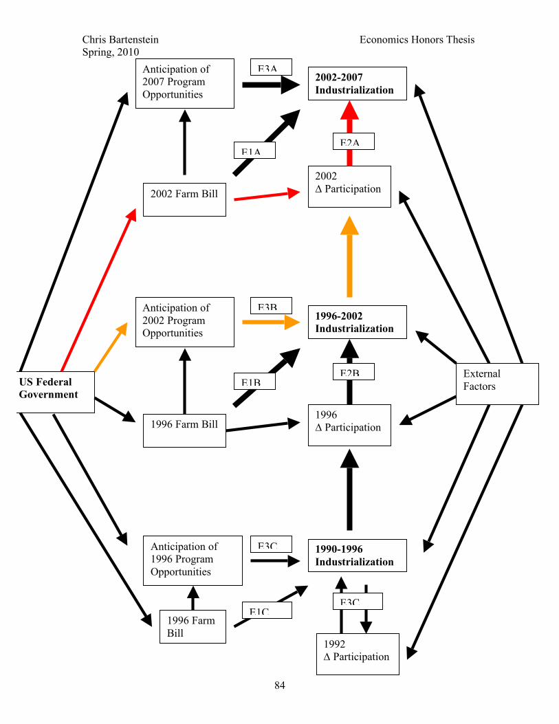
Chris Bartenstein Economics Honors Thesis Spring, 2010
84
2002 ∆ Participation
2002-2007 Industrialization
Anticipation of 2002 Program Opportunities
Anticipation of 2007 Program Opportunities
1996 Farm Bill
1996-2002 Industrialization
1996 ∆ Participation
External Factors
Anticipation of 1996 Program Opportunities
1990-1996 Industrialization
1992 ∆ Participation
US Federal Government
E3C
E1B E2B
E1C E3C
E1A E2A
E3B
2002 Farm Bill
1996 Farm Bill
E3A
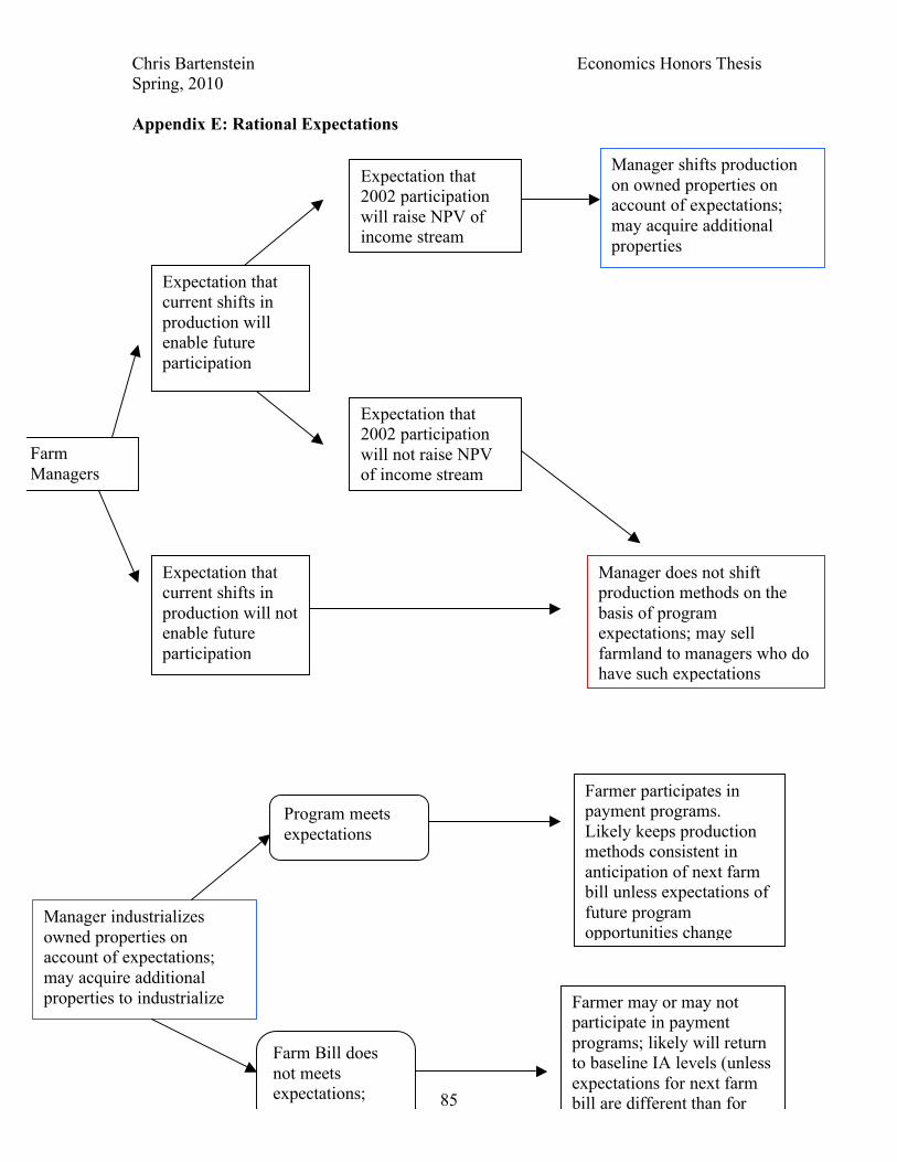
Chris Bartenstein Economics Honors Thesis Spring, 2010
85
Appendix E: Rational Expectations
Farm Managers
Expectation that 2002 participation will raise NPV of income stream
Expectation that 2002 participation will not raise NPV of income stream
Expectation that current shifts in production will enable future participation
Manager shifts production on owned properties on account of expectations; may acquire additional properties
Expectation that current shifts in production will not enable future participation
Manager does not shift production methods on the basis of program expectations; may sell farmland to managers who do have such expectations
Manager industrializes owned properties on account of expectations; may acquire additional properties to industrialize
Farm Bill does not meets expectations;
Program meets expectations
Farmer participates in payment programs. Likely keeps production methods consistent in anticipation of next farm bill unless expectations of future program opportunities change
Farmer may or may not participate in payment programs; likely will return to baseline IA levels (unless expectations for next farm bill are different than for current bill)
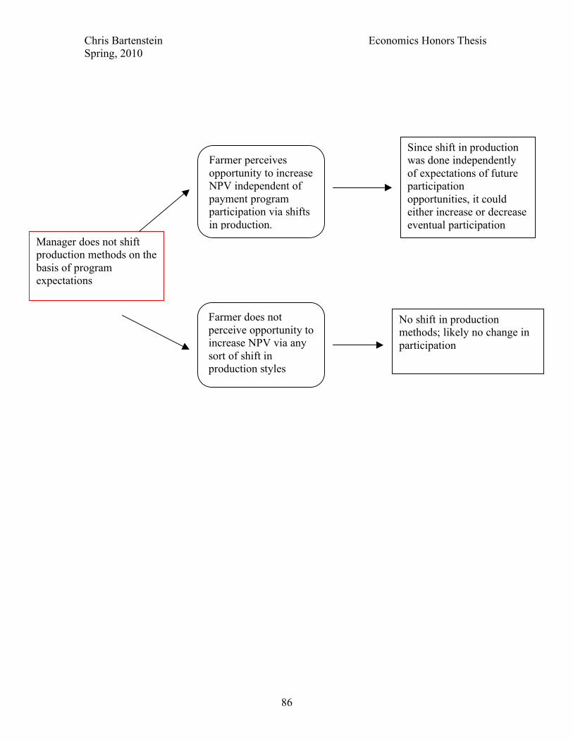
Chris Bartenstein Economics Honors Thesis Spring, 2010
86
No
Manager does not shift production methods on the basis of program expectations
Farmer does not perceive opportunity to increase NPV via any sort of shift in production styles
No shift in production methods; likely no change in participation
Farmer perceives opportunity to increase NPV independent of payment program participation via shifts in production.
Since shift in production was done independently of expectations of future participation opportunities, it could either increase or decrease eventual participation
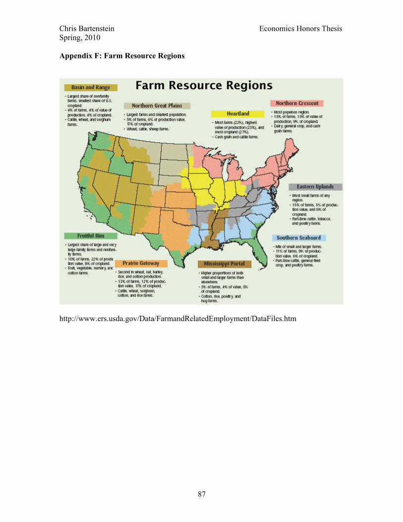
Chris Bartenstein Economics Honors Thesis Spring, 2010
87
Appendix F: Farm Resource Regions
http://www.ers.usda.gov/Data/FarmandRelatedEmployment/DataFiles.htm
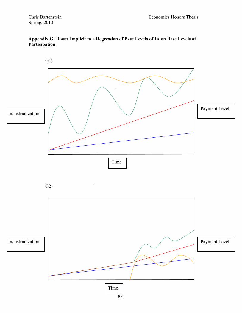
Chris Bartenstein Economics Honors Thesis Spring, 2010
88
Appendix G: Biases Implicit to a Regression of Base Levels of IA on Base Levels of Participation G1) G2)
Time
Industrialization
Time
Industrialization Payment Level
Payment Level
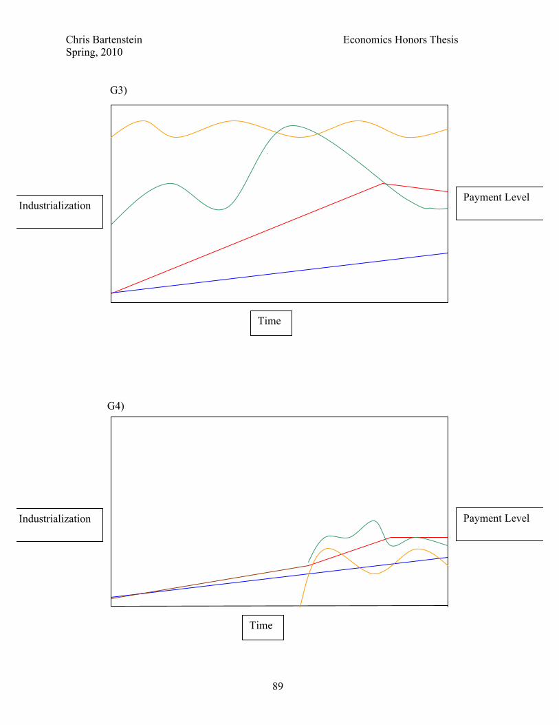
Chris Bartenstein Economics Honors Thesis Spring, 2010
89
G3) G4)
Time
Industrialization Payment Level
Time
Industrialization Payment Level
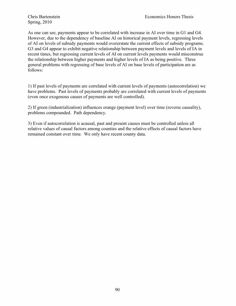
Chris Bartenstein Economics Honors Thesis Spring, 2010
90
As one can see, payments appear to be correlated with increase in AI over time in G1 and G4. However, due to the dependency of baseline AI on historical payment levels, regressing levels of AI on levels of subsidy payments would overerstate the current effects of subsidy programs. G3 and G4 appear to exhibit negative relationship between payment levels and levels of IA in recent times, but regressing current levels of AI on current levels payments would misconstrue the relationship between higher payments and higher levels of IA as being positive. Three general problems with regressing of base levels of AI on base levels of participation are as follows: 1) If past levels of payments are correlated with current levels of payments (autocorrelation) we have problems. Past levels of payments probably are correlated with current levels of payments (even once exogenous causes of payments are well controlled). 2) If green (industrialization) influences orange (payment level) over time (reverse causality), problems compounded. Path dependency. 3) Even if autocorrelation is acausal, past and present causes must be controlled unless all relative values of causal factors among counties and the relative effects of causal factors have remained constant over time. We only have recent county data.
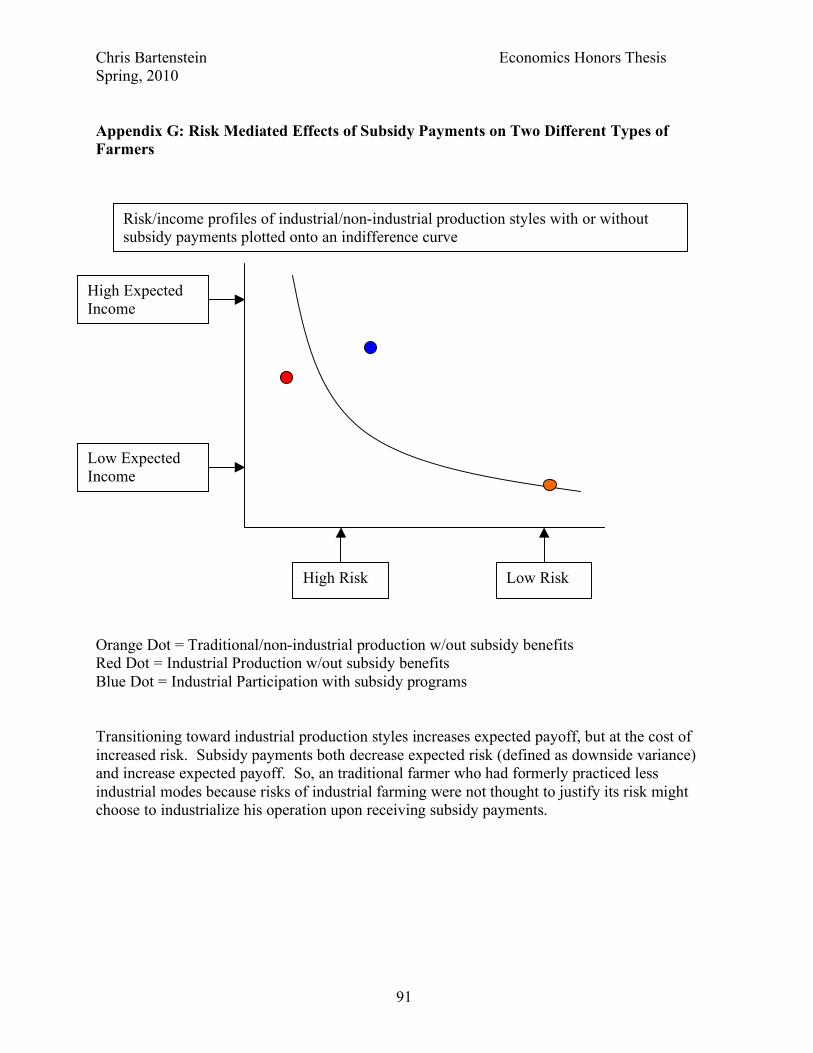
Chris Bartenstein Economics Honors Thesis Spring, 2010
91
Appendix G: Risk Mediated Effects of Subsidy Payments on Two Different Types of Farmers
Orange Dot = Traditional/non-industrial production w/out subsidy benefits Red Dot = Industrial Production w/out subsidy benefits Blue Dot = Industrial Participation with subsidy programs
Transitioning toward industrial production styles increases expected payoff, but at the cost of increased risk. Subsidy payments both decrease expected risk (defined as downside variance) and increase expected payoff. So, an traditional farmer who had formerly practiced less industrial modes because risks of industrial farming were not thought to justify its risk might choose to industrialize his operation upon receiving subsidy payments.
High Expected Income
Low Risk
Low Expected Income
High Risk
Risk/income profiles of industrial/non-industrial production styles with or without subsidy payments plotted onto an indifference curve
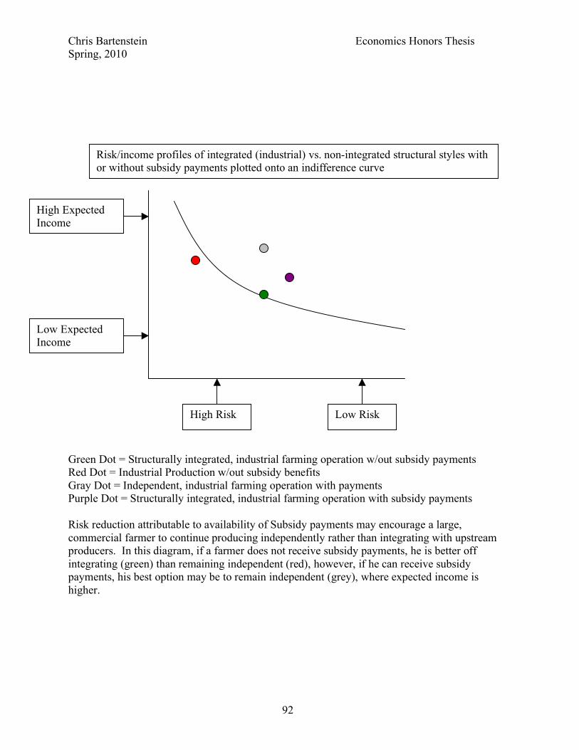
Chris Bartenstein Economics Honors Thesis Spring, 2010
92
Green Dot = Structurally integrated, industrial farming operation w/out subsidy payments Red Dot = Industrial Production w/out subsidy benefits Gray Dot = Independent, industrial farming operation with payments Purple Dot = Structurally integrated, industrial farming operation with subsidy payments Risk reduction attributable to availability of Subsidy payments may encourage a large, commercial farmer to continue producing independently rather than integrating with upstream producers. In this diagram, if a farmer does not receive subsidy payments, he is better off integrating (green) than remaining independent (red), however, if he can receive subsidy payments, his best option may be to remain independent (grey), where expected income is higher.
High Expected Income
Low Risk
Low Expected Income
High Risk
Risk/income profiles of integrated (industrial) vs. non-integrated structural styles with or without subsidy payments plotted onto an indifference curve
Chris Bartenstein Economics Honors Thesis Spring, 2010
93
BIBLIOGRAPHYBabcock, Bruce and Chad Hart, “Risk-Free Farming,” Iowa AG Review, Winter 2004, Vol. 10, No.1. http://www.card.iastate.edu/iowa_ag_review/winter_04/article1.aspx. Beus, Curtis and Riley Dunlap, “Conventional versus Alternative Agriculture: The Paradigmatic Roots of the Debate,” Rural Sociology, 55, No 4, 1990, 590-616. Comer, S.; E. Ekanem, M.; Safdar, S. Singh; and F. Tegegne, “Sustainable and Conventional Farmers: A Comparison of Socio-Economic Characteristics, Attitude, and Beliefs,” Journal of Sustainable Agriculture, Vol. 15, No. 1, 1999, 29-45. Abstract: http://bubl.ac.uk/ARCHIVE/journals/jsusagr/v15n0199.htm Damianos, Dimitri and Dimitri Skuras, “Farm Business and the Development of Alternative Farm Enterprises: An Empirical Analysis in Greece,” Journal of Rural Studies, Vol. 12, Issue 3, July 1996, 273-283. Drabenstott, Dr. Mark, “Forces Driving Industrialization Discussion and Comment,” Industrialization of Heartland Agriculture, Agricultural Economics Miscellaneous Report,No. 176 (Conference Proceedings, July 10-11, 1995, North Dakota State University, Department of Agricultural Economics, Fargo, ND), http://ageconsearch.umn.edu/bitstream/23111/1/aem176.pdf, 21-24. Gliessman, Stephen R., Agroecology: Ecological Processes in Sustainable Agriculture (CRC Press LLC, Boca Raton, Florida, 2000), 3. Stephen R. Gliessman, Agroecology: The Ecology of Sustainable Food Systems, 2nd Edition (CPC Press, Boca Raton, Florida, 2007), 3.AD Halvorson, A. D.; R.L. Anderson; N.E. Toman; and J.R. Welsh, “Economic Comparison for Three Winter Wheat-Fallow Tillage Systems,” Journal of Production Agriculture, Volume 7 (1994), 381–385. Hayami, Yujiro and V. W. Ruttan. "Factor Prices and Technical Change in Agricultural Development: The United States and Japan, 1880-1960," Journal of Political Economy 78 (1970), 1115-141. Hofreither, Markus F.; Erwin Schmid; and Franz Sinabell, “Phasing Out of Environmentally Harmful Subsidies: Consequences of the 2003 CAP Reform,” Prepared for presentation at the American Agricultural Economics Association Annual Meeting, Denver, CO, July 1-4, 2004. ageconsearch.umn.edu/bitstream/20169/1/sp04ho04.pdf. Horowitz, John K. and Erik Lichtenberg, “Insurance, Moral Hazard, and Chemical Use in Agriculture,” American Journal of Agricultural Economics, Vol. 75, No. 4 (Nov., 1993), pp. 926-935.
Chris Bartenstein Economics Honors Thesis Spring, 2010
94
John Ikerd, “Economics of Sustainable Farming,” Presented in the HRM of TX Annual Conference 2001, Systems in Agriculture and Land Management, Fort Worth, TX, March 2-3, 2001. http://web.missouri.edu/~ikerdj/papers/EconomicsofSustainableFarming.htm. Keeney, Dennis and Loni Kemp, A New Agricultural Policy for the United States (The Institute for Agriculture and Trade Policy and The Minnesota Project, July 2003; Produced for the North Atlantic Treaty Organization Advanced Research Workshop on Biodiversity Conservation and Rural Sustainability, Krakow, Poland, November 6, 2002), 11. Lucas, Robert, “Expectations and the Neutrality of Money," Journal of Economic Theory, Vol 4, 103-124. MacCannell, Dean, “Industrial Agriculture and Rural Community Degradation,” Agriculture and Community Change in the U.S. The Concgressional Research Reports (Underview Press, Boulder, CO, 1988), http://www.sarep.ucdavis.edu/newsltr/components/v2n3/sa-4.htm, 15-75 and 325-355. Nail, Elizabeth L.; Douglas L. Young; and William F. Schillinger, “Government Subsidies and Crop Insurance Effects on the Economics of Conservation Cropping Systems in Eastern Washington,” Agronomy Journal 99 (2009), 614-620. Pollan Michael, “Behind the Organic Industrial Complex,” New York Times Magazine, May 13, 2001. http://www.nytimes.com/2001/05/13/magazine/13ORGANIC.html?pagewanted=1. Pollan, Michael, The Omnivore’s Dilemna (The Penguin Group, NY, NY, 2006). Sonka, Dr. Stephen T., “Forces Driving Industrialization,” Industrialization of Heartland Agriculture, Agricultural Economics Miscellaneous Report,No. 176 (Conference Proceedings, July 10-11, 1995, North Dakota State University, Department of Agricultural Economics, Fargo, ND). http://ageconsearch.umn.edu/bitstream/23111/1/aem176.pdf, 13-20. Tweeten, Luther, Agrigultural Industrialization: For Better or Worst? (Anderson Chair Occasional Paper ESO #2404, Department of Agricultural, Environmental, and Development Economics, The Ohio State University, 1998). http://docs.google.com/viewer?a=v&q=cache:wA4Eq41T73sJ:aede.osu.edu/programs/anderson/papers_old/Agricultural%2520Industrialization--For%2520Better%2520or%2520Worse.pdf+Luther+Tweeten,+Agricultural+Industrialization:+For+Better+or+Worse%3F+%28&hl=en&gl=us&pid=bl&srcid=ADGEESjsu8Jw-hyXPK9DRg-kQgzkjTLcgnsNkq6srCgZF9f-cw8M4yoyewcwTGEGEuWVC8EQOmrg3673g3VM3ouSurz631l3XLDTjaXRWHF6Mq7__PNjvcINuxUGua7FWDfnWvJhiWyl&sig=AHIEtbQc0BK9tyAEGTnSKD0a7gtwZFj-AA.
Chris Bartenstein Economics Honors Thesis Spring, 2010
95
United States Department of Agriculture, The Census of Agriculture, National Agricultural Statistics Service, Census Years: 1997, 2002 and 2007. http://www.agcensus.usda.gov/. United States Department of Agriculture, Economic Research Service, The Economics of Food, Farming, Natural Resources, Rural America. Farm and Farm-Related Data Sets. http://www.ers.usda.gov/Data/FarmandRelatedEmployment/DataFiles.htm. United States Government Accountability Office, Report to Congressional Requesters, “Farm Program Payments are an Important Factor in Landowners’ Decisions to Convert Grassland to Cropland,” Sept. 2007. http://www.google.com/search?hl=en&client=firefox-a&rls=org.mozilla%3Aen-US%3Aofficial&channel=s&q=Government+Accountability+Office%2C+Farm+Program+Payments+are+an+Important+Factor+in+Landowners%E2%80%99+Decisions+to+Convert+Grassland+to+Cropland+60+%282007%29%29.+&btnG=Search&cts=1272289388662&aq=f&aqi=&aql=&oq=&gs_rfai=.