Embed Size (px)
Citation preview

Feed-Forward Neural Networks
主講人 : 虞台文
Content
Introduction Single-Layer Perceptron Networks Learning Rules for Single-Layer Perceptron Networks
– Perceptron Learning Rule– Adaline Leaning Rule -Leaning Rule
Multilayer Perceptron Back Propagation Learning algorithm
Feed-Forward Neural Networks
Introduction

Historical Background
1943 McCulloch and Pitts proposed the first computational models of neuron.
1949 Hebb proposed the first learning rule. 1958 Rosenblatt’s work in perceptrons. 1969 Minsky and Papert’s exposed limitation of th
e theory. 1970s Decade of dormancy for neural networks. 1980-90s Neural network return (self-organization,
back-propagation algorithms, etc)
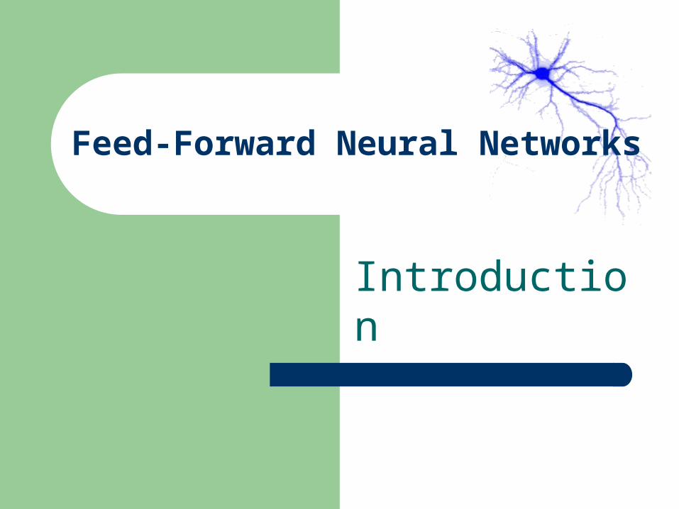
Nervous Systems
Human brain contains ~ 1011 neurons. Each neuron is connected ~ 104 others. Some scientists compared the brain
with a “complex, nonlinear, parallel computer”.
The largest modern neural networks achieve the complexity comparable to a nervous system of a fly.
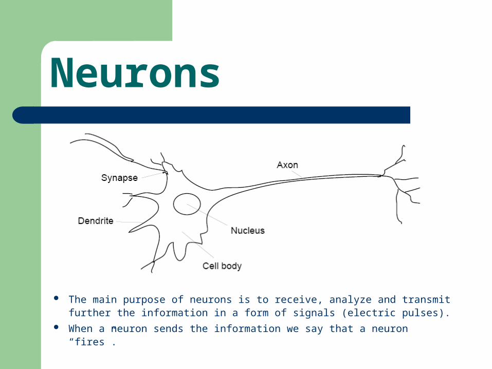
Neurons
The main purpose of neurons is to receive, analyze and transmit further the information in a form of signals (electric pulses).
When a neuron sends the information we say that a neuron “fires”.
Neurons
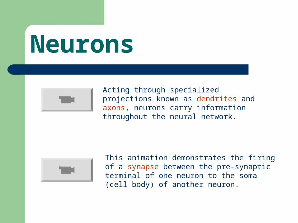
This animation demonstrates the firing of a synapse between the pre-synaptic terminal of one neuron to the soma (cell body) of another neuron.
Acting through specialized projections known as dendrites and axons, neurons carry information throughout the neural network.
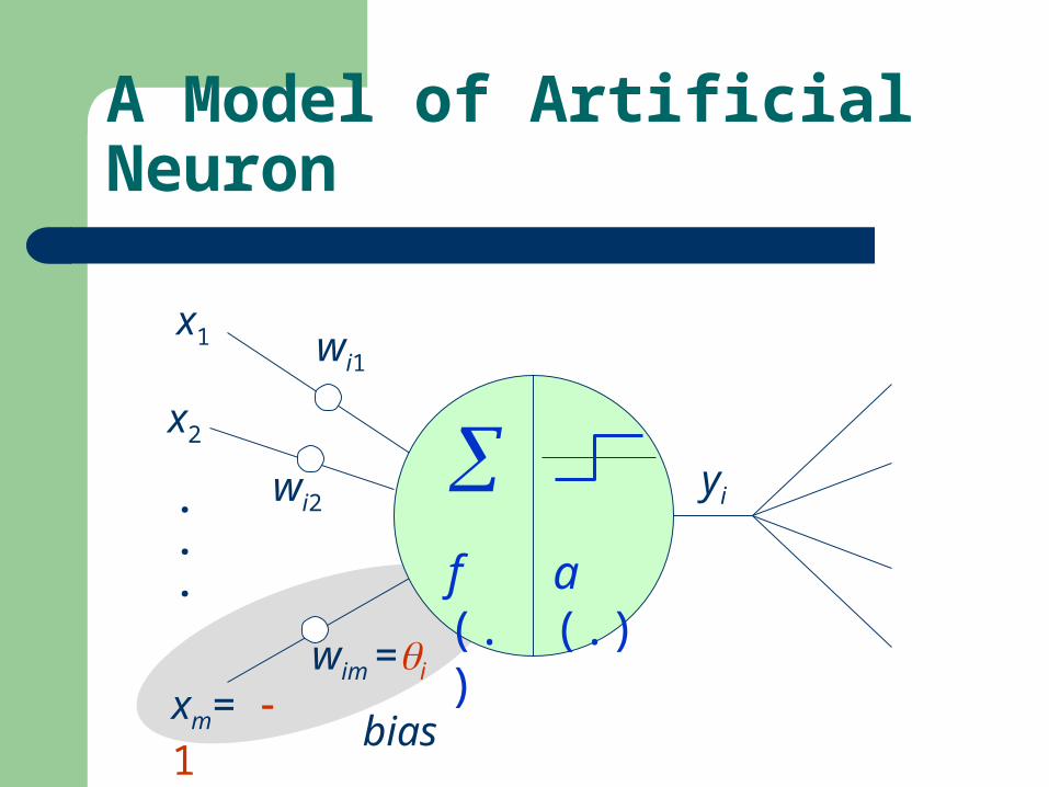
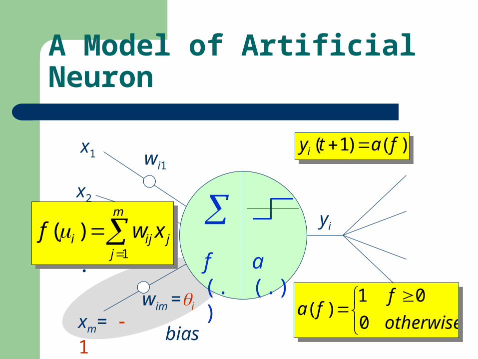
bias
x1
x2
xm= 1
wi1
wi2
wim =i
.
.
.
A Model of Artificial Neuron
yi
f (.) a (.)
bias
x1
x2
xm= 1
wi1
wi2
wim =i
.
.
.
A Model of Artificial Neuron
yi
f (.) a (.)
1
( )m
i ij jj
f w x
1
( )m
i ij jj
f w x
)()1( fatyi )()1( fatyi
otherwise
ffa
0
01)(
otherwise
ffa
0
01)(

Feed-Forward Neural Networks
Graph representation:– nodes: neurons– arrows: signal flow directions
A neural network that does not contain cycles (feedback loops) is called a feed–forward network (or perceptron).
. . .
. . .
. . .
. . .
x1 x2 xm
y1 y2 yn
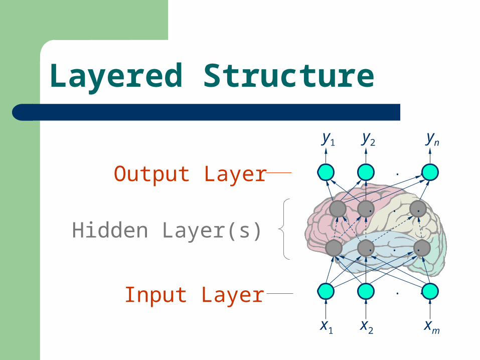
Hidden Layer(s)
Input Layer
Output Layer
Layered Structure
. . .
. . .
. . .
. . .
x1 x2 xm
y1 y2 yn
Knowledge and Memory
. . .
. . .
. . .
. . .
x1 x2 xm
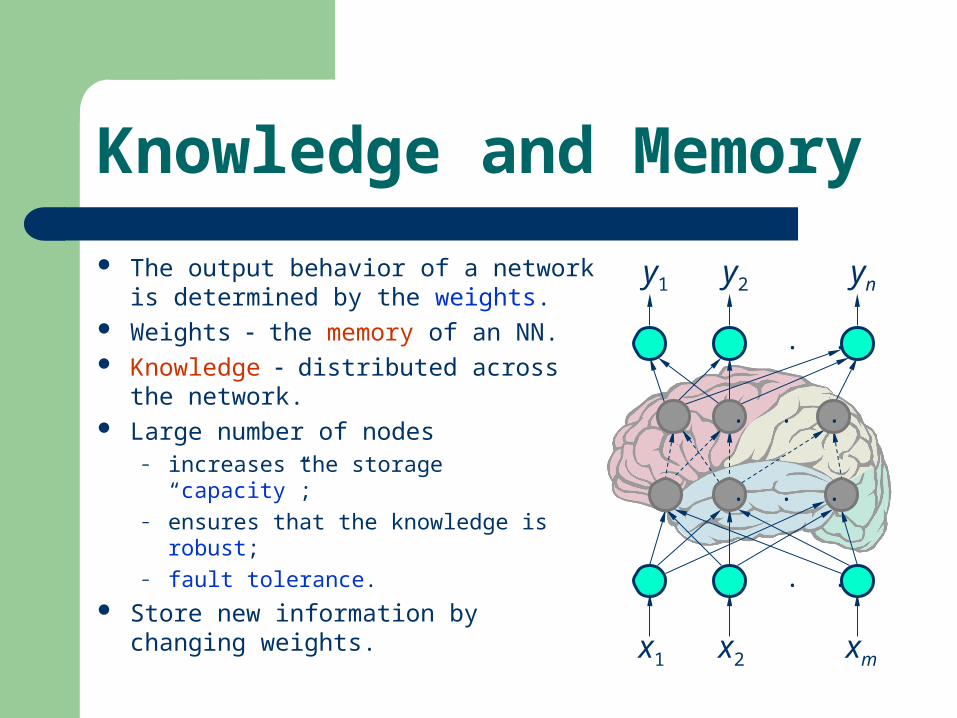
y1 y2 yn The output behavior of a network
is determined by the weights. Weights the memory of an NN. Knowledge distributed across the
network. Large number of nodes
– increases the storage “capacity”;– ensures that the knowledge is
robust;– fault tolerance.
Store new information by changing weights.

Pattern Classification
. . .
. . .
. . .
. . .
x1 x2 xm
y1 y2 yn Function: x y
The NN’s output is used to distinguish between and recognize different input patterns.
Different output patterns correspond to particular classes of input patterns.
Networks with hidden layers can be used for solving more complex problems then just a linear pattern classification.
input pattern xinput pattern x
output pattern youtput pattern y

Training
. . .
. . .
. . .
. . .
(1) (2)(1) (2 )) ( )(( , ), ( , ), , ( , ),kk d d dx xT x
( )1 2( , , , )i
i i imx x xx ( )
1 2( , , , )ii i ind d d d
xi1 xi2 xim
yi1 yi2 yin
Training Set
di1 di2 din
Goal:( ( ))(M )in i
i
iE error dy
( ) 2( )i
i
i dy
Generalization
. . .
. . .
. . .
. . .
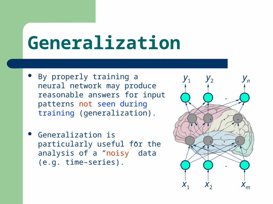
x1 x2 xm
y1 y2 yn By properly training a neural
network may produce reasonable answers for input patterns not seen during training (generalization).
Generalization is particularly useful for the analysis of a “noisy” data (e.g. time–series).

Generalization
. . .
. . .
. . .
. . .
x1 x2 xm
y1 y2 yn By properly training a neural
network may produce reasonable answers for input patterns not seen during training (generalization).
Generalization is particularly useful for the analysis of a “noisy” data (e.g. time–series).
-1.5
-1
-0.5
0
0.5
1
1.5
-1.5
-1
-0.5
0
0.5
1
1.5without noise with noise
Applications
Pattern classificationObject recognitionFunction approximationData compressionTime series analysis and forecast . . .
Feed-Forward Neural Networks
Single-Layer Perceptron Networks
The Single-Layered Perceptron
. . .
x1 x2 xm= 1
y1 y2 yn
xm-1
. . .
. . .
w11w12
w1m
w21
w22
w2m wn1
wnmwn2
Training a Single-Layered Perceptron
. . .
x1 x2 xm= 1
y1 y2 yn
xm-1
. . .
. . .
w11w12
w1m
w21
w22
w2m wn1
wnmwn2
d1 d2 dn
(1) ((1) (2) ))2) ((( , ), ( , ), , ( , )p p x xd d dxT Training Set
Goal:
( )kiy
( )
1
mk
ll
il xwa
1,2, ,
1, 2, ,
i n
k p
( )kid
( )( )Ti
ka xw
Learning Rules
. . .
x1 x2 xm= 1
y1 y2 yn
xm-1
. . .
. . .
w11w12
w1m
w21
w22
w2m wn1
wnmwn2
d1 d2 dn
(1) ((1) (2) ))2) ((( , ), ( , ), , ( , )p p x xd d dxT Training Set
Goal:
( )kiy
( )
1
mk
ll
il xwa
1,2, ,
1, 2, ,
i n
k p
( )kid
( )( )Ti
ka xw
Linear Threshold Units (LTUs) : Perceptron Learning Rule Linearly Graded Units (LGUs) : Widrow-Hoff learning Rule
Feed-Forward Neural Networks
Learning Rules for Single-Layered Perceptron Networks Perceptron Learning Rule Adline Leaning Rule -Learning Rule
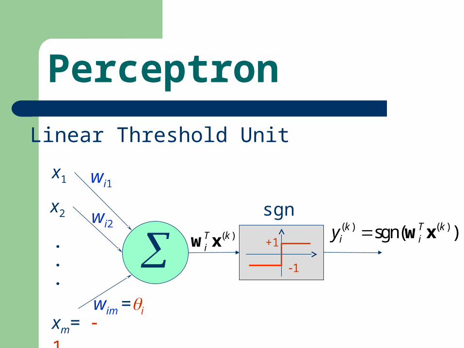
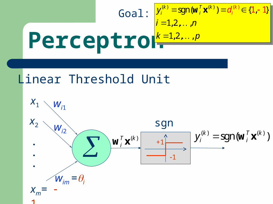
Perceptron
Linear Threshold Unit
( )T kiw x
sgn( ) ( )sgn( )k T ki iy w x
x1
x2
xm= 1
wi1
wi2
wim =i
.
.
. +1
1
Perceptron
Linear Threshold Unit
( )T kiw x
sgn( ) ( )sgn( )k T ki iy w x
) (( ) ( )sgn( ) { , }
1,2, ,
1, 2, ,
1 1ki
k T ki iy
i n
k p
d
w x
) (( ) ( )sgn( ) { , }
1,2, ,
1, 2, ,
1 1ki
k T ki iy
i n
k p
d
w x
Goal:
x1
x2
xm= 1
wi1
wi2
wim =i
.
.
. +1
1
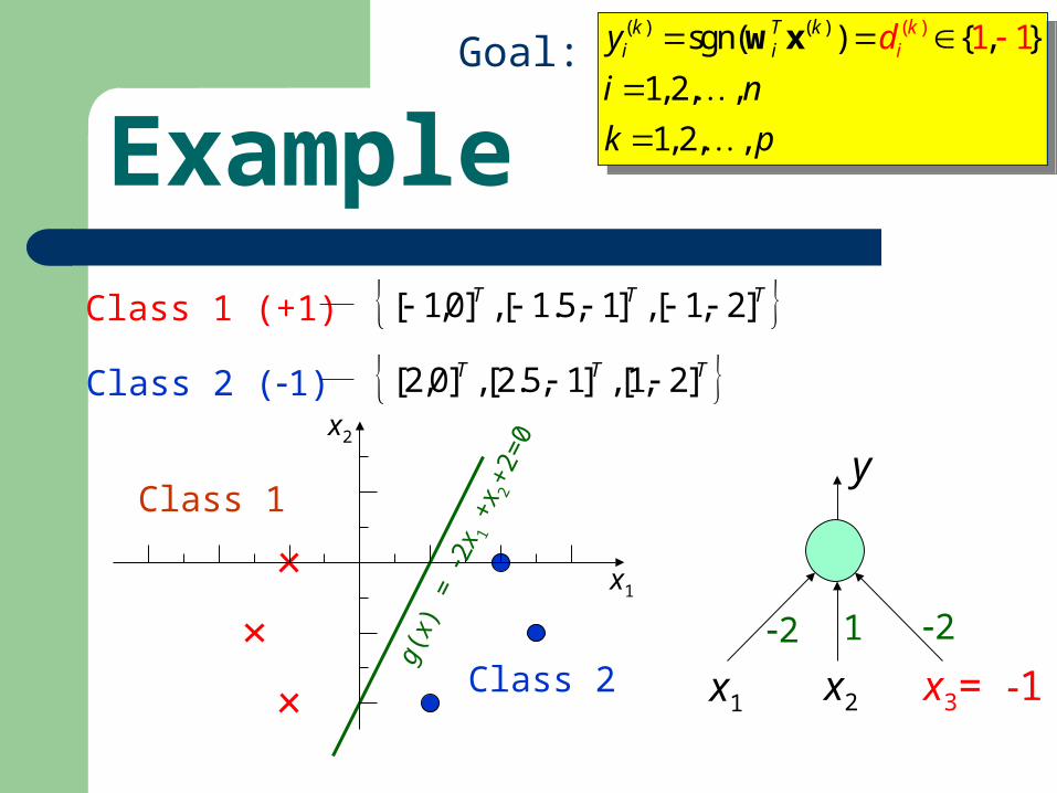
Example
x1 x2 x3= 1
2 1 2
y
TTT ]2,1[,]1,5.1[,]0,1[ Class 1 (+1)
TTT ]2,1[,]1,5.2[,]0,2[ Class 2 (1)
Class 1
Class 2
x1
x2g(
x) =
2x 1
+x2+2
=0
) (( ) ( )sgn( ) { , }
1,2, ,
1, 2, ,
1 1ki
k T ki iy
i n
k p
d
w x
) (( ) ( )sgn( ) { , }
1,2, ,
1, 2, ,
1 1ki
k T ki iy
i n
k p
d
w x
Goal:
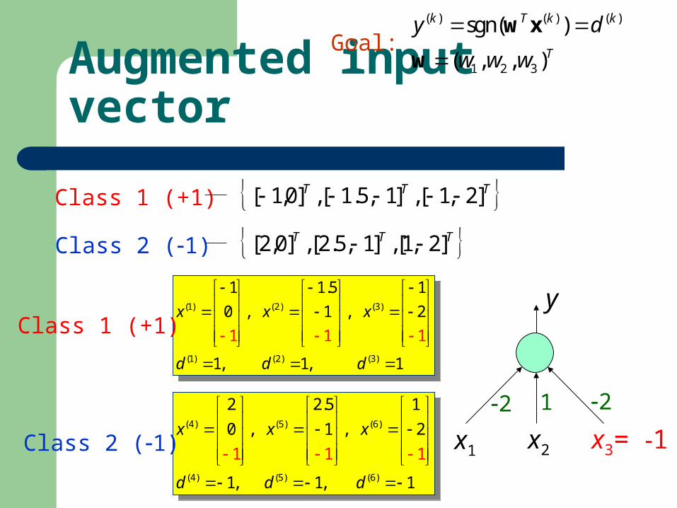
Augmented input vector
x1 x2 x3= 1
2 1 2
y
TTT ]2,1[,]1,5.1[,]0,1[ Class 1 (+1)
TTT ]2,1[,]1,5.2[,]0,2[ Class 2 (1)
(4) (5) (6)
(4) (5) (6)
2 2.5 1
0 , 1 , 2
1, 1, 1
1 1
1
x x x
d d d
(4) (5) (6)
(4) (5) (6)
2 2.5 1
0 , 1 , 2
1, 1, 1
1 1
1
x x x
d d d
(1) (2) (3)
(1) (2) (3)
1 1.5 1
0 , 1 , 2
1, 1,
1 1 1
1
x x x
d d d
(1) (2) (3)
(1) (2) (3)
1 1.5 1
0 , 1 , 2
1, 1,
1 1 1
1
x x x
d d d
Class 1 (+1)
Class 2 (1)
( ) ( ) ( )
1 2 3
sgn( )
( , , )
k T k k
T
y d
w w w
w x
wGoal:
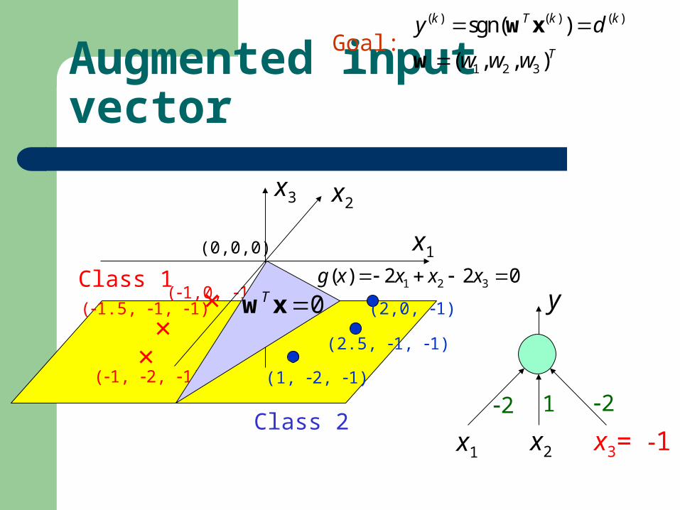
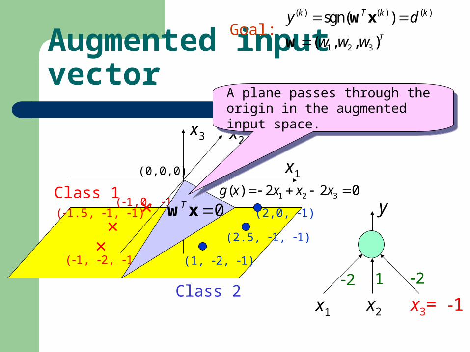
Augmented input vector
x1 x2 x3= 1
2 1 2
yClass 1
(1, 2, 1)
(1.5, 1, 1)(1,0, 1)
Class 2
(1, 2, 1)
(2.5, 1, 1)
(2,0, 1)
x1
x2x3
(0,0,0)
1 2 3( ) 2 2 0g x x x x 0xwT
( ) ( ) ( )
1 2 3
sgn( )
( , , )
k T k k
T
y d
w w w
w x
wGoal:
Augmented input vector
x1 x2 x3= 1
2 1 2
yClass 1
(1, 2, 1)
(1.5, 1, 1)(1,0, 1)
Class 2
(1, 2, 1)
(2.5, 1, 1)
(2,0, 1)
x1
x2x3
(0,0,0)
1 2 3( ) 2 2 0g x x x x 0xwT
( ) ( ) ( )
1 2 3
sgn( )
( , , )
k T k k
T
y d
w w w
w x
wGoal:
A plane passes through the origin in the augmented input space.
A plane passes through the origin in the augmented input space.
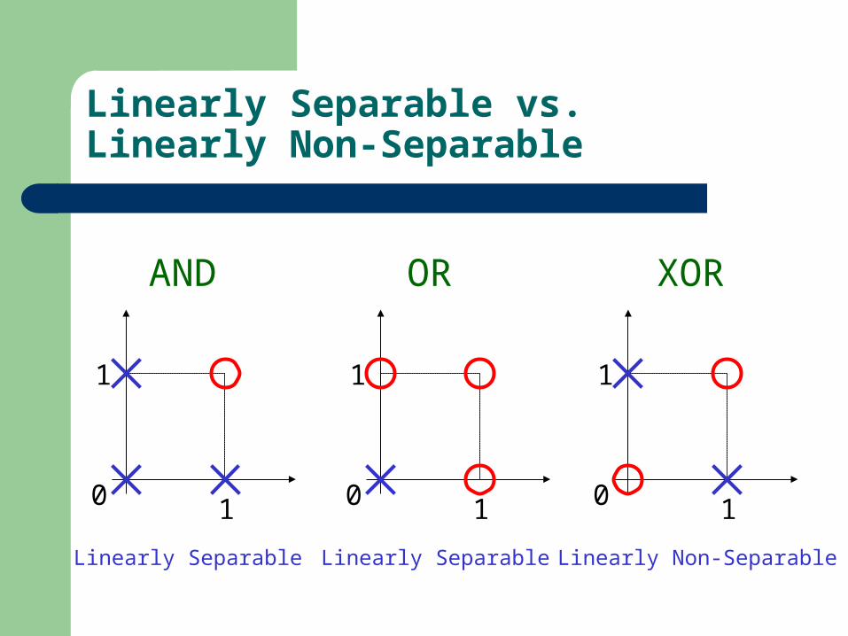
Linearly Separable vs. Linearly Non-Separable
0 1
1
0 1
1
0 1
1
AND OR XOR
Linearly Separable Linearly Separable Linearly Non-Separable
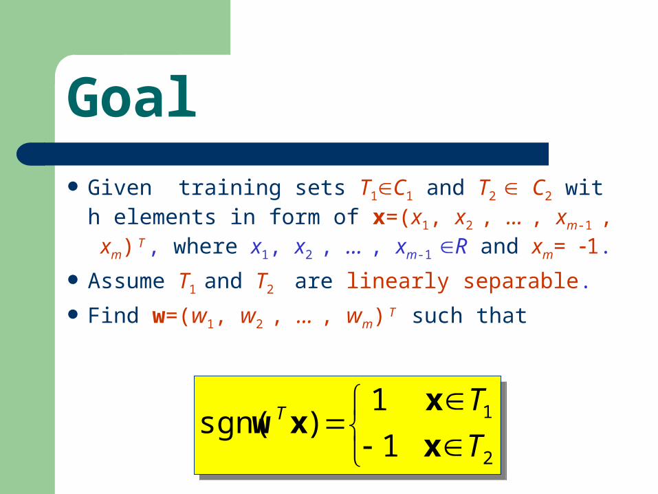
Goal
Given training sets T1C1 and T2 C2 with elements in form of x=(x1, x2 , ... , xm-1 , xm) T , where x1, x2 , ... , xm-1 R and xm= 1.
Assume T1 and T2 are linearly separable. Find w=(w1, w2 , ... , wm) T such that
2
1
1
1)sgn(
T
TT
x
xxw
2
1
1
1)sgn(
T
TT
x
xxw
Goal
Given training sets T1C1 and T2 C2 with elements in form of x=(x1, x2 , ... , xm-1 , xm) T , where x1, x2 , ... , xm-1 R and xm= 1.
Assume T1 and T2 are linearly separable. Find w=(w1, w2 , ... , wm) T such that
2
1
1
1)sgn(
T
TT
x
xxw
2
1
1
1)sgn(
T
TT
x
xxw
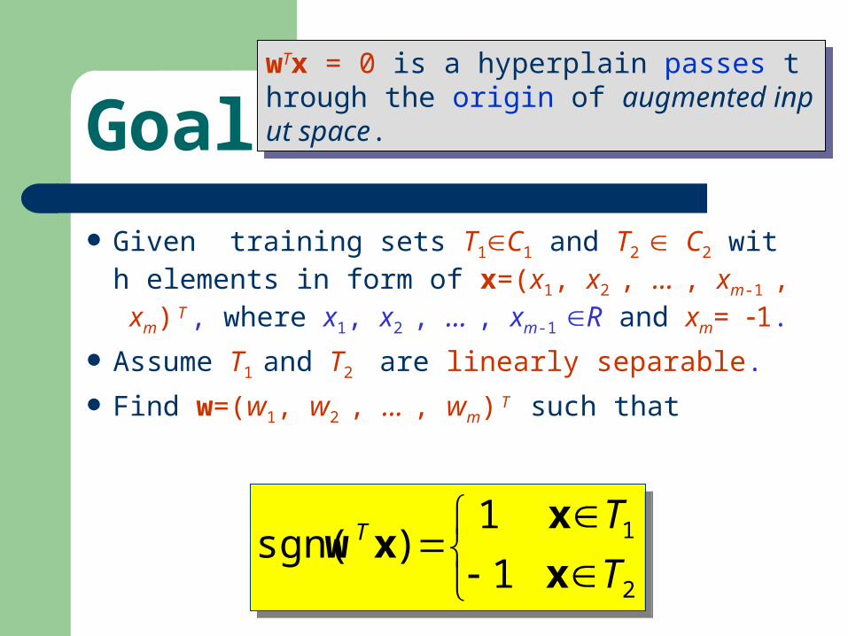
wTx = 0 is a hyperplain passes through the origin of augmented input space.
wTx = 0 is a hyperplain passes through the origin of augmented input space.
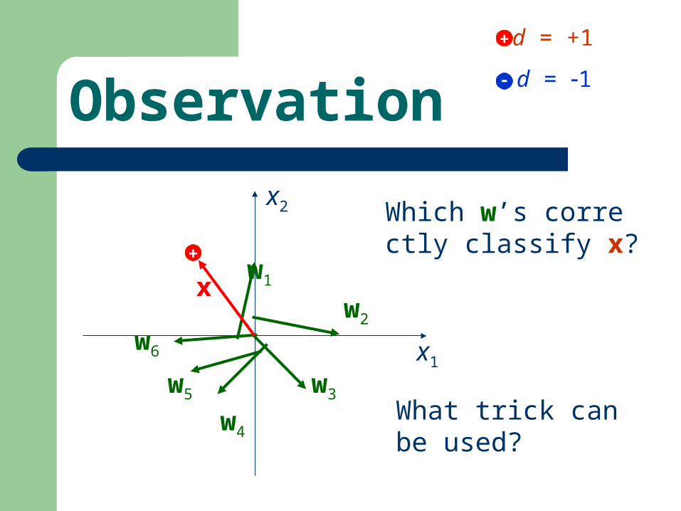
Observation
x1
x2
+
d = +1
d = 1
+w1
w2
w3
w4
w5
w6
x
Which w’s correctly classify x?
What trick can be used?
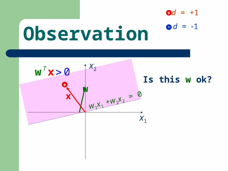
Observation
x1
x2
+
d = +1
d = 1
+
w1x1 +w2x2 = 0w
x
Is this w ok?0T w x
Observation
x1
x2
+
d = +1
d = 1
+
w 1x 1
+w2x 2
= 0
w
x
Is this w ok?0T w x
Observation
x1
x2
+
d = +1
d = 1
+
w 1x 1
+w2x 2
= 0
w
x
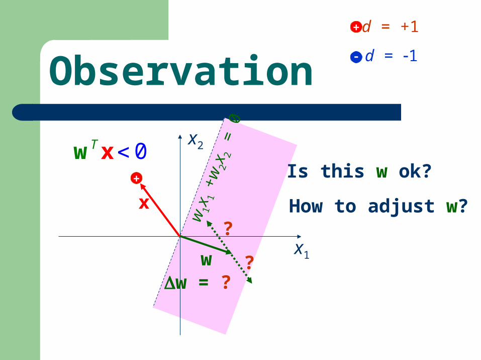
Is this w ok?
How to adjust w?
0T w x
w = ?
?
?

Observation
x1
x2
+
d = +1
d = 1
+
w
x
Is this w ok?
How to adjust w?
0T w x
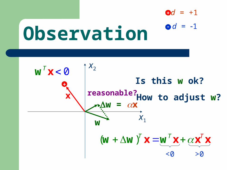
w = x
( )T TT wx xw xw x
reasonable?
<0 >0
Observation
x1
x2
+
d = +1
d = 1
+
w
x
Is this w ok?
How to adjust w?
0T w x
w = x
( )T TT wx xw xw x
reasonable?
<0 >0

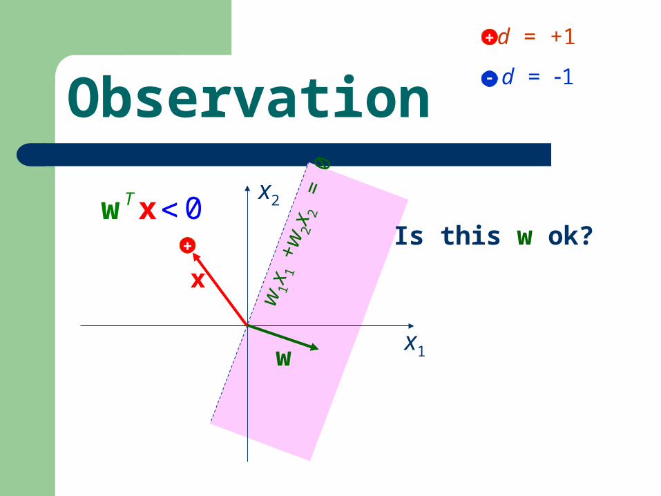
Observation
x1
x2
+
d = +1
d = 1
w
x
Is this w ok?0T w x
w = ?
+x or x
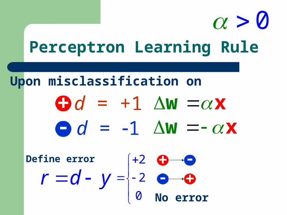
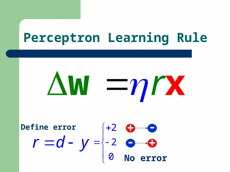
Perceptron Learning Rule
+ d = +1 d = 1
Upon misclassification on
w x w x
Define error
r d y 2
2
0
+ +
No error
0
Perceptron Learning Rule
r w xDefine error
r d y 2
2
0
+ +
No error
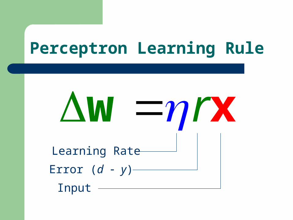
Perceptron Learning Rule
r w xLearning Rate
Error (d y)
Input

Summary Perceptron Learning Rule
Based on the general weight learning rule.
( )( ) i ii x tw t r
ii ir d y
( ( )( )) i i iiw t y td x
0
2 1, 1
2 1, 1
i i
i i
i i
d y
d y
d y
incorrect
correct
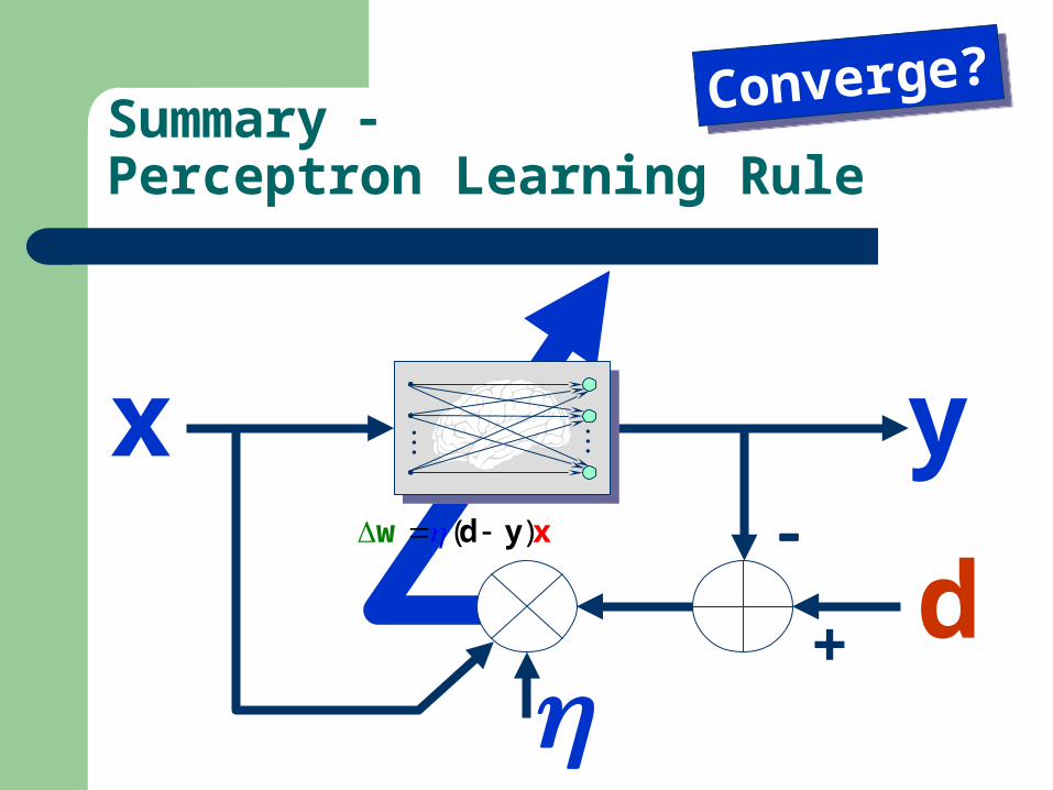
Summary Perceptron Learning Rule
x y( ) d yw x
......
Converge?Converge?
d+
x y( ) d yw x
......
d+
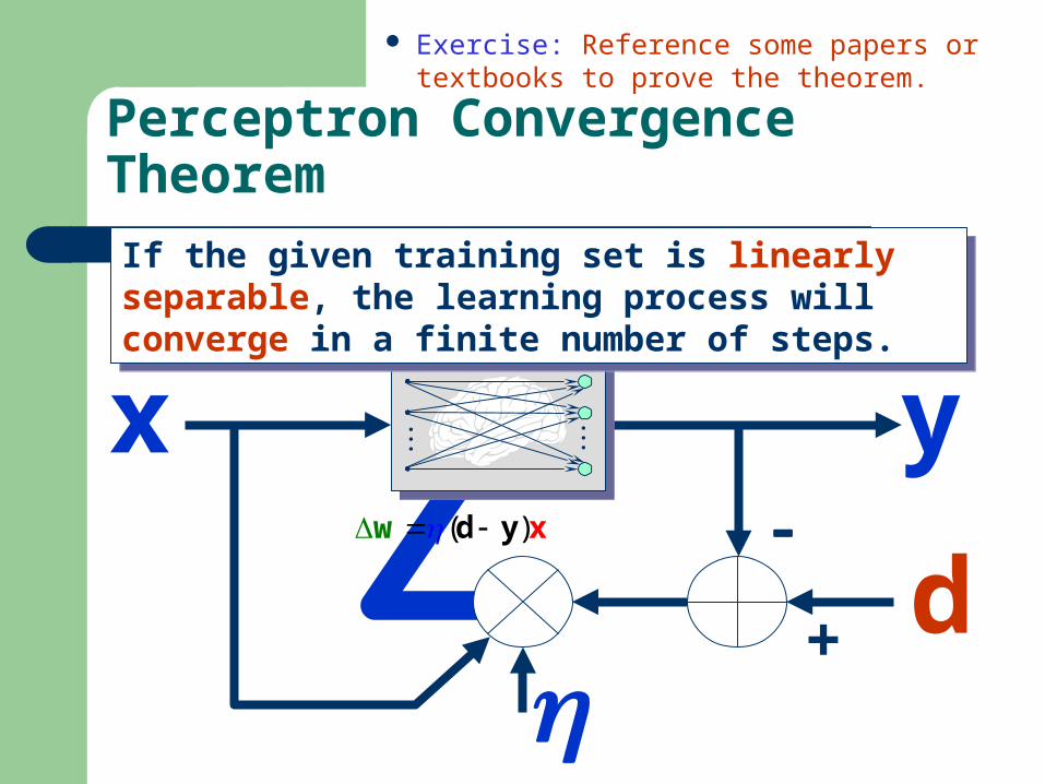
Perceptron Convergence Theorem
Exercise: Reference some papers or textbooks to prove the theorem.
If the given training set is linearly separable, the learning process will converge in a finite number of steps.
If the given training set is linearly separable, the learning process will converge in a finite number of steps.
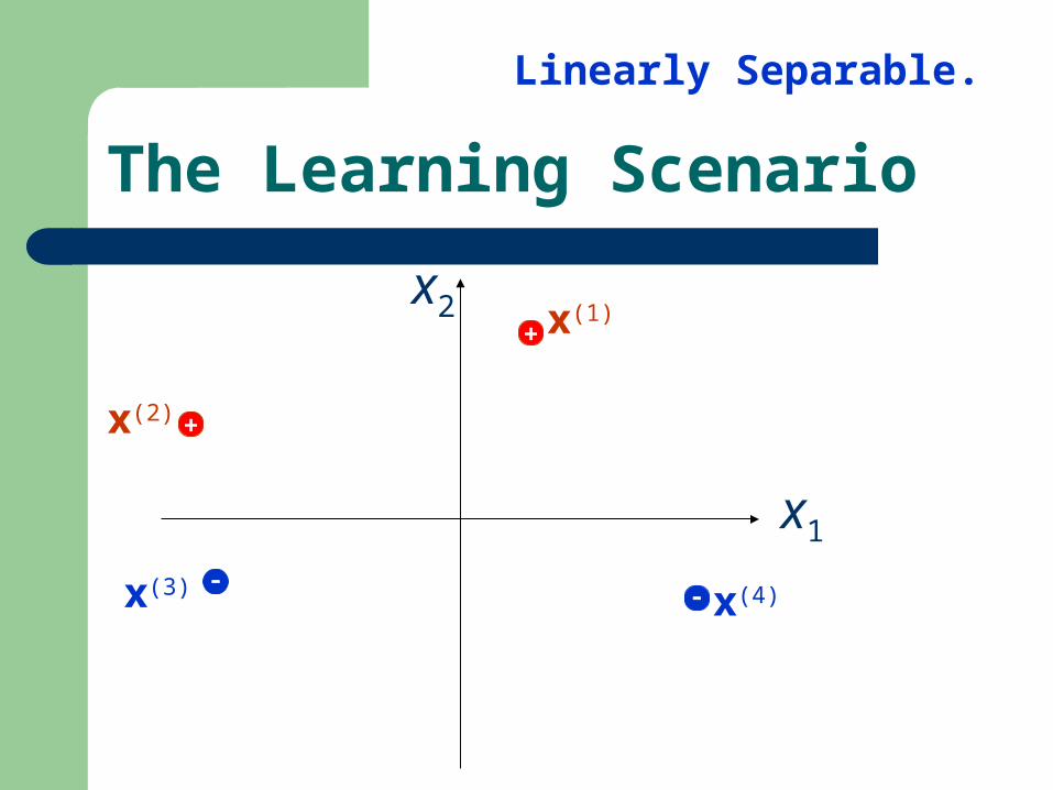
The Learning Scenario
x1
x2+ x(1)
+x(2)
x(3) x(4)
Linearly Separable.
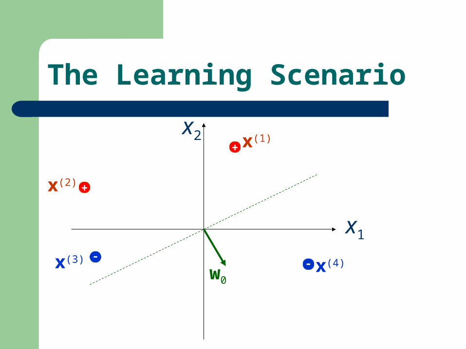
The Learning Scenario
x1
x2
w0
+ x(1)
+x(2)
x(3) x(4)
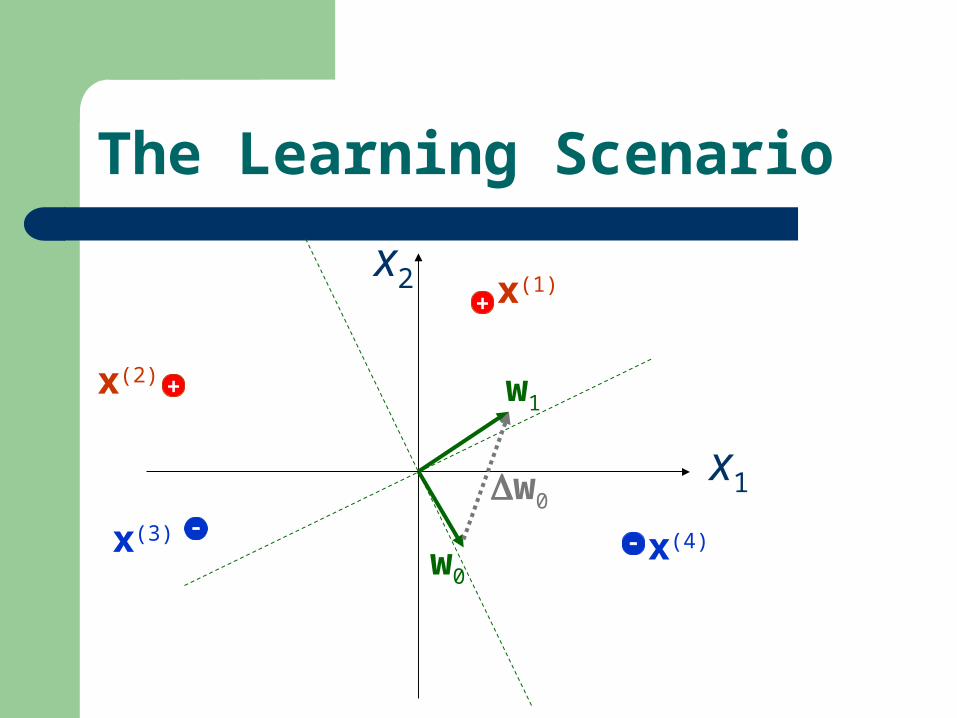
The Learning Scenario
x1
x2
w0
+ x(1)
+x(2)
x(3) x(4)
w1
w0

The Learning Scenario
x1
x2
w0
+ x(1)
+x(2)
x(3) x(4)
w1
w0
w2 w1

The Learning Scenario
x1
x2
w0
+ x(1)
+x(2)
x(3) x(4)
w1
w0
w1
w2
w2 w3
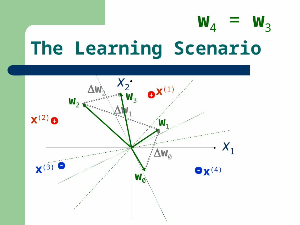
The Learning Scenario
x1
x2
w0
+ x(1)
+x(2)
x(3) x(4)
w1
w0
w1
w2
w2 w3
w4 = w3
The Learning Scenario
x1
x2+ x(1)
+x(2)
x(3) x(4)
w
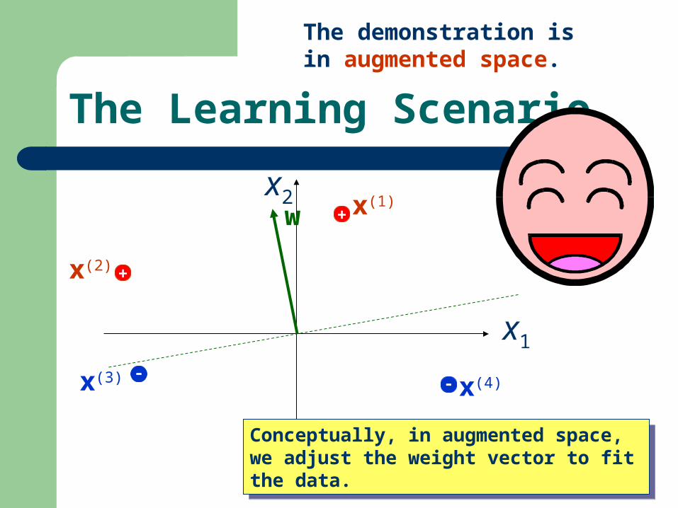
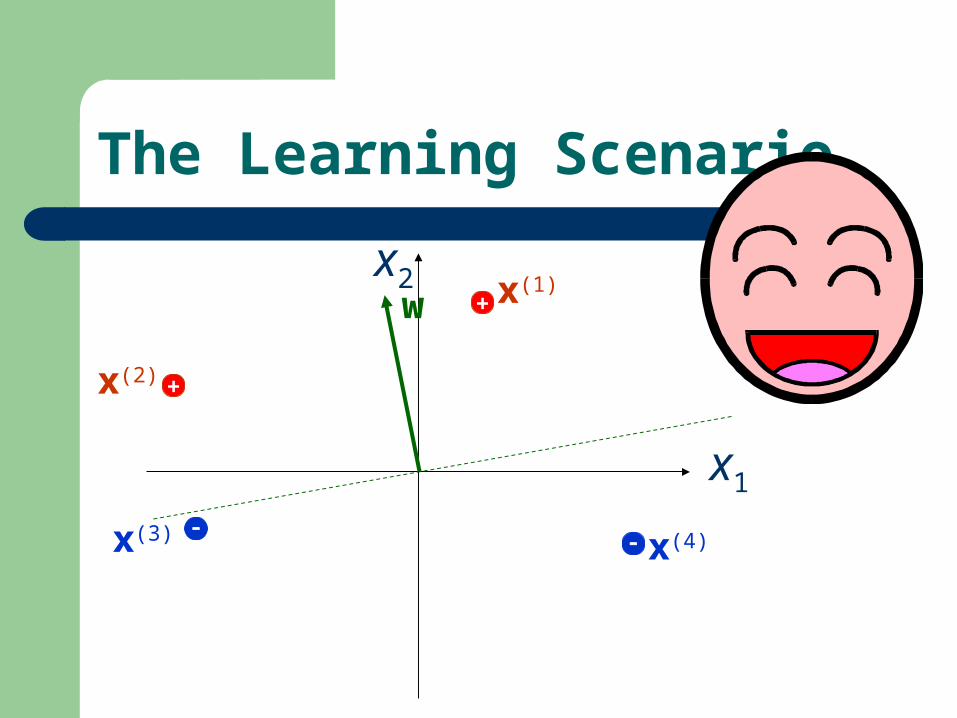
The Learning Scenario
x1
x2+ x(1)
+x(2)
x(3) x(4)
w
The demonstration is in augmented space.
Conceptually, in augmented space, we adjust the weight vector to fit the data.
Conceptually, in augmented space, we adjust the weight vector to fit the data.

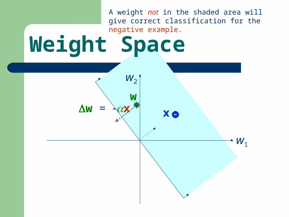
Weight Space
w1
w2
+x
A weight in the shaded area will give correct classification for the positive example.
w
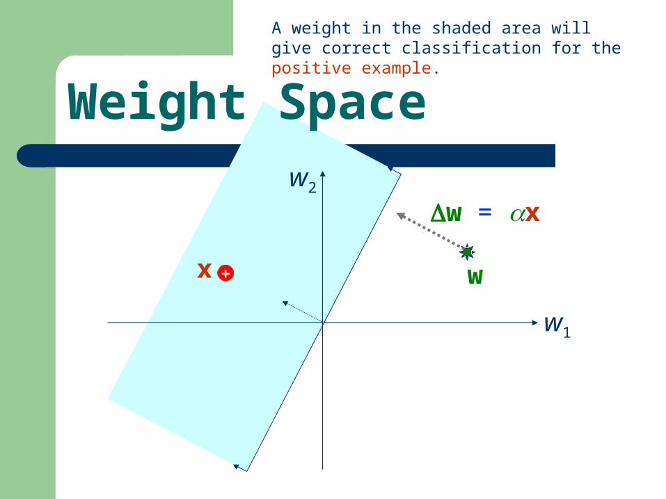
Weight Space
w1
w2
+x
A weight in the shaded area will give correct classification for the positive example.
w
w = x
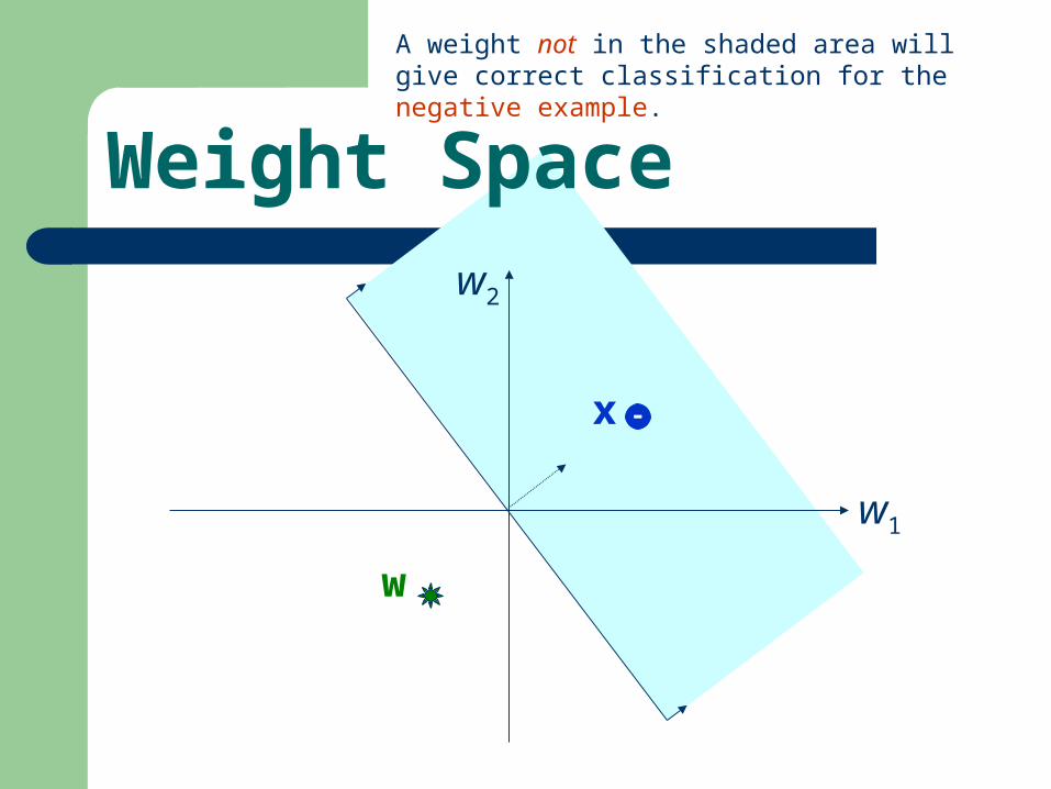
Weight Space
w1
w2
x
A weight not in the shaded area will give correct classification for the negative example.
w
Weight Space
w1
w2
x
A weight not in the shaded area will give correct classification for the negative example.
ww = x
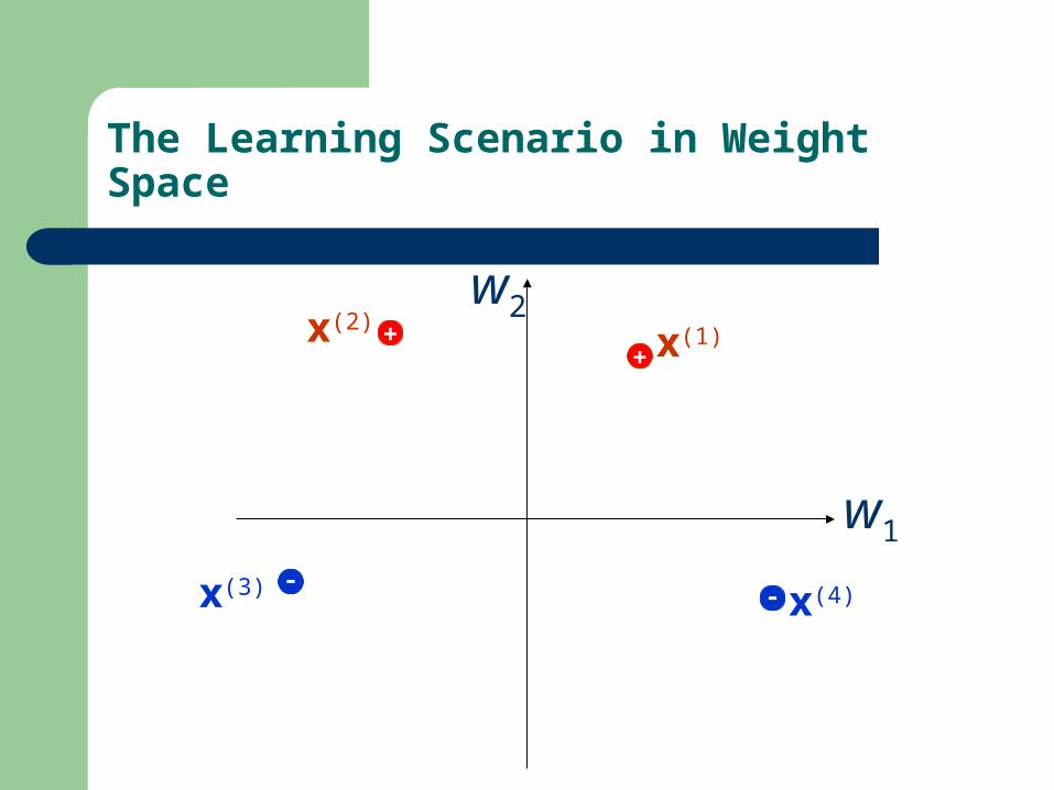
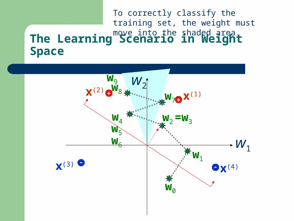
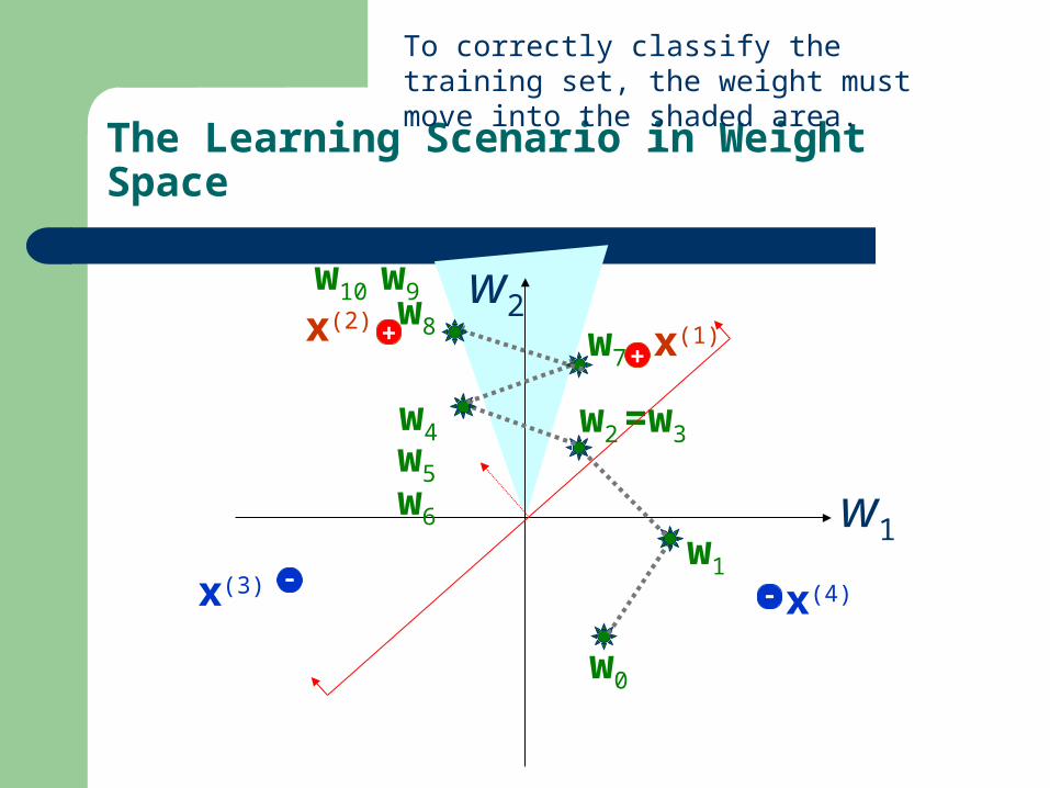
The Learning Scenario in Weight Space
w1
w2
+ x(1)+x(2)
x(3) x(4)

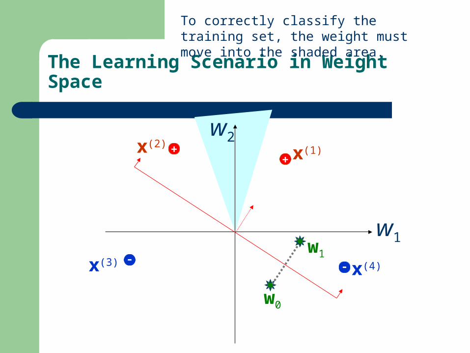
The Learning Scenario in Weight Space
w1
w2
+ x(1)+x(2)
x(3) x(4)
To correctly classify the training set, the weight must move into the shaded area.
The Learning Scenario in Weight Space
w1
w2
+ x(1)+x(2)
x(3) x(4)
To correctly classify the training set, the weight must move into the shaded area.
w0
w1

The Learning Scenario in Weight Space
w1
w2
+ x(1)+x(2)
x(3) x(4)
To correctly classify the training set, the weight must move into the shaded area.
w0
w1
w2
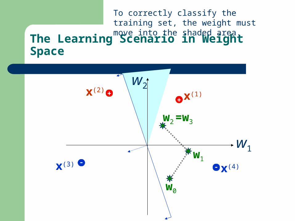
The Learning Scenario in Weight Space
w1
w2
+ x(1)+x(2)
x(3) x(4)
To correctly classify the training set, the weight must move into the shaded area.
w0
w1
w2=w3
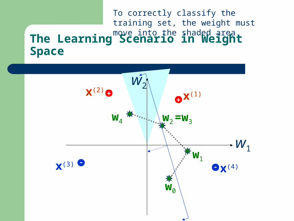
The Learning Scenario in Weight Space
w1
w2
+ x(1)+x(2)
x(3) x(4)
To correctly classify the training set, the weight must move into the shaded area.
w0
w1
w2=w3w4
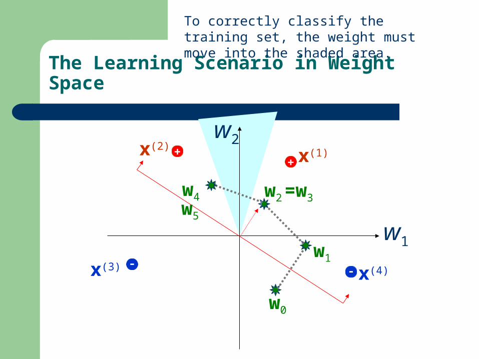
The Learning Scenario in Weight Space
w1
w2
+ x(1)+x(2)
x(3) x(4)
To correctly classify the training set, the weight must move into the shaded area.
w0
w1
w2=w3w4w5
The Learning Scenario in Weight Space
w1
w2
+ x(1)+x(2)
x(3) x(4)
To correctly classify the training set, the weight must move into the shaded area.
w0
w1
w2=w3w4w5
w6

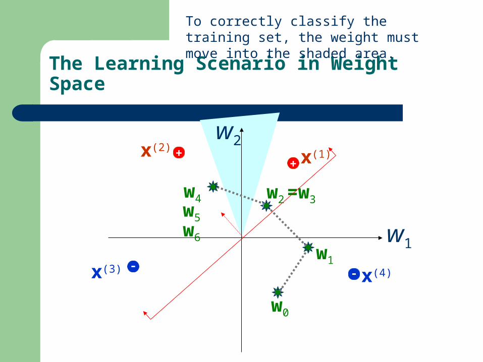
The Learning Scenario in Weight Space
w1
w2
+ x(1)+x(2)
x(3) x(4)
To correctly classify the training set, the weight must move into the shaded area.
w0
w1
w2=w3w4w5
w6
w7
The Learning Scenario in Weight Space
w1
w2
+ x(1)+x(2)
x(3) x(4)
To correctly classify the training set, the weight must move into the shaded area.
w0
w1
w2=w3w4w5
w6
w7
w8
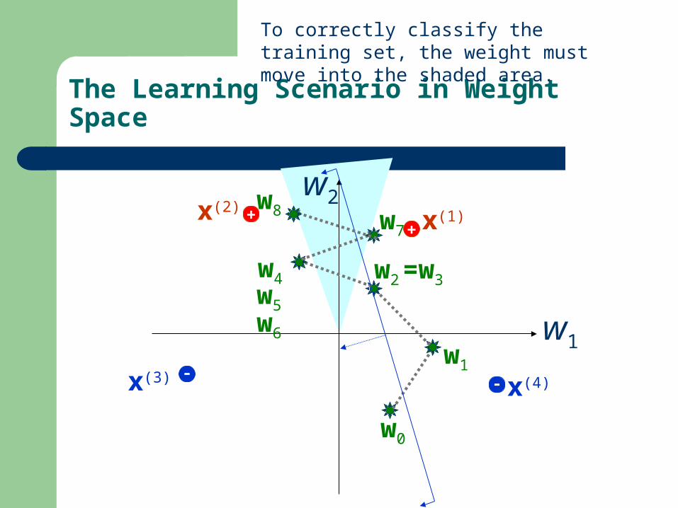
The Learning Scenario in Weight Space
w1
w2
+ x(1)+x(2)
x(3) x(4)
To correctly classify the training set, the weight must move into the shaded area.
w0
w1
w2=w3w4w5
w6
w7
w8
w9
The Learning Scenario in Weight Space
w1
w2
+ x(1)+x(2)
x(3) x(4)
To correctly classify the training set, the weight must move into the shaded area.
w0
w1
w2=w3w4w5
w6
w7
w8
w9w10
The Learning Scenario in Weight Space
w1
w2
+ x(1)+x(2)
x(3) x(4)
To correctly classify the training set, the weight must move into the shaded area.
w0
w1
w2=w3w4w5
w6
w7
w8
w9w10 w11
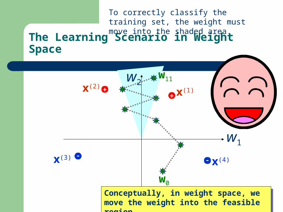
The Learning Scenario in Weight Space
w1
w2
+ x(1)+x(2)
x(3) x(4)
To correctly classify the training set, the weight must move into the shaded area.
w0
w11
Conceptually, in weight space, we move the weight into the feasible region.
Conceptually, in weight space, we move the weight into the feasible region.

Feed-Forward Neural Networks
Learning Rules for Single-Layered Perceptron Networks Perceptron Learning Rule Adaline Leaning Rule -Learning Rule
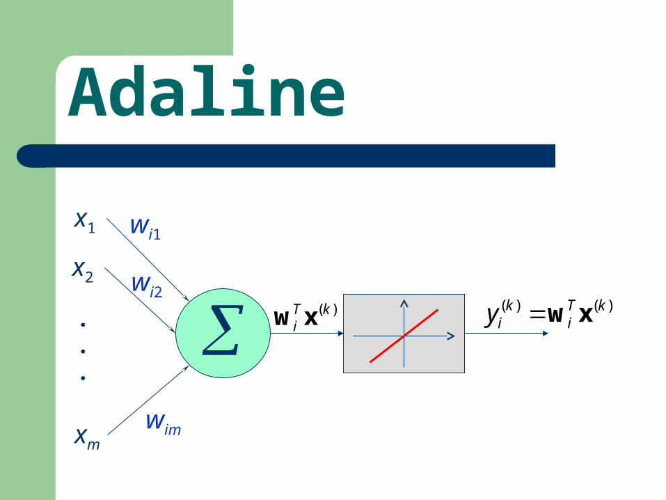
Adaline (Adaptive Linear Element)
Widrow [1962]
( )T kiw x
x1
x2
xm
wi1
wi2
wim
.
.
.
( ) ( )k T ki iy w x
Adaline (Adaptive Linear Element)
Widrow [1962]
( )T kiw x
x1
x2
xm
wi1
wi2
wim
.
.
.
( ) ( )k T ki iy w x
( )( ) ( )
1,2, ,
1, 2, ,
k T k ki i iy
i
d
n
k p
w x
( )( ) ( )
1,2, ,
1, 2, ,
k T k ki i iy
i
d
n
k p
w x
Goal:
In what condition, the goal is reachable?In what condition, the goal is reachable?
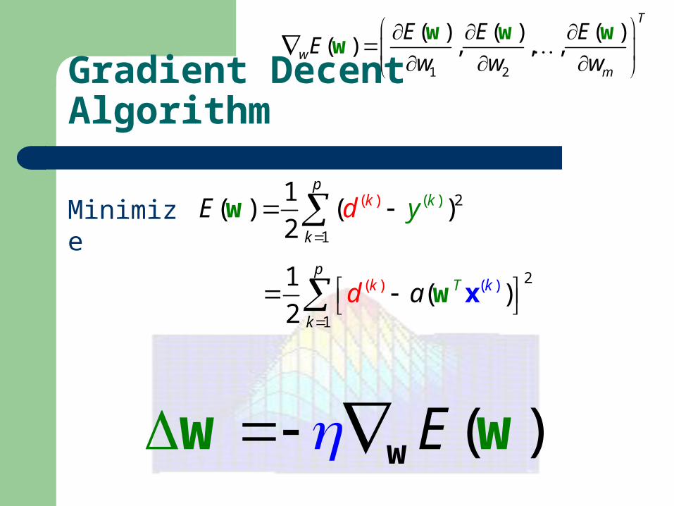
LMS (Least Mean Square)
Minimize the cost function (error function):
( 2
1
( ))1( ) ( )
2k
p
k
kyE d
w
( ( )) 2
1
1( )
2Tk
pk
k
d
xw
( )
1 1
(
2
)1
2
p m
llkk
k l
xwd
Gradient Decent Algorithm
E(w)
w1
w2
Our goal is to go downhill.
Contour Map
(w1, w2) w1
w2w
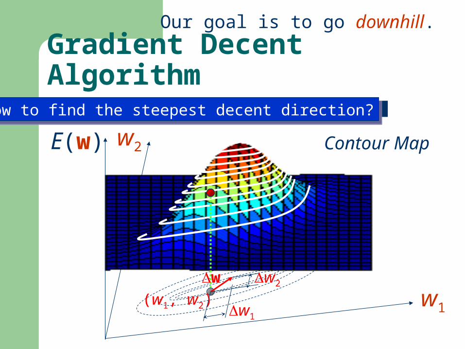
Gradient Decent Algorithm
E(w)
w1
w2
Our goal is to go downhill.
Contour Map
(w1, w2) w1
w2w
How to find the steepest decent direction?How to find the steepest decent direction?
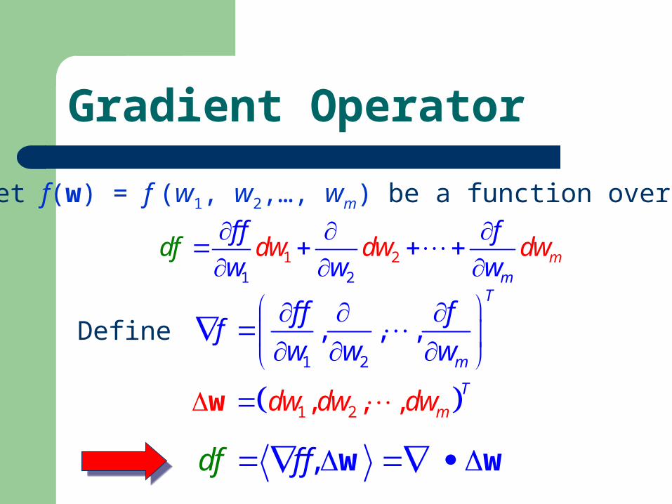
Gradient Operator
Let f(w) = f (w1, w2,…, wm) be a function over Rm.
1 21 2 m
m
f f f
w wdw dwdf w
wd
Define
1 2, , ,T
mdw dw dww
,df f f w w
1 2
, , ,T
m
f f ff
w w w
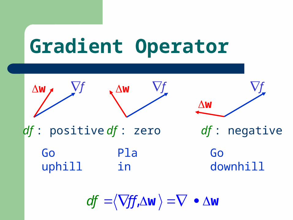
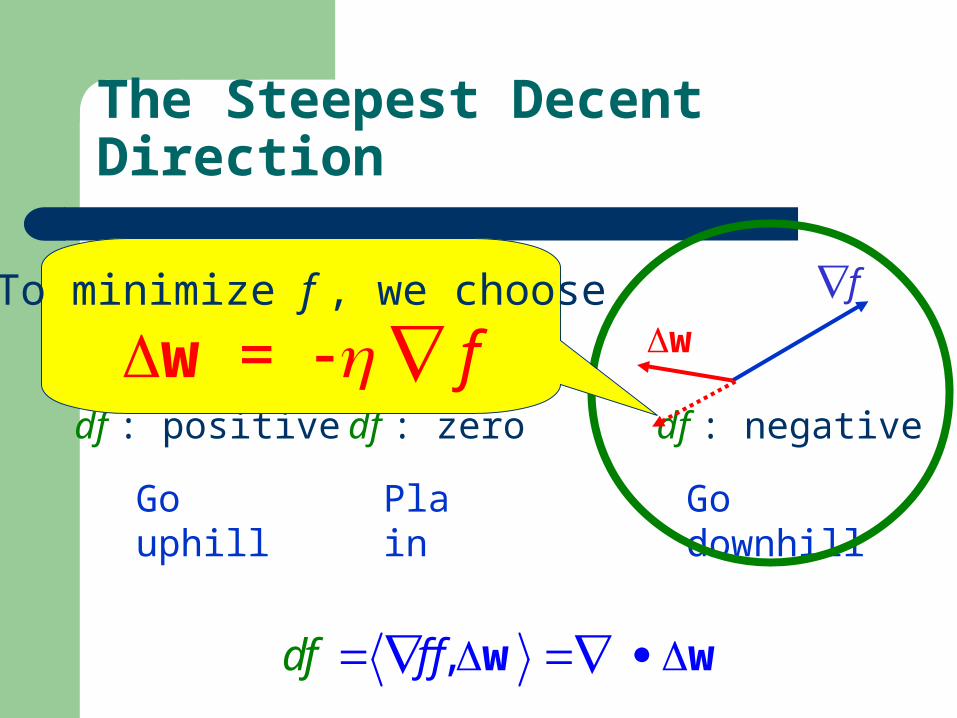
Gradient Operator
fw fw f
w
df : positive df : zero df : negative
Go uphill
Plain
Go downhill
,df f f w w
fw fw f
w
The Steepest Decent Direction
df : positive df : zero df : negative
Go uphill
Plain
Go downhill
,df f f w w
To minimize f , we choose
w = f

LMS (Least Mean Square)
Minimize the cost function (error function):
( )( )
2
1 1
1( )
2
p m
k ll
kl
kd xE w
w
( )
1
( ) (
1
)( ) p m
k l
k kkl j
jl
E
wwd x x
w
( ( )(
1
) )kkp
T kj
k
xd
xw ( )
1
( )) (p
k
k kj
kyd x
( )
1
()( ) kp
k
k
jj
E
wx
w
(k)
( ) ( ) ( )k k kd y

Adaline Learning Rule
Minimize the cost function (error function):
( )( )
2
1 1
1( )
2
p m
k ll
kl
kd xE w
w
1 2
( ) ( ) ( )( ) , , ,
T
wm
E E EE
w w w
w w ww
( )E ww w Weight Modification Rule
( )
1
()( ) kp
k
k
jj
E
wx
w ( ) ( ) ( )k k kd y

Learning Modes
Batch Learning Mode:
Incremental Learning Mode:
( ( ))
1
p
k
k kjj xw
( ( ))k kjj xw
( )
1
()( ) kp
k
k
jj
E
wx
w ( ) ( ) ( )k k kd y

Summary Adaline Learning Rule
x y w δx
......
d+
-Learning RuleLMS AlgorithmWidrow-Hoff Learning Rule
Converge?Converge?
LMS Convergence
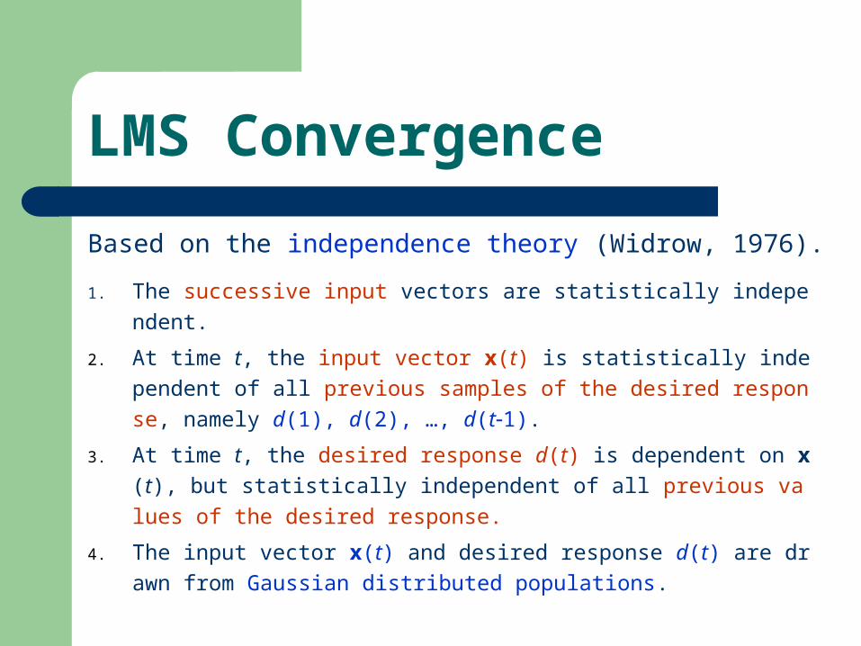
Based on the independence theory (Widrow, 1976).
1. The successive input vectors are statistically independent.2. At time t, the input vector x(t) is statistically independent of a
ll previous samples of the desired response, namely d(1), d(2),
…, d(t1).3. At time t, the desired response d(t) is dependent on x(t), but s
tatistically independent of all previous values of the desired response.
4. The input vector x(t) and desired response d(t) are drawn from Gaussian distributed populations.
LMS Convergence
It can be shown that LMS is convergent if
max
20
where max is the largest eigenvalue of the correlation matrix Rx for the inputs.
1
1lim T
i in
in
xR x x

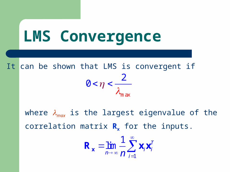
LMS Convergence
It can be shown that LMS is convergent if
max
20
where max is the largest eigenvalue of the correlation matrix Rx for the inputs.
1
1lim T
i in
in
xR x x
Since max is hardly available, we commonly use
20
( )tr
xR
20
( )tr
xR
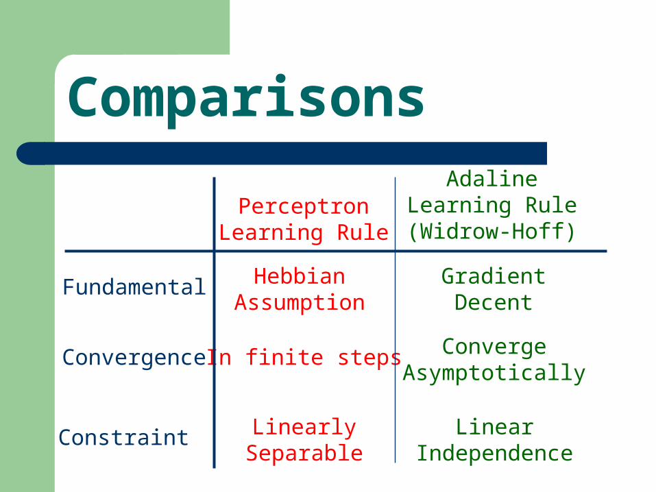
Comparisons
Fundamental HebbianAssumption
GradientDecent
Convergence In finite steps ConvergeAsymptotically
Constraint LinearlySeparable
LinearIndependence
PerceptronLearning Rule
AdalineLearning Rule(Widrow-Hoff)
Feed-Forward Neural Networks
Learning Rules for Single-Layered Perceptron Networks Perceptron Learning Rule Adaline Leaning Rule -Learning Rule
Adaline
( )T kiw x
x1
x2
xm
wi1
wi2
wim
.
.
.
( ) ( )k T ki iy w x
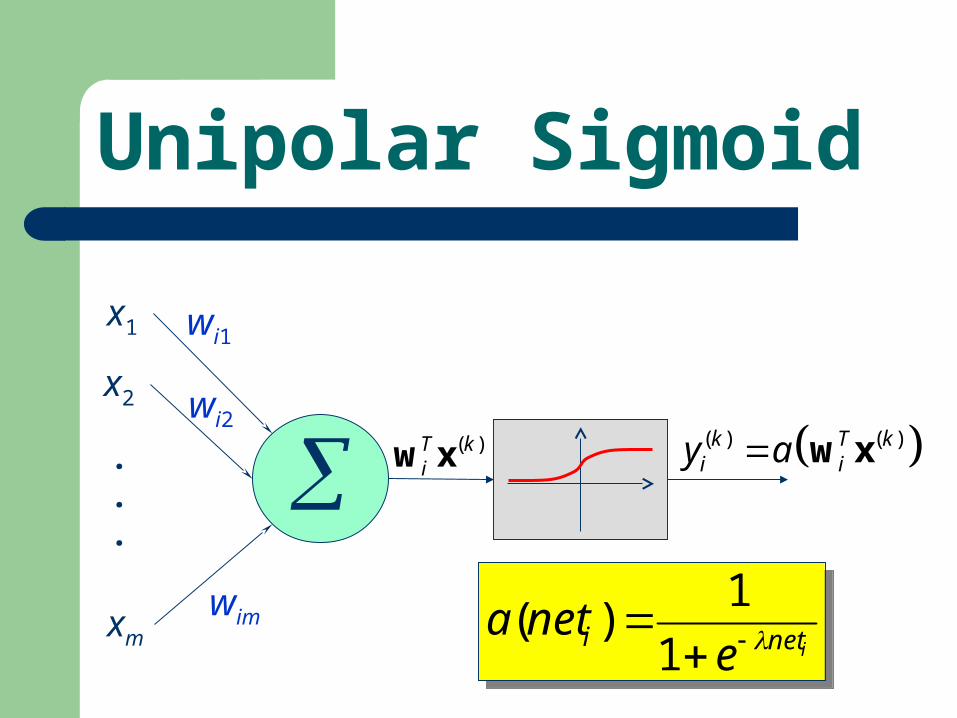
Unipolar Sigmoid
( )T kiw x
x1
x2
xm
wi1
wi2
wim
.
.
.
ineti eneta
1
1)(
ineti eneta
1
1)(
( ) ( )k T ki iy a w x
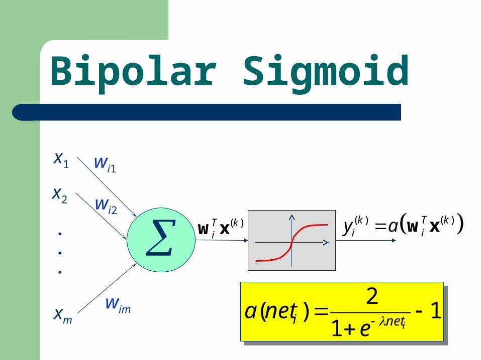
Bipolar Sigmoid
( )T kiw x
x1
x2
xm
wi1
wi2
wim
.
.
. ( ) ( )k T k
i iy a w x
11
2)(
ineti e
neta 1
1
2)(
ineti e
neta
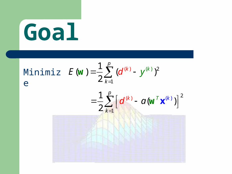
Goal
Minimize
( 2
1
( ))1( ) ( )
2k
p
k
kyE d
w
( 2)
1
( )1( )
2kT
p
k
kd a
w x
Gradient Decent Algorithm
Minimize
( 2
1
( ))1( ) ( )
2k
p
k
kyE d
w
( )E ww w
1 2
( ) ( ) ( )( ) , , ,
T
wm
E E EE
w w w
w w ww
( 2)
1
( )1( )
2kT
p
k
kd a
w x
The Gradient
Minimize
( 2
1
( ))1( ) ( )
2k
p
k
kyE d
w
)( ()k T kay w x )( ()k T kay w x
( )(
1
)( )( )( )
kk
j
p
k j
kdy
yw
E
w
w
1 2
( ) ( ) ( )( ) , , ,
T
wm
E E EE
w w w
w w ww
( )
( ) ( )
(( )
1)
( )k k
k
p
k j
k knet net
nety
w
ad
( ) ( )kTknet xw (
1
)km
iii xw
? ?
( )( )
j
kk
jw
netx
Depends on the activation function
used.
Depends on the activation function
used.
Weight Modification Rule
Minimize
( 2
1
( ))1( ) ( )
2k
p
k
kyE d
w
1
( )
( )
( )(
))
(( )( )
p
k
kkk
jj
k
knetx
aEy
w ned
t
w
1 2
( ) ( ) ( )( ) , , ,
T
wm
E E EE
w w w
w w ww
(( ))k knety a (( ))k knety a
(
1
)
(( )
( ))
k
kkp
kj jk
new
a tx
net
( ) ( ) ( )k k kd y ( ) ( ) ( )k k kd y
Learning Rule
Batch
)
( )
(( )
( )
k
kkj j
knet
net
axw
Incremental

The Learning Efficacy
Minimize
( 2
1
( ))1( ) ( )
2k
p
k
kyE d
w
1 2
( ) ( ) ( )( ) , , ,
T
wm
E E EE
w w w
w w ww
AdalineSigmoid
Unipolar Bipolar
( )neta net1
( )1 net
ae
net
2( ) 1
1 neta n
eet
( )
1a net
net
( ) ( )(1 )
( ) k knet
nety y
a
Exercise
(( ))k knety a (( ))k knety a
1
( )
( )
( )(
))
(( )( )
p
k
kkk
jj
k
knetx
aEy
w ned
t
w
Learning Rule Unipolar Sigmoid
Minimize
( 2
1
( ))1( ) ( )
2k
p
k
kyE d
w
( ) ( ) ( )) ( )
1
( (( ))
1(
)k kj
k kp
kj
k yE
xd y yw
w
1 2
( ) ( ) ( )( ) , , ,
T
wm
E E EE
w w w
w w ww
( ) )) ( (( )
1
(1 )k k k
k
kj
p
y yx
( ) ( ) ( )k k kd y ( ) ( ) ( )k k kd y
( () ) ( )(
1
) (1 )kj
kp
k
k kj xw y y
Weight Modification Rule
( )( )(1 )
kky y
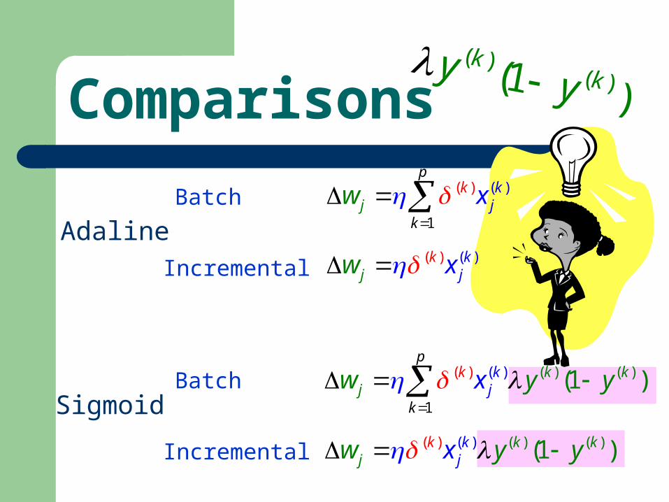
Comparisons
( () ) ( )(
1
) (1 )kj
kp
k
k kj xw y y
Adaline
Sigmoid
Batch
Incremental
( ( ))
1
p
k
kj j
kw x
( ( ))k k
jj xw
Batch
Incremental ( )) ( ) )( ((1 )jkkk k
jw y yx
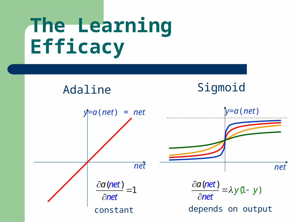
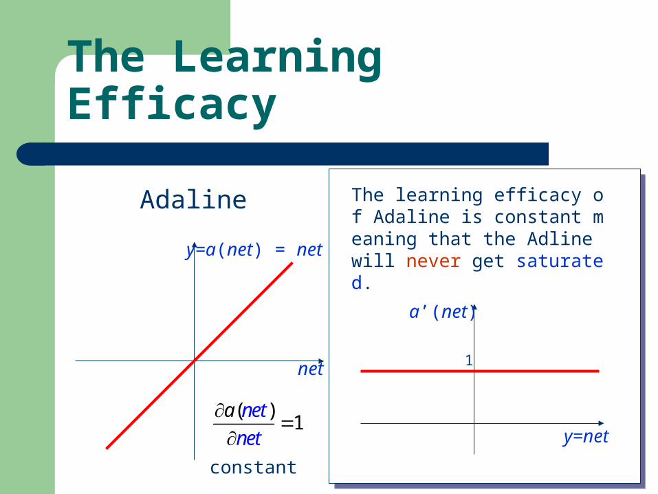
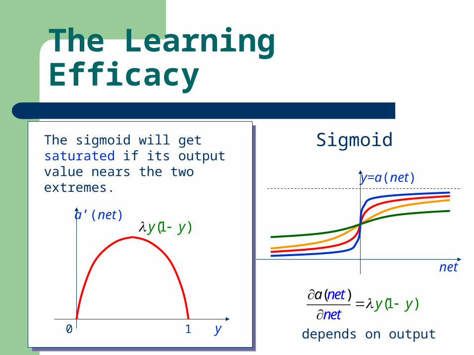
The Learning Efficacy
net
y=a(net) = net
net
y=a(net)
Adaline Sigmoid
( )1
a net
net
)
)(
(1net
ney
a
ty
constant depends on output
The Learning Efficacy
net
y=a(net) = net
net
y=a(net)
Adaline Sigmoid
( )1
a net
net
)
)(
(1net
ney
a
ty
constant depends on output
The learning efficacy of Adaline is constant meaning that the Adline will never get saturated.
y=net
a’(net)
1
The Learning Efficacy
net
y=a(net) = net
net
y=a(net)
Adaline Sigmoid
( )1
a net
net
)
)(
(1net
ney
a
ty
constant depends on output
The sigmoid will get saturated if its output value nears the two extremes.
y
a’(net)
10
(1 )y y
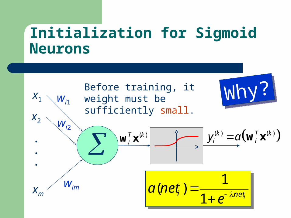
Initialization for Sigmoid Neurons
ineti eneta
1
1)(
ineti eneta
1
1)(
wi1
wi2
wim
x1
x2
xm
.
.
.
( )T kiw x ( ) ( )k T k
i iy a w x
Before training, it weight must be sufficiently small. Why?Why?
Feed-Forward Neural Networks
Multilayer Perceptron
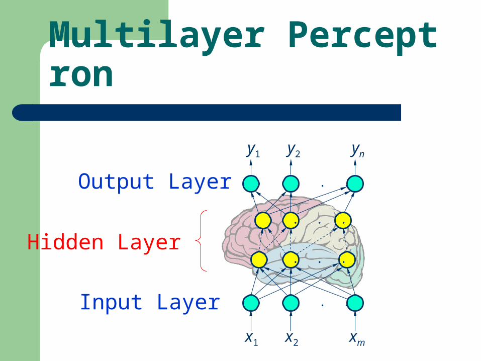
Multilayer Perceptron
. . .
. . .
. . .
. . .
x1 x2 xm
y1 y2 yn
Hidden Layer
Input Layer
Output Layer
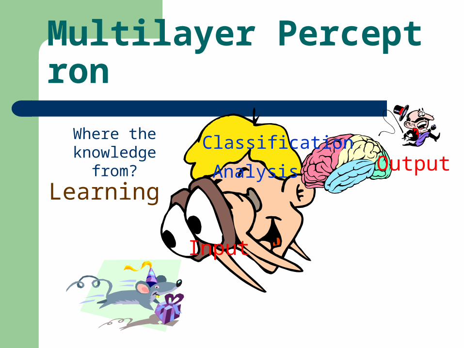
Multilayer Perceptron
Input
Analysis
ClassificationOutput
Learning
Where the knowledge
from?
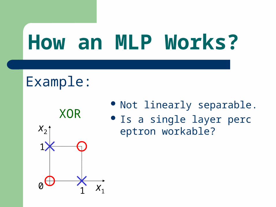
How an MLP Works?
XOR
0 1
1
x1
x2
Example:
Not linearly separable. Is a single layer perceptro
n workable?
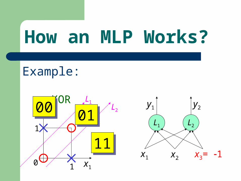
How an MLP Works?
0 1
1
XOR
x1
x2
Example:
L1L20000
0101
1111
L2L1
x1 x2 x3= 1
y1 y2

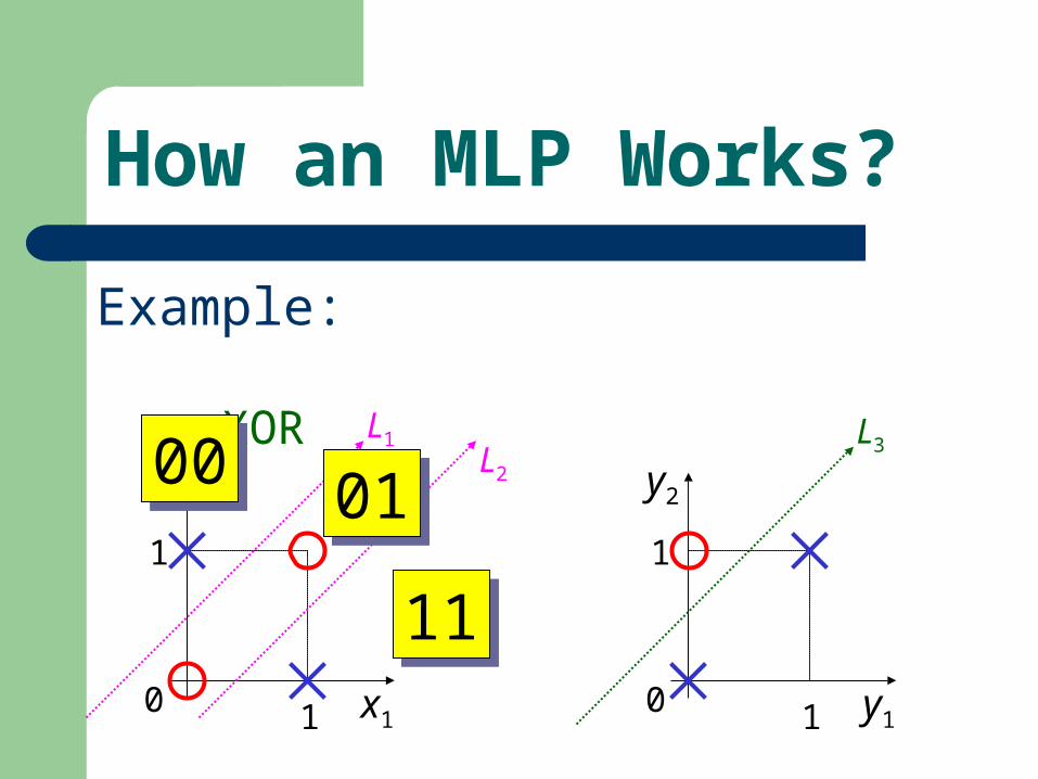
How an MLP Works?
0 1
1
XOR
x1
x2
Example:
L1L20000
0101
11110 1
1
y1
y2
L3
How an MLP Works?
0 1
1
XOR
x1
x2
Example:
L1L20000
0101
11110 1
1
y1
y2
L3
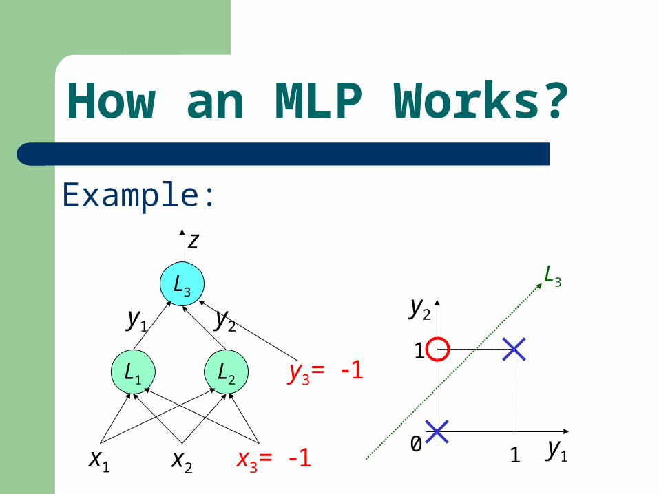
How an MLP Works?
0 1
1
y1
y2
L3
L2L1
x1 x2 x3= 1
L3
y1 y2
y3= 1
z
Example:
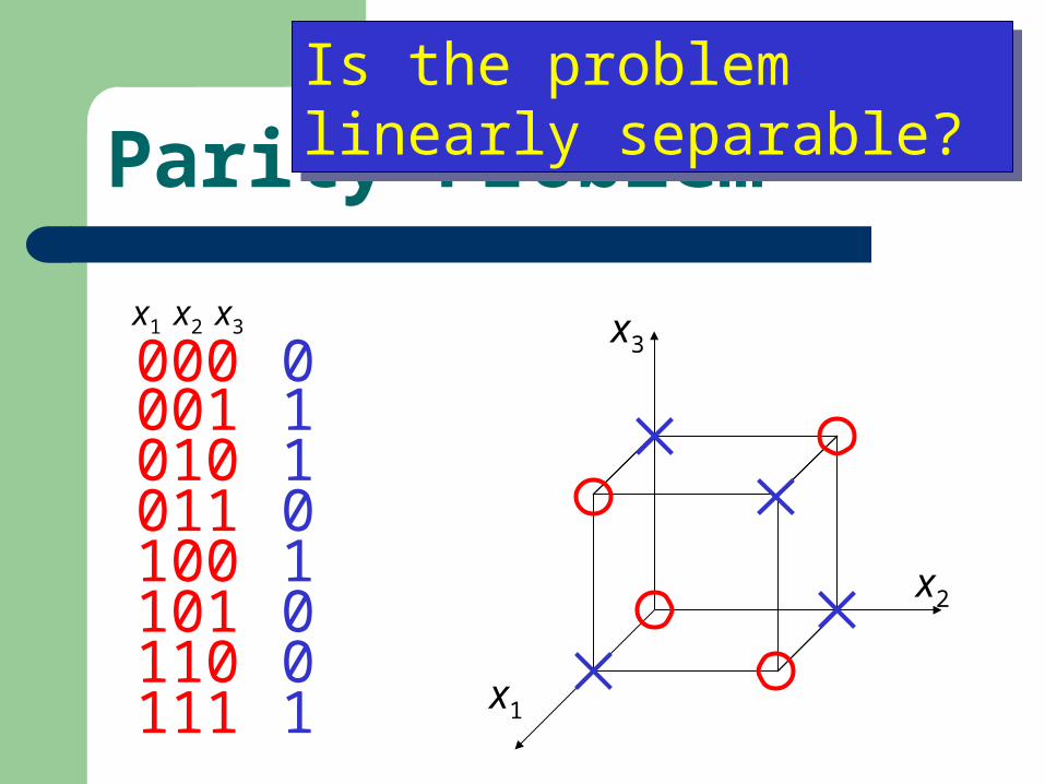
Parity Problem
x1
x2
x30110100
000001010011100101110111 1
x1 x2 x3
Is the problem linearly separable?Is the problem linearly separable?
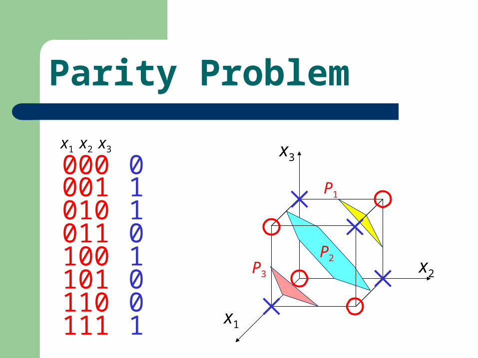
Parity Problem
x1
x2
x30110100
000001010011100101110111 1
x1 x2 x3
P1
P2P3
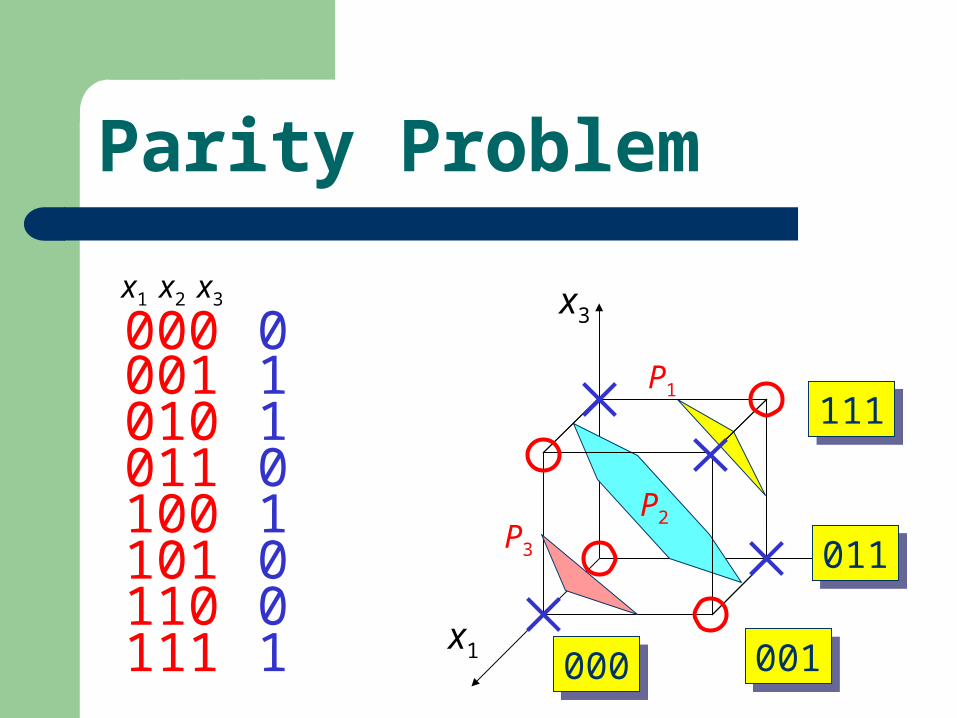
Parity Problem
0110100
000001010011100101110111 1
x1 x2 x3
x1
x2
x3
P1
P2P3
111111
011011
001001000000

Parity Problem
x1
x2
x3
P1
P2P3
111111
011011
001001000000
P1
x1 x2 x3
y1
P2
y2
P3
y3
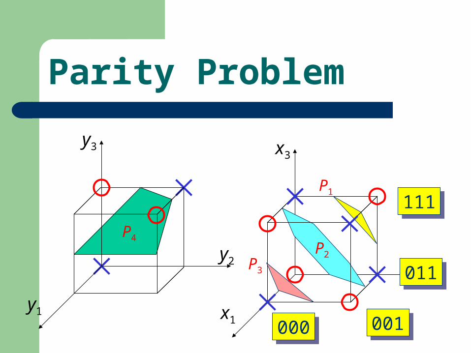
Parity Problem
x1
x2
x3
P1
P2P3
111111
011011
001001000000y1
y2
y3
P4
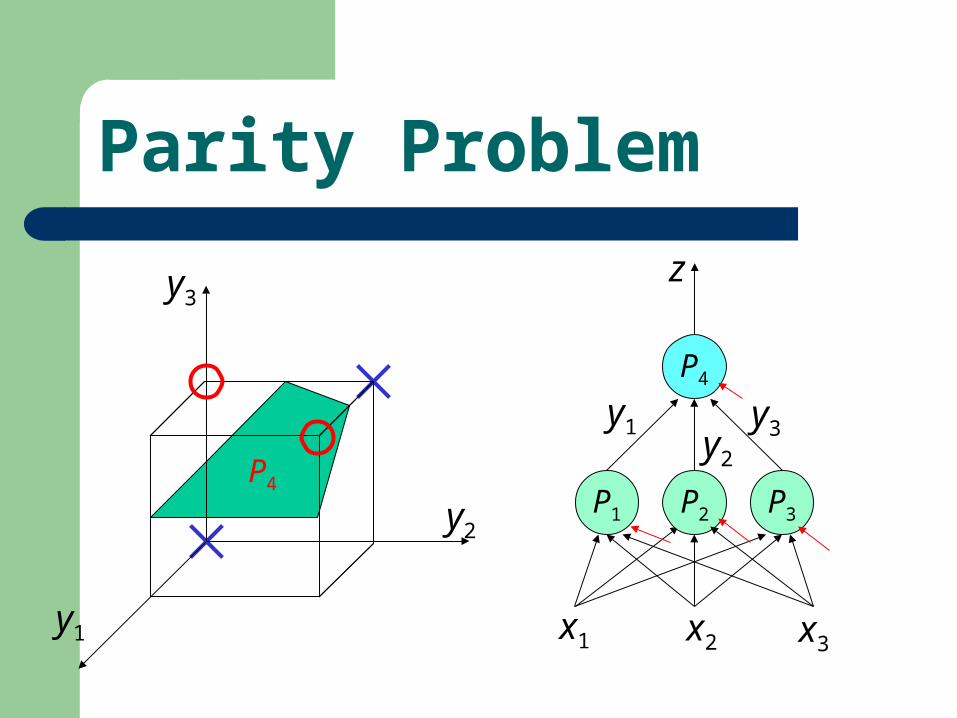
Parity Problem
y1
y2
y3
P4P1
x1 x2 x3
P2 P3
y1
z
y3
P4
y2
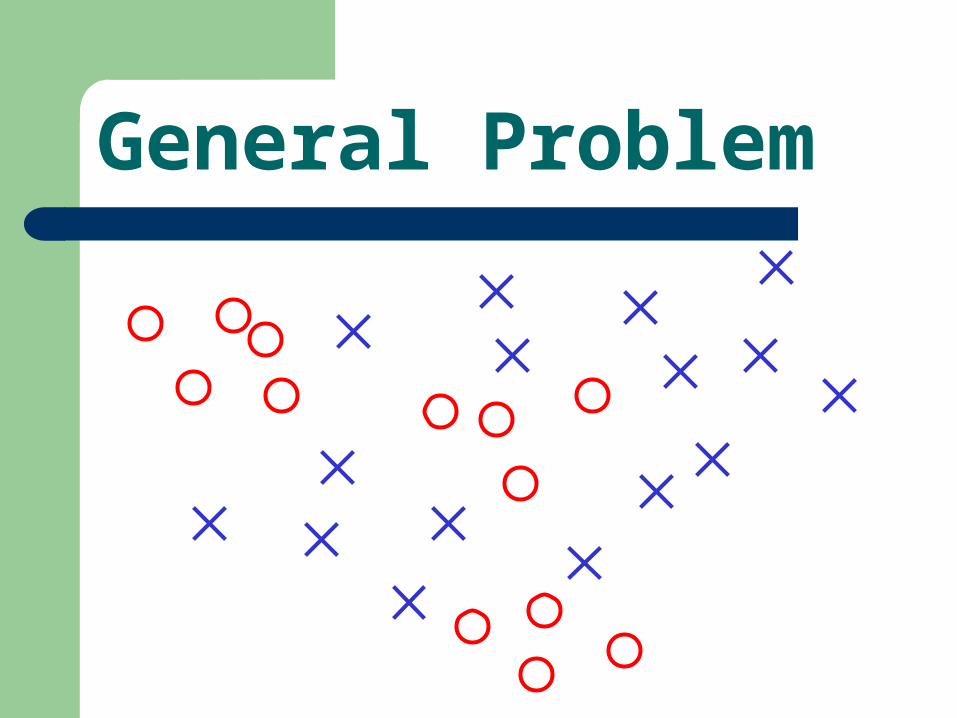
General Problem
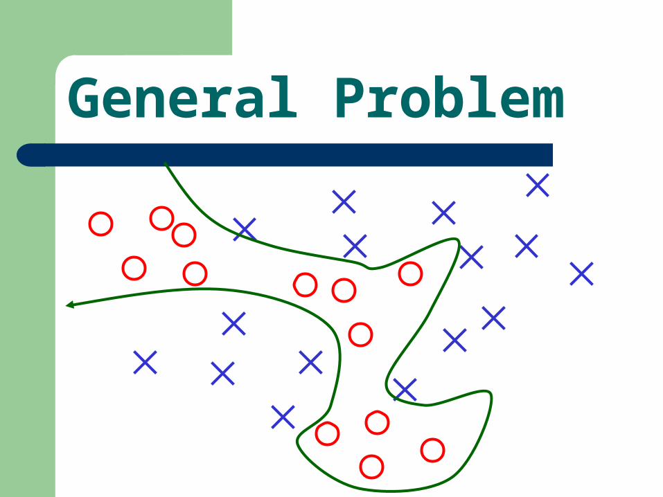
General Problem
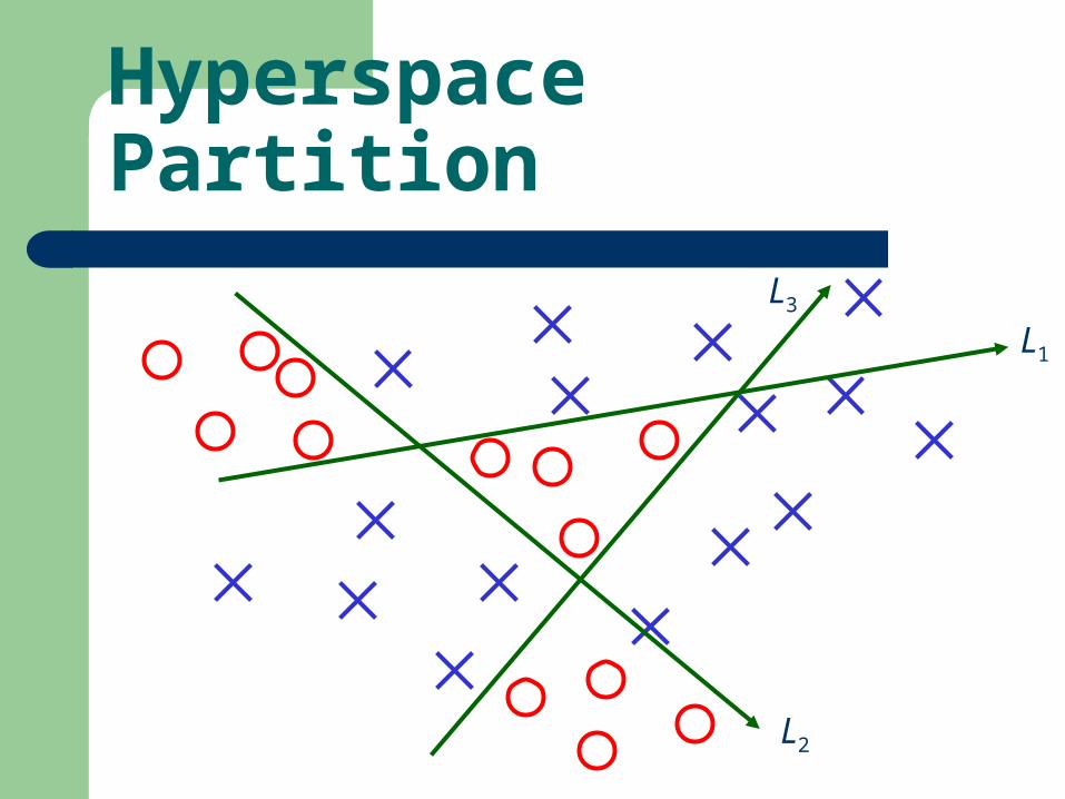
Hyperspace Partition
L1
L2
L3
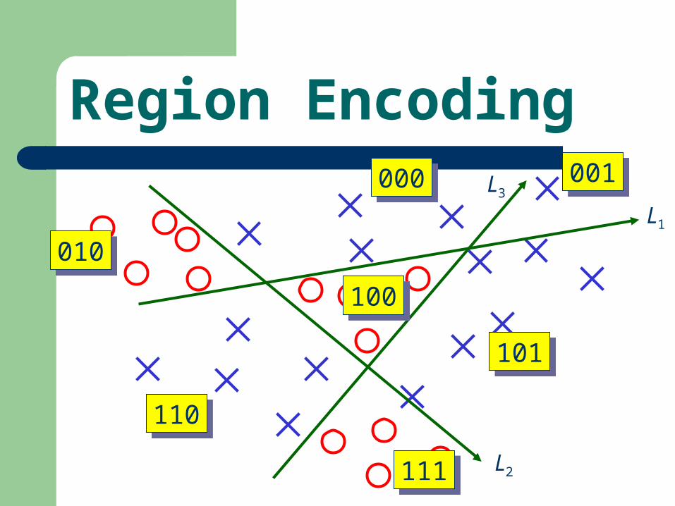
Region Encoding
101101
L1
L2
L3001001000000
010010
110110
111111
100100
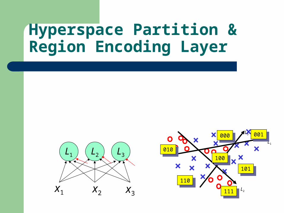
Hyperspace Partition & Region Encoding Layer
101101
L1
L2
L3001001
000000
010010
110110
111111
100100L1
x1 x2 x3
L2 L3
101
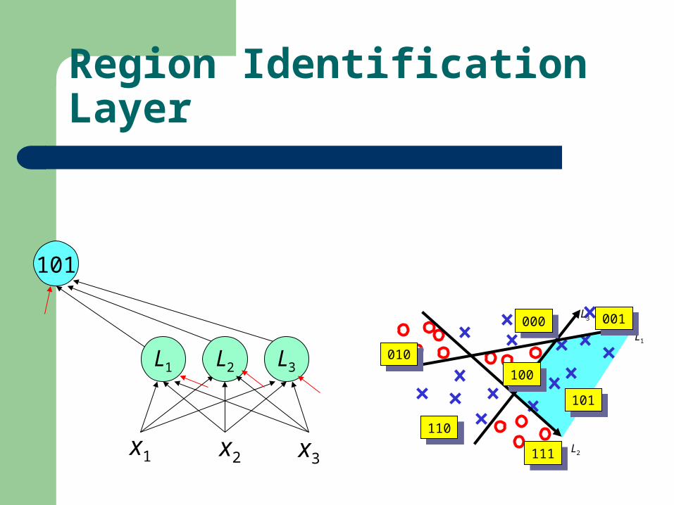
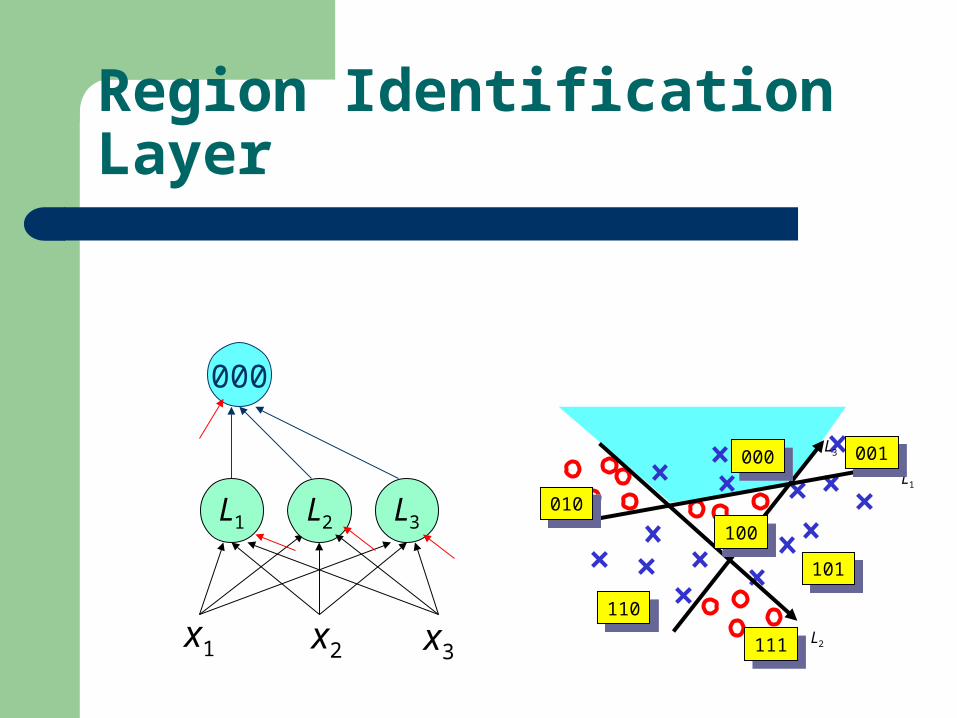
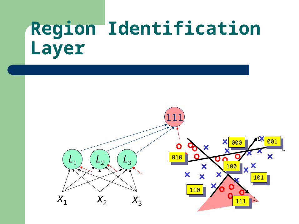
Region Identification Layer
101101
L1
L2
L3001001
000000
010010
110110
111111
100100L1
x1 x2 x3
L2 L3
001
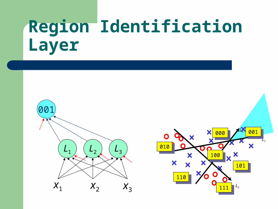
Region Identification Layer
101101
L1
L2
L3001001
000000
010010
110110
111111
100100L1
x1 x2 x3
L2 L3
000
Region Identification Layer
101101
L1
L2
L3001001
000000
010010
110110
111111
100100L1
x1 x2 x3
L2 L3
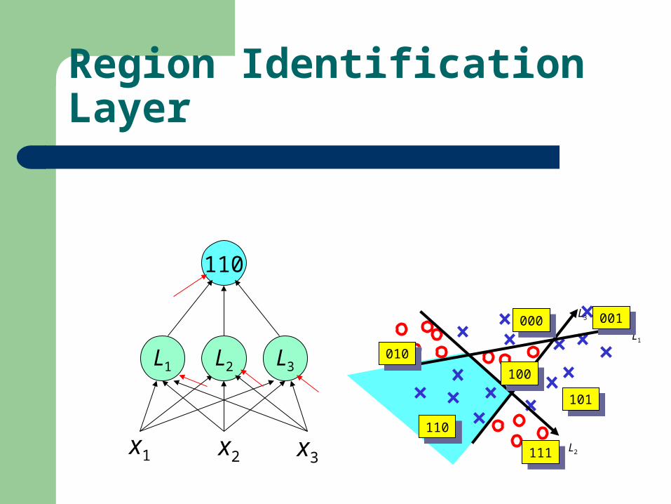
110
Region Identification Layer
101101
L1
L2
L3001001
000000
010010
110110
111111
100100L1
x1 x2 x3
L2 L3
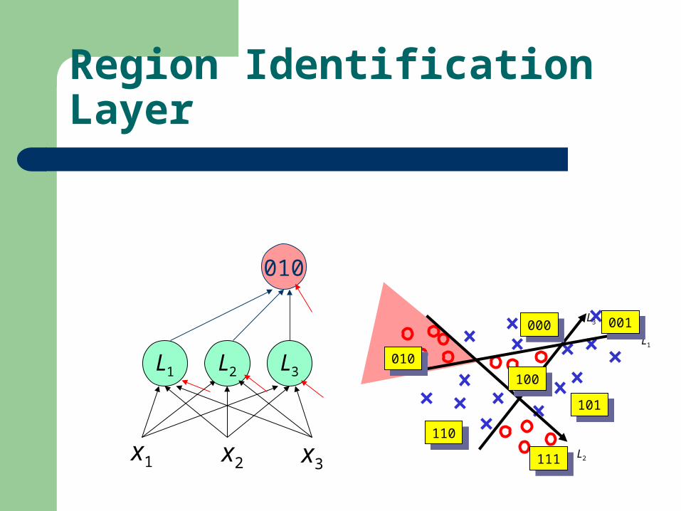
010
Region Identification Layer
101101
L1
L2
L3001001
000000
010010
110110
111111
100100L1
x1 x2 x3
L2 L3
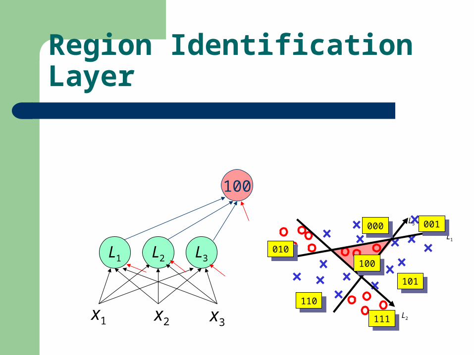
100
Region Identification Layer
101101
L1
L2
L3001001
000000
010010
110110
111111
100100L1
x1 x2 x3
L2 L3
111
Region Identification Layer
101101
L1
L2
L3001001
000000
010010
110110
111111
100100L1
x1 x2 x3
L2 L3
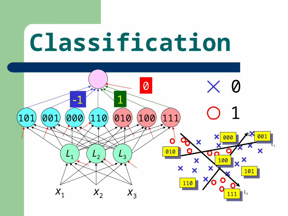
Classification
101101
L1
L2
L3001001
000000
010010
110110
111111
100100L1
x1 x2 x3
L2 L3
001101101 001 000 110 010 100 111
0
11 1
0

Feed-Forward Neural Networks
Back Propagation Learning algorithm
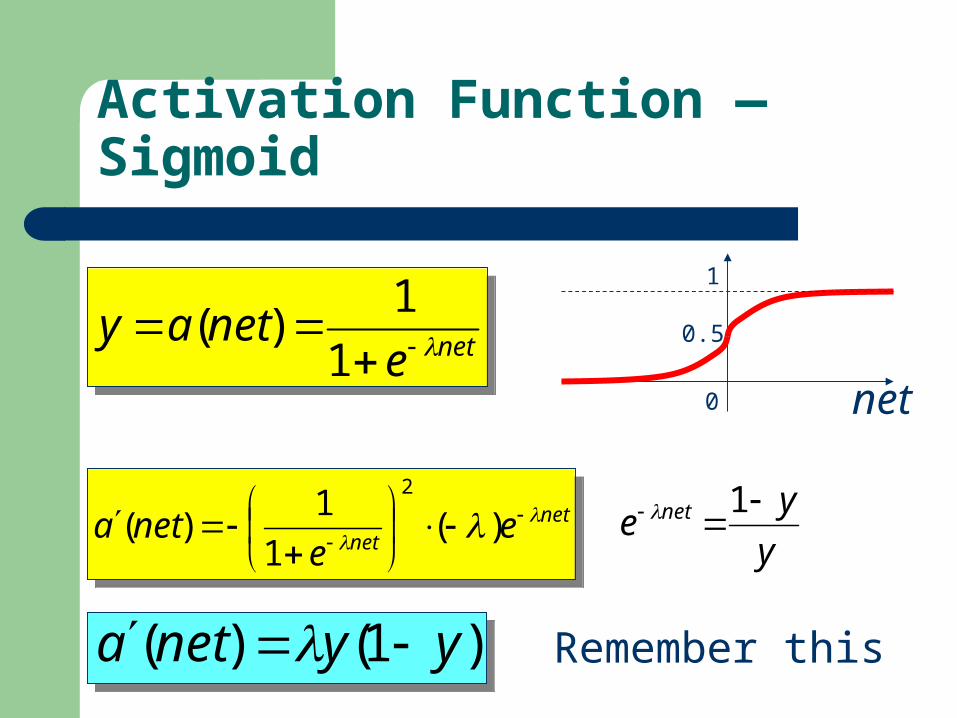
Activation Function — Sigmoid
netenetay
1
1)( nete
netay
1
1)(
netnet
ee
neta
)(1
1)(
2net
nete
eneta
)(1
1)(
2
y
ye net
1
)1()( yyneta )1()( yyneta
net
1
0.5
0
Remember this
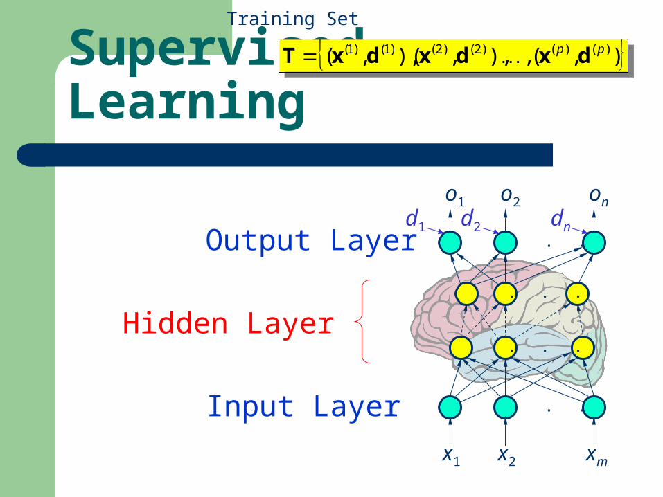
Supervised Learning
. . .
. . .
. . .
. . .
x1 x2 xm
o1 o2 on
Hidden Layer
Input Layer
Output Layer
),(,),,(),,( )()()2()2()1()1( pp dxdxdxT ),(,),,(),,( )()()2()2()1()1( pp dxdxdxT
Training Set
d1 d2 dn
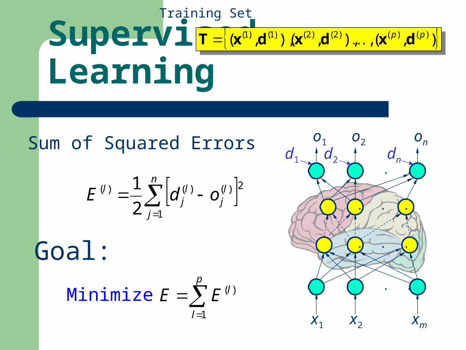
Supervised Learning
. . .
. . .
. . .
. . .
x1 x2 xm
o1 o2 on
d1 d2 dn
p
l
lEE1
)(
n
j
lj
lj
l odE1
2)()()(
2
1
Sum of Squared Errors
Goal:
Minimize
),(,),,(),,( )()()2()2()1()1( pp dxdxdxT ),(,),,(),,( )()()2()2()1()1( pp dxdxdxT
Training Set
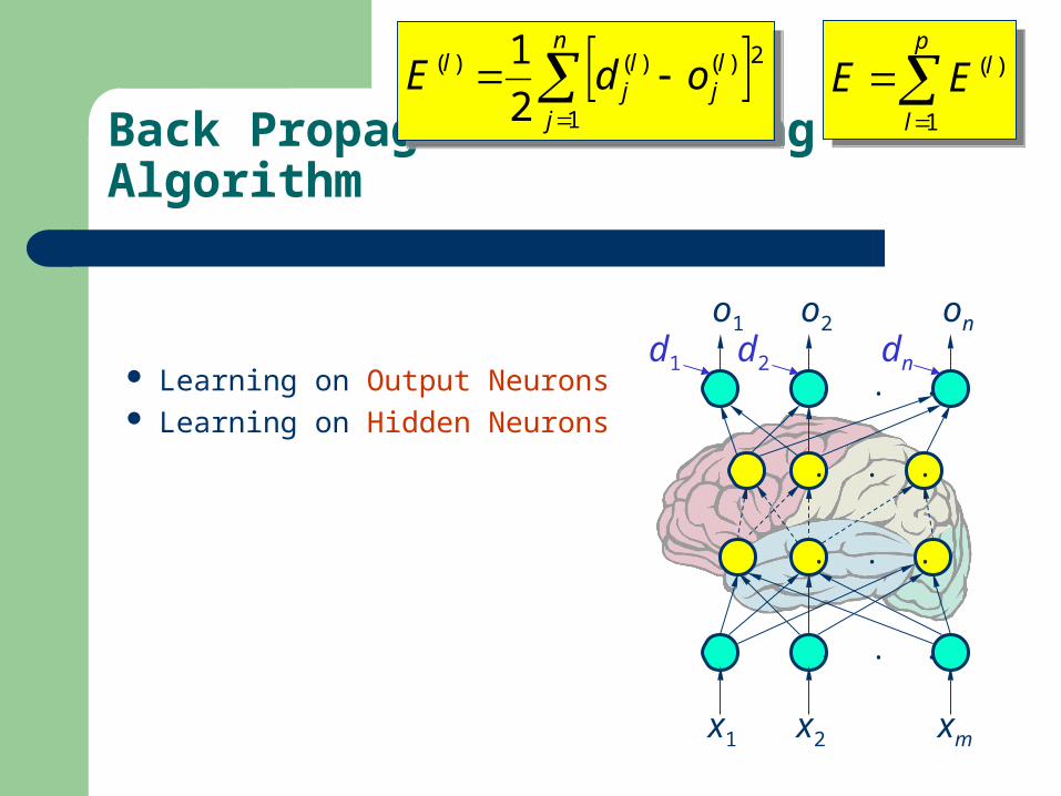
Back Propagation Learning Algorithm
. . .
. . .
. . .
. . .
x1 x2 xm
o1 o2 on
d1 d2 dn
p
l
lEE1
)(
p
l
lEE1
)(
n
j
lj
lj
l odE1
2)()()(
2
1
n
j
lj
lj
l odE1
2)()()(
2
1
Learning on Output Neurons Learning on Hidden Neurons
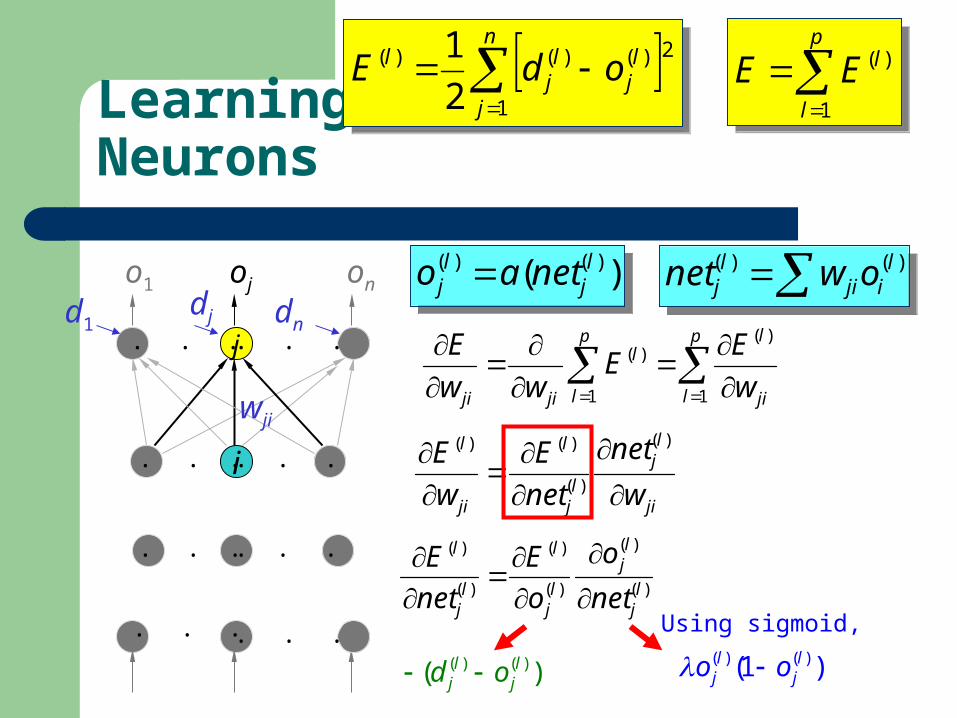
Learning on Output Neurons
. . .
j . . .
. . .
i . . .
o1 oj on
d1dj dn
. . .
. . .
. . .
. . .
wji
p
l ji
lp
l
l
jiji w
EE
ww
E
1
)(
1
)(
ji
lj
lj
l
ji
l
w
net
net
E
w
E
)(
)(
)()(
)( )()( lj
lj netao )( )()( l
jl
j netao )()( liji
lj ownet )()( l
ijil
j ownet
? ?
p
l
lEE1
)(
p
l
lEE1
)(
n
j
lj
lj
l odE1
2)()()(
2
1
n
j
lj
lj
l odE1
2)()()(
2
1
Learning on Output Neurons
. . .
j . . .
. . .
i . . .
o1 oj on
d1dj dn
. . .
. . .
. . .
. . .
wji
p
l
lEE1
)(
p
l
lEE1
)(
n
j
lj
lj
l odE1
2)()()(
2
1
n
j
lj
lj
l odE1
2)()()(
2
1
)(
)(
)(
)(
)(
)(
lj
lj
lj
l
lj
l
net
o
o
E
net
E
p
l ji
lp
l
l
jiji w
EE
ww
E
1
)(
1
)(
ji
lj
lj
l
ji
l
w
net
net
E
w
E
)(
)(
)()(
)( )()( lj
lj netao )( )()( l
jl
j netao )()( liji
lj ownet )()( l
ijil
j ownet
)( )()( lj
lj od
depends on the activation function
Learning on Output Neurons
. . .
j . . .
. . .
i . . .
o1 oj on
d1dj dn
. . .
. . .
. . .
. . .
wji
p
l
lEE1
)(
p
l
lEE1
)(
n
j
lj
lj
l odE1
2)()()(
2
1
n
j
lj
lj
l odE1
2)()()(
2
1
)(
)(
)(
)(
)(
)(
lj
lj
lj
l
lj
l
net
o
o
E
net
E
p
l ji
lp
l
l
jiji w
EE
ww
E
1
)(
1
)(
ji
lj
lj
l
ji
l
w
net
net
E
w
E
)(
)(
)()(
)( )()( lj
lj netao )( )()( l
jl
j netao )()( liji
lj ownet )()( l
ijil
j ownet
( ) ( )( )l lj jd o
( ) ( )(1 )l lj jo o
Using sigmoid,
Learning on Output Neurons
. . .
j . . .
. . .
i . . .
o1 oj on
d1dj dn
. . .
. . .
. . .
. . .
wji
p
l
lEE1
)(
p
l
lEE1
)(
n
j
lj
lj
l odE1
2)()()(
2
1
n
j
lj
lj
l odE1
2)()()(
2
1
)(
)(
)(
)(
)(
)(
lj
lj
lj
l
lj
l
net
o
o
E
net
E
p
l ji
lp
l
l
jiji w
EE
ww
E
1
)(
1
)(
ji
lj
lj
l
ji
l
w
net
net
E
w
E
)(
)(
)()(
)( )()( lj
lj netao )( )()( l
jl
j netao )()( liji
lj ownet )()( l
ijil
j ownet
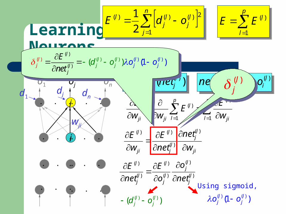
( ) ( )( )l lj jd o
( ) ( )(1 )l lj jo o
Using sigmoid,
( )lj
(( )
( )( ) ( ()
) ) )(
( ) (1 )ll
lj
lj j
l l lj jj
E
neto od o
Learning on Output Neurons
. . .
j . . .
. . .
i . . .
o1 oj on
d1dj dn
. . .
. . .
. . .
. . .
wji
p
l
lEE1
)(
p
l
lEE1
)(
n
j
lj
lj
l odE1
2)()()(
2
1
n
j
lj
lj
l odE1
2)()()(
2
1
p
l ji
lp
l
l
jiji w
EE
ww
E
1
)(
1
)(
ji
lj
lj
l
ji
l
w
net
net
E
w
E
)(
)(
)()(
)( )()( lj
lj netao )( )()( l
jl
j netao )()( liji
lj ownet )()( l
ijil
j ownet
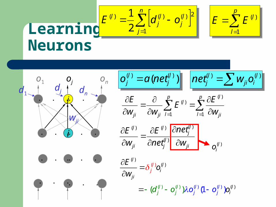
)(lio
( )( )( )
ll
iji
lj
Eo
w
( ( )) (( )( ) ) (1( )) l lj
l lj
lj ijd o o oo

Learning on Output Neurons
. . .
j . . .
. . .
i . . .
o1 oj on
d1dj dn
. . .
. . .
. . .
. . .
wji
p
l
lEE1
)(
p
l
lEE1
)(
n
j
lj
lj
l odE1
2)()()(
2
1
n
j
lj
lj
l odE1
2)()()(
2
1
p
l ji
lp
l
l
jiji w
EE
ww
E
1
)(
1
)(
ji
lj
lj
l
ji
l
w
net
net
E
w
E
)(
)(
)()(
)( )()( lj
lj netao )( )()( l
jl
j netao )()( liji
lj ownet )()( l
ijil
j ownet
)(lio
( )( )( )
ll
iji
lj
Eo
w
( ( )) (( )( ) ) (1( )) l lj
l lj
lj ijd o o oo
( ) ( )
1
pl
il
lj
ji
Eo
w
( ) ( )
1
pl
il
lj
ji
Eo
w
)(
1
)( li
p
l
ljji ow
)(
1
)( li
p
l
ljji ow
How to train the weights connecting to output neurons?
How to train the weights connecting to output neurons?
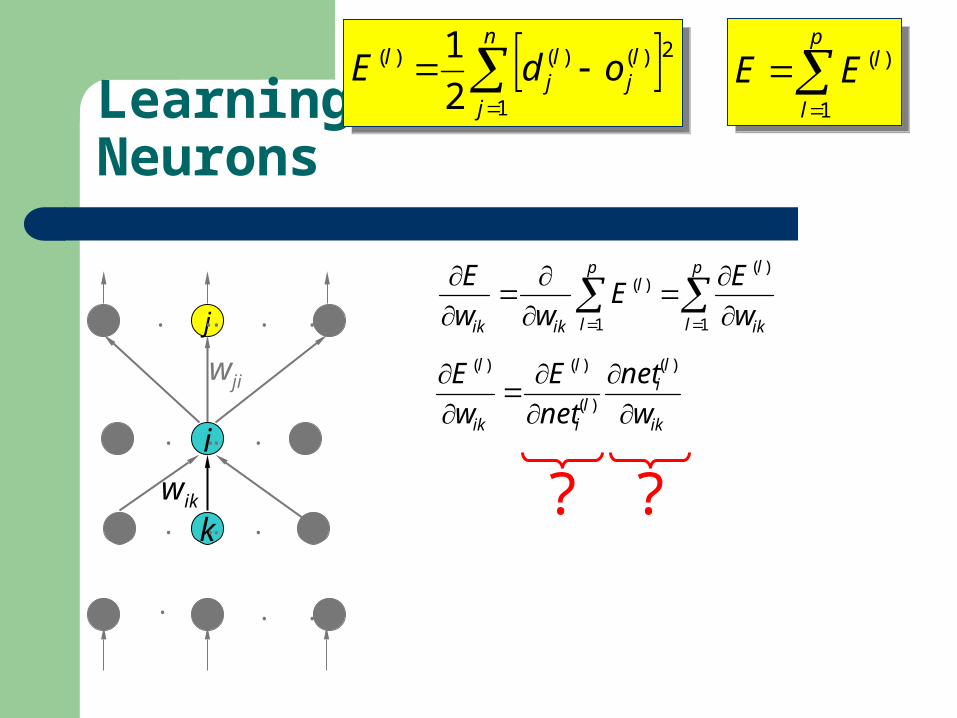
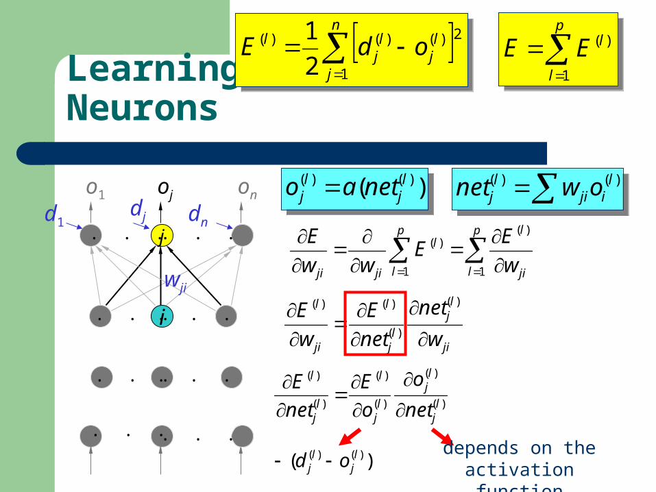
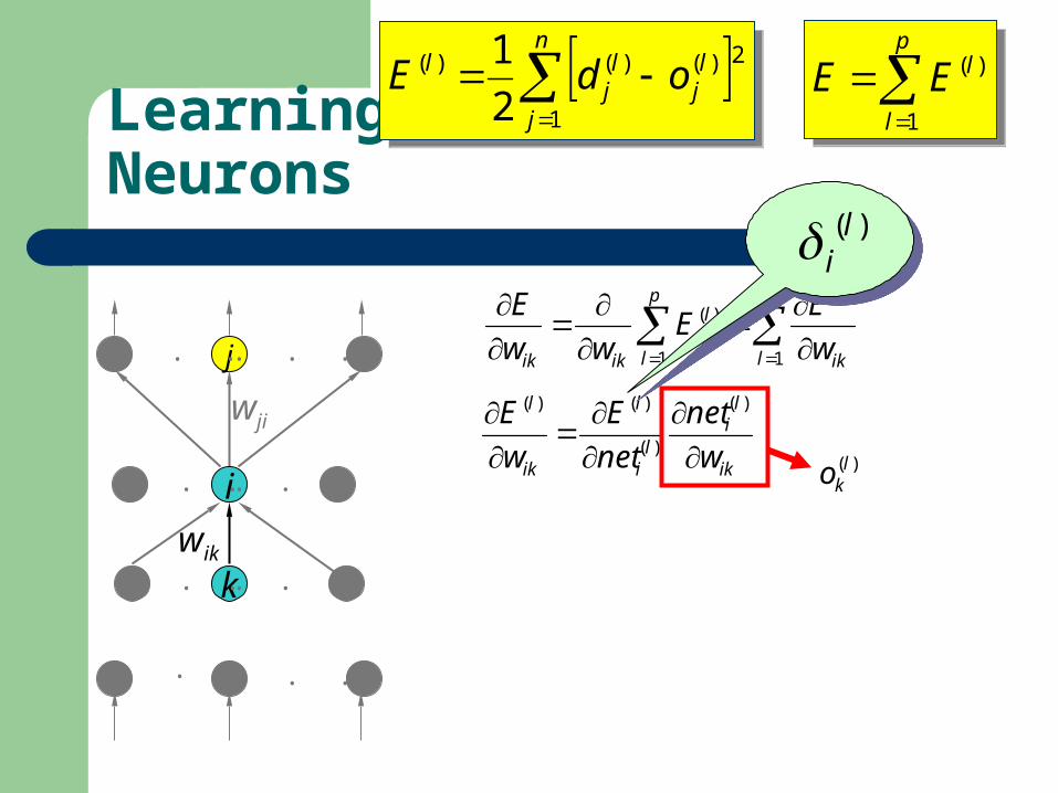
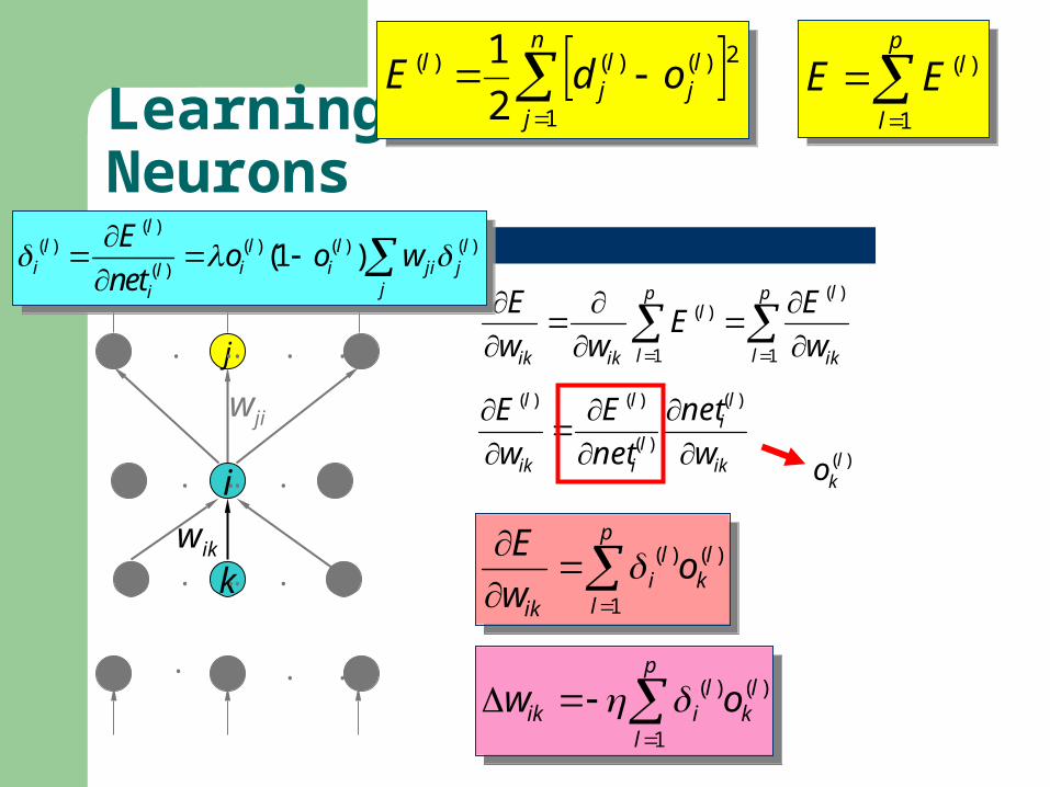
Learning on Hidden Neurons
p
l
lEE1
)(
p
l
lEE1
)(
n
j
lj
lj
l odE1
2)()()(
2
1
n
j
lj
lj
l odE1
2)()()(
2
1
. . .
j . . .
k . . .
i . . .
. . .
. . .
. . .
. . .
wik
wji
p
l ik
lp
l
l
ikik w
EE
ww
E
1
)(
1
)(
ik
li
li
l
ik
l
w
net
net
E
w
E
)(
)(
)()(
? ?
Learning on Hidden Neurons
p
l
lEE1
)(
p
l
lEE1
)(
n
j
lj
lj
l odE1
2)()()(
2
1
n
j
lj
lj
l odE1
2)()()(
2
1
. . .
j . . .
k . . .
i . . .
. . .
. . .
. . .
. . .
wik
wji
p
l ik
lp
l
l
ikik w
EE
ww
E
1
)(
1
)(
ik
li
li
l
ik
l
w
net
net
E
w
E
)(
)(
)()(
)(li
)(lko
Learning on Hidden Neurons
p
l
lEE1
)(
p
l
lEE1
)(
n
j
lj
lj
l odE1
2)()()(
2
1
n
j
lj
lj
l odE1
2)()()(
2
1
. . .
j . . .
k . . .
i . . .
. . .
. . .
. . .
. . .
wik
wji
p
l ik
lp
l
l
ikik w
EE
ww
E
1
)(
1
)(
ik
li
li
l
ik
l
w
net
net
E
w
E
)(
)(
)()(
)(li
)(lko
)(
)(
)(
)(
)(
)(
li
li
li
l
li
l
net
o
o
E
net
E
( ) ( )(1 )l li io o
( ) ( )(1 )l li io o ?

Learning on Hidden Neurons
p
l
lEE1
)(
p
l
lEE1
)(
n
j
lj
lj
l odE1
2)()()(
2
1
n
j
lj
lj
l odE1
2)()()(
2
1
. . .
j . . .
k . . .
i . . .
. . .
. . .
. . .
. . .
wik
wji
p
l ik
lp
l
l
ikik w
EE
ww
E
1
)(
1
)(
ik
li
li
l
ik
l
w
net
net
E
w
E
)(
)(
)()(
)(li
)(lko
)(
)(
)(
)(
)(
)(
li
li
li
l
li
l
net
o
o
E
net
E
jl
i
lj
lj
l
li
l
o
net
net
E
o
E)(
)(
)(
)(
)(
)(
)(lj jiw
( )( ) ( ) ( ) ( )
( )(1 )
ll l l l
i i i ji jlji
Eo o w
net
( )( ) ( ) ( ) ( )
( )(1 )
ll l l l
i i i ji jlji
Eo o w
net
( ) ( )(1 )l li io o
( ) ( )(1 )l li io o
Learning on Hidden Neurons
p
l
lEE1
)(
p
l
lEE1
)(
n
j
lj
lj
l odE1
2)()()(
2
1
n
j
lj
lj
l odE1
2)()()(
2
1
. . .
j . . .
k . . .
i . . .
. . .
. . .
. . .
. . .
wik
wji
p
l ik
lp
l
l
ikik w
EE
ww
E
1
)(
1
)(
ik
li
li
l
ik
l
w
net
net
E
w
E
)(
)(
)()(
)(lko
)(
1
)( lk
p
l
li
ik
ow
E
)(
1
)( lk
p
l
li
ik
ow
E
)(
1
)( lk
p
l
liik ow
)(
1
)( lk
p
l
liik ow
( )( ) ( ) ( ) ( )
( )(1 )
ll l l l
i i i ji jlji
Eo o w
net
( )( ) ( ) ( ) ( )
( )(1 )
ll l l l
i i i ji jlji
Eo o w
net

Back Propagationo1 oj on
. . .
j . . .
k . . .
i . . .
d1dj dn
. . .
. . .
. . .
. . .
x1 xm. . .
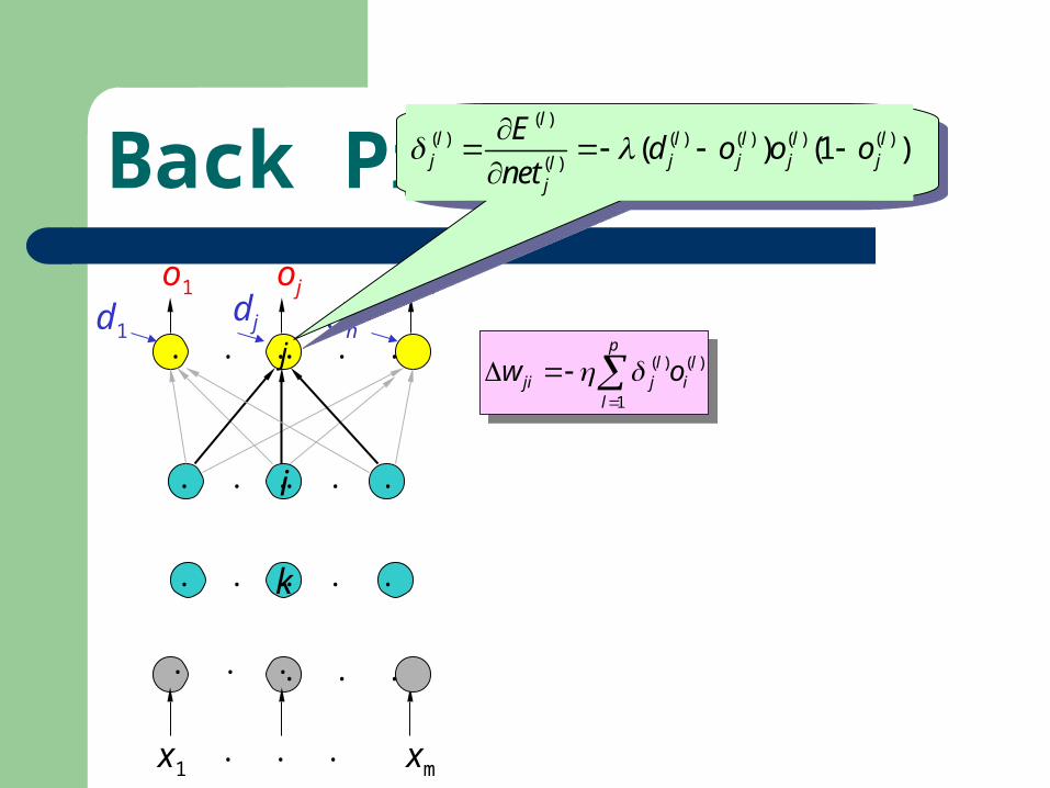
Back Propagationo1 oj on
. . .
j . . .
k . . .
i . . .
d1dj dn
. . .
. . .
. . .
. . .
x1 xm. . .
( )( ) ( ) ( ) ( ) ( )
( )( ) (1 )
ll l l l l
j j j j jlj
Ed o o o
net
)(
1
)( li
p
l
ljji ow
)(
1
)( li
p
l
ljji ow
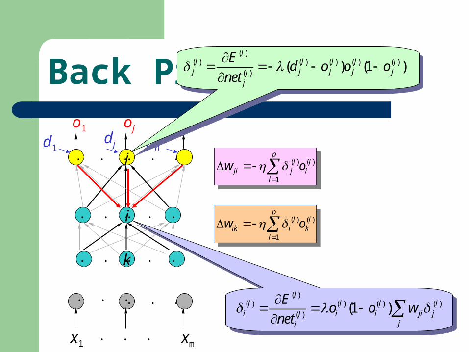
Back Propagationo1 oj on
. . .
j . . .
k . . .
i . . .
d1dj dn
. . .
. . .
. . .
. . .
x1 xm. . .
( )( ) ( ) ( ) ( ) ( )
( )( ) (1 )
ll l l l l
j j j j jlj
Ed o o o
net
)(
1
)( li
p
l
ljji ow
)(
1
)( li
p
l
ljji ow
( )( ) ( ) ( ) ( )
( )(1 )
ll l l l
i i i ji jlji
Eo o w
net
)(
1
)( lk
p
l
liik ow
)(
1
)( lk
p
l
liik ow
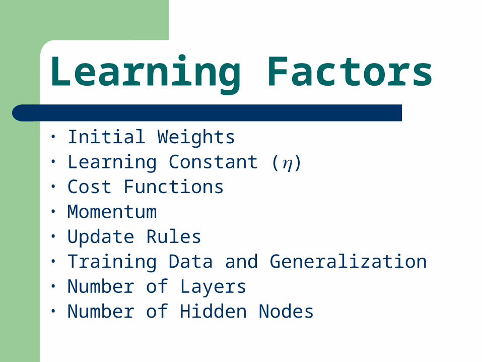
Learning Factors• Initial Weights• Learning Constant ()• Cost Functions• Momentum• Update Rules• Training Data and Generalization• Number of Layers• Number of Hidden Nodes

Reading Assignments Shi Zhong and Vladimir Cherkassky, “Factors Controlling Generalization Ability of M
LP Networks.” In Proc. IEEE Int. Joint Conf. on Neural Networks, vol. 1, pp. 625-630, Washington DC. July 1999. (http://www.cse.fau.edu/~zhong/pubs.htm)
Rumelhart, D. E., Hinton, G. E., and Williams, R. J. (1986b). "Learning Internal Representations by Error Propagation," in Parallel Distributed Processing: Explorations in the Microstructure of Cognition, vol. I, D. E. Rumelhart, J. L. McClelland, and the PDP Research Group. MIT Press, Cambridge (1986).
(http://www.cnbc.cmu.edu/~plaut/85-419/papers/RumelhartETAL86.backprop.pdf).