Embed Size (px)
Citation preview
Outline Linearly Nonseparable Pattern Error Back Propagation Algorithm Universal Approximator Learning Factors Adaptive MLP
Neural NetworksLecture 3:Multi-Layer Perceptron
H.A TalebiFarzaneh Abdollahi
Department of Electrical Engineering
Amirkabir University of Technology
Winter 2011H. A. Talebi, Farzaneh Abdollahi Neural Networks Lecture 3 1/52
Outline Linearly Nonseparable Pattern Error Back Propagation Algorithm Universal Approximator Learning Factors Adaptive MLP
Linearly Nonseparable Pattern Classification
Error Back Propagation AlgorithmFeedforward Recall and Error Back-Propagation
Multilayer Neural Nets as Universal Approximators
Learning FactorsInitial WeightsErrorTraining versus GeneralizationNecessary Number of Patterns for Training setNecessary Number of Hidden NeuronsLearning ConstantSteepness of Activation FunctionBatch versus Incremental UpdatesNormalizationOffline versus Online TrainingLevenberg-Marquardt Training
Adaptive MLPH. A. Talebi, Farzaneh Abdollahi Neural Networks Lecture 3 2/52
Outline Linearly Nonseparable Pattern Error Back Propagation Algorithm Universal Approximator Learning Factors Adaptive MLP
Linearly Nonseparable Pattern Classification
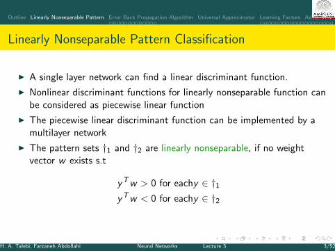
I A single layer network can find a linear discriminant function.
I Nonlinear discriminant functions for linearly nonseparable function canbe considered as piecewise linear function
I The piecewise linear discriminant function can be implemented by amultilayer network
I The pattern sets †1 and †2 are linearly nonseparable, if no weightvector w exists s.t
yTw > 0 for eachy ∈ †1yTw < 0 for eachy ∈ †2
H. A. Talebi, Farzaneh Abdollahi Neural Networks Lecture 3 3/52
Outline Linearly Nonseparable Pattern Error Back Propagation Algorithm Universal Approximator Learning Factors Adaptive MLP
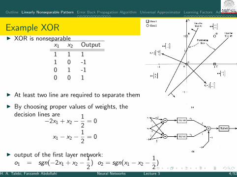
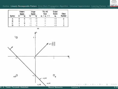
Example XORI XOR is nonseparable
x1 x2 Output
1 1 11 0 -10 1 -10 0 1
I At least two line are required to separate them
I By choosing proper values of weights, thedecision lines are
−2x1 + x2 −1
2= 0
x1 − x2 −1
2= 0
I output of the first layer network:o1 = sgn(−2x1 + x2 −
1
2) o2 = sgn(x1 − x2 −
1
2)
H. A. Talebi, Farzaneh Abdollahi Neural Networks Lecture 3 4/52
Outline Linearly Nonseparable Pattern Error Back Propagation Algorithm Universal Approximator Learning Factors Adaptive MLP
H. A. Talebi, Farzaneh Abdollahi Neural Networks Lecture 3 5/52
Outline Linearly Nonseparable Pattern Error Back Propagation Algorithm Universal Approximator Learning Factors Adaptive MLP
I The main idea of solving linearly nonseparable patterns is:I The set of linearly nonseparable pattern is mapped into the image space
where it becomes linearly separable.I This can be done by proper selecting weights of the first layer(s)I Then in the next layer they can be easily classified
I Increasing # of neurons in the middle layer increases # of lines.I ∴ provides nonlinear and more complicated discriminant functions
I The pattern parameters and center of clusters are not always known apriori
I ∴ A stepwise supervised learning algorithm is required to calculate theweights
H. A. Talebi, Farzaneh Abdollahi Neural Networks Lecture 3 6/52
Outline Linearly Nonseparable Pattern Error Back Propagation Algorithm Universal Approximator Learning Factors Adaptive MLP
Delta Learning Rule for Feedforward Multilayer Perceptron
I The training algorithm is called error back propagation (EBP) trainingalgorithm
I If a submitted pattern provides an output far from desired value, theweights and thresholds are adjusted s.t. the current mean squareclassification error is reduced.
I The training is continued/repeated for all patterns until the trainingset provide an acceptable overall error.
I Usually the mapping error is computed over the full training set.I EBP alg. is working in two stages:
1. The trained network operates feedforward to obtain output of thenetwork
2. The weight adjustment propagate backward from output layer throughhidden layer toward input layer.
H. A. Talebi, Farzaneh Abdollahi Neural Networks Lecture 3 7/52
Outline Linearly Nonseparable Pattern Error Back Propagation Algorithm Universal Approximator Learning Factors Adaptive MLP
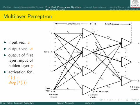
Multilayer Perceptron
I input vec. z
I output vec. o
I output of firstlayer, input ofhidden layer y
I activation fcn.Γ(.) =diag{f (.)}
H. A. Talebi, Farzaneh Abdollahi Neural Networks Lecture 3 8/52
Outline Linearly Nonseparable Pattern Error Back Propagation Algorithm Universal Approximator Learning Factors Adaptive MLP
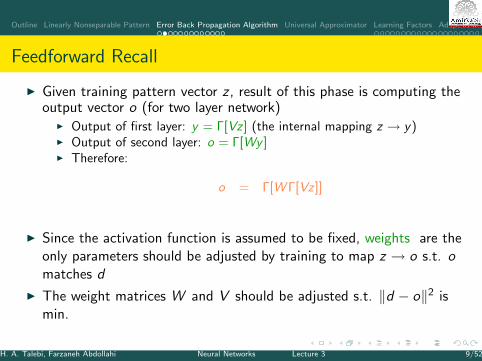
Feedforward Recall
I Given training pattern vector z , result of this phase is computing theoutput vector o (for two layer network)
I Output of first layer: y = Γ[Vz ] (the internal mapping z → y)I Output of second layer: o = Γ[Wy ]I Therefore:
o = Γ[W Γ[Vz ]]
I Since the activation function is assumed to be fixed, weights are theonly parameters should be adjusted by training to map z → o s.t. omatches d
I The weight matrices W and V should be adjusted s.t. ‖d − o‖2 ismin.
H. A. Talebi, Farzaneh Abdollahi Neural Networks Lecture 3 9/52
Outline Linearly Nonseparable Pattern Error Back Propagation Algorithm Universal Approximator Learning Factors Adaptive MLP
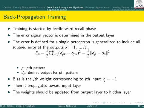
Back-Propagation Training
I Training is started by feedforward recall phase
I The error signal vector is determined in the output layer
I The error is defined for a single perceptron is generalized to include allsquared error at the outputs k = 1, ...,K
Ep =1
2ΣK
k=1(dpk − opk)2 =1
2‖dp − op‖2
I p: pth patternI dp: desired output for pth pattern
I Bias is the jth weight corresponding to jth input yj = −1
I Then it propagates toward input layer
I The weights should be updated from output layer to hidden layer
H. A. Talebi, Farzaneh Abdollahi Neural Networks Lecture 3 10/52
Outline Linearly Nonseparable Pattern Error Back Propagation Algorithm Universal Approximator Learning Factors Adaptive MLP
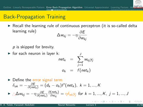
Back-Propagation Training
I Recall the learning rule of continuous perceptron (it is so-called deltalearning rule)
∆wkj = −η ∂E
∂wkj
p is skipped for brevity.
I for each neuron in layer k:
netk =J∑
j=1
wkjyj
ok = f (netk)
I Define the error signal termδok = − ∂E
∂(netk ) = (dk − ok)f ′(netk), k = 1, ...,K
I ∴∆wkj = −η ∂E∂(netk )
∂(netk )∂wkj
= ηδokyj for k = 1, ...,K , j = 1, ..., J
H. A. Talebi, Farzaneh Abdollahi Neural Networks Lecture 3 11/52
Outline Linearly Nonseparable Pattern Error Back Propagation Algorithm Universal Approximator Learning Factors Adaptive MLP
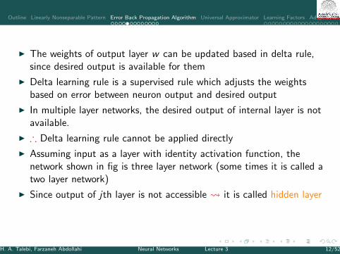
I The weights of output layer w can be updated based in delta rule,since desired output is available for them
I Delta learning rule is a supervised rule which adjusts the weightsbased on error between neuron output and desired output
I In multiple layer networks, the desired output of internal layer is notavailable.
I ∴ Delta learning rule cannot be applied directly
I Assuming input as a layer with identity activation function, thenetwork shown in fig is three layer network (some times it is called atwo layer network)
I Since output of jth layer is not accessible it is called hidden layer
H. A. Talebi, Farzaneh Abdollahi Neural Networks Lecture 3 12/52
Outline Linearly Nonseparable Pattern Error Back Propagation Algorithm Universal Approximator Learning Factors Adaptive MLP
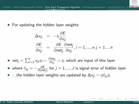
I For updating the hidden layer weights:
∆vji = −η ∂E
∂vji
∂E
∂vji=
∂E
∂netj
∂netj∂vji
, i = 1, ..., n j = 1, ...n
I netj =∑I
i=1 vjizi ∂netj∂vji
= zi which are input of this layer
I where δyj = − ∂E∂(netj )
for j = 1, ..., J is signal error of hidden layer
I ∴ the hidden layer weights are updated by ∆vji = ηδyjzi
H. A. Talebi, Farzaneh Abdollahi Neural Networks Lecture 3 13/52
Outline Linearly Nonseparable Pattern Error Back Propagation Algorithm Universal Approximator Learning Factors Adaptive MLP
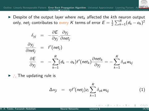
I Despite of the output layer where netk affected the kth neuron outputonly, netj contributes to every K terms of error E = 1
2
∑Rk=1(dk − ok)2
δyj = −∂E
∂yj.∂yj
∂netj∂yj
∂netj= f ′(netj)
∂E
∂yj= −
R∑k=1
(dk − ok)f ′(netk)∂netk∂yj
= −R∑
k=1
δokwkj
I ∴ The updating rule is
∆vji = ηf ′(netj)zi
R∑k=1
δokwkj (1)
H. A. Talebi, Farzaneh Abdollahi Neural Networks Lecture 3 14/52
Outline Linearly Nonseparable Pattern Error Back Propagation Algorithm Universal Approximator Learning Factors Adaptive MLP
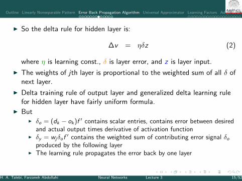
I So the delta rule for hidden layer is:
∆v = ηδz (2)
where η is learning const., δ is layer error, and z is layer input.
I The weights of jth layer is proportional to the weighted sum of all δ ofnext layer.
I Delta training rule of output layer and generalized delta learning rulefor hidden layer have fairly uniform formula.
I ButI δo = (dk − ok)f ′ contains scalar entries, contains error between desired
and actual output times derivative of activation functionI δy = wjδo f
′ contains the weighted sum of contributing error signal δoproduced by the following layer
I The learning rule propagates the error back by one layer
H. A. Talebi, Farzaneh Abdollahi Neural Networks Lecture 3 15/52

Outline Linearly Nonseparable Pattern Error Back Propagation Algorithm Universal Approximator Learning Factors Adaptive MLP
Back-Propagation Training
I Assuming sigmoid activation function, its time derivative is
f ′(net) =
{o(1− o) unipolar : f (net) = 1
1+exp(−λnet) , λ = 112(1− o2) bipolar : f (net) = 2
1+exp(−λnet) − 1, λ = 1
H. A. Talebi, Farzaneh Abdollahi Neural Networks Lecture 3 16/52
Outline Linearly Nonseparable Pattern Error Back Propagation Algorithm Universal Approximator Learning Factors Adaptive MLP
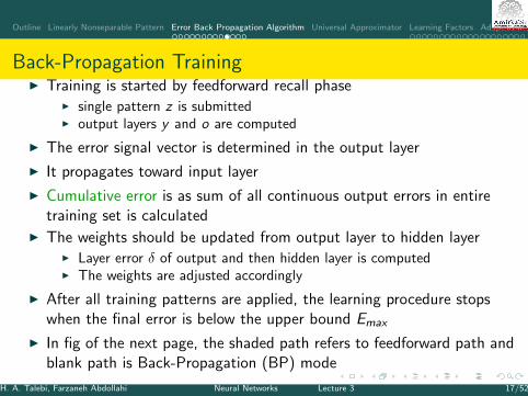
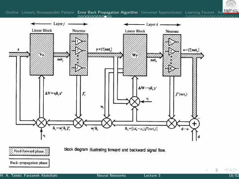
Back-Propagation TrainingI Training is started by feedforward recall phase
I single pattern z is submittedI output layers y and o are computed
I The error signal vector is determined in the output layer
I It propagates toward input layer
I Cumulative error is as sum of all continuous output errors in entiretraining set is calculated
I The weights should be updated from output layer to hidden layerI Layer error δ of output and then hidden layer is computedI The weights are adjusted accordingly
I After all training patterns are applied, the learning procedure stopswhen the final error is below the upper bound Emax
I In fig of the next page, the shaded path refers to feedforward path andblank path is Back-Propagation (BP) mode
H. A. Talebi, Farzaneh Abdollahi Neural Networks Lecture 3 17/52
Outline Linearly Nonseparable Pattern Error Back Propagation Algorithm Universal Approximator Learning Factors Adaptive MLP
H. A. Talebi, Farzaneh Abdollahi Neural Networks Lecture 3 18/52
Outline Linearly Nonseparable Pattern Error Back Propagation Algorithm Universal Approximator Learning Factors Adaptive MLP
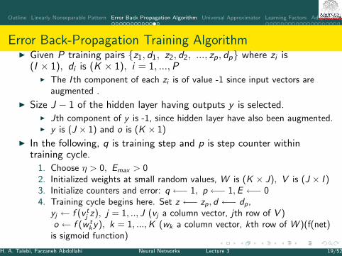
Error Back-Propagation Training AlgorithmI Given P training pairs {z1, d1, z2, d2, ..., zp, dp} where zi is
(I × 1), di is (K × 1), i = 1, ...,PI The I th component of each zi is of value -1 since input vectors are
augmented .
I Size J − 1 of the hidden layer having outputs y is selected.I Jth component of y is -1, since hidden layer have also been augmented.I y is (J × 1) and o is (K × 1)
I In the following, q is training step and p is step counter withintraining cycle.
1. Choose η > 0, Emax > 02. Initialized weights at small random values, W is (K × J), V is (J × I )3. Initialize counters and error: q ←− 1, p ←− 1,E ←− 04. Training cycle begins here. Set z ←− zp, d ←− dp,
yj ← f (v tj z), j = 1, .., J (vj a column vector, jth row of V )
o ← f (w tky), k = 1, ...,K (wk a column vector, kth row of W )(f(net)
is sigmoid function)
H. A. Talebi, Farzaneh Abdollahi Neural Networks Lecture 3 19/52
Outline Linearly Nonseparable Pattern Error Back Propagation Algorithm Universal Approximator Learning Factors Adaptive MLP
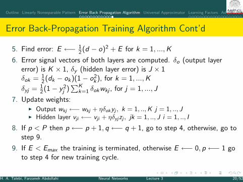
Error Back-Propagation Training Algorithm Cont’d
5. Find error: E ←− 12(d − o)2 + E for k = 1, ...,K
6. Error signal vectors of both layers are computed. δo (output layererror) is K × 1, δy (hidden layer error) is J × 1δok = 1
2(dk − ok)(1− o2k ), for k = 1, ...,K
δyj = 12(1− y2
j )∑K
k=1 δokwkj , for j = 1, ..., J
7. Update weights:I Output wkj ←− wkj + ηδokyj , k = 1, ..,K j = 1, .., JI Hidden layer vji ←− vji + ηδyjzj , jk = 1, .., J i = 1, .., I
8. If p < P then p ←− p + 1, q ←− q + 1, go to step 4, otherwise, go tostep 9.
9. If E < Emax the training is terminated, otherwise E ←− 0, p ←− 1 goto step 4 for new training cycle.
H. A. Talebi, Farzaneh Abdollahi Neural Networks Lecture 3 20/52
Outline Linearly Nonseparable Pattern Error Back Propagation Algorithm Universal Approximator Learning Factors Adaptive MLP
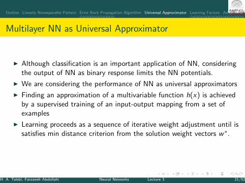
Multilayer NN as Universal Approximator
I Although classification is an important application of NN, consideringthe output of NN as binary response limits the NN potentials.
I We are considering the performance of NN as universal approximators
I Finding an approximation of a multivariable function h(x) is achievedby a supervised training of an input-output mapping from a set ofexamples
I Learning proceeds as a sequence of iterative weight adjustment until issatisfies min distance criterion from the solution weight vectors w∗.
H. A. Talebi, Farzaneh Abdollahi Neural Networks Lecture 3 21/52
Outline Linearly Nonseparable Pattern Error Back Propagation Algorithm Universal Approximator Learning Factors Adaptive MLP
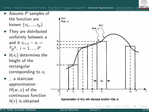
I Assume P samples ofthe function areknown {x1, ..., xp}
I They are distributeduniformly between aand b xi+1 − xi =b−aP , i = 1, ...,P
I h(xi ) determines theheight of therectangularcorresponding to xi
I ∴ a staircaseapproximationH(w , x) of thecontinuous functionh(x) is obtained
H. A. Talebi, Farzaneh Abdollahi Neural Networks Lecture 3 22/52
Outline Linearly Nonseparable Pattern Error Back Propagation Algorithm Universal Approximator Learning Factors Adaptive MLP
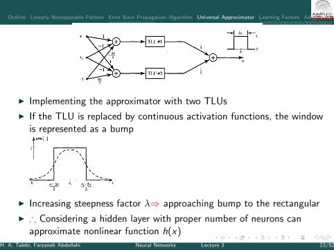
I Implementing the approximator with two TLUs
I If the TLU is replaced by continuous activation functions, the windowis represented as a bump
I Increasing steepness factor λ⇒ approaching bump to the rectangular
I ∴ Considering a hidden layer with proper number of neurons canapproximate nonlinear function h(x)
H. A. Talebi, Farzaneh Abdollahi Neural Networks Lecture 3 23/52
Outline Linearly Nonseparable Pattern Error Back Propagation Algorithm Universal Approximator Learning Factors Adaptive MLP
Multilayer NN as Universal Approximator
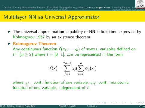
I The universal approximation capability of NN is first time expressed byKolmogorov 1957 by an existence theorem.
I Kolmogorov TheoremAny continuous function f (x1, ..., xn) of several variables defined onI n (n ≥ 2) where I = [0 1], can be represented in the form
f (x) =2n+1∑j=1
χj(n∑
i=1
ψij(xi )
where χj : cont. function of one variable, ψij : cont. monotonicfunction of one variable, independent of f .
H. A. Talebi, Farzaneh Abdollahi Neural Networks Lecture 3 24/52
Outline Linearly Nonseparable Pattern Error Back Propagation Algorithm Universal Approximator Learning Factors Adaptive MLP
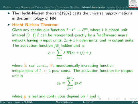
I The Hecht-Nielsen theorem(1987) casts the universal approximationsin the terminology of NN
I Hecht-Nielsen Theorem:Given any continuous function f : I n → Rm, where I is closed unitinterval [0 1] f can be represented exactly by a feedforward neuralnetwork having n input units, 2n + 1 hidden units, and m output units.The activation function jth hidden unit is
zj =n∑
i=1
λiΨ(xi + εj) + j
where λ: real const., Ψ: monotonically increasing functionindependent of f , ε: a pos. const. The activation function for outputunit is
yk =2n+1∑j=1
gkzj
where g is real and continuous depend on f and ε.H. A. Talebi, Farzaneh Abdollahi Neural Networks Lecture 3 25/52
Outline Linearly Nonseparable Pattern Error Back Propagation Algorithm Universal Approximator Learning Factors Adaptive MLP
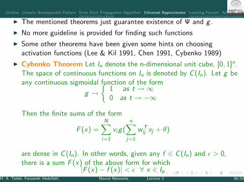
I The mentioned theorems just guarantee existence of Ψ and g .
I No more guideline is provided for finding such functions
I Some other theorems have been given some hints on choosingactivation functions (Lee & Kil 1991, Chen 1991, Cybenko 1989)
I Cybenko Theorem Let In denote the n-dimensional unit cube, [0, 1]n.The space of continuous functions on In is denoted by C (In). Let g beany continuous sigmoidal function of the form
g →{
1 as t →∞0 as t → −∞
Then the finite sums of the form
F (x) =N∑
i=1
vig(n∑
j=1
wTij xj + θ)
are dense in C (In). In other words, given any f ∈ C (In) and ε > 0,there is a sum F (x) of the above form for which
|F (x)− f (x)| < ε ∀ x ∈ InH. A. Talebi, Farzaneh Abdollahi Neural Networks Lecture 3 26/52
Outline Linearly Nonseparable Pattern Error Back Propagation Algorithm Universal Approximator Learning Factors Adaptive MLP
I MLP can provide all the conditions of Cybenko theoremI θ is biasI wij is weights of input layerI vi is output layer weights
I Failures in approximation can be attribute toI Inadequate learningI Inadequate # of hidden neuronsI Lack of deterministic relationship between the input and target output
I If the function to be approximated is not bounded, there is noguarantee for acceptable approximation
H. A. Talebi, Farzaneh Abdollahi Neural Networks Lecture 3 27/52
Outline Linearly Nonseparable Pattern Error Back Propagation Algorithm Universal Approximator Learning Factors Adaptive MLP
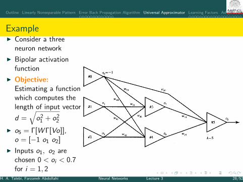
ExampleI Consider a three
neuron network
I Bipolar activationfunction
I Objective:Estimating a functionwhich computes thelength of input vector
d =√
o21 + o2
2
I o5 = Γ[W Γ[Vo]],o = [−1 o1 o2]
I Inputs o1, o2 arechosen 0 < oi < 0.7for i = 1, 2
H. A. Talebi, Farzaneh Abdollahi Neural Networks Lecture 3 28/52

Outline Linearly Nonseparable Pattern Error Back Propagation Algorithm Universal Approximator Learning Factors Adaptive MLP
Example Cont’d, Experiment 1
I Using 10 training points which areinformally spread in lower half of firstplane
I The training is stopped at error 0.01 after2080 steps
I η = 0.2
I The weights are W = [0.03 3.66 2.73]T ,
V =
[−1.29 −3.04 −1.540.97 2.61 0.52
]I Magnitude of error associated with each
training pattern are shown on the surface
I Any generalization provided by trainednetwork is questionable.
H. A. Talebi, Farzaneh Abdollahi Neural Networks Lecture 3 29/52
Outline Linearly Nonseparable Pattern Error Back Propagation Algorithm Universal Approximator Learning Factors Adaptive MLP
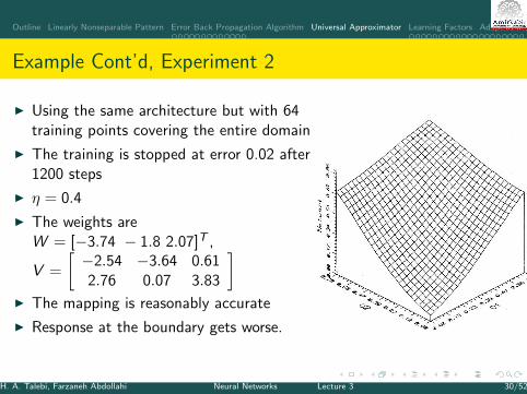
Example Cont’d, Experiment 2
I Using the same architecture but with 64training points covering the entire domain
I The training is stopped at error 0.02 after1200 steps
I η = 0.4
I The weights areW = [−3.74 − 1.8 2.07]T ,
V =
[−2.54 −3.64 0.612.76 0.07 3.83
]I The mapping is reasonably accurate
I Response at the boundary gets worse.
H. A. Talebi, Farzaneh Abdollahi Neural Networks Lecture 3 30/52
Outline Linearly Nonseparable Pattern Error Back Propagation Algorithm Universal Approximator Learning Factors Adaptive MLP
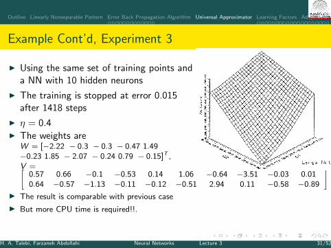
Example Cont’d, Experiment 3
I Using the same set of training points anda NN with 10 hidden neurons
I The training is stopped at error 0.015after 1418 steps
I η = 0.4I The weights are
W = [−2.22 − 0.3 − 0.3 − 0.47 1.49−0.23 1.85 − 2.07 − 0.24 0.79 − 0.15]T ,V =[
0.57 0.66 −0.1 −0.53 0.14 1.06 −0.64 −3.51 −0.03 0.010.64 −0.57 −1.13 −0.11 −0.12 −0.51 2.94 0.11 −0.58 −0.89
]I The result is comparable with previous case
I But more CPU time is required!!.
H. A. Talebi, Farzaneh Abdollahi Neural Networks Lecture 3 31/52
Outline Linearly Nonseparable Pattern Error Back Propagation Algorithm Universal Approximator Learning Factors Adaptive MLP
Initial WeightsI They are usually selected at small random values. (between -1 and 1
or -0.5 and 0.5)
I They affect finding local/global min and speed of convergence
I Choosing them too large saturates network and terminates learning
I Choosing them too small decreases the learning rate.
I They should be chosen s.t do not make the activation function or itsderivative zero
I If all weights start with equal values, the network may not trainproperly.
I Some improper inial weights may result in increasing the errors anddecreasing the quality of mapping.
I At these cases the network learning should be restarted with newrandom weights.
H. A. Talebi, Farzaneh Abdollahi Neural Networks Lecture 3 32/52
Outline Linearly Nonseparable Pattern Error Back Propagation Algorithm Universal Approximator Learning Factors Adaptive MLP
Error
I The training is based on min error
I In delta rule algorithm, Cumulative error is calculatedE = 1
2
∑Pp=1
∑Rk=1(dpk − opk)2
I Sometimes it is recommended to use Erms = 1pk
√(dpk − opk)2
I If output should be discrete (like classification), activation function ofoutput layer is chosen TLU, so the error is
Ed =Nerr
pk
where Nerr : # bit errors, p: # training patterns, and k # outputs.
I Emax for discrete output can be zero, but in continuous output maynot be.
H. A. Talebi, Farzaneh Abdollahi Neural Networks Lecture 3 33/52
Outline Linearly Nonseparable Pattern Error Back Propagation Algorithm Universal Approximator Learning Factors Adaptive MLP
Training versus Generalization
I If learning takes long, network losses the generalization capability. Inthis case it is said, the network memorizes the training patterns
I To ovoid this problem, Hecht-Nielsen (1990) introducestraining-testing pattern (T.T,P)
I Some specific patterns named T.T.P is applied during training period.I If the error obtained by applying the T.T.P is decreasing, the training
can be continued.I Otherwise, the training is terminated to avoid memorization.
H. A. Talebi, Farzaneh Abdollahi Neural Networks Lecture 3 34/52
Outline Linearly Nonseparable Pattern Error Back Propagation Algorithm Universal Approximator Learning Factors Adaptive MLP
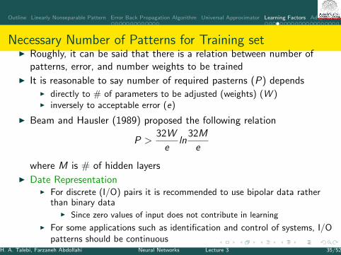
Necessary Number of Patterns for Training setI Roughly, it can be said that there is a relation between number of
patterns, error, and number weights to be trainedI It is reasonable to say number of required pasterns (P) depends
I directly to # of parameters to be adjusted (weights) (W )I inversely to acceptable error (e)
I Beam and Hausler (1989) proposed the following relation
P >32W
eln
32M
e
where M is # of hidden layersI Date Representation
I For discrete (I/O) pairs it is recommended to use bipolar data ratherthan binary data
I Since zero values of input does not contribute in learning
I For some applications such as identification and control of systems, I/Opatterns should be continuous
H. A. Talebi, Farzaneh Abdollahi Neural Networks Lecture 3 35/52
Outline Linearly Nonseparable Pattern Error Back Propagation Algorithm Universal Approximator Learning Factors Adaptive MLP
Necessary Number of Hidden Neurons
I There is no clear and exact rule due to complexity of the networkmapping and nondeterministic nature of many successfully completedtraining procedure.
I # neurons depends on the function to be approximated.I Its degree of nonlinearity affects the size of network
I Note that considering large number of neurons and layers may causeoverfitting and decrease the generalization capability
I Number of Hidden LayersI Based on the universal approximation theorem one hidden layer is
sufficient for a BP to approximate any continuous mapping from theinput patterns to the output patterns to an arbitrary degree of accuracy.
I More hidden layers may make training easier in some situations or toocomplicated to converge.
H. A. Talebi, Farzaneh Abdollahi Neural Networks Lecture 3 36/52
Outline Linearly Nonseparable Pattern Error Back Propagation Algorithm Universal Approximator Learning Factors Adaptive MLP
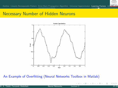
Necessary Number of Hidden Neurons
An Example of Overfitting (Neural Networks Toolbox in Matlab)
H. A. Talebi, Farzaneh Abdollahi Neural Networks Lecture 3 37/52
Outline Linearly Nonseparable Pattern Error Back Propagation Algorithm Universal Approximator Learning Factors Adaptive MLP
Learning Constant
I Obviously, convergence of error BP alg. depends on the value of η
I In general, optimum value of η depends o the problem to be solved
I When broad minima yields small gradient values, larger η makes theconvergence more rapid.
I For steep and narrow minima, small value of η avoids overshootingand oscillation.
I ∴ η should be chosen experimentally for each problem
I Several methods has been introduced to adjust learning const. (η).
I Adaptive Learning Rate in MATLAB adjusts η based onincreasing/decreasing error
H. A. Talebi, Farzaneh Abdollahi Neural Networks Lecture 3 38/52

Outline Linearly Nonseparable Pattern Error Back Propagation Algorithm Universal Approximator Learning Factors Adaptive MLP
I η can be defined exponentially,
I At first steps it is large
I By increasing number of steps and getting closer to minima itbecomes smaller.
H. A. Talebi, Farzaneh Abdollahi Neural Networks Lecture 3 39/52
Outline Linearly Nonseparable Pattern Error Back Propagation Algorithm Universal Approximator Learning Factors Adaptive MLP
Delta-Bar-Delta
I For each weight a different η is specified
I If updating the weight is in the same direction (increasing/decreasing)in some sequential steps, η is increased
I Otherwise η should decrease
I The updating rule for weight is: wij(n + 1) = wij(n)− ηij(n + 1) ∂E(n)∂wij (n)
I The learning rate can be updated based on the following rule:
ηij(n + 1) = −γ ∂E (n)
∂ηij(n)
I where ηij is learning rate corresponding to weights of output layer wij .
I It can be shown that learning rate is updated based on wij as follows
(Show it as exercise) ηij(n + 1) = −γ ∂E(n)∂wij (n) .
∂E(n−1)∂wij (n−1)
H. A. Talebi, Farzaneh Abdollahi Neural Networks Lecture 3 40/52
Outline Linearly Nonseparable Pattern Error Back Propagation Algorithm Universal Approximator Learning Factors Adaptive MLP
Momentum methodI This method accelerates the convergence of error BP
I Generally, if the training data are not accurate, the weights oscillateand cannot converge to their optimum values
I In momentum method, the speed of BP error convergence is increasedwithout changing η
I In this method, the current weight adjustment confiders a fraction ofthe most recent weight 4w(t) = −η∇E (t) + α4w(t − 1)where α is pos, const. named momentum const.
I The second term is called momentum term
I If the gradients in two consecutive steps have the same sign, themomentum term is pos. and the weight changes more
I Otherwise, the weights are changed less, but in direction ofmomentum
I ∴ its direction is correctedH. A. Talebi, Farzaneh Abdollahi Neural Networks Lecture 3 41/52

Outline Linearly Nonseparable Pattern Error Back Propagation Algorithm Universal Approximator Learning Factors Adaptive MLP
I Start form A’
I Gradient of A’ and A” have the samesigns
I ∴ the convergence speeds up
I Now start form B’
I Gradient of B’ and B” have the differentsigns
I ∂E∂w2
does not point to min
I adding momentum term corrects thedirection towards min
I ∴ If the gradient in two consecutive stepchanges the sign, the learning const.should decrease in those directions(Jacobs 1988)
H. A. Talebi, Farzaneh Abdollahi Neural Networks Lecture 3 42/52
Outline Linearly Nonseparable Pattern Error Back Propagation Algorithm Universal Approximator Learning Factors Adaptive MLP
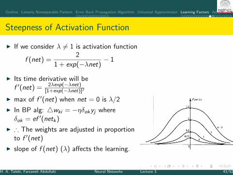
Steepness of Activation Function
I If we consider λ 6= 1 is activation function
f (net) =2
1 + exp(−λnet)− 1
I Its time derivative will bef ′(net) = 2λexp(−λnet)
[1+exp(−λnet)]2
I max of f ′(net) when net = 0 is λ/2
I In BP alg: 4wki = −ηδokyj whereδok = ef ′(netk)
I ∴ The weights are adjusted in proportionto f ′(net)
I slope of f (net) (λ) affects the learning.
H. A. Talebi, Farzaneh Abdollahi Neural Networks Lecture 3 43/52
Outline Linearly Nonseparable Pattern Error Back Propagation Algorithm Universal Approximator Learning Factors Adaptive MLP
I The weights connected to the units responding in their mid-range arechanged the most
I The units which are saturated change less.
I In some MLP, the learning constant is fixed and by adapting λaccelerate the error convergence (Rezgui 1991).
I But most commonly, λ = 1 are fixed and the learning speed iscontrolled by η
H. A. Talebi, Farzaneh Abdollahi Neural Networks Lecture 3 44/52
Outline Linearly Nonseparable Pattern Error Back Propagation Algorithm Universal Approximator Learning Factors Adaptive MLP
Batch versus Incremental UpdatesI Incremental updating: a small weights adjustment follows after each
presentation of the training pattern.I disadvantage: The network trained this way, may be skewed toward the
most recent patterns in the cycle.
I Batch updating: accumulate the weight correction terms for severalpatterns (or even an entire epoch (presenting all patterns)) and makea single weight adjustment equal to the average of the weightcorrection terms:
4w =P∑
p=1
4wp
I disadvantages: This procedure has a smoothing effect on the correctionterms which in some cases, it increases the chances of convergence to alocal min.
H. A. Talebi, Farzaneh Abdollahi Neural Networks Lecture 3 45/52
Outline Linearly Nonseparable Pattern Error Back Propagation Algorithm Universal Approximator Learning Factors Adaptive MLP
Normalization
I IF I/O patterns are distributed in a wide range, it is recommended tonormalize them before use for training.
I Recall time derivative of sigmoid activation fcn:
f ′(net) =
{o(1− o) unipolar : f (net) = 1
1+exp(−λnet) , λ = 112(1− o2) bipolar : f (net) = 2
1+exp(−λnet) − 1, λ = 1
I It appears in δ for updating the weights.
I If output of sigmoid fcn gets to the saturation area, (1 or -1) due tolarge values of weights or not normalized input data f ′(net)→ 0and δ → 0. So the weight updating is stopped.
I I/O normalization will increases the chance of convergence to theacceptable results.
H. A. Talebi, Farzaneh Abdollahi Neural Networks Lecture 3 46/52
Outline Linearly Nonseparable Pattern Error Back Propagation Algorithm Universal Approximator Learning Factors Adaptive MLP
Offline versus Online Training
I Offline training :I After the weights converge to the desired values and learning is
terminated, the trained feed forward network is employedI When enough data is available for training and no unpredicted behavior
is expected from the system, offline training is recommended.
I Online training:I Updating the weights and performing the network is simultaneously.I In online training NN can adapt itself with unpredicted changing
behavior of the system.I The weights convergence should be fast to avoid undesired performance.I For exp. if NN is employed as a controller and is not trained fast, it
may lead to instabilityI If there is enough data it is suggested to train NN offline and use the
trained weight as initial weights in online training to facilitate thetraining
H. A. Talebi, Farzaneh Abdollahi Neural Networks Lecture 3 47/52
Outline Linearly Nonseparable Pattern Error Back Propagation Algorithm Universal Approximator Learning Factors Adaptive MLP
Levenberg-Marquardt Training [?]I The LevenbergMarquardt algorithm (LMA) provides a numerical
solution to the problem of minimizing a function
I It interpolates between the GaussNewton algorithm (GNA) andgradient descent method.
I The LMA is more robust than the GNA,I It will end the solution even if the initial values are very far off the final
minimum.
I In many cases LMA converges faster than gradient decent method.
I LMA is a compromise between the speed of GNA and guaranteedconvergence of gradient alg. decent
I Recall the error is defined as sum of squares function forE = 1
2ΣKk=1ΣP
p=1e2pk , epk = dpk − opk
I The learning rule based on gradient decent alg is ∆wkj = −η ∂E∂wkj
H. A. Talebi, Farzaneh Abdollahi Neural Networks Lecture 3 48/52
Outline Linearly Nonseparable Pattern Error Back Propagation Algorithm Universal Approximator Learning Factors Adaptive MLP
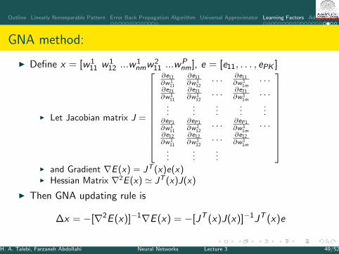
GNA method:
I Define x = [w111 w1
12 ...w1nmw2
11 ...wPnm], e = [e11, . . . , ePK ]
I Let Jacobian matrix J =
∂e11
∂w111
∂e11
∂w112
. . . ∂e11
∂w11m
. . .∂e21
∂w111
∂e21
∂w112
. . . ∂e21
∂w11m
. . .
......
......
...∂eP1
∂w111
∂eP1
∂w112
. . . ∂eP1
∂w11m
. . .∂e12
∂w111
∂e12
∂w112
. . . ∂e12
∂w11m
......
...
I and Gradient ∇E (x) = JT (x)e(x)I Hessian Matrix ∇2E (x) ' JT (x)J(x)
I Then GNA updating rule is
∆x = −[∇2E (x)]−1∇E (x) = −[JT (x)J(x)]−1JT (x)e
H. A. Talebi, Farzaneh Abdollahi Neural Networks Lecture 3 49/52
Outline Linearly Nonseparable Pattern Error Back Propagation Algorithm Universal Approximator Learning Factors Adaptive MLP
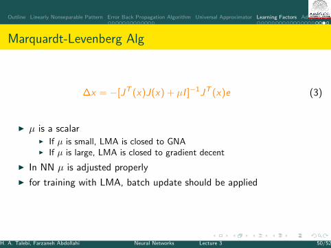
Marquardt-Levenberg Alg
∆x = −[JT (x)J(x) + µI ]−1JT (x)e (3)
I µ is a scalarI If µ is small, LMA is closed to GNAI If µ is large, LMA is closed to gradient decent
I In NN µ is adjusted properly
I for training with LMA, batch update should be applied
H. A. Talebi, Farzaneh Abdollahi Neural Networks Lecture 3 50/52
Outline Linearly Nonseparable Pattern Error Back Propagation Algorithm Universal Approximator Learning Factors Adaptive MLP
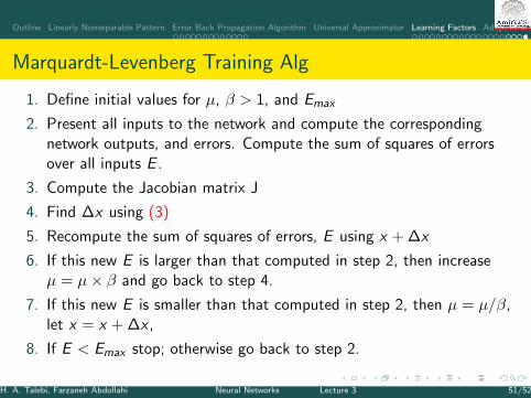
Marquardt-Levenberg Training Alg
1. Define initial values for µ, β > 1, and Emax
2. Present all inputs to the network and compute the correspondingnetwork outputs, and errors. Compute the sum of squares of errorsover all inputs E .
3. Compute the Jacobian matrix J
4. Find ∆x using (3)
5. Recompute the sum of squares of errors, E using x + ∆x
6. If this new E is larger than that computed in step 2, then increaseµ = µ× β and go back to step 4.
7. If this new E is smaller than that computed in step 2, then µ = µ/β,let x = x + ∆x ,
8. If E < Emax stop; otherwise go back to step 2.
H. A. Talebi, Farzaneh Abdollahi Neural Networks Lecture 3 51/52
Outline Linearly Nonseparable Pattern Error Back Propagation Algorithm Universal Approximator Learning Factors Adaptive MLP
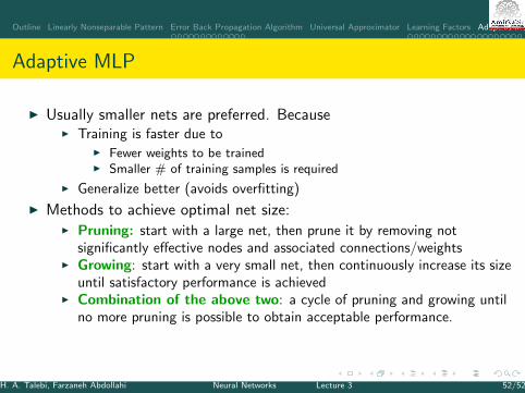
Adaptive MLP
I Usually smaller nets are preferred. BecauseI Training is faster due to
I Fewer weights to be trainedI Smaller # of training samples is required
I Generalize better (avoids overfitting)
I Methods to achieve optimal net size:I Pruning: start with a large net, then prune it by removing not
significantly effective nodes and associated connections/weightsI Growing: start with a very small net, then continuously increase its size
until satisfactory performance is achievedI Combination of the above two: a cycle of pruning and growing until
no more pruning is possible to obtain acceptable performance.
H. A. Talebi, Farzaneh Abdollahi Neural Networks Lecture 3 52/52