Embed Size (px)
Citation preview
Technical Report HL-95-5 September 1995
US Army Corps of Engineers Waterways Experiment Station
FEMWATER Usability for the EPA MASTER and Wellhead Protection Research Programs
by Hsin-Chi Jerry Lin, Patrick Deliman, William D. Martin
EUECTE kWM offliaa
Approved For Public Release; Distribution is Unlimited
19951106 019
*n!
«»**? * T^te
&
•%*** v» -\"
DTie QUALITY INSPECTED 8
Prepared for U.S. Environmental Protection Agency Environmental Research Laboratory
The contents of this report are not to be used for advertising, publication, or promotional purposes. Citation of trade names does not constitute an official endorsement or approval of the use of such commercial products.
€J7 PRINTED ON RECYCLED PAPER

DISCLÄIME1 NOTICE
THIS DOCUMENT IS BEST
QUALITY AVAILABLE. THE COPY
FURNISHED TO DTIC CONTAINED
A SIGNIFICANT NUMBER OF
COLOR PAGES WHICH DO NOT
REPRODUCE LEGIBLY ON BLACK
AND WHITE MICROFICHE.
Technical Report HL-95-5 September 1995
FEMWATER Usability for the EPA MASTER Wellhead Protection Research Programs by Hsin-Chi Jerry Lin, Patrick Deliman, William D. Martin
U.S. Army Corps of Engineers Waterways Experiment Station 3909 Halls Ferry Road Vicksburg, MS 39180-6199
Final report Approved for public release; distribution is unlimited
Prepared for U.S. Environmental Protection Agency Environmental Research Laboratory Athens, GA 30605
in ill lul-
US Army Corps of Engineers Waterways Experiment Station
KEAD0UAKTB6 ■JLOttG
OCNTACT:
PUBLIC AFFAIRS OFFICE
U.S. ARMY ENGINEER WATERWAYS EXPERMENT STATION MB HALLS FERRY ROAD VEKSBURQ, WSSSSPPI K1I0«1M
PHONE: (anics4-2n2
Waterways Experiment Station Cataloging-in-Publication Data
Lin, Hsin-Chi Jerry. FEMWATER usability for the EPA MASTER and Wellhead Protection
Research Programs / by Hsin-Chi Jerry Lin, Patrick Deliman, William D. Martin ; prepared for U.S. Environmental Protection Agency, Environ- mental Research Laboratory.
92 p.: ill.; 28 cm. — (Technical report; HL-95-5) 1. Groundwater — Mathematical models. 2. Watersheds — Iowa.
3. Groundwater —Pollution — Mathematical models. 4. Porous materials. I. Deliman, Patrick. II. Martin, William D. III. United States. Army. Corps of Engineers. IV. U.S. Army Engineer Waterways Experi- ment Station. V. Hydraulics Laboratory (U.S. Army Engineer Waterways Experiment Station) VI. United States. Environmental Protection Agency. VII. Environmental Research Laboratory (Athens, Ga.) VIII. Title. IX. Series: Technical report (U.S. Army Engineer Waterways Experiment Station); HL-95-5. TA7 W34 no.HL-95-5
Contents
Preface vi
1—Introduction 1
Walnut Creek Watershed 1 Objectives 3 Scope of Study 3
2—Data Collection 5
Digital Elevation Data 5 Geology 5 Driller's Logs of Shallow Observation Wells 6 Precipitation and Interior Wells 6 Drain Tiles and Tile Flow . 10 Subwatershed Boundaries 10
3—3-D Mesh Construction 16
2-D Surface Mesh 16 3-D Mesh 16
4—Flow Simulation 29
Simulated Flow for Inset Mesh 30 Simulated Flow for Entire Watershed 35
5—Preliminary Exposure Assessment 41
General Description 41 Parameter Development 41 Simulation Results 46
6—Sensitivity Analysis 52
General Description 52 Analysis Protocol 52 Simulation Results 52
7—Summary and Conclusions 87
References 89
SF298
in
List of Figures
Figure 1. Location map of Walnut Creek watershed 2
Figure 2. Data available map in Walnut Creek watershed 4
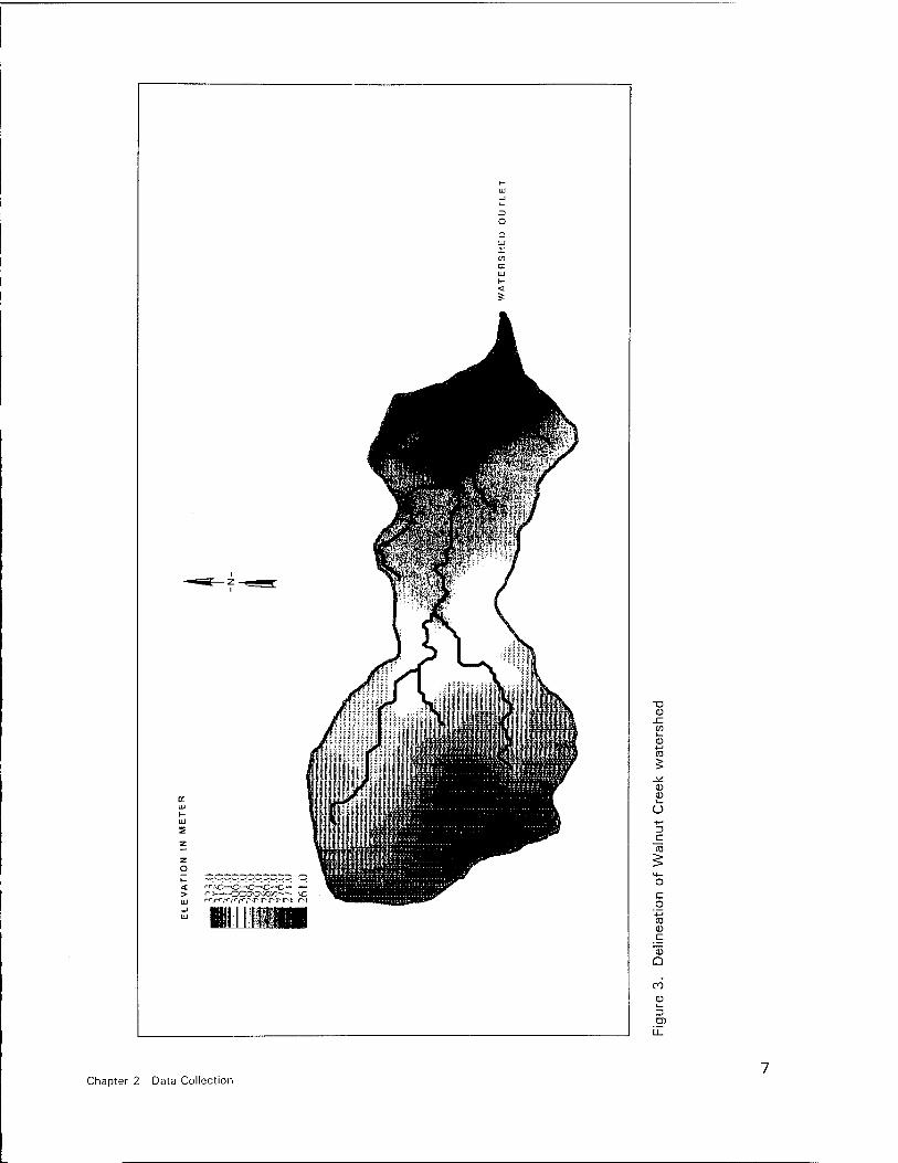
Figure 3. Delineation of Walnut Creek watershed 7
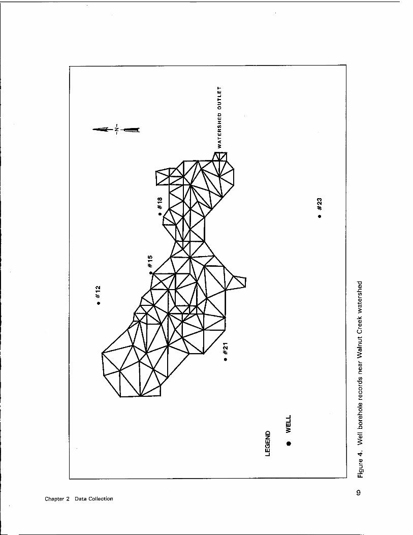
Figure 4. Well borehole records near Walnut Creek watershed 9
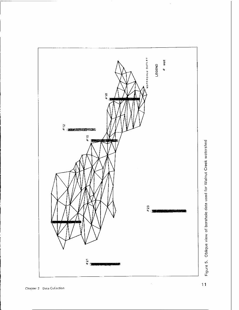
Figure 5. Oblique view of borehole data used for Walnut Creek watershed 11
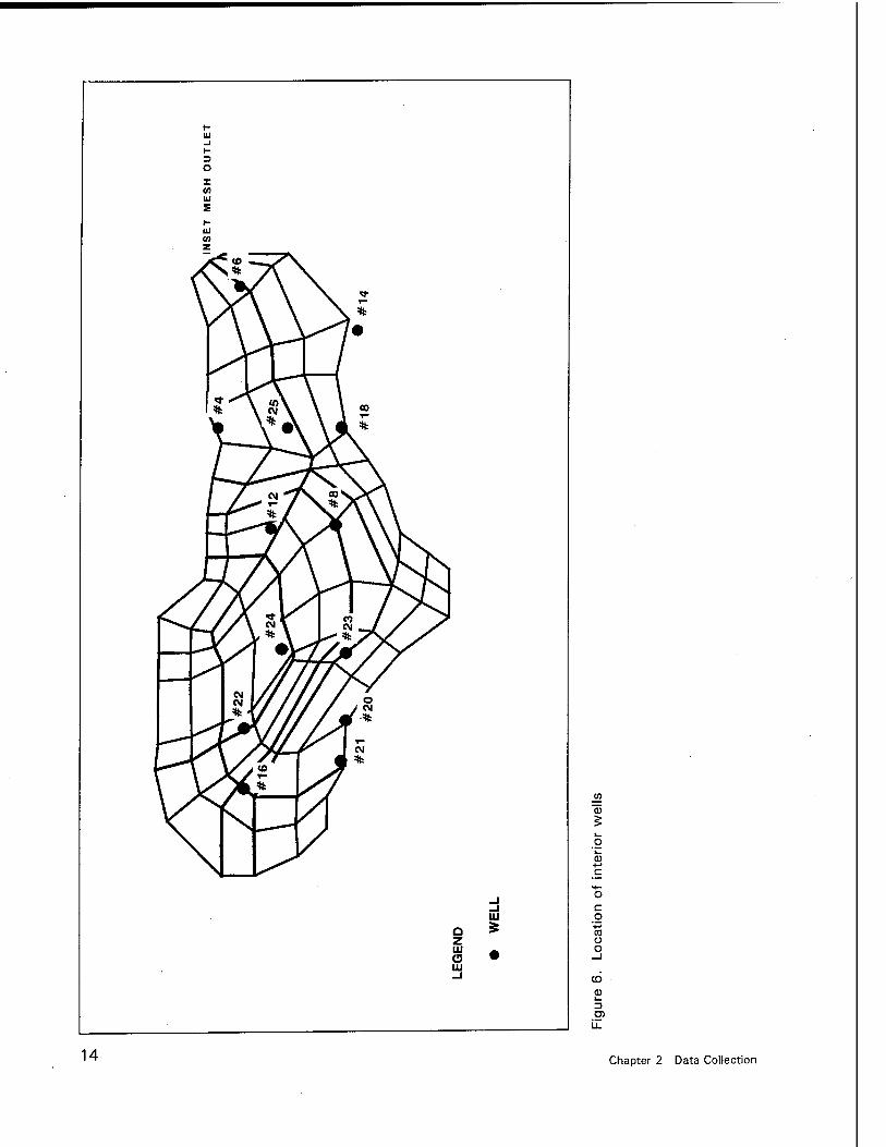
Figure 6. Location of interior wells 14
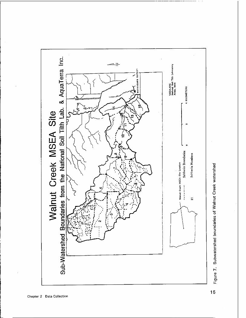
Figure 7. Subwatershed boundaries of Walnut Creek watershed 15
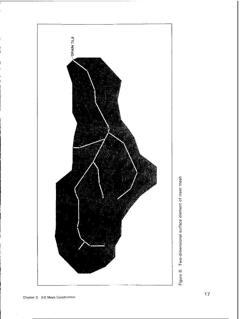
Figure 8. Two-dimensional surface element of inset mesh 17
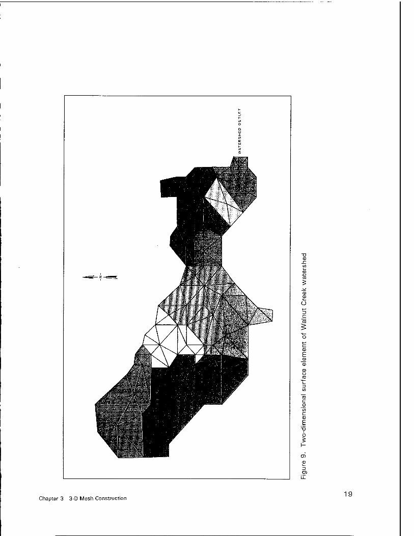
Figure 9. Two-dimensional surface element of Walnut Creek watershed . . 19
Figure 10. Three-dimensional mesh of inset mesh of Walnut Creek watershed 23
Figure 11. Drain tile location at the bottom of inset mesh 25
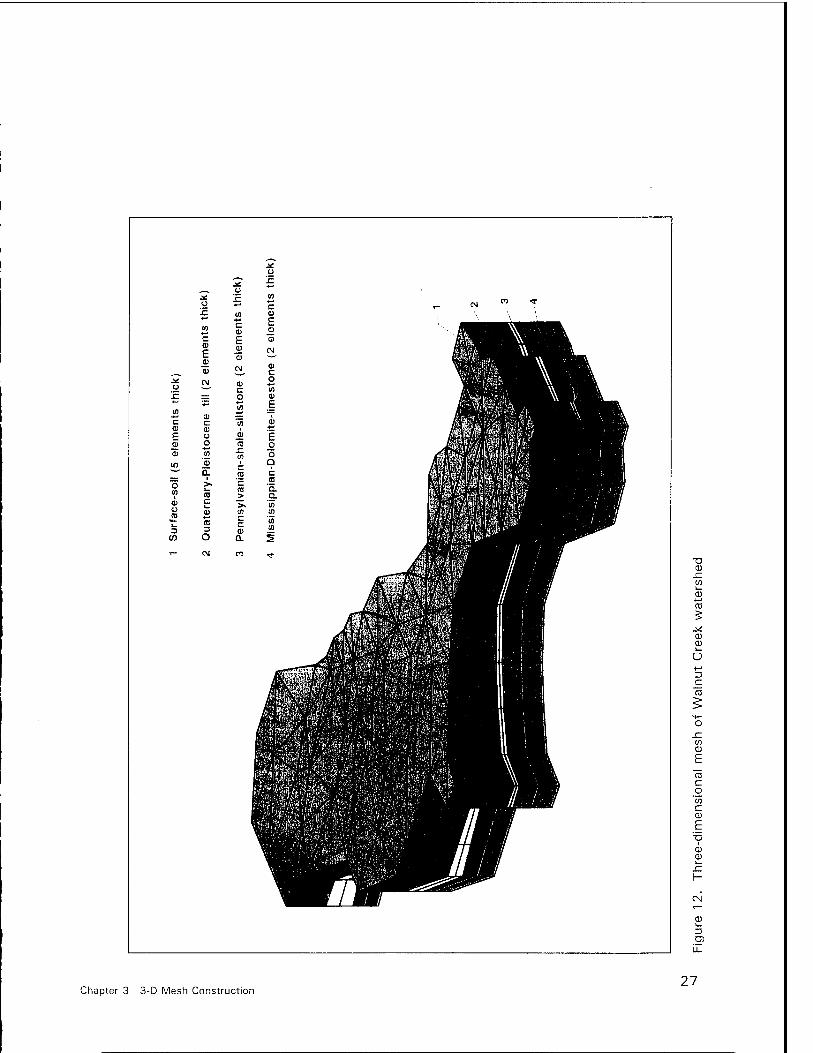
Figure 12. Three-dimensional mesh of Walnut Creek watershed 27
Figure 13. Assignment of Dirichlet boundary on the boundary nodes .... 31
Figure 14. Spatial rainfall distribution of inset mesh 37
Figure 15. Simulated flow pattern in the second layer of the surface soil for the 966-hr time-step 39
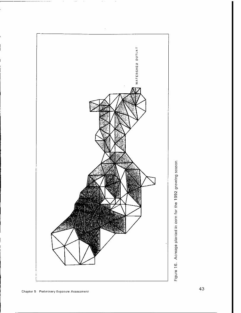
Figure 16. Acreage planted in corn for the 1992 growing season 43
Figure 17. Atrazine concentrations in the second layer of the surface soil at time 966 hr 47
Figure 18. Atrazine concentrations in the second layer of the surface soil at time 1056 hr 49
Figure 19. Distribution of corn acreage for alternative land- use simulation 53
Figure 20. Atrazine concentrations with alternative land-use scheme at time 966 hr 57
Figure 21. Atrazine concentrations with alternative land-use scheme at time 1056 hr 59
Figure 22. Atrazine concentrations with alternative land-use scheme at time 1161 hr 61
Figure 23. Atrazine concentrations from maximum conductivity at time 966 hr 63
IV
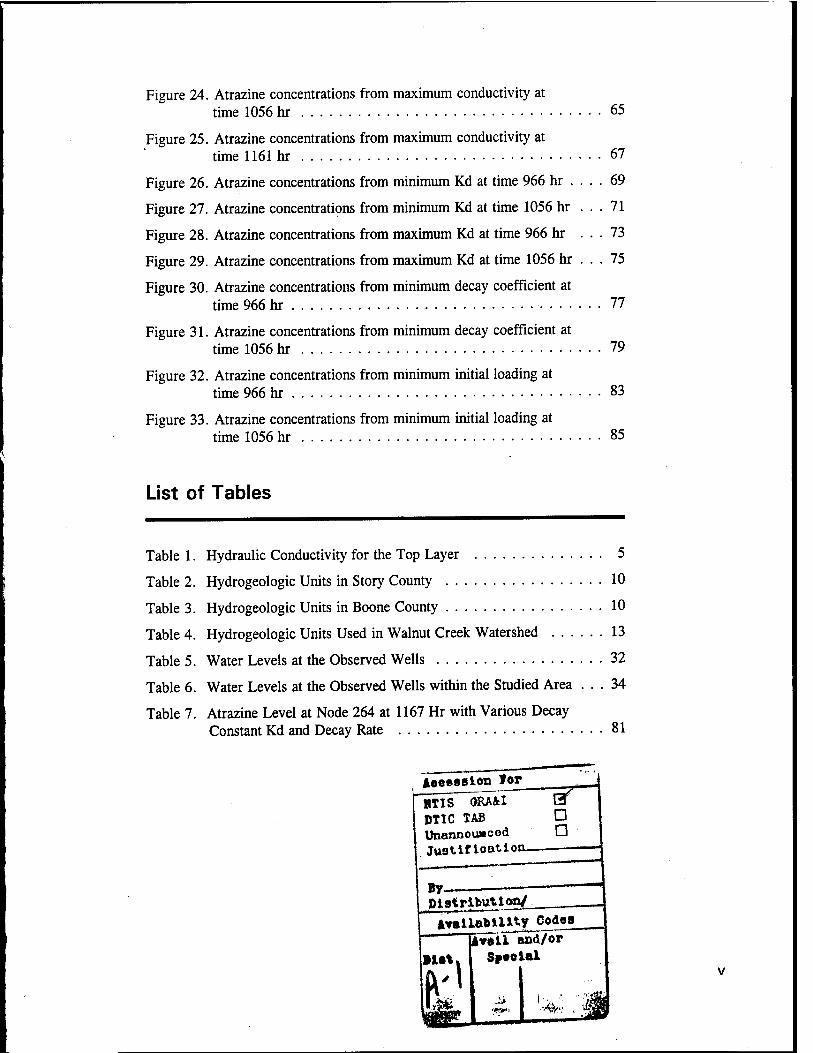
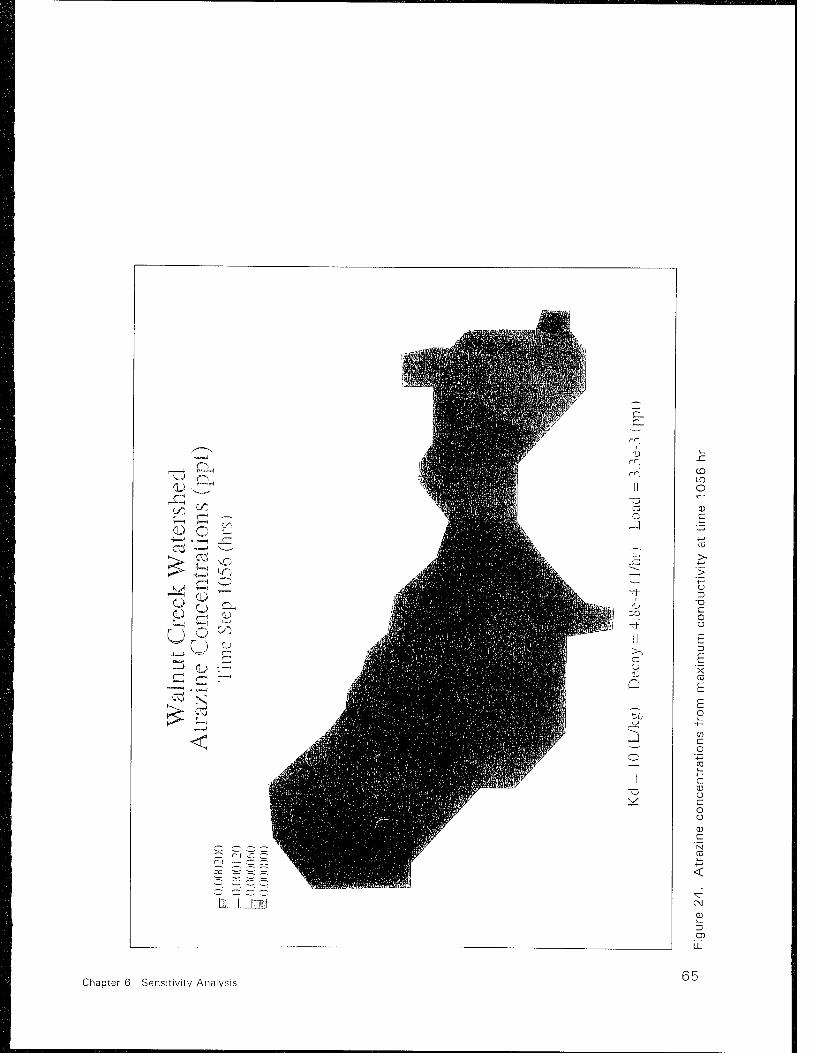
Figure 24. Atrazine concentrations from maximum conductivity at time 1056 hr 65
Figure 25. Atrazine concentrations from maximum conductivity at time 1161 hr 67
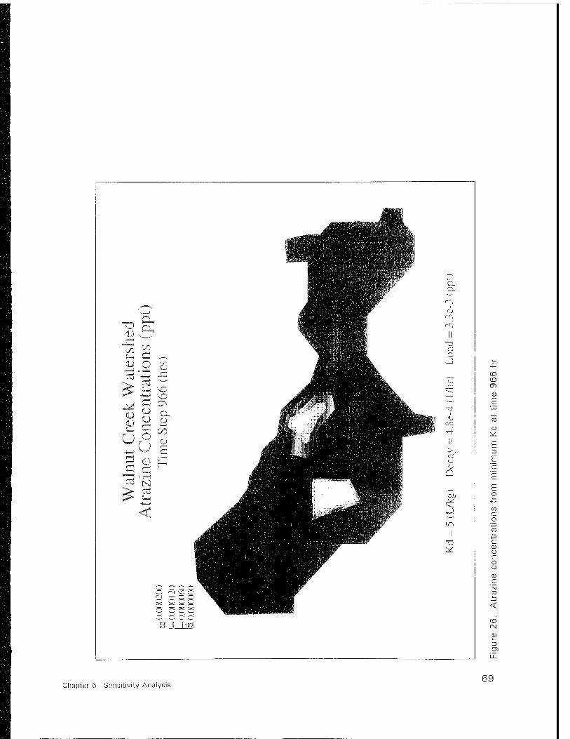
Figure 26. Atrazine concentrations from minimum Kd at time 966 hr .... 69
Figure 27. Atrazine concentrations from minimum Kd at time 1056 hr ... 71
Figure 28. Atrazine concentrations from maximum Kd at time 966 hr ... 73
Figure 29. Atrazine concentrations from maximum Kd at time 1056 hr . . . 75
Figure 30. Atrazine concentrations from minimum decay coefficient at time 966 hr 77
Figure 31. Atrazine concentrations from minimum decay coefficient at time 1056 hr 79
Figure 32. Atrazine concentrations from minimum initial loading at time 966 hr 83
Figure 33. Atrazine concentrations from minimum initial loading at time 1056 hr 85
List of Tables
Table 1. Hydraulic Conductivity for the Top Layer 5
Table 2. Hydrogeologie Units in Story County 10
Table 3. Hydrogeologie Units in Boone County 10
Table 4. Hydrogeologie Units Used in Walnut Creek Watershed 13
Table 5. Water Levels at the Observed Wells 32
Table 6. Water Levels at the Observed Wells within the Studied Area ... 34
Table 7. Atrazine Level at Node 264 at 1167 Hr with Various Decay Constant Kd and Decay Rate 81
Accession Tor
ITIS ORMI DTIC TAB Unannounced Justlf icatlon.
By Distribute oa/
a a
AwiiöMlltyJJoäe«. frill and/or
Special v
Preface
The FEMWATER Usability for the EPA MASTER Wellhead Protection Research Programs study, as documented in this report, was performed for the U.S. Environmental Protection Agency EPA Environmental Research Laboratory, Athens, GA. Dr. Bob Carsel, EPA Athens Environmental Research Laboratory, was point of contact.
The study was conducted in the Hydraulics Laboratory (HL) and Environmental Laboratory (EL) of the U.S. Army Engineer Waterways Experiment Station (WES) during the period December 1992 to September 1994 under the direction of Messers. F. A. Herrmann, Jr., Director, HL; R. A. Sager, Assistant Director, HL; W. H. McAnally, Jr., Chief, Estuaries Division (ED), HL; and W. D. Martin, Chief, Estuarine Engineering Branch (EEB), ED; and Dr. John Harrison, Director, EL; Dr. John W. Keeley, Assistant Director, EL; Mr. D. L. Robey, Chief, Environmental Processes and Effects Division, EL; and Dr. M. S. Dortch, Chief, Water Quality and Contaminant Modeling Branch (WQCMB), Environmental Processes and Effects Division.
The study was conducted by Dr. Hsin-Chi J. Lin, EEB, and Dr. Patrick Deliman, WQCMB, and the report was prepared by Drs. Lin and Deliman and Mr. Martin.
Dr. Robert W. Whalin was Director of WES during the publication of this report. COL Bruce K. Howard, EN, was Commander.
The contents of this report are not to be used for advertising, publication, or promotional purposes. Citation of trade names does not constitute an official endorsement or approval of the use of such commercial products.
VI
1 Introduction
The U. S. Army Engineer Waterways Experiment Station (WES) and Brigham Young University (BYU) have jointly developed a user-friendly graphical interface for groundwater models, the Groundwater Modeling System (GMS). The GMS (BYU 1994a) is a pre- and post-processing soft- ware for several different groundwater models, including a three-dimensional finite element model of density-dependent flow and transport through saturated-unsaturated porous media (FEMWATER). The model was devel- oped by G.T. (George) Yeh, Pennsylvania State University (PSU). The model stems from two pervious codes, a groundwater flow model (3DFEMWATER) and a subsurface contaminant transport model (3DLEWASTE). The FEMWATER can handle all the options of the two previous models plus the option of density-driven flow and transport. The input and output structures of the model have been modified by WES to adapt the graphical interface file format. The documentation of FEMWATER user's manual has been published by WES (Lin and Yeh 1995). The documentation of FEMWATER provides the formulation, the input data files, and some sample problems for the FEMWATER model. This subject of study is a cooperative research effort between the U. S. Environmental Protection Agency (EPA) Environmental Research Laboratory at Athens, GA (AERL), WES, and PSU. The Walnut Creek watershed near Ames, IA, was selected to demonstrate the usability of this tool. This watershed is the site of a multi- agency effort to collect comprehensive field data covering geometry, geology, surface water, and agricultural chemical profile characteristics.
Walnut Creek Watershed
Walnut Creek watershed (Figure 1) located within Boone and Story Counties of central Iowa is characterized by a gently rolling topography with a relatively thin weathered, sandy till near the surface. Walnut Creek traverses rolling hills along the route from its upper reaches near the community of Kelly flowing southeastward to its confluence with the South Skunk River below the city of Ames. The drainage area of the watershed is approximately 5,000 ha. The watershed is near level with numerous potholes in the upper
Chapter 1 Introduction
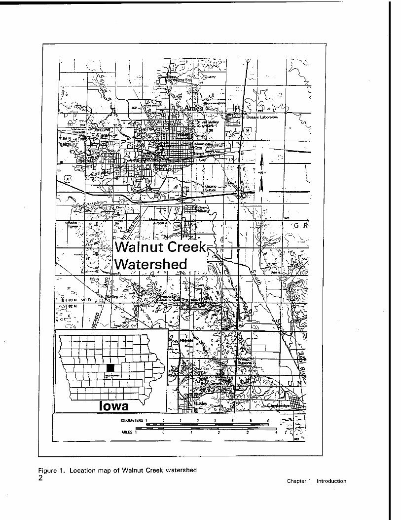
Figure 1. Location map of Walnut Creek watershed 2 Chapter 1 Introduction
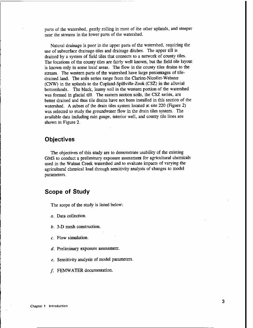
parts of the watershed, gently rolling in most of the other uplands, and steeper near the streams in the lower parts of the watershed.
Natural drainage is poor in the upper parts of the watershed, requiring the use of subsurface drainage tiles and drainage ditches. The upper till is drained by a system of field tiles that connects to a network of county tiles. The locations of the county tiles are fairly well known, but the field tile layout is known only in some local areas. The flow in the county tiles drains to the stream. The western parts of the watershed have large percentages of tile- drained land. The soils series range from the Clarion-Nicollet-Webster (CNW) in the uplands to the Copland-Spillville-Zook (CSZ) in the alluvial bottomlands. The black, loamy soil in the western portion of the watershed was formed in glacial till. The eastern section soils, the CSZ series, are better drained and thus tile drains have not been installed in this section of the watershed. A subset of the drain tiles system located at site 220 (Figure 2) was selected to study the groundwater flow in the drain tiles system. The available data including rain gauge, interior well, and county tile lines are shown in Figure 2.
Objectives
The objectives of this study are to demonstrate usability of the existing GMS to conduct a preliminary exposure assessment for agricultural chemicals used in the Walnut Creek watershed and to evaluate impacts of varying the agricultural chemical load through sensitivity analysis of changes to model parameters.
Scope of Study
The scope of the study is listed below:
a. Data collection.
b. 3-D mesh construction.
c. Flow simulation.
d. Preliminary exposure assessment.
e. Sensitivity analysis of model parameters.
/. FEMWATER documentation.
Chapter 1 Introduction

0) SZ CO
CO
2
03
u D
CO
D. CD
E
'5 > (0
co Q
3
Chapter 1 Introduction
2 Data Collection
Digital Elevation Data
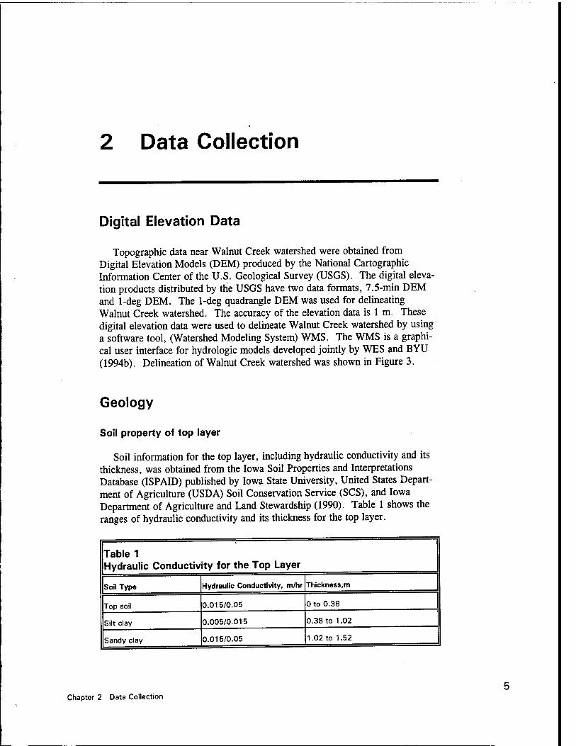
Topographic data near Walnut Creek watershed were obtained from Digital Elevation Models (DEM) produced by the National Cartographic Information Center of the U.S. Geological Survey (USGS). The digital eleva- tion products distributed by the USGS have two data formats, 7.5-min DEM and 1-deg DEM. The 1-deg quadrangle DEM was used for delineating Walnut Creek watershed. The accuracy of the elevation data is 1 m. These digital elevation data were used to delineate Walnut Creek watershed by using a software tool, (Watershed Modeling System) WMS. The WMS is a graphi- cal user interface for hydrologic models developed jointly by WES and BYU (1994b). Delineation of Walnut Creek watershed was shown in Figure 3.
Geology
Soil property of top layer
Soil information for the top layer, including hydraulic conductivity and its thickness, was obtained from the Iowa Soil Properties and Interpretations Database (ISPAID) published by Iowa State University, United States Depart- ment of Agriculture (USDA) Soil Conservation Service (SCS), and Iowa Department of Agriculture and Land Stewardship (1990). Table 1 shows the ranges of hydraulic conductivity and its thickness for the top layer.
Table 1 Hydraulic Conductivity for the Top Layer
Soil Type
Top soil
Silt clay
Sandy clay
Hydraulic Conductivity, m/hr Thickness.m
0.015/0.05
0.005/0.015
0.015/0.05
0 to 0.38
0.38 to 1.02
1.02 to 1.52
Chapter 2 Data Collection
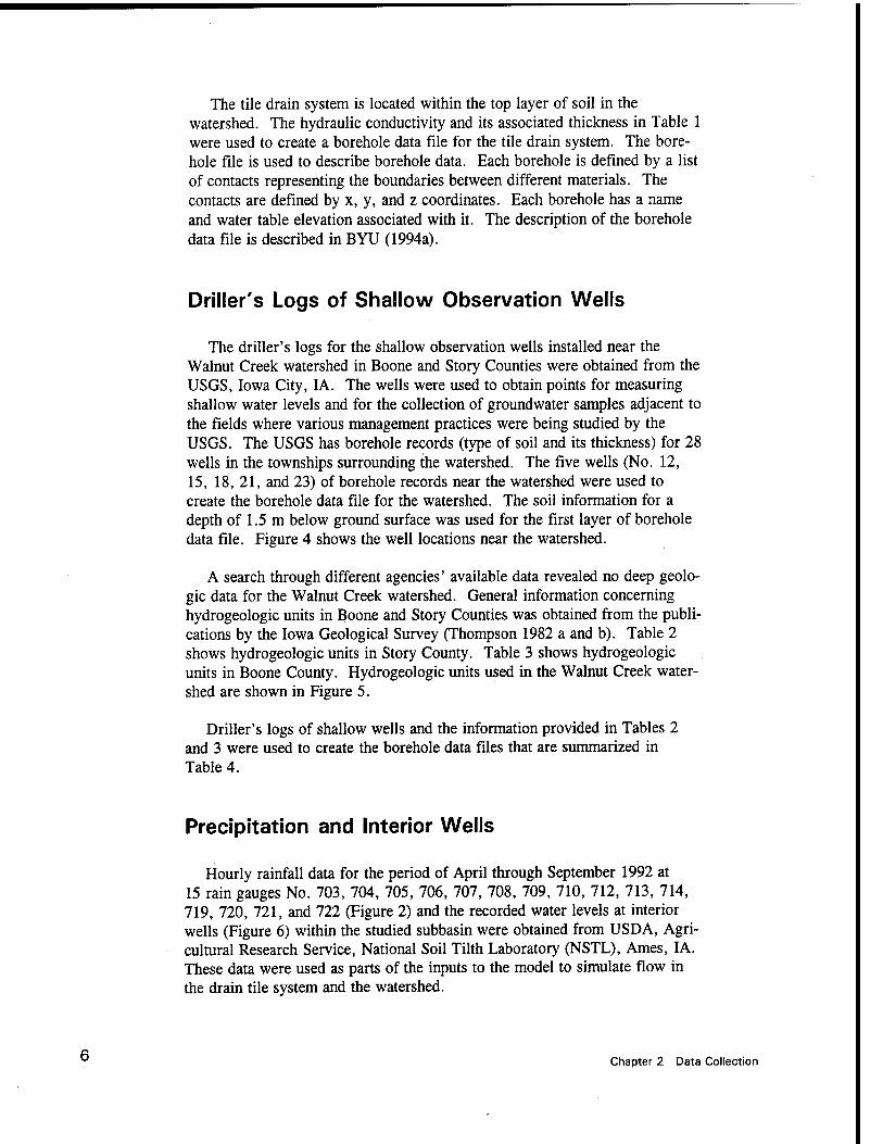
The tile drain system is located within the top layer of soil in the watershed. The hydraulic conductivity and its associated thickness in Table 1 were used to create a borehole data file for the tile drain system. The bore- hole file is used to describe borehole data. Each borehole is defined by a list of contacts representing the boundaries between different materials. The contacts are defined by x, y, and z coordinates. Each borehole has a name and water table elevation associated with it. The description of the borehole data file is described in BYU (1994a).
Driller's Logs of Shallow Observation Wells
The driller's logs for the shallow observation wells installed near the Walnut Creek watershed in Boone and Story Counties were obtained from the USGS, Iowa City, IA. The wells were used to obtain points for measuring shallow water levels and for the collection of groundwater samples adjacent to the fields where various management practices were being studied by the USGS. The USGS has borehole records (type of soil and its thickness) for 28 wells in the townships surrounding the watershed. The five wells (No. 12, 15, 18, 21, and 23) of borehole records near the watershed were used to create the borehole data file for the watershed. The soil information for a depth of 1.5 m below ground surface was used for the first layer of borehole data file. Figure 4 shows the well locations near the watershed.
A search through different agencies' available data revealed no deep geolo- gic data for the Walnut Creek watershed. General information concerning hydrogeologic units in Boone and Story Counties was obtained from the publi- cations by the Iowa Geological Survey (Thompson 1982 a and b). Table 2 shows hydrogeologic units in Story County. Table 3 shows hydrogeologic units in Boone County. Hydrogeologic units used in the Walnut Creek water- shed are shown in Figure 5.
Driller's logs of shallow wells and the information provided in Tables 2 and 3 were used to create the borehole data files that are summarized in Table 4.
Precipitation and Interior Wells
Hourly rainfall data for the period of April through September 1992 at 15 rain gauges No. 703, 704, 705, 706, 707, 708, 709, 710, 712, 713, 714, 719, 720, 721, and 722 (Figure 2) and the recorded water levels at interior wells (Figure 6) within the studied subbasin were obtained from USDA, Agri- cultural Research Service, National Soil Tilth Laboratory (NSTL), Ames, IA. These data were used as parts of the inputs to the model to simulate flow in the drain tile system and the watershed.
Chapter 2 Data Collection
o Q
> r!——co5b\>o:o~— \o
T3
0) 05
U 3
c o (D 0) c
"53 Q
00 0)
Chapter 2 Data Collection
T3 03 sz in L- 03 *-* 03
03 03
o +-»
C
03 03 C
CO T3 ^ O O 03
_03
O
o ■0
CD
Chapter 2 Data Collection
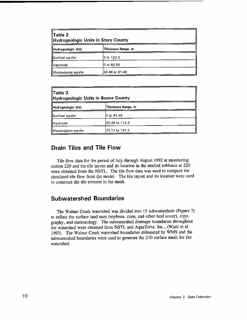
Table 2 Hydrogeologie Units in Story County
Hydrogeologie Unit Thickness Range, m
Surficial aquifer Oto 122.0
Aquiclude 0 to 65.55
Mississippian aquifer 30.48 to 91.46
Table 3 Hydrogeologie Units in Boone County
Hydrogeologie Unit Thickness Range, m
Surficial aquifer Oto 91.46
Aquiclude 30.48 to 114.3
Mississippian aquifer 73.17 to 137.2
Drain Tiles and Tile Flow
Tile flow data for the period of July through August 1992 at monitoring station 220 and the tile layout and its location in the studied subbasin at 220 were obtained from the NSTL. The tile flow data was used to compare the simulated tile flow from the model. The tile layout and its location were used to construct the tile element in the mesh.
Subwatershed Boundaries
The Walnut Creek watershed was divided into 15 subwatersheds (Figure 7) to reflect the surface land uses (soybean, corn, and other land cover), topo- graphy, and meteorology. The subwatershed drainage boundaries throughout the watershed were obtained from NSTL and AquaTerra, Inc., (Ward et al. 1993). The Walnut Creek watershed boundaries delineated by WMS and the subwatershed boundaries were used to generate the 2-D surface mesh for the watershed.
10 Chapter 2 Data Collection
■o
03
CO
-^ 03 03
u
C
-a 03 CO 3
CD
_03
O
O JD
o
CD
'> 03
15 O
to 03
Ü3
Chapter 2 Data Collection 11
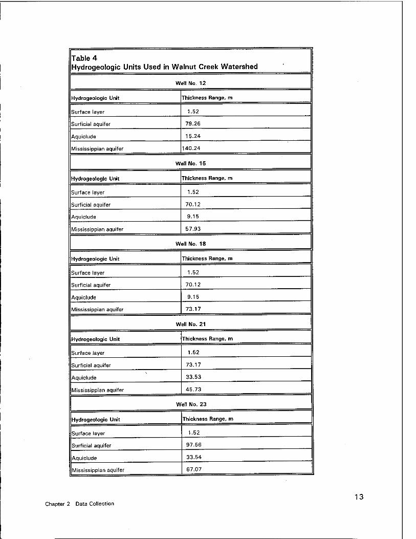
Table 4 Hydrogeologie Units Used in Walnut Creek Watershed
Well No. 12
Hydrogeologie Unit Thickness Range, m
Surface layer 1.52
Surficial aquifer 79.26
Aquiclude 15.24
Mississippian aquifer 140.24
Well No. 15
Hydrogeologie Unit Thickness Range, m
Surface layer 1.52
Surficial aquifer 70.12
Aquiclude 9.15
Mississippian aquifer 57.93
Well No. 18
Hydrogeologie Unit Thickness Range, m
Surface layer 1.52
Surficial aquifer 70.12
Aquiclude 9.15
Mississippian aquifer 73.17
Well No. 21
Hydrogeologie Unit Thickness Range, m
Surface layer 1.52
Surficial aquifer 73.17
Aquiclude 33.53
Mississippian aquifer 45.73
Well No. 23
Hydrogeologie Unit Thickness Range, m
Surface layer 1.52
Surficial aquifer 97.56
Aquiclude 33.54
Mississippian aquifer 67.07
Chapter 2 Data Collection 13
"ö5
c o CO Ü o
CD 0)
D3
14 Chapter 2 Data Collection
ü c
0 cd *ä —' CO £
< h-
LLI o CO CD
^ CO c o
^ "cd 0 z 0 0) v_ x: o ■4—•
b
ZJ o
C 03 0) i— cd
c 3 O
CD
T3 CD
SZ CO
CD
i
=3 C/3
s
Slj
J5 E
CD
CO
CD CD k_
O
C
CO CD
*i_ CO
T3 C D O J3
TJ CD .C
CO w CD ■*-»
CD
.n 3
CD
LL
Chapter 2 Data Collection 15
3 3-D Mesh Construction
16
2-D Surface Mesh
In order to generate a 3-D mesh, a 2-D surface mesh has to be generated first. Two 2-D surface meshes were generated by GMS. One mesh is repre- sented for a subdrain tile (inset mesh) system. The other is for the Walnut Creek watershed. The procedure for generating a 2-D mesh is described in BYU (1994a).
2-D surface mesh of the inset mesh
A 2-D surface mesh (Figure 8) for the drain tile system located at site 220 was generated, based on the layout and location of the drain tiles. The pur- pose of this mesh was to allow assignment of high hydraulic conductivity values in the drain tile elements to simulate the flow in the drain tile system.
2-D surface mesh of Walnut Creek watershed
The 2-D surface mesh (Figure 9) for the Walnut Creek watershed was generated based on the Walnut Creek watershed boundary delineated by WMS and 15 subwatershed boundaries (Figure 7). Each sub watershed contains many triangle elements. These triangle elements were generated by GMS using digital elevations data. This mesh allowed sensitivity analysis as to changes of land use or crop types, which reflect a different agricultural chemi- cal loading.
3-D Mesh
Two 3-D meshes of Walnut Creek watershed were created by GMS. One 3-D mesh was an inset mesh of the subdrain tile system of the watershed. This mesh was used to test and evaluate schemes to represent the drain tile feature of the watershed. The other 3-D mesh was used to represent the entire watershed based on the best available data. These meshes were used as the
Chapter 3 3-D Mesh Construction
JC CO CD
E +-> CD CO C
c CD
E CD
03 O CO
CD c o 'en c CD
E
6 5
oo CD
3 C5)
Chapter 3 3-D Mesh Construction 17
03 XT CO 1_
CD +-» CD
§ CD CD i_
U 3 C
C CD
E _CD CD
CD Ü CO H— 1_
3 co
"c5 c o CO c CD
E i o
r-
O) CD i_
D) Li-
Chapter 3 3-D Mesh Construction 19
input of the geometry file to the FEMWATER model for studying the movement of agricultural chemicals applied to the surface. The procedure for generating a 3-D mesh is described in BYU (1994a).
Mesh no.1 - inset mesh
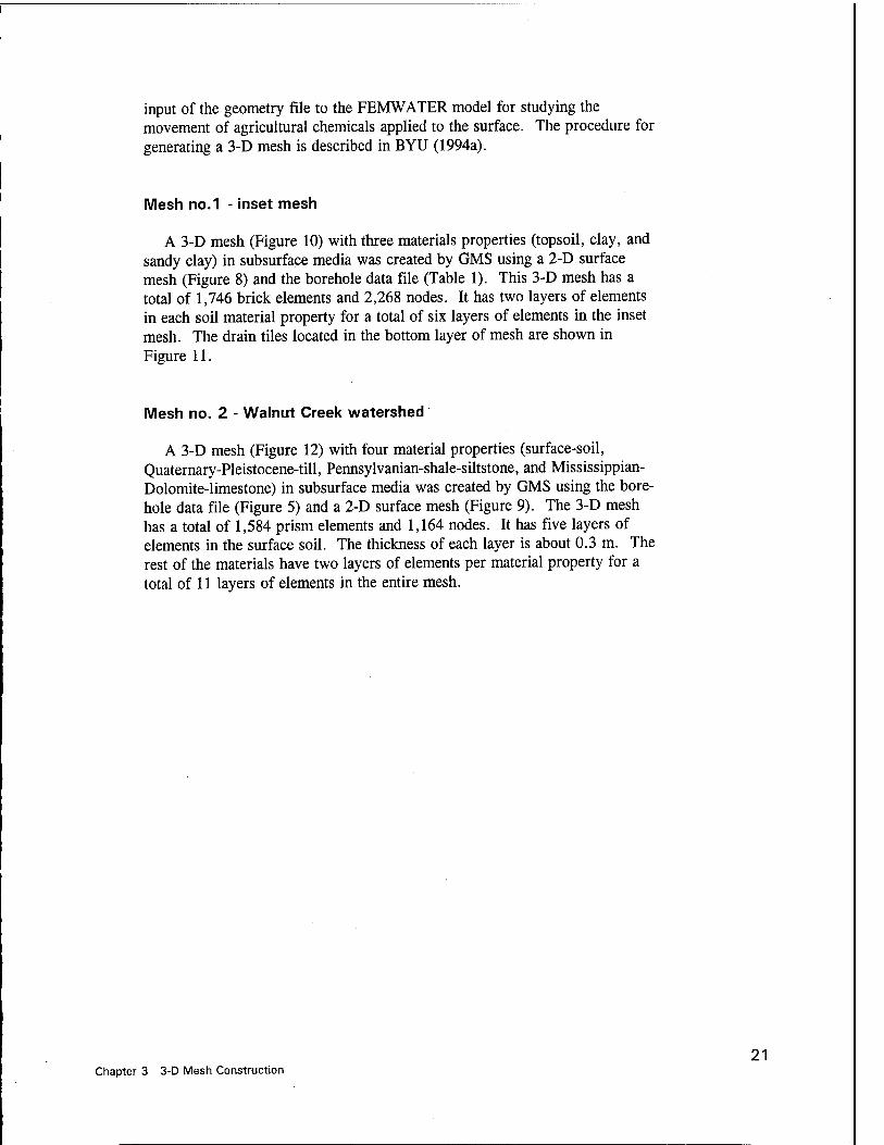
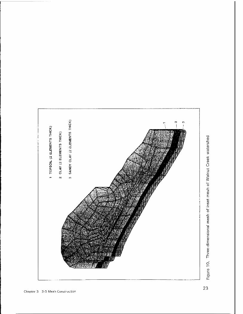
A 3-D mesh (Figure 10) with three materials properties (topsoil, clay, and sandy clay) in subsurface media was created by GMS using a 2-D surface mesh (Figure 8) and the borehole data file (Table 1). This 3-D mesh has a total of 1,746 brick elements and 2,268 nodes. It has two layers of elements in each soil material property for a total of six layers of elements in the inset mesh. The drain tiles located in the bottom layer of mesh are shown in Figure 11.
Mesh no. 2 - Walnut Creek watershed
A 3-D mesh (Figure 12) with four material properties (surface-soil, Quaternary-Pleistocene-till, Pennsylvanian-shale-siltstone, and Mississippian- Dolomite-limestone) in subsurface media was created by GMS using the bore- hole data file (Figure 5) and a 2-D surface mesh (Figure 9). The 3-D mesh has a total of 1,584 prism elements and 1,164 nodes. It has five layers of elements in the surface soil. The thickness of each layer is about 0.3 m. The rest of the materials have two layers of elements per material property for a total of 11 layers of elements in the entire mesh.
21 Chapter 3 3-D Mesh Construction
* _ <N CO O i
ü I 1- co 1—
ä^
I \ 1 /
1 //I-.; JAf z 111 /^vyfe?'v'iffen>v.^ji«vÄM^K/ 2 111 m cg X':; •:£W'*™*-'V.: -iyMm$y UJ
CM
_J i /SJ-f/M o CO a. O
<
SA
ND
Y ■1
yT'^^^^-i'A^aSI^^^ÄS^
X^^^^^^m /^^^^ßm
/fe''^^*T.^ÄSßs^i3rafiil^^Ä^ $%ä3sss£J$S*^ H?aBSSr
'i i lii f 'n ' i irtiihi1 iMwr *E * m ii ^i "JiwWil iW i MWi rfi ' r
t£f$ «HC^pSn^inr R:i r^^^S^^^^P^^WMJM^aB^S'
*i^^^¥iaP^^Sffflfe'A;*"ÄlP^ EFn
WmMS3m0Mf
^^^^MBW
x: C/3 1_ 0
■»-» ca
CD CD
o 3 C
x: CD
CD tn c
x: CD
E "CD c o
c CD
E
CD CD
x: r-
D5
Chapter 3 3-D Mesh Construction 23
sz to 03
E ■*-»
03 C/3 C
E o o
JD
03 JZ
c o 03 Ü O
Q
D3
Chapter 3 3-D Mesh Construction 25
-*: u
J: 2 o
o 'E c CM " *
'£ >f> a> \ \ 0) c
0) E \
ff K9 ^ c 0)
E E 0
CM £|V)\<JMH| ^BA^H ^BL CD '— feädöJIBM KvH H&
0) CM a) c ^^pH wk -* CM (U o
o ' C To !E — o CD
(0 ~ U3 E JMfl^^PP BL
c CD c 05 i /ffiT*Ma%^J%&lr^B H& a (I) +J /'i Tfc^ ■r*^'W\*-3^E^^H ^Dz
E o .3! E Z-£,'l. ./£»-*'*£-] (D o CO o X* r'*A'ß']Blv'*tu WJ 'Si/cS^H mWi r;
c (I)
IT) 'o> o a Wlmni^m\ mmnmmm
"5 0)
a. CD
c c re 'a ÄHS W%m W CO > a llJSfaSÄIwffllj^MRgMP i C >. 'm ~-a^nJH&*$nt*ui fai&mm mwMBIi o
3 re 3
(0 c c a>
in 'in in
m w W a 0. 2 Bf fif T?nifit' IM |Mf^
CM n "3-
M
WKBn w Kffl IH ■ III II I
flffii 'Xfbjtn füi «BfiSS ||p| HÜ IH ÜH WMMffi ITOIOM HHffl
Isis lÜ «KM*
&:&'. |1|§ BraäM HHHB fjfraß«
m ^H
Hü sü23^l ^H 'r'l^&'lA
M s [»St Brawl llll BftlfiP IESSI BDHR HlS
£J5 I Um III ü l^^ii P |m^ W/m W W^^fm «*** jSgfljl!
wMffljiM w mWU\ Ma n ■/l ■
|U m Wlm\ m 1 WmW
mWI Amt mm
^^BKS
•o CD
_C c/j
CD
Cö
CD CD
U
C/3 CD
e 15 c
_o 'c/i c CD
E
CD CD
x: H
Chapter 3 3-D Mesh Construction 27
4 Flow Simulation
Groundwater flow was simulated by the FEMWATER model. The inputs to the model consist of a geometry file; a combined boundary conditions (BC) file of model parameters, boundary conditions, and initial conditions; and a super file. These files are typically created by GMS during the preprocessing stages.
These files use a character-style input and can be entered in free-field format. The geometry file contains the data describing nodes and elements. The BC files contain data describing boundary conditions, initial conditions, material properties, and model parameters that control analysis. The super file contains the names of input files and output files.
The geometry file is a data file that contains the information of a 3-D mesh (including element connecting table and nodal point coordinates). Each line of the geometry file is preceded by a two- or three- letter code specifying the type of data contained on the line. The first input line has a label (3DFEMGEO) that helps to identify the data on the line. Tl-3 cards are the title cards. A GE card contains the element information. GE cards define element and material associated with the element. Two types of 3-D element (brick and prism) are supported by the model. The eight node brick elements can be used for flow simulation only. The six node prism elements can be used for flow and transport simulations. A GN card contains nodal point information. GN cards define the nodal point location. The END card signi- fies the end of the geometry file.
The FEMWATER model requires many input data. These data include fluid properties, analysis parameters, and material properties. The input data are divided into eight groups: titles, run option parameters, iteration parameters, time control parameters, control tracking parameters, material properties, fluid properties, and soil properties for the unsaturated zone.
Three title cards are used for users to specify title and detailed information for the study. The run option parameters are used to select the type of simu- lation such as steady state or transient, flow or transport, and flow and trans- port combined. The iteration parameters are used to specify iteration numbers allowed for solving the coupled nonlinear equations for flow and transport. The time control parameters are used to specify simulation time and
Chapter 4 Flow Simulation 29
computational time-step. The output control parameters are used to specify the printed options and output control for post-processing. The control tracking parameters are used to specify the tracking scheme. The material property parameters are used to specify hydraulic conductivity or permeability of the material. The soil property parameters are used to specify the soil characteristics curves for the unsaturated zone.
The boundary segment can be used as one of five types of boundary conditions:
a. Dirichlet (total head).
b. Neumann (gradient flux).
c. Cauchy (total flux).
d. Variable (rainfall-seepage) boundary.
e. Point (well) source/sink boundary conditions.
The initial conditions for the flow and transport simulations can either be obtained by solving steady-state solution or by defining through the field measurements.
The FEMWATER super file is a special type of file used by the GMS to organize the individual files for input to the FEMWATER and the GMS. The super file is a text file that contains the names of the input files and output files.
The detailed descriptions of the model's inputs are described in User's Manual (Lin and Yeh 1995). The procedure for generating the input data to the FEMWATER model is described in BYU (1994a).
Simulated Flow for Inset Mesh
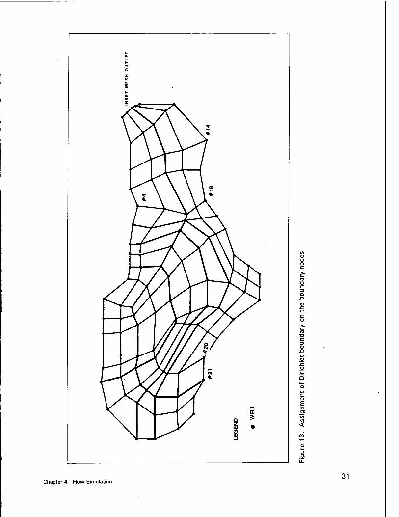
The boundary of the region is bounded by fresh water. No flux was imposed on the bottom of the region. The pressure head is assumed to be hydrostatic. Rainfall as flux was imposed on the top surface elements of the region The Dirichlet boundary condition was assumed at the boundaries. The water levels of observation wells at No. 21, 20, 18, 14, and 4 were used as the Dirichlet boundary along the boundary nodes (Figure 13). The water levels at the rest of the nodes along the boundary were estimated and inter- preted by the observation wells near the studied area (Figure 3). Table 5 shows the water levels at the observed wells.
30 Chapter 4 Flow Simulation
co
"O o c
to T3 C
O Si
CD J= +-»
C o
CD
c 3 O
X)
c CD
E c ro
'co CO
< CO
3
Chapter 4 Flow Simulation 31
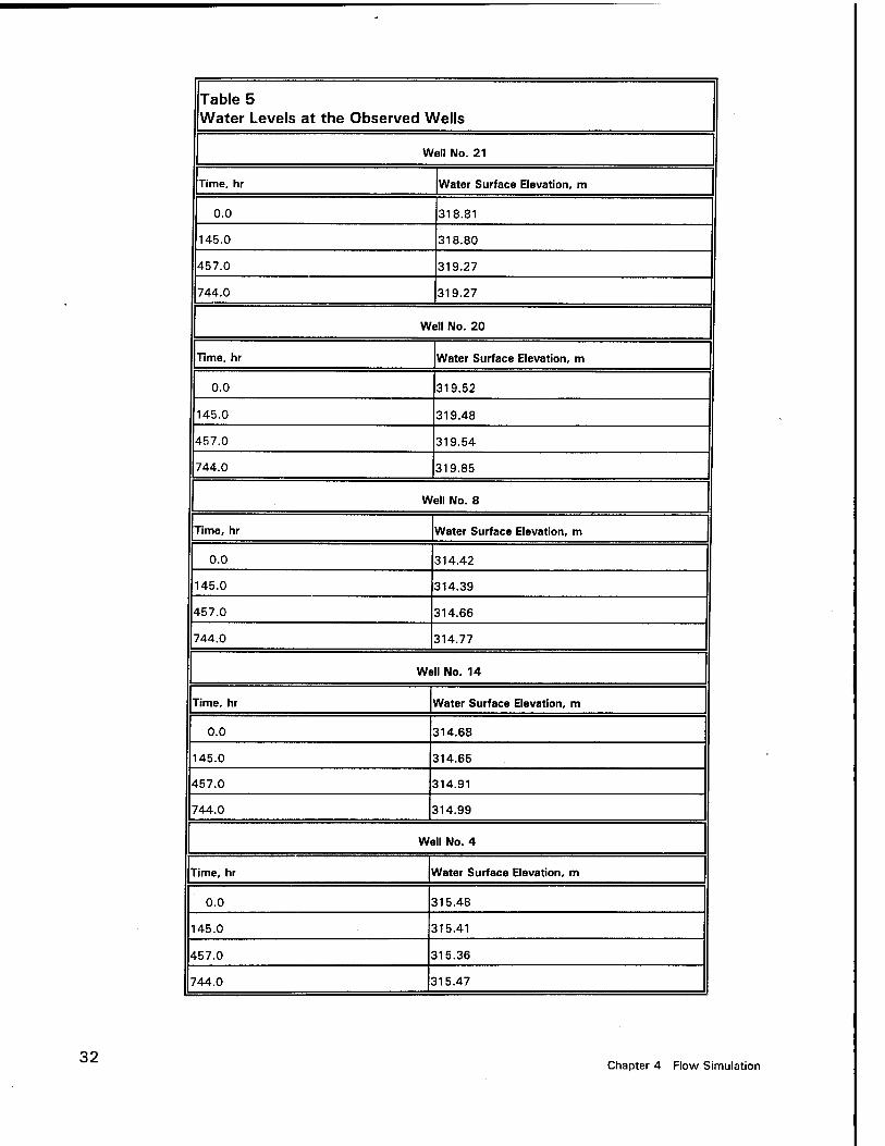
Table 5 Water Levels at the Observed Wells
Well No. 21
Time, hr Water Surface Elevation, m
0.0 318.81
145.0 318.80
457.0 319.27
744.0 319.27
Well No. 20
Time, hr Water Surface Elevation, m
0.0 319.52
145.0 319.48
457.0 319.54
744.0 319.85
Well No. 8
Time, hr Water Surface Elevation, m
0.0 314.42
145.0 314.39
457.0 314.66
744.0 314.77
Well No. 14
Time, hr Water Surface Elevation, m
0.0 314.68
145.0 314.65
457.0 314.91
744.0 314.99
Well No. 4
Time, hr Water Surface Elevation, m
0.0 315.48
145.0 315.41
457.0 315.36
744.0 315.47
32 Chapter 4 Flow Simulation
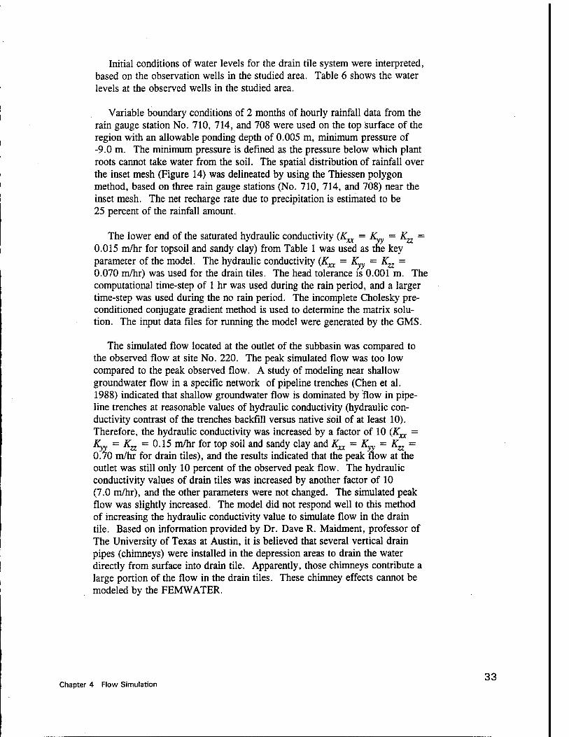
Initial conditions of water levels for the drain tile system were interpreted, based on the observation wells in the studied area. Table 6 shows the water levels at the observed wells in the studied area.
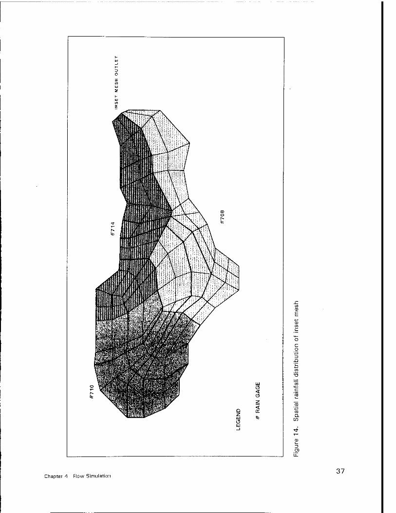
Variable boundary conditions of 2 months of hourly rainfall data from the rain gauge station No. 710, 714, and 708 were used on the top surface of the region with an allowable ponding depth of 0.005 m, minimum pressure of -9.0 m. The minimum pressure is defined as the pressure below which plant roots cannot take water from the soil. The spatial distribution of rainfall over the inset mesh (Figure 14) was delineated by using the Thiessen polygon method, based on three rain gauge stations (No. 710, 714, and 708) near the inset mesh. The net recharge rate due to precipitation is estimated to be 25 percent of the rainfall amount.
The lower end of the saturated hydraulic conductivity (K^ = ÄL, = Kzz = 0.015 m/hr for topsoil and sandy clay) from Table 1 was used as the key parameter of the model. The hydraulic conductivity (K^ = R' = K^ = 0.070 m/hr) was used for the drain tiles. The head tolerance is 0.001 m. The computational time-step of 1 hr was used during the rain period, and a larger time-step was used during the no rain period. The incomplete Cholesky pre- conditioned conjugate gradient method is used to determine the matrix solu- tion. The input data files for running the model were generated by the GMS.
The simulated flow located at the outlet of the subbasin was compared to the observed flow at site No. 220. The peak simulated flow was too low compared to the peak observed flow. A study of modeling near shallow groundwater flow in a specific network of pipeline trenches (Chen et al. 1988) indicated that shallow groundwater flow is dominated by flow in pipe- line trenches at reasonable values of hydraulic conductivity (hydraulic con- ductivity contrast of the trenches backfill versus native soil of at least 10). Therefore, the hydraulic conductivity was increased by a factor of 10 (K^ = Kyy — Ku = 0.15 m/hr for top soil and sandy clay and K^ = ÄL, = Ka = 0.70 m/hr for drain tiles), and the results indicated that the peak flow at the outlet was still only 10 percent of the observed peak flow. The hydraulic conductivity values of drain tiles was increased by another factor of 10 (7.0 m/hr), and the other parameters were not changed. The simulated peak flow was slightly increased. The model did not respond well to this method of increasing the hydraulic conductivity value to simulate flow in the drain tile. Based on information provided by Dr. Dave R. Maidment, professor of The University of Texas at Austin, it is believed that several vertical drain pipes (chimneys) were installed in the depression areas to drain the water directly from surface into drain tile. Apparently, those chimneys contribute a large portion of the flow in the drain tiles. These chimney effects cannot be modeled by the FEMWATER.
Chapter 4 Flow Simulation 33
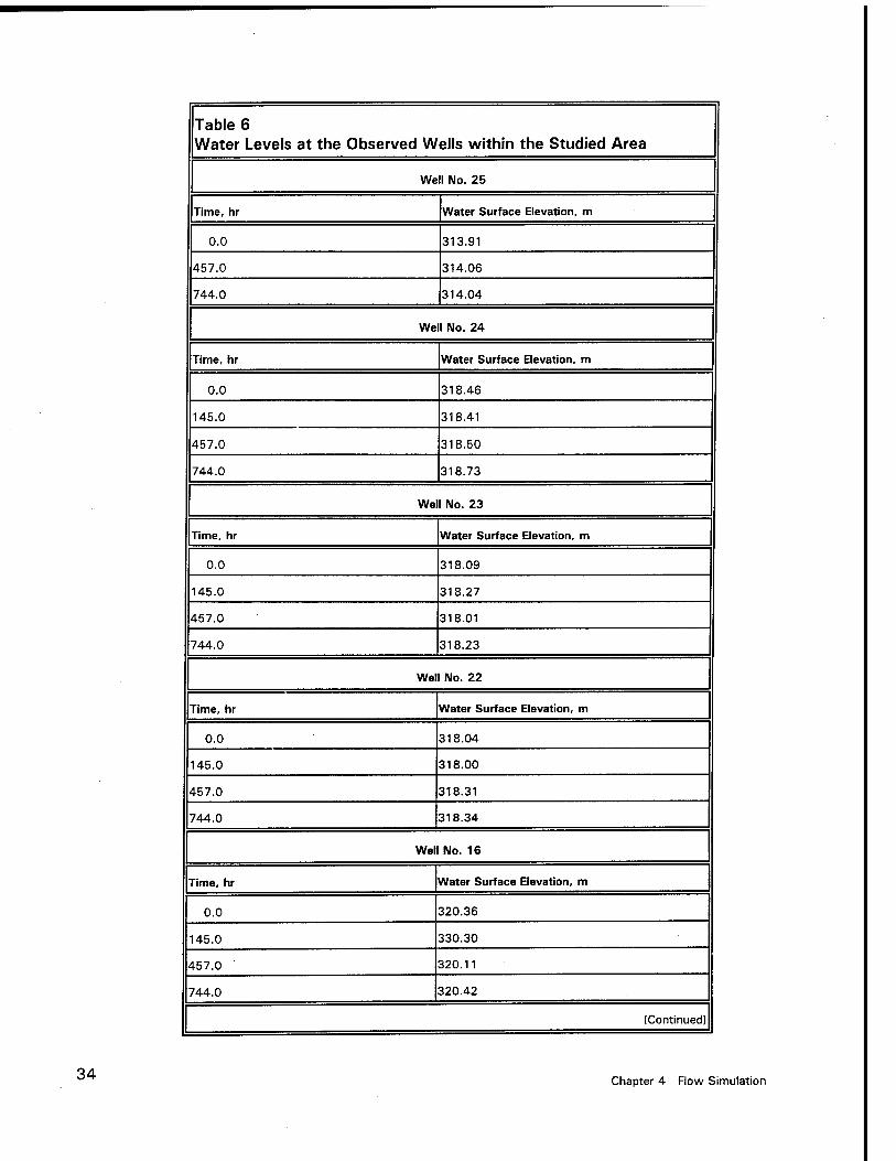
Table 6 Water Levels at the Observed Wells within the Studied Area
Well No. 25
Time, hr Water Surface Elevation, m
0.0 313.91
457.0 314.06
744.0 314.04
Well No. 24
Time, hr Water Surface Elevation, m
0.0 318.46
145.0 318.41
457.0 318.50
744.0 318.73
Well No. 23
Time, hr Water Surface Elevation, m
0.0 318.09
145.0 318.27
457.0 318.01
744.0 318.23
Well No. 22
Time, hr Water Surface Elevation, m
0.0 318.04
145.0 318.00
457.0 318.31
744.0 318.34
Well No. 16
Time, hr Water Surface Elevation, m
0.0 320.36
145.0 330.30
457.0 320.11
744.0 320.42
(Continued)
34 Chapter 4 Flow Simulation
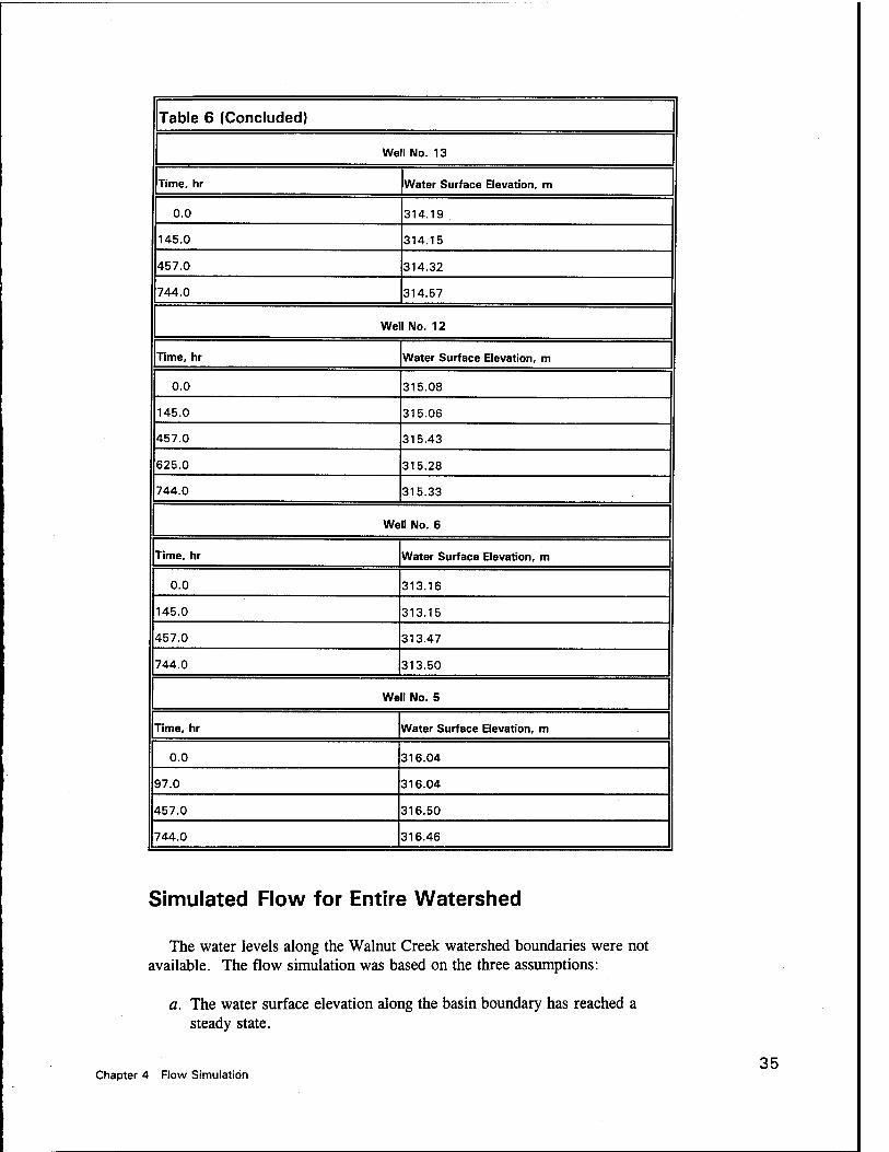
Table 6 (Concluded)
35
Well No. 13
Time, hr Water Surface Elevation, m
0.0 314.19
145.0 314.15
457.0 314.32
744.0 314.57
Well No. 12
Time, hr Water Surface Elevation, m
0.0 315.08
145.0 315.06
457.0 315.43
625.0 315.28
744.0 315.33
Well No. 6
Time, hr Water Surface Elevation, m
0.0 313.16
145.0 313.15
457.0 313.47
744.0 313.50
Well No. 5
Time, hr Water Surface Elevation, m
0.0 316.04
97.0 316.04
457.0 316.50
744.0 316.46
Simulated Flow for Entire Watershed
The water levels along the Walnut Creek watershed boundaries were not available. The flow simulation was based on the three assumptions:
a. The water surface elevation along the basin boundary has reached a steady state.
Chapter 4 Flow Simulation
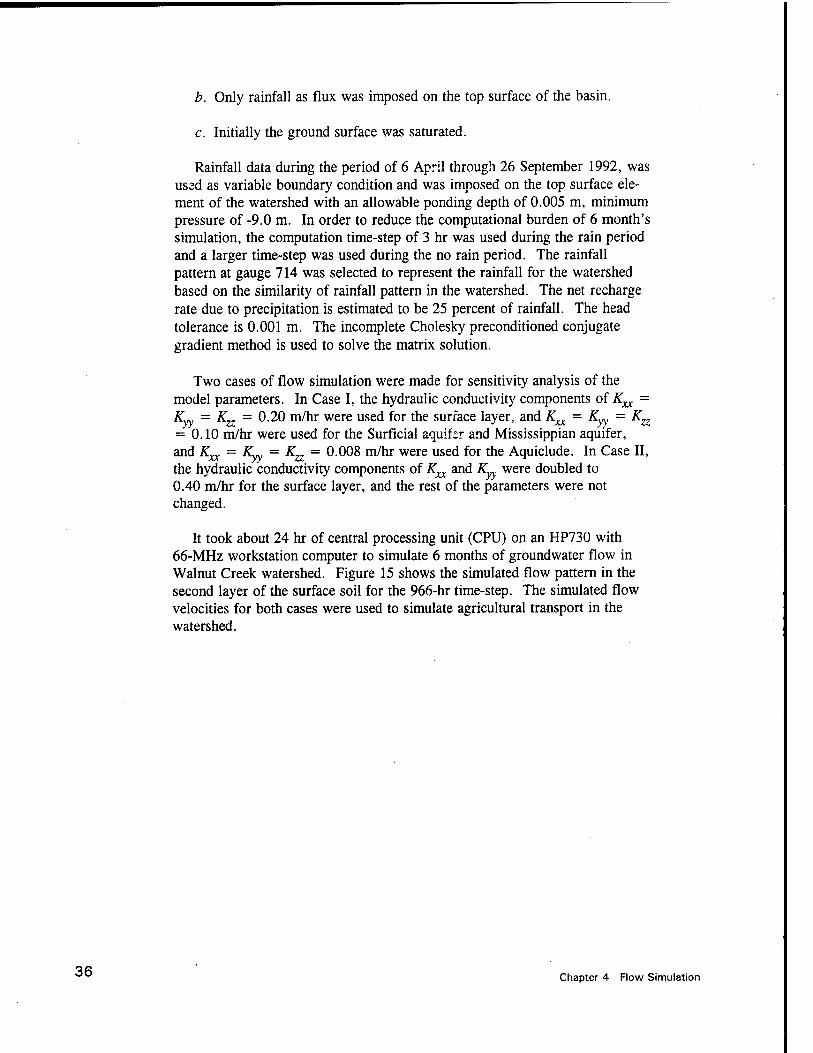
b. Only rainfall as flux was imposed on the top surface of the basin.
c. Initially the ground surface was saturated.
Rainfall data during the period of 6 April through 26 September 1992, was used as variable boundary condition and was imposed on the top surface ele- ment of the watershed with an allowable ponding depth of 0.005 m, minimum pressure of -9.0 m. In order to reduce the computational burden of 6 month's simulation, the computation time-step of 3 hr was used during the rain period and a larger time-step was used during the no rain period. The rainfall pattern at gauge 714 was selected to represent the rainfall for the watershed based on the similarity of rainfall pattern in the watershed. The net recharge rate due to precipitation is estimated to be 25 percent of rainfall. The head tolerance is 0.001 m. The incomplete Cholesky preconditioned conjugate gradient method is used to solve the matrix solution.
Two cases of flow simulation were made for sensitivity analysis of the model parameters. In Case I, the hydraulic conductivity components of K^ = Kyy = K^ = 0.20 m/hr were used for the surface layer, and K^ = Ky = K^ = 0.10 m/hr were used for the Surficial aquifer and Mississippian aquifer, and Kxx - K^ = K7Z = 0.008 m/hr were used for the Aquiclude. In Case II, the hydraulic conductivity components of K^ and K were doubled to 0.40 m/hr for the surface layer, and the rest of the parameters were not changed.
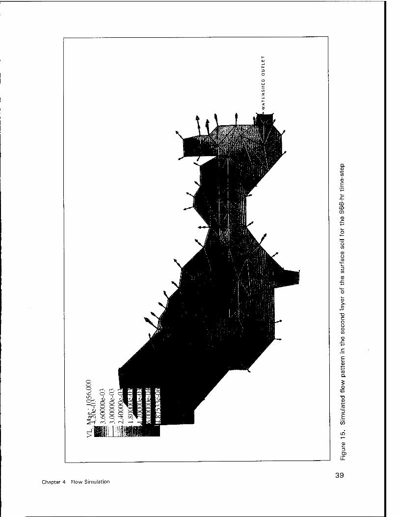
It took about 24 hr of central processing unit (CPU) on an HP730 with 66-MHz workstation computer to simulate 6 months of groundwater flow in Walnut Creek watershed. Figure 15 shows the simulated flow pattern in the second layer of the surface soil for the 966-hr time-step. The simulated flow velocities for both cases were used to simulate agricultural transport in the watershed.
36 Chapter 4 Flow Simulation
en CD
CD
c
c o 3
Ü3
XI
"TO 4— c
'co
en a.
CD
CD
Chapter 4 Flow Simulation 37
03
<n i
03
E
CO CD <J)
03
o c/3
03 O CD
M— I»
tn
0)
03 > JS ■D c o o 03
03
C
03
CD a
T3 03 4-* _CD
E CO
03
LL
Chapter 4 Flow Simulation 39
5 Preliminary Exposure Assessment
General Description
The preliminary exposure assessment utilized available data to simulate actual field conditions within the Walnut Creek watershed so that the effects of the current land use practices and agrichemical applications on groundwater quality could be determined. Typical use of the herbicide atrazine in the watershed corresponded to a pre-emergence application to acreage planted with corn. This type of application of the herbicide atrazine was incorporated into the simulation. The primary objective of the preliminary exposure assess- ment in the Walnut Creek watershed was to demonstrate the usability of the GMS through application of the FEMWATER model. The simulated flow velocity discussed in Chapter 4 was used to simulate agricultural transport in the watershed. The FEMWATER model allows for the evaluation of the impact of the application of agrichemicals on groundwater quality.
Corn and soybeans are the primary production crops within the Walnut Creek watershed. Approximately 88 percent of the watershed is represented by one of these two land uses (Donigian et al. 1993). Farming practices within the watershed utilize a corn-soybean rotation scheme. The other 12 percent of the watershed contains scattered pastures,wetland forests along stream channels, residential areas, and road networks. The primary area of interest for the preliminary exposure assessment is the acreage planted in corn. Figure 16 shows the areas within the watershed that were planted in corn for the 1992 growing season. The total amount of acreage in corn was approximately 2,500 ha.
Parameter Development
Data Availability
The Walnut Creek watershed has been extensively monitored as part of the EPA (MASTER) Midwest Agricultural Surface/Subsurface Transport and Effects Research program. The Walnut Creek watershed was one of five
Chapter 5 Preliminary Exposure Assessment 41
42
selected Management Systems Evaluation Areas (MSEA) which are located throughout the Midwest. The MASTER program was developed as part of the USDA and the USGS research program developed in response to the President's Water Quality Initiative which emphasizes the interactions of agricultural practices and their effects on both surface and groundwater quality. Participants of the Walnut Creek MSEA include the EPA laboratories in Athens, GA; Las Vegas, NV; Duluth, MN; Corvallis, OR; and Ada, OK; USGS; and USDA National Soil Tilth Laboratory (NSTL) in Ames, IA. The NSTL was responsible for performing the field site monitoring on the Walnut Creek watershed.
The extensive monitoring of the Walnut Creek watershed has resulted in the development of a comprehensive database (Ward et al. 1993). At the time this study began, data were available through 1992. The present database includes information relating to climatology, soil physical properties, geology, agricultural production, tile drains, gauge stations, and water quality param- eters for surface and groundwater. Currently, only a small fraction of the total database is available for release. The time required for data quality con- trol measures and reduction techniques has limited the amount of data avail- able for this preliminary exposure assessment.
One limiting factor for the selection of a simulation period was the avail- ability of weather data. The collection of meteorological data from the Walnut Creek watershed did not begin until April 1991. Furthermore, the data collected in 1991 failed to include several precipitation stations in the eastern portion of the watershed. Based on data availability, it was decided to run the preliminary exposure assessment simulation for a period of 173 days in 1992. The simulation was started on 6 April (Julian day 97) and ended on (26 September) Julian day 270. Thus, only the 1992 growing season would be simulated.
Selected parameters
Atrazine was the selected agrichemical to be simulated in the transport simulation. In the Walnut Creek watershed, atrazine is typically applied with metolachlor to control both annual grass and broadleaf weeds in acreage planted with corn. A pre-emergence banded application is sprayed directly onto the crop row. Crop rows range in size from approximately 25 to 30 cm depending on the planter being used. Atrazine is the common name for 2-chloro-4(ethylamino)-6-(isopropylamino)-5,-triazine and is a triazine herbicide. Herbicides in the triazine family are not subject to excessive leaching from the soil and are reversibly adsorbed to clay and organic colloids (Klingman and Ashton 1982).
As previously mentioned, the selected simulation period was for the 1992 growing season. The amount of atrazine applied during this growing season was given by Donigian, Chinnaswamy, and Beyerlein (1993) to be 0.4 kg ha"1
of active ingredient. This value reflects 578 kg of active ingredient being
Chapter 5 Preliminary Exposure Assessment
c o e/3 CO 03 c/3
en c
CM CD CD
0) -C
o Ü
"a CD
■t-J C CD
CD a) co CD
o < CO
3 en
Chapter 5 Preliminary Exposure Assessment 43
applied to 1,413 ha of treated corn. The banded application of atrazine was made on 6 May (Julian day 127), and the corn was planted 4 days after this event. For the preliminary exposure assessment, the 0.4 kg ha"1 rate was utilized. Additionally, the entire 2,500 ha of corn rather than just the 1,413 ha will be treated at the 0.4 kg ha"1 rate. This allows for evaluation of the maximum possible amount of corn acreage treated with atrazine for the 1992 growing season.
The FEMWATER model allows for specific chemical and soil properties which effect the transport process to be entered. These properties included the distribution coefficient (Kd), decay constant (0), molecular diffusion coef- ficient (D*), longitudinal dispersion (a£), lateral (transverse) dispersion (aT), tortuosity (7), and bulk density (pB). The distribution coefficient describes the partitioning between the liquid and the solids. The coefficient provides a valid representation of the reaction between the liquid and solids given that this can be assumed to be linear and instantaneous. The effect of the distribution coef- ficient on mass transport is to reduce the amount of material available for transport through adsorption. Decay of the chemical also reduces the amount of chemical available for transport. As the decay constant increases the amount of available chemical decreases. Molecular diffusion is accounted for in the molecular diffusion coefficient. The process of molecular diffusion serves to spread the contaminant concentration profile in advance of the typi- cal breakthrough curve observed with no molecular diffusion or mechanical dispersion. The molecular diffusion coefficient is an important contributor only at low velocities. At high velocities, the spread in the contaminant con- centration profile is attributed to mechanical mixing. Mechanical mixing is a function of the velocity and the dispersion coefficients. Dispersion is typically stronger in the longitudinal direction of flow than the lateral one (Freeze and Cherry 1979). Velocity of water through the system is affected by physical properties of the soil including the tortuosity and the bulk density. Tortuosity quantifies the twists and turns along the flow path. The higher the value, the more twists and turns encountered and the net effect is a decrease in velocity along the flow path. The bulk density of the soil can further effect the veloc- ity. The higher the bulk density the greater the compaction of the soil. Therefore, soils with higher bulk densities have more pore volume occupied by solids and less with air. Thus, less pore space is available for flow through the soil. All of the above parameters effect contaminant transport through the soil profile.
Each of the parameters was assigned a value which most closely approxi- mated actual conditions in the Walnut Creek watershed during the selected simulation period. Parameters were set as follows:
a. The bulk density was set equal to 1200 kg/m3.
b. The tortuosity was set equal to 1.0 (dimensionless m/m).
c. The distribution coefficient was set to 10 L//kg.
Chapter 5 Preliminary Exposure Assessment 45
46
d. The decay constant was set equal to 4.8E-4/hr.
e. The applied load was 0.0033 ppt.
The molecular diffusion and longitudinal and lateral dispersion coefficients were assigned values of zero for this study. This was based on the dominant transport mechanism in the watershed being attributed to advection and lack of data to accurately select values for these parameters. Other physical parameters used for the simulation have been described in Chapter 4, which describes the flow simulation.
Simulation Results
The preliminary exposure assessment was conducted utilizing the selected parameters. Output generated from the FEMWATER simulation was graphi- cally displayed within the GMS. Options within the GMS allowed for the data to be viewed at any selected time-step, depth, and cross section and as a film loop. The film loop provided an incremental view of the change in the atrazine concentrations over time for any selected view of the watershed.
One important objective of the preliminary exposure assessment was to determine the depth to which the applied atrazine would migrate. This objective was accomplished by application of the film loop tool. The time series atrazine concentration data was viewed over time at selected soil depths. The soils in the watershed were divided into four material types. The first soil type encompassed the surface soil and contained five layers each approxi- mately 30.5 cm in depth. The three remaining soil types were divided into two layers each. The depth of the second, third, and fourth layers were 30 m, 15 m, and 20 m, respectively. Soil layers were checked incrementally downward for the presence of the herbicide. The analysis revealed that atrazine migrated only into the surface soil during the simulation period. The last soil layer found to contain atrazine was the fourth layer in the first soil material. This equated to a soil depth of approximately 1.2 m. No atrazine was found below this depth. The time at which the breakthrough occurred at this depth was 1056 hr into the simulation. At the end of the simulation, 4152 hr, no atrazine was detected in any of the soil layers.
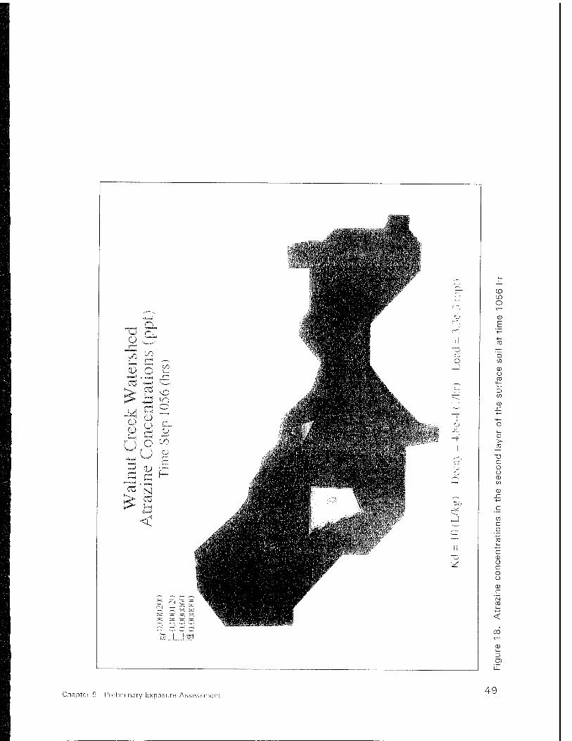
Figures 17 and 18, respectively, show the concentration of atrazine in the surface soil at the second layer for the 966-hr and 1056-hr time-steps. These figures show the locations within the watershed where atrazine leaches into the ground. The maximum concentration distribution occurred at the 1056-hr time-step. After this time-step, the concentration in the soil layer decreased rapidly. These figures further serve to demonstrate the output that can be obtained from the GMS. Hard copy output could be printed for any desired soil layer. The remaining soil layers that contained atrazine exhibited similar trends.
Chapter 5 Preliminary Exposure Assessment

d. ™Ö r-, a,) er CO C/j
CD O C\j +_j
r~'
cd ^-"
1^- £H
Cl'S
<D CJ 0_Ji
t-4 GO u o U
'—> cu 'CZ
C3 [v.
<
CLi_fiB
_1
II
bo
™4 c '—' o . cc
II ^ .,, L CD o ^ c
o o
CD CD CD
CD
E
o CO
CD O 03
CO
ID
cc
o o
<
en Li-
Chapter 5 Preliminary Exposure Assessment 47
rU FT 0) o~:
T? ^ ul C - a) o - Co +-> o
"> co ^
~f{ CD 5^ O c--'
O L^
g g tf
v.U
«1
Mm*.
Wi
15; ...LJJE!
CD LD O
rt O o tn
_j CD ü CO
M—
, , _J __ (/) —. CD ■"—■ _c —i- ■t—'
i M—
o O DC" \
CD >
|] CD
-^. X3 .-^ C O
O O /*—\ 0 1 , W
CD , _ JZ
bJj ■l-"
JjS C
_j c/3 c
r . o CD
ii -t-< <— -r} CD 'V Ü •—. C
o o CD C
N CO
<
CO
Chapter 5 Pn-liminary Exposure Assessment 49
Results from the simulation indicated that atrazine applied during the 1992 growing season did not migrate into the deep soil layers. Additionally, no atrazine could be detected at the end of the 173-day simulation. The highest concentration of atrazine was detected in the western section of the watershed due to the larger amount of corn acreage in this area.
Chapter 5 Preliminary Exposure Assessment 51
6 Sensitivity Analysis
Genera! Descrlp
A sensitivity analysis was conducted to gain an understanding of the effect of altering selected input parameters on the FEMWATER simulation output. Parameters that were varied included the acreage loaded with the atrazine (alternative land use), saturated hydraulic conductivity, distribution coefficient, decay constant, and loading rate. The majority of these parameters can be altered by running only the transport section of the FEMWATER code, thus avoiding the task of re-running the flow portion. The exception is hydraulic conductivity, which must be run utilizing the flow section of the code.
Analysis Protocol
The base conditions for the sensitivity analysis were those used for the preliminary exposure assessment that is described in Chapter 5. The base graphs used for comparison were Figures 17 and 18. Each of the previously mentioned parameters were changed individually and the effect on the simula- tion output was analyzed. The scales, time-steps, and locations within the watershed for each of the resulting graphs were the same for comparison and evaluation purposes. Actual maximum and minimum values for each of the parameters were used if available.
Simulation Results
Alternative landuse
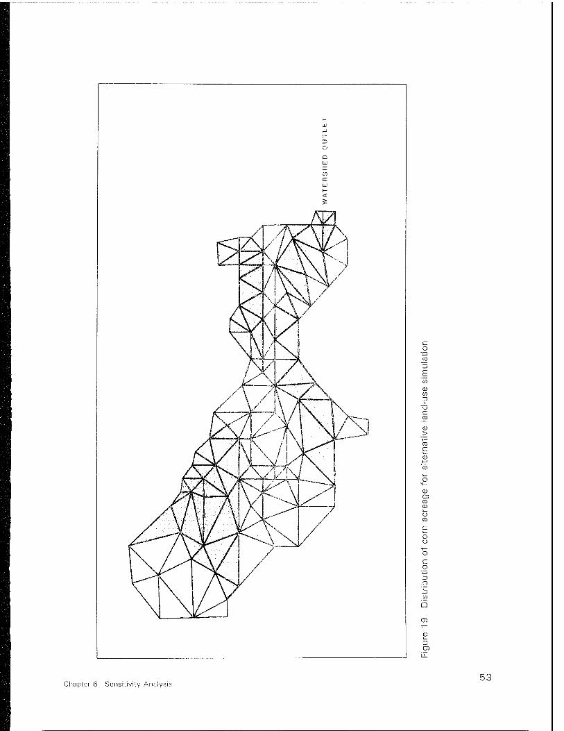
The amount of corn acreage was reduced from 2,500 to 1,900 ha. The majority of the acreage removed from corn production was located in the western and central sections of the watershed as seen in Figure 19. The net effect of reducing the acreage was to reduce the amount of atrazine applied in the watershed. The anticipated result of reducing the acreage was a reduction in the atrazine concentration at the locations where corn was no longer being
52 Chapter 6 Sensitivity Analysis
CO
3
CD CO
"O c
CD > co c CD
CD
CD a> co CD
o co
o o
c o
X)
13 a)
Chapter 6 Sensitivity Analysis 53
grown. The atrazine concentration profile for the watershed was evaluated at 966, 1056, and 1161 hr after application.
Figures 20-22 display the atrazine concentrations within the watershed at the 966-, 1056-, and 1161-hr time-steps, respectively. The output from the model followed the anticipated trend. The atrazine concentrations were reduced in areas where corn production had been eliminated. One of the most noticeable differences between the alternative land use and the base condition figures is the absence of atrazine in the western half of the watershed of the alternative land-use plots. Only the eastern section of the watershed in the alternative land-use figures indicated the presence of atrazine. This could be attributed to the selection of the location within the watershed to eliminate corn acreage. Corn acreage was only removed from the western and central portions of the watershed. The corn acreage in the eastern portion of the watershed was unchanged from the base condition. Overall, output from the alternative land-use simulation conforms to anticipated results.
Saturated hydraulic conductivity
The saturated hydraulic conductivity affects the rate of water flow through the soil and thus has a tremendous impact on contaminant transport. The saturated hydraulic conductivity used for the base condition was 0.2 m/hr. This value was increased to 0.4 m/hr for the sensitivity analysis. Doubling the saturated hydraulic conductivity increased the amount of water able to flow through the soil layers. Transport of the atrazine through the soil layers should likewise be increased.
Results from the simulation are given in Figures 23-25. Figure 23 shows the atrazine concentrations at the 966-hr time-step. Comparing this to the same time-step of the base conditions reveals that the amount of atrazine is greatly reduced using the increased saturated hydraulic conductivity. This effect is also seen in Figures 24 and 25 which present the results at the 1056- and 1161-hr time-steps, respectively. The atrazine concentrations decrease below detection limits at the 1161-hr time-step. The physical significance is that the transport of atrazine with the new conductivity allows for the material to be transported at a much greater rate. Thus, the observed concentrations of atrazine should decrease when compared to identical times of the base con- dition simulation. This corresponds to the observed phenomena.
Further analysis of the output generated from the simulation showed that the atrazine had leached to a greater depth than that of the base conditions. The atrazine had only leached to a depth of approximately 1.2 m. In the base conditions, it went to a depth of 30 m when the conductivity was doubled. The concentrations were spread over a greater area, thus the concentrations were further reduced. Therefore, it was concluded that the FEMWATER model produced expected results upon increasing the saturated hydraulic conductivity.
Chapter 6 Sensitivity Analysis 55
Distribution coefficient
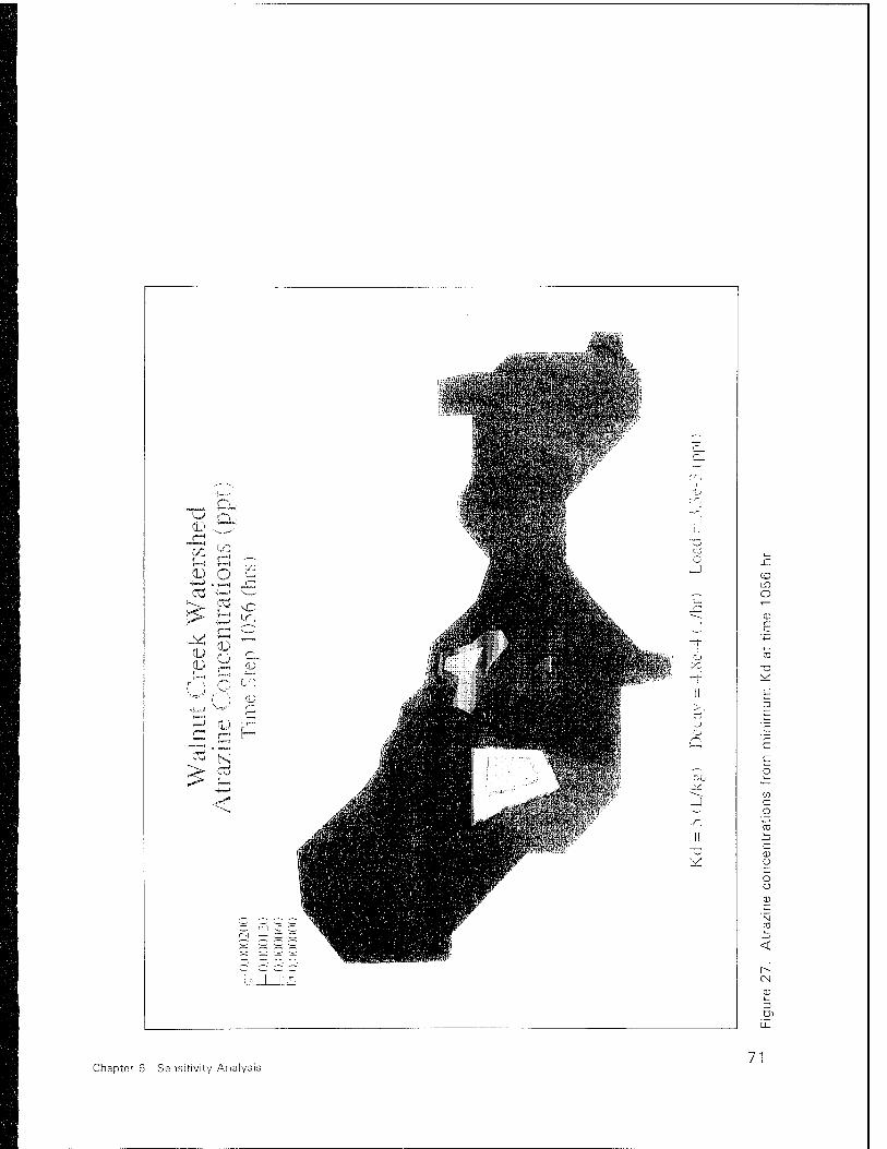
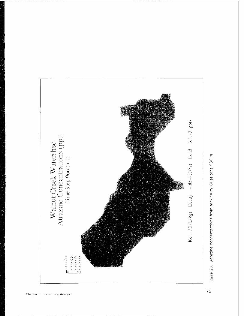
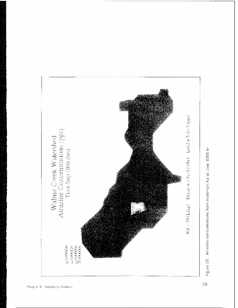
The distribution coefficient utilized for the base condition simulation was 10 L/kg. The value has been reported to range from a minimum of 5 to a maximum of 30 L/kg. These values were used for the sensitivity analysis. Figures 26-29 show the effects of altering the distribution coefficient. Fig- ures 26 and 27 depict the output produced^ incorporating the minimum distri- bution coefficient values at the time-steps of 966 and 1056 hr, respectively. Figures 28 and 29 display the changes utilizing the maximum value at the same respective time-steps.
Figures 26 and 27 show that the amount of atrazine in the watershed increases upon decreasing the distribution coefficient. The effect of decreas- ing the distribution coefficient was to reduce the amount of contaminant adsorbed to the surrounding soil. Therefore, the atrazine concentration should have increased based on the greater availability of the contaminant for trans- port. Conversely, increasing the distribution coefficient binds more contami- nant to the soil surface and less is available for transport. This effect was seen in Figures 28 and 29 when the maximum distribution coefficient was increased. The simulation output from utilizing the minimum and maximum distribution coefficients corresponded to expected results. Furthermore, it is clear that the distribution coefficient plays a significant role in the amount of contaminant transported in the watershed.
Decay constant
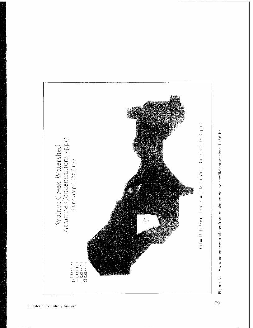
The decay constant in the transport simulation is responsible for reducing the amount of contaminant available for transport. The maximum decay con- stant for atrazine, 4.8E-4/hr, was used for the base condition simulation. A minimum decay constant of l.OE-4/hr was used for this sensitivity analysis. The anticipated result was to see more atrazine in the watershed. This was based on less chemical decay.
The results of the simulations with the minimum decay constant are given in Figures 30 and 31. Figure 30 represents the output from the 966-hr time- step and Figure 31 the ones from the 1056-hr time-step. The figures appear to be identical to the ones produced utilizing the maximum decay constant value. There do not appear to be any appreciable differences between the two sets of simulations. The anticipated result of an increase in atrazine concen- trations within the watershed was not observed.
The FEMWATER model does not appear to be very sensitive to the decay constant parameter. Use of the maximum and minimum decay constant values for the herbicide failed to reproduce any noticeable effects in the graphed output. In an effort to detect the amount of change that occurs from altering the decay constant parameter, the concentration was monitored at a selected node within the watershed and compared to the change produced from varying the distribution constant. The resulting information is given in Table 7. The
56 Chapter 6 Sensitivity Analysis

BS^^'4äsiu K Bm^^&|,
' *^^sl5l
ffl^ftr
rr,
CD -k**J 4%HH rrl
r*). ^ Cb il Ci T3
> £J '^ffiBMBHffi C i—( i—[ .—- &snn3SB , J Q-) O '/■-■
+-» -H = s« -5 T"
K*^ ^__i VQ
r^
k> G C^ ~t
reel
ne
e Sl
ep
1J oc
1! !>-■
■I^SBI^HMM
2 0-> i— O CJ
C r-i L -^Bj^nBa^^HBaBimBiB^BH G ' j • v—;
Co S3 trau
< j
riaül filpPlr ii HV ■^
C" ~i ^
ran
r-j g ~
IBM 7^1
CD CD CD
CD
E
CD -C ü cn CD co
"D c
0 > CO
c
c o
c CD O c o o CD c N CD
< O CN
CD
Chapter 6 Sensitivity Analysis 57

A^^\fe>^JliiL
äfiti
H fittfä c_
1 H^r^li^i;;' Cl- lip c~,
4—' «1 nn!fiHB9n«ES«§" '1j
™- Cu '«I WmßS r<~,
CD o' ■fciitHiK
ii
c/) <£j ■^ra KDK , ^ BKEffiHM,
CL) O £ jlilk. -J
Co ^~^ -—' ■7-
!> 4U ^ jJaBa [B|BH«B|HIHMPB|«8|IP^
,—-
. <—< o jsn|§,t.- *"-*'
eek
ep 1
■MJ 3HH IK. -t
'flilHMl u
r _. ^j -;—J BBMffilWmSj^ £ "Tf"
() o G0 jjfflBHwM|MMH>H
11 II
ti *"* E BHBKiBBHBffilHMiBlHHiMJiBKffi cz
^ 'D -r~ ö C t-'
o
Q CO fy] jj^^ KB|i > p 5.0 ^ ~j i -v
< Jim ^BBSI^^^^BHwmBBBffiltff*:
HHwF LJ
^
IfllB^^jiP fill
II
C: "l 9 ~ ^S rj —
8 8
"kl "ii^
CO LO o
CD
E
CD
E CD
_n o tf>
CD CO
CD >
CD
7c JZ
en c O
c CD cj
o o CD C
<
CN
CD
ZS CD
Chapter 6 Sensitivity Analysis 59

CD w
^ S-J ~ <L> O ■- ^ ■*-$ ~—-
Cv3 , ,
r-, co
f—1 ^
-**> N > a
<
mm
ITJJ;
_i
t—
CO
0 E
CD
E CD
CD (/) 3
X3
_C0
CD > en c CD
en c o
CD Ü C
o o
CD
C\j <N
CD
Chapter 6 Sensitivity Analysis

, ■#!.
';,ti ^-i^njKvWMSwiEfi^K^^i^^^h-
p.
—^ rr-
,- N ■j^^mwJMBW^^a^^T- 'lj ~L-~J r<~. i Q_( 'H r1""".
ii
!—I i—i .—. o
<D O ^ ■+—: •>—< p: 03 •*-> -= jBMl BlfflfiftlS§mrfa —
^-^ G3 S ' 499 j= KC i-[ ~o ^n raB§5&5i ~^ ^ ^ vO kj c c^
& £ B
t^H fef
-n-
CO
!—< r? GO BBSS WMBBJ^ ~~f
•-'iwraffi BBHH
II
3 <L> P o
Q t~-j . ^ cd Kj
^2 y??fffirowipBWM^BBHnBWM ■+-I gSMMJMBBHMfflBnMjfflfflB^^ •^~^
< JMB
II
5 r~\ c^ c^ ^Bffl
1002
)()(")
1
2 s ^läli 13' 1
CD CD en
CD
>
Ü 3
X3 C O O
X CD
E E o
tn c o
c CO u c o Ü cu c
CO CM
3 en
Chapter 6 Sensitivity Analysis 63
'° ol (-j ■
- Ö - <D o •-
■+—' - 7—i _c: Cvj 4-» —
p- £3 ^
^ a C) o & w r ) (u
CD ~~ o
~ cd +—i
<
ü- =
lü..LEU
Ml
II
_J
Q
II
CD LO O *—
CD
E
>
o D "a c o o
E 3
X CD
E E o
c o
c CD o c o Ü
CD C
CN
Chapter 6 Sensitivity Analysis 65

im
my
'+—> Jäiäj KjSßs3Bjr CL,
DC 8| BrafiJEJSS
^ ^ ^ £ A» l^^m llllp !—< !—< nSHSm.
dj O C/j
^Hülw 4—> ._H
cd +-> <—t
!>■ ^
jSjjSb,
i*^* ^_j vO ^äÜtn! ^BUgBBBBKBBBfi' rH i—i mBBBBuSB&iki
eek
icei
•laWfliBdlH
S—i *—i ■i—1 KH^M WBWiffiffnffimr^^^ Ur° 00 ^njmm HHMBHMHMnBIP'"*"^
E [HH^HB^^
Z> CD BMwIm MWMBBWWBMPBIJKSH
^_ H|HK( r—H .„, cd si
J2> cd «KII > Ui
4—1 Jgh HBBBHBMflBIBBaSc? *
<
KJ0
200
1001
20
\C
t^^oi
BBiBglr
IF flllr
BH ^ fl
B^yMiSnrwflqfwKIffv
i) i_
r<~, _c C"i *—
CD II *— « 03 O E
-t-J
■w ^— CD
> +J
.—■ > ■•— ■w
-1- o 3
13 T3 OQ C
o -1- ü
II
x CD
c/3 C o
c 03 o c o o CD c
Csl
D3
Ü.
Chapter 6 Sensitivity Analysis 67
J^^^
ji^SS^^S^^vw^Efc^ ^aw sMf'fv-
jägggj jmuMBMlfl MH^aM^^^^'-
H
-3 (
ppt)
-^ J U
p t ("r, <J P en <D r—H ii
4Z! ffl|^^|S^ro^öE: y G o
_J <& O c/: A—i ■ *—<
1—i
a -i—>
Cd ,—, ~
l<<^ J™< ^o ^ p**&~ 4—' ■o •—■
CD o (-1 CD
-J—>
■iSwrV^ Hütet "^ n^H co
r—i CO UHU Tf u O
U CD fl P Ii -'t—J' •—* c^
(-1 CD F o cu
*-G ^HNi^^^^^^H^Bfl^BB^Bn&fc^ C cd N B -,~^,IVr,.,:.);,^^nJI!|!l^lj||yj
£ cd ?—i -!—>
JH ^> r-^HBHQBfr7
... ■■ iiiiiBlmBmiffinH^i^^ < J HffSrV''' ■J^I
II j^HHR^i^p
£
c "i J c ^Qfl
)002
)00
l )(
)()(
) )(
)00
EäULÜß
CD CD CD
CD
E
"O
c 'c E E o
c o
c CD o c o Ü CD C
<
CD CN
CT) Li-
Chapter 6 Sensitivity Analysis 69
r-, o f~i
(L) ^™=
n IS1 Ü-J
r>H 1—1 - r~-
CD O • , 4-™» ( ' CTS -:_j ^_^
^ 03 !—i
<—'
ID CD o a.) <U <■ , -!——i 1—'
C ) n CO
U 0.) , j r—
t r— _> i ^ . ,_
H « * , >qi[Jij
03 N
<
*SnBP£WÄilä
vmm »HUfe
oo T3 -f- V
1! E Z)
— F u o c c E
E =JJ •~y * ^-^ en
_J c —- o ir, 4-'
cc 1! £:
c ■~> (11 X o
c o Ü
0 c
U:J_LE)
CD LO O
<
Chapter 6 Sensitivity Analysis 71
jmmalt
'«UHnfaftB^ls^ip ' — 3
H"-, ,—.
"!i
Q,, 39*HHr m
<-J K"' CD CT HBt en
II r-C -''^K^E^^' "O
ir> rr}, WSBIL «J
CL> O 7- 'JHWMSBBWK[^^I*-
4-—' - v—( " jffiWlHHMi^^^: —.
K"^ +-> >sO v^ C CJN
jl 111;' ,-c:
U o P" CD ^ Sd 3p ~r
1!
5 i> il O
J=i C IITIJJEJMIMBI^^ Q
^ 'N ,flHafflj^W(|BBBKK||iHHM
i^MBMM^^p^^- ^—' SSE?- ^^_
< >MI FfjMHffMffiflM -j
^XMBI r*",
MBHuiHtSWj
BHBBBnBHJBfflHiH ii
5 ~l r-i —
- - ^H HF
EL Mjä
CD CD CD
CD
£
E
E X CO
E o
c o
c CD o c o CJ
CD c
CO
CO CM
CD
CD
LL
Chapter 6 Sensitivity Analysis 73
^MBg^H
jf^jüijg JIM Mi 111«
HF 1J
CIL, JsS ilillllilil' rr
CD O :i-
1111 li
-4~=J „ „„-4 r—'
cu -<--; '-^- ~ b> '^ ^0 W|||W|^B4,, jz:
;>■ -.rJ ^ ^{3*ffifl — 1—< 0 '^ä^nSB '•—-
KJ 7- _ BajJEfi —J-
^ O ^ ■<3MSBOBH
pip ■'LJ
f) 6 « .JJHHIBHMMBMI II '""■' ( ) Qj __ +_> -=-- <~" lull ^^HH^^^S^BB9n9n^mHfiB^ ■üe
5 r'l > ■ — r^iifsgSB^^^HS^HH 0 0
Q 7~TBiiH u ,-~H BB^fljHSHBftffl^^^BWM^^^ ^cd KJ
^ F> 1 ' ^^SiBqm^ DJJ l^""- »-< HffiSH H '■' ■ ■" 1 Jilffl^^S'^v"' i ; V
-1—' 11 v...- •"Viliii^BBBStOL'Jü'^ '"*i 1 ^-^
< ,,^1 HMBB
■BBIF II
liBfllfflBMBBJBI «F
Cj
^BBtt^KBBS^BuUBSBt&r
" r- 1 5 = ^w I00(
c()<)( 2 s ^HB
& I _i:ä
CO Ln O
CD
E
CD
73
X CO
E E o
_o CO
c CD o
5 CJ
CD c
<
en
Chapter 6 Sensitivity Analysis 75

(1) _""
^-- c.
rT> Si 5"
~} o,) r„...
Ä
IIRP ^Ä v«-'iiS»fiK*S - üfMÄÖCi fiESK
'jgtife «i life. l^«si^ tSÜSsi^.'1
;|||§ i|§§||
iJiRB CD CD CD
CD
E
c CD
"o St
CD O Ü
CD Ü CD
C
E E o en c o
i
c CD Ü C O o CD C
'N
< d CO
3
Chapter 6 Sensitivity Analysis 77
<D z
<U O r~ w . _« ^ C-*S -i—' '■—■
►*<*"" J_J •£}
CD 1=S o'
C .)
^ F*
<
5|J
^
ti l. J:IFI
CD LO o
CD r~ C
C CD
CJ
CD O O
CG O CD
E c
c o
c CD ü c o o CD C
<
CO
CD
O)
Chapter 6 Sensitivity Analysis 79
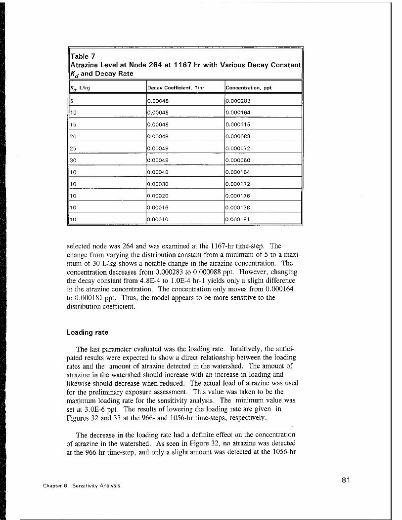
Table 7 Atrazine Level at Node 264 at 1167 hr with Various Decay Constant Kd and Decay Rate
Kd. L/kg Decay Coefficient, 1/hr Concentration, ppt
5 0.00048 0.000283
10 0.00048 0.000164
15 0.00048 0.000115
20 0.00048 0.000088
25 0.00048 0.000072
30 0.00048 0.000060
10 0.00048 0.000164
10 0.00030 0.000172
10 0.00020 0.000176
10 0.00016 0.000178
10 0.00010 0.000181
selected node was 264 and was examined at the 1167-hr time-step. The change from varying the distribution constant from a minimum of 5 to a maxi- mum of 30 L/kg shows a notable change in the atrazine concentration. The concentration decreases from 0.000283 to 0.000088 ppt. However, changing the decay constant from 4.8E-4 to 1.0E-4 hr-1 yields only a slight difference in the atrazine concentration. The concentration only moves from 0.000164 to 0.000181 ppt. Thus, the model appears to be more sensitive to the distribution coefficient.
Loading rate
The last parameter evaluated was the loading rate. Intuitively, the antici- pated results were expected to show a direct relationship between the loading rates and the amount of atrazine detected in the watershed. The amount of atrazine in the watershed should increase with an increase in loading and likewise should decrease when reduced. The actual load of atrazine was used for the preliminary exposure assessment. This value was taken to be the maximum loading rate for the sensitivity analysis. The minimum value was set at 3.0E-6 ppt. The results of lowering the loading rate are given in Figures 32 and 33 at the 966- and 1056-hr time-steps, respectively.
The decrease in the loading rate had a definite effect on the concentration of atrazine in the watershed. As seen in Figure 32, no atrazine was detected at the 966-hr time-step, and only a slight amount was detected at the 1056-hr
Chapter 6 Sensitivity Analysis 81
time-step. Thus, the expected direct relationship between loading rate and concentration of atrazine in the watershed was observed.
82 Chapter 6 Sensitivity Analysis

■ :• •••^tNa ^stsSKÖ''ii-';' -'öSJ^P*v :;■ •■W^Bplii^te,; •
'w^SÄ^Si^MlMPifep^
; j^^HMg^^iv« y C-
«m^B> ^r; .—. 'lli läSääBllPp'"' ■U
ii
Co
!-H a — cu o ^ •9BH»* -J
^ ':S -5 Jllilllllk- .
K^ +-J vo I
i^ !H C^
T) ^ ex ü £ B !—i "X1 C^
WBSB SSsisffil SsPI&;
c) o ;t m II *"\ O P 13 rj \ r™ o
£ c ^H^S^^ o ^
13'N W^gg^^^^m^mU ^2 ■4$M
HUH 5/j
T ' sBKBBm
< wBBBmS^m' _J ■jjfflmMMWJ »HP'' ■■PUP" II
S rN ^ ~H
1 ()()()(
:oo()( s THB HHSBHR
Dr I 1 ̂
CD CD
a) E
a) c
CD o
c E E o
c o
c CD o c o o CD c
CM CO
3
Chapter 6 Sensitivity Analysis 83

p..,
CD O '-
> £
CÜ
J__j *<—t
4_j V=r-
-^
CO
F~
^
•<
ill M »pi
-J
II
II
CO in O
en c
T3 to o
E 3 E c E E o
c o
c CD o c o u CD C
00 00
CD
Chapter 6 Sensitivity Analysis 85
7 Summary and Conclusions
The FEMWATER model demonstrates its flexibility and versatility of application in a wide range of real-world problems, including the simulation of flow alone, transport alone, as well as combined flow and transport problems. A robust, graphic interactive pre-processor and post-processor software has been implemented to support the model. It makes the sophisticated and complicated FEMWATER model simpler to use and able to address a variety of problems.
The simulated flow by the FEMWATER model in the drain tile system was under-predicted because of the installation of vertical drain pipes to drain the water in the depression areas directly into drain tiles. The chimney effect cannot be modeled by the model.
The preliminary exposure assessment was conducted to determine the effects of current land use practices and agrichemical applications on ground- water quality. The developed simulation plan examined the use of the herbicide atrazine during the 1992 growing season (6 April through 26 September). Utilizing the FEMWATER model, it was determined that the herbicide leached to a depth of approximately 1.2 m during the time span and was only found in the surface soil layer. No atrazine was found in any of the soil layers at the end of the simulation period.
A sensitivity analysis was conducted to determine the impacts of altering the land use, saturated hydraulic conductivity, distribution coefficient, decay constant, and loading rate parameters on the simulation output from the FEMWATER model. While not all of the analyses conducted are presented herein, a general summary of the trends and generated output were deter- mined. The analysis revealed that predicted concentrations of atrazine generated from the model upon altering the parameters were reasonable and represented the physical processes occurring within the watershed.
Overall, the FEMWATER model has been demonstrated to be an effective tool for evaluating the fate of nonpoint sources of pollution. The flow fields and transport results are consistent with those one would expect to observe. The GMS has been proven to increase model productivity greatly. This is accomplished by easily generating the input data and providing quick and easy analysis of results. Together, these tools provide a powerful and relatively
Chapter 7 Summary and Conclusions 87
easy-to-use tool for evaluating the effects of nonpoint source pollution, thereby allowing the analysis of alternative management schemes.
88 Chapter 7 Summary and Conclusions
References
Brigham Young University. (1994a). "GMS, groundwater modeling system reference manual," Engineering Computer Graphics Laboratory, Provo, UT.
Brigham Young University. (1994b). "WMS, watershed modeling system integrated hydrologic modeling reference manual," Engineering Computer Graphics Laboratory, Provo, UT.
Chen, G.L., Ashwood, T.L., and Yeh, G.T. (1988). "Simulation of groundwater flow in a pipeline trench network using a 3-dimensional finite element model of water flow through saturated-unsaturated media," Oak Ridge National Laboratory, Oak Ridge, TN. ORNL/RAP/LTR-88/45.
Dongian, A.S., Chinnaswamy, R.V., and Beyerlein, D.C. (1993). "Surface water exposure assessment for Walnut Creek, Iowa, preliminary applica- tion of the EPA hydrological simulation program — FORTRAN (HSPF) to assess agrichemical contribution and impacts," Final Review Draft. U.S. Environmental Protection Agency, Athens, GA.
Freeze, R.A., and Cherry, J.A. (1979). Groundwater. Prentice-Hall, Englewood Cliffs, NJ.
Haitjema, H.M., Mitchell-Bruker, S., and Kraemer, S.R. (1993). "Hierarchical approach to modeling surface-groundwater interactions: The Walnut Creek watershed in regional perspective," Agriculrural Research to protect water quality. Soil and Water Conservation Society, Ankery, IA.
Iowa State University, U.S. Department of Agriculture Soil Conservation Service, and the Iowa Department of Agriculture and Land Stewardship. (1990). "Iowa Soil Properties and Interpretations Data Base (ISPAID)."
Klingman, G.C., and Ashton, F.M. (1982). Weed Science Principles and Practices. John Wiley & Sons, NY, 237-249
Lin, H.C., and Yeh, G.T. (1995). "User's manual for the FEMWATER groundwater computer program: A three-dimensional finite element model of density-dependent flow and transport through saturated-unsaturated
References 89
porous media," U.S. Army Corps of Engineers Waterways Experiment Station, Vicksburg, MS.
Thompson, C. A. (1982a). "Ground-water resources of Boone County," State of Iowa Department of Natural Resources, Geological Survey Bureau, Des Moines, IA. Open file 82-85.
Thompson, C. A. (1982b). "Ground-water resources of Story County," State of Iowa Department of Natural Resources, Geological Survey Bureau, Des Moines, IA. Open file 82-85.
U. S. Geological Survey. (1987). "Digital elevation model," Reston, VA.
U.S. Geological Survey. (1991). "Letter report of driller's logs for the shallow observation wells in Boone and Story Counties," Iowa City, IA.
Yeh, G.T., Chang, J. R., Gwo, J. P., Lin, H.C., Richards, D. R., and Martin, W.D. (1994). "3DSALT: A three-dimensional finite element model of density-dependent flow and transport through saturated- unsaturated media," U.S. Army Corps of Engineers Waterways Experiment Station, Vicksburg, MS.
Yeh, G.T., Sharp-Hansen, S., Lester, B., Strobl, R., and Scarbrough, J. (1992). 3DFEMWATER/3DLEWASTE: Numerical codes for delineating wellhead protection areas in agricultural regions based on the assimilative capacity criterion, U.S. Environmental Protection Agency, Athens, GA. EPA/600/R-92/223.
Ward, A., Alberts, G., Anderson, J., Hatfield J., and Watts, D. (1993). "The management systems evaluation areas program: Data collection, management and exchange MSEA program internal document," USDA/CSRS/ARS, Ohio State University, Columbus, OH.
90 References

REPORT DOCUMENTATION PAGE Form Approved OMB No. 0704-0188
Public reporting burden for this collection of information is estimated to average 1 hour per response, including the time for reviewing instructions, searching existing data sources, gathering and maintaining the data needed, and completing and reviewing the collection of information. Send comments regarding this burden estimate or any other aspect of this collection of information, including suggestions for reducing this burden, to Washington Headquarters Services, Directorate for Information Operations and Reports, 1215 Jefferson Davis Highway, Suite 1204, Arlington, VA22202-4302, and to the Office of Management and Budget, Paperwork Reduction Project (0704-0188), Washington, DC20503.
1. AGENCY USE ONLY (Leave blank) 2. REPORT DATE September 1995
3. REPORT TYPE AND DATES COVERED Final report
4. TITLE AND SUBTITLE FEMWATER Usability for the EPA MASTER and Wellhead Protection Research Programs
5. FUNDING NUMBERS
6. AUTHOR(S) Hsin-chi Jerry Lin, Patrick Deliman, William D. Martin
7. PERFORMING ORGANIZATION NAME(S) AND ADDRESS(ES) U.S. Army Engineer Waterways Experiment Station 3909 Halls Ferry Road, Vicksburg, MS 39180-6199
Brigham Young University Provo,Utah 84601
8. PERFORMING ORGANIZATION REPORT NUMBER Technical Report HL-95-5
9. SPONSORING/MONITORING AGENCY NAME(S) AND ADDRESS(ES) U.S. Environmental Protection Agency Environmental Research Laboratory Athens, GA 30605
10. SPONSORING/MONITORING AGENCY REPORT NUMBER
11. SUPPLEMENTARY NOTES
Available from National Technical Information Service, 5285 Port Royal Road, Springfield, VA 22161.
12a. DISTRIBUTION/AVAILABILITY STATEMENT
Approved for public release; distribution is unlimited.
12b. DISTRIBUTION CODE
13. ABSTRACT (Maximum 200 words) Walnut Creek watershed is located within Boone and Story Counties of central Iowa. Walnut Creek has been extensively
monitored as part of the U.S. Environmental Protection Agency (EPA) Midwest Agricultural Surface and Subsurface Transport and Effects Research Program.
The objectives of this study were to demonstrate usability of the existing GMS to conduct a preliminary exposure assessment for agricultural chemicals used in the Walnut Creek watershed and to evaluate impacts of varying the agricultural
chemical load through sensitivity analysis of changes to model parameters.
Two three-dimensional (3-D) meshes of Walnut Creek watershed were created by GMS. One 3-D was an inset mesh of the subdrain tile system of the watershed. This mesh was used to test and evaluate schemes to represent the drain tile feature of the watershed. The other 3-D mesh was used to represent the entire watershed based on the best available data. This mesh
was used to study the movement of agricultural chemicals applied to the surface.
(Continued)
14. SUBJECT TERMS Agricultural chemicals transport Saturated and unsaturated porous media
Contaminant transport model Walnut Creek watershed
Groundwater flow model
15. NUMBER OF PAGES
98
16. PRICE CODE
17. SECURITY CLASSIFICATION OF REPORT UNCLASSIFIED
18. SECURITY CLASSIFICATION OF THIS PAGE UNCLASSIFIED
19. SECURITY CLASSIFICATION OF ABSTRACT
20. LIMITATION OF ABSTRACT
NSN 7540-01-280-5500 Standard Form 298 (Rev. 2-89) Prescribed by ANSI Std. Z39-18 298-102
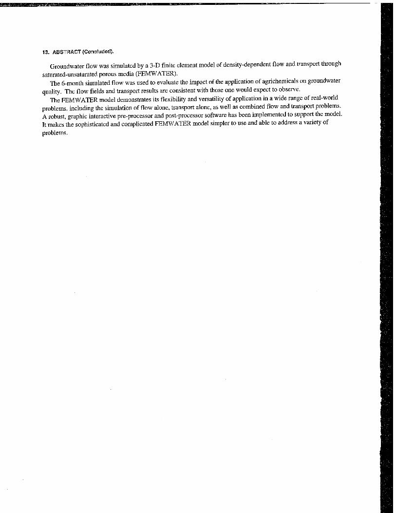
13. ABSTRACT (Concluded).
Groundwater flow was simulated by a 3-D finite element model of density-dependent flow and transport through saturated-unsaturated porous media (FEMWATER).
The 6-month simulated flow was used to evaluate the impact of the application of agrichemicals on groundwater quality. The flow fields and transport results are consistent with those one would expect to observe.
The FEMWATER model demonstrates its flexibility and versatility of application in a wide range of real-world problems, including the simulation of flow alone, transport alone, as well as combined flow and transport problems. A robust, graphic interactive pre-processor and post-processor software has been implemented to support the model. It makes the sophisticated and complicated FEMWATER model simpler to use and able to address a variety of
problems.