8Fermi Surfaces and Metals

8.1. Folding of the Brillouin zone

8.1.1. 1D

Fig. 1. Dispersion relation enk shown in extended zone, reduced zone and periodic zone. (Figure 4 in text book page 225).

8.1.2. 2DLet’s start by considering a very weak square lattice.

72 Phys463.nb

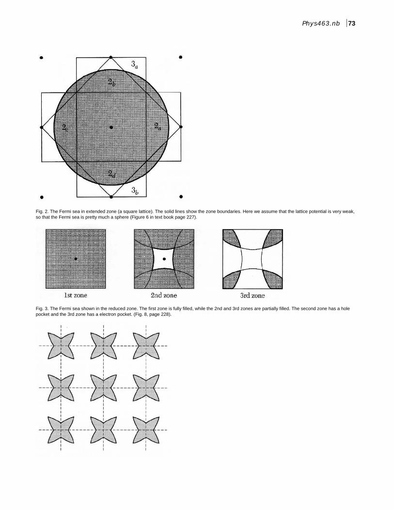
Fig. 2. The Fermi sea in extended zone (a square lattice). The solid lines show the zone boundaries. Here we assume that the lattice potential is very weak, so that the Fermi sea is pretty much a sphere (Figure 6 in text book page 227).

Fig. 3. The Fermi sea shown in the reduced zone. The first zone is fully filled, while the 2nd and 3rd zones are partially filled. The second zone has a hole pocket and the 3rd zone has a electron pocket. (Fig. 8, page 228).

Phys463.nb 73

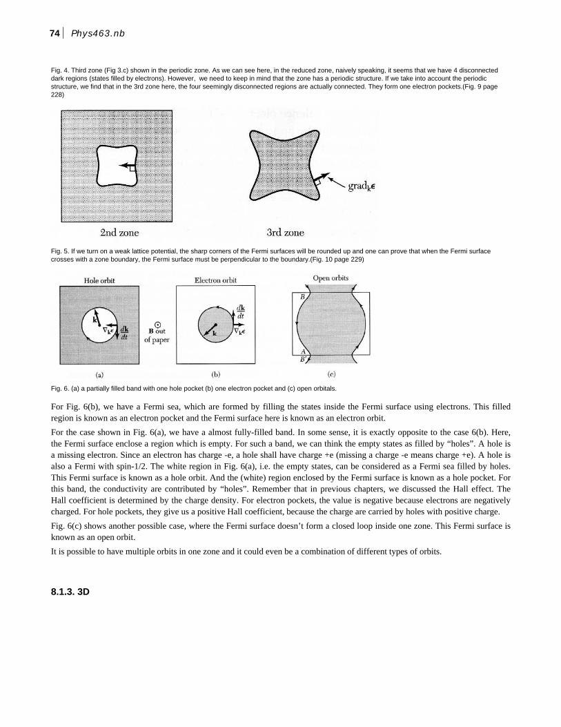
Fig. 4. Third zone (Fig 3.c) shown in the periodic zone. As we can see here, in the reduced zone, naively speaking, it seems that we have 4 disconnected dark regions (states filled by electrons). However, we need to keep in mind that the zone has a periodic structure. If we take into account the periodic structure, we find that in the 3rd zone here, the four seemingly disconnected regions are actually connected. They form one electron pockets.(Fig. 9 page 228)

Fig. 5. If we turn on a weak lattice potential, the sharp corners of the Fermi surfaces will be rounded up and one can prove that when the Fermi surface crosses with a zone boundary, the Fermi surface must be perpendicular to the boundary.(Fig. 10 page 229)

Fig. 6. (a) a partially filled band with one hole pocket (b) one electron pocket and (c) open orbitals.

For Fig. 6(b), we have a Fermi sea, which are formed by filling the states inside the Fermi surface using electrons. This filledregion is known as an electron pocket and the Fermi surface here is known as an electron orbit.

For the case shown in Fig. 6(a), we have a almost fully-filled band. In some sense, it is exactly opposite to the case 6(b). Here,the Fermi surface enclose a region which is empty. For such a band, we can think the empty states as filled by “holes”. A hole isa missing electron. Since an electron has charge -e, a hole shall have charge +e (missing a charge -e means charge +e). A hole isalso a Fermi with spin-1/2. The white region in Fig. 6(a), i.e. the empty states, can be considered as a Fermi sea filled by holes.This Fermi surface is known as a hole orbit. And the (white) region enclosed by the Fermi surface is known as a hole pocket. Forthis band, the conductivity are contributed by “holes”. Remember that in previous chapters, we discussed the Hall effect. TheHall coefficient is determined by the charge density. For electron pockets, the value is negative because electrons are negativelycharged. For hole pockets, they give us a positive Hall coefficient, because the charge are carried by holes with positive charge.

Fig. 6(c) shows another possible case, where the Fermi surface doesn’t form a closed loop inside one zone. This Fermi surface isknown as an open orbit.

It is possible to have multiple orbits in one zone and it could even be a combination of different types of orbits.

8.1.3. 3D

74 Phys463.nb

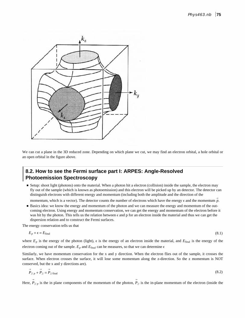
We can cut a plane in the 3D reduced zone. Depending on which plane we cut, we may find an electron orbital, a hole orbital oran open orbital in the figure above.

8.2. How to see the Fermi surface part I: ARPES: Angle-Resolved Photoemission Spectroscopy† Setup: shoot light (photons) onto the material. When a photon hit a electron (collision) inside the sample, the electron may

fly out of the sample (which is known as photoemission) and this electron will be picked up by an detector. The detector can distinguish electrons with different energy and momentum (including both the amplitude and the direction of the

momentum, which is a vector). The detector counts the number of electrons which have the energy e and the momentum pØ

.† Basics idea: we know the energy and momentum of the photon and we can measure the energy and momentum of the out-

coming electron. Using energy and momentum conservation, we can get the energy and momentum of the electron before it was hit by the photon. This tells us the relation between e and p for an electron inside the material and thus we can get the dispersion relation and to construct the Fermi surfaces.

The energy conservation tells us that

(8.1)Ep + e = Efinal

where Ep is the energy of the photon (light), e is the energy of an electron inside the material, and Efinal is the energy of the

electron coming out of the sample. Ep and Efinal can be measures, so that we can determine e

Similarly, we have momentum conservation for the x and y direction. When the electron flies out of the sample, it crosses thesurface. When electron crosses the surface, it will lose some momentum along the z-direction. So the z momentum is NOTconserved, but the x and y directions are).

(8.2)PØ

p + PØ

= PØ

final

Here, PØ

p is the in plane components of the momentum of the photon, PØ

is the in-plane momentum of the electron (inside the

Phys463.nb 75

material), and PØ

final is the momentum of the final electron flying away from the sample.

Combining the information obtained above, we get the energy and momentum (in plane) of an electron. There are more compli-

cated techniques that can provide us the z component of the electron. At the end of the day, we can get both e and PØ

, so we get

the dispersion relation ePØ. And we can get the Fermi surface by requiring epØ = m.

Limitations of ARPES:

† It is a surface probe: light cannot go deep into a metal, so we can only measure the electronic properties near the surface of the sample. For some materials, surface is pretty much the same as bulk, but for some other materials it isn't the case. There, what we see in ARPES may not reflect the true properties of the material in the bulk. So one need to be very careful about it.

† ARPES needs a very clean and flat surface (easier for layered materials but not easy for many other materials).

† One can only measure the dispersion relation for e § m. This is because we need to get one electron out of the sample from the quantum state with energy e and momentum p. This means that we can only see occupied states in ARPES. If the state is empty e > m, there is no electron, so we cannot see this state. This is also how m is determined in ARPES experiments. (There are techniques which allow us to see energy above the Fermi energy).

† The momentum resolution for Pz is lower than Px and Py.

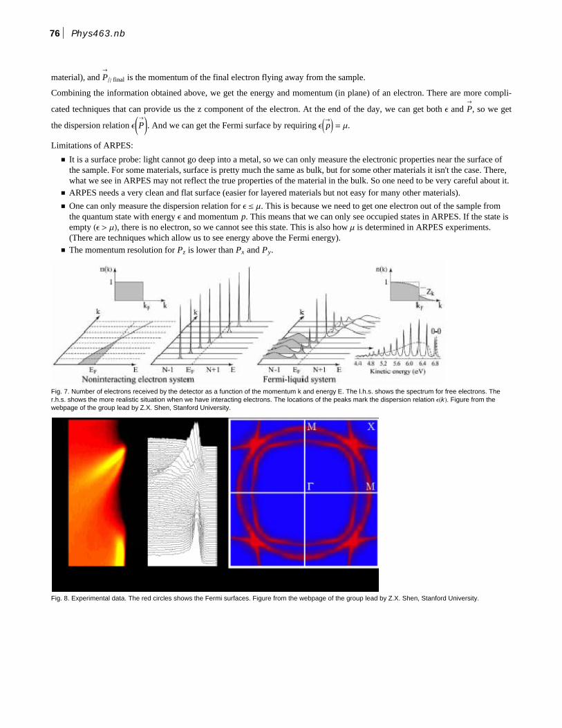
Fig. 7. Number of electrons received by the detector as a function of the momentum k and energy E. The l.h.s. shows the spectrum for free electrons. The r.h.s. shows the more realistic situation when we have interacting electrons. The locations of the peaks mark the dispersion relation ek. Figure from the webpage of the group lead by Z.X. Shen, Stanford University.

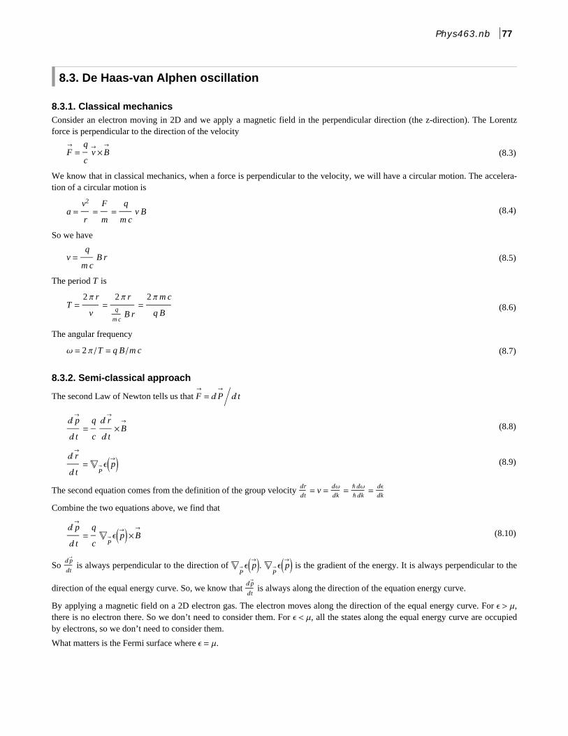
Fig. 8. Experimental data. The red circles shows the Fermi surfaces. Figure from the webpage of the group lead by Z.X. Shen, Stanford University.

76 Phys463.nb

8.3. De Haas-van Alphen oscillation

8.3.1. Classical mechanicsConsider an electron moving in 2D and we apply a magnetic field in the perpendicular direction (the z-direction). The Lorentzforce is perpendicular to the direction of the velocity

(8.3)FØ=

q

cvØμBØ

We know that in classical mechanics, when a force is perpendicular to the velocity, we will have a circular motion. The accelera-tion of a circular motion is

(8.4)a =v2

r=

F

m=

q

m cv B

So we have

(8.5)v =q

m cB r

The period T is

(8.6)T =2 p r

v=

2 p rq

m cB r

=2 pm c

q B

The angular frequency

(8.7)w = 2 p T = q B m c

8.3.2. Semi-classical approach

The second Law of Newton tells us that FØ= „P

Ø„ t

(8.8)„ pØ

„ t=

q

c

„ rØ

„ tμBØ

(8.9)„ rØ

„ t= !

PØ ep

Ø

The second equation comes from the definition of the group velocity „r

„t= v = „w

„k= Ñ „w

Ñ „k= „e

„k

Combine the two equations above, we find that

(8.10)„ pØ

„ t=

q

c!

PØ ep

ØμBØ

So „pØ

„t is always perpendicular to the direction of !

PØ ep

Ø. !PØ ep

Ø is the gradient of the energy. It is always perpendicular to the

direction of the equal energy curve. So, we know that „pØ

„t is always along the direction of the equation energy curve.

By applying a magnetic field on a 2D electron gas. The electron moves along the direction of the equal energy curve. For e > m,there is no electron there. So we don’t need to consider them. For e < m, all the states along the equal energy curve are occupiedby electrons, so we don’t need to consider them.

What matters is the Fermi surface where e = m.

Phys463.nb 77

8.3.3. Quantization condition for electrons at the Fermi surfaceThe Bohr-Sommerfeld quantization condition

(8.11) pØÿ„ rØ= 2 p Ñ n + g

where n is an integer and g is some fixed value, typically 1/2.

For a circular motion, this implies that

(8.12) pØÿ„ rØ=

2 p Ñ

l „ r =

2 p Ñ

l2 p r = 2 p Ñ n + g

If we ignore g, which is unimportant for the discussion below, this condition implies that

(8.13)2 p r

l= n

When we travel around the circle, we want the circumference being an integer times the wave length. If this condition is satisfied,the wave will have constructive inference when it travels around the circle.

Let’s come back to the equation of motion

(8.14)„ pØ

„ t=

q

c

„ rØ

„ tμBØ

So we have

(8.15)pØ=

q

crØμBØ+ constant

The constant part is unimportant, since we can always redefine the origin (the point which we called r = 0) to absorb the constant

into rØ

. So we have

(8.16)pØ=

q

crØμBØ

(8.17)pØμBØ=

q

crØμBØμB

Ø=

q

cBØr

ØÿBØ - r

ØBØ ÿBØ = -q

crØ

B2

(8.18)rØ= -

c

q

pØμBØ

B2

(8.19)„ rØ= -

c

q

„ pØμBØ

B2

(8.20)

pØÿ„ rØ= -

c

q p

Ø.„ pØμBØ

B2= -

c

q B2 p

Ø.„ p

ØμBØ =

-c

q B2 B

Ø.pØμ„ p

Ø = - c

q B p

Øμ„ p

Ø = - c

q BÑ2 k

Øμ„ k

Ø = - c

q BÑ2 S = 2 p Ñ n + g

where S is the area enclosed by the Fermi surface in the k-space.

(8.21)1

B= -2 p n + g q

c S Ñ

78 Phys463.nb

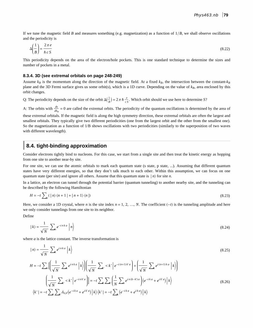
If we tune the magnetic field B and measures something (e.g. magnetization) as a function of 1 B, we shall observe oscillationsand the periodicity is

(8.22)D1

B=

2 p e

Ñ c S

This periodicity depends on the area of the electron/hole pockets. This is one standard technique to determine the sizes andnumber of pockets in a metal.

8.3.4. 3D (see extremal orbitals on page 248-249)Assume kB is the momentum along the direction of the magnetic field. At a fixed kB, the intersection between the constant-kB

plane and the 3D Fermi surface gives us some orbit(s), which is a 1D curve. Depending on the value of kB, area enclosed by thisorbit changes.

Q: The periodicity depends on the size of the orbit D 1

B = 2 p Ñ e

c S. Which orbit should we use here to determine S?

A: The orbits with „e„kB

= 0 are called the extremal orbits. The periodicity of the quantum oscillations is determined by the area of

these extremal orbitals. If the magnetic field is along the high symmetry direction, these extremal orbitals are often the largest andsmallest orbitals. They typically give two different periodicities (one from the largest orbit and the other from the smallest one).So the magnetization as a function of 1/B shows oscillations with two periodicities (similarly to the superposition of two waveswith different wavelength).

8.4. tight-binding approximation

Consider electrons tightly bind to nucleons. For this case, we start from a single site and then treat the kinetic energy as hoppingfrom one site to another near-by site.

For one site, we can use the atomic orbitals to mark each quantum state (s state, p state, ...). Assuming that different quantumstates have very different energies, so that they don’t talk much to each other. Within this assumption, we can focus on onequantum state (per site) and ignore all others. Assume that this quantum state is n for site n.

In a lattice, an electron can tunnel through the potential barrier (quantum tunneling) to another nearby site, and the tunneling canbe described by the following Hamiltonian

(8.23)H = -t n n n + 1 + n + 1 n

Here, we consider a 1D crystal, where n is the site index n = 1, 2, …, N . The coefficient -t is the tunneling amplitude and herewe only consider tunnelings from one site to its neighbor.

Define

(8.24)k = 1

N

n‰-Â n k a n

where a is the lattice constant. The inverse transformation is

(8.25)n = 1

N

k‰Â n k a k

(8.26)

H = -t n 1

N

k‰Â n k a k 1

N

k'< k ' ‰-Â n+1 k' a +

1

N

k‰Â n+1 k a k

1

N

k'< k ' ‰-Â n k' a = -t

k

k'

1

N

n‰Â n k-k' a ‰- k a + ‰Â k' a k

k ' = -t k

k'dk,k'‰- k a + ‰Â k' a k k ' = -t

k‰- k a + ‰Â k a k

Phys463.nb 79

k k k

k =k-2 t cosk a k k

It is easy to check that

(8.27)H k = -2 t cosk a kso |k is an eigenstate of the Hamiltonian and the corresponding eigen-energy is e k = -2 t cos k a with -p a < k < p a. This isone energy band.

The bottom line: If the atomic states are separated far from each other in energy (the energy difference is much larger than t),there is a one-to-one correspondence between atomic states in an atom and the energy bands. One atomic state (in each atom)gives us one band and one band comes from one atomic states. If the band comes from a s-orbital in an atom, we call it an s-band,p-orbitals form a p-band, etc.

80 Phys463.nb