JOURNAL OF

fhlancial ECONOMIES

ELSEVIER Journal of Financial Economics 43 (1997) 341 372

Detecting long-run abnormal stock returns: The empirical power and specification of test statistics

Brad M. B a r b e r * , John D. L y o n

Graduate School c~[ Management, University ~?[ Cal{[ornia Davis, Davis, CA 95616, USA

(Received November 1995: final version July 1996)

Abstract

We analyze the empirical power and specification of test statistics in event studies designed to detect long-run (one- to five-year) abnormal stock returns. We document that test statistics based on abnormal returns calculated using a reference portfolio, such as a market index, are misspecified (empirical rejection rates exceed theoretical rejection rates) and identify three reasons for this misspecification. We correct for the three identified sources of misspecification by matching sample firms to control firms of similar sizes and book-to-market ratios. This control firm approach yields well-specified test statistics in virtually all sampling situations considered.

Key words: Event studies; Firm size; Book4o-market ratios JEL classification: G 1 2 : G 1 4

1. Introduction

Many recent studies in financial economics analyze the long-run behavior of stock returns following major corporate events or decisions, such as divi- dend initiation, stock splits, acquisitions, or security offerings. In these studies, the post-event return performance of sample firms is tracked for a period of time following the event. There is considerable variation in the measures of abnormal returns and the statistical tests that empirical researchers use to detect

* Corresponding author.

Peter Hall, Chih-Ling Tsai, and David Rocke provided valuable insights on the statistical issued involved in this paper. We are grateful for the comments of Anup Agrawal, Sanjai Bhagat, Peter Clark, Masako Darrough, Eugene Fama (the referee), Paul Griffin, Prem Jain, Kathy Kahle, S.P. Kothari, Michael Maher. Wayne Mikkelson, Mark Nelson, Jay Ritter, Bill Schwert (the editor), Slew Hong Teoh, Russ Wern3ers, and seminar participants at Michigan. Oregon, and UC-Davis. All errors are our own.

0304-405X/97/$17.00 © 1997 Elsevier Science S.A. All rights reserved Pll S 0 3 0 4 - 4 0 5 X ( 9 6 ) 0 0 8 9 0 - 2

342 RM. Barber, J.D. Lyon/Journal qf Financial Economics 43 (1997) 341-372

long-run abnormal stock returns. While Brown and Warner (1980, 1985), Dyckman, Philbrick, Stephan, and Ricks (1984), and Campbell and Wasley (1993) all document the empirical specification and power of test statistics designed to detect abnormal stock returns, these studies focus on the characteristics of abnor- mal returns measured on a particular day or, at the most~ cumulated over several months. In contrast, our research documents the empirical power and specifica- tion of test statistics designed to detect long-run abnormal stock returns. Our analysis focuses on annual, three-year, and five-year returns. We argue that many of the common methods used to calculate long-run abnormal stock returns are conceptually flawed and/'or lead to biased test statistics.

We consider two main issues in tests designed to detect long-run abnormal stock returns. First, we consider the calculation of abnormal returns. We argue that researchers should calculate abnormal returns as the simple buy-and-hold return on a sample firm less the simple buy-and-hold return on a reference port- folio or control firm. We document the biases that are induced by summing daily or monthly abnormal returns (referred to in the financial economics literature as cumulative abnormal returns). Second, we empirically evaluate the performance of three approaches for developing a benchmark for long-run stock returns. The first approach employs the return on a reference portfolio to calculate abnormal returns. The second approach matches sample firms to control firms on specified finn characteristics. The third approach is an application of the three-factor model of Fama and French (1993). We document the empirical power and specification of test statistics designed to detect long-run abnormal stock returns based on dif- ferent methods of calculating long-run abnormal returns and different approaches for developing a long-run return benchmark. Our analysis focuses on the annual, three-year, and five-year returns of firms listed on the New York, American, and NASDAQ exchanges with available data on the monthly return files maintained by the Center for Research in Security Prices (CRSP) from July 1963 through December 1994.

Our empirical results yield two insights. First, we document that using reference portfolios, such as an equally weighted market index or size decile portfolios, to calculate long-run abnormal returns is problematic. In general, abnormal returns calculated using reference portfolios yield test statistics that are misspecificed (empirical rejection rates exceed theoretical rejection rates). In Section 2, we identify and discuss in detail three reasons for the observed biases in test statistics. In brief, these three biases include:

• new l ist ing bias, which arises because in event studies of long-run abnormal returns, sampled firms generally have a long post-event history of returns, while firms that constitute the index (or reference portfolio) typically include new firms that begin trading subsequent to the event month;

• reba lanc in9 bias, which arises because the compound returns of a refer- ence portfolio, such as an equally weighted market index, are typically

B.M. Barber, ,I.D. Lyon/Journal of Financial Economics 43 (1997) 341-372 343

calculated assuming periodic (generally monthly) rebalancing, while the re- turns of sample firms are compounded without rebalancing; and

• skewness bias, which arises because long-run abnormal returns are positively skewed.

We find that cumulative abnormal returns (summed monthly abnormal returns) yield positively biased test statistics, while buy-and-hold abnormal returns (the compound return on a sample firm less the compound return on a reference portfolio) yield negatively biased test statistics. These apparently contradictory results occur because of the differential impact of the new listing, rebalancing, and skewness biases on cumulative abnormal returns and buy-and-hold abnormal returns.

The second insight to emerge from our analysis is the efficacy of a control firm approach for detecting long-run abnormal stock returns. We document that matching sample firms to control firms of similar sizes and book-to-market ratios yields test statistics that are well specified in virtually all sampling situations that we consider. This control firm approach yields well-specified test statistics because it alleviates the new listing, rebalancing, and skewness biases.

Kothari and Warner (1996) also analyze the properties of long-run abnormal returns. Both our work and that of Kothari and Warner highlight the problems associated with calculating long-run abnormal returns using either a reference portfolio approach (which is discussed in detail in our work) or an application of an asset pricing model (which is discussed in detail by Kothari and Warner). However, we show that the control firm approach to calculating abnormal returns is robust to virtually all sampling situations that we consider. Though we highlight important differences between the two studies in this analysis, Barber and Lyon (1996a) thoroughly document all of the differences and their implications.

The remainder of this paper is organized as follows. In Section 2, we discuss sources of bias in the calculation of long-run abnormal returns. We discuss the return data, the construction of reference portfolios, and the application of the Fama-French three-factor model in Section 3. The calculation of cumulative ab- normal returns, buy-and-hold abnormal returns, our empirical methods, and the statistical tests that we use are defined in Section 4. Results are presented in Section 5. We discuss tests of median abnormal returns in Section 6. We close the paper in Section 7 with specific recommendations about the calculation of long-run abnormal returns.

2. The calculation of long-run abnormal returns

The convention in much of the research that analyzes abnormal returns has been to sum either daily or monthly abnormal returns over time. Define R~t as the month t simple return on a sample firm, E(Rir ) as the month t expected return

344 B.M. Barber, J.D. Lyon~Journal of Financial Economics 43 (1997) 341 372

for the sample firm, and ARit = Rit - E(Rit) as the abnormal return in month t. Cumulating across T periods yields a cumulative abnormal return (CAR):

T

C~RiT = Z ARit • I 1

(1)

In contrast, the return on a buy-and-hold investment in the sample firm less the return on a buy-and-hold investment in an asset/portfolio with an appropriate expected return (BHAR) is

8mR, = IZl + lJl II + l--1 t=l

(2)

In this section, we discuss issues that lead to biases in the calculation of test statistics designed to detect long-run abnormal stock returns. Later, we consider several alternative methods of arriving at an expected return for a sample firm. However, in this section, for purposes of discussion, we consider the return on an equally weighted market index (Rmt) a s the expected return for each security. When we present our empirical results, we consider how the various biases affect the calculation of long-run abnormal returns when alternative expectation models are employed.

2.1. Cumulative abnormal returns ¢ CARs)

Ritter (1991) was among the first to argue that CARs and BHARs can be used to answer different questions. Consider the case of a 12-month CAR and an annual BHAR. Dividing the 12-month CAR by 12 yields a mean monthly abnormal return. Thus, a test of the null hypothesis that the 12-month CAR is zero is equivalent to a test of the null hypothesis that the mean monthly abnormal return of sample firms during the event year is equal to zero; it is not a test of the null hypothesis than the mean annual abnormal return is equal to zero. To test the latter hypothesis, a researcher needs to use the annual BHAR.

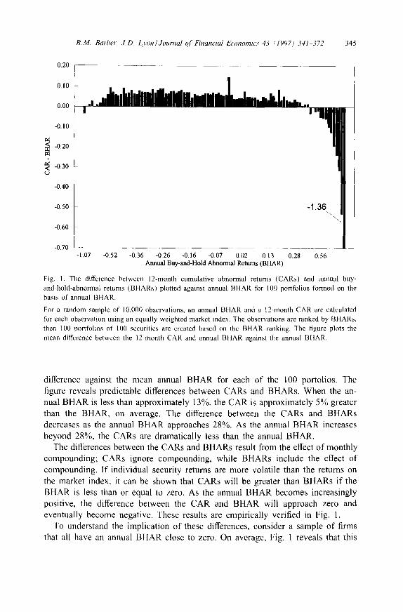
The difference between these two hypothesis tests can be understood by con- sidering the difference between CARs and BHARs. We randomly sample 10,000 observations between July 1963 and December 1993 from the CRSP NASDAQ and NYSE/AMEX monthly return files. (The data set used in this research is discussed in detail in Section 3.) We calculate a 12-month CAR and an annual BHAR using the CRSP NYSE/AMEX/NASDAQ equally weighted market index for each of the 10,000 observations. These 10,000 observations are then ranked into 100 portfolios of 100 securities each on the basis of their annual BHAR. This ranking creates the maximum spread in the annual BHAR. For each of the 100 portfolios, we calculate the mean difference between the cumulative and buy-and-hold abnormal returns (CARiT - B H A R i ; ) . In Fig. 1, we plot this mean

0.20

0.10 I 0.00

"0.10

"~ -0.20

t

-0.30 L )

B.M. Barber, J.D. Lyon~Journal of Financial Economics 43 (1997) 341-372 345

-0.40

"0.50

-0.60

-0.70

-1.36

! -1.07 -0.52 "0.36 -0.26 "0.16 -0.07 0.02 013 0.28 0.56

Annual Buy-and-Hold Abnormal Returns (BHAR)

Fig. 1. The difference between 12-month cumulative abnormal returns (CARs) and annual buy- and-hold-abnormal returns (BHARs) plotted against annual BHAR for 100 portfolios formed on the basis of annual BHAR.

For a random sample of 10,000 observations, an annual BHAR and a 12-month CAR are calculated for each observation using an equally weighted market index. The observations are ranked by BHARs, then 100 portfolios of 100 securities are created based on the BHAR ranking. The figure plots the mean difference between the 12-month CAR and annual BHAR against the annual BHAR.

difference against the mean annual BHAR for each of the 100 portolios. The figure reveals predictable differences between CARs and BHARs. When the an- nual BHAR is less than approximately 13%, the CAR is approximately 5% greater than the BHAR, on average. The difference between the CARs and BHARs decreases as the annual BHAR approaches 28%. As the annual BHAR increases beyond 28%, the CARs are dramatically less than the annual BHAR.

The differences between the CARs and BHARs result from the effect of monthly compounding; CARs ignore compounding, while BHARs include the effect of compounding. If individual security returns are more volatile than the returns on the market index, it can be shown that CARs will be greater than BHARs if the BHAR is less than or equal to zero. As the annual BHAR becomes increasingly positive, the difference between the CAR and BHAR will approach zero and eventually become negative. These results are empirically verified in Fig. 1.

To understand the implication of these differences, consider a sample of firms that all have an annual BHAR close to zero. On average, Fig. 1 reveals that this

346 B.M. Barber, ,LD. Lyon~Journal of Financial Economics 43 (1997) 341~72

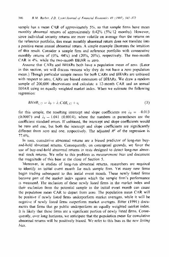
sample has a mean CAR of approximately 5%, so that sample firms have mean monthly abnormal returns of approximately 0.42% (5%/12 months). However, since individual security returns are more volatile on average than the returns on the reference portfolio, this mean monthly abnormal return does not translate into a positive mean annual abnormal return. A simple example illustrates the intuition of this result. Consider a sample firm and reference portfolio with consecutive monthly returns of (0%, 44%) and (20%, 20%), respectively. The two-month CAR is 4%, while the two-month BHAR is zero.

Assume that CARs and BHARs both have a population mean of zero. (Later in this section, we will discuss reasons why they do not have a zero population mean.) Though particular sample means for both CARs and BHARs are unbiased with respect to zero, CARs are biased estimators of BHARs. We draw a random sample of 200,000 observations and calculate a 12-month CAR and an annual BHAR using an equally weighted market index. When we estimate the following regression:

BHARi, 12 = 2o + 21CARi, 12 ÷ ~;i (3)

for this sample, the resulting intercept and slope coefficients are 20 = -0.013 (0,0007) and )q = 1.04l (0.0014), where the numbers in parentheses are the coefficient standard errors. If unbiased, the intercept and slope coefficients would be zero and one, but both the intercept and slope coefficients are significantly different from zero and one, respectively. The adjusted R 2 of the regression is 77.6%.

In sum, cumulative abnormal returns are a biased predictor of long-run buy- and-hold abnormal returns. Consequently, on conceptual grounds, we favor the use of buy-and-hold abnormal returns in tests designed to detect long-run abnor- mal stock returns. We refer to this problem as measuremen t bias and document the magnitude of this bias at the close of Section 5.

Moreover, in studies of long-run abnormal returns, researchers are required to identify an initial event month for each sample firm. Yet many new firms begin trading subsequent to this initial event month. These newly listed firms become part of the market index against which the sample firm's performance is measured. The inclusion of these newly listed firms in the market index and their exclusion from the potential sample in the initial event month can cause the population mean CAR to depart from zero. The population mean CAR will be positive if newly listed firms underperform market averages, while it will be negative if newly listed firms outperform market averages. Ritter (1991) docu- ments that firms that go public underperform an equally weighted market index. It is likely that these firms are a significant portion of newly listed firms. Conse- quently, over long horizons, we anticipate that the population mean for cumulative abnormal returns will be positively biased. We refer to this bias as the new listing

bias.

B.M. Barber, £D. Lyon~Journal of Financial Economics 43:1997) 341 372 347

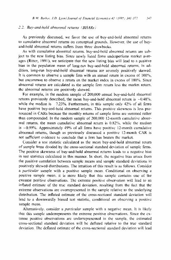
2.2. Buy-and-hoM abnormal returns (BHARs)

As previously discussed, we favor the use of buy-and-hold abnormal returns to cumulative abnormal returns on conceptual grounds. However, the use of buy- and-hold abnormal returns suffers from three drawbacks.

As with cumulative abnormal returns, buy-and-hold abnormal returns are sub- ject to the new listing bias. Since newly listed firms underperform market aver- ages (Ritter, 1991), we anticipate that the new listing bias will lead to a positive bias in the population mean of long-run buy-and-hold abnormal returns. In ad- dition, long-run buy-and-hold abnormal returns are severely positively skewed. It is common to observe a sample firm with an annual return in excess of 100%, but uncommon to observe a return on the market index in excess of 100%. Since abnormal returns are calculated as the sample firm return less the market return, the abnormal returns are positively skewed.

For example, in the random sample of 200,000 annual buy-and-hold abnormal returns previously described, the mean buy-and-hold abnormal return is -0.48%, while the median is -7.23%. Furthermore, in this sample only 42% of all firms have positive buy-and-hold abnormal returns. This positive skewness is less pro- nounced in CARs because the monthly returns of sample firms are summed rather than compounded. In the random sample of 200,000 12-month cumulative abnor- mal returns, the mean cumulative abnormal return is 0.82%, while the median is -0.99%. Approximately 49% of all firms have positive 12-month cumulative abnormal returns, though as previously discussed a positive 12-month CAR is not sufficient evidence to conclude that a firm has beaten the market.

Consider a test statistic calculated as the mean buy-and-hold abnormal return of sample firms divided by the cross-sectional standard deviation of sample firms. The positive skewness of buy-and-hold abnormal returns leads to a negative bias in test statistics calculated in this manner. In short, the negative bias arises from the positive correlation between sample means and sample standard deviations in positively skewed distributions. The intuition of this result is as follows. Consider a particular sample with a positive sample mean. Conditional on observing a positive sample mean, it is more likely that this sample contains one of the extreme positive observations. The extreme positive observation will lead to an inflated estimate of the true standard deviation, resulting from the fact that the extreme observations are overrepresented in the sample relative to the underlying distribution. The inflated estimate of the cross-sectional standard deviation will lead to a downwardly biased test statistic, conditional on observing a positive sample mean.

Alternatively, consider a particular sample with a negative mean. It is likely that this sample underrepresents the extreme positive observations. Since the ex- treme positive observations are underrepresented in the sample, the estimated cross-sectional standard deviation will be deflated relative to the true standard deviation. The deflated estimate of the cross-sectional standard deviation will lead

348 B.M. Barber, J.D. Lyon/Journal o[Finaneial Economies 43 (1997) 341-372

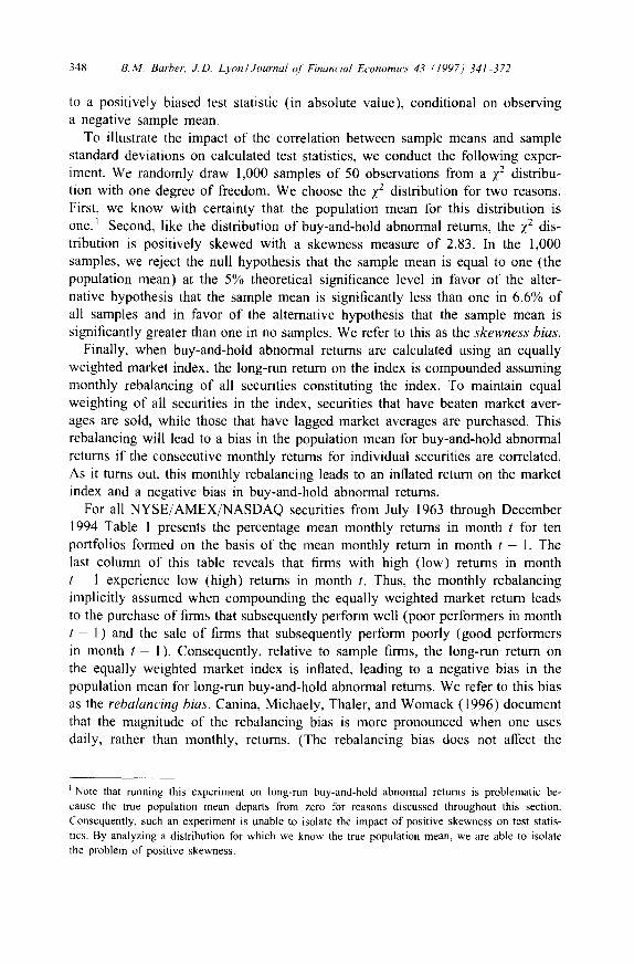
to a positively biased test statistic (in absolute value), conditional on observing a negative sample mean.

To illustrate the impact of the correlation between sample means and sample standard deviations on calculated test statistics, we conduct the following exper- iment. We randomly draw 1,000 samples of 50 observations from a )~2 distribu- tion with one degree of freedom. We choose the ~,2 distribution for two reasons. First, we know with certainty that the population mean for this distribution is one. 1 Second, like the distribution of buy-and-hold abnormal returns, the Z 2 dis- tribution is positively skewed with a skewness measure o f 2.83. In the 1,000 samples, we reject the null hypothesis that the sample mean is equal to one (the population mean) at the 5% theoretical significance level in favor of the alter- native hypothesis that the sample mean is significantly less than one in 6.6% of all samples and in favor of the alternative hypothesis that the sample mean is significantly greater than one in no samples. We refer to this as the skewness bias.

Finally, when buy-and-hold abnormal returns are calculated using an equally weighted market index, the long-run return on the index is compounded assuming monthly rebalancing of all securities constituting the index. To maintain equal weighting of all securities in the index, securities that have beaten market aver- ages are sold, while those that have lagged market averages are purchased. This rebalancing will lead to a bias in the population mean for buy-and-hold abnormal returns if the consecutive monthly returns for individual securities are correlated. As it turns out, this monthly rebalancing leads to an inflated return on the market index and a negative bias in buy-and-hold abnormal returns.

For all NYSE/AMEX/NASDAQ securities from July 1963 through December 1994 Table 1 presents the percentage mean monthly returns in month t for ten portfolios formed on the basis o f the mean monthly return in month t - 1. The last column of this table reveals that firms with high (low) returns in month t 1 experience low (high) returns in month t. Thus, the monthly rebalancing implicitly assumed when compounding the equally weighted market return leads to the purchase of firms that subsequently perform well (poor performers in month t - 1 ) and the sale o f firms that subsequently perform poorly (good performers in month t - 1). Consequently, relative to sample firms, the long-run return on the equally weighted market index is inflated, leading to a negative bias in the population mean for long-tun buy-and-hold abnormal returns. We refer to this bias as the rebalancing bias. Canina, Michaely, Thaler, and Womack (1996) document that the magnitude of the rebalancing bias is more pronounced when one uses daily, rather than monthly, returns. (The rebalancing bias does not affect the

I Note that running this experiment on long-run buy-and-hold abnormal returns is problematic be- cause the true population mean departs from zero for reasons discussed throughout this section. Consequently, such an experiment is unable to isolate the impact of positive skewness on test statis- tics. By analyzing a distribution for which we know the true population mean, we are able to isolate the problem of positive skewness.

B.M. Barber. J.D. Lyon~Journal of Financial Economics 43 (1997) 341 372 349

Table l Percentage arithmetic mean monthly returns in months t and t I of NYSE/AMEX/NASDAQ Firms sorted into deciles on the basis of monthly return in t - 1

In each month from July 1963 through December 1994 all firm-month returns are sorted into deciles based on the return in month t - 1. The mean return for finns in each decile is then calculated in month t.

Month t - 1 (%) mean (%) mean return decile return in t 1 return in t

1 (Low) -20.50 3.26 2 -10.08 1.54 3 -6.06 1.36 4 3.30 1.31 5 1.03 1.31 6 1.20 1.18 7 3.67 1.12 8 6.80 0.99 9 11.74 0.74

10 (High) 30.00 0.15

calculat ion o f cumula t ive abnormal returns, since the month ly returns o f sample

firms and the index are both summed rather than compounded . )

These return reversals do not necessar i ly indicate a profitable trading strategy.

Assume that firms with high ( low) returns in month t 1 are more l ikely to

have a c losing transaction at the posted ask (bid) price, but are equal ly l ikely

to have a c losing transaction at the bid or ask price in period t. This b i d ~ s k

bounce can at least partially explain the return reversals that we document . B lume

and Stambaugh (1983) analyze the effect o f the b id -a sk bounce on the small firm

premium. Conrad and Kaul (1993) and Ball, Kothari , and Was ley (1995) analyze

the implicat ions for contrarian strategies. Roll (1983) also documents that even

absent the b id -ask bounce, nonsynchronous trading can lead to negat ive serial

dependence in returns.

In summary, cumula t ive abnormal returns are subject to a measuremen t bias, a

new listing bias, and a skewness bias, a l though we document that the skewness

bias is less severe tbr cumula t ive abnormal returns than for buy-and-hold abnor-

mal returns. Buy-and-hold abnormal returns are subject to a new listing bias, a

skewness bias, and a rebalancing bias.

2.3. Continuously compounded vs. simple returns

The empir ical analysis in this paper is based on returns calculated as the change

in price plus dividends scaled by the beginning-of -per iod price, which we refer to

as the simple return. Cont inuous ly compounded returns yield inherently negat ive ly

350 IRM Barber, J.D. Lyon~Journal ~! Financial Economics 43 (1997) 341-372

biased estimates of long-run abnormal returns. The negative bias occurs because there is considerable cross-sectional variation in the returns of common stocks.

Consider a market with two securities, A and B. Securities A and B earn simple annual returns of 20% and 10%, respectively. An equally weighted in- dex of the two securities earns a simple annual return of 15%. The buy-and- hold abnormal returns for A and B are + 5% and - 5 % , respectively, and the mean abnormal return for the two securities is zero. In contrast, the continu- ously compounded returns for securities A and B are 18.2% and 9.5%, while the continuously compounded return on an equally weighted index is 14.0%. Using continuously compounded returns to calculate abnormal returns yields an abnormal return of +4.2% for A and - 4 . 5 % for B. The mean continuously compounded abnormal return for the two securities is - 0.3%. In fact, only when all securities that constitute an index have equal simple returns will the continu- ously compounded abnormal returns across all securities sum to zero. Otherwise, the mean continuously compounded abnormal return will be negative. For this reason, we object to the use of continously compounded returns for analyzing long-run return performance.

3. The returns data

In this section, we describe the data set that we use in our empirical analy- sis and discuss alternatives to the use of an equally weighted market index for calculating long-run abnormal stock returns.

3.1. Definin9 the population

Our analysis begins with all NYSE/AMEX/NASDAQ firms with available data on the monthly return files created by CRSP. Between July 1963 and December 1994 there are 1,798,509 firm-month returns. We begin in July 1963 because we require Compustat data on the book value of common equity, which is not generally available prior to 1962. Since event studies of long-run returns focus on the common stock performance of corporations we delete the firm-month returns on securities identified by CRSP as other than ordinary common shares (CRSP share codes 10 and 11). Thus, for example, we exclude from our analysis returns on American Depository Receipts, closed-end funds, foreign-domiciled firms, Primes and Scores, and real estate investment trusts.

Fama and French (1992) document that common stock returns are related to firm size and book-to-market ratios. In developing a test to detect long-run abnormal stock returns, we anticipate that it will be important to control for firm size and book-to-market ratios. As in Fama and French (1992, 1993), we measure firm size in June of each year as the market value of common equity (shares outstanding multiplied by June closing price). Size rankings based on market

B.M. Barber, J,D. Lyon/Journal o/'Financial Economics 43 (1997) 341 372 351

value of equity in year t are then used from July o f year t through June o f year t + 1. Thus, we further delete from our analysis firm-month returns from July o f year t through June of year t + 1 without a size ranking in June of year t.

As in Fama and French (1992, 1993), we measure a firm's book-to-market ratio using the book value of common equity (Compustat data item 60) reported on the firm's balance sheet in year t - 1 divided by the market value o f common equity in December of year t - 1. Rankings based on book-to-market ratios are then used from July o f year t through June of year t + 1. The calculation of book-to-market ratios precedes their use for ranking purposes by a minimum of six months to allow for delays in the reporting of financial statements by corporations. Thus, we further delete from our analysis firm-month returns from July o f year t through June of year t + 1 without a book-to-market ranking in year t - 1. We also delete firms that report a book value of common equity that is less than or equal to zero, though this is relatively rare. Previous drafts of this paper excluded financial firms from the analysis, but the general tenor of the results was not affected.

Table 2 reconciles the firm-month returns reported on CRSP between July 1963 and December 1994 to our final population of over 1.1 million firm-month returns. The majority of the finn-month returns lost from our analysis are deleted as a result o f requiring prior book-to-market data. We discuss the implication of this requirement at the close of this section. The 1.1 million firm-month returns correspond to the possible event months from which a researcher can draw a sample observation in a long-run event study.

In the remainder of this section, we consider three approaches for evaluat- ing the returns o f samples finns: a reference portfolio approach, a control finn

Table 2 Reconciliation of CRSP N Y S E AMEX/NASDAQ firm-month returns to our final population of firm-

month returns on the ordinary common stock of firms with market value of equity in June of year t

and book-to-market ratio in year t - 1: July 1963 to December 1994

Number of

Description firm-month returns

All valid firm-month returns

Less: Firm-month returns for other than ordinary common stock

Firm-month returns without a book-to-market ranking in year t - 1

(but with a size ranking in year t)

Firm-month returns without a size ranking in year t and without a book-to-market ranking in year t - 1

1,798,509

136.849

397,411

85,574

Final population of firm-month returns 1,178,675

352 BM. Barber, J.D. Lyon~Journal o[Financial Economics 43 (1997) 341 372

approach, and an application of the Fama-French three-factor model. Though financial economists have long recognized the importance of controlling for firm size in the calculation of long-run abnormal stock returns (see, for example, Dimson and Marsh, 1986), only recently have researchers controlled for both size and book-to-market patterns in studies that analyze long-run abnormal re- turns. While we develop and analyze reference portfolios and control firms based on size alone, we anticipate (and our results confirm) that in certain sampling situations it is critical to control for both size and book-to-market patterns in common stock returns.

In Table 3, we summarize many of the recent studies of long-run abnormal stock return performance following major corporate events and the benchmarks

Yablc 3 Summary of studies analyzing long-run abnormal stock returns following corporate events or decisions

Author(s) Corporate event studied Return benchmark

Bernard and Thomas (1989)

Ritter ( 1991 )

Agrawal, Jaffe. and Mandelker ( 1992 )

Womack (1996)

Ikenberry, Lakonishok, and Vermaelen (1995)

Loughran and Ritter (1995)

Spiess and Affleck- Graves ( 1995 )

Michaely, Thaler. and Womack (1995)

Desai and Jain (1996)

Earnings announcements

Initial public offerings

Acquisitions

Analyst recommendations

Share repurchase

Initial public and Seasoned equity' offerings

Seasoned equity' offerings

Dividend initiation and omission

Stock splits and dividends

Market model ~

Market index Size/industry control finn Size portfolio

Size portfolio

Size portfolio Three-factor model b

Market index Size portfolio Size and book-to-market portfolio

Market index Size control firm Three-factor model b

Market index Size portfolio Size/il~dustry control firm S ize/book-to-market control finn

Market index Size portfolio Size/industry portfolio

Size portfolio Book-to-market portfolio

a The authors apply a traditional market model and cumulate daily abnormal returns.

b The authors apply the three-factor model developed by Fama and French (1993).

B.M. Barber. J.D. Lyon/Journal of Financial Economies 43 (1997j 341 372 353

used in each of the studies. All of the studies summarized in Table 3 use some variation o f the reference portfolio approach that we analyze. Recent studies use variations o f the Fama-French three-factor model (e.g., Loughran and Ritter, 1995; Womack, 1996). Of the studies summarized in Table 3, only three use the control firm approach (Ritter, 1991; Loughran and Ritter, 1995; Spiess and Affleck-Graves, 1995). Of these three studies, only Loughran and Ritter (1995) report in a table the statistical significance of long-run abnormal returns using the control firm approach. 2

3.2. Reference port fol ios

Our first set of reference portfolios is ten size-based portfolios that are recon- stituted in July of each year. In June of year t, we rank all NYSE firms in our population on the basis of market value of equity. Size deciles are then created based on these rankings for all NYSE firms. NASDAQ and AMEX firms are then placed in the appropriate NYSE size decile based on their June market value of equity. Since NASDAQ is populated predominantly with smaller firms, this rank- ing procedure leaves many more firms in the smallest decile of firm size than in the other nine deciles. Approximately 50% of all firms fall in the smallest size decile. Sorting on firm size without regard to exchange is problematic, since data on NASDAQ firms are only available beginning in 1972.

We calculate the monthly return for each of the ten size reference portfolios by averaging the monthly returns across all securities in a particular size decile. Since we rank firms in June of each year, firms are allowed to change size deciles once each year. The calculation of the size-benchmark return is equivalent to a strategy of investing in an equally weighted size decile portfolio with monthly rebalancing.

Our second set of reference portfolios is ten book-to-market portfolios that are reconstituted in July of each year. In December of year t - 1, we rank all NYSE firms in our population on the basis of book-to-market ratios. Book-to- market deciles are then created based on these rankings for all NYSE firms. NASDAQ and AMEX firms are then placed in the appropriate book-to-market decile based on their book-to-market ratio in year t - 1. The extreme deciles of book-to-market have slightly more firms than deciles two through nine: 17% of

2 Additional research on long-run abnormal stock returns include studies of analyst recommendations (Desai and Jain, 1995), stock splits (Desai and Jain. 1996: lkenberry, Rakine, and Stice, 1996), initial public offerings (Field, 1996; Bray and Gompers, 1995: Michaely and Womack, 1996), seasoned equity offerings (Teoh, Welch, and Wong, 1995; Brav, Geczy, and Gompers, 1995: Lee. 1995), contrarian strategies (Loughran and Ritter, 1996), venture capital distributions (Gompers and kerner, 1995), post-earnings-announcement drift (Brown and Pope, 1996), debt offerings (Spiess and Affieck- Graves, 1996), pre-acquisition performance (Agrawal and Jaffe, 1996), post-acquisition pertbrmance (Rau and Vermaelen, 1996), short interest (Asquith and Muelbroek, 1996), and exchange listing (Dharan and Ikenberry, 1995).

354 B.M. Barber, J.D. Lyon~Journal (?/" Financial Economics 43 (1997) 341-372

all firms are ranked in the lowest book-to-market decile and 14% of all firms are ranked in the highest book-to-market decile. The returns on the ten book-to- market reference portfolios are calculated in a fashion analogous to the ten size portfolios.

Our third set of reference portfolios is 50 size/book-to-market portfolios that are reconstituted in July of each year. These portfolios are formed in two steps. First, in June of year t, we rank all NYSE firms in our population on the basis of their market value of equity. Size deciles are then created based on these rankings for all NYSE firms. Second, within each size decile, firms are sorted into quintiles on the basis of their book-to-market ratios in year t 1. NASDAQ and AMEX firms are placed in the appropriate size/book-to-market portfolio based on their size in June of year t and book-to-market ratio in year t - 1. The returns on the 50 portfolios are calculated in a fashion analogous to the ten size portfolios and ten book-to-market portfolios.

Finally, in addition to the three sets of reference portfolios based on size and book-to-market ratios, we consider the use of the CRSP equally weighted NYSE/AMEX/NASDAQ market index. It may be informative from an investment perspective to compare the performance of sample firms to a value-weighted market index. However, such comparisons are inherently flawed when developing a test for detecting long-run abnormal returns because event studies by design give equal weight (rather than a value weight) to sample observations. In sum, we investigate the use of ten size portfolios, ten book-to-market portfolios, fifty size/book-to-market portfolios, and an equally weighted market index in tests for long-run abnormal stock returns.

3.3. Control [irms

The use of reference portfolios to calculate cumulative abnormal returns is subject to the measurement, new listing, and skewness biases, while their use to calculate buy-and-hold abnormal returns is subject to the new listing, rebalancing, and skewness biases. As an alternative to the use of reference portfolios for the calculation of abnormal returns, we consider the use of control firms. In the control firm approach, sample firms are matched to a control firm on the basis of specified firm characteristics.

The control firm approach eliminates the new listing bias (since both the sam- ple and control firm must be listed in the identified event month), the rebalancing bias (since both the sample and control firm returns are calculated without re- balancing), and the skewness problem (since the sample and control firms are equally likely to experience large positive returns). When cumulative abnormal returns are used to detect long-run abnormal stock returns, however, the mea- surement bias remains when the control firm approach is used. We evaluate the extent of this measurement bias at the close of Section 5.

B.M. Barber, J.D. Lyon~Journal q/Financia/ Economics 43 (19977 341 372 355

We evaluate three methods of identifying a control firm: ( 1 ) matching a sample firm to a control firm closest in size (as measured by market value of equity previously defined), (2) matching a sample firm to a control firm with most similar book-to-market ratio, and (3) matching a sample firm to a control firm of similar size and book-to-market ratio. When we match on both size and book- to-market, we first identify all firms with a market value of equity between 70% and 130% of the market value of equity of the sample firm; from this set of firms, we choose the firm with the book-to-market ratio closest to that of the sample firm. Variations on this matching scheme, such as filtering on book-to- market and then matching on size, work well in most sampling situations, but we find that filtering on size and then matching on the book-to-market ratio yields test statistics that are well specified in virtually all sampling situations that we analyze.

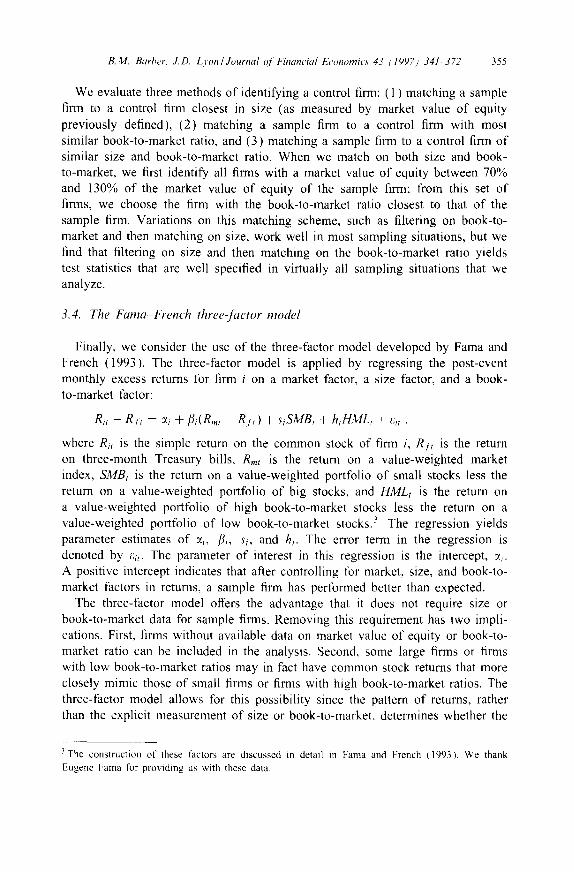
3.4. T h e F a m a F r e n c h t h r e e - [ a c t o r m o d e l

Finally, we consider the use of the three-factor model developed by Fama and French (1993). The three-factor model is applied by regressing the post-event monthly excess returns for firm i on a market factor, a size factor, and a book- to-market factor:

Rit - R t t = :~i + fli( Rml R /t ) + s i S M B t + h i H M L I + r~il ,

where Rit is the simple return on the common stock of finn i, R/t is the return on three-month Treasury bills, Rmt is the return on a value-weighted market index, S M B I is the return on a value-weighted portfolio of small stocks less the return on a value-weighted portfolio of big stocks, and H M L t is the return on a value-weighted portfolio of high book-to-market stocks less the return on a value-weighted portfolio of low book-to-market stocks. 3 The regression yields parameter estimates of :~, [~i, si , and hi. The error term in the regression is denoted by ~:#. The parameter of interest in this regression is the intercept, z~,. A positive intercept indicates that after controlling for market, size, and book-to- market factors in returns, a sample firm has performed better than expected.

The three-factor model offers the advantage that it does not require size or book-to-market data for sample firms. Removing this requirement has two impli- cations. First, firms without available data on market value of equity or book-to- market ratio can be included in the analysis. Second, some large firms or firms with low book-to-market ratios may in fact have common stock returns that more closely mimic those of small firms or firms with high book-to-market ratios. The three-factor model allows for this possibility since the pattern o f returns, rather than the explicit measurement of size or book-to-market, determines whether the

3 The construction of these factors are discussed in detail in Fama and French (1993). We thank Eugene Fama for providing us with these data.

356 B.M. Barber, J.D. Lyon~Journal ~[ Financial Economics 43 (1997) 341 372

returns on a f i rm's c o m m o n stock more closely mimic the returns o f small firms

and /or high book- to-marke t firms.

The three-factor model has two disadvantages. First, g iven four parameters in

the regression, it requires at least five observat ions o f month ly returns post-event .

This creates a survivor bias among remaining sample firms. 4 Second, when long-

hor izon returns (say f ive-year returns) are considered, the regress ion est imates are

assumed stable over the es t imat ion period. Thus, in contrast to the s ize /book- to-

market portfolios, in which a f i rm 's portfol io ass ignment is a l lowed to change

once per year, the regress ion approach assumes that a f i rm's market, size, and

book- to-marke t characterist ics are stable over time. 5

3.5. Survivor~selection biases in Compustat data

Kothari, Shanken, and Sloan (1995) argue that survivor biases in Compus-

tat data may part ial ly explain the relation be tween book- to-marke t ratios and

security returns. They argue that there are two sources o f bias. First, prior to

1978, Compusta t rout inely included historical financial informat ion o f firms. Sec-

ond, Compusta t may back-fil l the financial informat ion o f firms that delayed the

reporting o f their financial s tatements for reasons related to financial distress. The

problem with this type o f back-fi l l ing is that the firms that emerge f rom financial

distress are more l ikely to be back-fil led. However , the accumula t ing evidence

suggests that there is a posi t ive relation be tween book- to-marke t ratios and secu-

rity returns (e.g., Davis, 1994; Chan, Jegadeesh, and Lakonishok, 1995; Barber

and Lyon, 1996b). Furthermore, Chan, Jegadeesh, and Lakonishok (1995) argue

that the survivor bias in Compusta t data is small.

In this research, we are forced to either ignore the possible relat ion be tween

book- to-marke t ratios and security returns or use data that we know are subject

to some survivor bias ( though the extent o f the bias is contested). We choose

to include book- to-marke t ratios in our analysis for four reasons. First, in event

4 It is not clear, ex ante, what effect this survivor bias has on tests for long-run abnormal returns. The direction of the bias depends on the returns of firms in the months immediately prior to delisting. In the case of a merger, acquisition, or going private transaction these returns are likely positive, while in the case of a bankruptcy or liquidation these returns are likely negative.

5 An alternative application of the Fama French three-factor model that we considered, which is analogous to a traditional market model approach, is to estimate three coefficients on the market risk premium, size factor, and book-to-market factor using a pre-event window. Expected returns can be calculated using the estimated coefficients, the risk-free rate, and the realized market, size, and book-to-market risk premiums. Post-event abnormal returns can be calculated using a sample firm's realized return less an expected return. We abandoned this approach for two reasons. First, it requires pre-event return data - a requirement that is not necessary for the reference, control, or Fama French methods that we consider. Second, the estimated coefficients on size and book-to-market are not stable over time, so that applying coefficient estimates from a pre-event estimation window introduces noise into an analysis of long-run abnormal stock returns.

B.M. Barber. J.D. Lyon/Journal o f Financial Economics 43 (1997) 341 372 357

studies over long horizons, the survivor bias will lead to biases in results only if sample firms are more or less likely to have been back-filled by Compustat than the general population. A survivor bias in Compustat data is not sufficient to reject results that document significant long-horizon abnormal returns. Second, the book- to-market and size/book-to-market reference portfolio and control firm approaches should control well for the survivor biases in Compustat data. If book-to-market ratios are an instrument for survivor bias in Compustat data, we can control for the survivor bias inherent in Compustat data by matching sample firms to firms of similar book-to-market ratios. Third, we have reestimated all of our results in the 1979 through 1994 subperiod. Kothari, Shanken, and Sloan (1995) indicate that Compustat did not include historical financial information for firms in its database during this period, though the survivor bias from delayed financial reports persists. The general tenor of our results is similar during this subperiod. Fourth, we have reestimated our results by drawing samples from the population of firms described in Table 2, but without regard to the availability of book-to-market ratios. The results that employ size decile portfolios, size-matched control firms, the Fama French three-factor model, and the equally weighted market index are similar to those that we report later. Barber and Lyon (1996a) thoroughly discuss the impact of dropping the requirements for size and book-to-market data.

4. Statistical tests for long-run abnormal stock returns

We evaluate the empirical specification and power of test statistics based on both CARs (see Eq. (1)) and BHARs (see Eq. (2)) at one-, three-, and five-year horizons. We use the return on either a reference portfolio or a control firm as the expected return for each sample firm when calculating a CAR or BttAR.

It is common for some sample firms to delist their common stock post-event. For example, delisting can result from acquisition, bankruptcy, or going private. When a sample firm is missing return data post-event, we use the return on the corresponding reference portfolio as the realized return. In a random sample of 50,000 firms, we are forced to fill returns in at least one month out of 12 for 4,104 of these firms (8.2%). Of these 4,104 firms, 1,138 are filled in just one month. Of the 600,000 firm-month returns (50,000 times 12 months), we fill 20,889 (3.5%) of the firm-month returns. When a control firm is missing return data post-event, we fill the control firm's return with the corresponding reference portfolio. For example, when sample firms are matched to control firms on size, we fill missing return data for control firms with the return on their corresponding size decile portfolio.

Our results are robust to truncating, rather than filling, the returns of sample firms. However, the sample mean long-run abnormal return calculated with trun- cation does not represent the average return an investor could earn from investing in an executable trading strategy, since the investor's use of the proceeds from

358 B.M. Barber, J.D. Lyon/Journal of Financial Economics 43 (1997) 341~72

an investment in a delisted firm is left unresolved. With filling, it is assumed that investors roll their investment from the delisted firm into a reference portfolio. For this reason, we choose to report results with filling rather than truncation.

We consider the use of four reference portfolios (size deciles, book-to-market deciles, 50 size/book-to-market portfolios, and an equally weighted NYSE/ASE/ NASDAQ market index) and three methods of identifying a control firm (size- matched, book-to-market matched, and size/book-to-market matched). When ref- erence portolios are employed, if the portfolio assignment of a sample firm changes during the event year (say from size decile 10 to 9), the corresponding reference portfolio is also changed. When the control firm methods are used, the same control firm is used throughout the horizon of analysis.

4.1. The statistical tests

To test the null hypothesis that the mean cumulative or buy-and-hold abnormal returns are equal to zero for a sample of n firms, we employ one of two parametric test statistics:

teAR = CARi~/( a( CARiz )/ xfn ) (4)

OF

tBttAR = BHARi~/( a( BHARi~ )/ x/n ) , (5)

where CARn and BHARir are the sample averages and a(CARiz) and a(BHARi~) are the cross-sectional sample standard deviations of abnormal returns for the sample of n firms. If the sample is drawn randomly from a normal distribution, these test statistics follow a Student's t-distribution under the null hypothesis. While the CARs and BHARs are clearly nonnormal, the Central Limit Theo- rem guarantees that if the measures of abnormal returns in the cross-section of firms are independent and identically distributed drawings from finite variance distributions, the distribution of the mean abnormal return measure converges to normality as the number of firms in the sample increases.

We also consider, but abandon, the use of time-series standard deviations to calculate test statistics for CARs. We prefer the use of cross-sectional standard errors because requiring pre-event return data from which a time-series standard error can be estimated exacerbates the new listing bias. In addition, time-series standard deviations cannot be used to calculate a test statistic for BHARs. This issue is discussed in detail by Barber and Lyon (1996a).

4.2. The Fama-French three-factor model

Finally, we consider the application of the Fama-French three-factor model. For a sample of n firms, we estimate n regressions (one for each sample firm).

B.M. Barber, J.D Lyon~Journal ~f Financial Economics 43 ~1997) 341 372 359

The intercept terms from these regressions (:~s) are then averaged across the n sample firms. A parametric t-statistic is calculated by dividing the mean inter- cept term by the cross-sectional sample standard deviation of the intercept terms and mulitplying by the square root of n. The mean intercept term is used to test the null hypothesis that the mean monthly abnormal return of sample firms is equal to zero. Thus, this application of the Fama-French three-factor model is conceptually equivalent to the tests based on cumulative abnormal returns.

4.3. Simulation method

To test the specification of the test statistics based on each of the four refer- ence portfolios, the three control firm methods, and the three-factor model, 1,000 random samples of n event months are drawn without replacement. (Our results are robust to sampling with replacement.) Since our unit of observation is an event month, we are more likely to sample firms with a longer history of return data. We believe that this is sensible, since most event studies analyze events that are proportional to the history of a firm. For example, firms with longer histories will have more equity or debt issues. For each of the 1,000 random samples, the test statistics are computed as described above and compared to the critical value of the test statistic associated with the two-tailed ~ significance level. Sam- pling first by firm and then by event month, which is how Kothari and Warner (1996) conduct their simulations, exacerbates the negative bias of test statistics documented in Section 5: the details of this analysis are discussed in Barber and Lyon (1996a).

If a test is well specified, 1,000~ tests will reject the null hypothesis of zero mean abnormal returns. A test is conservative if fewer than 1,000:~ null hy- potheses are rejected, while a test is anticonservative if more than 1,000e null hypotheses are rejected. Based on this procedure, we test the specification of each test statistic at the 1%, 5%, and 10% theoretical levels of significance. A well- specified two-tailed test of the null hypothesis of zero mean abnormal returns will reject the null at the theoretical rejection level in favor of the alternative hy- pothesis of negative (positive) abnormal returns in 1,000~/2 samples. Thus, we separately document rejections of the null hypothesis in favor of the alternative hypothesis that long-run abnormal returns are positive or negative. For example, at the 1% theoretical significance level, we document the percentage of calcu- lated t-statistics that are less than the theoretical cumulative density function of the t-statistic at 0.5% and greater than the theoretical cumulative density function at 99.5%. Finally, to evaluate the impact of the new listing, rebalancing, and skewness biases, we also compute the mean and skewness for abnormal returns across all 1,000 samples times n observations for each simulation.

In sum, we calculate the empirical specification of test statistics based on (1) 15 methods of calculating abnormal returns (CARs using the four reference

360 B.M. Barber, J.D. Lyon~Journal of Financial Economics 43 (1997) 341 372

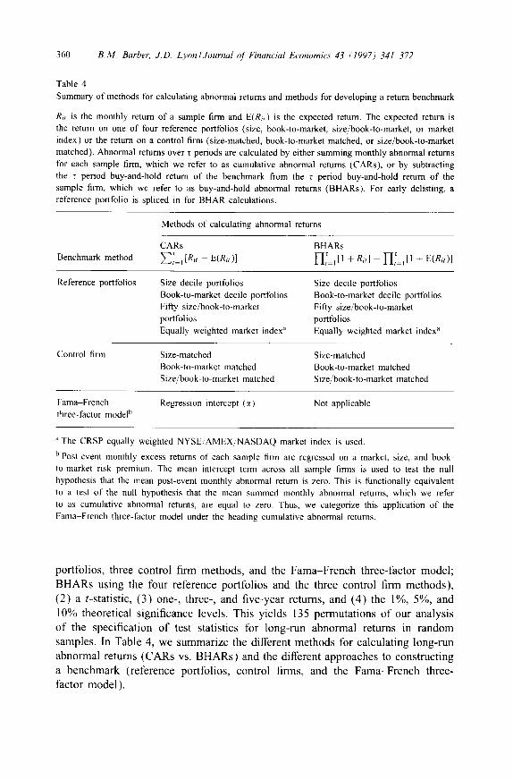
Table 4 Summary of methods for calculating abnormal returns and methods for developing a return benchmark

Rit is the monthly return of a sample firm and E(Rit) is the expected return. The expected return is the return on one of four reference portfolios (size, book-to-market, size/book-to-market, or market index) or the return on a control firm (size-matched, book-to-market matched, or size/book-to-market matched). Abnormal returns over z periods are calculated by either summing monthly abnormal returns for each sample firm, which we refer to as cumulative abnormal returns (CARs), or by subtracting the z period buy-and-hold return of the benchmark from the r period buy-and-hold return of the sample firm, which we refer to as buy-and-hold abnormal returns (BHARs). For early delisting, a reference portfolio is spliced in for BHAR calculations.

Benchmark method

Methods of calculating abnormal returns

CARs BHARs

1- IZ Il + R.I - H =,rl E R,,)1

Reference portfolios Size decile portfolios Book-to-market decile portfolios Fifty size/book-to-market portfolios Equally weighted market index a

Size decile portfolios Book-to-market decile portfblios Fifty size/book-to-market portfolios Equally weighted market index a

Control firm Size-matched Book-to-market matched Size/'book-to-market matched

Size-matched Book-to-market matched Size/'book-to-market matched

Fama French Regression intercept (:~) Not applicable three-factor model b

a The CRSP equally weighted NYSE/AMEX/NASDAQ market index is used.

b Post-event monthly excess returns of each sample firm are regressed on a market, size, and book- to-market risk premium. The mean intercept term across all sample finns is used to test the null hypothesis that the mean post-event monthly abnormal return is zero. This is functionally equivalent to a test of the null hypothesis that the mean summed monthly abnormal returns, which we refer to as cumulative abnormal returns, are equal to zero. Thus, we categorize this application of the Fama French three-factor model under the heading cumulative abnormal returns.

p o r t f o l i o s , t h r ee c o n t r o l f i rm m e t h o d s , a n d the F a m ~ F r e n c h t h r e e - f a c t o r m o d e l ;

B H A R s u s i n g the fou r r e f e r e n c e p o r t f o l i o s a n d the t h r e e c o n t r o l f i rm m e t h o d s ) ,

( 2 ) a t - s ta t i s t i c , ( 3 ) one - , t h r ee - , a n d f i v e - y e a r re tu rns , a n d ( 4 ) the 1%, 5 % , a n d

10% t h e o r e t i c a l s i g n i f i c a n c e leve ls . Th i s y i e ld s 135 p e r m u t a t i o n s o f ou r a n a l y s i s

o f t he s p e c i f i c a t i o n o f tes t s ta t i s t ics for l o n g - r u n a b n o r m a l r e tu rns in r a n d o m

s a m p l e s . In Tab le 4, w e s u m m a r i z e t he d i f f e ren t m e t h o d s fo r c a l c u l a t i n g l o n g - r u n

a b n o r m a l r e t u r n s ( C A R s vs. B H A R s ) a n d the d i f f e ren t a p p r o a c h e s to c o n s t r u c t i n g

a b e n c h m a r k ( r e f e r e n c e p o r t f o l i o s , con t ro l f i rms , and the F a m a - F r e n c h th ree -

f ac to r m o d e l ) .

B.M. Barber. J.D. Lyon~Journal o/Financial Economics 43 (1997) 341 372 361

5. Results

In this section, we document the specification and power of t-statistics using long-run CARs and BHARs. We begin with a discussion of the results in random samples, followed by a discussion of results in samples with size-based and book-to-market based sampling biases. We close this section with a discussion of measurement bias associated with the use of CARs. In discussing our results, we liberally refer to the new listing, skewness, and rebalancing biases outlined in detail in Section 2.

5. 1. Random samples

5.1.1. Cumulative abnormal returns The first set of results is based on 1,000 random samples of 200 event months

drawn from our population of over 1.1 million possible event months. The specification of t-statistics using 12-month, 36-month, and 60-month CARs and the Fama-French three-factor model is presented in Table 5. Recall that these t-statistics test the null hypothesis that the mean monthly abnormal return during the event period is zero.

Three results are noteworthy. First, cumulative abnormal returns calculated us- ing reference portfolios yield test statistics that are positively biased. The mag- nitude of the bias increases with the horizon of cumulation. This positive bias can be attributed to the positive mean abnormal return, which results from the new listing bias. Note that this positive bias is most pronounced when an equally weighted market index is used to calculate the CARs. This result can be traced to the fact that firms included in the size, book-to-market, and size/book-to-market reference portfolios must have prior period data on size and book-to-market ratios. This requirement for prior-period data for firms constituting the index mitigates (but does not eliminate) the new listing bias.

Second, all of the control firm approaches yield well-specified test statistics. (The one exception is the size-matched control firm approach at the 5% signifi- cance level and 36 months. We suspect random sampling variation accounts for this result.) Note that when the control firm approaches are employed at 36- and 60-month horizons, the resulting mean CAR is more closely centered on zero than is the mean CAR calculated using reference portfolios. The control firm approach effectively eliminates the new listing bias.

Third, the Fama French three-factor model yields negatively biased test statis- tics at 12- and 36-month horizons. Fama and French (1993, Table 9a) docu- ment that portfolios of small firms yield negative intercepts when regressed on their three factors. Similarly, when we regress the monthly return on the CRSP equally weighted market index less the return on Treasury bills on the Fama- French factors from July 1963 to December 1994 the resulting intercept term is -0 .08%. Recall that event studies give equal weight to sample observations,

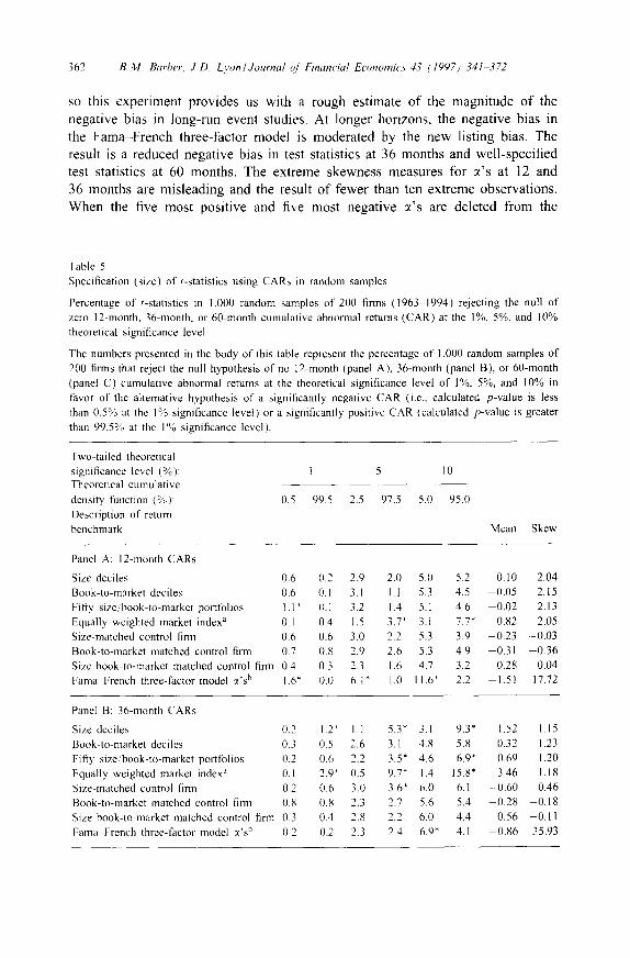
362 B.M. Barber, J.D. Lyon~Journal o! Financial Economics 43 (1997) 341 372

SO th is e x p e r i m e n t p r o v i d e s us w i th a r o u g h e s t i m a t e o f t he m a g n i t u d e o f t he

n e g a t i v e b ias in l o n g - r u n e v e n t s tud ies . A t l o n g e r h o r i z o n s , t he n e g a t i v e b i a s in

t he F a m a - F r e n c h t h r e e - f a c t o r m o d e l is m o d e r a t e d by the n e w l i s t ing bias . T h e

resu l t is a r e d u c e d n e g a t i v e b i a s in tes t s ta t i s t i cs at 36 m o n t h s and w e l l - s p e c i f i e d

tes t s ta t i s t ics at 60 m o n t h s . T h e e x t r e m e s k e w n e s s m e a s u r e s for :~'s at 12 a n d

36 m o n t h s are m i s l e a d i n g a n d the resu l t o f f e w e r t han t e n e x t r e m e o b s e r v a t i o n s .

W h e n the f ive m o s t p o s i t i v e and five m o s t n e g a t i v e ~ ' s a re d e l e t e d f r o m the

Table 5 Specification (size) of t-statistics using CARs in random samples

Percentage of t-statistics in 1,000 random samples of 200 firms (1963 1994) rejecting the null of zero 12-month, 36-month, or 60-month cumulative abnormal returns (CAR) at the 1%, 5%, and 10% theoretical significance level

The numbers presented in the body of this table represent the percentage of 1,000 random samples of 200 firms that reject the null hypothesis of no 12-month (panel A), 36-month (panel B), or 60-month (panel C) cumulative abnormal returns at the theoretical significance level of 1%, 5%, and 10% in favor of the alternative hypothesis of a significantly negative CAR (i.e.. calculated p-value is less than 0.5% at the 1% significance level) or a significantly positive CAR (calculated p-value is greater than 99.5% at the I% significance level).

Two-tailed theoretical significance level (%): Theoretical cumulative density function (%): Description of return benchmark

1 5 I0

0.5 99.5 2.5 97.5 5.0 95.0

Mean Skew

Panel A: 12-month CARs

Size deciles 0.6 0.2 2.9 Book-to-market deciles 0.6 0.1 3.1 Fifty size/book-to-market porttblios 1.1 * 0.1 3.2 Equally weighted market index a 0.1 0.4 1.5 Size-matched control firm ll.6 0.6 3.0 Book-to-market matched control finn 0.7 0.8 2.9

0.3 2.3 0.0 6.1"

Size book-to-market matched control finn 0.4 Fama French three-factor model ~'s b 1.6"

2.0 5.0 5.2 0.10 2.04 1.1 5.3 4.5 0.05 2.15 1.4 5.1 4.6 0.02 2.13 3.7* 3.1 7.7* 0.82 2.05 2.2 5.3 3.9 -0.23 -0.03 2.6 5.3 4.9 -0.31 0.36 1.6 4.7 3.2 -0.28 0.04 1.0 11.6" 2.2 1.51 17.72

Panel B: 36-month CARs

Size deciles 0.2 1.2" 1.1 5.3* 3.1 9.3* 1.52 1.15 Book-to-market deciles 0.3 0.5 2.6 3.1 4.8 5.8 0.32 1.23 Fifty size/book-to-market portfolios 0.2 0.6 2.2 3.5* 4.6 6.9* 0.69 1.20 Equally weighted market index a 0.1 2.9* 0.5 9.7* 1.4 15.8" 3.46 1.18 Size-matched control finn 0.2 0.6 3.0 3.6* 6.0 6.1 -0.60 0.46 Book-to-market matched control finn 0.8 0.8 2.3 2.7 5.6 5.4 0.28 0.18 Size book-to-market matched control finn 0.3 0.4 2.8 2.2 6.0 4.4 0.56 -0.11 Farna French three-factor model z~'s b 0.2 0.2 2.3 2.4 6.9 ~ 4.1 -0 .86 35.93

B.M. Barber, J.D. Lyon/Journal ()f Financial Economics 43 (1997; 341 372

Table 5 (continued)

363

Two-tailed theoretical

significance level (%): Theoretical cumulative

density function (%):

Description of return

benchmark

1 5 l0

0.5 99.5 2.5 97.5 5.0 95.0

Mean Skew

Panel C: 60-month CARs

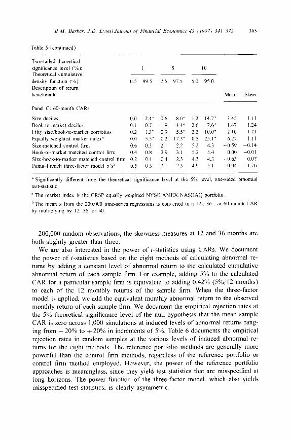
Size deciles 0.0 2A* 0.6 8.0* 1.2 14.7" 3.45 1.11

Book-to-market deciles 0.1 0.7 1.9 4.4* 2.6 7.6* 1.47 1.24

Fifty size/book-to-market portfolios 0.2 1.3 * 0.9 5.5* 2.2 10.0" 2.10 1.21

Equally weighted market index a 0.0 5.5" 0.2 17.3" 0.5 25.1 * 6.27 1.11

Size-matched control firm 0.6 0.3 2.1 2.2 5.2 4.3 -0 .59 -0 .14

Book-to-market matched control firm 0.4 0.8 2.9 3.1 5.2 5.4 0.00 -0.01 0.4 2.4 2.3 4.3 4.3 -0 .63 0.07 0.3 2.1 2.3 4.9 5.1 -0 .94 -1 .76

Size/book-to-market matched control firm 0.2 Fama-French three-factor model 7's b 0.5

* Significantly different from the theoretical significance level at the 5% level, one-sided binomial

test-statistic.

a The market index is the CRSP equally weighted NYSE/AMEX/NASDAQ portfolio.

b The mean :c from the 200,000 time-series regressions is converted to a 12-, 36-, or 60-month CAR

by multiplying by 12, 36, or 60.

200,000 random observations, the skewness measures at 12 and 36 months are both slightly greater than three.

We are also interested in the power of t-statistics using CARs. We document the power of t-statistics based on the eight methods of calculating abnormal re- turns by adding a constant level of abnormal return to the calculated cumulative abnormal return of each sample firm. For example, adding 5% to the calculated CAR for a particular sample firm is equivalent to adding 0.42% (5%/12 months) to each of the 12 monthly returns of the sample firm. When the three-factor model is applied, we add the equivalent monthly abnormal return to the observed monthly return of each sample firm. We document the empirical rejection rates at the 5% theoretical significance level of the null hypothesis that the mean sample CAR is zero across 1,000 simulations at induced levels of abnormal returns rang- ing from - 20% to - 20% in increments of 5%. Table 6 documents the empirical rejection rates in random samples at the various levels of induced abnormal re- turns for the eight methods. The reference portfolio methods are generally more powerful than the control firm methods, regardless of the reference portfolio or control firm method employed. However, the power of the reference portfolio approaches is meaningless, since they yield test statistics that are misspecified at long horizons. The power function of the three-factor model, which also yields misspecified test statistics, is clearly asymmetric.

364 B. M Barber, J.D. Lyon / Journal Of Financial Economics 43 (1997) 341 372

Table 6 Power of t-statistics using 12-month CARs in random samples

Percentage of 1,000 random samples of 200 firms (1963 1994) with induced abnormal returns ranging from -20% to ~20% rejecting the null hypothesis of zero 12-month cumulative abnormal return (CAR) at 5% theoretical significance level

The numbers presented in the body of this table represent the percentage of 1,000 random samples that reject the null hypothesis of no abnormal returns at the theoretical significance level of 5% and various levels of induced abnormal returns. Abnormal returns are induced by adding a constant to the observed cumulative abnormal return for each of the 200 randomly selected firms in all 1,000 random samples. Thus, for example, adding 5% to the 12-month CAR is equivalent to a 0.42% monthly abnormal return.

Induced level of abnormal return (%):

Description of return benchmark

-20 -15 10 - 5 0 5 10 15 20

Size deciles 99 98 82 35 5 32 87 100 100 Book-to-market deciles 99 98 84 36 4 30 86 100 100 Fifty size/book-to-market portfolios 99 98 84 36 5 32 87 100 100 t Equally weighted NYSE/AMEX NASDAQ index 99 97 76 25 5 39 91 100 100 t Size-matched control firm 98 89 59 19 5 17 56 86 98 Book-to-market matched control finn 98 88 58 21 6 17 54 86 97 Size,book-to-market matched control firm 98 89 60 20 4 15 56 87 98 Fama- French three-factor model ~'s 96 88 66 28 7 9 32 66 87 t

t Empirical tests based on this statistic are anticonser,,ative at the 1%, 5%. and/or 10% theoretical significance level (see Table 5).

5.1.2. Buy-and-hold abnormal returns The specification of t-statistics using long-run buy-and-hold returns is presented

in Table 7. Recall that these test statistics test the null hypothesis that the annual abnormal return is zero. We highlight two results o f this analysis. First, there is a significant negative bias in t-statistics based on abnormal returns calculated using the four reference portfolios. The negative bias can ultimately be traced to the rebalancing and skewness biases. Though the new listing bias generally leads to positive mean CARs (particularly at long horizons), the rebalancing bias more than offsets the new listing bias when BHARs are calculated using a reference portfolio. The result is a negative mean BHAR. The one exception to this result is at five years when the equally weighted index is used. (Recall that the use o f size, book-to-market, and size/book-to-market reference portfolios mitigates the new listing bias due to the requirement that firms included in a reference portfolio have prior-period data.)

The skewness bias also exacerbates the negative bias in test statistics. Note that the skewness o f BHARs is much more pronounced than that o f CARs. The ef- fect o f skewness on test statistics is best revealed on close inspection o f five-year

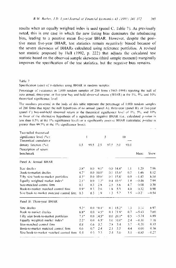
B.M. Barber, J.D. Lyon~Journal o/Financial Economi~s 43 "1997~ 341 372 365

results when an equally weighted index is used (panel C, Table 7). As previously noted, this is one case in which the new listing bias dominates the rebalancing bias, leading to a positive mean five-year BHAR. However, despite the posi- tive mean five-year BHAR, test statistics remain neqatively biased because of the severe skewness of BHARs calculated using reference portfolios. A revised test statistic proposed by Hall (1992, p. 222) that adjusts the calculated test statistic based on the observed sample skewness (third sample moment) marginally improves the specification of the test statistics, but the negative bias remains.

Table 7

Specification (size) of t-statistics using BHAR in random samples

Percentage of t-statistics in 1,000 random samples of 200 finns I1963 1994) rejecting the null of zero annual, three-year, or five-year buy-and-hold abnormal returns (BHAR) at the I%, 5%, and 10%

theoretical significance level

The numbers presented in the body of this table represent the percentage of 1.000 random samples

of 200 firms that reject the null hypothesis of no annual (panel A), three-year (panel B), or five-year

(panel C) buy-and-hold abnormal return at the theoretical significance level of 1%, 5%, and 10% in favor of the alternative hypothesis of a significantly negative BHAR (i.e.. calculated p-value is

less than 0.5% at the 1% significance level) or a significantly positive BHAR (calculated p-value is

greater than 99.5% at the 1% significance level).

Two-tailed theoretical

significance level (%): Theoretical cumulative

density function (%):

Description of return

benchmark

I 5 10

0.5 99.5 2.5 97.5 5.0 95.0

Mean Skew

Panel A: Annual BHAR

Size deciles 3.8 ~ 0.0 9.1" 0.0 14.4" 1.1 1.20 7.96

Book-to-market deciles 4.7 ~ 0.0 10.0" 0.1 15.6" 0.7 - I . 4 6 8.12 Fifty size,book-to-market porttblios 4.3 * 0.0 10.0" 0.1 15.8" 0.9 1.43 8.10

Equally weighted market index a 2.1" 0.0 7.3* (1.4 10.5" 1.9 0.48 7.99 Size-matched control [inn 0.1 0.3 2.8 2.5 5.6 4.7 -0 .08 0.38

Book-to-market matched control finn 0.9" 0.3 2.6 1.8 5.3 4.0 0.32 0.98

0.3 1.9 13 5.2 3.5 0.21 0.54 Size:book-to-market matched control firm 0.3

Panel B: Three-year BHAR

Size decilcs 5.2* 0.0 10.4 ~ /).l 15.2" 1.3 -3.14 6.97

Book-to-market deciles 6.8* 0.0 14.5" 0.1 21.9" 0.7 5.43 7.00

Fifty size, book-to-market portfolios 7.1" 0.0 14.5" 0.0 2(/.I ~ 0,5 -5 .24 6.89

Equally weighted market index ~ 2.2* 0.0 6.5* 1.0 10.0 ~ 2.4 -0 .10 7.16

Size-matched control finn 0.8 0.6 3.2 2.8 5.4 5.7 0.20 0.33 Book-to-market matched control firm 0.6 0.7 2.4 2.1 5.5 4.4 0.00 0.36

0.3 2.3 2.4 5.0 5.1 0.85 0.27 Size/book-to-market malched control firm 0.4

366 BM. Barber, J.D. Lyon/Journal qIFinancial Economics 43 ,/1997)341 372

Table 7 (continued)

Two-tailed theoretical significance level (%): Theoretical cumulative density function (%): Description of return benchmark

I 5 10

(1.5 99.5 2.5 97.5 5.0 95.0

Mean Skew

Panel C: Five-year BHAR

Size deciles 4.2* 0.0 9.8* 0.6 15.7" 1.0 -4.86 12.48 Book-to-market deciles 7.8* 0.0 15.8" 0.1 23.1" 0.3 9.62 12.35 Fifty size/book-to-market portfolios 7.2 ~ 0.0 16.3" 0.2 23.1" 0.7 9.67 12.19 Equally weighted market index a 1.6" 0.1 4.4 ~ 0.7 7.7* 2.5 2.00 12.66 Size-matched control firm 0.6 0.4 3. I 2.6 5.3 5. I 0.08 1.51 Book-to-market matched control firm 0.3 0.4 2.0 2.2 4.0 4.8 1.46 2.55

0.1 2.5 2.4 5.0 3.9 1.12 1.61 Size.book-to-market matched control firm 0.3

Significantly different from the theoretical significance level at the 5% level, one-sided binomial test-statistic.

The market index is the CRSP equally weighted NYSE"AMEX/NASDAQ portfolio.

The second noteworthy result is the efficacy of the control firm approach. When the control firm approaches are employed, the mean BHAR and skew- ness are generally both much closer to zero than when the reference portfolio

approach is used. As argued previously, the control firm approach alleviates the new listing, rebalancing, and skewness biases that plague BHARs calculated us-

ing reference portfolios. Thus, test statistics based on the control finn approach are well specified. (The one exception is the book-to-market matched control firm

approach at the 1% significance level and an annual horizon. We suspect random sampling variation accounts for this result.)

As was done for CARs, we analyze the empirical power of the various test statistics by adding a constant level of abnormal return to the calculated an- nual BHAR of each sample firm. However, with buy-and-hold abnormal returns, adding 5% to the annual BHAR does not correspond to a particular pattern of monthly abnormal returns. Thus, direct comparisons of the power of t-statistics using CARs (presented in Table 6) and BHARs (presented in Table 8) are not

meaningful. Table 8 documents the empirical rejection rates in random samples at the various levels of induced abnormal returns for the seven methods. Two observations emerge from this analysis. First, the reference portfolio methods of

calculating annual buy-and-hold abnormal returns yield asymmetric power func- tions. Second, though symmetric, the control firm methods are less powerful than the reference portfolio methods. Nonetheless, we cannot recommend the use of the reference portfolio methods because they yield severely misspecified test statistics.

B.M. Barber. J.D. Lyon~Journal o] Financial Economics 43 (I997) 341 372 367

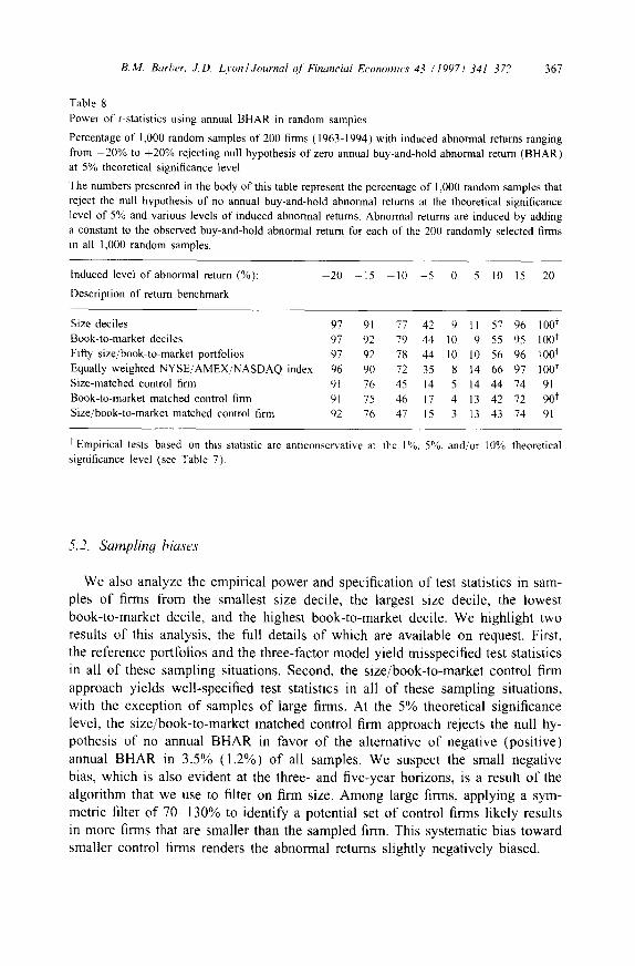
Table 8 Power of t-statistics using annual BHAR in random samples

Percentage of 1,000 random samples of 200 firms (1963-1994) with induced abnormal returns ranging from -20% to +20% rejecting null hypothesis of zero annual buy-and-hold abnormal return (BHAR) at 5% theoretical significance level

The numbers presented in the body of this table represent the percentage of 1,000 random samples that reject the null hypothesis of no annual buy-and-hold abnormal returns at the theoretical significance level of 5% and various levels of induced abnormal returns, Abnormal returns are induced by adding a constant to the observed buy-and-hold abnormal return for each of the 200 randomly selected finns in all 1,000 random samples.

Induced level of abnormal return (%): -20 -15 10 - 5 0 5 10 15 20

Description of return benchmark

Size deciles 97 91 77 42 9 11 57 96 100 t Book-to-market deciles 97 92 79 44 10 9 55 95 100 t Fifty size/book-to-market portfolios 97 92 78 44 10 10 56 96 1001 Equally weighted NYSE/AMEX/NASDAQ index 96 90 72 35 8 14 66 97 100 t Size-matched control firm 91 76 45 14 5 14 44 74 91 Book-to-market matched control firm 91 75 46 17 4 13 42 72 90 t Size/book-to-market matched control firm 92 76 47 15 3 13 43 74 91

t Empirical tests based on this statistic are anticonservative at the I%, 5%, and/or 10% theoretical significance level (see Table 7).

5.2. Sampl ing biases

We also analyze the empir ical power and specif icat ion o f test statistics in sam-

ples o f firms from the smallest size decile, the largest size decile, the lowest

book- to-marke t decile, and the highest book- to-market decile. We highl ight two

results o f this analysis, the full details o f which are avai lable on request. First,

the reference portfol ios and the three-factor model yield misspecif ied test statistics

in all o f these sampl ing situations. Second, the s ize /book- to-marke t control f inn

approach yields wel l -specif ied test statistics in all o f these sampl ing situations,

with the except ion o f samples o f large finns. At the 5% theoret ical s ignificance

level, the s ize /book- to-marke t matched control firm approach rejects the null hy-

pothesis o f no annual B H A R in favor o f the al ternative o f negat ive (posi t ive)

annual B H A R in 3 .5% (1 .2%) o f all samples. We suspect the small negat ive

bias, which is also evident at the three- and f ive-year horizons, is a result o f the

a lgor i thm that we use to filter on firm size. A m o n g large finns, applying a sym-

metric filter o f 7 0 - 1 3 0 % to identify a potential set o f control firms likely results

in more firms that are smaller than the sampled finn. This systematic bias toward

smaller control firms renders the abnormal returns sl ightly negat ive ly biased.

368 B.M. Barber. J.D. Lyon/Journal o! Financial Economics 43 (1997) 341 372

5.3. Measurement bias

Recall that conceptually we favor the use of buy-and-hold abnormal returns for two reasons. First, they measure the underlying parameter of interest, which is the long-run performance of the common stock of sample firms relative to an appropriate comparison group. For example, a mean annual BHAR of 5% can be interpreted as the additional return earned from investing in a sample firm relative to a control firm over the year. In contrast, a 12-month CAR of 5% does not readily translate into a measure of annual performance. The second reason that we favor the use of BHARs is that CARs are a biased predictor of BHARs (see Section 2).

To assess the extent of the measurement bias, we conduct the following ex- periment, in each of our simulations, we analyze the CARs and BHARs for the same sets of 1,000 samples. In each of the 1,000 samples at the 5% theoretical significance level, we determine in what proportion of these samples a researcher would draw different inferences based on BHARs and CARs. For example, if at the 5% theoretical significance level a researcher would reject the null hypothe- sis of no abnormal returns when BHARs are employed, but fails to reject when CARs are employed, we would characterize this as a different inference based on BHARs and CARs. In this experiment, we use the size/book-to-market con- trol firm approach, since this method yields well-specified test statistics for both CARs and BHARs in most sampling situations. (It is not useful to compare the inferences drawn from CARs and BHARs calculated using reference portfolios, since CARs and BHARs are differentially affected by the new listing, rebalancing, and skewness biases.)

Based on this analysis, we find that a researcher would obtain different infer- ences in 3.7% of 1~000 randomly selected samples of 200 observations. Among samples of small firms, this figure increases to 4.7%.

6. Tests of median return performance

We also consider a nonparametric Wilcoxon signed-rank test statistic. We use the large-sample approximation for the Wilcoxon signed-rank test statistic de- scribed by Hollander and Wolfe (1973). If rankings are tied, the average ranks are used. The Wilcoxon signed-rank test statistic tests the null hypothesis that the median abnormal return is equal to zero. This may be a particularly useful hypothesis to test when a researcher is concerned with making inferences about the median firm in a particular sample. For example, Ritter (1991) argues that firms that go public do so partially to take advantage of a window of opportunity in which their stock is overvalued. Tests of the null hypothesis that the mean annual BHAR is zero do not allow us to conclude that the median firm is able to take advantage of a window of opportunity, since a negative mean BHAR

B.M. Barber, J.D. Lyon~Journal of Financial Economics 43 (1997) 341 372 369

can be driven by unusually large negative abnormal returns for a few sample firms.

The positive skewness in annual BHARs calculated using reference portfolios renders Wilcoxon signed-rank test statistics hopelessly misspecified (recall that the median BHAR calculated using a market index is - 7%) . For example, when a reference portfolio is used to calculate abnormal returns, the null hypothesis of a zero median annual BHAR is rejected in favor of the alternative hypothesis of a negative median annual BHAR in from 52% to 65% of random samples of size 200 at the 5% theoretical significance level. The positive skewness in 12-month CARs calculated using reference portfolios, though less severe, still yields negatively biased test statistics. At the 5% two-tailed theoretical significance level, the rejections of the null hypothesis in favor of the alternative hypothesis of a negative median annual BHAR range from 3.6% to 7.3%.

In order to obtain a well-specified test of the null hypothesis that the median annual BHAR is zero, a researcher must match sample firms to an appropriate control firm. We find that the size/book-to-market control firm method yields well-specified Wilcoxon test statistics in all sampling situations that we analyze. The results for tests on the median 12-month CAR are similar. As for t-statistics, there is a slight negative bias in the Wilcoxon test statistic among samples of large firms, which we suspect can be traced to our algorithm for matching on firm size.

We also analyze the power of the Wilcoxon test statistic using the same proce- dure previously described. These results (not reported in a table) indicate that it is somewhat easier to detect nonzero median abnormal returns than nonzero mean abnormal returns. With the size/book-to-market matched control firm method, a 10% ( - 1 0 % ) abnormal return added to each of our sampled firms enables us to reject the null hypothesis of a zero median BHAR in 70% (73%) of our 1,000 random samples of 200 firms. The corresponding rejection rates for testing the null hypothesis of a zero mean annual BHAR are 47% and 43% (see Table 8). The results are similar for 12-month CARs.

7. Conclusion

We document the empirical power and specification of test statistics used in event studies designed to detect long-run (one- to five-year) abnormal stock returns. We analyze two main issues in this research. First, we consider the calculation of abnormal returns. Second, we evaluate three general approaches for developing a benchmark for the calculation of long-run abnormal returns, in- cluding: (1) a reference portfolio, (2) an appropriately matched control firm, and (3) an application of the Fama-French three-factor model.

We argue that long-run abnormal returns should be calculated as the long-run buy-and-hold return of a sample firm less the long-run return of an appropriate benchmark, to which we refer as a buy-and-hold abnormal return. We advocate

370 t~ M. Barber, J.D. Lyon~Journal gfFinancial Economics 43 ,1997) 341 372

the use of buy-and-hold abnormal returns over cumulative abnormal returns for two reasons. First, we document that CARs are biased predictors of BHARs. This problem at its worst can lead to incorrect inferences. For example, we doc- ument that a sample of firms that all have zero annual buy-and-hold abnormal returns calculated relative to a market benchmark has a corresponding 12-month mean cumulative abnormal return of + 5%, on average. In this sampling situation, researchers who restrict their analysis to cumulative abnormal returns and ignore the analysis of buy-and-hold abnormal returns could conceivably conclude that the sample in question earned long-run abnormal returns when in fact it did not. In random samples, we document that researchers would draw different infer- ences using CARs in lieu of BHARs in roughly 4% of all sampling situations. Second, even if the inference based on cumulative abnormal returns is correct, the documented magnitude does not correspond to the value of investing in the average or median sample firm relative to an appropriate benchmark over the horizon of interest. Yet this is precisely the objective of long-run event studies of stock returns.

In addition, we document that there are significant biases in test statistics when long-run abnormal returns are calculated using a reference portfolio (such as a market index). We identify three reasons for the bias in test statistics based on abnormal returns calculated in this manner - the new listing bias, the rebalancing bias, and the skewness bias. Cumulative abnormal returns are most affected by the new listing bias. As a result, long-run cumulative abnormal returns and the associated test statistics are generally positively biased. In contrast, long-run buy- and-hold abnormal returns are more affected by the rebalancing and skewness biases. As a result, long-run buy-and-hold abnormal returns and the associated test statistics are generally negatively biased. Though these reference portfolio approaches are the most commonly used methods in financial economics, our results and those of Kothari and Warner (1996) highlight the problems associated with calculating long-run abnormal returns using either a reference portfolio or an asset pricing model.

Finally, and perhaps most importantly, we identify a method of measuring long-run abnormal returns that yields well-specified test statistics. We document that matching sample firms to control firms of similar size and book-to-market ratios yield well-specified test statistics in virtually all sampling situations that we consider. By matching sample firms to control firms on specified firm char- acteristics, we are able to alleviate the new listing bias (since both sample and control firms must be listed in the identified event month), the rebalancing bias (since the returns of the sample and control firms are compounded in an ana- logous fashion), and the skewness bias (since abnormal returns calculated using this control finn approach are reasonably symmetric). Matching on firm size and book-to-market ratio works well in random samples and samples with size-based or book-to-market based sampling biases. However, as future research in financial economics discovers additional variables that explain the cross-sectional variation

B.M. Barber, .I.D. Lyon~Journal of Financial Economies 43 (1997) 341 372 371

in common stock returns, it will also be important to consider these additional variables when matching sample firms to control firms.

References

Agrawal, Anup and Jeffrey F. Jaffe, 1996, The pre-acquisition performance of target firms: A re- examination of the inefficient management hypothesis, Working paper (Wharton School, University of Pennsylvania, Philadelphia, PA).

Agrawal, Anup, Jeffrey F. Jail'e, and Gershon Mandelker, 1992, The post-merger performance of acquiring firms in acquisitions: A re-examination of an anomaly, Journal of Finance 47, 1605 1621.

Asquith, Paul and Lisa Muelbroek, 1996, An empirical investigation of short interest, Working paper (Ha~'ard Business School, Cambridge, MA).

Ball, Ray, S.P. Kothari, and Charles E. Wasley, 1995, Can we implement research on stock trading rules?, Journal of Portfolio Management 21, 54 63.

Barber, Brad M. and John D. Lyon, 1996a, How can long-run abnormal stock returns be both positively and negatively biased?. Working paper (University of California, Davis, CA).

Barber. Brad M. and John D. Lyon, 1996b, Firm size, book-to-market ratio, and security returns: A holdout sample of financial firms, Journal of Finance, forthcoming.

Bernard, Victor and J. Thomas, 1989, Post+earnings-announcement drift: Delayed price response or risk premium?, Journal of Accounting Research, Supplement, 1-36.

Blume. Marshall E. and Robert F. Stambaugh, 1983, Biases in computed returns: An application to the size effect, Journal of Financial Economics 12, 387-404.

Brav, Alon and Paul A. Gompers, 1995, Myth or reality? The long-run underperformance of initial public offerings: Evidence from venture and nonventure capital-backed companies, Working paper (Harvard Business School, Cambridge, MA).

Brav, Alon, Christopher Geczy, and Paul A. Gompers, 1995. The long-run underperformance of seasoned equity offerings revisited, Working paper (Harvard Business School, Cambridge, MA).

Brown, Stephen J. and Peter F. Pope, 1996, Post-earnings announcement drift'?, Working paper (New York University. New York, NY).

Brown, Stephen J. and Jerold B. Warner, 1980, Measuring security price performance, Journal of Financial Economics 8, 205-258.

Brown, Stephen J. and Jerold B. Warner, 1985, Using daily stock returns: The case of event studies, Journal of Financial Economics 14, 205--258.

Campbell, Cynthia J+ and Charles E. Wasley, 1993, Measuring security price performance using daily NASDAQ returns, Journal of Financial Economics 33, 73 92.

Canina, Linda, Roni Michaely, Richard Thaler, and Kent Womack, 1996, A warning about using the daily CRSP equally-weighted index to compute long-run excess returns, Journal of Finance, forthcoming.

Chan, Louis K.C., Narasimhin Jegadeesh, and Josef Lakonishok, 1995, Evaluating the performance of value versus glamour stocks: The impact of selection bias, Journal of Financial Economics 38, 269-296.

Conrad, Jennifer and Gautum Kaul, 1993, Long-term market overreaction or biases in computed returns?, Journal of Finance 48, 39 64.

Davis, James k., 1994, The cross-section of realized stock returns: The pre-Compustat evidence, Journal of Finance 49, 1579 1593.

Desai, Hemang and Prem C. Jain, 1995, An analysis of the recommendations of the "superstar' money managers at Barton's annual roundtable, Journal of Finance 50, 1257 1274.

Desai. Hemang and Prem C. Jain, 1996, Long-run common stock returns following stock splits and stock dividends, Working paper (Tulane University, New Orleans, LA).

372 R M . Barber. J.D. Lyon/Journal ~?/ Financial Economics 43 (1997) 341 372

Dharan. Bala G. and David Ikenberry, 1995, The long-run negative drift of post-listing stock returns, Journal of Finance 50, 1547 1574.

Dimson, Elroy and Paul Marsh, 1986, Event study methodologies and the size effect, Journal of Financial Economics I7, 113 142.

Dyckman. Thomas, Donna Philbrick, Jens Stephan, and William E. Ricks, 1984, A comparison of event study methodologies using daily stock returns: A simulation approach. Journal of Accounting Research 22. 1-33,

Fama. Eugene F. and Kenneth French, 1992, The cross-section of expected stock returns, Journal of Finance 47, 427--466.

Fama. Eugene F. and Kenneth French, 1993. Common risk factors in returns on stocks and bonds, Journal of Financial Economics 33, 3 56.

Field, Laura Casares, 1996, Is institutional investment in initial public offerings related to long-run performance of these firms'?, Working paper (University of California, Los Angeles, CA).

Gompers, Paul and Josh Lerner, I995, Venture capital distributions: short-run and long-run reactions, Working paper (Harvard Business School, Cambridge, MA).

Hall, Peter, 1992, On the removal of skewness by transformation, Journal of the Royal Statistical Society B 54, 221-228.

Hollander, Myles and Douglas A. Wolfe, 1973. Nonparametric statistical methods (Wiley, New York, NY).

Ikenberry, David. Josef Lakonishok, and Theo Vermaelen, 1995, Market underreaction to open market share repurchases, Journal of Financial Economics 39, 181 208.

lkenberry, David, Graeme Rankine, and Earl K. Stice, 1996, What do stock splits really signal?, Journal of Financial and Quantitative Analysis 31, 357 375.

Kothari, S.P. and Jerold B. Warner. 1996, Measuring long-horizon security price performance, Journal of Financial Economics, this issue,

Kothari, S.P., Jay Shanken, and Richard G. Slnan. 1995, Another look at the cross-section of expected stock returns, Journal of Finance 50, 185 224.

Lee, [nmoo, 1995, Do firms knowingly sell overvalued equity?, Working paper (University of Illinois, Urbana, IL ).

Loughran, Tim and Jay Ritter, 1995. The new issues puzzle, Journal of Finance 50, 23 52. Loughran, Tim and Jay Ritter, 1996, Long-term market overreaction: The effect of low-priced stocks,

Journal of Finance. |brtbcoming. Michaely, Roni and Kent Womack, 1996. Conflict of interest and the credibility of underwriter analyst

recommendations, Working paper (Cornell University, Ithaca, NY). Micbaely, Roni, Richard H. Thaler. and Kent L. Womack. 1995, Price reactions to dividend initiations

and omissions: Overreaction or drift?. Journal of Finance 50, 573 608. Rau, P. Raghavendra and Theo Vermaelen. 1996. Glamour, value and the post-acquisition performance

of acquiring firms, Working paper (INSEAI), Fountainebleau Cedex). Ritter. Jay R.. 1991, The long-run pertbrmance of initial public offerings, Journal of Finance 46,

3 27. Roll. Richard, 1983, On computing mean returns and the small firm premium, Journal of Financial

Economics 12. 371-386. Spiess, D. Katherine and John Affleck-Graves. 1995, Underperformance in long-run stock returns

following seasoned equity offerings, Journal of Financial Economics 38, 243 268. Spiess, D. Katherine and John Affteck-Gravcs. 1996, The long-run performance of stock returns

following debt offers, Working paper (Universily of Notre Dame, South Bend, IN). Teoh, Slew Hong, lvo Welch, and T.J. Wong, 1995. Earnings management in seasoned equity

offerings, Working paper (University of Michigan, Ann Arbor, MI). Womack, Kent L, 1996, Do brokerage analysts" recommendations have investment value?. Journal

of Finance 51. 137-168.