Fiber Breakage Model for COPV Reliability Estimationparis.utdallas.edu/IJPE/Vol09/Issue06/pp.641-655 IJPE 480 13... · Simulations suggest thatthe dominant case leads to a high variance

International Journal of Performability Engineering Vol. 9, No. 6, November, 2013, p. 641-655. © RAMS Consultants Printed in India

_____________________________________ *Communicating author’s email: [email protected] 641

Fiber Breakage Model for COPV Reliability Estimation RICHARD P. HEYDORN1, and PAPPU L. N. MURTHY2 1JSC Safety and Mission Assurance, Analysis Branch 2GRC Structures and Materials, Life Prediction Branch

(Received on February 02, 2013, revised on April 02, May 01, and May 23, 2013)

Abstract: The most commonly used reliability model to predict the probability of a COPV rupture is based on the Weibull distribution. In this paper we propose an alternative reliability model based on the idea that the stress rupture process is preceded by the formation and evolution of fiber breakage clusters. The fiber breaks in this process are described by a Bose-Einstein distribution which leads to a Polya urn model that describes the progression of the number of fiber breaks. This urn model shows that two distinct paths for the formation of breakage clusters are possible. In the first one a few breakage clusters are shown to have a dominant number of breaks. In the second one, the breakage clusters are shown to have the number of breaks evenly distributed across clusters. Simulations suggest that the dominant case leads to a high variance across the total number of breaks, whereas the evenly distributed case leads to a smaller variance. A small number of clusters will lead to fiber breakage reliability models that estimate a higher reliability than does the Weibull.

Keywords: Composite overwrapped pressure vessel, Bose-Einstein, Polya urn, fiber breakage model, reliability.

1.0 Introduction

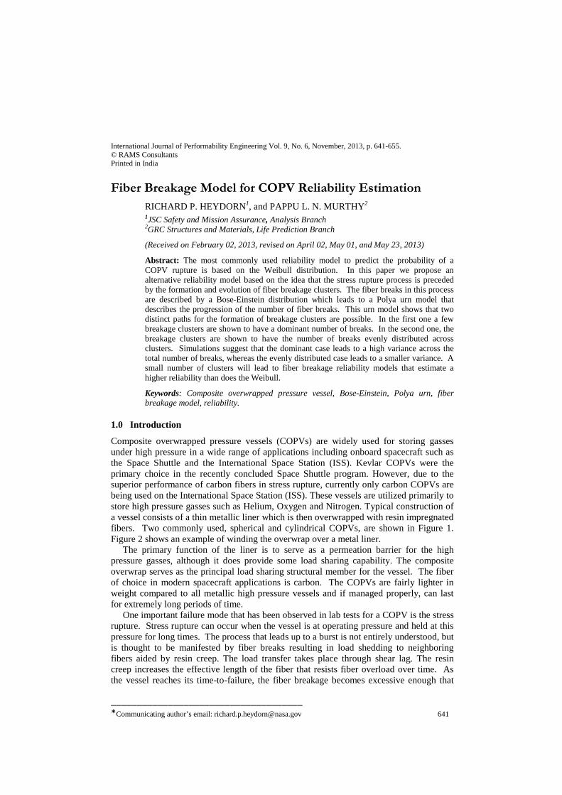
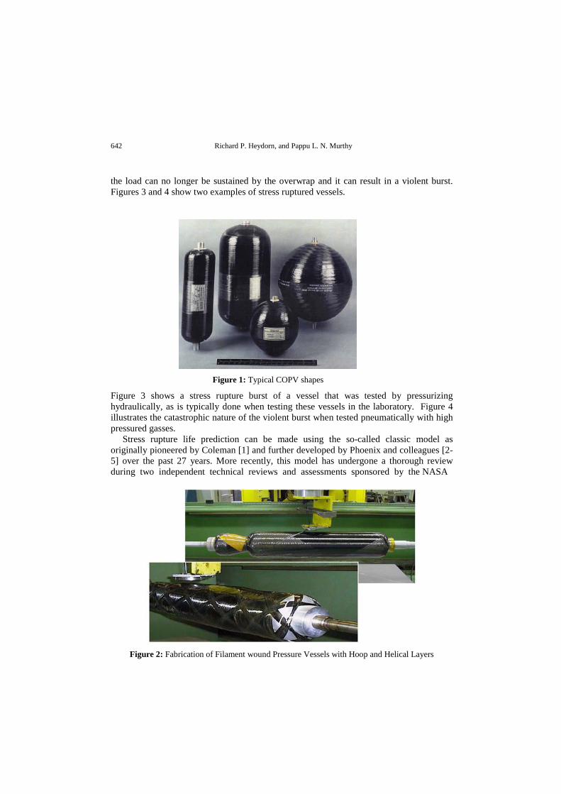
Composite overwrapped pressure vessels (COPVs) are widely used for storing gasses under high pressure in a wide range of applications including onboard spacecraft such as the Space Shuttle and the International Space Station (ISS). Kevlar COPVs were the primary choice in the recently concluded Space Shuttle program. However, due to the superior performance of carbon fibers in stress rupture, currently only carbon COPVs are being used on the International Space Station (ISS). These vessels are utilized primarily to store high pressure gasses such as Helium, Oxygen and Nitrogen. Typical construction of a vessel consists of a thin metallic liner which is then overwrapped with resin impregnated fibers. Two commonly used, spherical and cylindrical COPVs, are shown in Figure 1. Figure 2 shows an example of winding the overwrap over a metal liner. The primary function of the liner is to serve as a permeation barrier for the high pressure gasses, although it does provide some load sharing capability. The composite overwrap serves as the principal load sharing structural member for the vessel. The fiber of choice in modern spacecraft applications is carbon. The COPVs are fairly lighter in weight compared to all metallic high pressure vessels and if managed properly, can last for extremely long periods of time. One important failure mode that has been observed in lab tests for a COPV is the stress rupture. Stress rupture can occur when the vessel is at operating pressure and held at this pressure for long times. The process that leads up to a burst is not entirely understood, but is thought to be manifested by fiber breaks resulting in load shedding to neighboring fibers aided by resin creep. The load transfer takes place through shear lag. The resin creep increases the effective length of the fiber that resists fiber overload over time. As the vessel reaches its time-to-failure, the fiber breakage becomes excessive enough that

642 Richard P. Heydorn, and Pappu L. N. Murthy

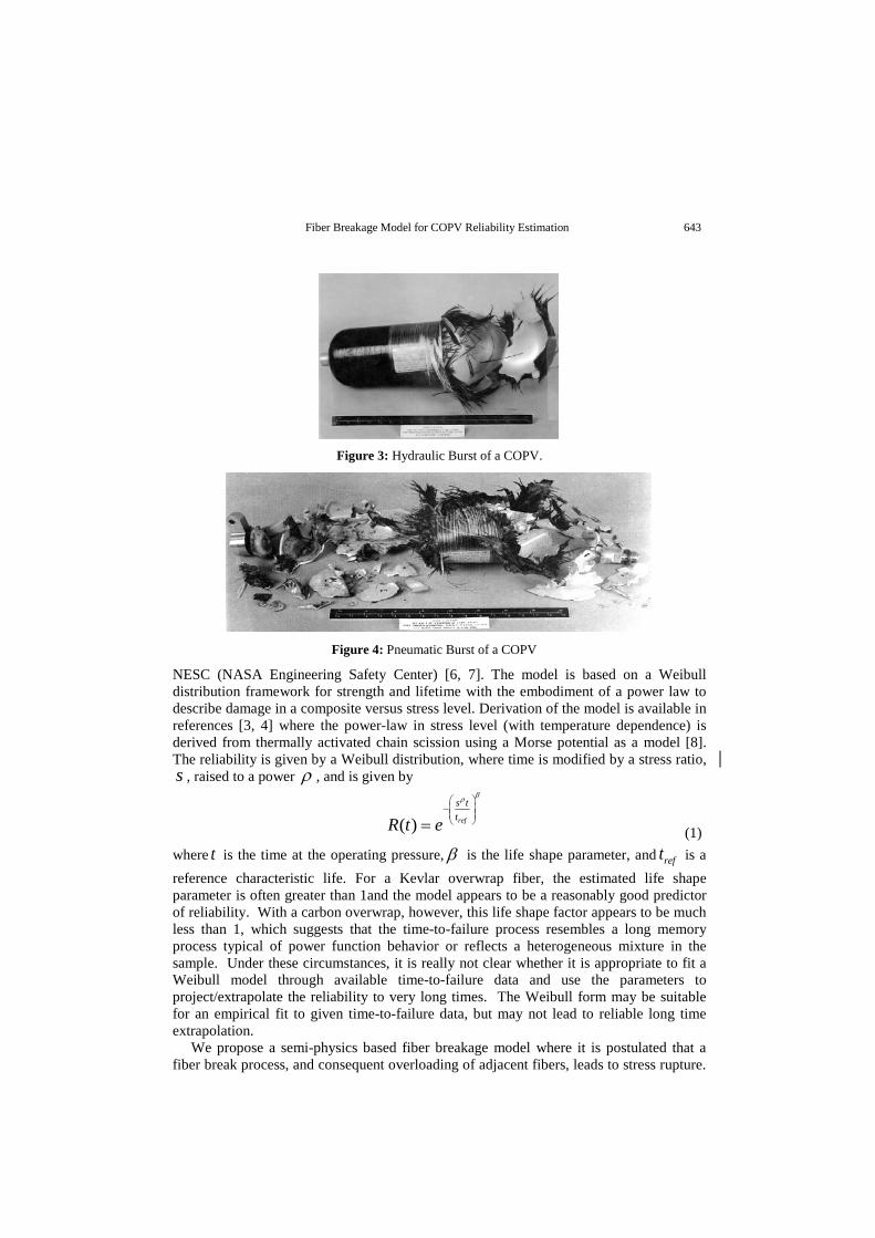
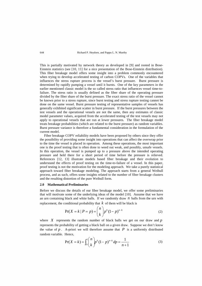
the load can no longer be sustained by the overwrap and it can result in a violent burst. Figures 3 and 4 show two examples of stress ruptured vessels.

Figure 1: Typical COPV shapes

Figure 3 shows a stress rupture burst of a vessel that was tested by pressurizing hydraulically, as is typically done when testing these vessels in the laboratory. Figure 4 illustrates the catastrophic nature of the violent burst when tested pneumatically with high pressured gasses. Stress rupture life prediction can be made using the so-called classic model as originally pioneered by Coleman [1] and further developed by Phoenix and colleagues [2-5] over the past 27 years. More recently, this model has undergone a thorough review during two independent technical reviews and assessments sponsored by the NASA

Figure 2: Fabrication of Filament wound Pressure Vessels with Hoop and Helical Layers

Fiber Breakage Model for COPV Reliability Estimation 643

Figure 3: Hydraulic Burst of a COPV.

Figure 4: Pneumatic Burst of a COPV

NESC (NASA Engineering Safety Center) [6, 7]. The model is based on a Weibull distribution framework for strength and lifetime with the embodiment of a power law to describe damage in a composite versus stress level. Derivation of the model is available in references [3, 4] where the power-law in stress level (with temperature dependence) is derived from thermally activated chain scission using a Morse potential as a model [8]. The reliability is given by a Weibull distribution, where time is modified by a stress ratio, s , raised to a power ρ , and is given by

( ) ref

s ttR t e

βρ − = (1)

where t is the time at the operating pressure, β is the life shape parameter, and reft is a reference characteristic life. For a Kevlar overwrap fiber, the estimated life shape parameter is often greater than 1and the model appears to be a reasonably good predictor of reliability. With a carbon overwrap, however, this life shape factor appears to be much less than 1, which suggests that the time-to-failure process resembles a long memory process typical of power function behavior or reflects a heterogeneous mixture in the sample. Under these circumstances, it is really not clear whether it is appropriate to fit a Weibull model through available time-to-failure data and use the parameters to project/extrapolate the reliability to very long times. The Weibull form may be suitable for an empirical fit to given time-to-failure data, but may not lead to reliable long time extrapolation. We propose a semi-physics based fiber breakage model where it is postulated that a fiber break process, and consequent overloading of adjacent fibers, leads to stress rupture.


This is partially motivated by network theory as developed in [9] and rooted in Bose-Einstein statistics (see [10, 11] for a nice presentation of the Bose-Einstein distribution). This fiber breakage model offers some insight into a problem commonly encountered when trying to develop accelerated testing of carbon COPVs. One of the variables that influences the stress rupture process is the vessel’s burst pressure. Burst pressure is determined by rapidly pumping a vessel until it bursts. One of the key parameters in the earlier mentioned classic model is the so called stress ratio that influences vessel time-to-failure. The stress ratio is usually defined as the fiber share of the operating pressure divided by the fiber share of the burst pressure. The exact stress ratio of the vessel cannot be known prior to a stress rupture, since burst testing and stress rupture testing cannot be done on the same vessel. Burst pressure testing of representative samples of vessels has generally exhibited significant scatter in burst pressure. If the burst pressures between the test vessels and the operational vessels are not the same, then any estimates of classic model parameter values, acquired from the accelerated testing of the test vessels may not apply to operational vessels that are run at lower pressures. The fiber breakage model treats breakage probabilities (which are related to the burst pressure) as random variables. Burst pressure variance is therefore a fundamental consideration in the formulation of the current model. Fiber breakage COPV reliability models have been proposed by others since they offer the possibility of providing some insight into operations that can affect the overwrap prior to the time the vessel is placed in operation. Among these operations, the most important one is the proof testing that is often done to weed out weak, and possibly, unsafe vessels. In this operation, the vessel is pumped up to a pressure above the intended operating pressure and held there for a short period of time before the pressure is relieved. References [12, 13] illustrate models based fiber breakage and their evolution to understand the effects of proof testing on the time-to-failure of a vessel. In this paper, proof testing is not the motivation for the modeling approach. We take a purely statistical approach toward fiber breakage modeling. The approach starts from a general Weibull process, and as such, offers some insights related to the number of fiber breakage clusters and the resulting distortion of the pure Weibull form.

2.0 Mathematical Preliminaries

Before we discuss the details of our fiber breakage model, we offer some preliminaries that will motivate some of the underlying ideas of the model [10]. Assume that we have an urn containing black and white balls. If we randomly draw n balls from the urn with replacement, the conditional probability that k of them will be black is

Pr( | ) (1 )k n knX k P p p p

k−

= = = −

(2)

where X represents the random number of black balls we get on our draw and p represents the probability of getting a black ball on a given draw. Suppose we don’t know the value of p . A-priori we will therefore assume that P is a uniformly distributed random variable. Hence,

1

0

1Pr( ) (1 )1

k n knX k p p dp

k n−

= = − = + ∫ (3)


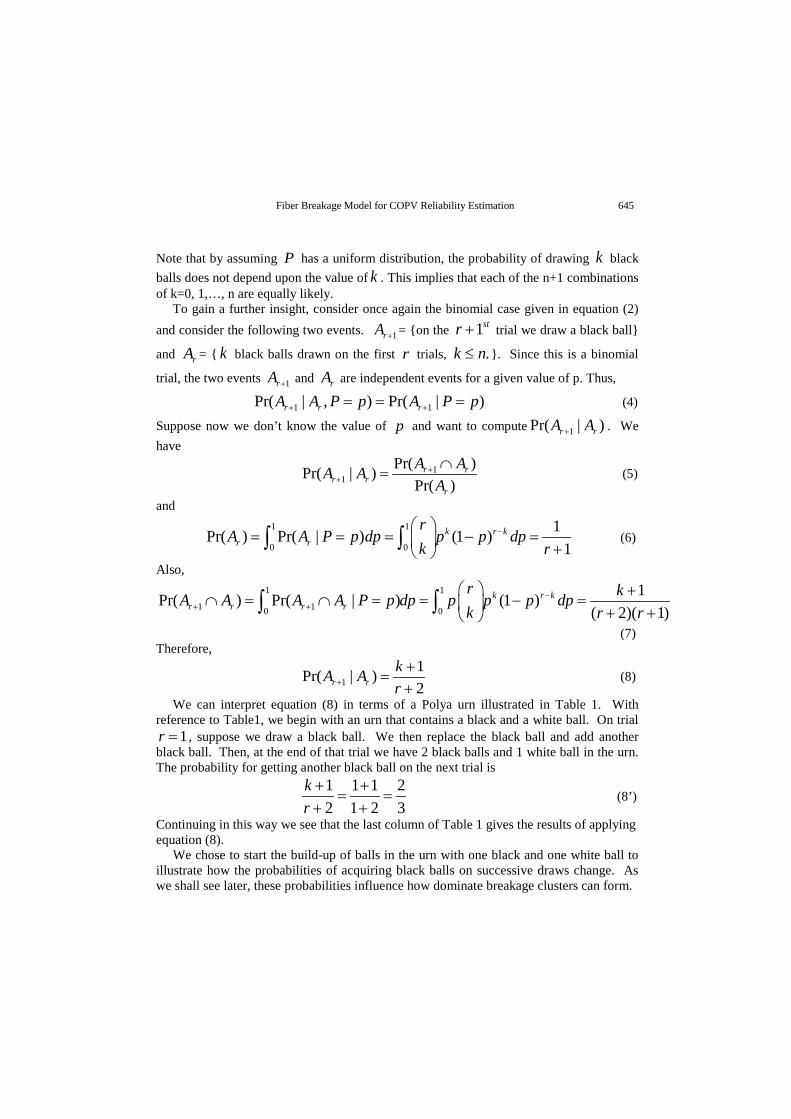
Note that by assuming P has a uniform distribution, the probability of drawing k black balls does not depend upon the value of k . This implies that each of the n+1 combinations of k=0, 1,…, n are equally likely. To gain a further insight, consider once again the binomial case given in equation (2) and consider the following two events. 1rA + = {on the 1str + trial we draw a black ball}

and rA = { k black balls drawn on the first r trials, .nk ≤ }. Since this is a binomial

trial, the two events 1rA + and rA are independent events for a given value of p. Thus,

1 1Pr( | , ) Pr( | )r r rA A P p A P p+ += = = (4)

Suppose now we don’t know the value of p and want to compute 1Pr( | )r rA A+ . We have

11

Pr( )Pr( | )Pr( )

r rr r

r

A AA AA

++

∩= (5)

and

1 1

0 0

1Pr( ) Pr( | ) (1 )1

k r kr r

rA A P p dp p p dp

k r−

= = = − = + ∫ ∫ (6)

Also,1 1

1 10 0

1Pr( ) Pr( | ) (1 )( 2)( 1)

k r kr r r r

r kA A A A P p dp p p p dpk r r

−+ +

+∩ = ∩ = = − = + +

∫ ∫ (7) Therefore,

11Pr( | )2r r

kA Ar+

+=

+ (8)

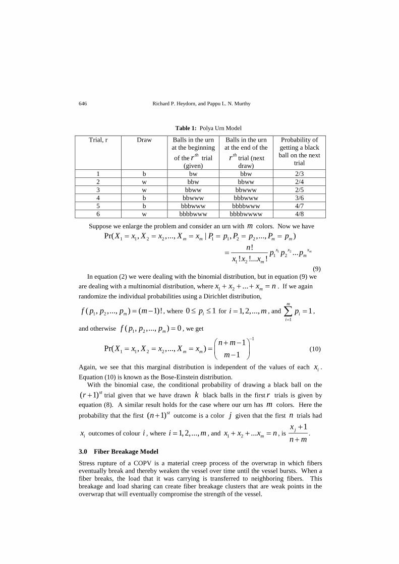
We can interpret equation (8) in terms of a Polya urn illustrated in Table 1. With reference to Table1, we begin with an urn that contains a black and a white ball. On trial

1r = , suppose we draw a black ball. We then replace the black ball and add another black ball. Then, at the end of that trial we have 2 black balls and 1 white ball in the urn. The probability for getting another black ball on the next trial is

1 1 1 22 1 2 3

kr+ +

= =+ +

(8’)

Continuing in this way we see that the last column of Table 1 gives the results of applying equation (8). We chose to start the build-up of balls in the urn with one black and one white ball to illustrate how the probabilities of acquiring black balls on successive draws change. As we shall see later, these probabilities influence how dominate breakage clusters can form.


Table 1: Polya Urn Model

Trial, r Draw Balls in the urn at the beginning of the thr trial

(given)

Balls in the urn at the end of the

thr trial (next draw)

Probability of getting a black ball on the next

trial 1 b bw bbw 2/3 2 w bbw bbww 2/4 3 w bbww bbwww 2/5 4 b bbwww bbbwww 3/6 5 b bbbwww bbbbwww 4/7 6 w bbbbwww bbbbwwww 4/8

Suppose we enlarge the problem and consider an urn with m colors. Now we have

1 1 2 2 1 1 2 2Pr( , ,..., | , ,..., )m m m mX x X x X x P p P p P p= = = = = =

1 21 2

1 2

! ...! !... !

mxx xm

m

n p p px x x

=

(9)

In equation (2) we were dealing with the binomial distribution, but in equation (9) we are dealing with a multinomial distribution, where nxxx m =+++ ...21 . If we again randomize the individual probabilities using a Dirichlet distribution,

1 2( , ,..., ) ( 1)!mf p p p m= − , where 0 1ip≤ ≤ for 1, 2,...,i m= , and 1

1m

ii

p=

=∑ ,

and otherwise 1 2( , ,..., ) 0mf p p p = , we get

1

1 1 2 2

1Pr( , ,..., )

1m m

n mX x X x X x

m

−+ − = = = = −

(10)

Again, we see that this marginal distribution is independent of the values of each ix . Equation (10) is known as the Bose-Einstein distribution. With the binomial case, the conditional probability of drawing a black ball on the ( 1)str + trial given that we have drawn k black balls in the first r trials is given by equation (8). A similar result holds for the case where our urn has m colors. Here the probability that the first ( 1)stn + outcome is a color j given that the first n trials had

ix outcomes of colour i , where 1, 2,...,i m= , and 1 2 ... mx x x n+ + = , is 1jx

n m+

+.

3.0 Fiber Breakage Model

Stress rupture of a COPV is a material creep process of the overwrap in which fibers eventually break and thereby weaken the vessel over time until the vessel bursts. When a fiber breaks, the load that it was carrying is transferred to neighboring fibers. This breakage and load sharing can create fiber breakage clusters that are weak points in the overwrap that will eventually compromise the strength of the vessel.


We will assume that this cluster formation process will be based on an a-priori given number of clusters. While this may seem somewhat artificial, we will see that the number of clusters determine the eventual reliability model that will form. To begin, let’s assume that only 2 clusters will be formed. As in Table 1, one cluster will be labeled the black cluster, and the other the white cluster. As in Table 1, suppose the first break occurs in the black cluster. This means that the fibers surrounding the broken fiber take up the load shed by the broken fiber. Consequently, the load on the black cluster increases and this is represented by adding another black ball to that cluster. Note in Table 1, this has the effect of increasing the probability of breakage of the black cluster from 1

2 (not shown in the Table) to 2

3 . The probability of breakage occurring in the white cluster is decreased from 1

2 to 13 . While we have named the clusters black and white, we will assume that

the breakage process remains unchanged if we switch the names of the clusters. The effect on the propensity to cause the vessel to burst is assumed to remain the same. This assumption is in line with the use of the Bose-Einstein distribution. That is, clusters are inherently unrecognizable. As we proceed down the last column of Table 1, we see how the probability of cluster breakage is evolving. In reality, however, it is not clear how much load is transferred when a fiber breaks. As we shall see later, this load sharing process is meant to determine the family of the breakage model. Given data related to the time-to-failure and stress ratios, we can estimate parameter values that will determine the member of the family that is operational. We have also not addressed at this point how the fiber strength varies across the overwrap. This variation in strength is likely to be related to the number of breakage clusters that can form and thereby determines the model family that will best match the data.

4.0 Reliability Estimation: The Binomial Case

Next, we consider a model for the growth of the total number of breaks that occur over time starting at time 0. Let that number be ( )N t . For 0,1, 2,...n = let

( )Pr( ( ) )

!

nttN t n e

nβ

βλλ −= = (11)

where 1λη

= and η is the characteristic life of this Weibull process. Consider the case

where ( )N t breaks occur and k of them occur in a given cluster, where there are two breakage clusters, such that the vessel does not fail. It will be shown that the final results are not dependent on these particular assumptions. The reliability for this case is then defined as

( )( )( ) (1 )k N t kN t

R t E P Pk

− = −

(12)

Here P is a random probability of having a fiber break in the black cluster. Using equations (2) and (12), we have that


( )( )( ) (1 ) | ( )k N t kN t

R t E E P P N tk

−

= −

(13)

and therefore,

β

λλ

β

λλ

ββ

tee

nt

ndppp

ktN

EtRt

n

tn

ktNk−∞

=

−− −=

+=

−

= ∑∫

1!)(

11)1(

)()(

0

1

0

)(

(14) Note that the expression in equation (12) has the properties of a reliability function. It is clear that as ∞→t , )(tR approaches 0. As 0→t , by L’Hospital’s rule, 1)( →tR . Finally, it is clearly a decreasing function. Note also that it would appear that this reliability expression is a function of k , where )(0 tNk ≤≤ , but as seen in equation (3), the integral is not a function of k , and neither is the random process,

,...}2,1,0),({ =ttN , and so we can sum from 0=n to ∞=n in the summation. Finally, to determine that the final expression, on the right side of equation (14), is a good estimate of the desired reliability, we will require that the parameters λ and β are

chosen to minimize the mean square error for each sampled time-to-failure, Mttt ,...,, 21 .

That is, ∑=

−

−−

M

i i

t

ie tetR

M

i

1

21)(1

β

λ

λ

β

is to be a minimum, where )( ie tR is the

empirical reliability function evaluated at it .

5.0 Reliability Estimation: The Multinomial Case

Suppose now that we specify that a-priori we have m clusters, where 2>m . In this case we have the Dirichlet distribution to describe the cluster breakage probabilities. In place of equation (12), we have

1 21 2

1 2

( )( ) ...

, ,..,mxx x

mm

N tR t E P P P

x x x

=

(15)

Thus, using equation (10),

1 21 2

01 2

( ) !( 1)! ( )( ) ... | ( ), ,.. , ( 1)! !

m

nxx x t

mnm

N t n m tR t E E P P P N t ex x x n m n

ββ

λλ∞−

=

−= = + −

∑ (16) Indeed, the inner expectation in equation (16) is the Bose-Einstein distribution, for a fixed value of ( )N t , that is given in equation (10). The outer expectation is the average of the Bose-Einstein distribution treating { ( )}N t as a Weibull process as given in equation (11). Now,

1

10 0

!( 1)! ( ) ( 1)! ( )( 1)! ! ( ) ( 1)

n n mt t

mn n

n m t m te en m n t n m

β ββ β

λ λβ

λ λλ

+ −∞ ∞− −

−= =

− −=

+ − + −∑ ∑ (17)


Since,

0

( )1!

nt

n

t en

ββ

λλ∞−

=

=∑ (18)

it follows that,

( 1) 2

0 0

( ) ( )1( 1)! !

n m nmt t

n n

t te en m n

β ββ β

λ λλ λ+ −∞ −− −

= =

= −+ −∑ ∑ (19)

Therefore,

−

−= ∑

−

=

−−

2

01 !

)(1)(

)!1()(m

n

tn

m ent

tmtR

βλβ

β

λλ

(20)

We see that if 2=m , equation (20) reduces to equation (14). On the other hand, if we let ∞→m , we have the following proposition, Proposition 1:

−

−= ∑

−

=

−−∞→

−2

01 !

)(1)(

)!1(limm

n

tn

mmt e

nt

tme

ββ λβ

βλ λ

λ (21)

Proof: 2

0 1

( ) ( )1! !

n nmt t

n n m

t te en n

β ββ β

λ λλ λ− ∞− −

= = −

− = =∑ ∑

1 1( ) ( ) ( ) ...

( 1)! ( )! ( 1)!

m m mt t tt t te e e

m m mβ β β

β β βλ λ λλ λ λ− +

− − −+ + +− +

(22)

Therefore, 2

10

( 1)! ( )1( ) !

nmt

mn

m t et n

ββ

λβ

λλ

−−

−=

−−

∑

2 31 ( ) ( ) ...

( 1) ( 2)( 1)t t t tt te t e e e

m m m mβ β β β

β βλ β λ λ λλ λλ− − − −

= + + + + + + +

(23)

For 2>m , increasing the sum in the parentheses in right side of equation (23) by teβλ−

while also letting 1m = in that sum, we have the following inequality


2 3

2 3

( ) ( ) ...( 1) ( 2)( 1)

1 ( ) ( ) 1...2! 3!

t t t

t t t t

t t te e em m m m m m

t te t e e em m

β β β

β β β β

β β βλ λ λ

β βλ β λ λ λ

λ λ λ

λ λλ

− − −

− − − −

+ + ++ + +

< + + + + =

(24)

where we used the fact that: 2 3( ) ( ) ... 1

2! 3!t t t tt te t e e eβ β β β

β βλ β λ λ λλ λλ− − − −

+ + + + =

(25)

Hence, Proposition 1 follows. From proposition 1, if we allow for an infinite number of clusters, then the fiber breakage model reduces to a Weibull model. The next proposition shows that, for a given characteristic life, 1λ− , and a given life shape factor value, β , the resulting Weibull reliability will be less than a corresponding (same λ and β values) fiber breakage reliability. Proposition 2:

2

10

( 1)! ( )1( ) !

nmt t

mn

m te et n

β ββ

λ λβ

λλ

−− −

−=

−≤ −

∑

(26)

Proof: For 2m = in equation (14), the hazard rate, ( )h t , is

11

( ) ln( ( ))1 1

tt

t

t t

e ed t e th t R t tdt t te e

ββ

β

β β

λλ

β λ ββ

λ λ

λβ β β λλ

−−

− −

− −

−−

= − = − = − −

(27)

But since the hazard rate is nonnegative, it follows that 1 t

t eet

ββ

λλ

βλ

−− −

≤ . Therefore, the

proposition holds for 2m = . Assume it holds for an arbitrary 2om > . Consider

1om + , and consider, using equation (20), the following expression,

1 2

1 10

( 1 1)! ( )1( ) !

o

o

m nto

mnt

m t et n

e

β

β

βλ

β

λ

λλ

+ −−

+ −=

−

+ − −

∑ (28)

Now,


( )

( )

1

10

( )( )1 ! ( ) ( )! ...! 1 !

o

ooo

nm ntt

mmn mn

t to o

tt ee n t tnm me e

ββ

β β

ββλλ

β β

λ λ

λλλ λ

∞−−−

+==

− −

−= = + +

+

∑∑ (29)

Using expression (28), we have from equation (29) ( )

( ) ( )1! ( ) ( ) ... 1 ... 1

( ) ! 1 ! 1

oo

o

mmo

mo o o

m t t tt m m m

β β β

β

λ λ λλ

+ + + = + + ≥ + +

(30)

Therefore, by induction Proposition 2 holds. The multinomial case relates to an extended Polya urn where instead of having just balls of two colors, we have balls of m colors. Thus, when a breakage cluster is formed, the resulting load sharing process leads to a weakening of the breakage point that is represented as adding an extra ball of the same color as the cluster where the breakage occurred. In effect, this leads to a reduction of the average strength of the vessel overwrap over time.

6.0 The Convergence of Cluster Formation

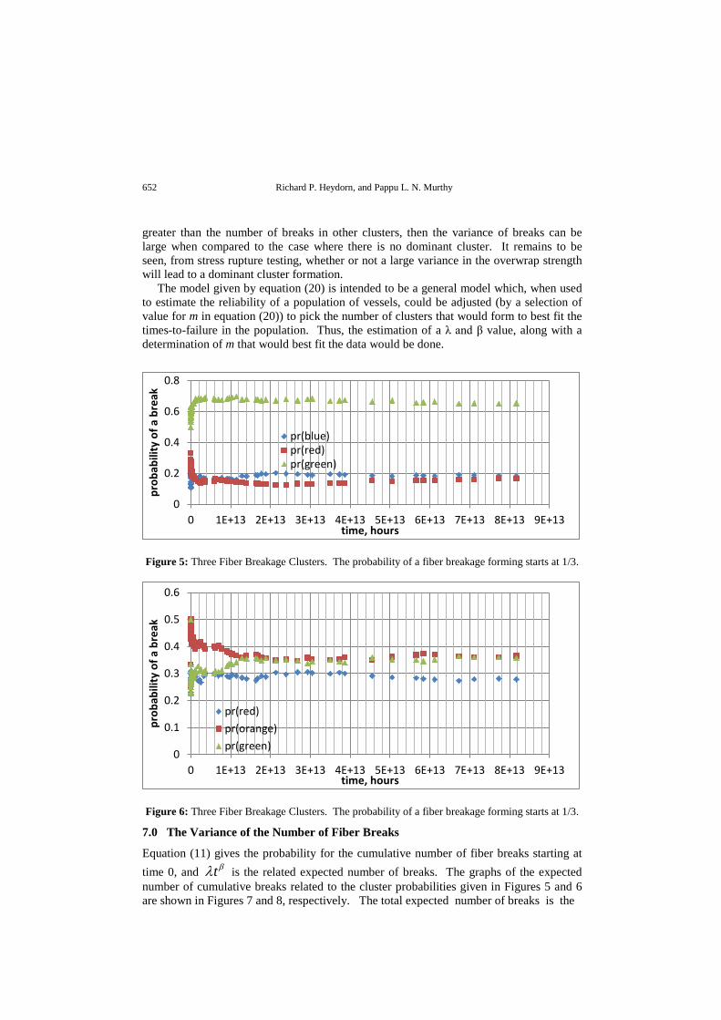
As pointed out above, the Polya urn model for the probability of a cluster formation is a consequence of the fact that we have assumed that, with regard to stress rupture, the location of each cluster is not important. Rather, it is the aggregate of clusters and their probability of breakage that determines the stress rupture process. We have assumed that we know the number of clusters that will form and it is this number that affects the divergence of the reliability distribution from a pure Weibull form. As the number of assumed clusters increase, the reliability models tend to approach a Weibull. Within this model framework we cannot know how many clusters will form prior to any stress rupture test, since this approach is not rooted in a materials study of the overwrap. This means that any determination of the most probable model will depend upon how each model fits the stress rupture test data. The number of breakage events in the model is determined by a Weibull process. For a given random path in this process, we can study the number of breakage events over time. Using the Polya urn model to represent breakage events, the probabilities of breakage events tend to oscillate as the number of total breakage events increase. Thus, it is instructive to determine when these breakage probabilities stabilize, since this can indicate if fiber breakage is concentrating on just a few clusters or if fiber breakage tends to be uniformly distributed over the overwrap. A few example cases of breakage probabilities are simulated and their graphs are shown in Figures 5 and 6 (see [14] for a Polya urn algorithm). The graph in Figure 5 illustrates the case where one cluster tends to dominate the other two shortly after cluster breakage starts. In Figure 6 the probabilities of cluster breakage do not diverge as much at the start and as the times of breakage events increase, they tend to converge. The difference between these two figures demonstrates the “luck of the draw” from the Polya urn. That is, by pure chance a single cluster will dominate, while in other cases there tends to be a more even formation of clusters. However, in terms of the stress rupture of a vessel, this luck of the draw is most likely to be influenced by the strength variance of the overwrap across the vessel surface. Areas where the strength is below the average may be ideal areas for the initiation and growth of a cluster. As we will see, in the next section, that if the number of breaks in one cluster is much


greater than the number of breaks in other clusters, then the variance of breaks can be large when compared to the case where there is no dominant cluster. It remains to be seen, from stress rupture testing, whether or not a large variance in the overwrap strength will lead to a dominant cluster formation. The model given by equation (20) is intended to be a general model which, when used to estimate the reliability of a population of vessels, could be adjusted (by a selection of value for m in equation (20)) to pick the number of clusters that would form to best fit the times-to-failure in the population. Thus, the estimation of a λ and β value, along with a determination of m that would best fit the data would be done.

Figure 5: Three Fiber Breakage Clusters. The probability of a fiber breakage forming starts at 1/3.

Figure 6: Three Fiber Breakage Clusters. The probability of a fiber breakage forming starts at 1/3.

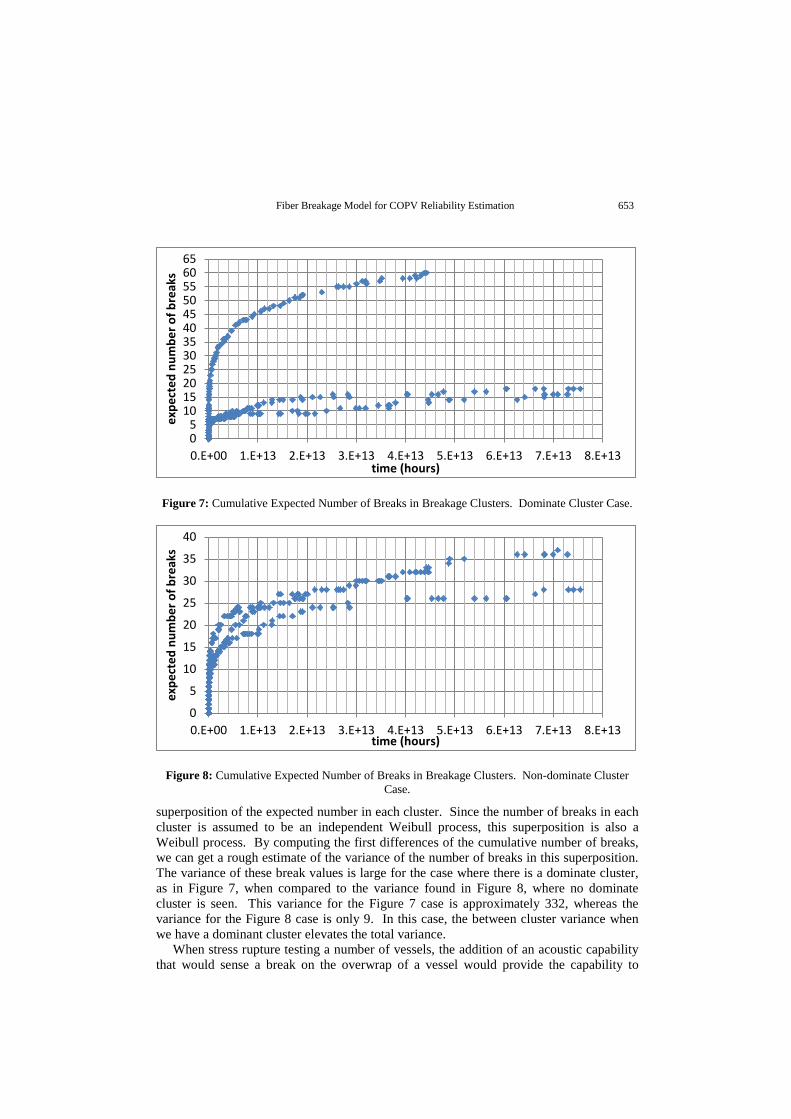
7.0 The Variance of the Number of Fiber Breaks

Equation (11) gives the probability for the cumulative number of fiber breaks starting at time 0, and t βλ is the related expected number of breaks. The graphs of the expected number of cumulative breaks related to the cluster probabilities given in Figures 5 and 6 are shown in Figures 7 and 8, respectively. The total expected number of breaks is the

0

0.2

0.4

0.6

0.8

0 1E+13 2E+13 3E+13 4E+13 5E+13 6E+13 7E+13 8E+13 9E+13

prob

abili

ty o

f a b

reak

time, hours

pr(blue)pr(red)pr(green)

0

0.1

0.2

0.3

0.4

0.5

0.6

0 1E+13 2E+13 3E+13 4E+13 5E+13 6E+13 7E+13 8E+13 9E+13

prob

abili

ty o

f a b

reak

time, hours

pr(red)pr(orange)pr(green)


Figure 7: Cumulative Expected Number of Breaks in Breakage Clusters. Dominate Cluster Case.

Figure 8: Cumulative Expected Number of Breaks in Breakage Clusters. Non-dominate Cluster Case.

superposition of the expected number in each cluster. Since the number of breaks in each cluster is assumed to be an independent Weibull process, this superposition is also a Weibull process. By computing the first differences of the cumulative number of breaks, we can get a rough estimate of the variance of the number of breaks in this superposition. The variance of these break values is large for the case where there is a dominate cluster, as in Figure 7, when compared to the variance found in Figure 8, where no dominate cluster is seen. This variance for the Figure 7 case is approximately 332, whereas the variance for the Figure 8 case is only 9. In this case, the between cluster variance when we have a dominant cluster elevates the total variance. When stress rupture testing a number of vessels, the addition of an acoustic capability that would sense a break on the overwrap of a vessel would provide the capability to

05

101520253035404550556065

0.E+00 1.E+13 2.E+13 3.E+13 4.E+13 5.E+13 6.E+13 7.E+13 8.E+13

expe

cted

num

ber o

f bre

aks

time (hours)

0

5

10

15

20

25

30

35

40

0.E+00 1.E+13 2.E+13 3.E+13 4.E+13 5.E+13 6.E+13 7.E+13 8.E+13

expe

cted

num

ber o

f bre

aks

time (hours)


estimate the breakage variance and thereby sense the formation of a dominate, or possibly, the formation of a few dominate clusters.

8.0 Implications of an Increasing Number of Breakage Clusters

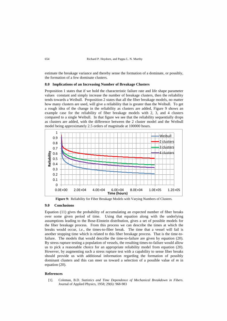
Proposition 1 states that if we hold the characteristic failure rate and life shape parameter values constant and simply increase the number of breakage clusters, then the reliability tends towards a Weibull. Proposition 2 states that all the fiber breakage models, no matter how many clusters are used, will give a reliability that is greater than the Weibull. To get a rough idea of the change in the reliability as clusters are added, Figure 9 shows an example case for the reliability of fiber breakage models with 2, 3, and 4 clusters compared to a single Weibull. In that figure we see that the reliability sequentially drops as clusters are added, with the difference between the 2 cluster model and the Weibull model being approximately 2.5 orders of magnitude at 100000 hours.

Figure 9: Reliability for Fiber Breakage Models with Varying Numbers of Clusters.

9.0 Conclusions

Equation (11) gives the probability of accumulating an expected number of fiber breaks over some given period of time. Using that equation along with the underlying assumptions leading to the Bose-Einstein distribution, gives a set of possible models for the fiber breakage process. From this process we can describe the times at which the breaks would occur, i.e., the times-to-fiber break. The time that a vessel will fail is another stopping time which is related to this fiber breakage process. That is the time-to-failure. The models that would describe the time-to-failure are given by equation (20). By stress rupture testing a population of vessels, the resulting times-to-failure would allow us to pick a reasonable choice for an appropriate reliability model from equation (20). However, by augmenting such a stress rupture test with a capability to sense fiber breaks should provide us with additional information regarding the formation of possibly dominant clusters and this can steer us toward a selection of a possible value of m in equation (20).

References [1]. Coleman, B.D. Statistics and Time Dependence of Mechanical Breakdown in Fibers.

Journal of Applied Physics, 1958; 29(6): 968-983

00.10.20.30.40.50.60.70.80.9

1

0.0E+00 2.0E+04 4.0E+04 6.0E+04 8.0E+04 1.0E+05 1.2E+05

Relia

bilit

y

Time (hours)

Weibull2 clusters3 clusters4 clusters


[2]. Phoenix, S.L., and E.M. Wu. Statistics for the Time Dependent Failure of Kevlar-49/Epoxy Composites: Micromechanical Modeling and Data Interpretation. IUTAM Symposium on Mechanics of Composite Materials. Pergamon 1983:135-164.

[3]. Phoenix, S.L. Statistical Modeling of the Time and Temperature Dependent Failure of Fibrous Composites. Proceedings of the 9th US National Congress of Applied Mechanics, Book # H00228, ASME, NY 1982: 219-229.

[4]. Phoenix, S.L. The Asymptotic Time to Failure of a Mechanical System of Parallel Members. SIAM Journal on Applied Mathematics, 1978; 34 (2): 227-246.

[5]. Phoenix, S.L. Stochastic Strength and Fatigue of Fiber Bundles. International Journal of Fracture, 1978; 14(3): 327-344.

[6]. Cameron, K.D., L. Grimes-Ledesma, P.L.N. Murthy, J. K. Sutter, S. L. Phoenix, and R. Saulsberry. Orbiter Kevlar/Epoxy Composite Overwrapped Pressure Vessel Flight Rationale Technical Assessment Report, Vol. I and II, NASA NESC Report RP-07-34, April 12, 2007.

[7]. Cameron, K.D., et.al. Shelf Life Phenomenon and Stress Rupture Life of Carbon/Epoxy Composite Overwrapped Pressure Vessels (COPVs) Technical Consultation Report. Vol. I and II, NASA NESC Report RP-06-83, September 14, 2006.

[8]. Glaser, R.E., R. L. Moore, and T. T. Chiao. Life Estimation of Aramid/Epoxy Composites under Sustained Tension. Composites Technology Review, 1984; Vol. 6: 26-35.

[9]. Bianconi, Ginestra, Barabasi, Albert-Laszlo. Bose-Einstein Condensation in Complex Networks. Physical Review Letters, 2001; 86(24): 5633-5635.

[10]. Sheldon, R. M., Introduction to Probability Models. Academic Press, 2007. [11]. Johnson, N. L., S. L. Kotz. Urn Models and Their Application, An Approach to Modern

Discrete Probability Theory. John Wiley and Sons, 1977. [12]. Murthy, P. L.N., S. L. Phoenix, and L. Grimes-Ledesma. Fiber Breakage Model for

Carbon Composite Stress Rupture Phenomenon: Theoretical Development and Applications. NASA/TM – 2010-215831, March 2010.

[13]. Reeder, J. R. A Critique of a Phenomenological Fiber Breakage Model for Stress Rupture of composite Materials, NASA/TM – 2010-216721, July 2010.

[14]. Hand, C. History Matters: Modeling Path Dependence on a Spreadsheet. CHEER, 2006; 18 (1): 19-24.

Richard P. Heydorn received a B.E.E. in Electrical Engineering and a M.A. in Mathematics from the University of Akron. He has a Ph.D. in Statistics from the Ohio State University. He was an adjunct professor at the University of Houston at Clear Lake where he taught statistics and is currently an adjunct professor at Rice University. At the Johnson Space Center he is in the S&MA analysis branch working on COPV and software reliability models. Pappu L. N. Murthy got his Doctorate from School of Aerospace engineering in 1982 at Georgia Institute of Technology, Atlanta, GA. Since 1982, he joined as post-doctoral research fellow at NASA Glenn Research Center and subsequently joined the civil service at NASA Glenn. He has been working exclusively in Composite Mechanics, Probabilistic Methods and Analysis areas and has published over 300 papers including the NASA TMs, Conference Proceedings and journal articles.

Documents

Fiber Breakage Model for COPV Reliability Estimationparis.utdallas.edu/IJPE/Vol09/Issue06/pp.641-655 IJPE 480 13... · Simulations suggest thatthe dominant case leads to a high variance