International Journal of Performability Engineering, Vol. 11, No. 5, September 2015, pp. 427-442. © RAMS Consultants Printed in India

____________________________________________________ *Communicating author’s email: monika.tanwar79@gmail.com 427

Maintenance Modelling using Generalized Renewal Process for Sequential Imperfect Corrective and Preventive Maintenance

MONIKA TANWAR*and NOMESH BOLIA Department of Mechanical Engineering, Indian Institute of Technology, Hauz Khas, New Delhi, INDIA.

(Received on March 11, 2015, revised on July 4, 2015)

Abstract: The paper attempts to model the imperfect repair with the concept of arithmetic reduction of age (ARA) and also sequentially incorporates the effect of imperfect corrective and preventive maintenance. Four virtual age processes are devised to describe the various after repair restoration patterns as well as different restoration degrees for both CM and PM. The GRP maximum likelihood estimators (MLE) are derived and then used for parameter estimation. The expected number of failures for the proposed approaches are estimated using Monte Carlo simulation. Two different repair effectiveness indices for CM and PM are estimated for all the four approaches to provide a better insight of the maintenance processes. The residual life is predicted using residual mean time to failure based on virtual age at each repair point. The paper concludes with comparative analysis to get adequate insights into the goodness of fit for the proposed models.

Keywords: Repairable systems, imperfect CM, imperfect PM, repair effectiveness, restoration patterns

1. Introduction

Maintenance management of various manufacturing processes, power, and service industries (e.g., aviation, railways etc.) deals with large scale maintenance of equipment to reduce disruptions in production and services. Maintenance actions are required either to prevent a failure or to restore equipment to a specified state. Thus maintenance can be categorized into (a) corrective maintenance (CM) which is carried out after failure, (b) preventive maintenance (PM) that is carried out periodically to prevent failures. In general perfect maintenance which restores the system to an ‘as good as new condition’ (AGAN) is modeled using a renewal process (RP), and minimal repair which brings back the system to ‘as bad as old condition’ (ABAO), is modelled through Non Homogenous Poisson Process (NHPP). Imperfect maintenance models attempt to incorporate repairable systems that can also arrive at ‘better than old but worse than new’, ‘better than new’, or ‘worse than old’ states. Mathematical models for these after-repair states are much more complex but appropriate for modeling real operating conditions. A literature review on imperfect repairs is presented in the rest of this section. Nakagawa [1], [2] models imperfect repair by developing (p, q) rule and applies it to obtain optimum PM policies. Brown and Proschan [3] then consider that the repair actions are either perfect with probability p or minimal with probability (1- p) and develop optimal replacement policies. Block et al. [4] extends the Brown Proschan model by including the age ‘t’ of the component and their result came to be known as (p (t), q (t)) rule. Kijima and Sumita [5], [6] introduce the idea of the “virtual age” for imperfect repairs and generalize the g-renewal equation for imperfect repairs. Kijima I (KI) and Kijima II (KII) are the two widely used types of virtual age models considering different after repair restoration possibilities, i.e., restoration of latest operating age (latest time

428 Monika Tanwar and Nomesh Bolia

between failure) and restoration of complete operating age (since new) respectively. Most of the virtual age models are tailored for “wearing-out systems”, that are described by reliability models with increasing failure intensity but in practice the shape of the intensities can be decreasing or even more complex, for instance bathtub shaped intensity. It is therefore desirable to generalize imperfect maintenance models for all classes of initial intensities. Dijoux [7] proposes a virtual age model when the initial intensity is bathtub shaped. This intensity considers all the three phases of the life cycle of equipment that includes a burn-in-period, where risk of failure is weak, useful life period where the failures are random in nature and finally a wear-out period. Another approach of failure intensity reduction known as ARI (arithmetic reduction of intensity) models is discussed in detail by Doyen and Gaudoin [8]. A new reliability model [7] based on the earlier models [9] is developed that combines bathtub shaped life and imperfect maintenance through virtual age models. The models available for imperfect repairs mainly consider CM to be imperfect and PM to be either perfect or ‘ABAO’. Hence the PMs are modeled through either RP or NHPP. However, few attempts to model both CMs and PMs as imperfect repairs are made in the literature as discussed below. Kijima et al. [5], [9] first used the notion of decrease in virtual age to model the performance of a system with imperfect CM, and periodic replacement. Jack [10] ; Doyen and Gaudoin [11]; Ramirez and Utne [12] utilize the concept of virtual age to model the effect of both imperfect CM and imperfect periodic PM. Authors [12] further provide decision support model for continuously operated system and safety systems that operate on demand and are under CM as well as PM. This is a step forward in research as the authors consider repair effectiveness for both PM and CM. Hurtado et al. [13] use genetic algorithm to solve MLE equation for parameter estimation. Liu et al. [14] utilize virtual age concept for modeling of imperfect periodic PM and minimal CM. Further, detailed reviews [15], [16] discuss imperfect maintenance models in general and virtual age models in specific. The seldom discussed Kijima II virtual model is deliberated and MLEs for single and multiple repairable systems are discussed by Mettas and Zhao [17] for imperfect CM. Imperfect repair models for repairable system generally consider three parameters i.e., shape parameter, scale parameter and repair effectiveness (either for PM or CM). A single repair effectiveness index for both CM and PM may not provide a realistic model since both have different impacts on the system. In this paper four virtual age models are formulated to provide imperfect maintenance parameters based on failures as well as scheduled maintenance activities. The simultaneous estimation of repair effectiveness index for CM and PM makes the proposed imperfect repair models robust and more suitable than the existing methodology of using a single repair effectiveness measure. Further optimization of such models leads to more effective maintenance policies. An overhaul cycle (rebuilding or as good as new state) is therefore considered with the sequential imperfect CM and PM to build up the proposed methodologies and the models. The proposed models relax the above discussed limitations as well as consider all possible after-repair restoration patterns, i.e., restorations of latest operating time between failures, restoration of ages since new and combined restoration of latest operating time between failures, as well as restoration of age since new using both CM and PM. The contribution of the paper mainly lies in modeling the virtual age models with sequential repair effectiveness indices for both CM and PM considering four different situations rarely considered in the literature. Furthermore the paper brings out the methodology for computing MLEs of all the performance parameters by two different

Maintenance Modelling using Generalized Renewal Process for Sequential 429 Imperfect Corrective and Preventive Maintenance

methods. The first method of obtaining MLEs is by modeling the likelihood function as a constraint optimization problem. The second method finds the derivatives for directly obtaining the MLEs. The second method is not attempted in the literature for Kijima II as well as for proposed models incorporating sequential CMs and PMs. Lastly, residual life is estimated for imperfect repairs using virtual age. The models are subsequently illustrated and tested on a repairable system data.

Notation and Acronyms: ABAO As Bad As Old AGAN As Good As New BOWN Better than Old Worse than New BTN Better Than New BTO Better Than Old cdf Cumulative Distribution Function E[N(t)] Expected Number of failure F(t) Cumulative Distribution Function f(t) pdf of failure time GRP Generalized Renewal Process L(.) Likelihood function NHPP Non-Homogenous Poisson Process pdf Probability Distribution Function q Repair effectiveness for K-I and K-II

models qCM Repair effectiveness of CM qPM Repair effectiveness of PM R(t) Reliability function, 1-F(t)

RMTTF

Residual Mean Time to Failure

RP Renewal Process vij Virtual age after ith failure in jth PM

interval xij Time between ith and (i-1)th failure in

jth PM interval α Characteristic life β Shape parameter λ(t) Failure intensity at time t MTBF Mean Time Between Failure FM Failure Mode CM Corrective Maintenance PM Preventive Maintenance K I Kijima Virtual age model-I K II Kijima Virtual age model-II f(xi/vi-1) Conditional pdf of xi given vi-1 vj Virtual age after jth PM nj Number of failures in jth PM Interval

2. GRP Modeling for Imperfect CM and Imperfect PM

To address the existing uncertainties resulting from the assumptions of AGAN and ABAO, GRP modelling for both sequential imperfect PM and CM is presented in this section. Kijima and Sumita [5] develop an imperfect repair model using GRP for the virtual age (vn) of a repairable system. Here vn represents the calculated age of the system instantly after the nth repair occurs. If vn= y, then the system has a time to the (n + 1)th failure, x n+1, which is distributed according to the following cdf:

F(X|Vn = y) = F(x+y)−F(y)1−F(y)

(1) where F(x) is the cdf of the Time to first failure (TTFF) distribution of a new system or component. Kijima develop two models for imperfect repair as discussed in the earlier sections. Both are presented in subsequent sections.

2.1 Kijima-I

The virtual age computation is described in detail by Kijima (1989). The repair is assumed to have restoration only for the accumulated damage during time between ith and (i-1)th failure and is termed the Kijima-I model:

vn = q∑ Xini=1 (2)

where vn is the virtual age after nth failure; xi is the time between ith and (i-1)th failure and q is the repair effectiveness index. For further analysis Weibull distribution is assumed for time to first failure and conditional probability of survival is used for subsequent failures. The model is further modified and MLEs for the parameter estimation are developed and

430 Monika Tanwar and Nomesh Bolia

numerical solution for MLEs, expected number of failures are provided in detail by Yanez et al. [18].

2.2 Kijima-II

Another virtual age model proposed by Kijima is termed Kijima-II where the repair action at any point of time restores the entire accumulated age since new and is given by:

vn = qxn + q∑ qn−1n−1i=1 xi (3)

where vn is the virtual age after nth failure; xn is the time between failure in nth and (n-1)th failure; xi is the time between ith and (i-1)th failure and q is the repair effectiveness index. The MLEs are derived for the failure and time terminated data followed by a discussion on the applicability of Kijima-II model. The pdf for Kijima-II is given by:

f(xi + vi−1|vi−1) = βαβ

(xi + vi−1)β−1 × exp ��vi−1α�β− �xi+vi−1

α�β� (4)

The failure and time terminated MLEs are further derived by differentiating the respective likelihood functions with respect to α, β, q and equating them to zero. The failure terminated MLEs can be derived by taking partial derivative of likelihood function [19] with respect to α, β, and q and the equations are given in Appendix A. Similarly, time terminated MLEs for Kijima- II can be derived and is shown in Appendix B. The expected number of failures can be estimated using the cdf for Kijima-II:

F(ti) = 1 − exp ��qα∑ qn−jxji−1j−1 �

β− �

qxi+q∑ qn−jxji−1j=1

α�β

� (5)

Section 2.3 develops sequential imperfect virtual age models for imperfect CM and imperfect PM corresponding to the four different types of restoration patterns as described in Figures 2, 4, 5 and 6.

2.3 Model-I: Restoration of the Latest Operating Age both, by CM and PM

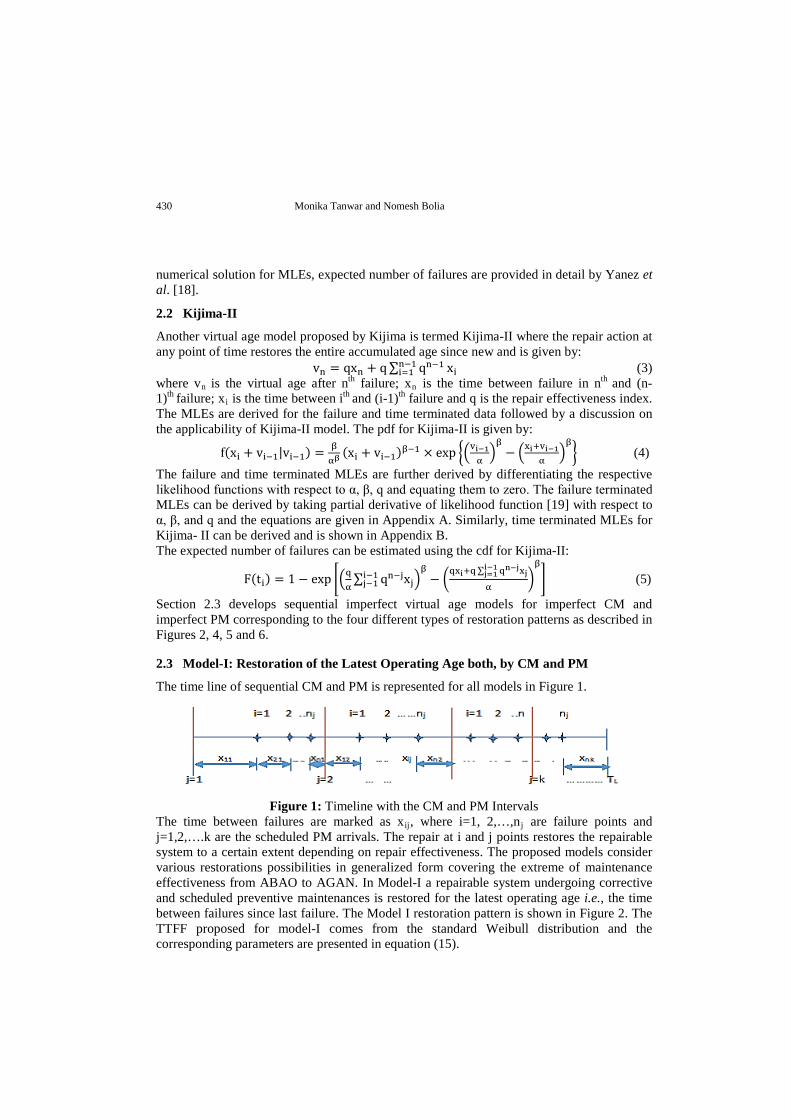
The time line of sequential CM and PM is represented for all models in Figure 1.

Figure 1: Timeline with the CM and PM Intervals

The time between failures are marked as xij, where i=1, 2,…,nj are failure points and j=1,2,….k are the scheduled PM arrivals. The repair at i and j points restores the repairable system to a certain extent depending on repair effectiveness. The proposed models consider various restorations possibilities in generalized form covering the extreme of maintenance effectiveness from ABAO to AGAN. In Model-I a repairable system undergoing corrective and scheduled preventive maintenances is restored for the latest operating age i.e., the time between failures since last failure. The Model I restoration pattern is shown in Figure 2. The TTFF proposed for model-I comes from the standard Weibull distribution and the corresponding parameters are presented in equation (15).

Maintenance Modelling using Generalized Renewal Process for Sequential 431 Imperfect Corrective and Preventive Maintenance

vi 1 j xij

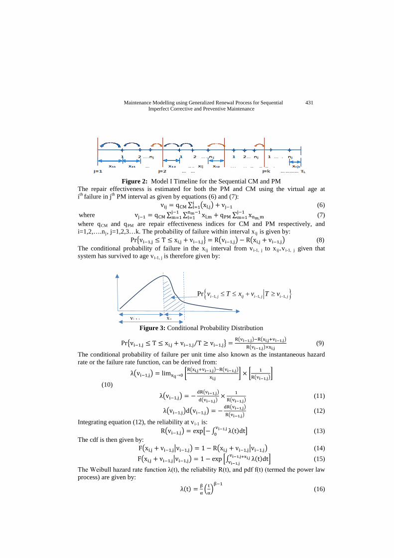
Figure 2: Model I Timeline for the Sequential CM and PM

The repair effectiveness is estimated for both the PM and CM using the virtual age at ith failure in jth PM interval as given by equations (6) and (7): vij = qCM ∑ �xl,j� + vj−1i

l=1 (6) where vj−1 = qCM ∑ ∑ xl,m

nm−1l=1

j−1m=1 + qPM ∑ xnm,m

j−1m=1 (7)

where qCM and qPM are repair effectiveness indices for CM and PM respectively, and i=1,2,….nj, j=1,2,3…k. The probability of failure within interval xij is given by:

Pr�vi−1,j ≤ T ≤ xi,j + vi−1,j� = R�vi−1,j� − R�xi,j + vi−1,j� (8) The conditional probability of failure in the xij interval from vi-1, j to xij+vi-1, j given that system has survived to age vi-1, j is therefore given by:

{ }1, 1, 1,Pr i j ij i j i jv T x v T v− − −≤ ≤ + ≥

Figure 3: Conditional Probability Distribution

Pr�vi−1,j ≤ T ≤ xi,j + vi−1,j T ≥ vi−1,j⁄ � =R�vi−1,j�−R�xi,j+vi−1,j�

R�vi−1,j�×xi,j (9)

The conditional probability of failure per unit time also known as the instantaneous hazard rate or the failure rate function, can be derived from:

λ�vi−1,j� = limxij→0 �R�xi,j+vi−1,j�−R�vi−1,j�

xi,j� × � 1

R�vi−1,j��

(10)

λ�vi−1,j� = −dR�vi−1,j�

d�vi−1,j�× 1

R�vi−1,j� (11)

λ�vi−1,j�d�vi−1,j� = −dR�vi−1,j�

R�vi−1,j� (12)

Integrating equation (12), the reliability at vi-1 is: R�vi−1,j� = exp�−∫ λ(t)dtvi−1,j

0 � (13) The cdf is then given by:

F�xi,j + vi−1,j�vi−1,j� = 1 − R�xi,j + vi−1,j�vi−1,j� (14) F�xi,j + vi−1,j�vi−1,j� = 1 − exp �∫ λ(t)dtvi−1,j+xi,j

vi−1,j� (15)

The Weibull hazard rate function λ(t), the reliability R(t), and pdf f(t) (termed the power law process) are given by:

λ(t) = βα�tα�β−1

(16)

432 Monika Tanwar and Nomesh Bolia

R(t) = exp �− �tα�β� (17)

f(t) = λ(t) × R(t) = βα�tα�β−1

× exp �− �tα�β� (18)

The pdf for the proposed Model-I is then given by: f�xi,j + vi−1,j�vi−1,j� = λ�xi,j + vi−1,j� × exp �−∫ λ(t)dtvi−1,j+xi,j

vi−1,j� , 𝑖. 𝑒., (19)

f�xi,j + vi−1,j�vi−1,j� = βαβ�xi,j + vi−1,j�

β−1 × exp ��vi−1,j

α�β− �

xi,j+vi−1,j

α�β� (20)

The likelihood function L is: L = ∏ ∏ f�xi,j + vi−1,j�vi−1,j�n

i=1kj=1 (21)

The failure terminated likelihood [19] is: L = ∏ f(ti)n

i=1 = f(t1)∏ f(ti)ni=2 (22)

Therefore the failure terminated likelihood for Model I is as follows:

L(α, β, qCM, qPM) = �βα�x11α�β−1

× exp �− �x11α�β��∏ � β

αβ�xi,1 + vi−1,1�

β−1 ×n1i=2

exp ��vi−1,1α�β− �xi,1+vi−1,1

α�β��∏ ∏ � β

αβ�xi,j + vi−1,j�

β−1 × exp ��vi−1,j

α�β−

nji=1

kj=2

�xi,j+vi−1,j

α�β�� (23)

Putting the virtual age expressions as defined in equations (6) and (7), and differentiating the logarithm of the likelihood function with respect to the four parameters α, β, qPM, qCM, and equating to zero, the equations are given Appendix C. Similarly time terminated MLEs can be obtained using:

L = ∏ f(ti) = f(t1)ni=1 ∏ f(ti)R(tn|t)n

i=2 (24) Putting the failure distribution expression from equation (20) in time terminated likelihood function gives:

L(α, β, qCM, qPM) = �βα�x11α�β−1

× exp �− �x11α�β��∏ �� β

αβ�xi,1 + vi−1,1�

β−1 ×ni=2

exp ��vi−1,1α�β− �xi,1+vi−1,1

α�β�� × exp ��vn−1,1

α�β− �xn1+vn−1,1

α�β��∏ ∏ � β

αβ�xi,j +𝑛

𝑖=1kj=2

vi−1,j�β−1 × exp ��

vi−1,j

α�β− �

xi,j+vi−1,j

α�β� × exp ��vn−1,k

α�β− �xnk+vn−1,k

α�β�� (25)

The obtained differential equations can be solved using numerical method for GRP MLEs as described by Yanez et al. [18] for four unknowns to get the parameter values. Alternatively the MLEs can be obtained from the solution of the following constrained optimization problem:

Min: ln L �α, β, qPM,qCM� (26) ST α > 0, β > 0, 0 ≤ qPM, ≤ 1, 0 ≤ qCM ≤ 1

It is noted that the above formulation doesn’t incorporate “worse than old” after repair state for CM and PM. For that to be done, the upper limit of qPM, qCM, can be adjusted accordingly. The Trust region approach or the Interior point approach [19] can be used to solve this problem.

Maintenance Modelling using Generalized Renewal Process for Sequential 433 Imperfect Corrective and Preventive Maintenance

2.4 Model-II: Restoration of the complete operating age both by CM and PM

In Model-II a repairable system faces corrective and scheduled preventive maintenances and is restored for the complete operating age since new, i.e., the time between failures since new to current failure. The Model II restoration pattern is shown in Figure 4. Virtual age at any ith failure in jth PM interval for Model-II is defined as:

vij = qCM�∑ qCMi−1il=1 xl,j + vj−1� (27)

where vj−1 = qPM�∑ ∑ qCMnm−l−1xl,m + ∑ xnm ,m

j−1m=1

nm−1l=1

j−1m=1 �

Figure 4: Model II Timeline for the Sequential CM and PM

The parameters can be estimated from failure and time terminated MLEs using the same methodology as described in section 2.3.

2.5 Model-III: CM Restores Latest Operating Age and PM Restores Latest PM Interval

In Model-III a repairable system has both corrective and scheduled preventive maintenances and is restored for the latest PM interval under PM and restored for the latest operating age under CM. The Model III restoration pattern is shown in Figure 5. Virtual age at any ith failure in jth PM interval for Model-II is defined as:

vij = qCM ∑ �xl,j�il=1 + vj−1 (28)

where vj−1 = ∑ qPM�qCM ∑ xl,m + x nm,mnm−1l=1 �j−1

m=1

Figure 5: Model III Timeline for the Sequential CM and PM

Again the parameters can be estimated for both failure and time terminated MLEs following the methodology of section 2.3.

2.6 Model-IV: CM Restores the Latest and PM Restores the Complete Operating Age

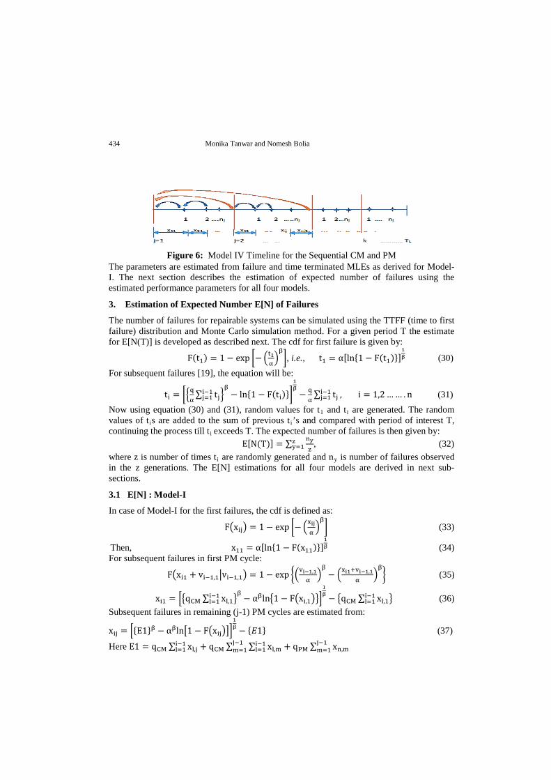
A repairable system with corrective and scheduled preventive maintenances under Model-IV restores the complete operating age since new under PM and restores latest operating age after CM. The Model IV restoration pattern is shown in Figure 6. Virtual age at any ith failure in jth PM interval for Model-II is defined as:

vij = qCM ∑ �xl,j�il=1 + vj−1 (29)

where vj−1 = qPM�qCM ∑ ∑ xl,m𝑛𝑚−1l=1 + ∑ x n𝑚,m

𝑗−1m=1

𝑗−1𝑚=1 �

434 Monika Tanwar and Nomesh Bolia

Figure 6: Model IV Timeline for the Sequential CM and PM

The parameters are estimated from failure and time terminated MLEs as derived for Model-I. The next section describes the estimation of expected number of failures using the estimated performance parameters for all four models.

3. Estimation of Expected Number E[N] of Failures

The number of failures for repairable systems can be simulated using the TTFF (time to first failure) distribution and Monte Carlo simulation method. For a given period T the estimate for E[N(T)] is developed as described next. The cdf for first failure is given by:

F(t1) = 1 − exp �− �t1α�β�, i.e., t1 = α[ln{1 − F(t1)}]

1β (30)

For subsequent failures [19], the equation will be:

ti = ��qα∑ tji−1j=1 �

β− ln{1 − F(ti)}�

1β− q

α∑ tji−1j=1 , i = 1,2 … … . n (31)

Now using equation (30) and (31), random values for t1 and ti are generated. The random values of tis are added to the sum of previous ti’s and compared with period of interest T, continuing the process till ti exceeds T. The expected number of failures is then given by:

E[N(T)] = ∑ nyz

zy=1 , (32)

where z is number of times ti are randomly generated and ny is number of failures observed in the z generations. The E[N] estimations for all four models are derived in next sub-sections.

3.1 E[N] : Model-I

In case of Model-I for the first failures, the cdf is defined as:

F�xij� = 1 − exp �− �xijα�β� (33)

Then, x11 = α[ln{1 − F(x11)}]1β (34)

For subsequent failures in first PM cycle:

F�xi1 + vi−1,1�vi−1,1� = 1 − exp ��vi−1,1α�β− �xi1+vi−1,1

α�β� (35)

xi1 = ��qCM ∑ xl,1i−1l=1 �β − αβln�1 − F�xi,1���

1β − �qCM ∑ xl,1i−1

l=1 � (36) Subsequent failures in remaining (j-1) PM cycles are estimated from:

xij = �{E1}β − αβln�1 − F�xij���1β − {𝐸1} (37)

Here E1 = qCM ∑ xl,j + qCM ∑ ∑ xl,m + qPMi−1l=1

j−1m=1

i−1l=1 ∑ xn,m

j−1m=1

Maintenance Modelling using Generalized Renewal Process for Sequential 435 Imperfect Corrective and Preventive Maintenance

3.2 E[N] : Model-II

The first failure for Model-II are estimated using equation (34) as in case of Model-I. Subsequent failures in first PM cycle are estimated using:

xi1 = ��qCM ∑ qCMi−1xl,1i−1l=1 �β − αβln�1 − F�xi,1���

1β − �qCM ∑ qCMi−1xl,1i−1

l=1 � (38) Subsequent failures in remaining (j-1) PM cycles are given by:

xij = �{E2}β − αβln�1 − F�xij���1β − {E2} (39)

Here E2 = qCM ∑ qCMi−1xl,j + qCMqPM ∑ ∑ qCMn−l−1xl,mn−1l=1

j−1m=1

il=1 + qPMqCM ∑ xn,m

j−1m=1

3.3 E[N] : Model-III

First failures in Model-III are estimated using equation (34), and the subsequent failures in first PM cycle are estimated using equation (36), as described in section 3.1 for Model-I. Subsequent failures in remaining (j-1) PM cycles are then estimated from:

xij = �{E3}β − αβln�1 − F�xij���1β − {E3} (40)

Here E3 = qCM ∑ xl,j + qCMqPM ∑ ∑ qCMn−l−1xl,m + qPMn−1l=1

j−1m=1

i−1l=1 ∑ xn,m

j−1m=1

3.4 E[N] : Model-IV

The first failures for Model-IV are estimated using equation (34) as discussed in section 3.1 for Model-I. Subsequent failures in first PM cycle are estimated as:

xi1 = ��qCM ∑ xl,1i−1l=1 �β − αβln�1 − F�xi,1���

1β − �qCM ∑ xl,1i−1

l=1 � (41) Successive failures in remaining (j-1) PM cycles are given by:

xij = �{E3}β − αβln�1 − F�xij���1β − {E3} (42)

Using equations (34)-(42) the expected number of failures are estimated for all discussed models and are shown in Figures 7-12. The residual MTTF estimation procedure is discussed in next section.

4. Residual Mean Time to Failure

The conditional probability of survival is defined in section 2.1, and presented in Figure 2. A residual MTTF at time t for a repairable system can then be derived using conditional reliability: RMTTF = 1

R(T)∫ R(t′∞T )dt′ (43)

Therefore residual MTTF at virtual age v(t) can be written as: RMTTF = 1

R(v(t))∫ R(t′∞v(t) )dt′ (44)

The next section illustrates this computation for all four models of section 2 and also for Kijima-I and II models.

5. Numerical Illustration

In this section a repairable system failure data with scheduled PM is analyzed in detail for the proposed models. Further the parameters, expected number of failures and residual life are computed for both Kijima-I and II as well as the four proposed virtual age models.

436 Monika Tanwar and Nomesh Bolia

Parameter values for Kijima-I, II and Model-I, II, III, IV are estimated as described in section 2 and corresponding values are summarized in Table 1 and Table 2. In this case the failure data is a real time field failure data on aviation engine for the complete operation of the engine over one overhaul cycle. Since the failure data is taken for one overhaul cycle and rebuilding is assumed after overhaul, there is no requirement for time termination and all performance parameters are estimated and are shown in Table 1 and 2.

Table 1: Kijima I and Kijima II Virtual Age Model Parameters

Model α β q KI (Engine) 512.05 1.35 0.75

KII (FM) 430.15 1.62 1.11 KI (FM) 410.42 1.46 0.85

Table 2: Model-I, II, III Virtual Age Parameters

Model α β qCM qPM Model I 512.05 1.35 1.1 0.60 Model II 545.03 1.37 1.40 0.70 Model III 510.07 1.32 1.90 0.74 Model IV 513.15 1.31 2.10 0.80

The expected number of failures is estimated for the proposed models as well as Kijima Models. Figure 7 presents the actual failures and expected number of failures for Model I, Model II and KI. It is evident from the plot that Model-I has comparatively better fit to the original data than KI.

Figure 7: Expected Number of Failures vs. Operating Time for Model-I, II and K-II

The expected number of failures of Model–II presented in Figure 7 has a huge difference in observed failure points and expected number of failures. The cause of this difference in case of Model-II is further analyzed. For Model-II it is assumed that both CM and PM at any point of time completely restore the operating age since new. In this case, the repairable engine data has multiple FMs with CM and PM. Therefore, a specific repair action for a FM may not be able to restore other FM, thus leading to a poor fit in Figure 7. To test this further, following is done: Since the engine data has several FMs, and a specific repair action for a FM may not be able to restore other FM, the data for a specific FM is analyzed. The K-II MLEs are then used to estimate expected number of failures for a specific FM having no PM.

The values of performance parameters are shown in Table 1 and the estimated expected number of failures for both KII and KI are plotted against operating hours and presented in Figures 8 and 9. This particular FM has shown comparatively better fit to KII rather than multiple failure modes of an engine under Model-II. The comparison of Model-II and K-II is made possible on the basis of the common concept of virtual age. As expected it is observed that if failure data is fitting to KII then it also fits to K-I whereas vice versa is not

0

20

40

60

80

0 5 0 1 0 0 1 5 0 2 0 0 2 5 0 3 0 0 3 5 0 4 0 0 4 5 0 5 0 0 5 5 0

FAIL

URE

S

TIME (HRS)

DATA MODEL IKIJIMA I MODEL II

Maintenance Modelling using Generalized Renewal Process for Sequential 437 Imperfect Corrective and Preventive Maintenance

possible (as in case of Model I and Model-II).The analysis is continued using K-I for FM data and the results are tabulated in Table 1 and presented in Figure 9. However, goodness of fit estimation can prove to be a better way to find the best model fit for the data, and it is still an area open for research [20], [21], [22]. Model-III has different restoration pattern for both CM and PM, as CM l restores the latest operating age whereas PM restores the time since new. Figure 10 and 11 show the estimated expected number of failures for Model-III, and Model IV in comparison with KI model respectively. It is evident from Figure that estimated failures using the models suggested in this paper provide better fit to observed failure data than KI model. The performance parameters like virtual age, residual MTTF and system availability are estimated for Model I, III, IV and KI, results are then plotted, and corresponding effect of PM is evident from Figures 12-14.

Figure 8: Expected Number of Failures vs. Operating Time under K-II for

Single Failure Mode

Figure 9: Expected Number of Failures vs. Operating Time under K-I for

Single Failure Mode

Figure 10: Expected Number of Failures vs. Operating Time for Model-III and

K-I

-50

0

50

100

50 100 150 200 250 300 350 400 450 500FAIL

URE

S

TIME(HRS)

KII-FMDATA

-50

0

50

100

50 100 150 200 250 300 350 400 450 500FAIL

URE

S

TIME(HRS)

KI-FM

DATA

0

20

40

60

80

0 50 100 150 200 250 300 350 400 450 500 550

FAIL

URE

S

TIME (HRS)

DATAMODEL IIIK-I

438 Monika Tanwar and Nomesh Bolia

Figure 11: Expected Number of Failures vs. Operating Time for Model-IV and K-I

Figure 12: Virtual Age vs. Operating Time for Models I, III, IV and KI

Figure 13: Virtual Age vs. Operating Time for Model II

Figure 14: Residual MTTF vs. Operating Time for Model-I, II, III, IV and KI

From Table 3 it is observed that the qPM is less than the qCM indicating requirement for improvement in CM actions and responsible for higher virtual age, whereas the KI repair

0

20

40

60

80

0 50 100 150 200 250 300 350 400 450 500 550

FAIL

URE

S

TIME (HRS)

DATAMODEL IVK-I

0

500

1000

14 50 84 102

150

162

200

213

257

300

324

338

350

380

446

494

522

541

549

VIRT

UAL

AG

E

TIME (HRS)

Model IMODEL IIIModel IVK I

0

20000

VIRT

UAL

AG

E

TIME (HRS)

Model-II

0.00

200.00

400.00

14 50 84 102

150

162

200

213

257

300

324

338

350

380

446

494

522

541

549

RESI

DUAL

MTT

F

TIME (HRS)

Model IModel IIModel IIIModel IVK I

Maintenance Modelling using Generalized Renewal Process for Sequential 439 Imperfect Corrective and Preventive Maintenance

effectiveness gives single estimate for imperfection in maintenance and may lead to error in repair improvement decision for both CM and PM. The comparison of KI and Model I provides the difference in parameter estimates following the same restoration pattern. From Fig. 6 the Model I fitness is found better to the failure data than KI. Therefore the estimation of both indices of repair effectiveness is found more appropriate than single repair effectiveness index estimation. The proposed models can further be used for various PM and CM after repair states:

Table 3: Various Combinations of PM and CM S. No. Possible Cases qPM qcM

1. Imperfect CM and No PM NIL # 2. Imperfect CM and Minimal PM 1 # 3. Imperfect CM and Perfect PM 0 # 4. Minimal CM and Perfect PM 0 1 5. Minimal CM and Imperfect PM 1 0 6. Minimal CM and Minimal PM 1 1 7. Imperfect CM and Imperfect PM # # 8. Perfect CM and imperfect PM # 0 9. Minimal PM and Perfect CM 1 0

NOTE: # represents possibility of any of five after repair states i.e., ‘AGAN’, ‘ABAO’, ‘BOWN, ‘WTO’, and ‘BTN’.

6. Conclusion

Existing models for repairable system analysis consider two restoration patterns i.e., restoration of latest operating age after recent failure and operating age since new, using single and constant repair effectiveness index. In practice however there are possibilities of other restoration patterns, and it is also observed that the use of single repair effectiveness is not appropriate where sequential CM and PM takes place. In this paper, the virtual ages are modeled with sequential repair effectiveness indices for both CM and PM considering four different restoration patterns. The paper then brings out the methodology for providing MLEs of all the performance parameters by two different methods. The first method of obtaining MLEs is by modeling the likelihood function as constraint optimization problem. The second method is by providing derivatives for directly obtaining the MLEs. The paper also provides a methodology for estimating residual life for imperfect repairs. The expected number of failures for the proposed approaches is also estimated using Monte Carlo simulation. A comparative analysis is provided to get insight of better fit for the proposed models.

Acknowledgement: Authors are thankful to the MHRD, India for supporting this research work and to a referee and Editor-in-Chief for improving upon the original paper.

References [1] Nakagawa, T. Imperfect Preventive Maintenance. IEEE Transactions on Reliability. 1978; R-

28(5): 9529. [2] Nakagawa, T. Optimum Policies When Preventive Maintenance Is Imperfect. IEEE Transactions

on Relaibility, 1979; R-28(4): 331–332. [3] Brown, M. and F.Proschan. Imperfect Repair. Journal of Applied Probability, 1983; 20(4): 851–

859. [4] Block, H.W., W.S. Borges, and T.H. Savits. Age Dependent Minimal Repair. Journal of Applied

Probability,1985; 22(2): 370–385.

440 Monika Tanwar and Nomesh Bolia

[5] Kijima, M. and U. Sumita. A Useful Generalization of Renewal Theory Counitng Processes Governed by Non-Negative Markovian Increments. Journal of Applied Probability. 1986; 23(1): 71–88.

[6] Kijima, M. Some Results for Repairable Systems with General Repair. Journal of Applied Probability, 1989; 26(1): 89–102.

[7] Dijoux, Y. A Virtual Age Model based on A Bathtub Shaped Initial Intensity. Reliability Engineering & System Safety, 2009; 94(5): 982–989.

[8] Doyen, L. and O. Gaudoin. Classes of Imperfect Repair Models based on Reduction of Failure Intensity or Virtual Age. Relaibility Engineering and System Safety, 2004; 84(1): 45-46.

[9] Kijima, M., H. Morimura, and Y. Suzuki. Periodical Replacement Problem Without Assuming Minimal Repair. European Journal of Operational Research, 1988; 37(2): 194-203.

[10] Jack, N. Age-reduction Models for Imperfect Maintenance. IMA Journal of Mathematics Applied in Buisness & Industry, 1998; 9(4): 347–354.

[11] Doyen, L. and O. Gaudoin. Modelling and Assessment of Aging and Efficiency of Corrective and Planned Preventive Maintenance Maintenance. IEEE Transactions on Reliability, 2011; 60(4): 759-69.

[12] Ramirez, P. A. P. and I. B. Utne. Decision Support for Life Extension of Technical Systems through Virtual Age Modelling. Relaibility Engineering and System Safety, 2013; 115: 55-69.

[13] Hurtado, J. L., Joglar, F. and Modarres, M. Generalized Renewal Process: Models, Parameter Estimation and Applications to Maintenance Problems. International Journal of Performability Engineering, 2005; 1(1): 37-50.

[14] Liu, X. G. , V. Makis and A. K. S. Jardine. A Replacement Model with Overhauls and Repairs. Naval Research Logistics, 1995; 42(7): 1063-1079.

[15] Pham, H. and H. Wang. Imperfect Maintenance. European Journal of Operational Research, 1996; 94(3): 425-438.

[16] Tanwar, M., R. N. Rai, N. Bolia. Imperfect Repair Modeling using Kijima Type Generalized Renewal Process. Relaibility Engineering and System Safety, 2014; 124: 24-31.

[17] Mettas, A. and W. Zhao. Modeling and Analysis of Repairable Systems with Genearl Repair. Proceedings of IEEE Annual Reliability and Maintainability Symposium. Alexandria, Virginia, USA, 2005.

[18] Yañez, M., F. Joglar, and M. Modarres. Generalized Renewal Process for Analysis of Repairable Systems with Limited Failure Experience. Reliability Engineering & System Safety, 2002; 77(2): 167–180.

[19] Fuqing, Y. and U. Kumar. Time-Dependent Repair Effectiveness. IEEE Transactions on Reliability, 2012; 61(1): 95–100.

[20] Park, W. J. and M. Ieee. More Goodness-of-Fit Tests for the Power-Law Process. IEEE Transactions on Reliability, 1994; 43(2): 275–278.

[21] Gaudoin, O., B. Yang, M. Xie, and S. Member. A Simple Goodness-of-Fit Test for the Power-Law Process , based on the Duane Plot. IEEE Transactions on Reliability, 2003; 52(1): 69–74.

[22] Liu, Y., H. Huang, and X. Zhang. A Data-Driven Approach to Selecting Imperfect Maintenance Models. IEEE Transactions on Reliability, 2012; 61(1): 101–112.

Monika Tanwar received the B.E. degree in Mechanical Engineering from Rajasthan University, India, in 2006 and M. Tech. Degree in Industrial Tribology and Maintenance Engineering from Indian Institute of Technology Delhi, India in 2011. She has submitted her Ph.D. dissertation in Department of Mechanical Engineering at Indian Institute of Technology Delhi, India. Her research interests are repairable system maintenance modelling, human error analysis, inventory management, imperfect maintenance, maintenance performance and reliability analysis.

Nomesh Bolia completed his Ph.D. in Operations Research from University of North Carolina at Chapel Hill. He is currently a faculty member in the department of

Maintenance Modelling using Generalized Renewal Process for Sequential 441 Imperfect Corrective and Preventive Maintenance

Mechanical Engineering at the Indian Institute of Technology Delhi. He has several sponsored research projects from public funding agencies such as DST/HUDCO as well as research labs of companies such as GE/Philips and consults for public/private sector companies such as JCB India and Rajasthan State Mines and Minerals Ltd.

Appendix A

Note: In Appendix A and B, if we define a=q∑ qn−jxji−1j1 , then:

∂[ln(L)]∂α

= βαβ+1

× ∑ �(qxi + a)β − (a)β� + βα

ni=2 ��x1

α�β− n� = 0 (A1)

∂[ln(L)]∂β

= �nβ

+ ln(x1) − nlnα − �x1α�β

ln �x1α��+ ∑ �

ln(qxi + a) − �qxi+aα�β

ln �qxi+aα� + �a

α�β

ln �a� = 0n

i=2 (A2)

∂[ln(L)]∂q

= (β − 1)∑ �xi+∑ (n−j+1)q(n−j)xji−1

j=1

qxi+a�n

i=2 + βq(β−1)

αβ∑ �xi + ∑ (n − j + 1)q(n−j)xji−1

j=1 �βn

i=2 −βαβ∑ (qxi + a)β−1�xi + ∑ (n − j + 1)q(n−j)xji−1

j=1 � = 0 ni=2 (A3)

Appendix B

∂[ln(L)]∂α

= βαβ+1

�∑ (qxi + a)βni=2 − (a)β� + β

�x1

α�β− n� + β

α�qxi+a

α�β− β

α= 0 (B1)

∂[ln(L)]∂β

= �nβ

+ ln(x1) − nlnα − �x1α�β

ln �x1α��+ ∑ �ln�qxi + q∑ qn−jxji−1

j=1 � − �qxi+aα�β

×ni=2

ln �qxi+aα� + �a

α�β

ln �aα�� − �a

α�β

ln �aα� + �a

α� ln �a

α� = 0 (B2)

∂[ln(L)]∂q

= (β − 1)∑ �xi+∑ (n−j+1)q(n−j)xji−1

j=1

qxi+q∑ qn−jxji−1j=1

� + βqβ−1

αβni=1 ∑ �∑ xji−1

j=0 �β− β

αβni=1 × �∑ �qxi +n

i=1

q∑ qn−jxji−1j=0 �

β−1�q∑ qn−jxji−1

j=0 ��+ βα�aα� − β �qxi+a

α�β

× �xi+∑ (n−j+1)q(n−j)xjn

j=1

qX+a� = 0 (B3)

Appendix C

Note: Let us define b = �xij + qCM ∑ xl,ji−1l=1 + qCM ∑ ∑ xl,mi−1

l=1j−1m=1 + qPM ∑ xnj,m

j−1m=1 �

and b′ = qCM ∑ xl,ji−1l=1 + qCM ∑ ∑ xl,mi−1

l=1j−1m=1 + qPM ∑ xn,m

j−1m=1 , then, we have:

∂[ln(L)]∂α

= βαβ+1

�(x11)β + ∑ �xi1 + qCM ∑ xl,1i−1l=1 �

βn1i=2 − �qCM ∑ xl,1i−1

l=1 �β� + ∑ ∑ �𝑏β −nj

i=1kj=2

�b − xij�β� + β

α�k − njk − 2� = 0 (C1)

∂[ln(L)]∂β

=

�ln �x11α� × �1 − �x11

α�β��+ ∑ �ln�xi1 + qCM ∑ xl,1i−1

l=1 � + ��qCM∑ xl,1i−1l=1α

�β

× ln �qCM∑ xl,1i−1l=1α

�� −n1i=2

��xi1+qCM∑ xl,1i−1l=1

α�β

× ln �xi1+qCM∑ xl,1i−1l=1

α���∑ ∑ �lnb + ��b1

α�β

× ln �b1α�� − ��b

α�β

× ln �bα���nj

i=1kj=2 +

�njk−k−2β

� − ��nj − 1�(k− 1)nj ln α� = 0 (C2) ∂[ln(L)]∂qCM

=

�(𝛽 − 1)∑ � ∑ 𝑥𝑙,1𝑖−1𝑙=1

𝑥𝑙,1+qCM∑ 𝑥𝑙,1𝑖−1𝑙=1

�𝑛1𝑖=2 + 𝛽𝑞𝐶𝐶

𝛽−1

𝛼𝛽∑ �∑ 𝑥𝑙,1𝑖−1

𝑙=1 �𝑛1𝑖=2 −

442 Monika Tanwar and Nomesh Bolia

𝛽𝛼∑ �𝑥𝑙,1 + qCM ∑ 𝑥𝑙,1𝑖−1

𝑙=1 �𝛽−1�qCM ∑ 𝑥𝑙,1𝑖−1𝑙=1 �𝑛1

𝑖=2 � + ∑ ∑ ��(𝛽−1)�∑ 𝑥𝑙,𝑗𝑖−1

𝑙=1 +∑ ∑ 𝑥𝑙,𝑚𝑖−1𝑙=1

𝑗−1𝑚=1 �

b� +𝑛𝑗

𝑖=1𝑘𝑗=2

��∑ 𝑥𝑙,𝑗𝑖−1𝑙=1 + ∑ ∑ 𝑥𝑙,𝑚𝑖−1

𝑙=1𝑗−1𝑚=1 �

𝛽× 𝛽

𝛼𝛽× �b − xij�

𝛽−1� −

� 𝛽𝛼𝛽

(b)𝛽−1 × �∑ 𝑥𝑙,𝑗𝑖−1𝑙=1 + ∑ ∑ 𝑥𝑙,𝑚𝑖−1

𝑙=1𝑗−1𝑚=1 ��� = 0 , (C3)

and ∂[ln(L)]∂qPM

= ∑ ∑ ��(β−1)�xn,j−1�

(𝑏) � + �xnj,j−1� �βαβ� ��b − xij�

β−1 − (b)β−1��ni=1

kj=2 = 0 (C4)