Embed Size (px)
Citation preview

Field Monitoring for LULUCF Projects
Winrock International
Training Seminar for BioCarbon Fund Projects
IPCC GPG Chapter 4.3 Provides good practice guidance
for JI and CDM projects and includes guidance on:• defining project boundaries, • measuring, monitoring, and
estimating changes in carbon stocks and non-CO2 greenhouse gases,
• implementing plans to measure and monitor,
• developing quality assurance and quality control plans
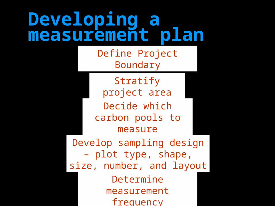
Developing a measurement planDefine Project Boundary
Stratify project area
Decide which carbon pools to measure
Develop sampling design – plot type, shape, size, number, and layout
Determine measurement frequency
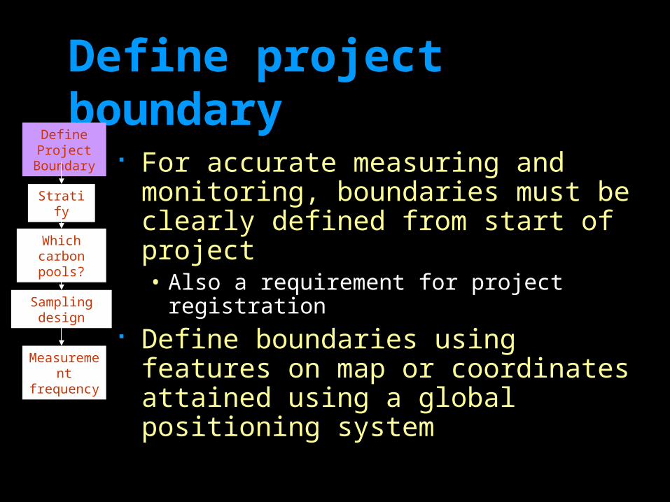
For accurate measuring and monitoring, boundaries must be clearly defined from start of project• Also a requirement for project
registration Define boundaries using features
on map or coordinates attained using a global positioning system
Define project boundaryDefine Project
Boundary
Stratify
Which carbon pools?
Sampling design
Measurement frequency

Project can vary in size: 10’s ha 1000’s ha
Project can be one contiguous block OR many small blocks of land spread over a wide area
One OR many landowners
Define project boundaryDefine Project
Boundary
Stratify
Which carbon pools?
Sampling design
Measurement frequency
Carbon sampling Methods for measuring carbon credits
are based on measuring changes in carbon stocks
Not practical to measure everything - so we sample
Sample subset of land by taking relevant measurements of selected pool components in plots
Number of plots measured predetermined to ensure both accuracy and precision
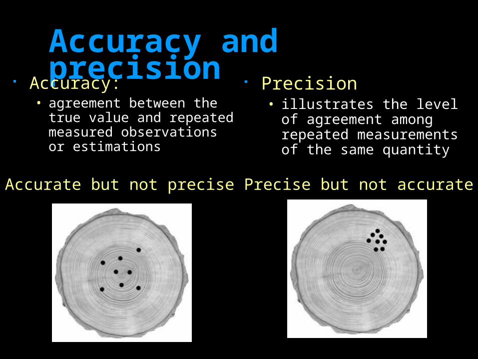
Accuracy and precision Accuracy:
• agreement between the true value and repeated measured observations or estimations
Precision• illustrates the level of
agreement among repeated measurements of the same quantity
Accurate but not precise Precise but not accurate

Principles of monitoring carbon There is a trade-off between the desired
precision level of carbon-stock estimates and cost
In general, the costs will increase with: • Greater spatial variability of the carbon
stocks• The number of pools that need to be
monitored • Precision level that is targeted• Frequency of monitoring• Complexity of monitoring methods
Stratification of the project lands into a number of relatively homogeneous units can reduce the number of plots needed.
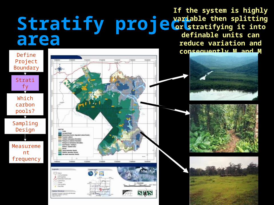
Stratify project areaIf the system is highly
variable then splitting or stratifying it into
definable units can reduce variation and
consequently M and M costs
Define Project Boundary
Stratify
Which carbon pools?
Sampling Design
Measurement frequency
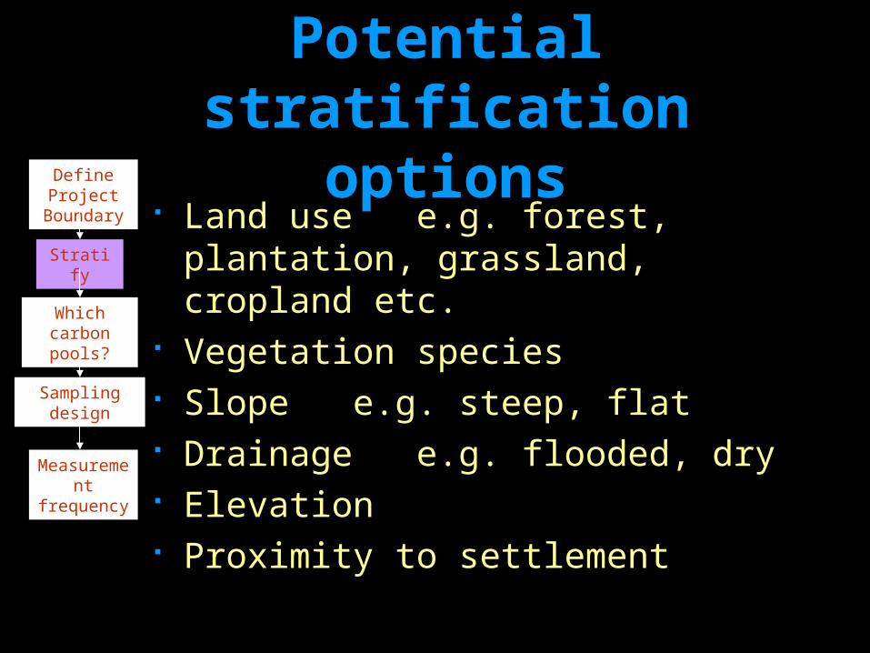
Land use e.g. forest, plantation, grassland, cropland etc.
Vegetation species Slope e.g. steep, flat Drainage e.g. flooded, dry Elevation Proximity to settlement
Potential stratification optionsDefine Project
Boundary
Stratify
Which carbon pools?
Sampling design
Measurement frequency
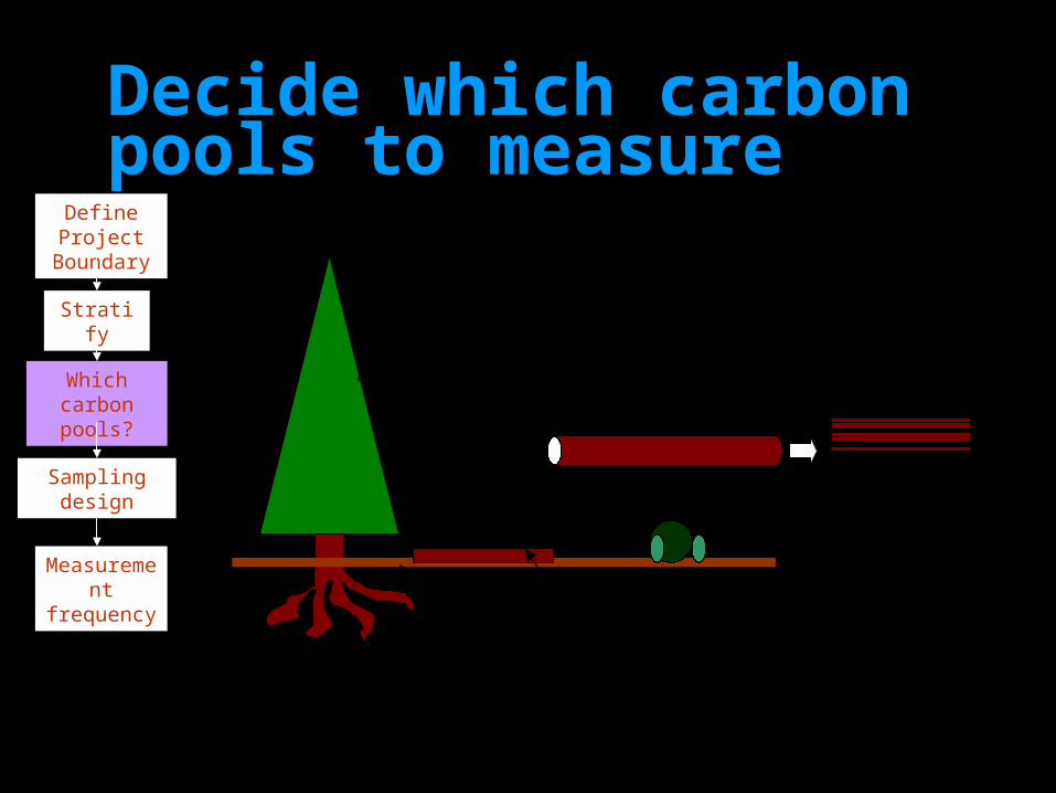
Decide which carbon pools to measure
Define Project Boundary
Stratify
Which carbon pools?
Sampling design
Measurement frequency
Soil Carbon
Herbaceous vegetation
Wood products
Branches
Litter
Dead wood
Roots
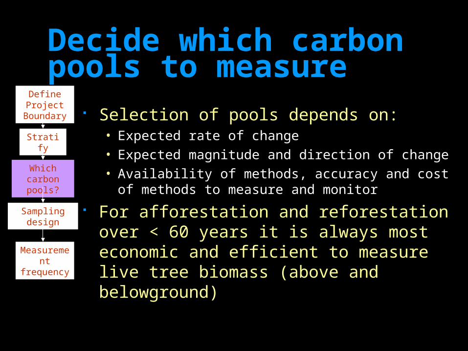
Selection of pools depends on:• Expected rate of change• Expected magnitude and direction of change• Availability of methods, accuracy and cost of
methods to measure and monitor For afforestation and reforestation
over < 60 years it is always most economic and efficient to measure live tree biomass (above and belowground)
Decide which carbon pools to measure
Define Project Boundary
Stratify
Which carbon pools?
Sampling design
Measurement frequency
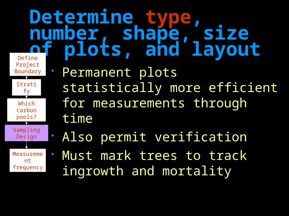
Determine type, number, shape, size of plots, and layout
Permanent plots statistically more efficient for measurements through time
Also permit verification Must mark trees to track
ingrowth and mortality
Define Project Boundary
Stratify
Which carbon pools?
Sampling Design
Measurement frequency
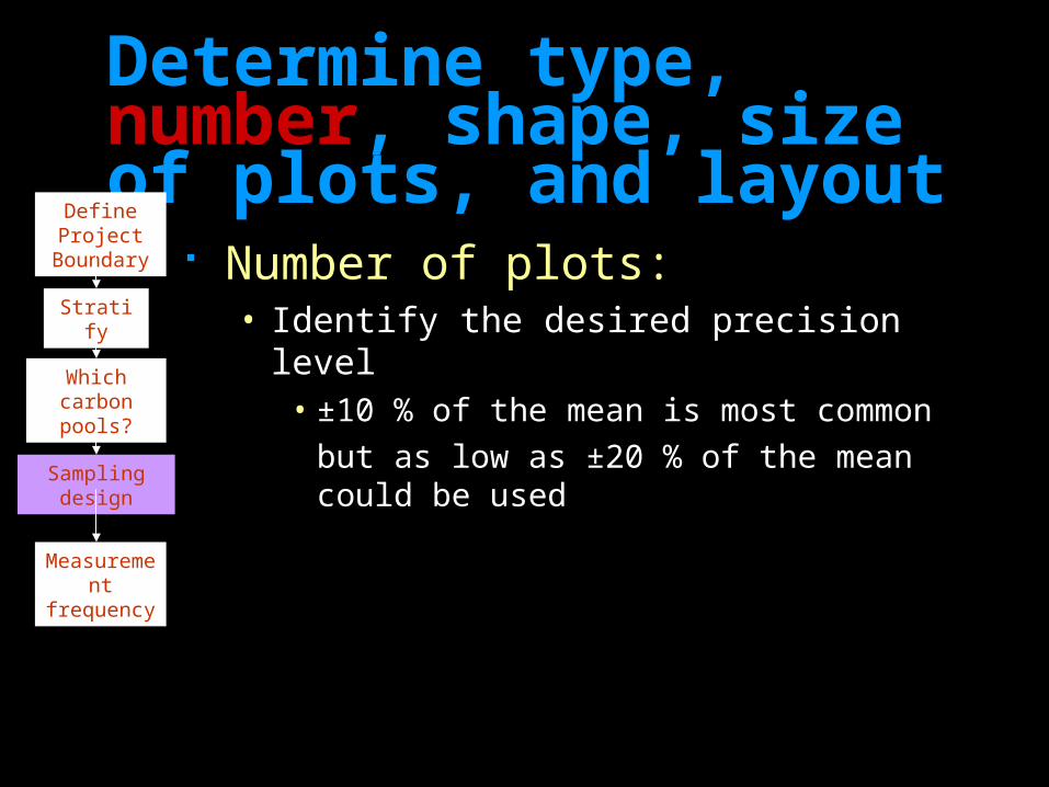
Number of plots:• Identify the desired precision level
• ±10 % of the mean is most commonbut as low as ±20 % of the mean could be used
Determine type, number, shape, size of plots, and layout
Define Project Boundary
Stratify
Which carbon pools?
Sampling design
Measurement frequency
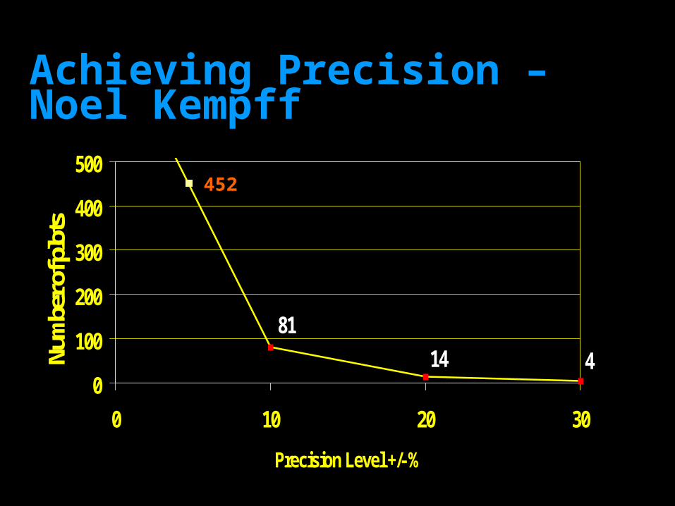
Achieving Precision – Noel Kempff
81
14 40
100
200
300
400
500
0 10 20 30
Precision Level +/- %
Num
ber o
f plo
ts
452
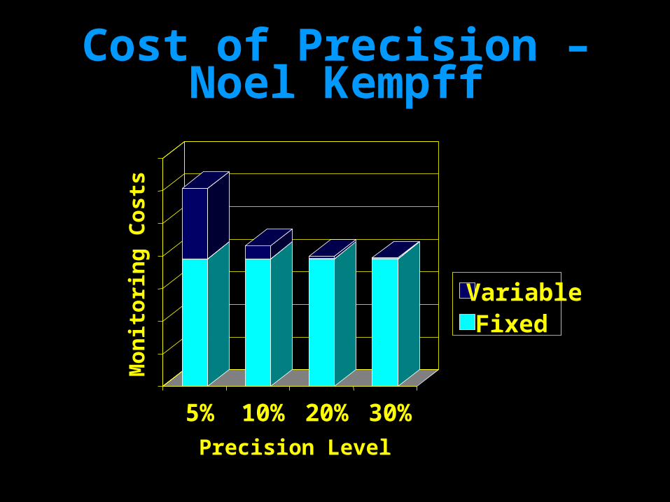
Cost of Precision – Noel Kempff
Mon
itorin
g C
osts
5% 10% 20% 30%Precision Level
VariableFixed
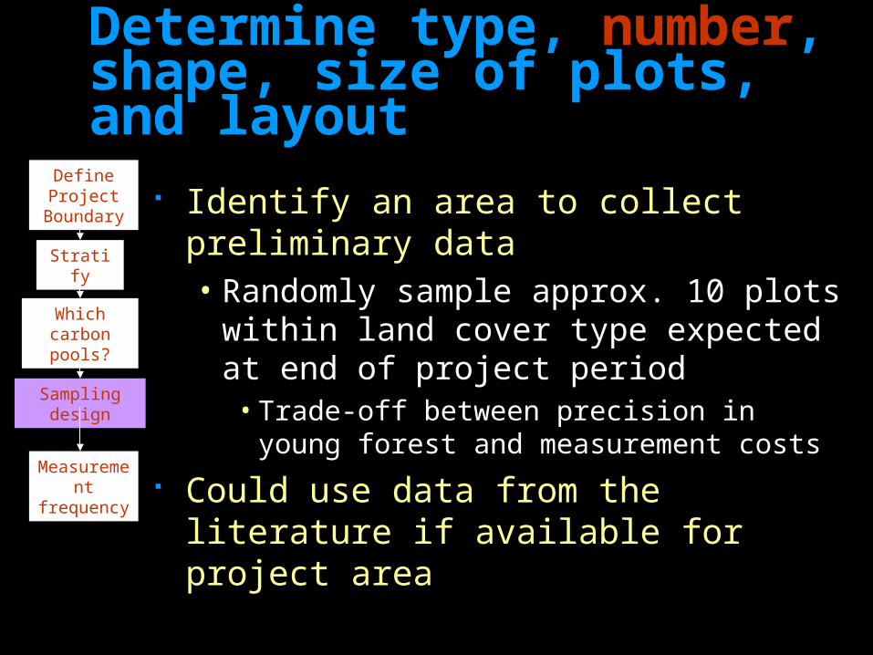
Identify an area to collect preliminary data • Randomly sample approx. 10 plots
within land cover type expected at end of project period• Trade-off between precision in young
forest and measurement costs Could use data from the literature
if available for project area
Determine type, number, shape, size of plots, and layout
Define Project Boundary
Stratify
Which carbon pools?
Sampling design
Measurement frequency
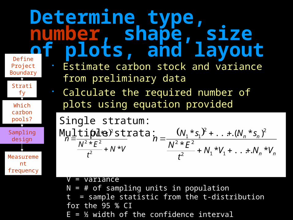
Single stratum: Multiple strata:
Determine type, number, shape, size of plots, and layout
VN
tEN
sNn
**
*
2
22
2
nn
nn
VNVNt
ENsNsN
n*.....*
*)*(.....*
112
22
2211
s = standard deviationV = varianceN = # of sampling units in populationt = sample statistic from the t-distribution for the 95 % CIE = ½ width of the confidence interval
Define Project Boundary
Stratify
Which carbon pools?
Sampling design
Measurement frequency
Estimate carbon stock and variance from preliminary data
Calculate the required number of plots using equation provided
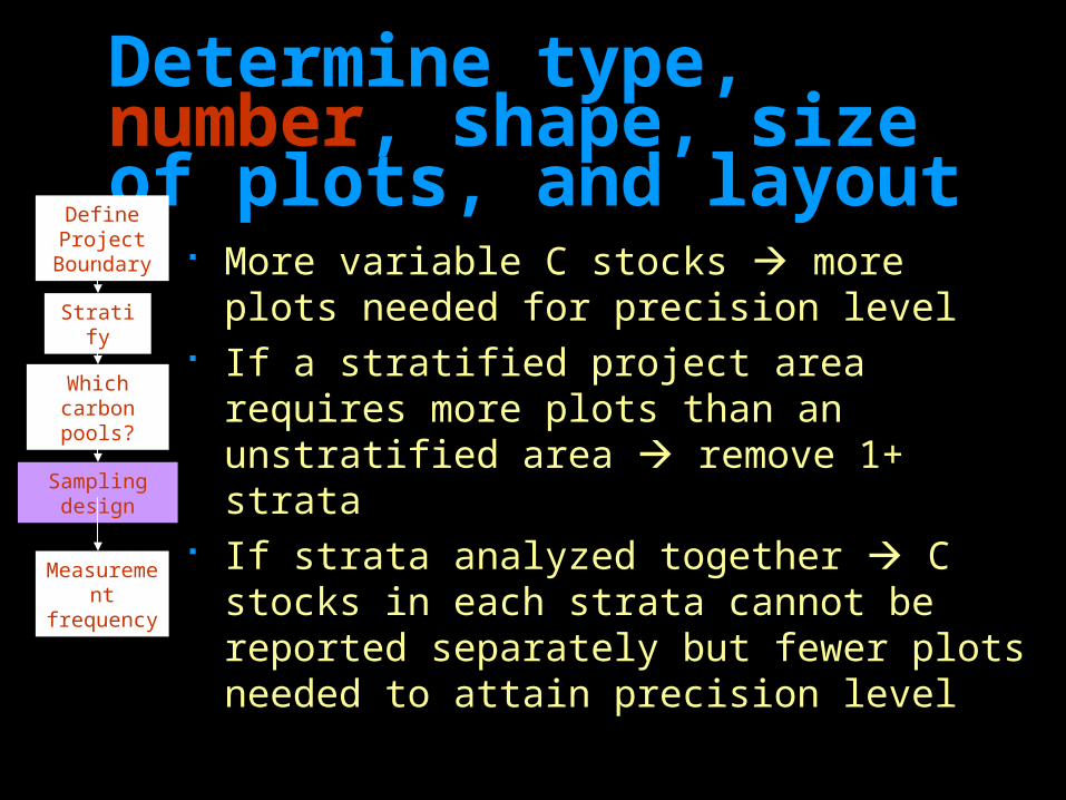
More variable C stocks more plots needed for precision level
If a stratified project area requires more plots than an unstratified area remove 1+ strata
If strata analyzed together C stocks in each strata cannot be reported separately but fewer plots needed to attain precision level
Determine type, number, shape, size of plots, and layout
Define Project Boundary
Stratify
Which carbon pools?
Sampling design
Measurement frequency
Non-tree carbon pool:• Above method can be used• However, size of non-tree carbon pool most
likely small in reforestation/afforestation project
• Alternatively, measure non-tree pools in proportion to # tree plots
For example:• For every tree plot, sample:
• Single 100 m line transect for dead wood• 4 sub-plots for herbaceous, forest floor, soil
• May result in large variance, but overall amount small in comparison to tree carbon stock
Determine type, number, shape, size of plots, and layout
Define Project Boundary
Stratify
Which carbon pools?
Sampling design
Measurement frequency
Determine type, number, shape, size of plots, and layout
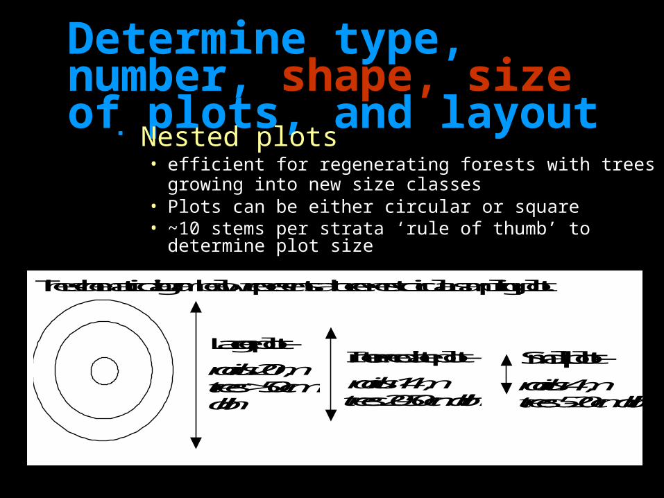
Nested plots • efficient for regenerating forests with trees
growing into new size classes • Plots can be either circular or square• ~10 stems per strata ‘rule of thumb’ to determine
plot size
The schematic diagram below represents a three-nest circular sampling plot.
Large plot –
radius 20 m, trees > 50 cm dbh
Intermediate plot –
radius 14 m, trees 20-50 cm dbh
Small plot –
radius 4 m, trees 5-20 cm dbh
Determine type, number, shape, size of plots, and layout
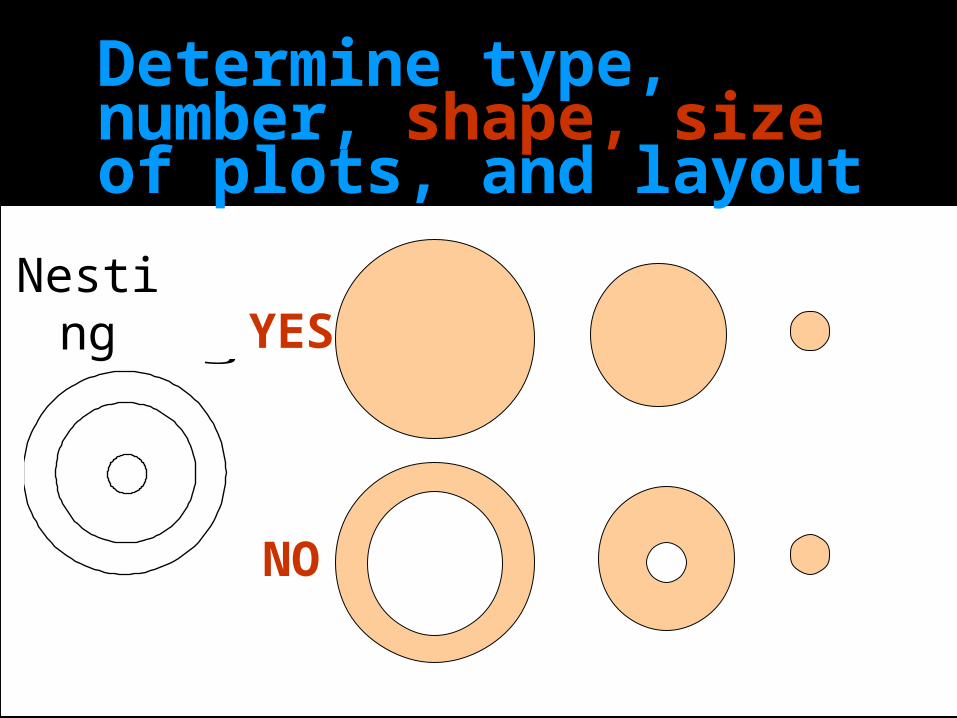
The schematic diagram below represents a three-nest circular sampling plot.
NO
YESNesting
Where an even-age distribution of trees can be expected single plots can be used instead of nested plots
The size of a single plot is a trade-off between adequately sampling large trees late in the project and high effort and cost for sampling small trees initially• This trade-off is avoided with nested
plots
Determine type, number, shape, size of plots, and layout
Define Project Boundary
Stratify
Which carbon pools?
Sampling design
Measurement frequency

Decide if plots to be distributed:• Systematically
• Overlay grid on map• Allocate plots in regular pattern across
strata
• Randomly• Generate random number for bearing and
distance for each plot or randomly allocate in GIS
• Post-stratify• Where highly variable but difficult to stratify
Determine type, number, shape, size of plots, and layout
Define Project Boundary
Stratify
Which carbon pools?
Sampling design
Measurement frequency
Frequency of measurement
For CDM, verification and certification must occur every five years
It is therefore logical to re-measure at this time
However, for slowly changing pools such as soil it will be necessary to measure less frequently
Define Project Boundary
Stratify
Which carbon pools?
Sampling design
Measurement frequency
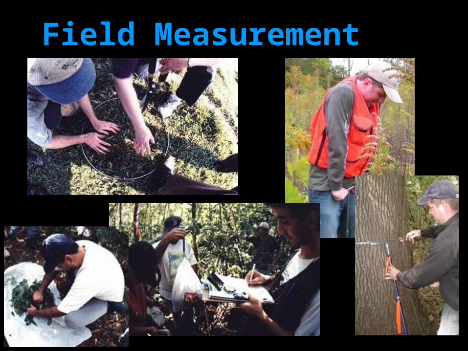
Field Measurement Techniques

Carbon is generally taken to be equal to: ½ Biomass
Alternatively, the proportion of carbon contained in a biomass pool can be measured on a project by project basis
The proportion of carbon in soil will not be 50 % and if soil monitored proportion will need be measured
Carbon versus Biomass
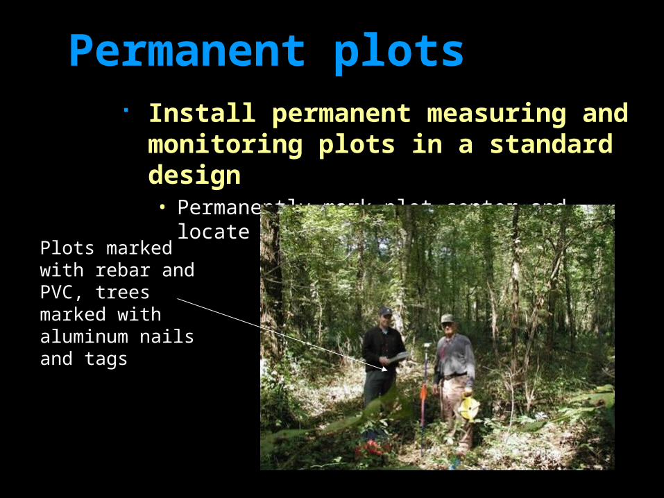
Permanent plots Install permanent measuring and
monitoring plots in a standard design• Permanently mark plot center and locate with
a GPSPlots marked with rebar and PVC, trees marked with aluminum nails and tags
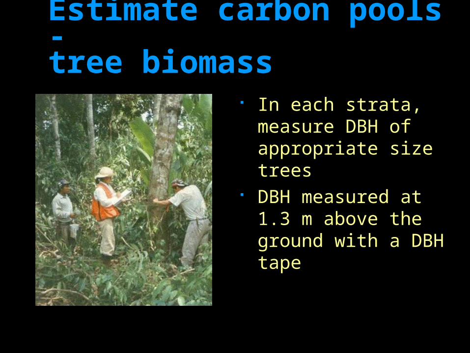
Estimate carbon pools - tree biomass
In each strata, measure DBH of appropriate size trees
DBH measured at 1.3 m above the ground with a DBH tape
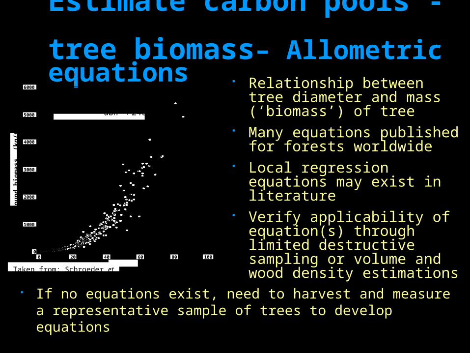
Estimate carbon pools - tree biomass– Allometric equations
Relationship between tree diameter and mass (‘biomass’) of tree
Many equations published for forests worldwide
Local regression equations may exist in literature
Verify applicability of equation(s) through limited destructive sampling or volume and wood density estimations
1008060402000
1000
2000
3000
4000
5000
6000
Ab
oveg
rou
nd
bio
mass
(kg
/tre
e)
Diameter (cm)Taken from: Schroeder et al 1997
If no equations exist, need to harvest and measure a representative sample of trees to develop equations
872,246
000,25 0.5
52
52
.
.
dbh
dbhBiomass
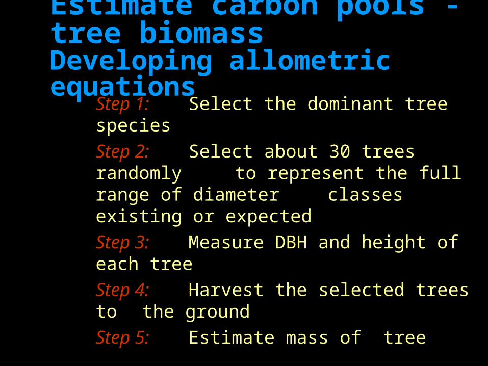
Estimate carbon pools - tree biomass Developing allometric equations
Step 1: Select the dominant tree species
Step 2: Select about 30 trees randomly to represent the full range of
diameter classes existing or expectedStep 3: Measure DBH and height of
each treeStep 4: Harvest the selected trees to
the groundStep 5: Estimate mass of tree
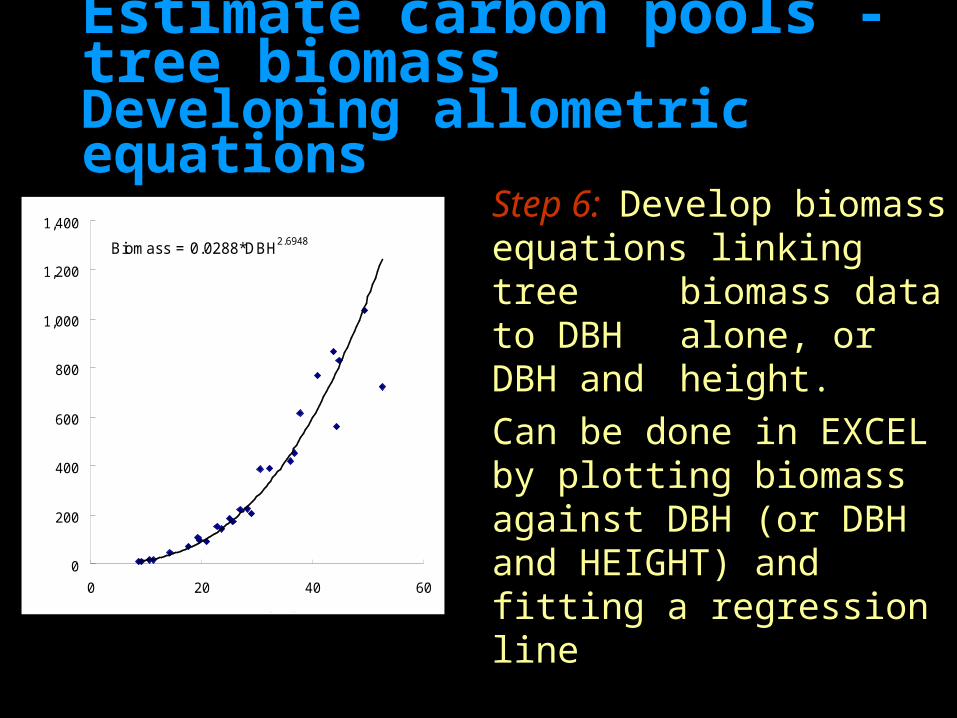
Estimate carbon pools - tree biomass Developing allometric equations
Step 6: Develop biomass equations linking tree biomass data to DBH alone, or DBH and height.Can be done in EXCEL by plotting biomass against DBH (or DBH
and HEIGHT) and fitting a regression
line
Biomass = 0.0288*DBH2.6948
0
200
400
600
800
1,000
1,200
1,400
0 20 40 60DBH (cm)
Bio
ma
ss (
kg C
pe
r tr
ee
)
R2 = 0.98
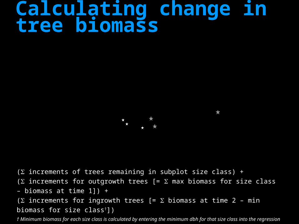
Calculating change in tree biomass
Trees: 001, 002, 003, 004, 005
Trees: 006, 007, 008, 009
Tree: 010
Time 1
Time 2
Trees: 001, 002, 003, 101, 102 Trees: 006,
007, 004, 005, 103 Trees: 010,
009
( increments of trees remaining in subplot size class) +
( increments for outgrowth trees [= max biomass for size class – biomass at time 1]) +
( increments for ingrowth trees [= biomass at time 2 – min biomass for size class†])† Minimum biomass for each size class is calculated by entering the minimum dbh for that size class into the regression
equation (5 cm for the small plot, 20 cm for the intermediate plot and 70 cm for the large plot)

Estimate carbon pools –Dead wood
Dead wood can be a significant component of biomass pools• Particularly in mature
forests – not eligible in first reporting period
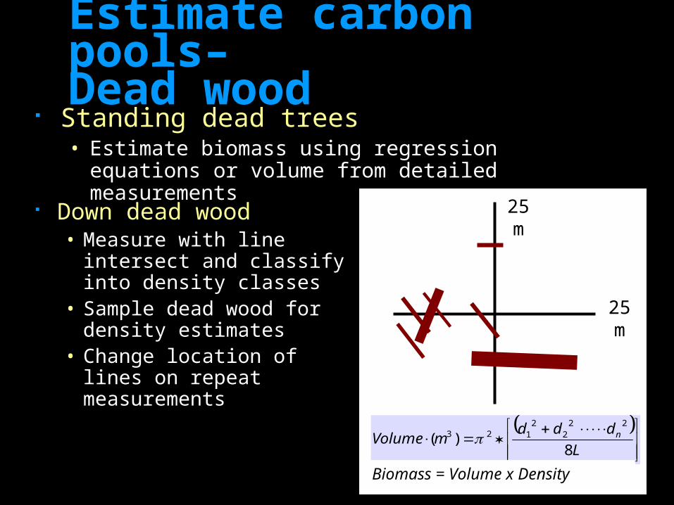
Estimate carbon pools– Dead wood
Standing dead trees• Estimate biomass using regression equations
or volume from detailed measurements
25 m
25 m
L
dddmVolume n
8)(
222
2123
Biomass = Volume x Density
Down dead wood• Measure with line
intersect and classify into density classes
• Sample dead wood for density estimates
• Change location of lines on repeat measurements
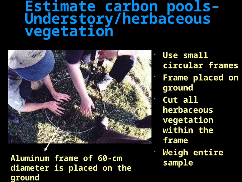
Estimate carbon pools–Understory/herbaceous vegetation
Use small circular frames
Frame placed on ground
Cut all herbaceous vegetation within the frame
Weigh entire sample
Photo by Warwick Manfredi
Aluminum frame of 60-cm diameter is placed on the ground
Estimate carbon pools–Understory/herbaceous vegetation
Collect a sub-sample for moisture determination
Place sub-sample in bag and weigh it
Repeat the process for litter Sub-samples dried and weighed for
determination of dry biomass Place in new location on repeat
measurements
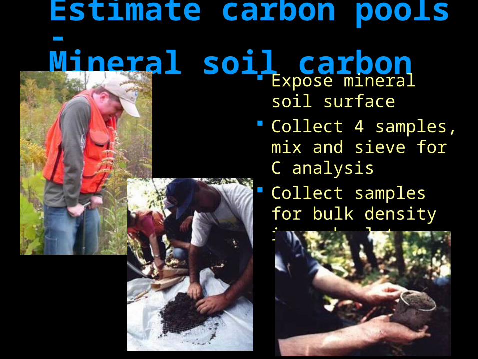
Estimate carbon pools - Mineral soil carbon
Expose mineral soil surface
Collect 4 samples, mix and sieve for C analysis
Collect samples for bulk density in each plot
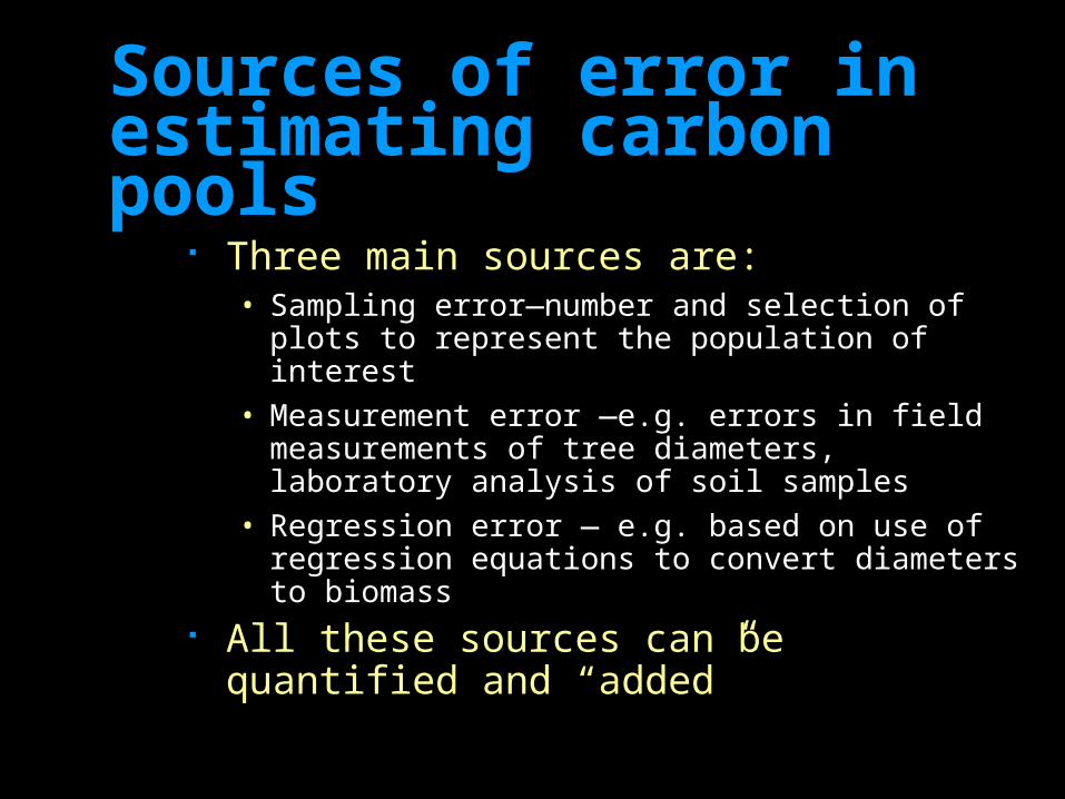
Sources of error in estimating carbon pools
Three main sources are:• Sampling error—number and selection of
plots to represent the population of interest• Measurement error —e.g. errors in field
measurements of tree diameters, laboratory analysis of soil samples
• Regression error — e.g. based on use of regression equations to convert diameters to biomass
All these sources can be quantified and “added”
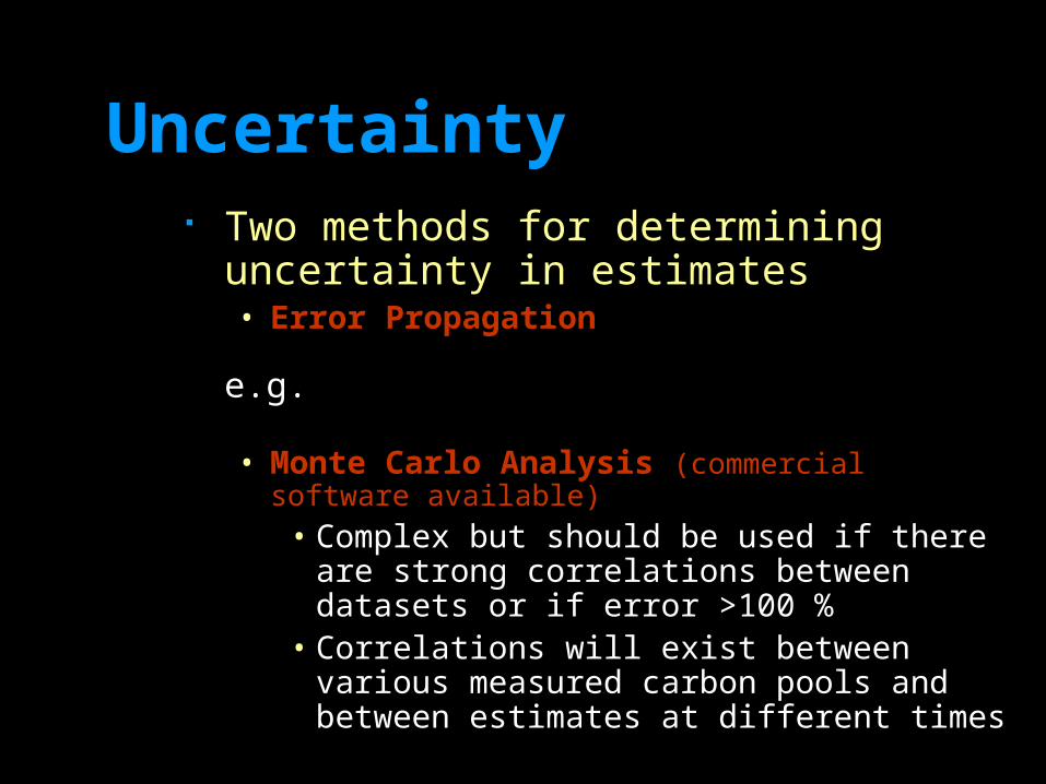
Uncertainty Two methods for determining
uncertainty in estimates• Error Propagation
• Monte Carlo Analysis (commercial software available)• Complex but should be used if there are
strong correlations between datasets or if error >100 %
• Correlations will exist between various measured carbon pools and between estimates at different times
22
21 %95%95%95 TimeTime CICICITotal e.g.
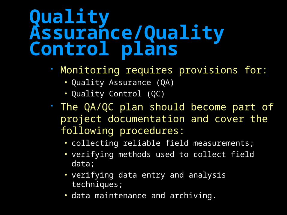
Quality Assurance/Quality Control plans
Monitoring requires provisions for:• Quality Assurance (QA) • Quality Control (QC)
The QA/QC plan should become part of project documentation and cover the following procedures:• collecting reliable field measurements; • verifying methods used to collect field data;• verifying data entry and analysis techniques; • data maintenance and archiving.
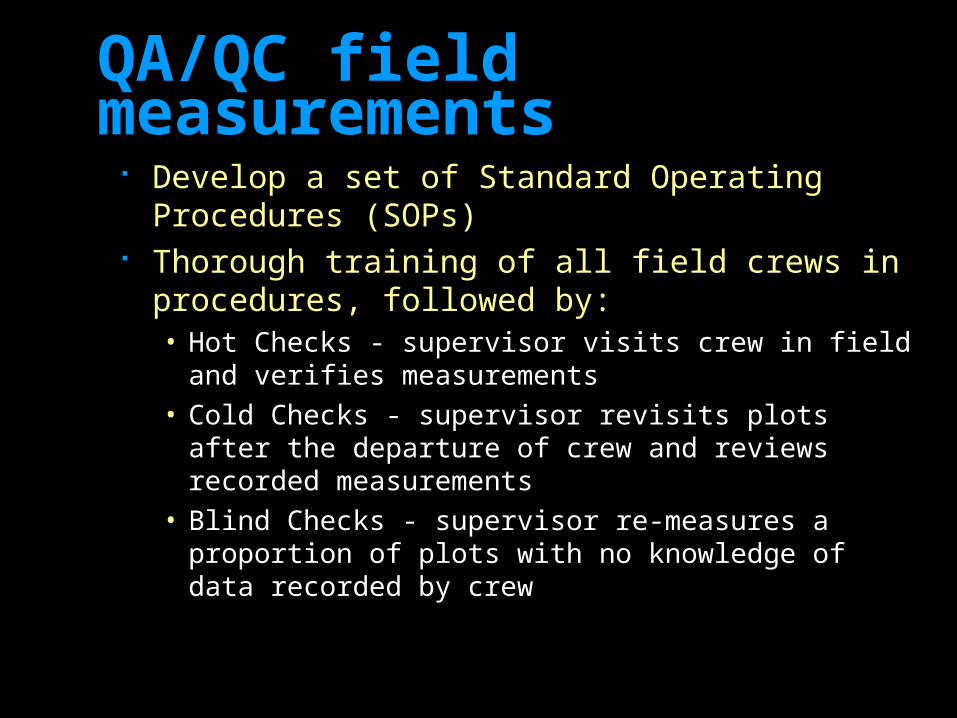
QA/QC field measurements Develop a set of Standard Operating
Procedures (SOPs) Thorough training of all field crews in
procedures, followed by:• Hot Checks - supervisor visits crew in field and
verifies measurements• Cold Checks - supervisor revisits plots after the
departure of crew and reviews recorded measurements
• Blind Checks - supervisor re-measures a proportion of plots with no knowledge of data recorded by crew
QA/QC for laboratory measurements, data entry, and archiving
Laboratory measurements• check equipment and measurement with
known quantity samples added blindly Data entry
• test of out of range values• recheck proportion for errors
Archiving• off-site storage of data

Acknowledgements
Team at Winrock International• Including Sandra Brown, Ken
MacDicken, David Shoch, Matt Delaney and John Kadyszewski
Funding agencies• Including TNC, USAID, USFS, UNDP
and World Bank