Embed Size (px)
Citation preview
Files and Storage: Intro
Jeff ChaseDuke University
Unix process view: data
Process
Thread
ProgramFiles
I/O channels(“file descriptors”)
stdinstdout
stderr
pipe
tty
socket
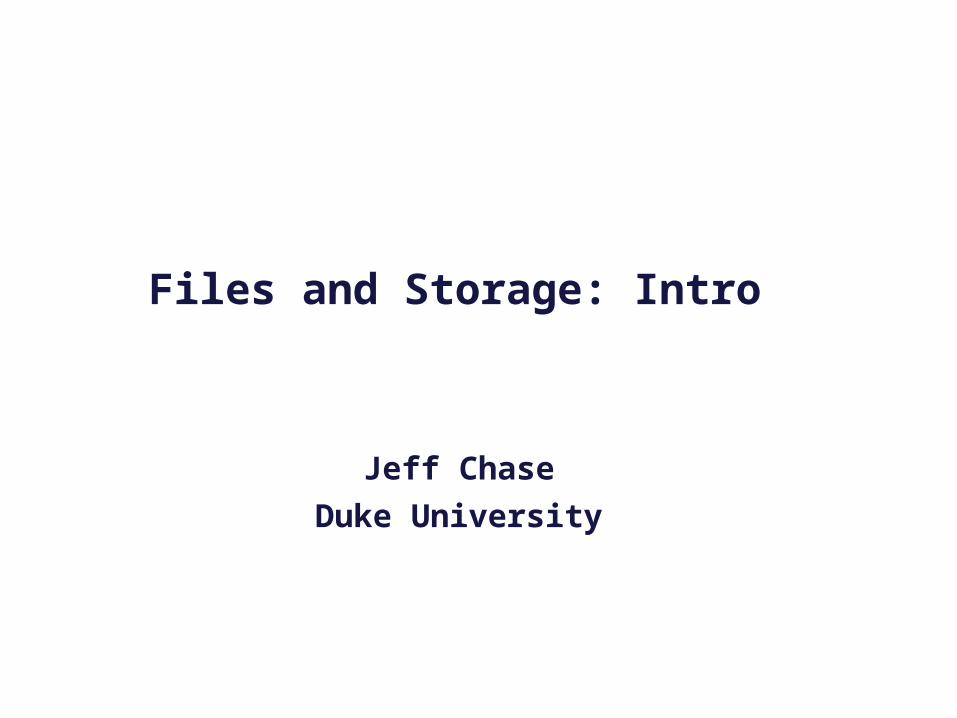
A process has multiple channels for data movement in and out of the process (I/O).
The parent process and parent program set up and control the channels for a child (until exec).
Files
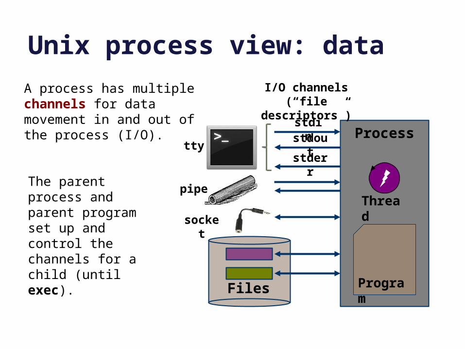
A file is a named, variable-length sequence of data bytes that is persistent: it exists across system restarts, and lives until it is removed.
Unix file syscallsfd = open(name, <options>);write(fd, “abcdefg”, 7);read(fd, buf, 7);lseek(fd, offset, SEEK_SET);close(fd);
creat(name, mode);fd = open(name, mode, O_CREAT);mkdir (name, mode);rmdir (name);unlink(name);
Files
An offset is a byte index in a file. By default, a process reads and writes files sequentially. Or it can seek to a particular offset.This is called a “logical seek” because it seeks to a particular location in the file, independent of where that data actually resides on storage (it could be anywhere).
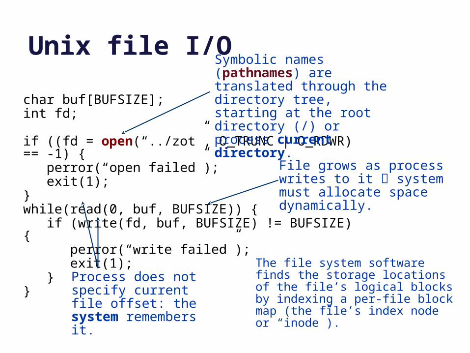
Unix file I/O
char buf[BUFSIZE];int fd;
if ((fd = open(“../zot”, O_TRUNC | O_RDWR) == -1) {perror(“open failed”);exit(1);
}while(read(0, buf, BUFSIZE)) {
if (write(fd, buf, BUFSIZE) != BUFSIZE) {perror(“write failed”);exit(1);
}}
Symbolic names (pathnames) are translated through the directory tree, starting at the root directory (/) or process current directory.
File grows as process writes to it system must allocate space dynamically.
Process does not specify current file offset: the system remembers it.
The file system software finds the storage locations of the file’s logical blocks by indexing a per-file block map (the file’s index node or “inode”).
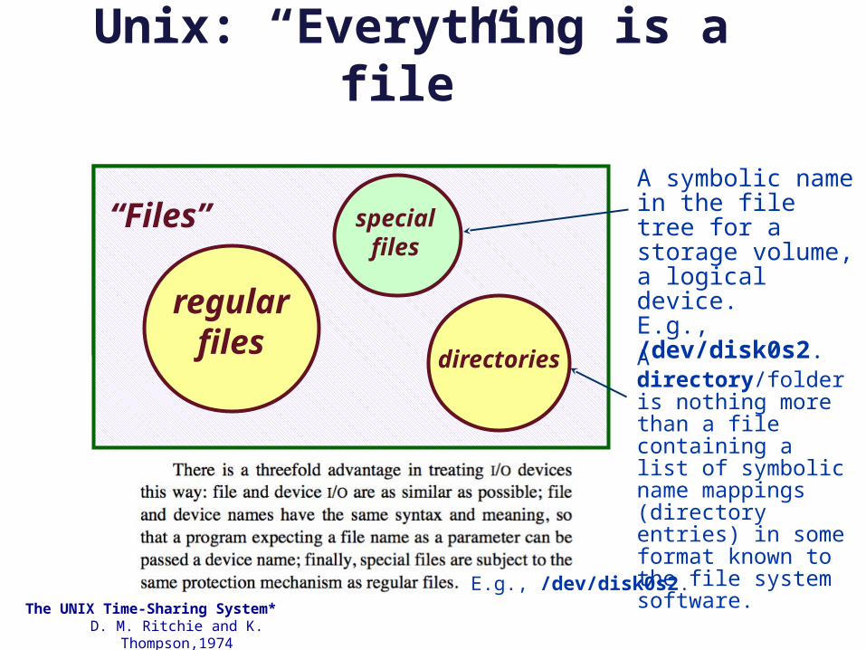
Unix: “Everything is a file”
Universal Set
A
B
regular files
“Files” special files
directories
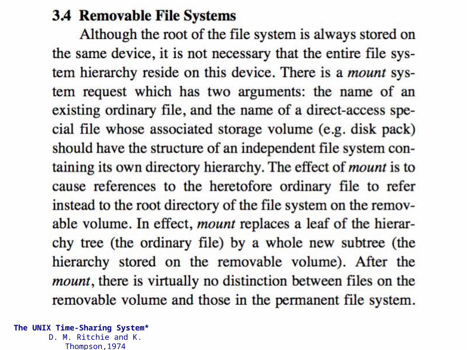
The UNIX Time-Sharing System* D. M. Ritchie and K. Thompson,1974
A symbolic name in the file tree for a storage volume, a logical device.E.g., /dev/disk0s2.
A directory/folder is nothing more than a file containing a list of symbolic name mappings (directory entries) in some format known to the file system software.
E.g., /dev/disk0s2.
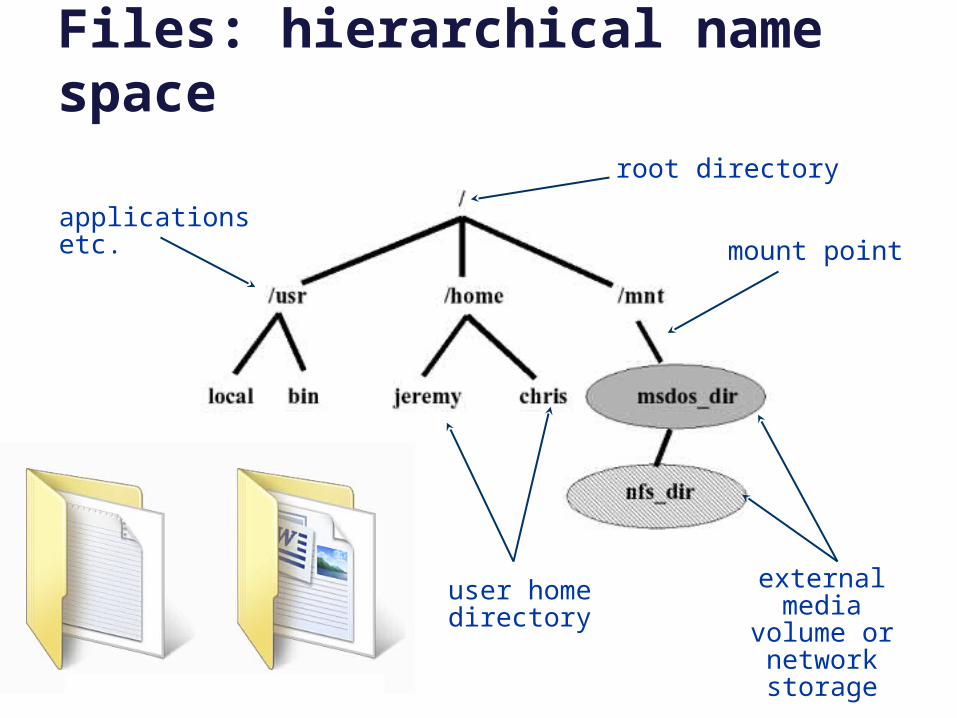
Files: hierarchical name spaceroot directory
mount point
user home directory
external media volume or network storage
applications etc.
/
tmp usretc
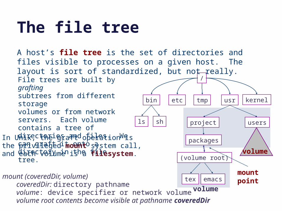
File trees are built by graftingsubtrees from different storagevolumes or from network servers. Each volume contains a tree of directories and files. We can graft it onto a directory in the file tree.
A host’s file tree is the set of directories and files visible to processes on a given host. The layout is sort of standardized, but not really.
bin kernel
ls sh project users
packages
(volume root)
tex emacs
In Unix, the graft operation isthe privileged mount system call,and each volume is a filesystem.
mount (coveredDir, volume)coveredDir: directory pathnamevolume: device specifier or network volumevolume root contents become visible at pathname coveredDir
The file tree
mount point
volume
volume
The UNIX Time-Sharing System* D. M. Ritchie and K. Thompson,1974
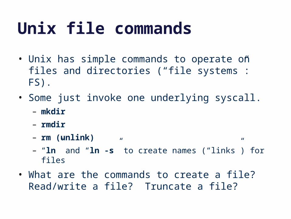
Unix file commands
• Unix has simple commands to operate on files and directories (“file systems”: FS).
• Some just invoke one underlying syscall.– mkdir
– rmdir
– rm (unlink)
– “ln” and “ln -s” to create names (“links”) for files
• What are the commands to create a file? Read/write a file? Truncate a file?
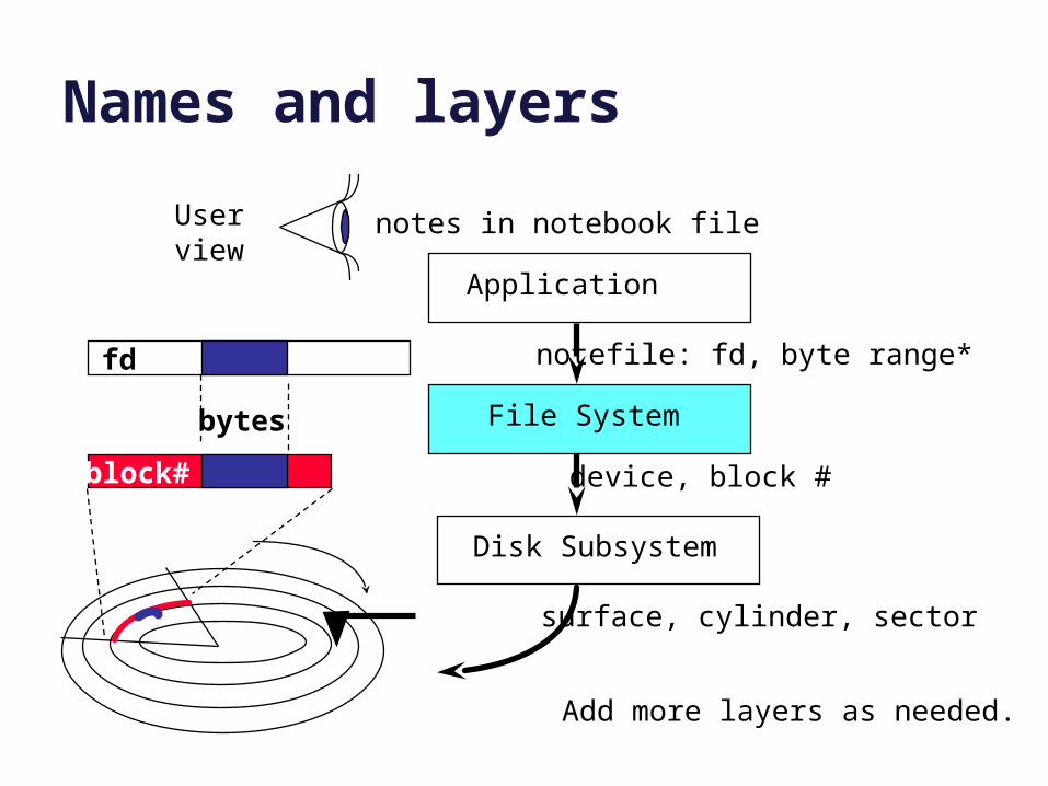
Names and layers
notes in notebook fileUserview
Application
File System
notefile: fd, byte range*
Disk Subsystem
device, block #
surface, cylinder, sector
bytes
fd
block#
Add more layers as needed.
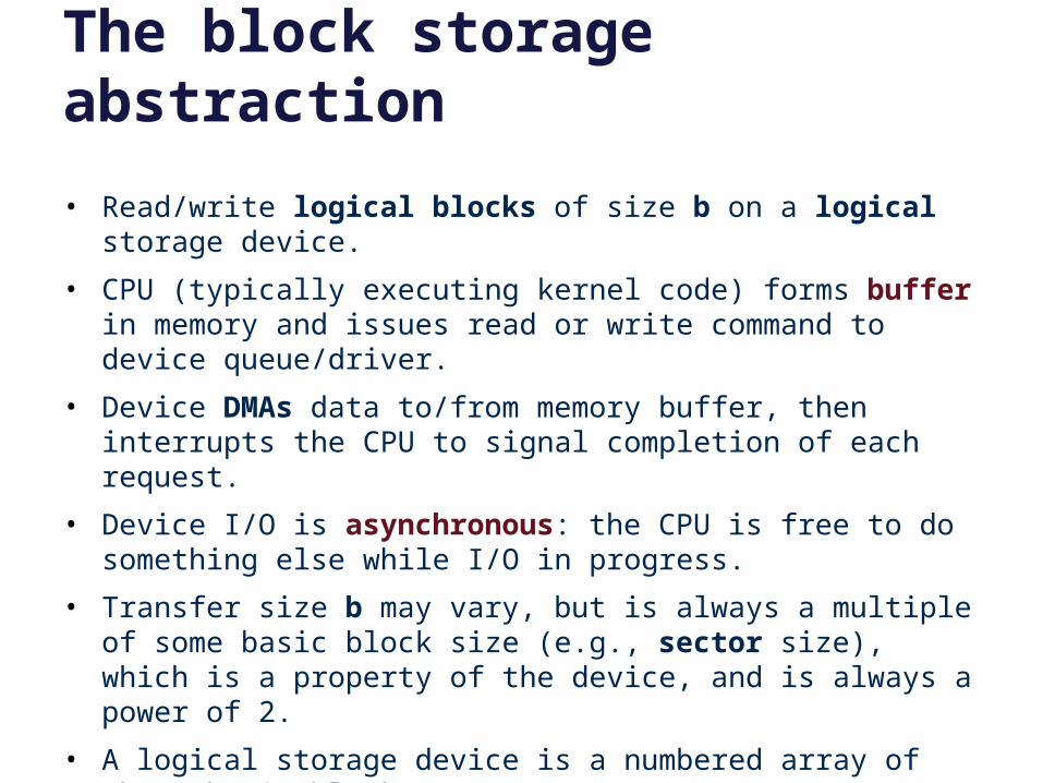
The block storage abstraction
• Read/write logical blocks of size b on a logical storage device.
• CPU (typically executing kernel code) forms buffer in memory and issues read or write command to device queue/driver.
• Device DMAs data to/from memory buffer, then interrupts the CPU to signal completion of each request.
• Device I/O is asynchronous: the CPU is free to do something else while I/O in progress.
• Transfer size b may vary, but is always a multiple of some basic block size (e.g., sector size), which is a property of the device, and is always a power of 2.
• A logical storage device is a numbered array of these basic blocks.
• Storage blocks containing data/metadata are cached in memory buffers while in active use: called buffer cache or block cache.
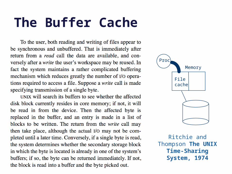
The Buffer Cache
Memory
Filecache
Proc
Ritchie and Thompson The UNIX Time-Sharing
System, 1974
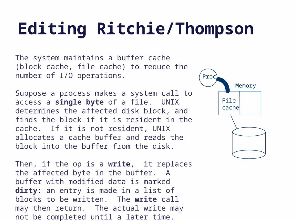
Editing Ritchie/Thompson
Memory
Filecache
Proc
The system maintains a buffer cache (block cache, file cache) to reduce the number of I/O operations.
Suppose a process makes a system call to access a single byte of a file. UNIX determines the affected disk block, and finds the block if it is resident in the cache. If it is not resident, UNIX allocates a cache buffer and reads the block into the buffer from the disk.
Then, if the op is a write, it replaces the affected byte in the buffer. A buffer with modified data is marked dirty: an entry is made in a list of blocks to be written. The write call may then return. The actual write may not be completed until a later time.
If the op is a read, it picks the requested byte out of the buffer and returns it, leaving the block in the cache.
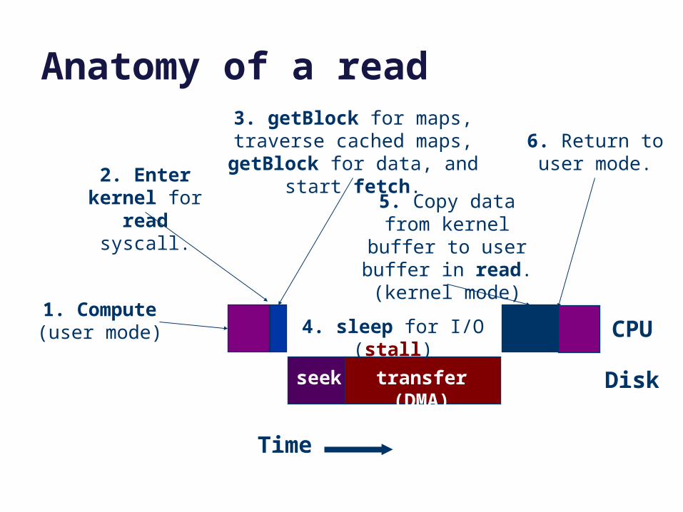
Anatomy of a read
1. Compute(user mode)
2. Enter kernel for read syscall.
3. getBlock for maps, traverse cached maps,
getBlock for data, and start fetch.
seek transfer (DMA)
4. sleep for I/O (stall)
5. Copy data from kernel buffer to user
buffer in read.(kernel mode)
CPU
Disk
6. Return to user mode.
Time
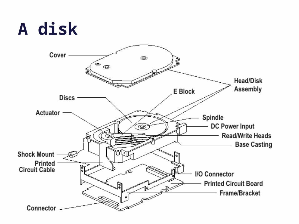
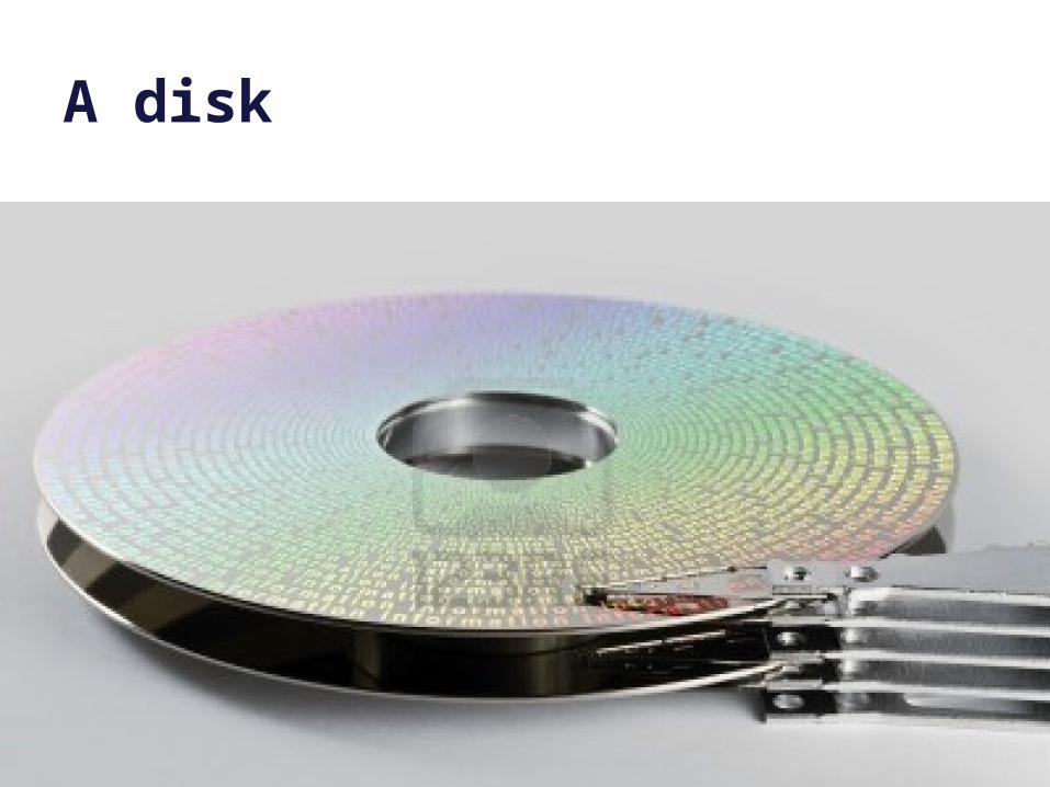
A disk
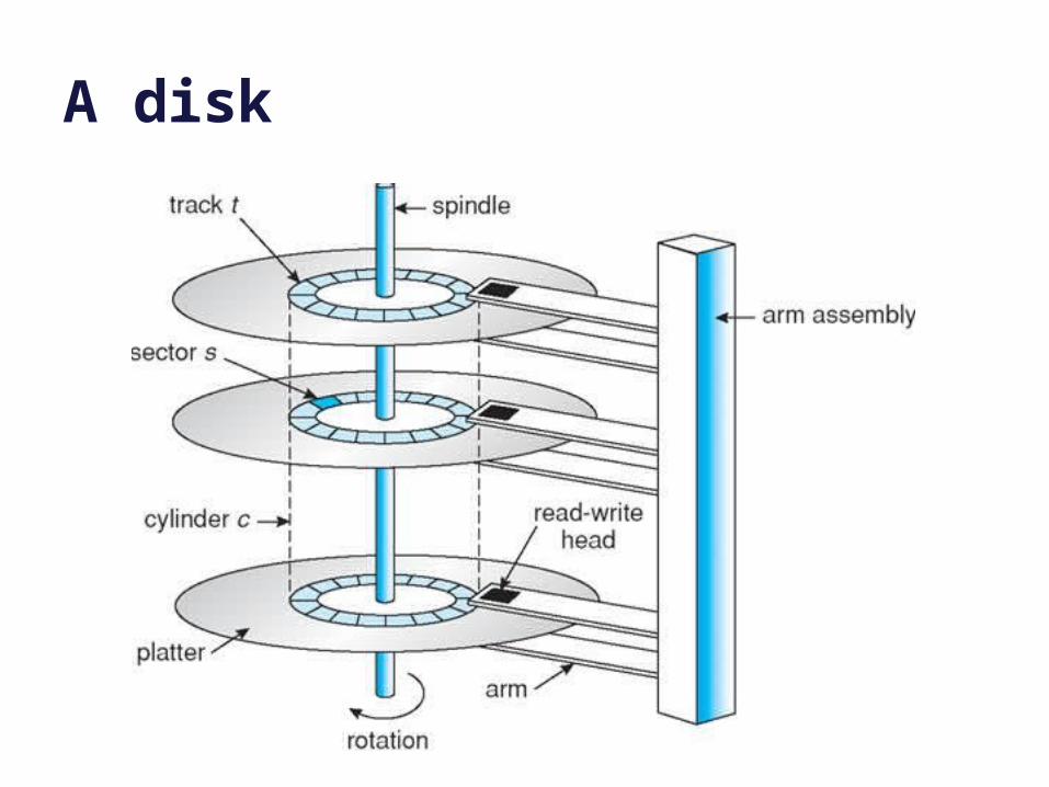
A disk
A disk
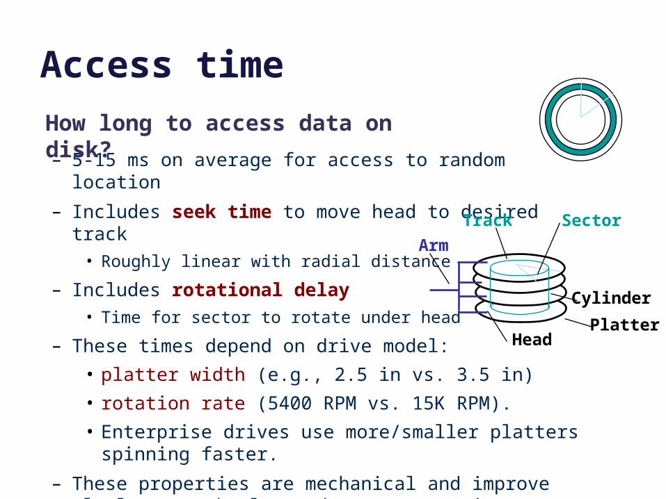
Access time
– 5-15 ms on average for access to random location
– Includes seek time to move head to desired track• Roughly linear with radial distance
– Includes rotational delay• Time for sector to rotate under head
– These times depend on drive model:
• platter width (e.g., 2.5 in vs. 3.5 in)
• rotation rate (5400 RPM vs. 15K RPM).
• Enterprise drives use more/smaller platters spinning faster.
– These properties are mechanical and improve slowly as technology advances over time.
SectorTrack
Cylinder
HeadPlatter
Arm
How long to access data on disk?
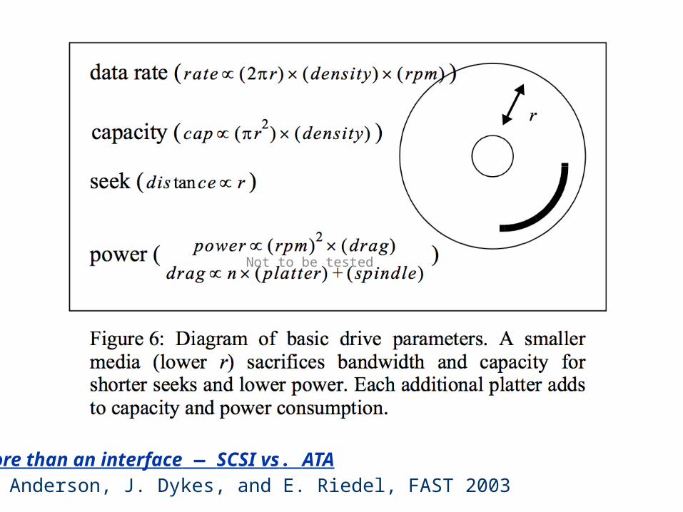
More than an interface — SCSI vs. ATAD. Anderson, J. Dykes, and E. Riedel, FAST 2003
Not to be tested
A few words about SSDs
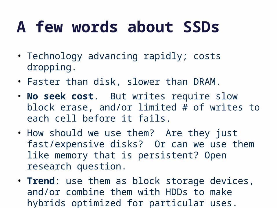
• Technology advancing rapidly; costs dropping.
• Faster than disk, slower than DRAM.
• No seek cost. But writes require slow block erase, and/or limited # of writes to each cell before it fails.
• How should we use them? Are they just fast/expensive disks? Or can we use them like memory that is persistent? Open research question.
• Trend: use them as block storage devices, and/or combine them with HDDs to make hybrids optimized for particular uses.– Examples everywhere you look.
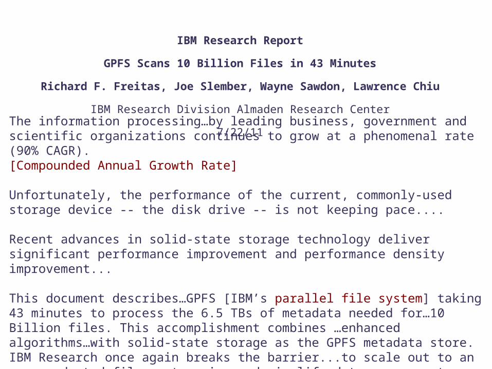
The information processing…by leading business, government and scientific organizations continues to grow at a phenomenal rate (90% CAGR).[Compounded Annual Growth Rate]
Unfortunately, the performance of the current, commonly-used storage device -- the disk drive -- is not keeping pace....
Recent advances in solid-state storage technology deliver significant performance improvement and performance density improvement...
This document describes…GPFS [IBM’s parallel file system] taking 43 minutes to process the 6.5 TBs of metadata needed for…10 Billion files. This accomplishment combines …enhanced algorithms…with solid-state storage as the GPFS metadata store. IBM Research once again breaks the barrier...to scale out to an unprecedented file system size…and simplify data management tasks, such as placement, aging, backup and replication..
IBM Research Report
GPFS Scans 10 Billion Files in 43 Minutes
Richard F. Freitas, Joe Slember, Wayne Sawdon, Lawrence Chiu
IBM Research Division Almaden Research Center
7/22/11
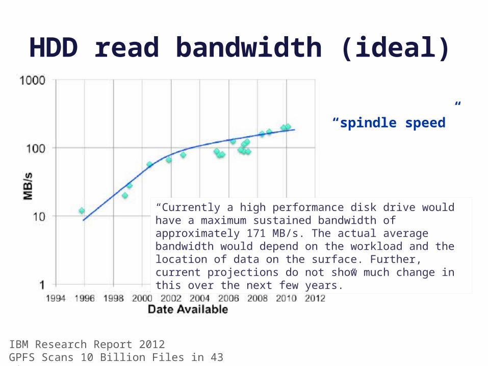
HDD read bandwidth (ideal)
“Currently a high performance disk drive would have a maximum sustained bandwidth of approximately 171 MB/s. The actual average bandwidth would depend on the workload and the location of data on the surface. Further, current projections do not show much change in this over the next few years.”
IBM Research Report 2012GPFS Scans 10 Billion Files in 43 Minutes
“spindle speed”
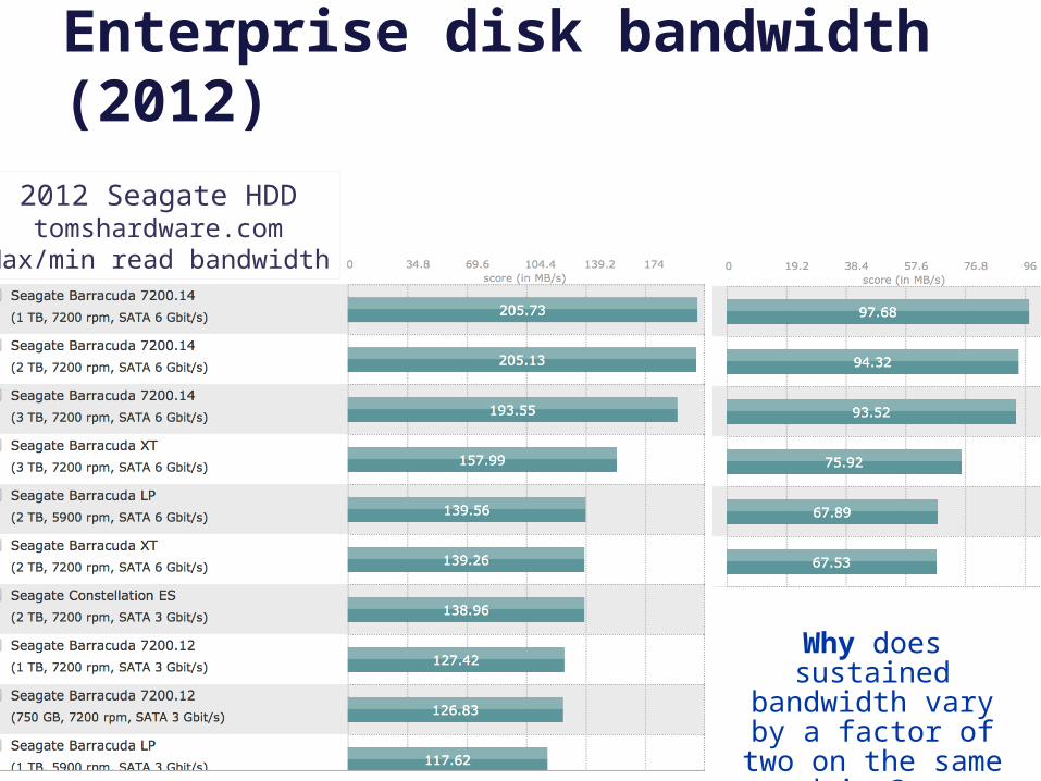
2012 Seagate HDDtomshardware.com
Max/min read bandwidth
Enterprise disk bandwidth (2012)
Why does sustained bandwidth vary by a factor of two on the
same drive?
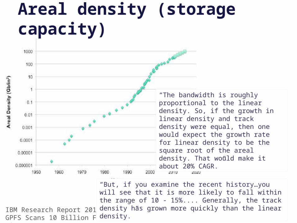
Areal density (storage capacity)
“The bandwidth is roughly proportional to the linear density. So, if the growth in linear density and track density were equal, then one would expect the growth rate for linear density to be the square root of the areal density. That would make it about 20% CAGR.”
IBM Research Report 2011GPFS Scans 10 Billion Files in 43 Minutes
“But, if you examine the recent history…you will see that it is more likely to fall within the range of 10 - 15%.... Generally, the track density has grown more quickly than the linear density.”
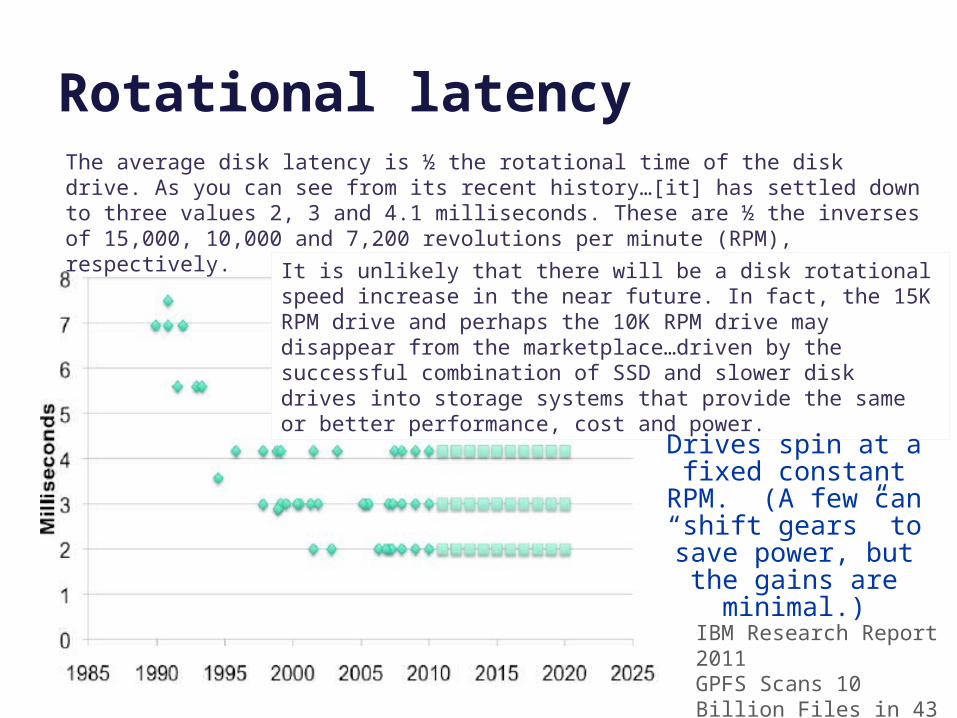
Rotational latencyThe average disk latency is ½ the rotational time of the disk drive. As you can see from its recent history…[it] has settled down to three values 2, 3 and 4.1 milliseconds. These are ½ the inverses of 15,000, 10,000 and 7,200 revolutions per minute (RPM), respectively.
It is unlikely that there will be a disk rotational speed increase in the near future. In fact, the 15K RPM drive and perhaps the 10K RPM drive may disappear from the marketplace…driven by the successful combination of SSD and slower disk drives into storage systems that provide the same or better performance, cost and power.
IBM Research Report 2011GPFS Scans 10 Billion Files in 43 Minutes
Drives spin at a fixed constant RPM. (A few
can “shift gears” to save power, but the gains are minimal.)
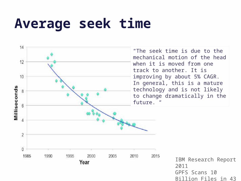
Average seek time
“The seek time is due to the mechanical motion of the head when it is moved from one track to another. It is improving by about 5% CAGR. In general, this is a mature technology and is not likely to change dramatically in the future. “
IBM Research Report 2011GPFS Scans 10 Billion Files in 43 Minutes
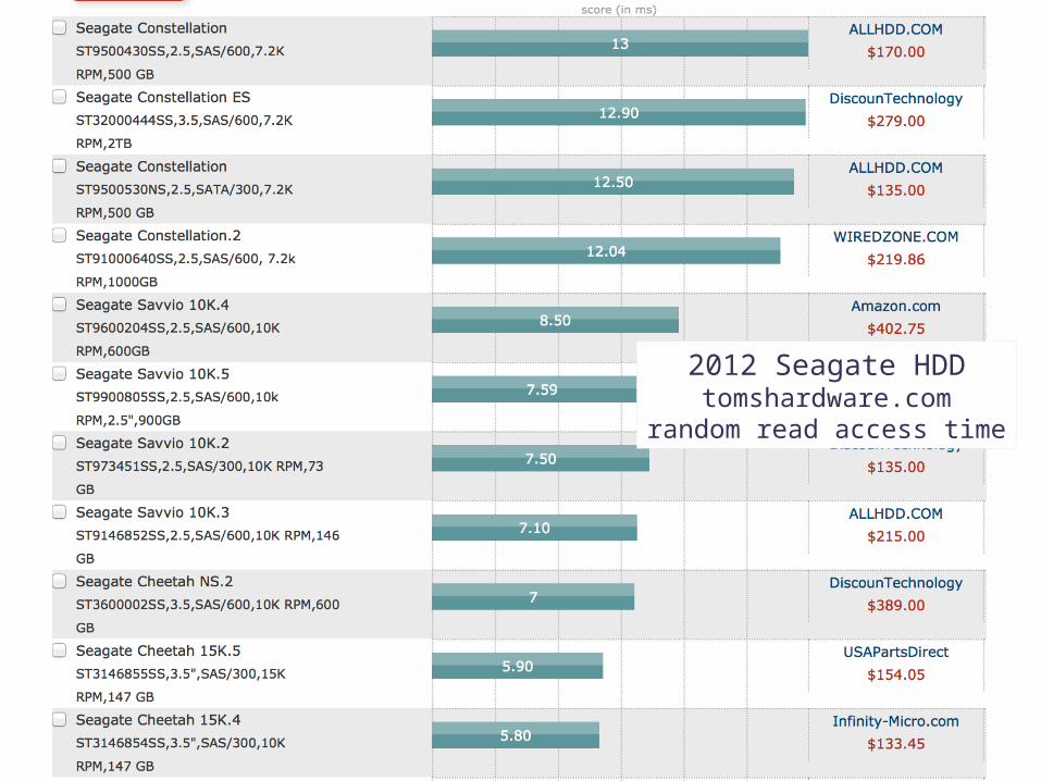
2012 Seagate HDDtomshardware.com
random read access time
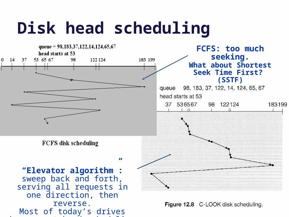
Disk head schedulingFCFS: too much seeking.
“Elevator algorithm”: sweep back and forth, serving all requests in
one direction, then reverse.Most of today’s drives have smart
head scheduling built in.
What about Shortest Seek Time First? (SSTF)
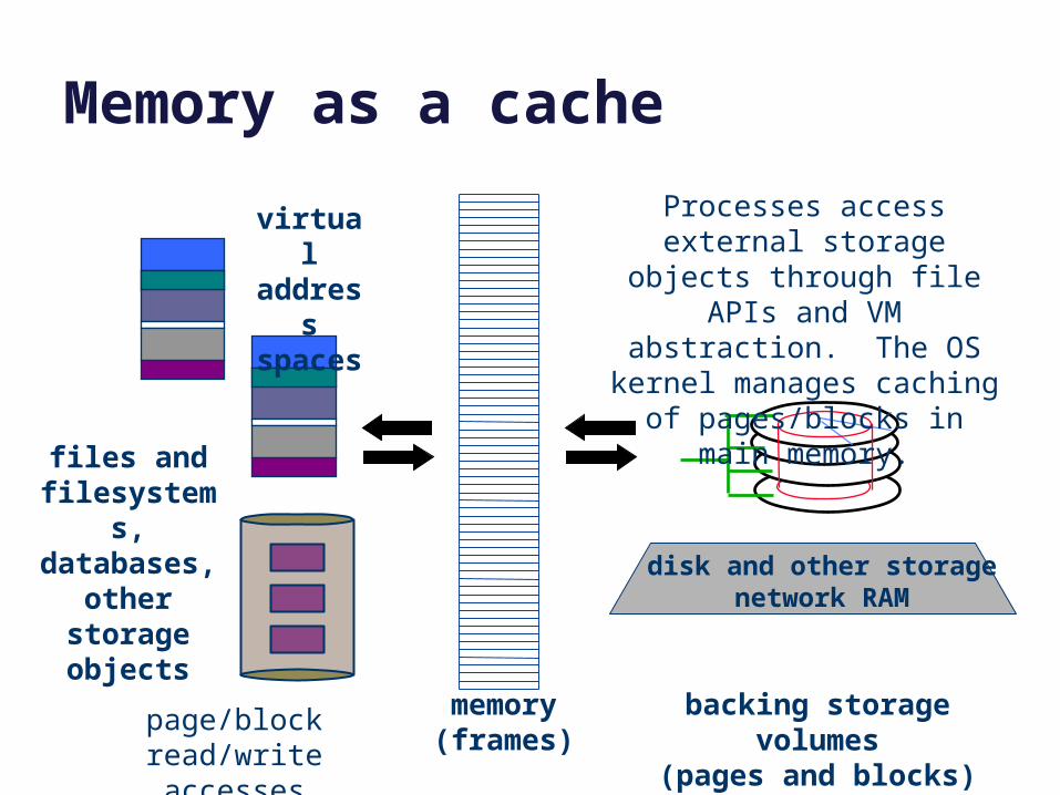
Memory as a cache
memory(frames)
data
data
virtual address spaces
files and filesystems,databases,
other storage objects
disk and other storagenetwork RAM
page/block read/write accesses
backing storage volumes(pages and blocks)
Processes access external storage objects through file
APIs and VM abstraction. The OS kernel manages caching
of pages/blocks in main memory.

registerscachesL1/L2
L3
main memory (RAM)
disk, other storage, network RAM
off-core
off-chip
off-module
small and fast
(ns)
big and slow(ms)
Memory/storage hierarchy
• In general, each layer is a cache over the layer below.
– inclusion property
• Technology trends rapid change
• The triangle is expanding vertically bigger gaps, more levels
Terms to knowcache index/directorycache line/entry, associativitycache hit/miss, hit ratiospatial locality of referencetemporal locality of referenceeviction / replacementwrite-through / writebackdirty/clean
File Systems and StoragePart the Second
Jeff ChaseDuke University
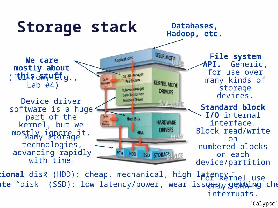
Storage stack
[Calypso]
File system API. Generic, for use
over many kinds of storage devices.
Standard block I/O internal interface.
Block read/write onnumbered blocks on each device/partition.For kernel use only: DMA + interrupts.
We care mostly about this stuff.
(for now, e.g., Lab #4)
Many storage technologies, advancing
rapidly with time.
Device driver software is a huge part of the kernel, but we mostly ignore it.
Rotational disk (HDD): cheap, mechanical, high latency.Solid-state “disk” (SSD): low latency/power, wear issues, getting cheaper.
Databases, Hadoop, etc.
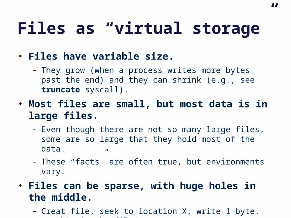
Files as “virtual storage”
• Files have variable size.– They grow (when a process writes more bytes past the end) and
they can shrink (e.g., see truncate syscall).
• Most files are small, but most data is in large files.– Even though there are not so many large files, some are so
large that they hold most of the data.
– These “facts” are often true, but environments vary.
• Files can be sparse, with huge holes in the middle.– Creat file, seek to location X, write 1 byte. How big is the file?
• Files come and go; some live long, some die young.
• How to implement diverse files on shared storage?
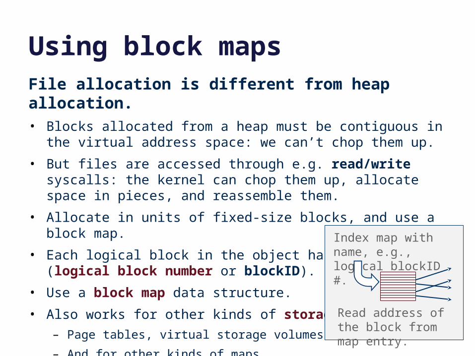
Using block mapsFile allocation is different from heap allocation.• Blocks allocated from a heap must be contiguous in the virtual
address space: we can’t chop them up.
• But files are accessed through e.g. read/write syscalls: the kernel can chop them up, allocate space in pieces, and reassemble them.
• Allocate in units of fixed-size blocks, and use a block map.
• Each logical block in the object has an address (logical block number or blockID).
• Use a block map data structure.
• Also works for other kinds of storage objects
– Page tables, virtual storage volumes
– And for other kinds of maps…
– Implement in-memory cache with a hash table
Index map with name, e.g., logical blockID #.
Read address of the block from map entry.
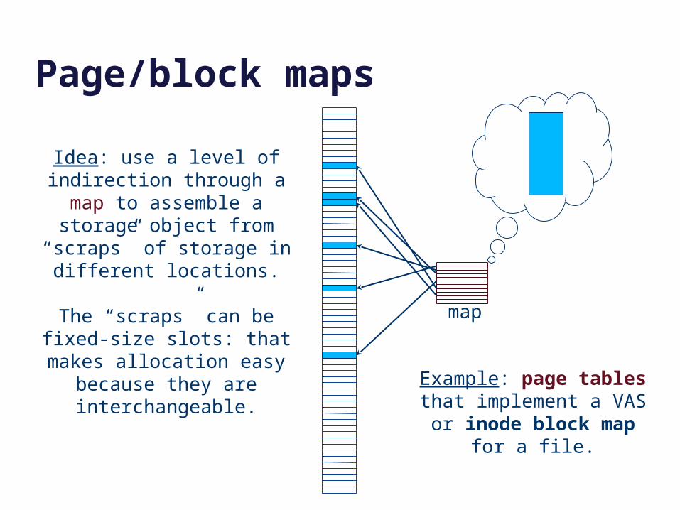
Page/block maps
map
Idea: use a level of indirection through a map to assemble a
storage object from “scraps” of storage in different locations.
The “scraps” can be fixed-size slots: that makes allocation
easy because they are interchangeable.
Example: page tables that implement a VAS or inode
block map for a file.
http://web.mit.edu/6.033/2001/wwwdocs/handouts/naming_review.html
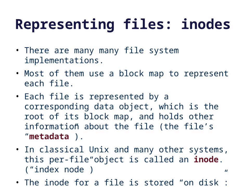
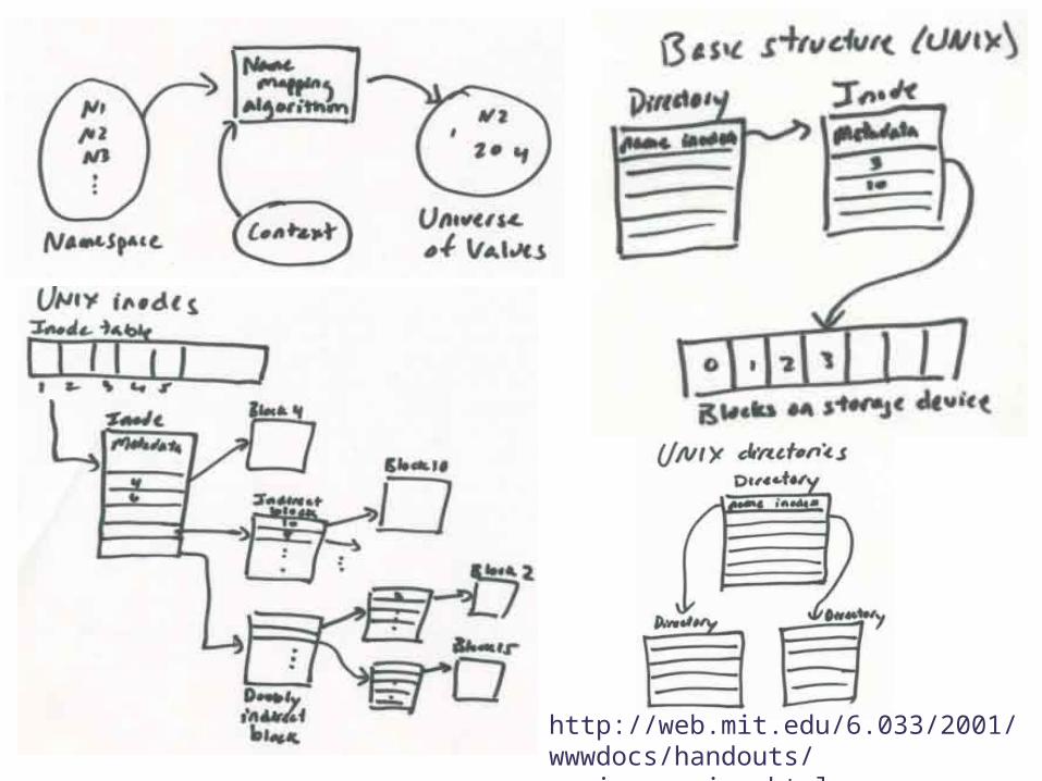
Representing files: inodes
• There are many many file system implementations.
• Most of them use a block map to represent each file.
• Each file is represented by a corresponding data object, which is the root of its block map, and holds other information about the file (the file’s “metadata”).
• In classical Unix and many other systems, this per-file object is called an inode. (“index node”)
• The inode for a file is stored “on disk”: the OS/FS reads it in and keeps it in memory while the file is in active use.
• When a file is modified, the OS/FS writes any changes to its inode/maps back to the disk.
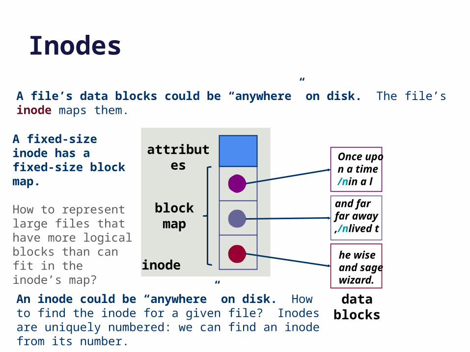
Inodes
inode
An inode could be “anywhere” on disk. How to find the inode for a given file? Inodes are uniquely numbered: we can find an inode from its number.
A fixed-size inode has a fixed-size block map.
How to represent large files that have more logical blocks than can fit in the inode’s map?
block map
Once upon a time/nin a l
and far far away,/nlived t
he wise and sagewizard.
attributes
data blocks
A file’s data blocks could be “anywhere” on disk. The file’s inode maps them.
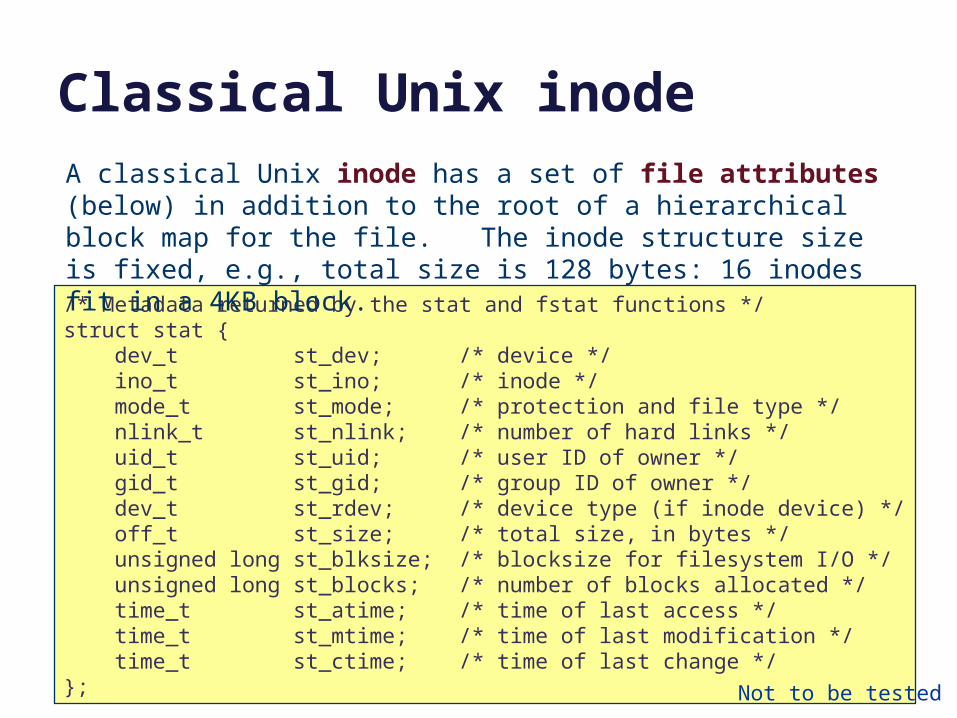
/* Metadata returned by the stat and fstat functions */struct stat { dev_t st_dev; /* device */ ino_t st_ino; /* inode */ mode_t st_mode; /* protection and file type */ nlink_t st_nlink; /* number of hard links */ uid_t st_uid; /* user ID of owner */ gid_t st_gid; /* group ID of owner */ dev_t st_rdev; /* device type (if inode device) */ off_t st_size; /* total size, in bytes */ unsigned long st_blksize; /* blocksize for filesystem I/O */ unsigned long st_blocks; /* number of blocks allocated */ time_t st_atime; /* time of last access */ time_t st_mtime; /* time of last modification */ time_t st_ctime; /* time of last change */}; Not to be tested
Classical Unix inodeA classical Unix inode has a set of file attributes (below) in addition to the root of a hierarchical block map for the file. The inode structure size is fixed, e.g., total size is 128 bytes: 16 inodes fit in a 4KB block.
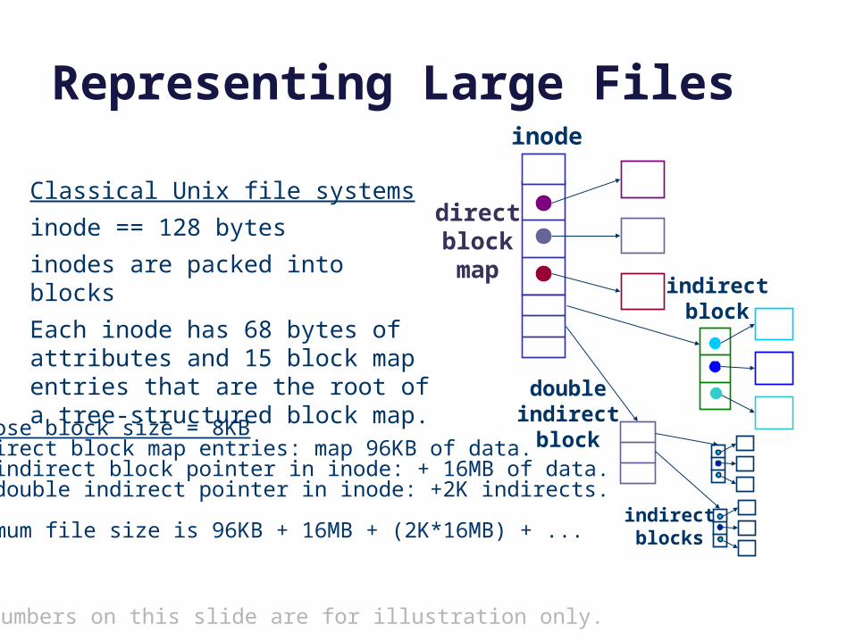
Representing Large Filesinode
indirectblock
doubleindirectblock
Suppose block size = 8KB12 direct block map entries: map 96KB of data.One indirect block pointer in inode: + 16MB of data.One double indirect pointer in inode: +2K indirects.
Maximum file size is 96KB + 16MB + (2K*16MB) + ...
Classical Unix file systems
inode == 128 bytes
inodes are packed into blocks
Each inode has 68 bytes of attributes and 15 block map entries that are the root of a tree-structured block map.
directblockmap
indirectblocks
The numbers on this slide are for illustration only.
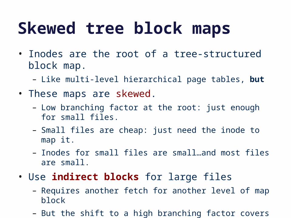
Skewed tree block maps
• Inodes are the root of a tree-structured block map.– Like multi-level hierarchical page tables, but
• These maps are skewed.– Low branching factor at the root: just enough for small files.
– Small files are cheap: just need the inode to map it.
– Inodes for small files are small…and most files are small.
• Use indirect blocks for large files– Requires another fetch for another level of map block
– But the shift to a high branching factor covers most large files.
• Double indirect blocks allow very large files.
• Other advantages to trees?
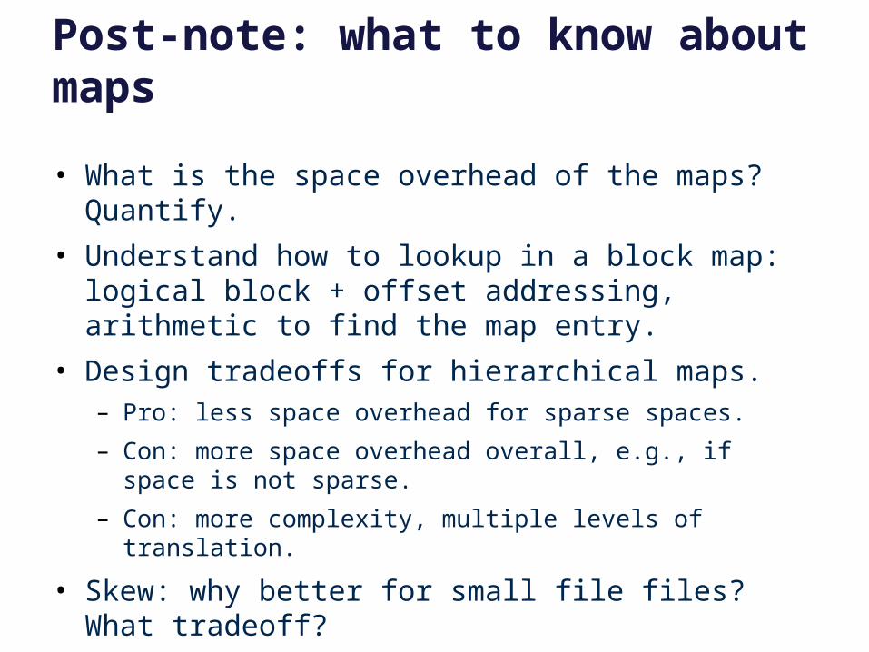
Post-note: what to know about maps
• What is the space overhead of the maps? Quantify.
• Understand how to lookup in a block map: logical block + offset addressing, arithmetic to find the map entry.
• Design tradeoffs for hierarchical maps.– Pro: less space overhead for sparse spaces.
– Con: more space overhead overall, e.g., if space is not sparse.
– Con: more complexity, multiple levels of translation.
• Skew: why better for small file files? What tradeoff?– No need to memorize the various parameters for inode maps: concept only.
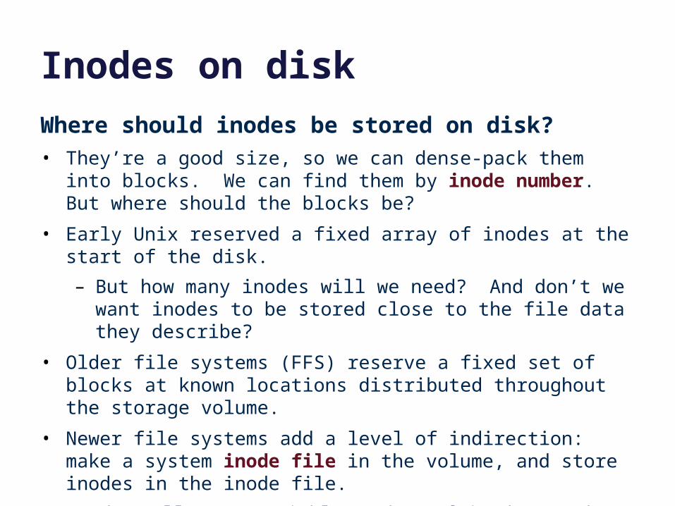
Inodes on disk
Where should inodes be stored on disk?• They’re a good size, so we can dense-pack them into blocks. We
can find them by inode number. But where should the blocks be?
• Early Unix reserved a fixed array of inodes at the start of the disk.
– But how many inodes will we need? And don’t we want inodes to be stored close to the file data they describe?
• Older file systems (FFS) reserve a fixed set of blocks at known locations distributed throughout the storage volume.
• Newer file systems add a level of indirection: make a system inode file in the volume, and store inodes in the inode file.
– That allows a variable number of inodes, and we can move them to different locations as they’re modified.
– Originated with Berkeley’s Log Structured File System (LFS) and NetApp’s Write Anywhere File Layout (WAFL).
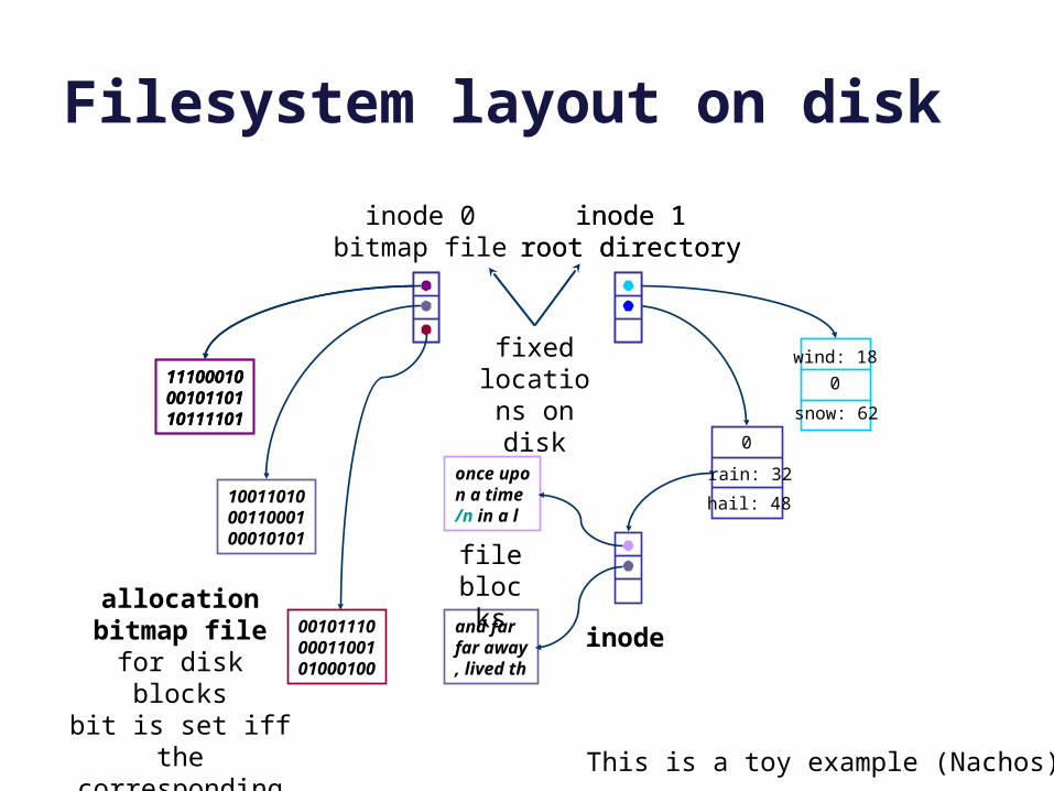
Filesystem layout on disk
111000100010110110111101
inode 0bitmap file
0
rain: 32
hail: 48
once upon a time/n in a l
and far far away, lived th
inode 1root directory
inode
file blocks
111000100010110110111101
100110100011000100010101
001011100001100101000100
allocationbitmap file
for disk blocksbit is set iff the
corresponding block is in use
0
wind: 18
snow: 62
inode 1root directory
fixed locations on disk
This is a toy example (Nachos).
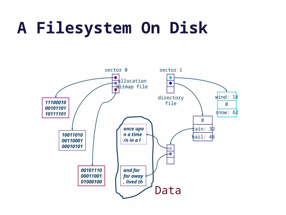
A Filesystem On Disk
111000100010110110111101
100110100011000100010101
001011100001100101000100
sector 0
allocationbitmap file
0
rain: 32
hail: 48
0
wind: 18
snow: 62
once upon a time/n in a l
and far far away, lived th
sector 1
directoryfile
Data
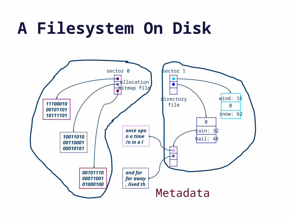
A Filesystem On Disk
111000100010110110111101
100110100011000100010101
001011100001100101000100
sector 0
allocationbitmap file
0
rain: 32
hail: 48
0
wind: 18
snow: 62
once upon a time/n in a l
and far far away, lived th
sector 1
directoryfile
Metadata
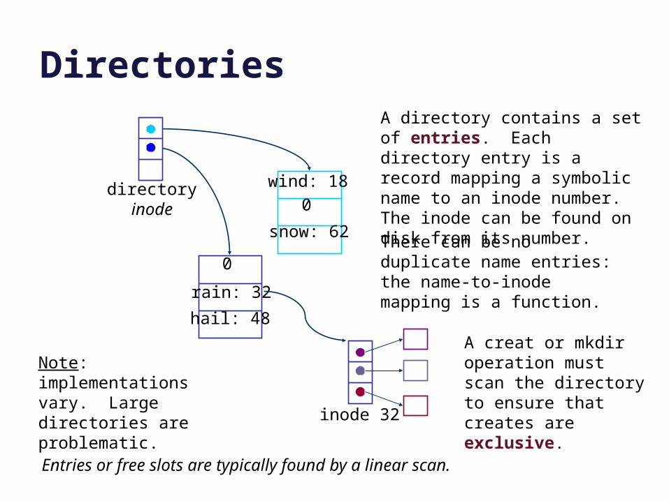
Directories
0
rain: 32
hail: 48
0
wind: 18
snow: 62
directoryinode
inode 32
Entries or free slots are typically found by a linear scan.
Note: implementations vary. Large directories are problematic.
A creat or mkdir operation must scan the directory to ensure that creates are exclusive.
There can be no duplicate name entries: the name-to-inode mapping is a function.
A directory contains a set of entries. Each directory entry is a record mapping a symbolic name to an inode number. The inode can be found on disk from its number.
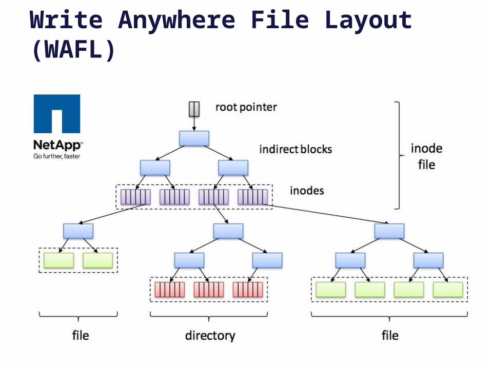
Write Anywhere File Layout (WAFL)
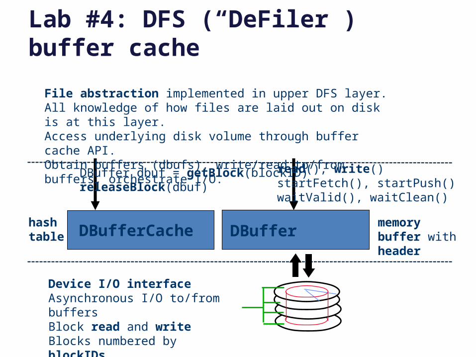
DBufferCache DBuffer
read(), write()startFetch(), startPush()waitValid(), waitClean()
DBuffer dbuf = getBlock(blockID)releaseBlock(dbuf)
Lab #4: DFS (“DeFiler”) buffer cache
Device I/O interfaceAsynchronous I/O to/from buffersBlock read and writeBlocks numbered by blockIDs
File abstraction implemented in upper DFS layer.All knowledge of how files are laid out on disk is at this layer.Access underlying disk volume through buffer cache API.Obtain buffers (dbufs), write/read to/from buffers, orchestrate I/O.
hash table
memory buffer with header
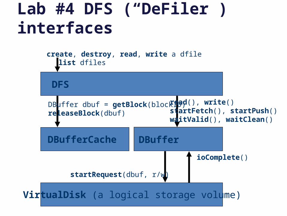
DFS
DBufferCache DBuffer
VirtualDisk (a logical storage volume)
startRequest(dbuf, r/w)
ioComplete()
read(), write()startFetch(), startPush()waitValid(), waitClean()
DBuffer dbuf = getBlock(blockID)releaseBlock(dbuf)
create, destroy, read, write a dfilelist dfiles
Lab #4 DFS (“DeFiler”) interfaces
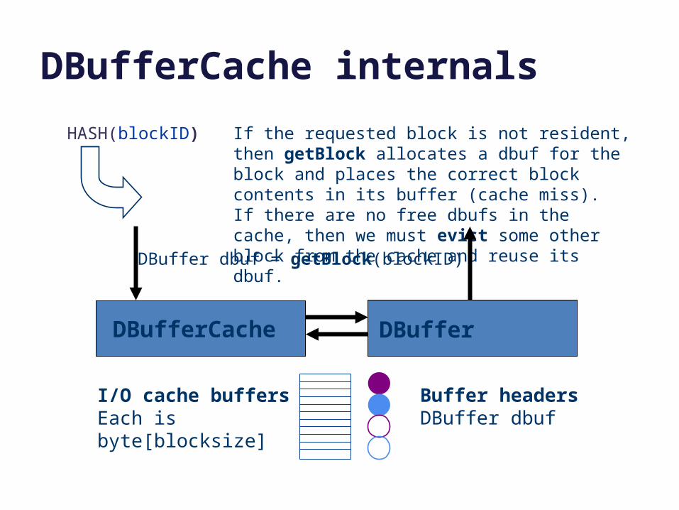
DBufferCache internals
DBufferCache DBuffer
I/O cache buffersEach is byte[blocksize]
Buffer headersDBuffer dbuf
HASH(blockID) If the requested block is not resident, then getBlock allocates a dbuf for the block and places the correct block contents in its buffer (cache miss). If there are no free dbufs in the cache, then we must evict some other block from the cache and reuse its dbuf.
DBuffer dbuf = getBlock(blockID)
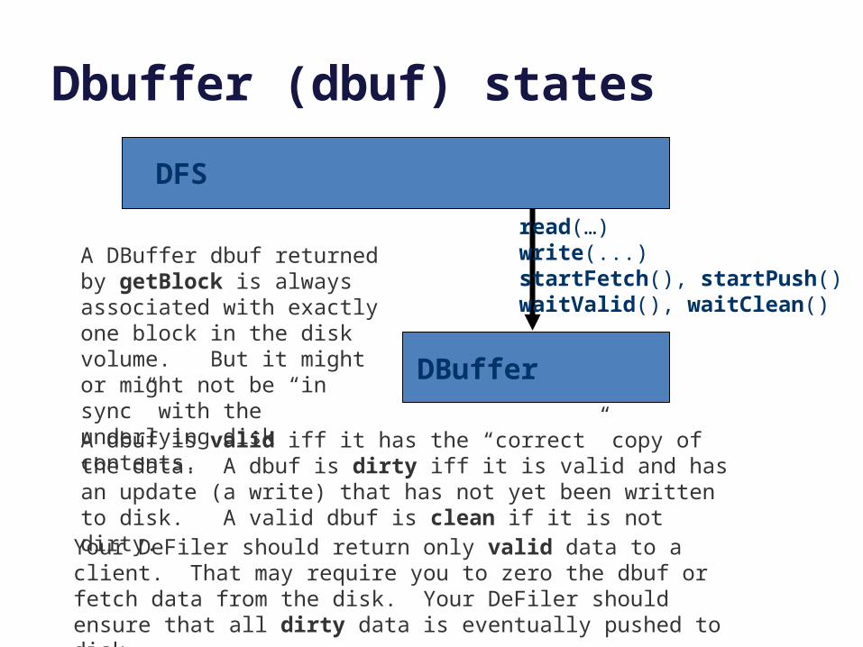
Dbuffer (dbuf) states
A DBuffer dbuf returned by getBlock is always associated with exactly one block in the disk volume. But it might or might not be “in sync” with the underlying disk contents.
DBuffer
read(…)write(...)startFetch(), startPush()waitValid(), waitClean()
DFS
A dbuf is valid iff it has the “correct” copy of the data. A dbuf is dirty iff it is valid and has an update (a write) that has not yet been written to disk. A valid dbuf is clean if it is not dirty.
Your DeFiler should return only valid data to a client. That may require you to zero the dbuf or fetch data from the disk. Your DeFiler should ensure that all dirty data is eventually pushed to disk.
DBuffer
startFetch(), startPush()waitValid(), waitClean()
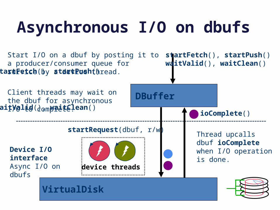
Asynchronous I/O on dbufs
startRequest(dbuf, r/w)
ioComplete()
VirtualDisk
device threads
Device I/O interfaceAsync I/O on dbufs
Start I/O on a dbuf by posting it to a producer/consumer queue for service by a device thread.
Thread upcalls dbuf ioComplete when I/O operation is done.
Client threads may wait on the dbuf for asynchronous I/O to complete.
startFetch(), startPush()
waitValid(), waitClean()
read(), write()startFetch(), startPush()waitValid(), waitClean()
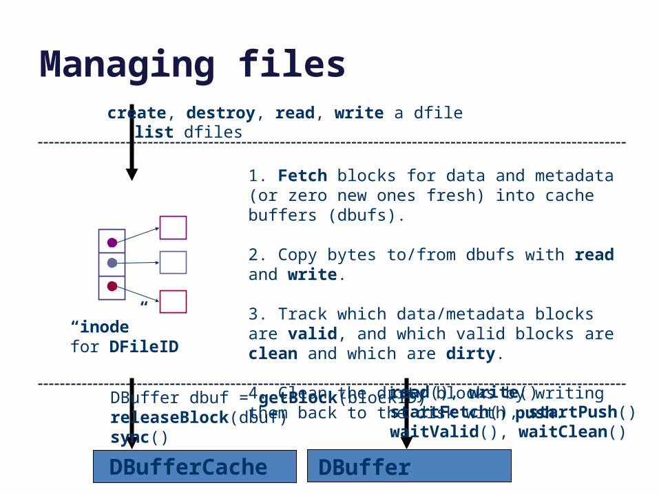
DBuffer dbuf = getBlock(blockID)releaseBlock(dbuf)sync()
create, destroy, read, write a dfilelist dfiles
Managing files
DBufferCache DBuffer
“inode”for DFileID
1. Fetch blocks for data and metadata (or zero new ones fresh) into cache buffers (dbufs).
2. Copy bytes to/from dbufs with read and write.
3. Track which data/metadata blocks are valid, and which valid blocks are clean and which are dirty.
4. Clean the dirty blocks by writing them back to the disk with push.
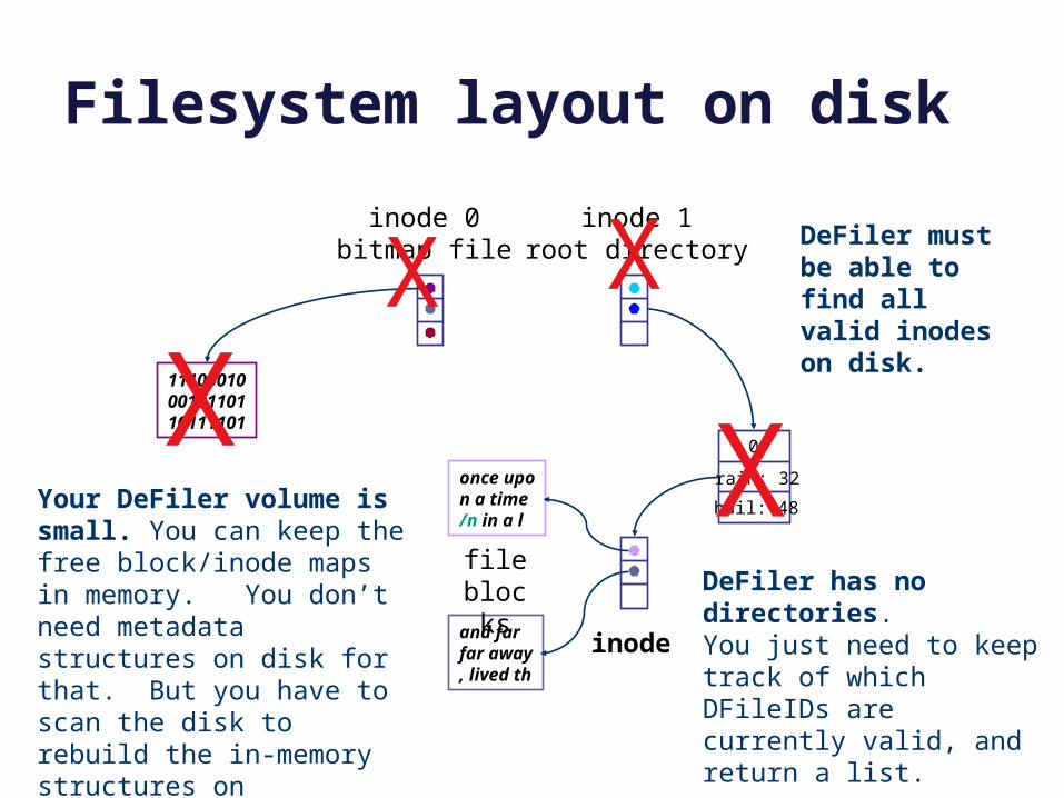
Filesystem layout on disk
111000100010110110111101
inode 0bitmap file
0
rain: 32
hail: 48
once upon a time/n in a l
and far far away, lived th
inode 1root directory
inode
file blocks
Your DeFiler volume is small. You can keep the free block/inode maps in memory. You don’t need metadata structures on disk for that. But you have to scan the disk to rebuild the in-memory structures on initialization.
X X
XX
DeFiler has no directories.You just need to keep track of which DFileIDs are currently valid, and return a list.
DeFiler must be able to find all valid inodes on disk.
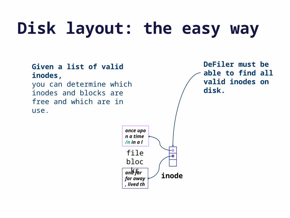
Disk layout: the easy way
once upon a time/n in a l
and far far away, lived th
inode
file blocks
Given a list of valid inodes,you can determine which inodes and blocks are free and which are in use.
DeFiler must be able to find all valid inodes on disk.
Unix file naming: hard links0
rain: 32
hail: 48
0
wind: 18
sleet: 48
inode 48
inode link count = 2
directory A directory B
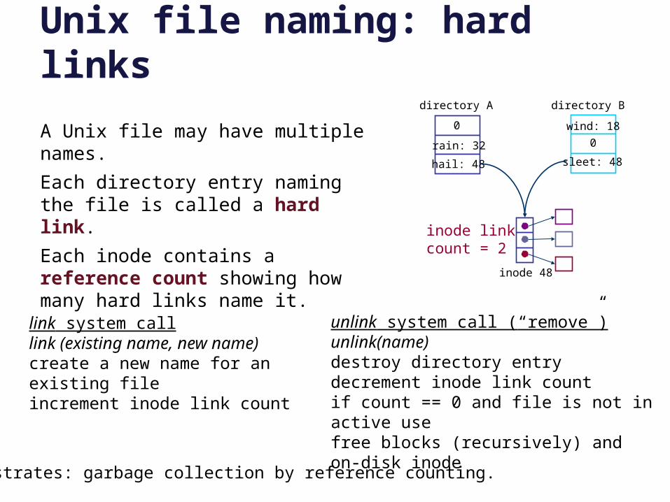
A Unix file may have multiple names.
Each directory entry naming the file is called a hard link.
Each inode contains a reference count showing how many hard links name it.
Illustrates: garbage collection by reference counting.
link system calllink (existing name, new name)create a new name for an existing fileincrement inode link count
unlink system call (“remove”)unlink(name)destroy directory entrydecrement inode link countif count == 0 and file is not in active usefree blocks (recursively) and on-disk inode
Unix file naming: soft links
0
rain: 32
hail: 48
inode 48
inode link count = 1
directory A
0
wind: 18
sleet: 67
directory B
../A/hail/0
inode 67
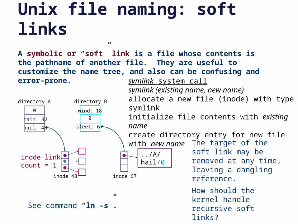
The target of the soft link may be removed at any time, leaving a dangling reference.
How should the kernel handle recursive soft links?
symlink system callsymlink (existing name, new name)allocate a new file (inode) with type symlinkinitialize file contents with existing namecreate directory entry for new file with new name
A symbolic or “soft” link is a file whose contents is the pathname of another file. They are useful to customize the name tree, and also can be confusing and error-prone.
See command “ln –s”.
Unix file naming: links
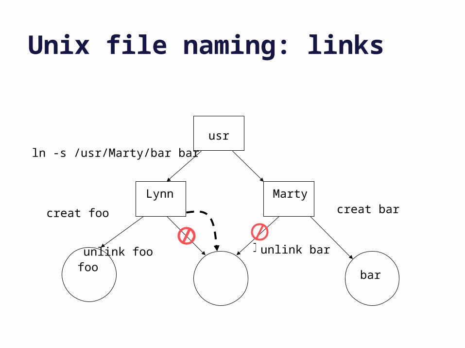
usr
Lynn Marty
ln /usr/Lynn/foo barunlink foofoo
creat foo
ln -s /usr/Marty/bar bar
unlink bar
creat bar
bar
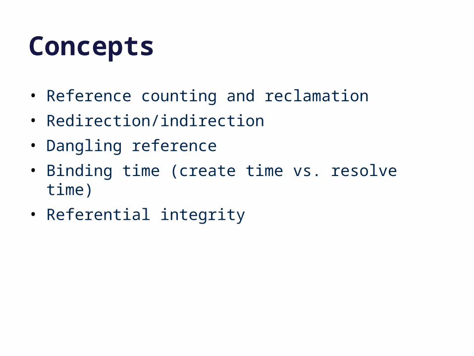
Concepts
• Reference counting and reclamation
• Redirection/indirection
• Dangling reference
• Binding time (create time vs. resolve time)
• Referential integrity
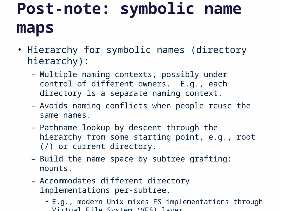
Post-note: symbolic name maps• Hierarchy for symbolic names (directory hierarchy):
– Multiple naming contexts, possibly under control of different owners. E.g., each directory is a separate naming context.
– Avoids naming conflicts when people reuse the same names.
– Pathname lookup by descent through the hierarchy from some starting point, e.g., root (/) or current directory.
– Build the name space by subtree grafting: mounts.
– Accommodates different directory implementations per-subtree.• E.g., modern Unix mixes FS implementations through Virtual File
System (VFS) layer.
– Scales to very large name spaces.
• Note: Domain Name Service (DNS) is the same!– www.cs.duke.edu “==“ /edu/duke/cs/www
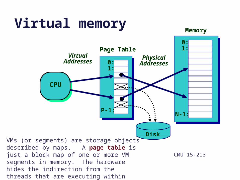
Virtual memory
CPU
0:1:
N-1:
Memory
0:1:
P-1:
Page Table
Disk
VirtualAddresses
PhysicalAddresses
CMU 15-213
VMs (or segments) are storage objects described by maps. A page table is just a block map of one or more VM segments in memory. The hardware hides the indirection from the threads that are executing within that VM.
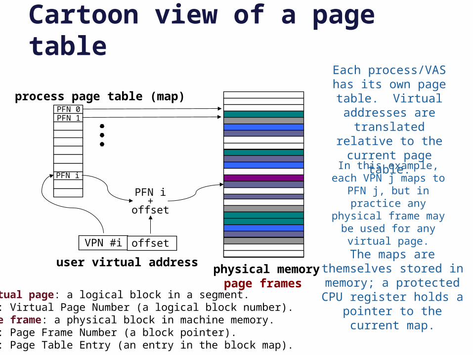
Cartoon view of a page table
PFN 0PFN 1
PFN i
VPN #i offset
user virtual address
PFN i+
offset
process page table (map)
physical memorypage frames
In this example, each VPN j maps to PFN j, but in practice any physical frame may be used for
any virtual page.
Each process/VAS has its own page table.
Virtual addresses are translated relative to
the current page table.
The maps are themselves stored in memory; a
protected CPU register holds a pointer to the
current map.
Virtual page: a logical block in a segment.VPN: Virtual Page Number (a logical block number).Page frame: a physical block in machine memory.PFN: Page Frame Number (a block pointer).PTE: Page Table Entry (an entry in the block map).
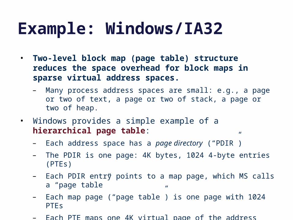
Example: Windows/IA32
• Two-level block map (page table) structure reduces the space overhead for block maps in sparse virtual address spaces.
– Many process address spaces are small: e.g., a page or two of text, a page or two of stack, a page or two of heap.
• Windows provides a simple example of a hierarchical page table:
– Each address space has a page directory (“PDIR”)
– The PDIR is one page: 4K bytes, 1024 4-byte entries (PTEs)
– Each PDIR entry points to a map page, which MS calls a “page table”
– Each map page (“page table”) is one page with 1024 PTEs
– Each PTE maps one 4K virtual page of the address space
– Therefore each map page (page table) maps 4MB of VM: 1024*4K
– Therefore one PDIR maps a 4GB address space, max 4MB of tables
– Load PDIR base address into a register to activate the VAS
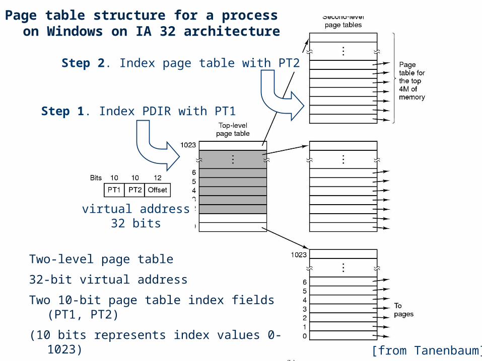
virtual address32 bits
[from Tanenbaum]
Two-level page table
32-bit virtual address
Two 10-bit page table index fields (PT1, PT2)
(10 bits represents index values 0-1023)
Step 1. Index PDIR with PT1
Step 2. Index page table with PT2
Page table structure for a process on Windows on IA 32 architecture
Virtual Address Translation
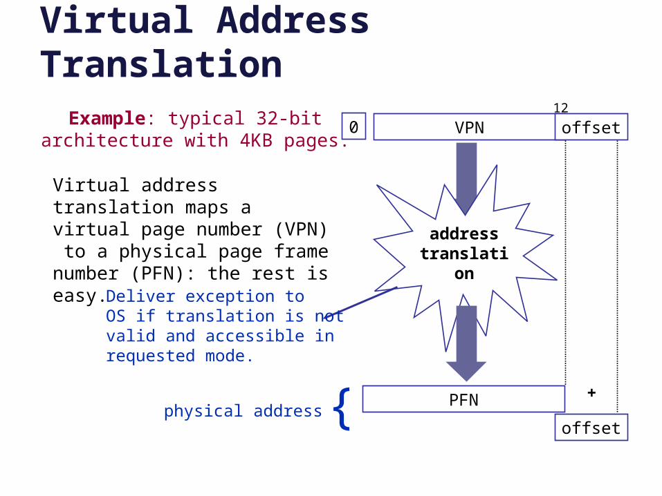
VPN offset12
Example: typical 32-bitarchitecture with 4KB pages.
addresstranslation
Virtual address translation maps a virtual page number (VPN) to a physical page frame number (PFN): the rest is easy.
PFN
offset
+
0
physical address {
Deliver exception toOS if translation is notvalid and accessible inrequested mode.
More pictures
• We did not discuss these last three pictures to help understand name mapping structures.
• COW: one advantage of page/block maps is that it becomes easy to clone (logical copy) a block space.– Copy a storage object P to make a new object C. P could be a
file, segment, volume, or virtual address space (for fork!).
– Copy the map P: make a new map C referencing the same blocks. The map copy is cheap: no need to copy the data itself.
– Since a clone is a copy, any changes (writes) to P after the clone should not affect C, and vice versa.
– Use a lazy copy or copy-on-write (COW). Intercept writes (how?) and copy the affected block before executing the write.

Copy on write
Physical memory
Parent memory
Child memory
What happens if parent writes to a page?
Landon Cox
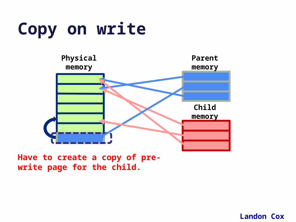
Copy on write
Child memory
Have to create a copy of pre-write page for the child.
Physical memory
Parent memory
Landon Cox
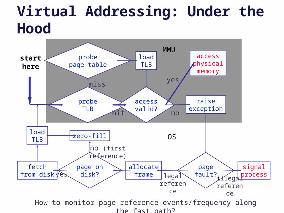
Virtual Addressing: Under the Hood
raiseexception
probepage table
loadTLB
probe TLB
accessphysicalmemory
accessvalid?
pagefault?
signalprocess
allocateframe
page ondisk?
fetchfrom disk
zero-fillloadTLB
starthere
MMU
OS
illegal reference
legal reference
yes
no (first reference)
yes
no
miss
hit
How to monitor page reference events/frequency along the fast path?
Replacement policy: file systems
• File systems often use a variant of LRU.– A file system sees every block access (through syscall API), so it
can do full LRU: move block to tail of LRU list on each access.
• Sequential files have a cache wiping effect with LRU.– Most file systems detect sequential access and prefer eviction of
blocks from the same file, e.g., using MRU.
– That also prevents any one file/object from consuming more than its “fair share” of the cache.
VM systems
• VM memory management is similar to file systems.– Page caching in physical memory frames
– Unified with file block caching in most systems
– Virtual address space is a collection of regions/segments, which may be considered as “objects” similar to files.
• Only it’s different.– Mapped by page tables
– VM system software does not see most references, since they are accelerated by Memory Management Unit hardware.
– Requires a sampling approximation for page replacement.
– All data goes away on a system failure: no write atomicity.
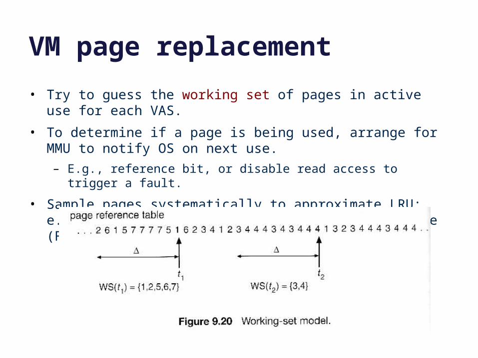
VM page replacement
• Try to guess the working set of pages in active use for each VAS.
• To determine if a page is being used, arrange for MMU to notify OS on next use.
– E.g., reference bit, or disable read access to trigger a fault.
• Sample pages systematically to approximate LRU: e.g., CLOCK algorithm, or FIFO-with-Second-Chance (FIFO-2C)
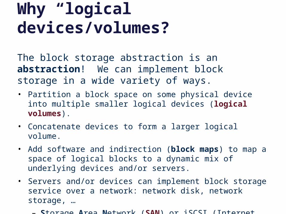
Why “logical” devices/volumes?
The block storage abstraction is an abstraction! We can implement block storage in a wide variety of ways. • Partition a block space on some physical device into multiple
smaller logical devices (logical volumes).
• Concatenate devices to form a larger logical volume.
• Add software and indirection (block maps) to map a space of logical blocks to a dynamic mix of underlying devices and/or servers.
• Servers and/or devices can implement block storage service over a network: network disk, network storage, …
– Storage Area Network (SAN) or iSCSI (Internet SCSI).
– Network-Attached Storage (NAS) generally refers to a network file system abstraction, built above block storage.
• Add another level of indirection! Storage virtualization.
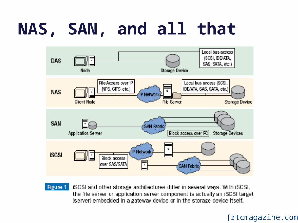
[rtcmagazine.com]
NAS, SAN, and all that
File Systems and StorageDay Three
Performance and Reliability
Jeff ChaseDuke University
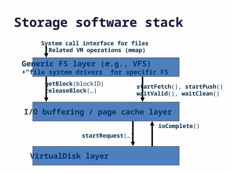
Generic FS layer (e.g., VFS)+“file system drivers” for specific FS
VirtualDisk layer
startRequest(…)
ioComplete()
startFetch(), startPush()waitValid(), waitClean()
getBlock(blockID)releaseBlock(…)
System call interface for filesRelated VM operations (mmap)
Storage software stack
I/O buffering / page cache layer
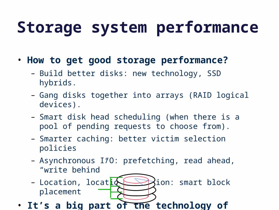
Storage system performance
• How to get good storage performance?– Build better disks: new technology, SSD hybrids.
– Gang disks together into arrays (RAID logical devices).
– Smart disk head scheduling (when there is a pool of pending requests to choose from).
– Smarter caching: better victim selection policies
– Asynchronous I/O: prefetching, read ahead, “write behind”
– Location, location, location: smart block placement
• It’s a big part of the technology of storage systems.
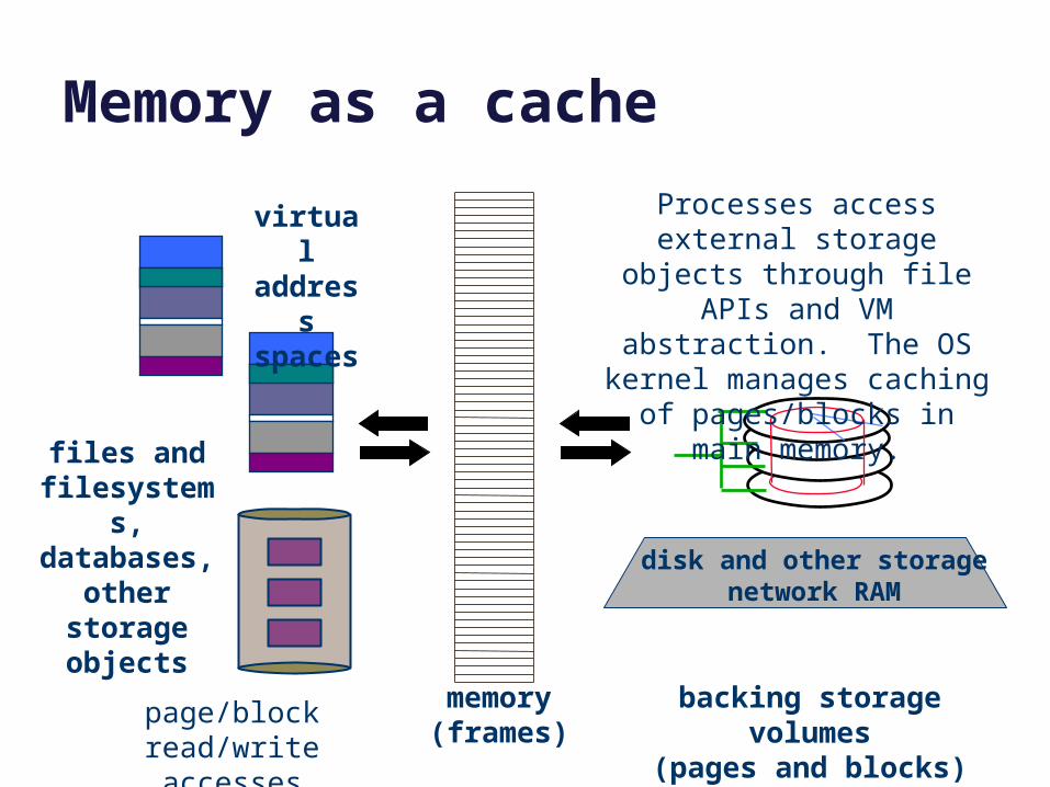
Memory as a cache
memory(frames)
data
data
virtual address spaces
files and filesystems,databases,
other storage objects
disk and other storagenetwork RAM
page/block read/write accesses
backing storage volumes(pages and blocks)
Processes access external storage objects through file
APIs and VM abstraction. The OS kernel manages caching
of pages/blocks in main memory.
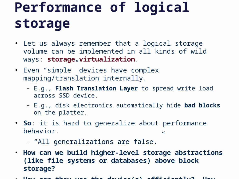
Performance of logical storage• Let us always remember that a logical storage volume can be
implemented in all kinds of wild ways: storage virtualization.
• Even “simple” devices have complex mapping/translation internally.
– E.g., Flash Translation Layer to spread write load across SSD device.
– E.g., disk electronics automatically hide bad blocks on the platter.
• So: it is hard to generalize about performance behavior.
– “All generalizations are false.”
• How can we build higher-level storage abstractions (like file systems or databases) above block storage?
• How can they use the device(s) efficiently? How much do they need to know about storage performance properties?
– E.g., “seeks waste time”
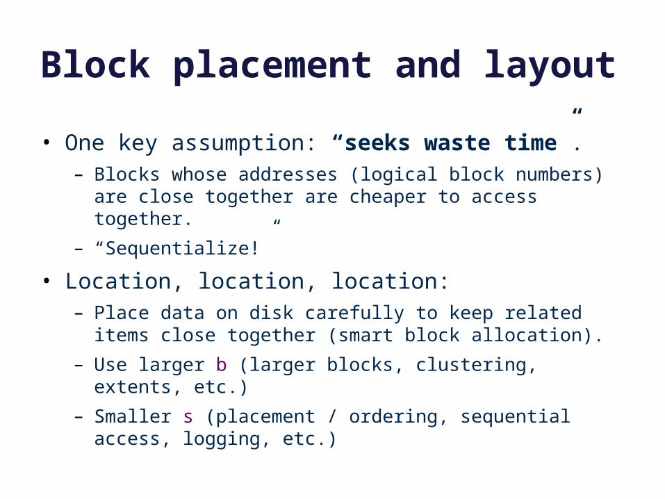
Block placement and layout
• One key assumption: “seeks waste time”.– Blocks whose addresses (logical block numbers) are close
together are cheaper to access together.
– “Sequentialize!”
• Location, location, location:– Place data on disk carefully to keep related items close together
(smart block allocation).
– Use larger b (larger blocks, clustering, extents, etc.)
– Smaller s (placement / ordering, sequential access, logging, etc.)
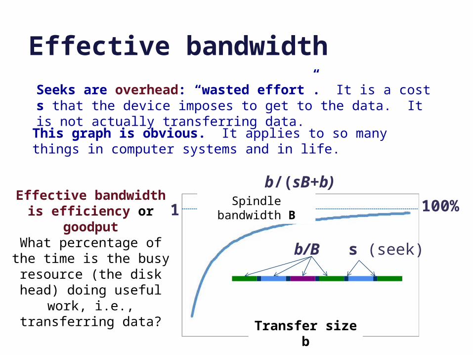
Effective bandwidth
Transfer size b
Effective bandwidth is efficiency or goodputWhat percentage of the
time is the busy resource (the disk head) doing useful work, i.e., transferring data?
b/(sB+b)
b/B s (seek)
1 100%
Seeks are overhead: “wasted effort”. It is a cost s that the device imposes to get to the data. It is not actually transferring data.
This graph is obvious. It applies to so many things in computer systems and in life.
Spindle bandwidth B
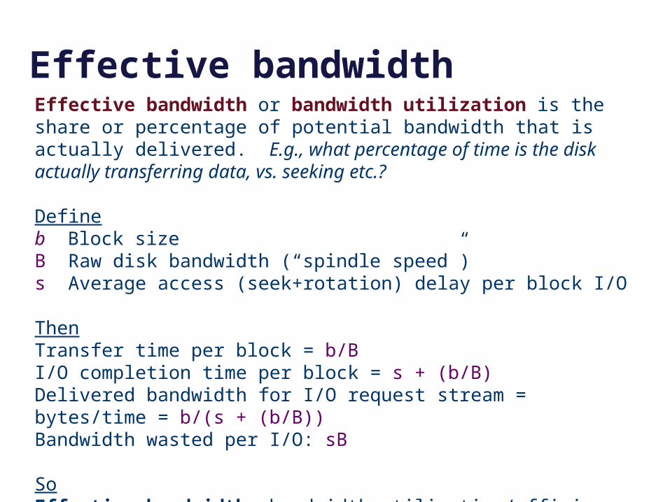
Effective bandwidthEffective bandwidth or bandwidth utilization is the share or percentage of potential bandwidth that is actually delivered. E.g., what percentage of time is the disk actually transferring data, vs. seeking etc.?
Defineb Block sizeB Raw disk bandwidth (“spindle speed”)s Average access (seek+rotation) delay per block I/O
ThenTransfer time per block = b/BI/O completion time per block = s + (b/B)Delivered bandwidth for I/O request stream = bytes/time = b/(s + (b/B))Bandwidth wasted per I/O: sB
SoEffective bandwidth: bandwidth utilization/efficiency (%): b/(sB + b)[bytes transferred over the “byte time slots” consumed for the transfer]
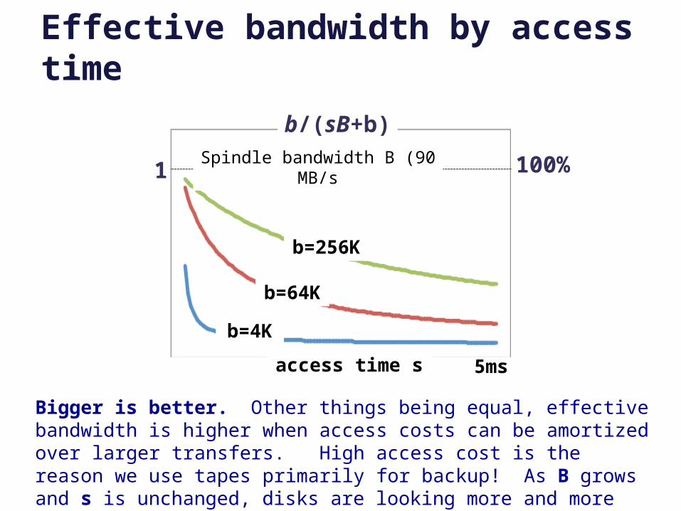
Effective bandwidth by access time
b/(sB+b)
1 100%Spindle bandwidth B (90 MB/s
access time s 5ms
b=256K
b=64K
b=4K
Bigger is better. Other things being equal, effective bandwidth is higher when access costs can be amortized over larger transfers. High access cost is the reason we use tapes primarily for backup! As B grows and s is unchanged, disks are looking more and more like tapes! (Jim Gray)
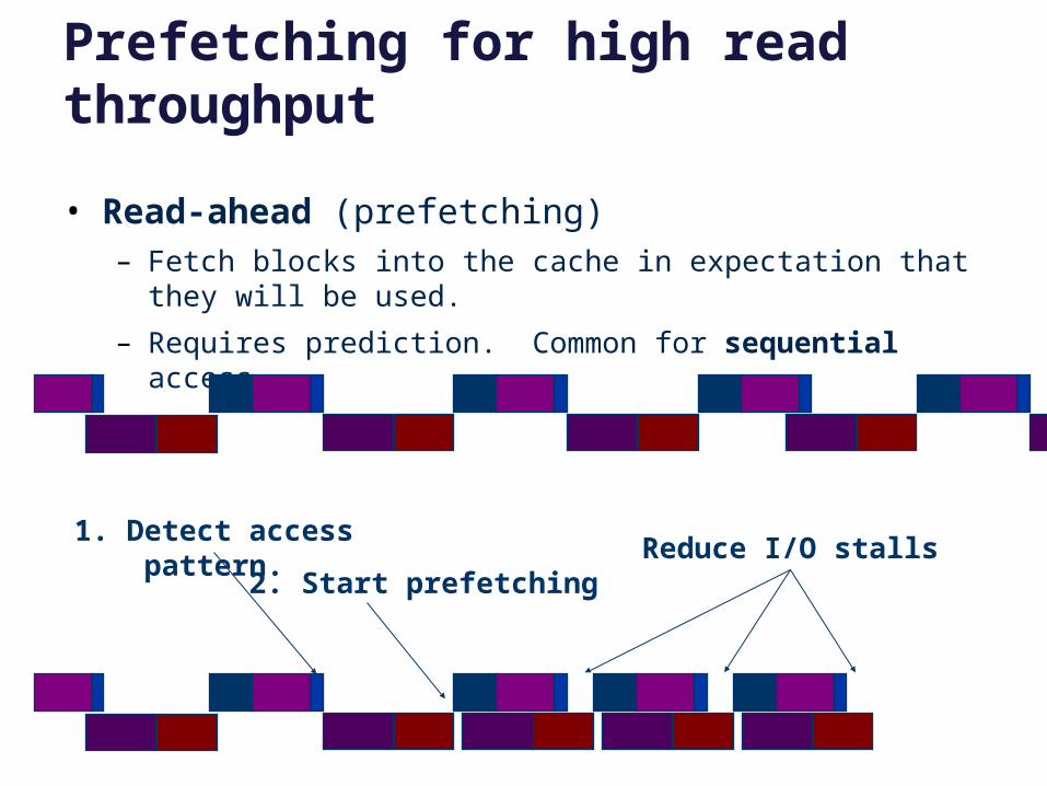
Prefetching for high read throughput
• Read-ahead (prefetching)– Fetch blocks into the cache in expectation that they will be used.
– Requires prediction. Common for sequential access.
1. Detect access pattern.
2. Start prefetchingReduce I/O stalls
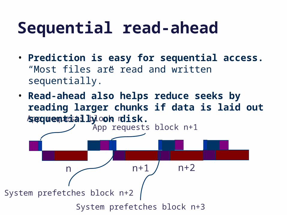
Sequential read-ahead
n n+1
App requests block nApp requests block n+1
n+2
System prefetches block n+2
System prefetches block n+3
• Prediction is easy for sequential access. “Most files are read and written sequentially.”
• Read-ahead also helps reduce seeks by reading larger chunks if data is laid out sequentially on disk.
Building better file systems
• The 1990s was a period of experimentation with new strategies for high-performance file system design.
• The new file systems generally used the FFS mechanisms and data structures, but changed the policies for block allocation.
– Block allocation policy: where to place new data (or modified old data) on the storage volume? Which block number to choose?
– “File system design is 99% block allocation.” - Larry McVoy
– Example: Group large-file data into big contiguous chunks called clusters or extents that can be read or written as a unit (larger b). [McVoy91] and [Smith/Seltzer96]
– Example: Write modified data and metadata wherever convenient to minimize seeking: e.g., “log-structured” file systems (LFS) [Rosenblum91] and NetApp’s WAFL [Hitz95]. Note: requires a level of indirection so the FS can write each version of an inode to a different location on the disk. (See WAFL’s inode file.)
Fast File System (FFS)
• Fast File System (FFS) [McKusick81] is the historical, canonical Unix file system that actually works.
• In the old days (1970s-1980s), file systems delivered only 10% of the available disk bandwidth, even on the old disks.
• FFS extended the classic 1970s Unix file system design with a new focus on performance in the Berkeley Unix release (BSD: 1982).
– Multiple block sizes: use small blocks called frags in small files, to reduce internal fragmentation.
– Smart block allocation that pays attention to disk locality by placing data/metadata in zones called cylinder groups.
• FFS was still lousy, but it laid the groundwork for development of high-performance file systems over the next 20 years.
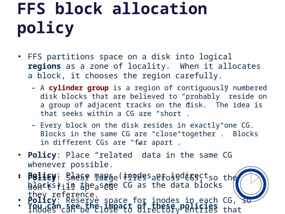
FFS block allocation policy
• FFS partitions space on a disk into logical regions as a zone of locality. When it allocates a block, it chooses the region carefully.
– A cylinder group is a region of contiguously numbered disk blocks that are believed to “probably” reside on a group of adjacent tracks on the disk. The idea is that seeks within a CG are “short”.
– Every block on the disk resides in exactly one CG. Blocks in the same CG are “close together”. Blocks in different CGs are “far apart”.
• Policy: Place “related” data in the same CG whenever possible.
• Policy: Smear large files across CGs, so they don’t fill up a CG.
• Policy: Reserve space for inodes in each CG, so inodes can be close to directory entries that reference them.
• Policy: Place maps (inodes or indirect blocks) in the same CG as the data blocks they reference.
• You can see the impact of these policies in the plots!
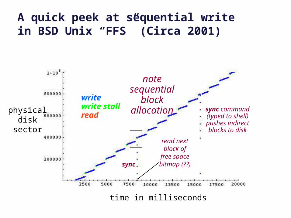
A quick peek at sequential writein BSD Unix “FFS” (Circa 2001)
physicaldisk
sector
time in milliseconds
writewrite stallread
sync command(typed to shell)pushes indirectblocks to disk
read nextblock of
free spacebitmap (??)
note sequential block allocation
sync
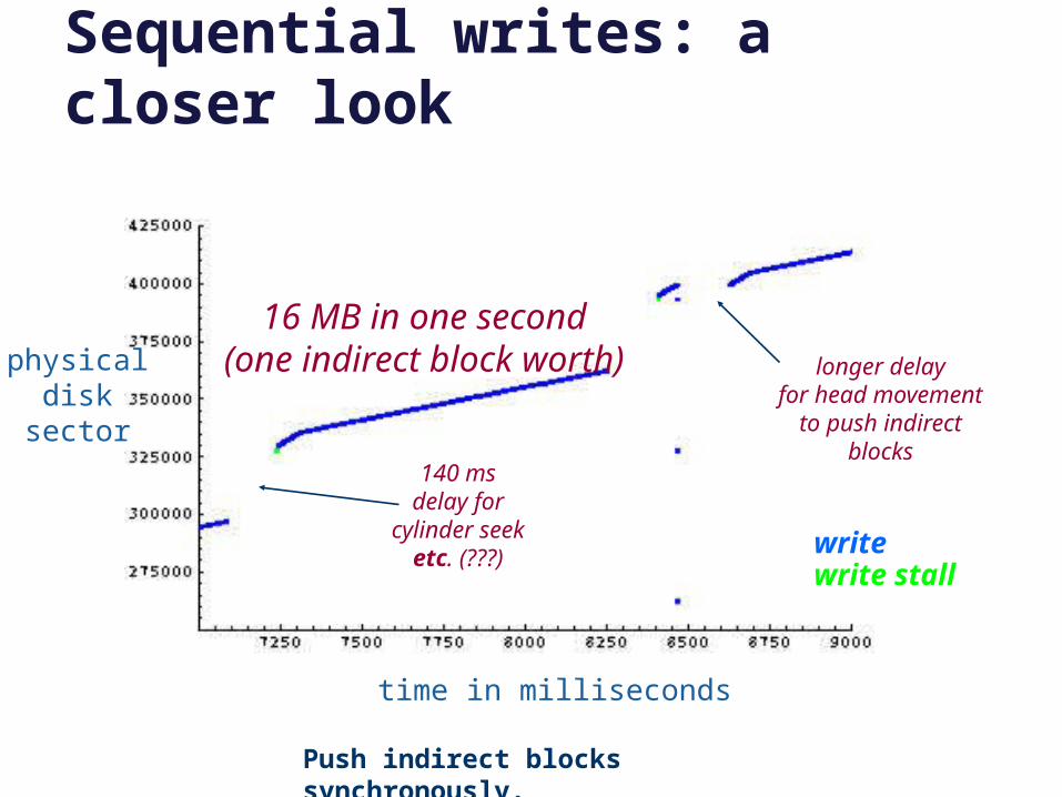
Sequential writes: a closer look
writewrite stall
140 msdelay for
cylinder seeketc. (???)
longer delayfor head movement
to push indirectblocks
16 MB in one second(one indirect block worth)
time in milliseconds
physicaldisk
sector
Push indirect blocks synchronously.
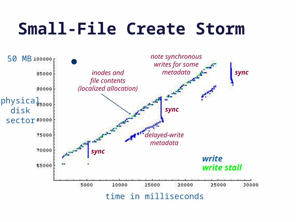
Small-File Create Storm
writewrite stall
time in milliseconds
physicaldisk
sector
sync
sync
syncinodes andfile contents
(localized allocation)
delayed-writemetadata
note synchronouswrites for some
metadata
50 MB
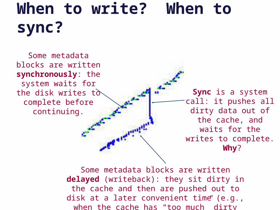
When to write? When to sync?
Some metadata blocks are written
synchronously: the system waits for the disk writes to complete before
continuing.
Some metadata blocks are written delayed (writeback): they sit dirty in the cache and then are pushed out to disk at a later convenient time (e.g.,
when the cache has “too much” dirty data).
Sync is a system call: it pushes all dirty data out of the cache, and waits
for the writes to complete. Why?
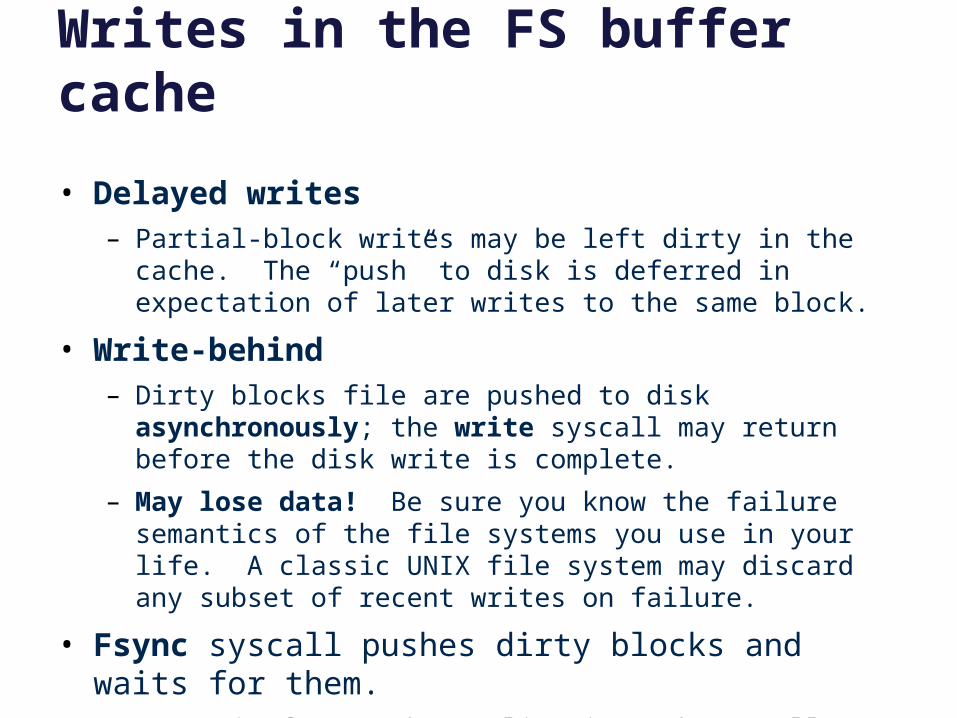
Writes in the FS buffer cache
• Delayed writes– Partial-block writes may be left dirty in the cache. The “push” to
disk is deferred in expectation of later writes to the same block.
• Write-behind– Dirty blocks file are pushed to disk asynchronously; the write
syscall may return before the disk write is complete.
– May lose data! Be sure you know the failure semantics of the file systems you use in your life. A classic UNIX file system may discard any subset of recent writes on failure.
• Fsync syscall pushes dirty blocks and waits for them.– Fsync is for use by applications that really want to know their
data is “safe”. Good file systems implicitly fsync-on-close.
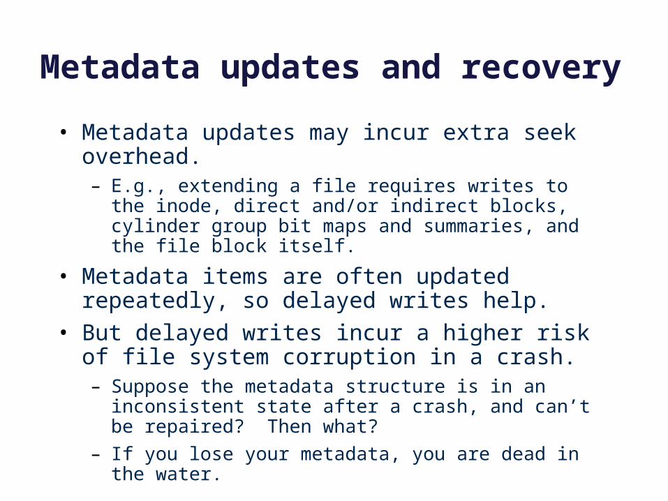
Metadata updates and recovery
• Metadata updates may incur extra seek overhead.– E.g., extending a file requires writes to the inode, direct
and/or indirect blocks, cylinder group bit maps and summaries, and the file block itself.
• Metadata items are often updated repeatedly, so delayed writes help.
• But delayed writes incur a higher risk of file system corruption in a crash.– Suppose the metadata structure is in an inconsistent state
after a crash, and can’t be repaired? Then what?
– If you lose your metadata, you are dead in the water.
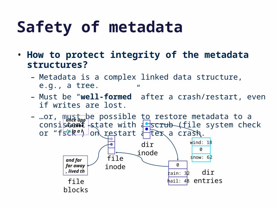
Safety of metadata
• How to protect integrity of the metadata structures?– Metadata is a complex linked data structure, e.g., a tree.
– Must be “well-formed” after a crash/restart, even if writes are lost.
– …or, must be possible to restore metadata to a consistent state with a scrub (file system check or “fsck”) on restart after a crash.
0
rain: 32
hail: 48
once upon a time/n in a l
and far far away, lived th
file inode
0
wind: 18
snow: 62
dir inode
dir entriesfile blocks
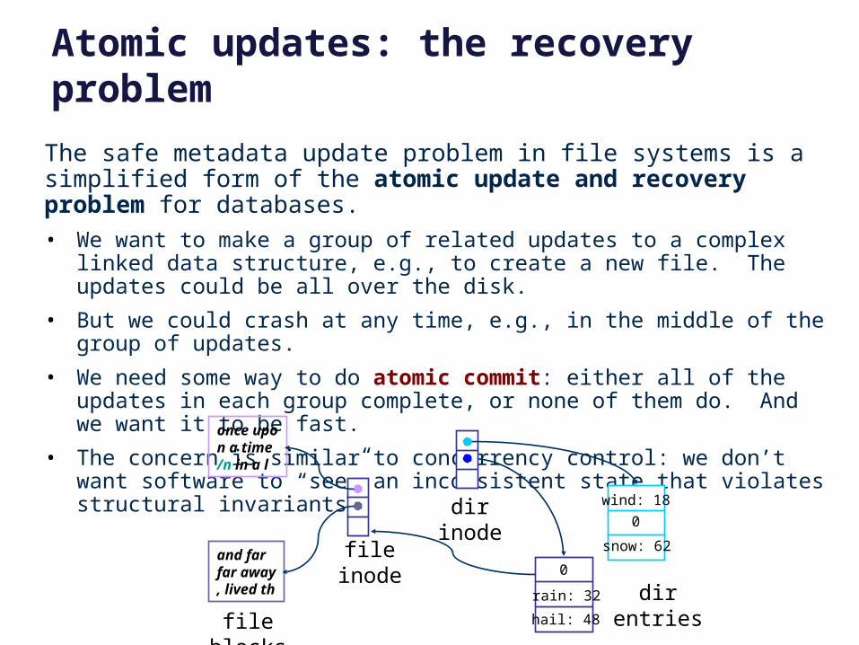
Atomic updates: the recovery problem
The safe metadata update problem in file systems is a simplified form of the atomic update and recovery problem for databases.
• We want to make a group of related updates to a complex linked data structure, e.g., to create a new file. The updates could be all over the disk.
• But we could crash at any time, e.g., in the middle of the group of updates.
• We need some way to do atomic commit: either all of the updates in each group complete, or none of them do. And we want it to be fast.
• The concern is similar to concurrency control: we don’t want software to “see” an inconsistent state that violates structural invariants.
0
rain: 32
hail: 48
once upon a time/n in a l
and far far away, lived th
file inode
0
wind: 18
snow: 62
dir inode
dir entriesfile blocks
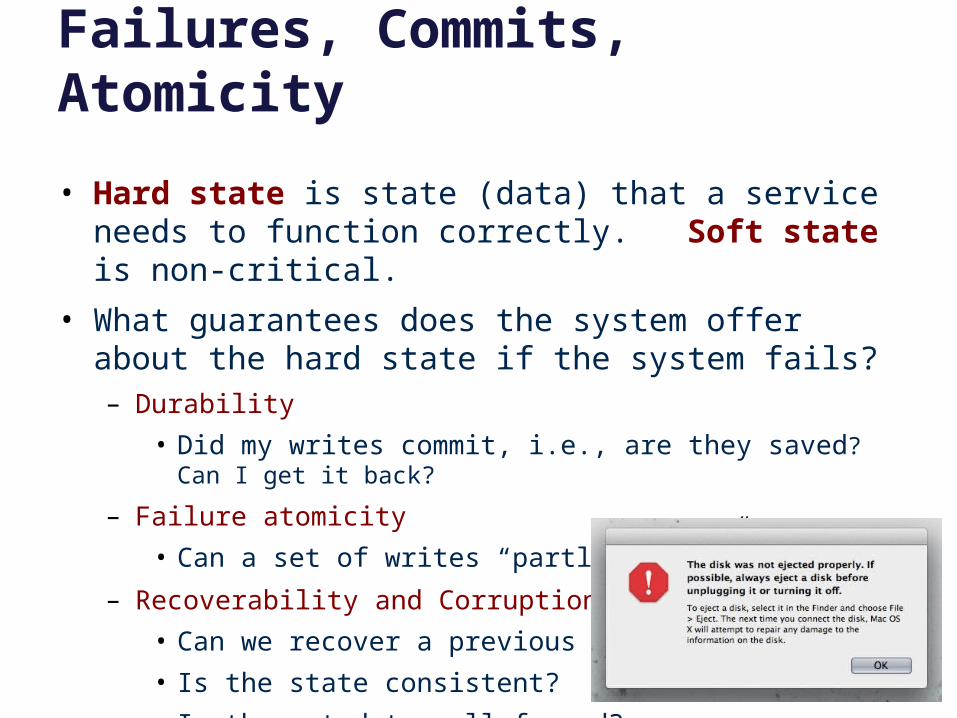
Failures, Commits, Atomicity
• Hard state is state (data) that a service needs to function correctly. Soft state is non-critical.
• What guarantees does the system offer about the hard state if the system fails?– Durability
• Did my writes commit, i.e., are they saved? Can I get it back?
– Failure atomicity
• Can a set of writes “partly commit”?
– Recoverability and Corruption
• Can we recover a previous state?
• Is the state consistent?
• Is the metadata well-formed?
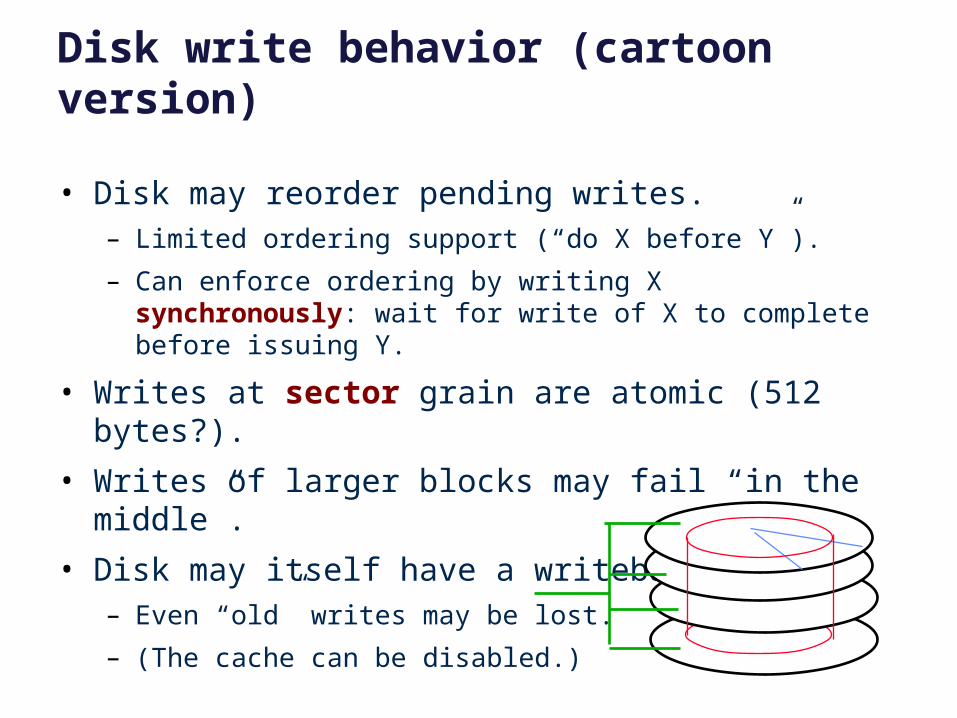
Disk write behavior (cartoon version)
• Disk may reorder pending writes.– Limited ordering support (“do X before Y”).
– Can enforce ordering by writing X synchronously: wait for write of X to complete before issuing Y.
• Writes at sector grain are atomic (512 bytes?).
• Writes of larger blocks may fail “in the middle”.
• Disk may itself have a writeback cache.– Even “old” writes may be lost.
– (The cache can be disabled.)

Atomic commit: techniques
We consider three three techniques for atomic commit and recovery, in the context of file systems.
• Option 1: careful write ordering, with scrub on recovery
• Option 2: logging/journaling (also used in databases)
• Option 3: shadowing (e.g., WAFL)
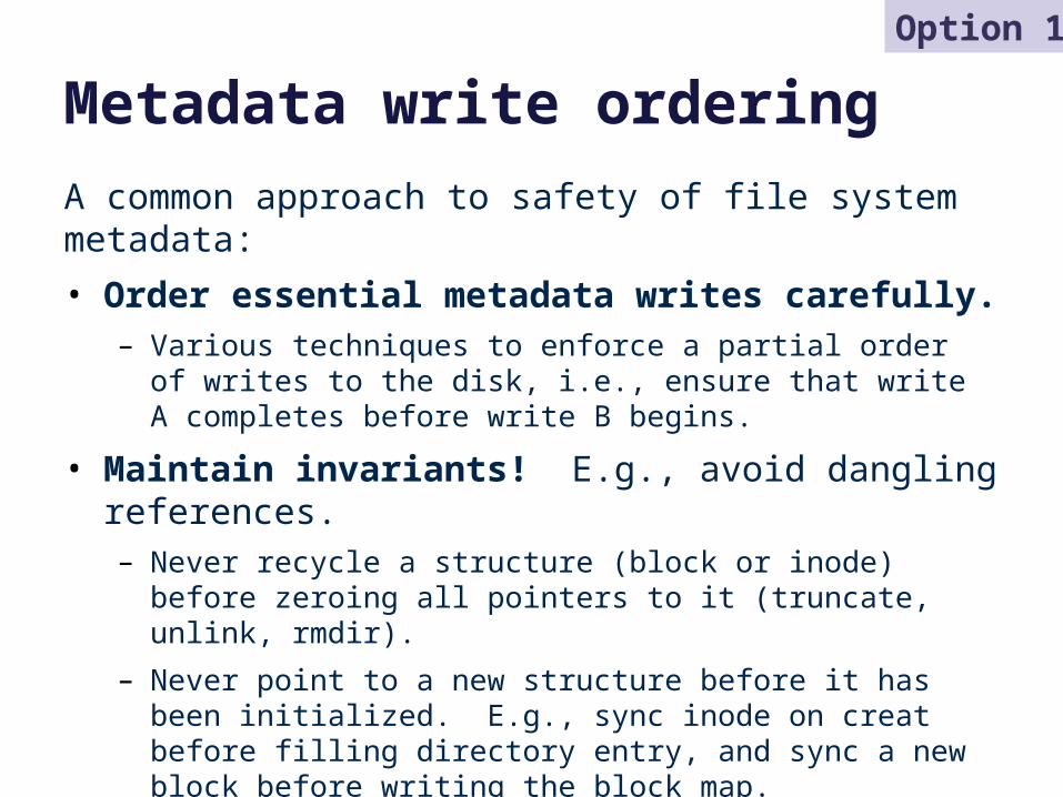
Metadata write ordering
A common approach to safety of file system metadata:
• Order essential metadata writes carefully.– Various techniques to enforce a partial order of writes to the
disk, i.e., ensure that write A completes before write B begins.
• Maintain invariants! E.g., avoid dangling references.– Never recycle a structure (block or inode) before zeroing all
pointers to it (truncate, unlink, rmdir).
– Never point to a new structure before it has been initialized. E.g., sync inode on creat before filling directory entry, and sync a new block before writing the block map.
• Traverse the metadata tree to rebuild derived structures.– Post-crash scrub can rebuild/repair other structures e.g., free
block bitmaps, free inode bitmaps.
Option 1
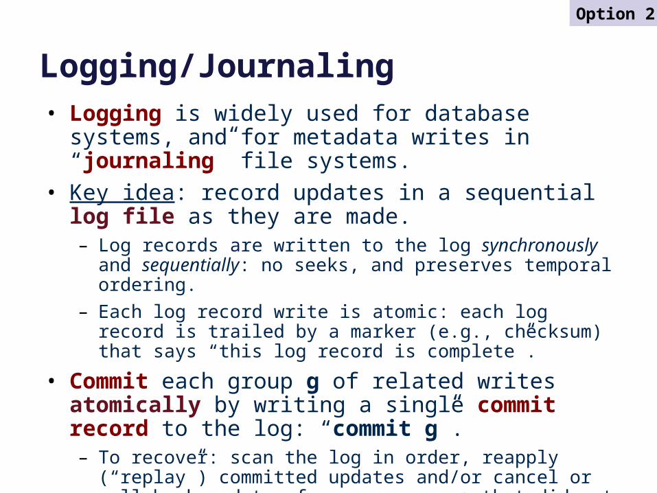
Logging/Journaling• Logging is widely used for database systems, and for
metadata writes in “journaling” file systems.
• Key idea: record updates in a sequential log file as they are made. – Log records are written to the log synchronously and
sequentially: no seeks, and preserves temporal ordering.
– Each log record write is atomic: each log record is trailed by a marker (e.g., checksum) that says “this log record is complete”.
• Commit each group g of related writes atomically by writing a single commit record to the log: “commit g”.– To recover: scan the log in order, reapply (“replay”) committed
updates and/or cancel or roll back updates from any group g that did not commit before the crash.
Option 2
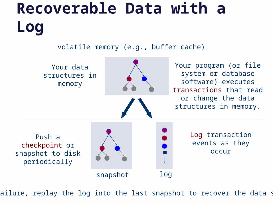
Recoverable Data with a Logvolatile memory (e.g., buffer cache)
logsnapshot
Your program (or file system or database software)
executes transactions that read or change the data structures in memory.
Your data structures in memory
Push a checkpoint or snapshot to disk
periodically
Log transaction events as they occur
After a failure, replay the log into the last snapshot to recover the data structure.
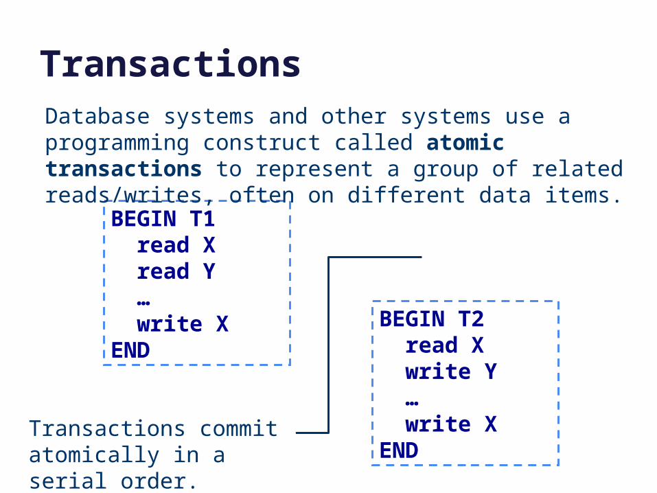
Transactions
BEGIN T1 read X read Y … write XEND
Database systems and other systems use a programming construct called atomic transactions to represent a group of related reads/writes, often on different data items.
BEGIN T2 read X write Y … write XEND
Transactions commit atomically in a serial order.
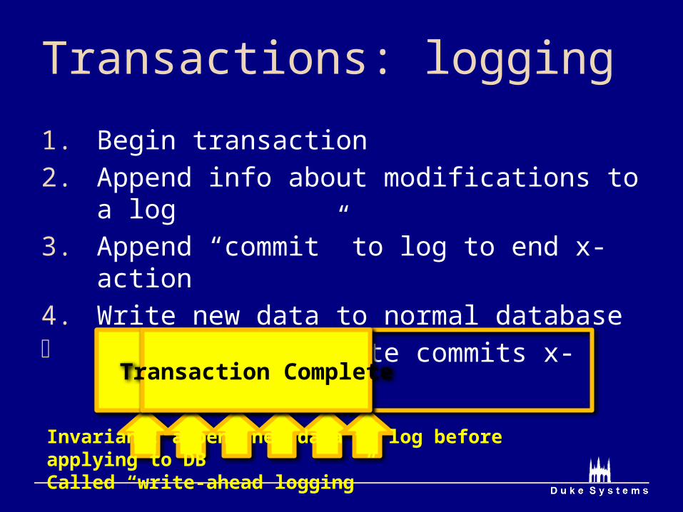
Transactions: logging
1. Begin transaction2. Append info about modifications to a log3. Append “commit” to log to end x-action4. Write new data to normal database Single-sector write commits x-action (3)
Invariant: append new data to log before applying to DBCalled “write-ahead logging”
Begi
n
Writ
e1
…
Writ
eN
Com
mit
Transaction Complete
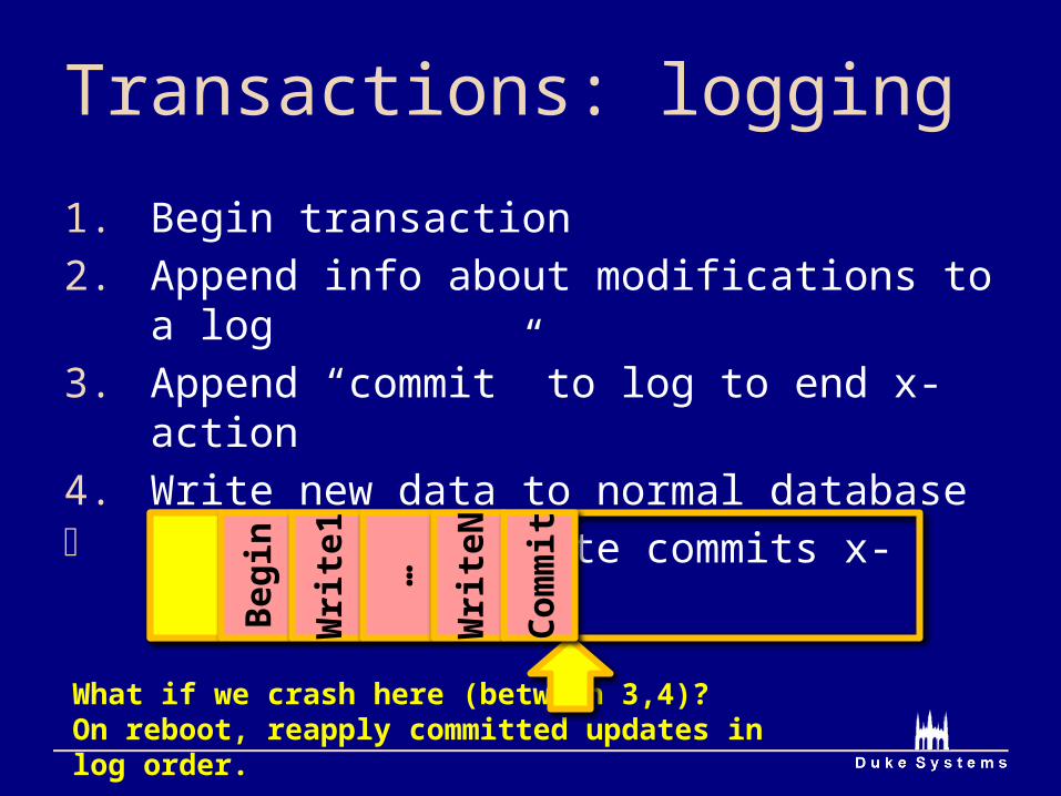
Transactions: logging
1. Begin transaction2. Append info about modifications to a log3. Append “commit” to log to end x-action4. Write new data to normal database Single-sector write commits x-action (3)
What if we crash here (between 3,4)?On reboot, reapply committed updates in log order.
Begi
n
Writ
e1
…
Writ
eN
Com
mit
Transactions: logging
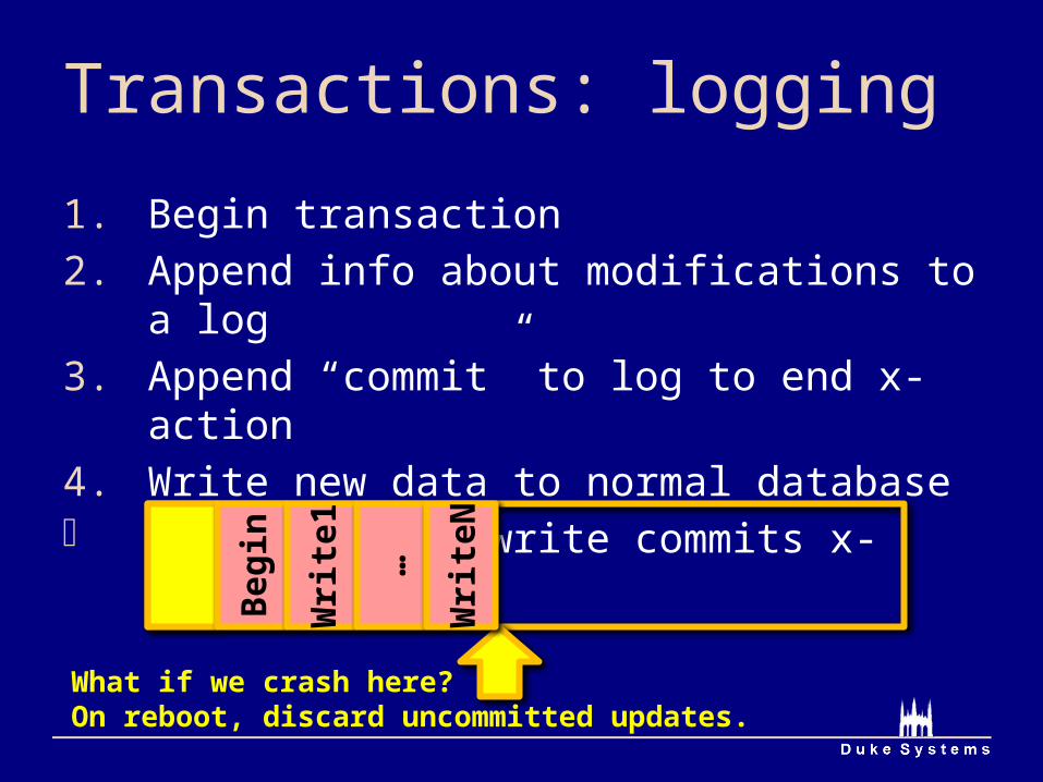
1. Begin transaction2. Append info about modifications to a log3. Append “commit” to log to end x-action4. Write new data to normal database Single-sector write commits x-action (3)
What if we crash here?On reboot, discard uncommitted updates.
Begi
n
Writ
e1
…
Writ
eN
Anatomy of a Log
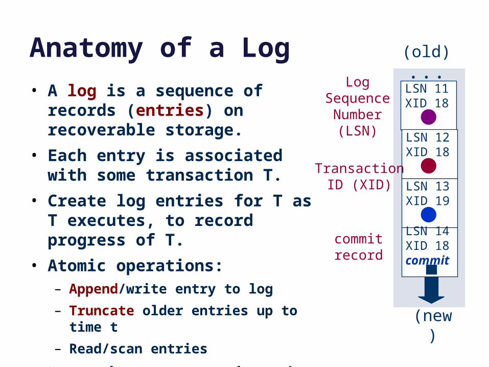
• A log is a sequence of records (entries) on recoverable storage.
• Each entry is associated with some transaction T.
• Create log entries for T as T executes, to record progress of T.
• Atomic operations:– Append/write entry to log
– Truncate older entries up to time t
– Read/scan entries
• Log writes are atomic and durable, and complete detectably in order.
(old)
(new)
LSN 11XID 18
LSN 13XID 19
LSN 12XID 18
LSN 14XID 18commit
...Log
SequenceNumber(LSN)
TransactionID (XID)
commitrecord
Using a Log
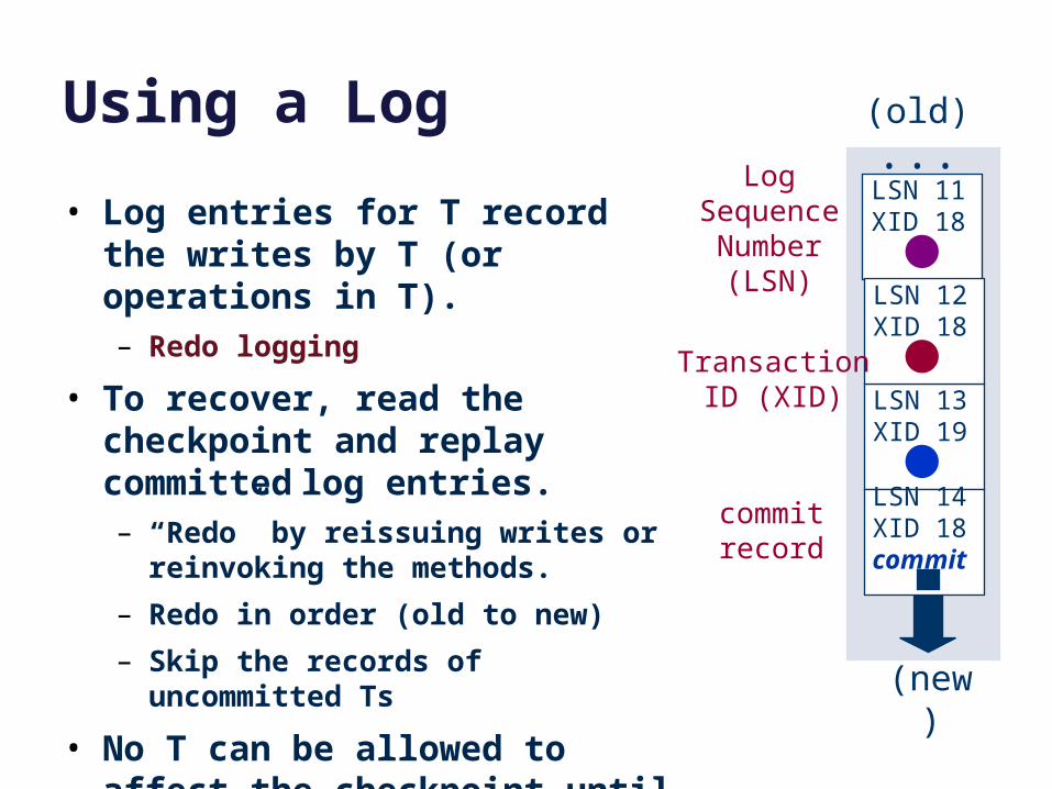
• Log entries for T record the writes by T (or operations in T).– Redo logging
• To recover, read the checkpoint and replay committed log entries. – “Redo” by reissuing writes or
reinvoking the methods.
– Redo in order (old to new)
– Skip the records of uncommitted Ts
• No T can be allowed to affect the checkpoint until T commits.– Technique: write-ahead logging
(old)
(new)
LSN 11XID 18
LSN 13XID 19
LSN 12XID 18
LSN 14XID 18commit
...Log
SequenceNumber(LSN)
TransactionID (XID)
commitrecord
Managing a Log
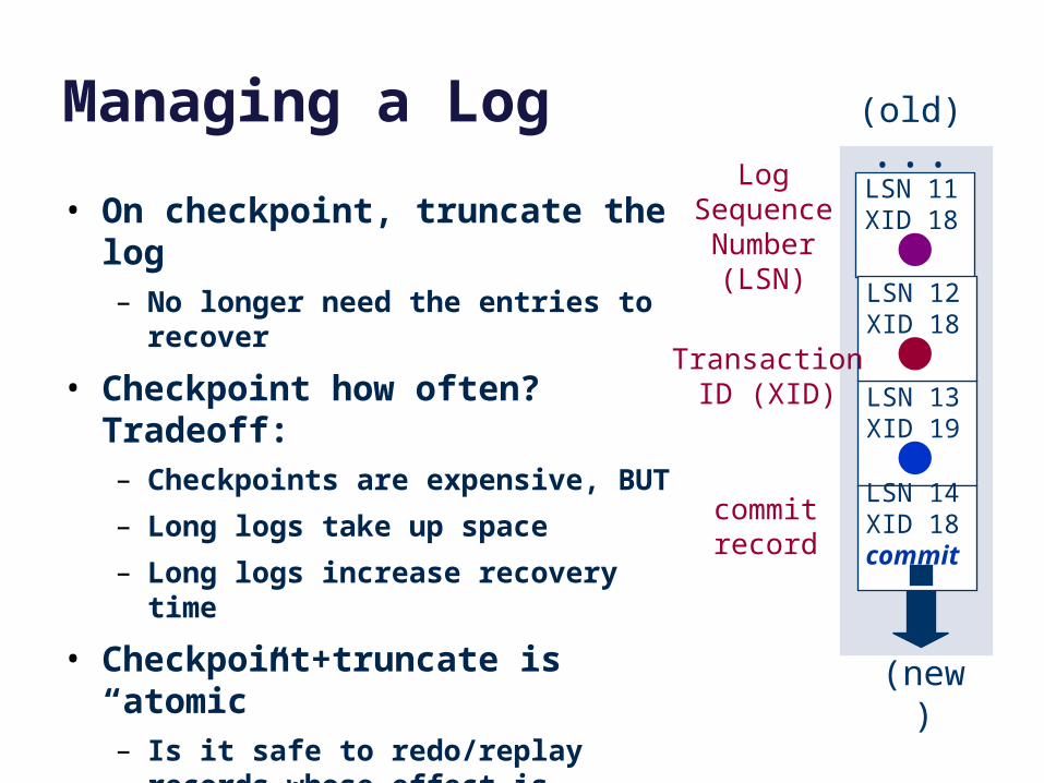
• On checkpoint, truncate the log– No longer need the entries to recover
• Checkpoint how often? Tradeoff:– Checkpoints are expensive, BUT
– Long logs take up space
– Long logs increase recovery time
• Checkpoint+truncate is “atomic”– Is it safe to redo/replay records whose
effect is already in the checkpoint?
– Checkpoint “between” transactions, so checkpoint is a consistent state.
– Lots of approaches
(old)
(new)
LSN 11XID 18
LSN 13XID 19
LSN 12XID 18
LSN 14XID 18commit
...Log
SequenceNumber(LSN)
TransactionID (XID)
commitrecord
File Systems and StorageDay Four
Filers and Service Performance
Jeff ChaseDuke University

Atomic updates: the recovery problem
The safe metadata update problem in file systems is a simplified form of the atomic update and recovery problem for databases.
• We want to make a group of related updates to a complex linked data structure, e.g., to create a new file. The updates could be all over the disk.
• But we could crash at any time, e.g., in the middle of the group of updates.
• We need some way to do atomic commit: either all of the updates in each group complete, or none of them do. And we want it to be fast.
• The concern is similar to concurrency control: we don’t want software to “see” an inconsistent state that violates structural invariants.
0
rain: 32
hail: 48
once upon a time/n in a l
and far far away, lived th
file inode
0
wind: 18
snow: 62
dir inode
dir entriesfile blocks
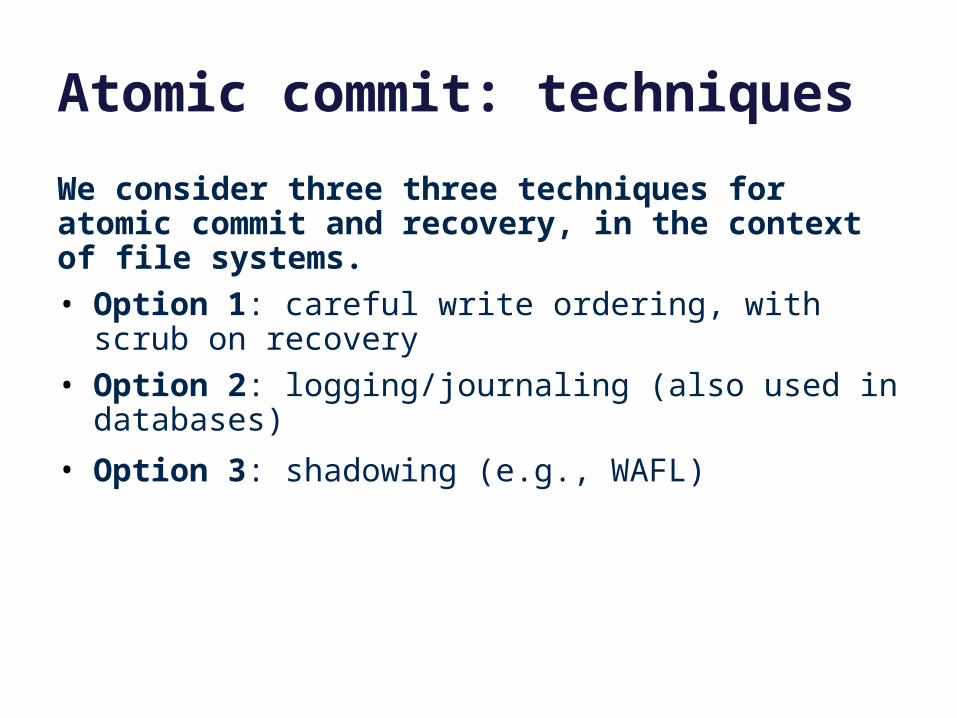
Atomic commit: techniques
We consider three three techniques for atomic commit and recovery, in the context of file systems.
• Option 1: careful write ordering, with scrub on recovery
• Option 2: logging/journaling (also used in databases)
• Option 3: shadowing (e.g., WAFL)
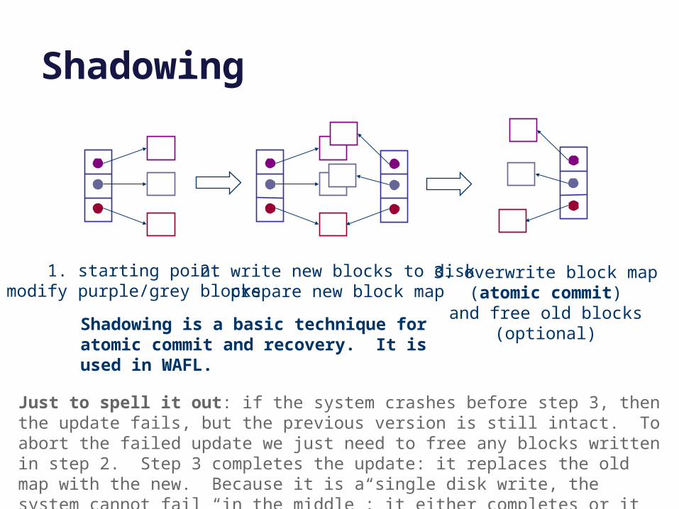
Shadowing
1. starting pointmodify purple/grey blocks
2. write new blocks to diskprepare new block map
3. overwrite block map(atomic commit)
and free old blocks(optional)
Just to spell it out: if the system crashes before step 3, then the update fails, but the previous version is still intact. To abort the failed update we just need to free any blocks written in step 2. Step 3 completes the update: it replaces the old map with the new. Because it is a single disk write, the system cannot fail “in the middle”: it either completes or it does not: it is atomic. Once it is complete, the new data is safe.
Shadowing is a basic technique for atomic commit and recovery. It is used in WAFL.
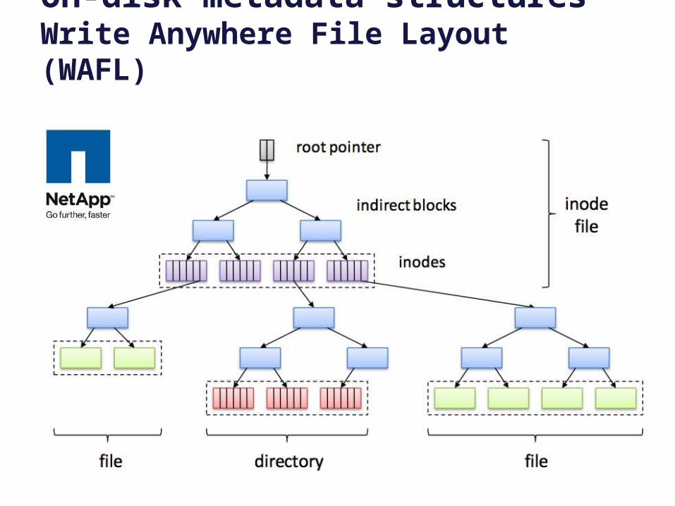
On-disk metadata structures Write Anywhere File Layout (WAFL)
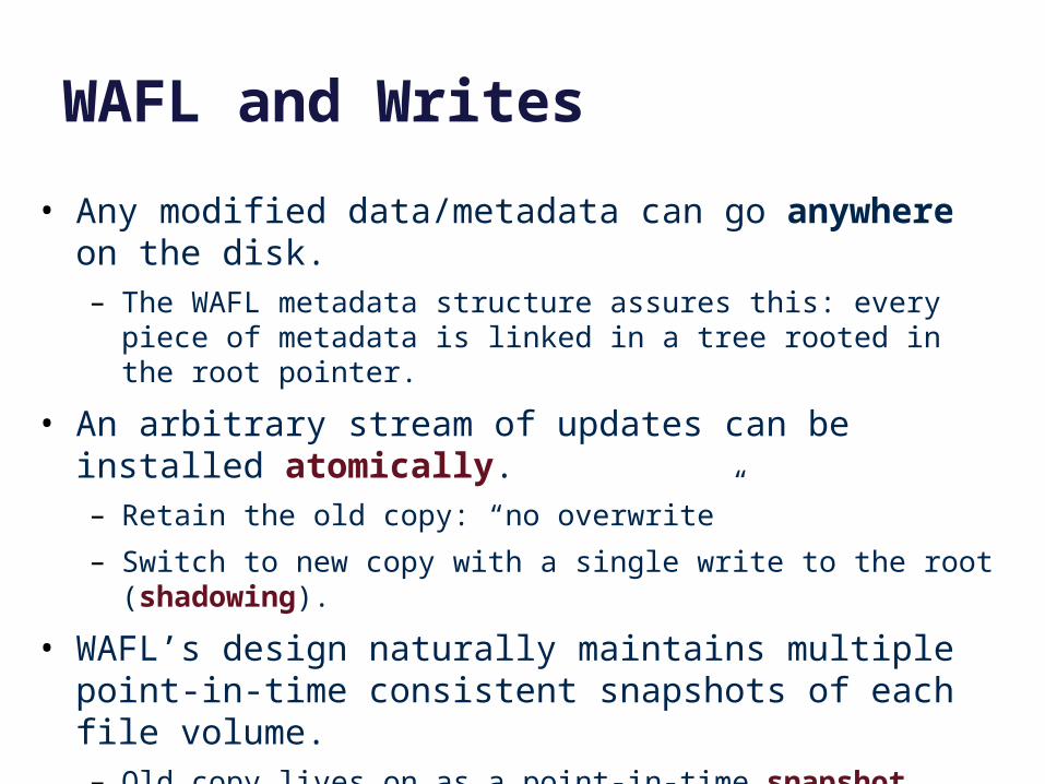
WAFL and Writes
• Any modified data/metadata can go anywhere on the disk.– The WAFL metadata structure assures this: every piece of metadata
is linked in a tree rooted in the root pointer.
• An arbitrary stream of updates can be installed atomically.– Retain the old copy: “no overwrite”
– Switch to new copy with a single write to the root (shadowing).
• WAFL’s design naturally maintains multiple point-in-time consistent snapshots of each file volume.– Old copy lives on as a point-in-time snapshot.
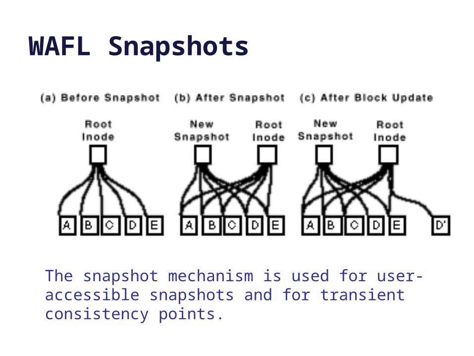
WAFL Snapshots
The snapshot mechanism is used for user-accessible snapshots and for transient consistency points.
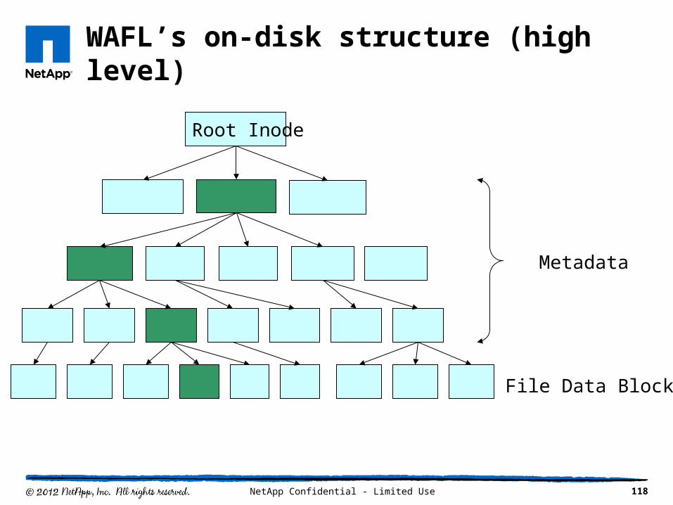
WAFL’s on-disk structure (high level)
118NetApp Confidential - Limited Use
Root Inode
File Data Blocks
Metadata
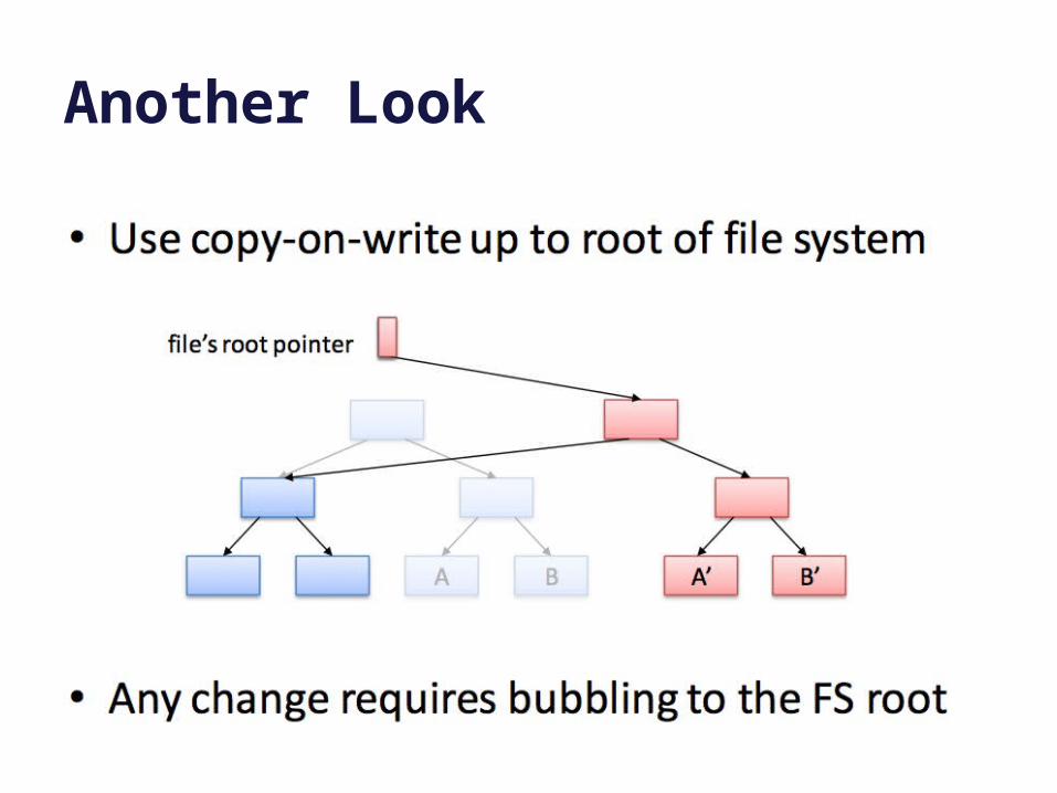
Another Look
WAFL and Performance
• Write the new updated copies wherever and whenever it is “convenient” (fast).
• NetApp filers are designed to be “scalable”: add modules to make the system more powerful.
• E.g., add more disks (RAID).
“Filers”
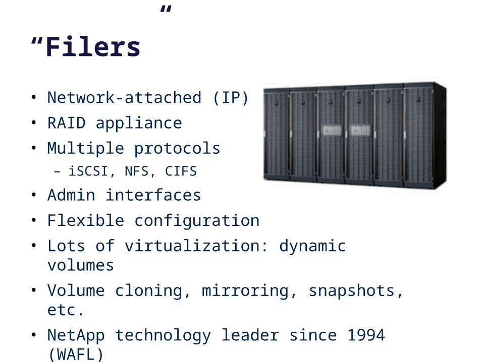
• Network-attached (IP)
• RAID appliance
• Multiple protocols– iSCSI, NFS, CIFS
• Admin interfaces
• Flexible configuration
• Lots of virtualization: dynamic volumes
• Volume cloning, mirroring, snapshots, etc.
• NetApp technology leader since 1994 (WAFL)
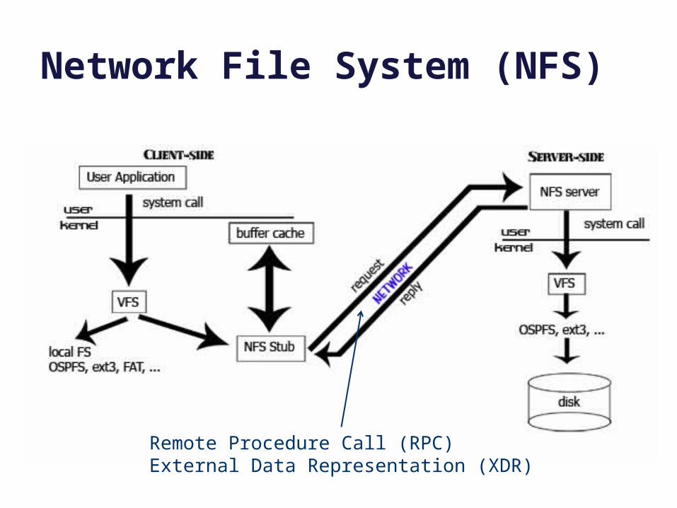
Network File System (NFS)
[ucla.edu]
Remote Procedure Call (RPC)External Data Representation (XDR)
Remote Procedure Call (RPC)
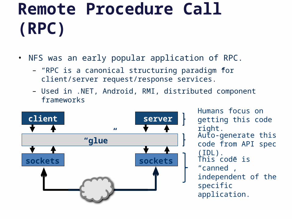
• NFS was an early popular application of RPC.
– “RPC is a canonical structuring paradigm for client/server request/response services.”
– Used in .NET, Android, RMI, distributed component frameworks
client
sockets
server
sockets
“glue”
This code is “canned”, independent of the specific application.
Auto-generate this code from API spec (IDL).
Humans focus on getting this code right.
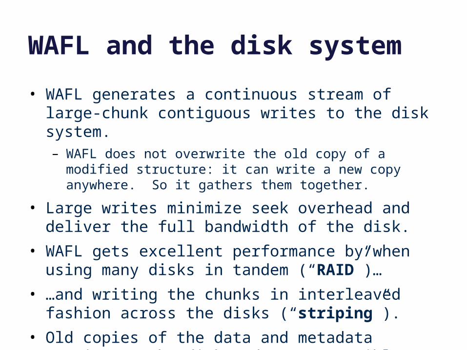
WAFL and the disk system
• WAFL generates a continuous stream of large-chunk contiguous writes to the disk system.– WAFL does not overwrite the old copy of a modified structure: it
can write a new copy anywhere. So it gathers them together.
• Large writes minimize seek overhead and deliver the full bandwidth of the disk.
• WAFL gets excellent performance by/when using many disks in tandem (“RAID”)…
• …and writing the chunks in interleaved fashion across the disks (“striping”).
• Old copies of the data and metadata survive on the disk and are accessible through point-in-time “snapshots”.
Incremental Scalability
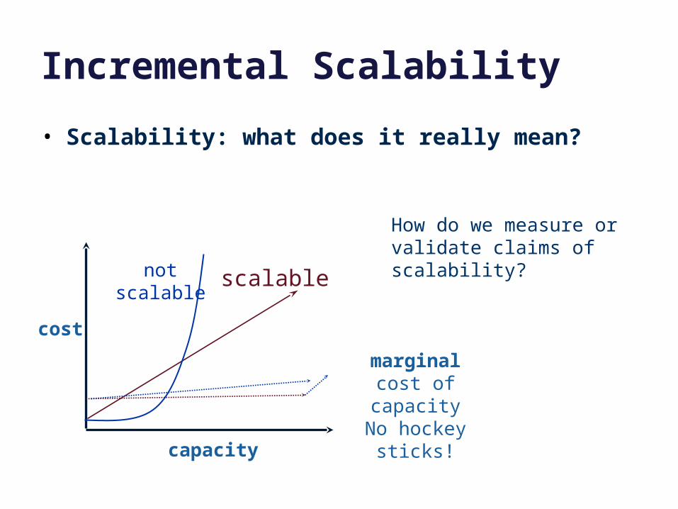
• Scalability: what does it really mean?
cost
capacity
marginalcost of capacity
No hockey sticks!
notscalable
How do we measure or validate claims of scalability?
scalable
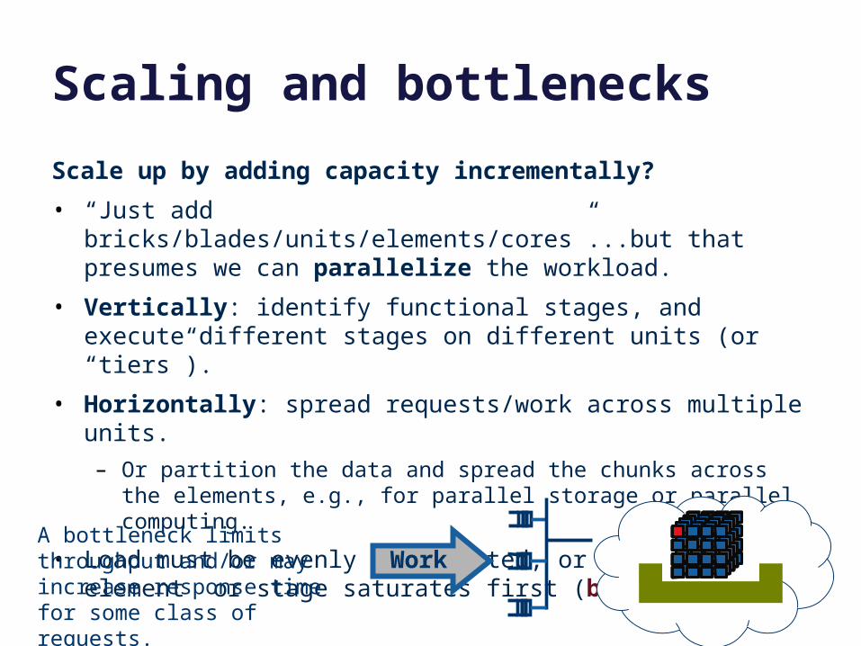
Scaling and bottlenecks
Scale up by adding capacity incrementally?
• “Just add bricks/blades/units/elements/cores”...but that presumes we can parallelize the workload.
• Vertically: identify functional stages, and execute different stages on different units (or “tiers”).
• Horizontally: spread requests/work across multiple units.
– Or partition the data and spread the chunks across the elements, e.g., for parallel storage or parallel computing.
• Load must be evenly distributed, or else some element or stage saturates first (bottleneck).
WorkA bottleneck limits throughput and/or may increase response time for some class of requests.
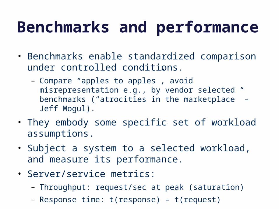
Benchmarks and performance
• Benchmarks enable standardized comparison under controlled conditions.– Compare “apples to apples”, avoid misrepresentation e.g., by
vendor selected benchmarks (“atrocities in the marketplace” – Jeff Mogul).
• They embody some specific set of workload assumptions.
• Subject a system to a selected workload, and measure its performance.
• Server/service metrics:– Throughput: request/sec at peak (saturation)
– Response time: t(response) – t(request)

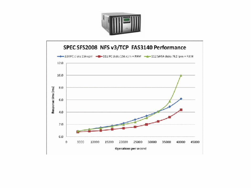
http://www.spec.org/sfs2008/
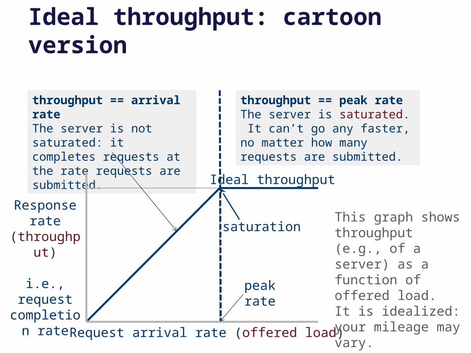
Ideal throughput: cartoon version
Ideal throughput
Request arrival rate (offered load)
Response rate
(throughput)
i.e., request completion
rate
saturation
peak rate
throughput == arrival rateThe server is not saturated: it completes requests at the rate requests are submitted.
throughput == peak rateThe server is saturated. It can’t go any faster, no matter how many requests are submitted.
This graph shows throughput (e.g., of a server) as a function of offered load. It is idealized: your mileage may vary.
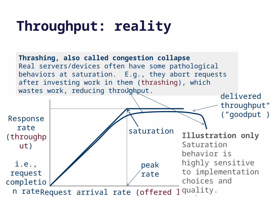
Throughput: reality
Request arrival rate (offered load)
Response rate
(throughput)
i.e., request completion
rate
saturation
peak rate
Thrashing, also called congestion collapseReal servers/devices often have some pathological behaviors at saturation. E.g., they abort requests after investing work in them (thrashing), which wastes work, reducing throughput.
delivered throughput(“goodput”)
Illustration onlySaturation behavior is highly sensitive to implementation choices and quality.
Improving throughput
1. Make the service center faster. (“scale up”)– Upgrade the hardware, spend more $$$
2. Reduce the work required per request (D).– More/smarter caching, code path optimizations, use smarter
disk layout.
3. Add service centers, expand capacity. (“scale out”)– RAIDs, blades, clusters, elastic provisioning
– N centers improves throughput by a factor of N: iff we can partition the workload evenly across the centers!
– Note: the math is different for multiple service centers, and there are various ways to distribute work among them, but we can “squint” and model a balanced aggregate roughly as a single service center: the cartoon graphs still work.

Measuredthroughput(“goodput”)Higher numbers are better.
saturation
Offered load (request/sec)
Note how throughput degrades in overload on this system.
This graph shows how certain design alternatives under study impact a server’s throughput. The alternatives reduce per-request work (overhead) and/or improve load balancing. (This is a graph from a random research paper: the design alternatives themselves are not important to us.)
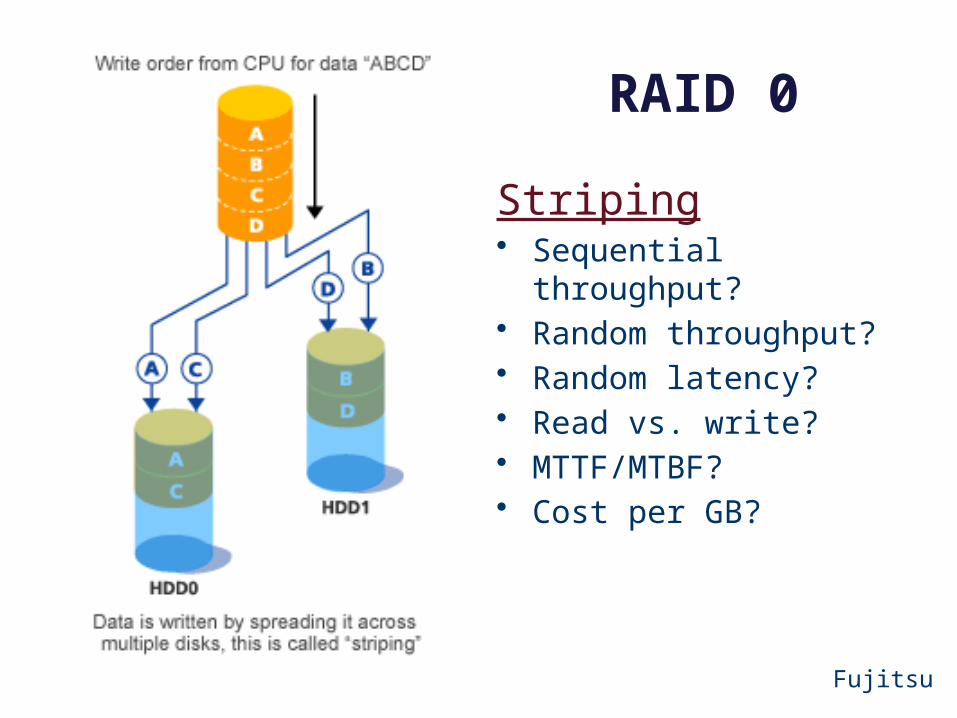
RAID 0
Fujitsu
Striping• Sequential throughput?• Random throughput?• Random latency?• Read vs. write?• MTTF/MTBF?• Cost per GB?
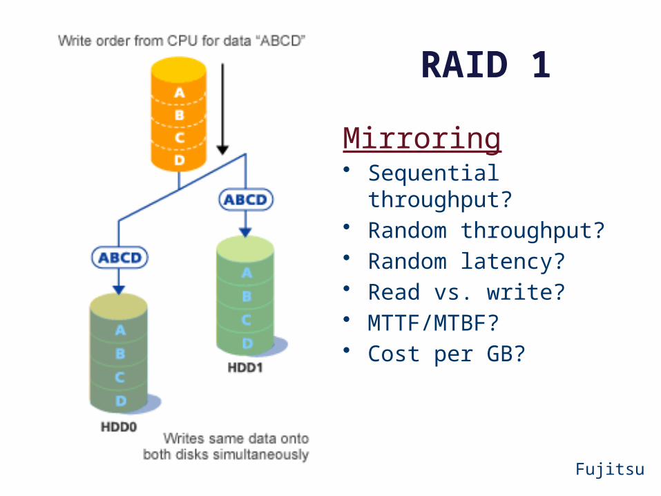
RAID 1
Fujitsu
Mirroring• Sequential throughput?• Random throughput?• Random latency?• Read vs. write?• MTTF/MTBF?• Cost per GB?
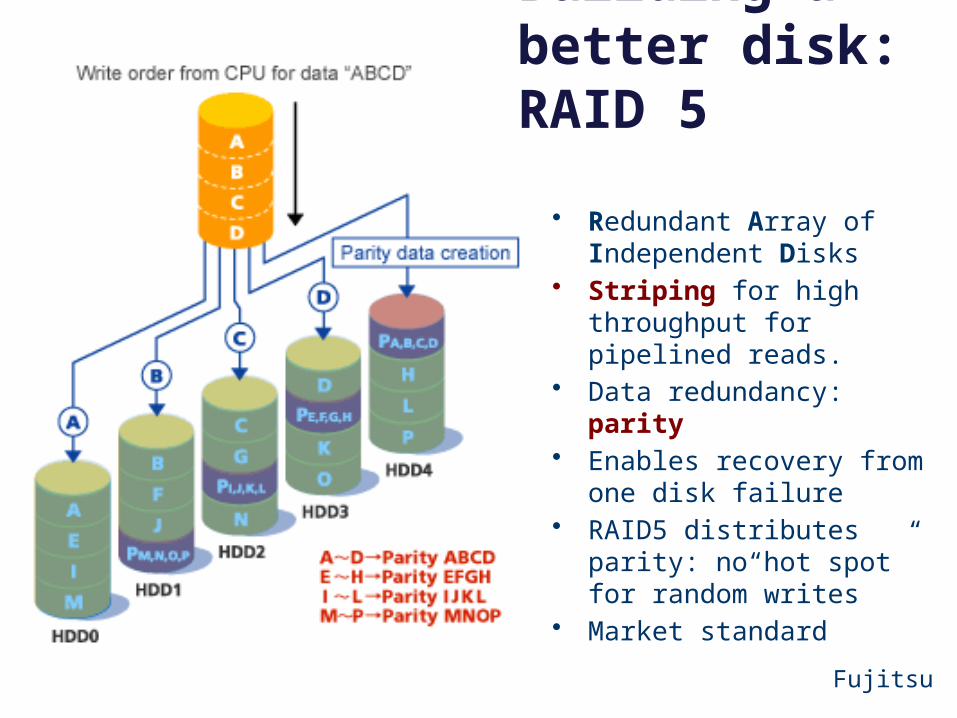
Fujitsu
• Redundant Array of Independent Disks
• Striping for high throughput for pipelined reads.
• Data redundancy: parity• Enables recovery from one
disk failure• RAID5 distributes parity:
no“hot spot” for random writes
• Market standard
Building a better disk: RAID 5
The remaining slides were not covered in class.They deal with the response time curve and why always “bends up”. They are not to be tested.
[graphic from IBM.com]
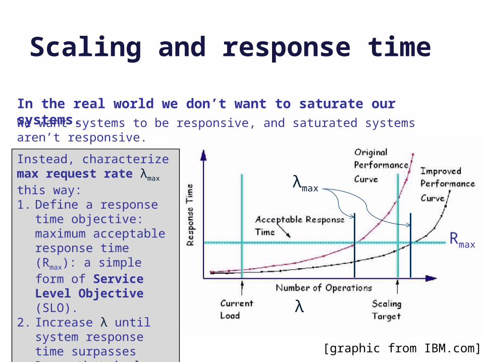
Scaling and response time
In the real world we don’t want to saturate our systems.
We want systems to be responsive, and saturated systems aren’t responsive.
Instead, characterize max request rate λmax this way:1. Define a response time
objective: maximum acceptable response time (Rmax): a simple form of Service Level Objective (SLO).
2. Increase λ until system response time surpasses Rmax : that is λmax. λ
Rmax
λmax
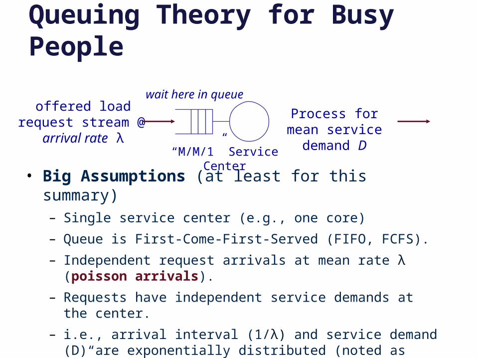
Queuing Theory for Busy People
• Big Assumptions (at least for this summary)– Single service center (e.g., one core)
– Queue is First-Come-First-Served (FIFO, FCFS).
– Independent request arrivals at mean rate λ (poisson arrivals).
– Requests have independent service demands at the center.
– i.e., arrival interval (1/λ) and service demand (D) are exponentially distributed (noted as “M”) around some mean.
– These assumptions are rarely true for real systems, but they give a good “back of napkin” understanding of queue behavior.
“M/M/1” Service Center
offered loadrequest stream @
arrival rate λ
wait here in queue
Process for mean service demand D
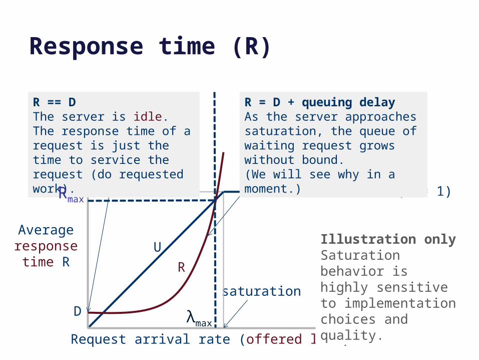
Response time (R)
Request arrival rate (offered load)
Average response
time R
saturation
Illustration onlySaturation behavior is highly sensitive to implementation choices and quality.
saturation (U = 1)
U
R
D
R == DThe server is idle. The response time of a request is just the time to service the request (do requested work).
R = D + queuing delayAs the server approaches saturation, the queue of waiting request grows without bound.(We will see why in a moment.)
Rmax
λmax
(Max request load)
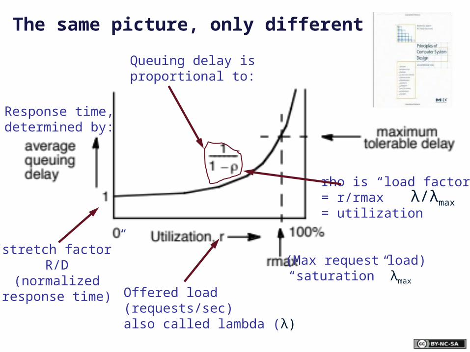
Offered load(requests/sec)also called lambda (λ)
“saturation” λmax
Response time,determined by:
Queuing delay is proportional to:
rho is “load factor”= r/rmax= utilization
“stretch factor”R/D
(normalizedresponse time)
The same picture, only different
λ/λmax
Little’s Law
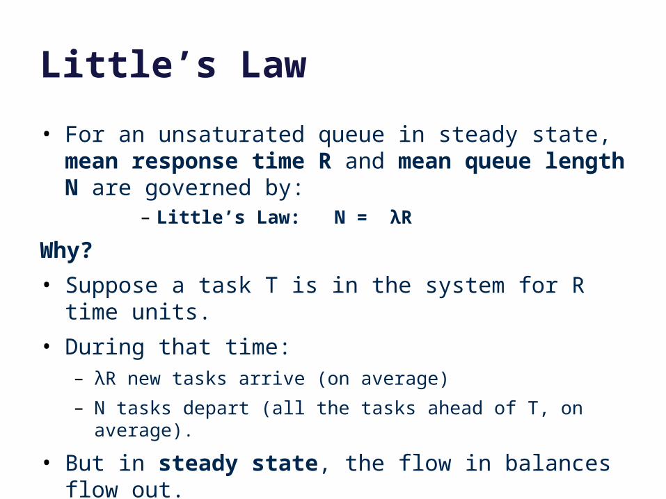
• For an unsaturated queue in steady state, mean response time R and mean queue length N are governed by:
– Little’s Law: N = λR
Why?
• Suppose a task T is in the system for R time units.
• During that time:– λR new tasks arrive (on average)
– N tasks depart (all the tasks ahead of T, on average).
• But in steady state, the flow in balances flow out.– Note: this means that throughput X = λ in steady state.
Inverse Idle Time “Law”
R
1(100%)U
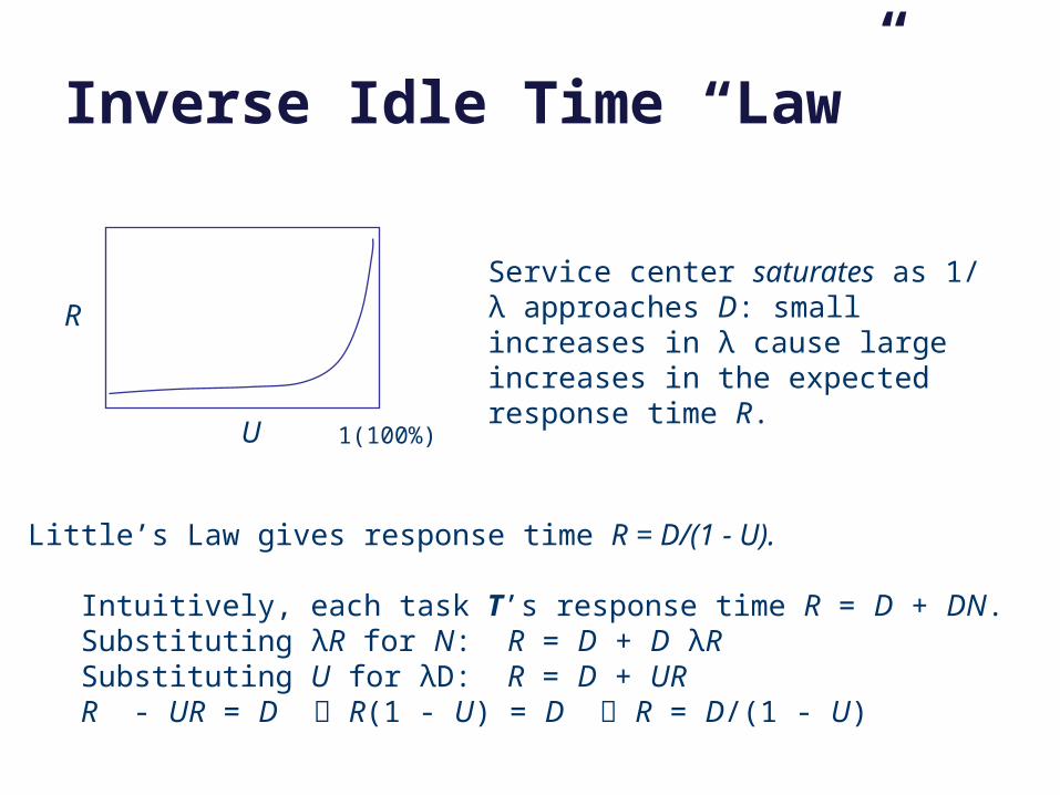
Little’s Law gives response time R = D/(1 - U).
Intuitively, each task T’s response time R = D + DN.Substituting λR for N: R = D + D λR Substituting U for λD: R = D + URR - UR = D R(1 - U) = D R = D/(1 - U)
Service center saturates as 1/ λ approaches D: small increases in λ cause large increases in the expected response time R.
Why Little’s Law is important
1. Intuitive understanding of FCFS queue behavior.
Compute response time from demand parameters (λ, D).
Compute N: how much storage is needed for the queue.
2. Notion of a saturated service center.
Response times rise rapidly with load and are unbounded.
At 50% utilization, a 10% increase in load increases R by 10%.
At 90% utilization, a 10% increase in load increases R by 10x.
3. Basis for predicting performance of queuing networks.
Cheap and easy “back of napkin” estimates of system performance based on observed behavior and proposed changes, e.g., capacity planning, “what if” questions.
Guides intuition even in scenarios where the assumptions of the theory are not met.

Utilization: cartoon version
saturated
Request arrival rate (offered load)
Utilization(also called load factor)
saturation
peak rate
U = XDX = throughputD = service demand, i.e., how much time/work to complete each request.
U = 1 = 100%The server is saturated. It has no spare capacity. It is busy all the time.
This graph shows utilization (e.g., of a server) as a function of offered load. It is idealized: each request works for D time units on a single service center (e.g., a single CPU core).
1 == 100%
Utilization
• What is the probability that the center is busy?– Answer: some number between 0 and 1.
• What percentage of the time is the center busy?– Answer: some number between 0 and 100
• These are interchangeable: called utilization U
• The probability that the service center is idle is 1-U.
The Utilization Law
• If the center is not saturated then:– U = λD = (arrivals/T) * service demand
• Reminder: that’s a rough average estimate for a mix of independent request arrivals with average service demand D.
• If you actually measure utilization at the device, it may vary from this estimate.– But not by much.


![Bitcoin Jeff Chase Duke University. Some sources [NBFMG15]](https://img.pdfslide.net/doc/110x75/5697bfc61a28abf838ca74a0/bitcoin-jeff-chase-duke-university-some-sources-nbfmg15.jpg)