Chapter 7Filter Design Techniques

2018/9/18 DSP 2

Introduction

Filter – An important class of LTI systems

We discuss frequency-selective filters mostly: LP, HP, …

Three stages in filter design:

Specification: application dependent

“Design”: approximate the given spec. using a causal discrete-time system

Realization: architectures and circuits (IC) implementation

IIR filter design techniques

FIR filter design techniques

2018/9/18 DSP 3

2018/9/18 DSP 4

The overall system behaves as a linear time-invariant continuous-time system with frequency response

It is straightforward to convert from specifications on the effective continuous-time filter to specifications on the discrete-time filter.

( ), | |< /T( )

0, | |> /T

j T

eff

H eH j

( ) ( ), | |<j

effH e H jT

2018/9/18 DSP 5

Example 7.1 : Determining Specifications for a Discrete-Time Filter

If a discrete-time filter will be used as a lowpass filter, we want the overall system have the following specifications when the sampling rate is 104 samples/s (T = 10–4 s): The gain should be within 0.01 of unity in the

frequency band 0 2(2000)

The gain should be no greater than 0.001 in the frequency band 2(3000) .

For this specific example, the parameter would be:

d1 = 0.01 ( 20log10(1+ d1)=0.086dB ),

d2 = 0.001 ( 20log10d2=-60dB ),

p = 2(2000),

s = 2(3000).

Since the sampling rate is 104 samples/s, the gain of the ideal system is identically zero above 2(5000) due to the ideal discrete-to-continuous (D/C) converter.

( )effH j

2018/9/18 DSP 6

2018/9/18 DSP 7

7.1 Design of Discrete-Time IIR Filters from Continuous-Time Filters The art of continuous-time IIR filter design is

highly advanced and, since useful results can be achieved, it is advantageous to use the design procedures already developed for continuous-time filters

Many useful continuous-time IIR design methods have relatively simple closed-form design formula

The standard approximation methods that work well for continuous-time IIR filters do not lead to simple closed-form design formula when these methods are applied directly to the discrete-time IIR case.

2018/9/18 DSP 8

Why based on continuous-time IIR filters?

Continuous-time IIR filter design methods have been well developed.

Continuous-time IIR filters often have simple closed-from design formulas.

Direct Discrete-time IIR filter design methods often don’t have closed-form formulas.

There are two types of transformations Transformation from continuous-time to discrete-

time

Transformation from one type filter to another type (so called frequency transformation)

2018/9/18 DSP 9

Objective: To find H(z)

Design Concept:

(1)Analog Filter H(s): Butterworth, Chebyshev,..

Already developed, procedure is fixed

(2) Transformation:

H(s)H(z)

2018/9/18 DSP 10

Appendix B: Continuous-time Filter

2018/9/18 DSP 11

2018/9/18 DSP 12

2018/9/18 DSP 13

2018/9/18 DSP 14

2018/9/18 DSP 15

2018/9/18 DSP 16

2018/9/18 DSP 17

2018/9/18 DSP 18

2018/9/18 DSP 19

2018/9/18 DSP 20

2018/9/18 DSP 21

2018/9/18 DSP 22

2018/9/18 DSP 23

2018/9/18 DSP 24

2018/9/18 DSP 25

Filter Design by Impulse Invariance

In the impulse invariance design procedure for transforming continuous-time filters into discrete-time, the impulse response of the discrete-time filter is chosen as equally spaced samples of the impulse response of the continuous-time filter :

where Td represents a sampling interval.

It follows that the frequency response of the discrete-time filter obtained through Eq. (7.4) is related to the frequency response of the continuous-time filter by

[ ] ( ),d c dh n T h nT

2( ) ( ).j

c

k d d

H e H j j kT T

2018/9/18 DSP 26

If the continuous-time filter is bandlimited, so that

then

I.e., the discrete-time and continuous-time frequency responses are related by a linear scaling of the frequency axis, namely,

( ) 0, / ,c dH j T

( ) ( ), | | ;j

c

d

H e H jT

for .dT

2018/9/18 DSP 27

2018/9/18 DSP 28

2018/9/18 DSP 29

Comparison Poles of Hc(s): s=sk, k=1,2,…, N (s-plane)

Poles of H(z):

Coefficients of Hc(s): Ak

Coefficients of H(z): TdAk

Hc(s) is stable the real part of sk is less than zero.

the magnitude of is less than unity

the corresponding poles is inside the unit circle

H(z) is stable

, 1,2,..., ( )k ds T

kz e k N z plane

k ds Te

30

Filter Design by Impulse Invariance

(MATLAB function: impinvar)

)(sHc spsp AR and ,,,

}{ ks4. Transform analog poles

1. Choose Td and determine the analog frequencies

2. Design an analog filter using specifications

3. Partial fraction expansion

into digital poles

to obtain transfer function

Td

p

p

Td

ss

dkTse

N

1k k

kc

ss

AsH

0t0

0teAth

N

1k

ts

kc

k

•Corresponding impulse response

N

1k1Ts

kd

ze1

ATzH

dk

31

Example

Find the discrete equivalent system of the following

transfer function:

2018/9/18 DSP 32

Example 7.2 : Impulse Invariance with a Butterworth Filter.

By applying impulse invariance to an appropriate Butterworth continuous-time filter. The specifications for the discrete-time filter are

0.89125 |H(ej)| 1, 0 || 0.2,

|H(ej)| 0.17783, 0.3 || .

Since the parameter Td cancels in the impulse invariance procedure, we can choose Td = 1, so that = . Hence,

0.89125 |Hc(j)| 1, 0 || 0.2,

|Hc(j)| 0.17783, 0.3 || .

Since the magnitude response of an analog Butterworth filter is monotonic function of frequency, the above specifications will be satisfied if

|Hc(j0.2)| 0.89125 and |Hc(j0.3)| 0.17783.

Then,

So, N = 5.8858 and c = 0.70474.

2 22 20.2 1 0.3 1

1 and 10.89125 0.17783

N N

c c

2018/9/18 DSP 33

However, N must be rounded up to the next highest integer:

N = 6 and new value of c = 0.7032.

It means that there are 12 poles of the magnitude-squared function

are uniformly distributed in angle on a circle of radius c = 0.7032.

The poles of HC(s) are the three pole pairs in the left half of the s-plane with the following coordinates:

Pole pair #1 : -0.182 j(0.679),

Pole pair #2: -0.497 j(0.497),

Pole pair #3: -0.679 j(0.182).

Therefore,

2( ) ( ) 1/ 1 ( / ) N

c c cH s H s s j

2 2 2

0.12093( )

( 0.3640 0.4945)( 0.9945 0.4945)( 1.3585 0.4945)cH s

s s s s s s

2018/9/18 DSP 34

2018/9/18 DSP 35

Express Hc(s) as a partial fraction expansion, perform the transformation, and combine complex-conjugate terms, the resulting system function of the digital filter is:

1 1

1 2 1 2

1

1 2

0.2871 0.4466 2.1428 1.1455( )

1 1.2971 0.6949 1 1.0691 0.3699

1.8557 0.6303

1 .09972 0.2570

z zH z

z z z z

z

z z

2018/9/18 DSP 36

Bilinear Transformation : avoid the problem of aliasing

An algebraic transformation between the variables and that maps the entire

-axis in the -plane to one revolution of the unit circle in the -plane.

s z

j s z

0

'

0

0

'

( 1)

' '

0

1 0

0

nonlinear

( ) ( ) ( )

Let , ( 1)

( ) ( ) (( 1) )

( ) (( 1) ) (( 1) )2

( )First order ( )

( )

t

c c ct

nT

c c cn T

c c c

cc

c

y t y t dt y t

t nT t n T

y nT y t dt y n T

Ty nT y n T y n T

d Y sH s

c s c X s

d X

1 0

0 1 0

'

0 1 0

( ) ( ) ( )

( ) ( ) ( )

( ) ( ) ( )

c c c

cc c

c c c

s c sY s c Y s

dy td x t c c y t

dt

d x nT c y nT c y nT

'(( 1) )cy n T

'( )cy nT

2018/9/18 DSP 37

' 0 0

1 1

0 0 0 0

1 1 1 1

0 0

1 1

1 10 0

1 1

( ) ( ) ( )

( ) ( ) ( ) (( 1) ) (( 1) ) (( 1) )2

[ ] [ 1] [ ] [ 1] [ ] [ 1]2

( )(1 ) ( )(1 ) ( )(2

c c c

c c c c c c

c dy nT y nT x nT

c c

c d c dTy nT y nT x nT y n T x n T y n T

c c c c

c dTy n y n y n y n x n x n

c c

c dTY z z Y z z X z

c c

1

1

1

10

01

11 10

1 011

2 (1 )

(1 )

1 )

(1 )2( )

( )2 (1 )( )

1 (1 )2 (1 )

( ) ( )| zcs

T z

z

d Tz

dcY zH z

cT zX zz z c c

c T z

H z H s

2018/9/18 DSP 38

Bilinear Transformation

With Hc(s) denoting the continuous-time system function and H(z) the discrete-time system function, the bilinear transformation corresponds to replacing s by

that is,

To develop the properties of the algebraic transformation specified in Eq. (7.20), we solve for z to obtain

and, substituting into Eq. (7.22), we obtain

1

1

2 1;

1d

zs

T z

s j

1

1

2 1( ) .

1c

d

zH z H

T z

1 ( / 2),

1 ( / 2)

d

d

T sz

T s

1 / 2 / 2.

1 / 2 / 2

d d

d d

T j Tz

T j T

2018/9/18 DSP 39

Next, to show that the -axis of the s-plane maps onto the unit circle, we substitute into Eq. (7.22), obtaining

From Eq. (7.24), it is clear that |z| = 1 for all values of s on the

-axis. That is, the -axis maps onto the unit circle, so Eq. (7.24) takes the form

To derive a relationship between the variables and , it is useful to return to Eq. (7.20) and substitute . We obtain

1 / 2.

1 / 2

d

d

j Tz

j T

j

2 1,

1

j

j

d

es

T e

s j

j j

1 / 2.

1 / 2

j d

d

j Te

j T

jz e

2018/9/18 DSP 40

or, equivalently,

Equating real and imaginary parts on both sides of Eq. (7.27) leads to the relations and

or

/ 2

/ 2

2 2 ( sin / 2) 2tan( / 2).

2 (cos / 2)

j

j

d d

e j js j

T e T

2arctan( / 2).dT

0 2

tan( / 2),dT

Filter Design by the bilinear transformation

(MATLAB function: bilinear)

1

1

d z1

z1

T

2s

1

1

d

cz1

z1

T

2HzH

•Td cancels out so we can ignore it

•We can solve the transformation for z as

2/Tj2/T1

2/Tj2/T1

s2/T1

s2/T1z

dd

dd

d

d

js

1. Choose T and determine

the analog frequencies)

2tan(

2 p

pT

)

2tan(

2 ss

T

spsp AR and ,,,2. Design an analog filter using specifications

3. Bilinear transformation

)(sH c

2018/9/18 DSP 42

2018/9/18 DSP 43

2018/9/18 DSP 44

2018/9/18 DSP 45

Bilinear Transformation Algorithm

Step 1: define specifications of filter Ripple in frequency bands Critical frequencies: passband edge, stopband edge, and/or cutoff

frequencies. Filter band type: lowpass, highpass, bandpass, bandstop.

Step 2: select filter structure type and its order: Bessel, Butterworth, Chebyshev type I, Chebyshev type II or inverse Chebyshev, elliptic.

Step 3: critical frequencies prewarping: = [2/Td]tan(/2)

Step 4: bilinear transform by replacing s variable in H(s) bys = [2/Td][(1-z-1)/(1+z-1)]

to obtain H(z). Step 5: verify the result. If it does not meet requirement, return

to step 2.

2018/9/18 DSP 46

Discussion

Avoid the problem of aliasing

Nonlinear compression of the frequency axis Frequency distortion

Phase:

1

1

2 1 2 1( ) ( )1 1

2 : tan( ) ---Nonlinear

2

|j

j

d d

d

jz e

z es

T z T e

Phase angleT

2018/9/18 DSP 47

Example : Bilinear transformation of a Butterworth filter

Consider the discrete-time filter specifications of Example 7.2, in which we illustrated the impulse invariance technique for the design of a discrete-time filter. The specifications on the discrete-time filter are

0.89125 |H(ej)| 1, 0 0.2,

|H(ej)| 0.17783, 0.3 .

The critical frequencies of the discrete-time filter must be prewarped to the corresponding continuous-time frequencies using the relationship:

= [2/Td]tan(/2)

given Td = 1: 0.89125 |Hc(j )| 1, 0 2/Td tan(0.2/2),

|Hc(j )| 0.17783, 2/Td tan(0.3/2) .

Since a continuous-time Butterworth filter has a monotonic magnitude response, so

|Hc(j2tan(0.1)| 0.89125 and |Hc(j2tan(0.15))| 0.17783.

The form of the magnitude-squared function for the Butterworth filter is

|Hc(j)|2 = 1/[1 + (/c)2N] .

2018/9/18 DSP 48

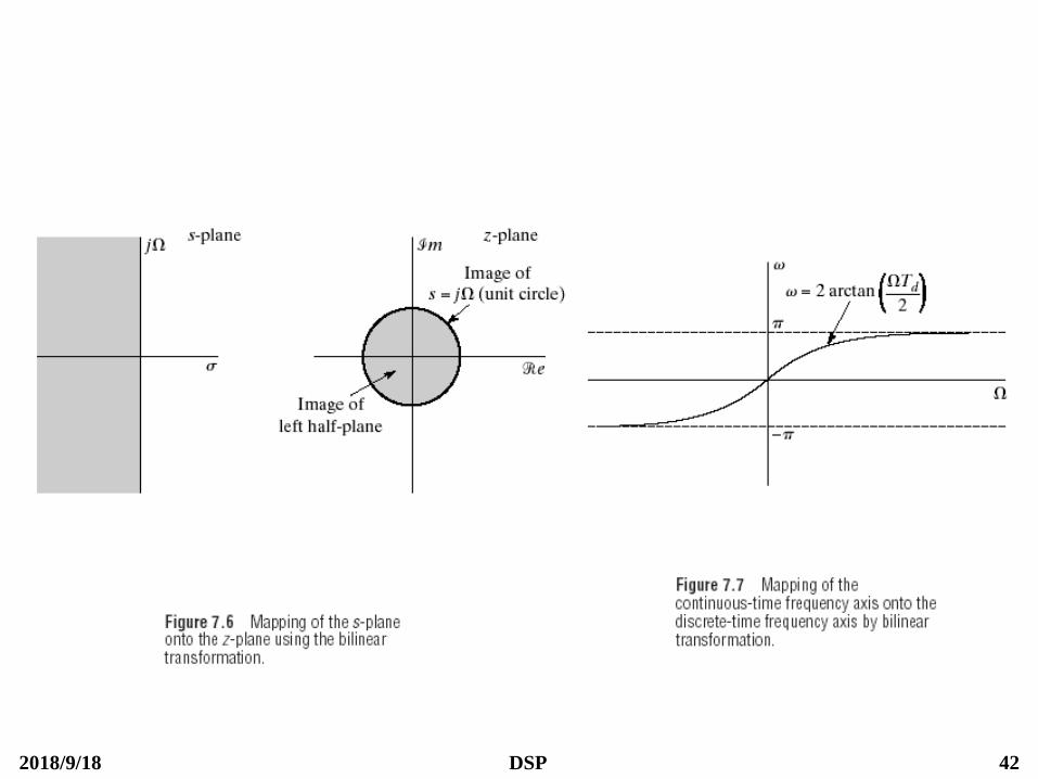
Solving for N and c, we obtain

1+(2tan(0.1)/c)2N = (1/0.89)2

and 1+(2tan(0.15)/c)2N = (1/0.178)2 .

N = 5.305

Since N must be an integer, we choose N = 6. Thus, we obtain c = 0.766.

In the s-plane, the 12 poles of the magnitude-squared function are uniformly distributed in angle on a circle of radius 0.766. The system function of the continuous-time filter obtained by selecting the left half-plane poles is:

The system function for the discrete-time filter is then obtained by applying the bilinear transformation with Td = 1. The result is

2 2 2

0.20238( ) .

( 0.3996 0.5871)( 1.0836 0.5871)( 1.4802 0.5871)cH s

s s s s s s

1 6

1 2 1 2

1 2

0.0007378(1 )( )

(1 1.2686 0.7051 )(1 1.0106 0.3583 )

1 .

(1 0.9044 0.2155 )

zH z

z z z z

z z

2018/9/18 DSP 49

2018/9/18 DSP 50

The general Nth-order Butterworth discrete-time filter has magnitude-squared function

where

2

2

1( ) ,

tan( / 2)1

tan( / 2)

j

N

c

H e

tan( / 2) / 2.c c dT

2018/9/18 DSP 51

Example : Butterworth Approximation

2018/9/18 DSP 52

Example : Chebyshev Approximation

2018/9/18 DSP 53

2018/9/18 DSP 54

Example : Elliptic Approximation

2018/9/18 DSP 55

Frequency Transformation

2018/9/18 DSP 56

Frequency Transformation

2018/9/18 DSP 57

Frequency Transformation

2018/9/18 DSP 58

Frequency Transformation

2018/9/18 DSP 59

Frequency Transformation

2018/9/18 DSP 60

Frequency Transformation

2018/9/18 DSP 61

DESIGN OF FIR FILTERS BY WINDOWING

FIR filter are almost entirely restricted to discrete-time implementations.

The design techniques for FIR filters are based on directly approximating the desired frequency response of the discrete-time system.

Most techniques for approximating the magnitude response of an FIR system assume a linear phase constraint, thereby avoiding the problem of spectrum factorization that complicates the direct design of IIR filters.

The windowing technique is the simplest method of FIR filter design.

This method generally begins with an ideal desired frequency response, Hd(ej), and evaluates its corresponding impulse response, hd[n]. Then, the desired impulse response, h[n], will be obtained by truncating hd[n]. with selected window function, w[n].

2018/9/18 DSP 62

The simplest method of FIR filter design is called the window method. This method generally begins with an ideal desired frequency response that can be represented as

Where is the corresponding impulse response sequence, which can be expressed in terms of as

The simplest way to obtain a causal FIR filter from is to define a new system with impulse response h[n] given by

More generally, we can represent h[n] as the product of the desired impulse response and a finite-duration “window” w[n]; i.e.,

dh n( )j

dH e

dh n

( ) [ ] ,j j n

d d

n

H e h n e

1[ ] ( ) .

2

j j n

d dh n H e e d

[ ], 0 ,[ ]

0, otherwise.

dh n n Mh n

[ ] [ ] [ ],dh n h n w n

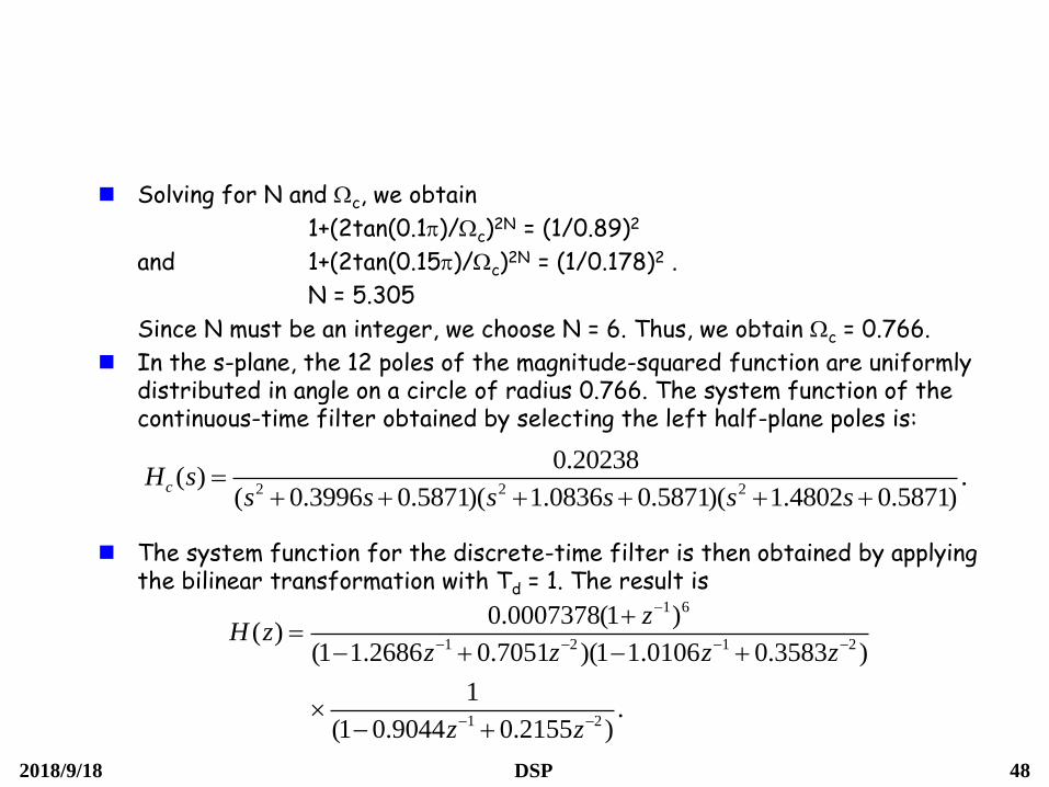
2018/9/18 DSP 63

Where, for simple truncation as in Eq. (7.42), the window is the rectangular window

It follows from the modulation, or windowing, theorem (Section 2.9.7) that

Where

( )1( ) ( ) ( ) .

2

j j j

dH e H e W e d

1, 0 ,[ ]

0, otherwise.

n Mw n

( 1)/ 2

0

1 sin[ ( 1) / 2]( ) .

1 sin( / 2)

j MMj j n j M

jn

e MW e e e

e

2018/9/18 DSP 64

Convolution process implied by truncation of the ideal impulse response

Typical approximation resulting from windowing the ideal impulse response

2018/9/18 DSP 65

2018/9/18 DSP 66

Properties of Commonly Used Windows

Window Type Time-Domain Sequence

Rectangular

Bartlett(triangular)

Hanning

Hamming

Blackman

1, 0 ,[ ]

0, otherwise

n Mw n

2 / , 0 / 2,

[ ] 2 2 / , / 2 ,

0, otherwise

n M n M

w n n M M n M

0.5 0.5cos(2 / ), 0 ,[ ]

0, otherwise

n M n Mw n

0.54 0.46cos(2 / ), 0 ,

[ ]0, otherwise

n M n Mw n

0.42 0.5cos(2 / ) 0.08cos(4 / ), 0 ,[ ]

0, otherwise

n M n M n Mw n

2018/9/18 DSP 67

2018/9/18 DSP 68

2018/9/18 DSP 69

2018/9/18 DSP 70

2018/9/18 DSP 71

Note that all the windows have the property that

i.e., they are symmetric about the point M/2. As a result, their Fourier transforms are of the form

where is a real, even function of

Consider the frequency-domain representation. Suppose

Then

where is real and even.

/ 2( ) ( ) ,j j j M

eW e W e e

[ ], 0 ,[ ]

0, otherwise;

w M n n Mw n

/ 2( ) ( ) ,j j j M

d eH e H e e

Incorporation of Generalized Linear Phase

( )j

eW e .

[ ] [ ]d dh M n h n

( )j

eH e

2018/9/18 DSP 72

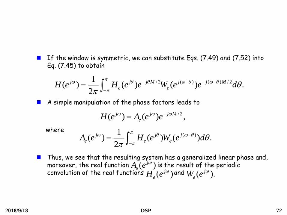
If the window is symmetric, we can substitute Eqs. (7.49) and (7.52) into Eq. (7.45) to obtain

A simple manipulation of the phase factors leads to

where

Thus, we see that the resulting system has a generalized linear phase and, moreover, the real function is the result of the periodic convolution of the real functions and

/ 2( ) ( ) ,j j j M

eH e A e e

/ 2 ( ) ( ) / 21( ) ( ) ( ) .

2

j j j M j j M

e eH e H e e W e e d

( )1( ) ( ) ( ) .

2

j j j

e e eA e H e W e d

( )j

eA e

( ).j

eW e ( )j

eH e

2018/9/18 DSP 73

The desired frequency response is defined as

Where the generalized linear phase factor has been incorporated into the definition of the ideal lowpass filter. The corresponding ideal impulse response is

For . It is easily shown that , so if we use a symmetric window in the equation

then a linear-phase system will result.

/ 2

c

, ,[ ]

0, ,

j M

cj

lp

eH e

Example : Linear-Phase Lowpass Filter

n [ ] [ ]lp lph M n h n

/ 2 sin[ ( / 2)]1[ ]

2 ( / 2)

c

c

j M j n clp

n Mh n e e d

n M

sin[ ( / 2)][ ] [ ],

( / 2)

c n Mh n w n

n M

2018/9/18 DSP 74

2018/9/18 DSP 75

2018/9/18 DSP 76

The tradeoff between the mainlobe width and sidelobe area can be quantified by seeking the window function that is maximally concentrated around =0 in the frequency domain.

The Kaiser window, a near-optimal window, is defined as

α=M/2, I0(.): the zeroth-order modified Bessel function of the first kind.

The transition region has width

for the lowpass filter approximation. Defining

2 1/ 2

0

0

[ (1 [( ) / ] ) ], 0 n M,

[ ]

0, otherwise,

I n

w n I

s p

1020log ,A d

The Kaiser Window Filter Design Method

2018/9/18 DSP 77

Kaiser determined empirically that the value of needed to achieve a specified value of A is given by

( Recall that the case is the rectangular window for which A = 21 ) Furthermore, Kaiser found that to achieve prescribed values of A and , M must satisfy

0.4

0.1102( 8.7), 50,

0.5842( 21) 0.07886( 21), 21 50,

0.0, 21.

A A

A A A

A

8.

2.285

AM

0

2018/9/18 DSP 78

2018/9/18 DSP 79

Example : Kaiser Window Design of a Lowpass Filter

Consider the lowpass digital filter specifications:

0.99 |H(ej)| 1.01, || 0.4,

|H(ej)| 0.001, 0.6 || .

Using the design formulas for the Kaiser window to design an FIR lowpass filter to meet prescribed specifications.

First, we set d = 0.001.

Next, the cutoff frequency of the ideal lowpass filter is

c = (p + s)/2 = 0.5 .

To determine the parameters of the Kaiser window, we first compute

= s – p = 0.2, A = -20log10d = 60.

Then, = 5.653, M = 37.

The impulse response of the filter is:

where = M/2 = 18.5

2 1/ 2

0

0

sin ( ) [ (1 [( ) / ] ) ], 0 n M,

[ ] ( )

0, otherwise,

c n I n

w n n I

2018/9/18 DSP 80

2018/9/18 DSP 81

Highpass FilterThe ideal highpass filter with generalized linear phase has the frequency response

The corresponding impulse response can be found by evaluating the inverse transform of , or we can observe that

where is given by Eq. (7.56). Thus is

c

/ 2

c

0, < ,( )

, .

j

hp j MH e

e

/ 2( ) ( ),j j M j

hp lpH e e H e

( )j

hpH e

7.3 EXAMPLES OF FIR FILTER DESIGN BY THE KAISER WINDOW METHOD

( )j

lpH e [ ]hph n

sin ( / 2)sin ( / 2)[ ] ,

( / 2) ( / 2)

chp

n Mn Mh n n

n M n M

2018/9/18 DSP 82

Suppose that we wish to design a filter to meet the highpass specifications

where

2

1 1

( ) ,

1 ( ) 1 ,

j

s

j

p

H e

H e

d

d d

Example : Kaiser Window Design of a Highpass Filter

1 20.35 , 0.5 , 0.021.s p d d d

2018/9/18 DSP 83

This is a Type I filter (M=24).

Approximation error

= 0.0213 > 0.021!!

Increase M to 25 Not good! Why?

Since the error is less than 0.021

everywhere except at the stopband edge

2018/9/18 DSP 84

This is a Type II filter (M=25): a zero at –1.

, =

Increase the order by one worse result

Increase M to 26 type I that exceeds

the specification

Type II FIR are not appropriate

approximations for either highpass

or bandstop filters

2018/9/18 DSP 85

The previous discussion of highpass filter design can be generalized to the case of multiple passbands and stopbands. Figure 7.28 shows an ideal multiband frequency selective frequency response.

If such a magnitude function is multiplied by a linear phase factor , the corresponding ideal impulse response is

where is the number of bands and

1

1

sin ( / 2)[ ] ( ) ,

( / 2)

mbN

kmb k k

k

n Mh n G G

n M

/ 2j Me

1 0.mbNG

mbN

2018/9/18 DSP 86

If hmb[n] is multiplied by a

Kaiser window, the type

of approximations will occur

at each of the discontinuities.

The Kaiser’s formulas for

the window parameters can

be applied to this case to

predict approximation errors

and transition widths.

2018/9/18 DSP 87

For an ideal discrete-time differentiator with a linear phase, the appropriate frequency response is

( We have omitted the factor 1/T. ) The corresponding ideal impulse response is

If is multiplied by a symmetric window of length ( M + 1 ), then it is easily shown that h[n] = -h[M-n]. Thus, the resulting system is either a type III or a type IV generalized linear-phase system

/ 2( ) ( ) , - < < .j j M

diffH e j e

7.3.2 Discrete-Time Differentiators

cos ( / 2) sin ( / 2)[ ] , - <n< .

( / 2) ( / 2)diff

n M n Mh n

n M n M

[ ]diffh n

2018/9/18 DSP 88

To illustrate the window design of a differentiator, suppose M = 10 and = 2.4. The resulting response characteristics are shown if Figure 7.29.

Figure 7.29(a) shows the antisymmetric impulse response. Since M is even, the system is a type III linear-phase system, which implies that H(z) has zeros at both z = +1(w =

0) and z = -1(w = ). This is clearly displayed in the magnitude response shown in Figure 7.29(b).

The phase is exact linear, since type III systems have a /2

radian constant phase shift plus a linear phase corresponding in this case to M/2 = 5 samples delay. Figure 7.29(c) shows the amplitude approximation error

where is the amplitude of the approximation.

Example : Kaiser Window Design of a Differentiator

0( ) ( ), 0 0.8j

diffE A e

0 ( )jA e

2018/9/18 DSP 89

2018/9/18 DSP 90

Example : Kaiser Window Design of a Differentiator

Type IV linear-phase systems do not constrain H(z) to have a zero at z=-1.

This type of system leads to much better approximation to the amplitude function, as shown in Figure 7.30, for M = 5 and = 2.4.

In this case, the amplitude approximation error is very small up to and beyond w= 0.8

2018/9/18 DSP 91

2018/9/18 DSP 92

Case 1: M=10, β=2.4 Type III Zeros

at 0 and –1. Approximation is not good at ω =π.

Case 2: M=5, β=2.4 Type IV

Zeros at 0. Approximation error is smaller.

2018/9/18 DSP 93

Advantages and Disadvantages of the Window Method

Simplicity It is simple to apply and simple to understand. It involves a minimum

amount of computational effort, even for the more complicated Kaiser window.

Lack of flexibility Both the peak passband and stopband ripples are approximately equal, so

that the designer may end up with either too small a passband ripple or too large a stopband attenuation.

Unprecision Because of the effect of convolution of the spectrum of the window

function and the desired response, the passband and stopband edge frequencies cannot be precisely specified.

Clumsy (trial and error technique) For a given window (except the Kaiser) the maximum ripple amplitude in the

filter response is fixed regardless of how large we make N. Thus the stopband attenuation for a given window is fixed. Thus, for a given attenuation specification, the filter designer must find a suitable window.

Lack of capability In some applications, the expression for the desired filter response, Hd(),

will be too complicated for hd[n] to be obtained analytically. In these cases hd[n] may be obtained via the frequency sampling method before the window function is applied.

2018/9/18 DSP 94

OPTIMUM APPROXIMATIONS OF FIR FILTERS

We wish to design a filter that is the “best” that can be achieved for a given value of M.

Why computer-aided design?

-- Optimum: minimize an error criterion

-- More freedom in selecting constraints.

(In windowing method: must )

2018/9/18 DSP 95

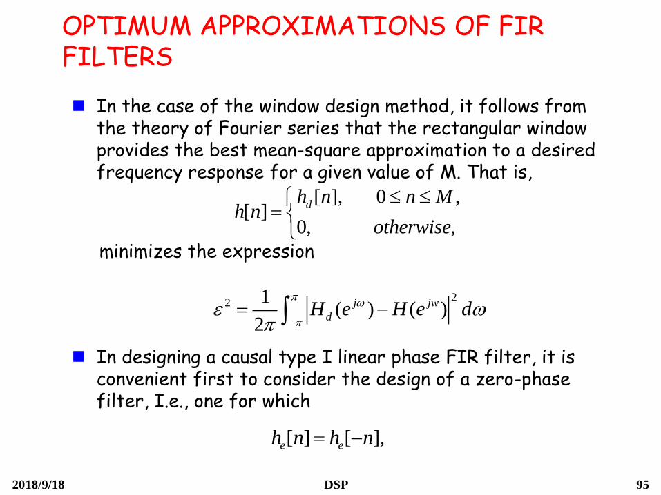
OPTIMUM APPROXIMATIONS OF FIR FILTERS

In the case of the window design method, it follows from the theory of Fourier series that the rectangular window provides the best mean-square approximation to a desired frequency response for a given value of M. That is,

minimizes the expression

In designing a causal type I linear phase FIR filter, it is convenient first to consider the design of a zero-phase filter, I.e., one for which

[ ], 0 ,[ ]

0, ,

dh n n Mh n

otherwise

22 1

( ) ( )2

j jw

dH e H e d

[ ] [ ],e eh n h n

2018/9/18 DSP 96

And then to insert sufficient delay to make it causal. Consequently, we consider satisfying the condition of Eq. (7.74). The corresponding frequency response is given by

with L=M/2 an integer or, because of Eq. (7.74)

(7.76)

Note that is real, even, and periodic function of . A causal system can be obtained from by delaying it by L = M / 2 samples. The resulting system has impulse response

and frequency response

( ) [ ] ,L

j j n

e e

n L

A e h n e

[ ]eh n

1

( ) [0] 2 [ ]cos( ).L

j

e e e

n

A e h h n n

( )j

eA e

[ ]eh n

[ ] [ / 2] [ ]eh n h n M h M n

/ 2( ) ( ) .j j j M

eH e A e e

2018/9/18 DSP 97

2018/9/18 DSP 98

The Parks-McClellan algorithm is based on reformulating the filter design problem as a problem in polynomial approximation. Specifically, the terms cosn) in Eq. (7.76) can be expressed as a sum of powers of cos in the form

Where is an nth-order polynomial. Consequently, Eq. (7.76) can be rewritten as an Lth-order polynomial in cos . Specifically,

Where the are constants that are related to , the values of the impulse response. With the substitution

, we can express Eq. (7.80) as

where P(x) is the Lth-order polynomial

cos '( ) ( ) |j

e xA e P x

0

( ) (cos ) , (7.80)L

j k

e k

k

A e a

cos( ) (cos ),nn T ( )nT x

'ka s [ ]eh n

cosx

0

( ) .L

k

k

k

P x a x

2018/9/18 DSP 99

To formalize the approximation problem in this case, let us define an approximation error function

where the weighting function, W(), incorporates the approximation error parameters into the design process.

For example, suppose that we wish to obtain an approximation as in Fig. 7.31, where are fixed design parameters. For this case,

The weighting function provides for weighting the approximation errors differently in the different approximation intervals. For the lowpass filter approximation problem, the weighting function is

where

1, 0 ,( )

0, .

pj

d

s

H e

( ) ( )[ ( ) ( )],j j

e eE W H e A e

( )W

1 2/K d d

, ,and p sL

1, 0 ,

( )

0, .

p

s

W K

2018/9/18 DSP 100

2018/9/18 DSP 101

The particular criterion used in this design procedure is the so-called minimax the best approximation is to be found in the sense of

where F is the closed subset of such that or

Alternation Theorem

Let denote the closed subset consisting of the disjoint union of closed subsets of the real axis x. P(x) denotes an rth-order polynomial

Also, denotes a given desired function of x that is continuous on

is a positive function, continuous on , and denotes the weighted error

The maximum error is defined as

0

( ) .r

k

k

k

P x a x

[ ]:0min max ( ) ,

eh n n L FE

pF

0 0 p

s

( )pD x ;pF( )pW x

pF ( )pE x

( ) ( )[ ( ) ( )].p p pE x W x D x P x

|| ||E

|| || max ( ) .p

px F

E E x

2018/9/18 DSP 102

A necessary and sufficient condition that ( )

be the unique -order polynomial that minimizes ||E||

is that ( ) exhibit at least (r+2) alternations;

i.e., there must exist at least (r+2) values

p

P x

rth

E x

x

1 2 2

1

in

such that ... and such that

( ) ( ) || || for 1,2,..., 1.

i P

r

P i P i

F

x x x

E x E x E i r

2018/9/18 DSP 103

2018/9/18 DSP 104

2018/9/18 DSP 105

2018/9/18 DSP 106

2018/9/18 DSP 107

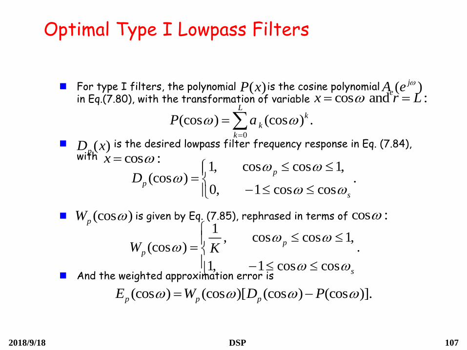
For type I filters, the polynomial is the cosine polynomial in Eq.(7.80), with the transformation of variable

is the desired lowpass filter frequency response in Eq. (7.84), with

is given by Eq. (7.85), rephrased in terms of

And the weighted approximation error is

0

(cos ) (cos ) .L

k

k

k

P a

( )P xcos and :x r L

( )pD x

(cos )pW

(cos ) (cos )[ (cos ) (cos )].p p pE W D P

Optimal Type I Lowpass Filters

( )j

eA e

cos :x 1, cos cos 1,

(cos ) .0, 1 cos cos

p

p

s

D

cos :1

, cos cos 1,(cos ) .

1, 1 cos cos

p

p

s

W K

2018/9/18 DSP 108

2018/9/18 DSP 109

2018/9/18 DSP 110

Optimal Type I Lowpass Filters

2018/9/18 DSP 111

2018/9/18 DSP 112

Type II linear phase FIR filter

2018/9/18 DSP 113

Parks-McClellan Algorithm<Type I Lowpass>

2018/9/18 DSP 114

2018/9/18 DSP 115

2018/9/18 DSP 116

2018/9/18 DSP 117

2018/9/18 DSP 118

2018/9/18 DSP 119

2018/9/18 DSP 120

Advantage and Disadvantage of FIR Design Methods

Windowing method Simplest method, and understandably conceptual design. Critical frequencies and/or ripples in frequency bands could not

manipulated into the desired precision easily. Equally ripple in each frequency band.

Frequency sampling method Technique may be selected as both recursive and non-recursive. Applicable to both typical and general filter types. Problem to manipulate band edge frequencies and passband ripple

into the desired precision.

Optimum method All of parameters can be manipulated. Coefficient calculation method is easy and efficient. For the same value of M, the result in amplitude is the best. For some filter, i.e. Hilbert transformer, differentiator, this

technique is more suitable for in comparable to another method.

2018/9/18 DSP 121

COMMENTS ON IIR AND FIR DISCRETE-TIME FILTERS

If linear phase is required FIR

If stability is required FIR (since it can be non-recursive technique)

Finite word-length effect to FIR less than IIR.

If sharp cut-off frequencies are required FIR requires more coefficients, processing time, and memory size than IIR. (However, FFT algorithm or multirate technique may be used for FIR to compensate these disadvantages.)

IIR can be used analog filter as prototype, but FIR can be synthesized more easily for any required frequency response. (However, in general, to synthesize FIR is required CAD because its algebraic design technique is very difficult.)

2018/9/18 DSP 122

IIR vs. FIR Filters

2018/9/18 DSP 123

Project of Chapter 7

Download the two audio signal files with a sampling rate of 16 KHz (one is clean and the other is noisy) from the course Web site and process the signal as follows.

Show the spectrogram of the two audio signals

Remove the noise. You need to analyze the spectrum of the noise from the two audio files and design a filter to remove the noise.