Filters and Wavelets for Dyadic Analysis - A Leading UK ... · Filters and Wavelets for Dyadic Analysis by D.S.G. Pollock University of Leicester Email: stephen [email protected]

Filters and Waveletsfor Dyadic Analysis

by D.S.G. Pollock

University of Leicester

Email: stephen [email protected]

This chapter describes a variety of wavelets and scaling functions and the mannerin which they may be generated. These continuous-time functions might be re-garded as a shadowy accompaniment—and even an inessential one—of a discrete-time wavelet analysis that can be recognised as an application of the techniques ofmulti rate filtering that are nowadays prevalent in communications engineering.

However, as the Shannon–Nyquist sampling theorem has established, there isa firm correspondence between processes in continuous time that are of boundedin frequency and their equivalent discrete-time representations. It is appropriate,therefore, to seek to uncover the continuous-time processes that might be consideredto lie behind a discrete-time wavelets analysis.

Apart from the Haar wavelet and the Shannon or sinc function wavelet, whichare polar cases that are diametrically opposed, none of the wavelets that we shallconsider have closed-form or analytic expressions. To reveal these functions, onemust pursue an iterative or recursive process, based on the two-scale dilation equa-tions, which entail the coefficients of the discrete-time filters that are associated withthe two-channel filter bank and with the pyramid algorithm of a dyadic waveletsanalysis.

The filters in question are the highpass and lowpass halfband filters that arechosen in fulfilment of the conditions of perfect reproduction and of orthogonality.The iterative procedure bequeaths these essential properties of the filters to thecontinuous-time wavelets and scaling functions.

It follows that the first step in generating a family of wavelets and scalingfunctions is to understand how to derive filters that satisfy the above-mentionedconditions. This is the concern of the first section of this chapter. A commonstating point is with the autocorrelation generating functions of the lowpass filterand of the complementary highpass filter.

These must satisfy the conditions of sequential orthogonality, individually, andthe condition of perfect reproduction, jointly. The lowpass filter is found by fac-torising the lowpass autocorrelation function, whereas the highpass filter is derivedfrom the lowpass filter in a manner that ensures that, together, the two filters willsatisfy the condition of lateral orthogonality.

1

D.S.G. POLLOCK: Filters and Wavelets

Orthogonality and Perfect Reproduction

The first concern is to derive filters that will give rise to acceptable versionsof the scaling function and the wavelet. This is a matter of finding complementaryhalfband filters that fulfil the canonical properties of perfect reconstruction and ofsequential and lateral orthogonality.

In the case of FIR filters, the conditions of orthogonality will be satisfied only byfilters with an even even number of coefficients. Such filters cannot be symmetricabout a central coefficient. Therefore, with the exception of the two-point Haarfilter, they are bound to induce a non-linear phase effect.

To see the necessity of an even number of coefficients, consider G(z) = g0 +g1z+· · ·+gM−1z

M−1 in the case where M is an odd number, as it must be for centralsymmetry. Then, if 2n = M − 1, there is p2n = g0gM−1 �= 0, since g0, gM−1 �= 0,by definition. Therefore, the condition of sequential orthogonality is violated.

Nevertheless, it is possible to obtain symmetric canonical filters that have aninfinite number of coefficients or that correspond to the circularly wrapped versionsof such filters, which are applied to circular data sequences,

In the case of the canonical FIR filter, the basic prescription is the one thatwas originally derived by Smith and Barnwell (1987). Given an appropriate halfband lowpass filter G(z), of M = 2n coefficients, the corresponding highpass filtermust fulfil the condition that

H(z) = −zM−1G(−z−1) or, equivalently, that zM−1H(−z−1) = G(z). (1)

Thus, the highpass filter is obtained from the lowpass filter by what has beendescribed an alternating flip—namely by the reversal of the sequence of coefficientsfollowed by the application of alternating positive and negative to the elements ofthe reversed sequence.

The synthesis filters to accompany these analysis filters are just their time-reversed versions:

D(z) = G(z−1) and E(z) = H(z−1). (2)

The relationship between the polynomials G(z) and H(z) can be illustratedadequately by the case where M = 4. The coefficients of the cross covariancefunction R(z) = G(z)H(z−1) can be obtained from the following table:

g0 g1z g2z2 g3z

3

h0 = g3 g3g0 g3g1z g3g2z2 g2

3z3

h1z−1 = −g2z

−1 −g2g0z−1 −g2g1 −g2

2z −g2g3z2

h2z−2 = g1z

−2 g1g0z−2 g2

1z−1 g1g2 g1g3z

h3z−3 = −g0z

−3 −g20z−3 −g0g1z

−2 −g0g2z−1 −g0g3

(3)

2


The coefficients of R(z) associated with the various powers of z are obtained bysumming the element in the rows that run in NW–SE direction. It can be seen thatr0 = 0, r2 = 0 and r−2 = 0. More generally, there is

R(z) + R(−z) = G(z)H(z−1) + G(−z)H(−z−1) = 0. (4)

This the downsampled version of the cross-covariance function, and the equationindicates that the coefficients associated with odd-valued powers of z are zeros.

In the case of symmetric IIR filters , the prescription is that, given an appro-priate lowpass filter G(z) = G(z−1), the corresponding highpass filter must fulfilthe condition that

H(z) = −z−1G(−z) or, equivalently, that H(−z) = z−1G(z). (5)

Then, the synthesis filters are

D(z) = G(z) and E(z) = −zG(−z). (6)

There is a manifest similarity in the two cases.Given these specifications, is easy to see that, if P (z) = G(z)G(−1) and Q(z) =

H(z)H(−1) then, in either case, there is

P (z) + P (−z) = G(z)G(z−1) + G(−z)G(−z−1)

= G(z)G(z−1) + H(z)H(z−1)

= H(−z)H(−z−1) + H(−z)H(−z−1) = Q(−z) + Q(z).

(7)

Given that P (z) + P (−z) = 2, in consequence of the customary the normalisationp0 = 1 of the leading coefficient of P (z), the fist equality denotes the sequentialorthogonality of the coefficient of the lowpass filter as displacements that are mul-tiples of two points. The second equality denotes the power complementarity of thetwo filters. The third equality denotes the sequential orthogonality of the highpassfilter.

Successive Approximations to a Wavelet

Except in the polar cases of the Haar wavelet and the Shannon or sinc func-tion wavelet, an explicit functional form for the wavelet or the scaling functionis unlikely to be available. Nor is there, in most practical applications, an indis-pensable requirement to represent of these functions graphically. Nevertheless, it isenlightening to examine the profiles of the wavelets and the scaling functions andto consider a method of calculating them.

Given the filter coefficients, the calculation of the wavelet depends on thebasic two–scale dilation equation. This equation expresses the scaling function atone level of resolution in terms of the functions at the twice that resolution:

φ(t) =√

2M−1∑k=0

gkφ(2t − k). (8)

3


A similar equation is expresses the corresponding wavelet in terms of the scalingfunctions:

g(t) =√

2M−1∑k=0

hkφ(2t − k). (9)

These equations have direct frequency-domain counterparts. Thus, taking theFourier transform on both sides of (8) gives

φ(ω) =∫

φ(t)e−iωtdt =√

2∫ M−1∑

k=0

gkφ(2t − k)e−iωtdt

=√

2M−1∑k=0

∫12gkφ(τ)e−iωτ/2e−iωk/2dτ

=1√2

M−1∑k=0

gke−iωk/2

∫φ(τ)e−iωτ/2dτ,

(10)

where τ = 2t had been defined, which has entailed the change of variable technique.This has introduced the factor dt/dτ = 1/2. The term exp{−ik/2} relates to thehalf-point displacements in time of the scaling functions. This equation can besummarised using

G(ω) =∑

j

gje−iωj , (11)

which is the discrete-time Fourier transform of the sequence of the coefficients ofthe dilation equation. It is also the result of setting z = exp{−iω} in G(z). Also,there is ∫ ∞

−∞φ(t)e−iωtdt = φ(ω), (12)

which is the Fourier transform of ψ(t). With these definitions, equation (19) canbe written as

φ(ω) =1√2G(ω/2)φ(ω/2), (13)

Successive approximations to the wavelet can be generated using the basictime-domain two-scale dilation equation. The iterations are defined by

φ(j+1)(t) =√

2M−1∑k=0

gkφ(j)(2t − k), (14)

were the initial value φ(0) must be given This may be specified as a unit rectangle.The frequency-domain form of the equation is seen to be

φ(j+1)(ω) =1√2G(ω/2)φ(j)(ω/2), (15)

4


The limit of successive iterations or back substitutions, if it exists, is

φ(ω) =

∞∏j=1

{1√2G

( ω

2j

)}φ(0). (16)

The Haar Wavelets

The Haar function has often been used as a didactic device for introducingthe concept of a multi resolution wavelets analysis. It has the twofold advantagethat its functional form is readily accessible and that it is easy to use in a multiresolution wavelet analysis.

The Haar wavelet has a finite support in the time domain, but it has thedisadvantage that its frequency-domain counterpart, i.e. its Fourier transform, hasan infinite support and that it has only a hyperbolic rate of decay.

An opinion that is offered in this text is that, for the purpose of capturingthe essentials of a wavelets analysis, one might as well exploit the so-called Shan-non wavelets that have characteristics that are the opposites of those of the Haarwavelets.

The Shannon wavelets, which are based on the sinc function, have a finitesupport in the frequency domain and an infinite support in the time domain. Theyhave a hyperbolic rate of decay in the time domain. They are also analytic functions.

Our description of the Haar wavelet, in this section, will be followed by thatof the Shannon wavelets in the next section. In both of these cases, closed formexpressions are available for the wavelet and the scaling functions, of which thesampled ordinates are the coefficients of the corresponding filters. Therefore, littleattention needs to be given to the lowpass autocorrelation function, which is theusual starting point in the derivation of a system of wavelets.

The Haar scaling function in V0 is given by

φ(t) ={ 1, if 0 < t < 1;

0, otherwise,(17)

and the wavelet in W0 is given by

ψ(t) =

1, if 0 < t < 1/2;

−1, if 1/2 ≤ t < 1,

0, otherwise.

(18)

The scaling function has a unit area 〈φ(t), φ(t)〉 = 1. Functions at differentinteger displacements have no overlap and they are therefore mutually orthogonalwith 〈φ(t − j), φ(t − k)〉 = δ(j − k). Thus, the set of scaling functions functions atinteger displacements provides an orthonormal, basis for the space V0.

5


For the wavelet there is, likewise, 〈ψ(t), ψ(t)〉 = 1 and 〈ψ(t − j), ψ(t − k)〉 =δ(j − k) = 0; and the set of wavelet functions at integer displacements provides anorthonormal basis for the space W0.

The wavelets and the scaling functions are laterally orthogonal, both in align-ment, and at integer displacements so that 〈ψ(t− j), φ(t− k)〉 = 0 for all j, k. Theinner product 〈φ(t), ψ(t)〉 = 0 can be seen as the average of the wavelet over theinterval [0, 1], which is clearly zero, and the functions at different displacements donot overlap.

The set of basis functions for the nested spaces Vj ; j := 0, 1, . . . , m, for whichVj+1 ⊂ Vj , are provided by the dilated scaling functions

φj,k(t) = 2−j/2φ(2−jt − k). (19)

Here, j is the so-called scale factor, which corresponds to the level of a dyadicdecomposition, whereas k is the displacement factor. The actual displacement inthe level-j wavelet ψj,k(t) is by t = 2jk points, which is its central value that solvesthe equation 2−jt − k = 0.

The basis functions for the wavelet spaces Wj ; j := 0, 1, . . . , m are provided bythe dilated wavelet function

ψj,k(t) = 2−j/2ψ(2−jt − k). (20)

The first stage of the dyadic decomposition of V0 = V1 ⊕ W1 produces adirect sum of a space of scaling functions V1 and a space wavelets W1, wherein therespective basis functions are

φ1,k(t) =1√2φ(t/2 − k) and ψ1,k(t) =

1√2φ(t/2 − k). (21)

The two-scale dilation equation for the scaling function φ1,0(t) is

φ1,0(t) =1√2φ(t/2) = g0φ(t) + g1φ(t − 1), (22)

and that of the wavelet function ψ1,0(t) is

ψ1,0(t) =1√2ψ(t/2) = h0φ(t) + h1φ(t − 1). (23)

Here,

g0 =1√2, g1 =

1√2

and h0 =1√2, h1 =

−1√2. (24)

These are the values of the ordinates sampled from the functions φ1,0(t) andψ1,0(t) at the points ε, 1 + ε, where ε ∈ (0, 1). (The inclusion of a small positivedisplacement ε is to avoid taking a sample at the jump point of ψ1,0(t) at t = 1.)They are also the values of the filter coefficients of a discrete-time analysis.

6


It will be observed that

g20 + g2

1 = 1, that h20 + h2

1 = 1 and that g0h0 + g1h1 = 0. (25)

which demonstrates that the filters can be used in constructing an orthonormalbasis for a discrete-time analysis.

Sinc Function Filters and Shannon Wavelets

The ideal halfband filters and the corresponding Shannon wavelets and scalingfunctions are realised by virtue of the sinc function. The function provides a pro-totype for a wavelet that is tractable from the point of view of its mathematicalanalysis. The wavelet and the scaling function have closed-form analytic expres-sions that leads directly, via the sampling theorem, to expressions for the filtersthat are entailed by the two-scale dilation equations.

The sinc function is defined by

φ(t) =12π

∫ π

−π

eiωtdω =12π

[eiωt

it

]π

−π

=(

eiπt − e−iπt

2πit

)=

sin(πt)πt

.

(26)

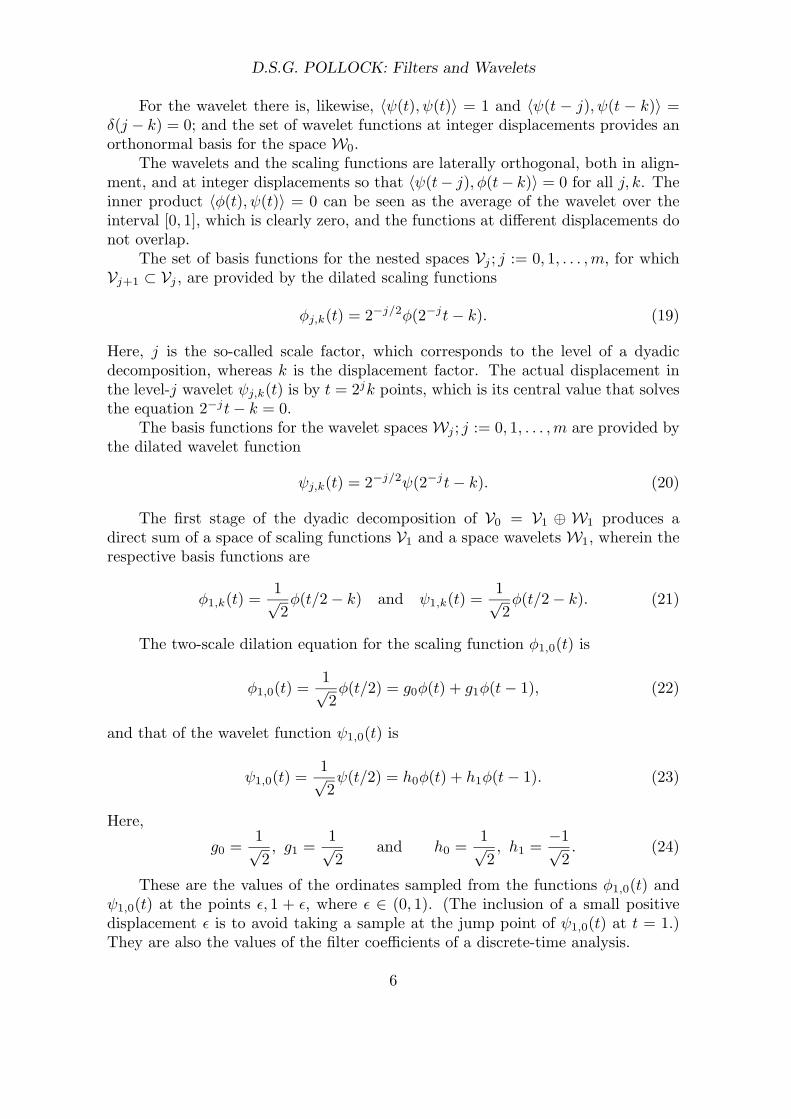
This is the (inverse) Fourier transform of a rectangle of unit height supported, in thefrequency domain, of the interval [−π, π]. The function, together with its ordinatessampled at unit intervals, is represented in Figure 1.

The sinc function gives rise to a family of scaling functions φ(t − k) thatprovide an orthonormal basis for the space V0. The sequential orthonormality ofthe functions at unit displacements follows from their fulfilment of the conditionthat ∑

k

|φ(ω + 2kπ|2 = 1, ω ∈ [−π, π], (27)

which is the frequency-domain equivalent of the condition 〈φ(t − j)φ(t − k)〉 =δ(j − k), as is indicated under (6.4).

The basis functions for the subspace V1 ⊂ V0 are given by

φ1,k(t) = 2−1/2φ(2−1t − k). (28)

Substituting the formula of (35) gives

φ1,k(t) =1√2

{sin(πt/2 − k)

πt/2

}=

√2sin(πt/2 − k)

πt. (29)

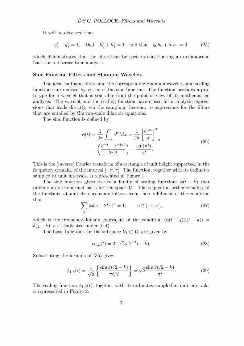
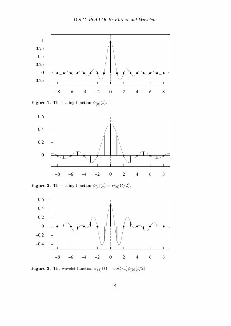
The scaling function φ1,0(t), together with its ordinates sampled at unit intervals,is represented in Figure 2.

7


0

0.25

0.5

0.75

1

0

−0.25

0 2 4 6 80−2−4−6−8

Figure 1. The scaling function φ(0)(t).

0

0.2

0.4

0.6

0

0 2 4 6 80−2−4−6−8

Figure 2. The scaling function φ(1)(t) = φ(0)(t/2).

0

0.2

0.4

0.6

−0.2

−0.4

0 2 4 6 80−2−4−6−8

Figure 3. The wavelet function ψ(1)(t) = cos(πt)φ(0)(t/2).

8


The Nyquist–Shannon sampling theorem indicates that

φ1,0(t) =∞∑

k=−∞gk

sin{π(t − k)}π(t − k)

=∞∑

k=−∞gkφ(t − k), (30)

where

gk =√

2sin(πk/2)

πt= g−k (31)

are just the ordinates sampled at unit intervals from φ1,0(t). These are also thecoefficients of the filter function

G(z) = {g0 + g1(z + z−1) + g2(z2 + z−2) + · · ·}. (32)

Equation (39) is nothing but the two-scale dilation equation for the sinc functionbases.

The sinc function sin(πk/2)/πt is idempotent. It corresponds to a rectanglein the frequency domain of unit height defined the interval [−π/2, π/2]; and thesquaring of the rectangle leaves it unaltered. The function is also symmetric, andit represents its own autocorrelation function. Thus, the conditions of sequentialorthogonality amongst the basis functions φ1,k(t) = φ(2t − k) correspond to thezeros of the sinc function, which, as can be seen from Figure 2, are at two-pointdisplacements.

A wavelet and a set of filter coefficients, to complement the scaling function of(29) and the filter coefficients of (31), may be obtained by the process of frequencyshifting that translates the φ1,k(t) in the upper frequency range [π/2, π]. Thetranslation is affected by the function cos(πt) = (−1)t.

A one-unit time lag may also be imposed in fulfilment of the condition forlateral orthogonality that applies, in general, to symmetric IIR filters. (This isnotwithstanding the fact that the scaling function and its frequency-shifted coun-terpart are already mutually orthogonal by virtue of their segregation within thefrequency domain.) Thus, the wavelet may be specified by

ψ1,k(t) = (−1)tφ1,k(t − 1) =√

2 cos(πt)sin(πt/2 − k − 1)

πt. (33)

It is represented, together with its ordinates sampled at unit intervals, by Figure 3.The corresponding filter coefficients, which are to be found in the dilation

equation

ψ1,0(t) =∞∑

k=−∞hkφ(t − k), (34)

which are just the sampled ordinates of ψ1,k(t), are given by

hk = (−1)kgk−1. (35)

9


These are also the coefficients of the filter function

H(z) = zG(−z) = z{g0 − g1(z + z−1) + g2(z2 + z−2) + · · ·}. (36)

Because its coefficients form a doubly-infinite sequence, the sinc function doesnot provide a practical filter. Also, the coefficients converge to zero slowly. Theproblems of an infinite sequence can be overcome by creating a circular filter of anorder that is appropriate to the length of the data sequence.

An alternative way of adapting the filter is to truncate the sequence. Then, toobtain a desirable frequency response, which is not affected by ripples or by exces-sive leakage, it is appropriate to apply a taper to the coefficients via a symmetricsequence of weights {wj ; j = 0,±1, . . . ,±M − 1}, with wj = w−j and w0 = 1.

The generic element of the weighted and truncated autocorrelation sequencemay be denoted by

pj =

wj2 sin(πj/2)

πj, for j = 0,±1, . . . ,±M − 1;

0, otherwise,(37)

Given that the sinc function already satisfies the conditions of sequential orthogo-nality, which is that the coefficients of P (z) associated with even powers of z arezeros, it follows that, regardless of the choice of the weights, the weighted functionwill also satisfy the conditions.

For an appropriate weighting function, one might think of using the Blackmanwindow (see Blackman and Tukey 1959) which is defined by

wj = 0.42 + 0.5 cos(πj

M

)+ 0.08 cos

(2πj

M

), where |j| ≤ M − 1. (38)

An alternative weighting function is provided by the split cosine bell defined by

wj =

0.5

[1 + cos

π(M + j)q

]; j = 1 − M, . . . , q − M,

1.0; j = q − M, . . . , M − q,

0.5[1 + cos

π(q − M + j)q

]; j = M − q, . . . , M − 1.

(39)

This has a horizontal segment interpolated at the apex of the bell. Setting q = Mreduces this to the cosine bell.

If the autocorrelation function P (z) is to be amenable to a spectral factorisationsuch that P (z) = G(z)G(z−1), then it is necessary that P (ω) > 0 for all ω ∈ [−π, π].If this is not the case and if minP (ω) = q < 0, then P (z) can be replaced by P (z)−q.The autocorrelation function can be rescaled so as to satisfy the condition thatP (z) + P (−z) = 2.

10


Once an appropriate positive-definite symmetric function is available, it can befactorised to give the function G(z), which has an even number M of coefficients.Thereafter, the highpass filter H(z) = −zM−1G(−z−1) can be obtained by meansof a signed reversal.

A numerical procedure for the spectral factorisation of the autocorrelationfunction has been provided by Tunnicliffe Wilson (1969) and it has been codedin Pascal and C by Pollock (1999). A discourse on the alternative methods forfactorising a Laurent polynomial has been provided by Goodman et al. (1997).

Infinite Impulse Response Filters

One way of satisfying the condition of perfect reconstruction is to exploit thestructure of the Wiener–Kolmogorov filters to derive a pair of complementary half-band filters. Let F (z) be an arbitrary polynomial. Then, the autocorrelationfunction of the lowpass filter can take the form of

P (z) =2F (z)F (z−1)

F (z)F (z−1) + F (−z)F (−z−1); (40)

and this may be factorised as P (z) = G(z)G(z−1). It is easy to see that P (z) +P (−z) = 2, whereby the condition of perfect reconstruction is confirmed. The filtermay be subject to an arbitrary number of translations in time that can be effectedby an allpass filter or by a power of z. In that case, we may assume the factoraffecting the translation is absorbed within the function G(z). The correspondinghighpass filter will be H(z) = −z−1G(−z).

A familiar example of such an autocorrelation function is provided by

P (z) =2(1 + z)n(1 + z−1)n

(1 + z)n(1 + z−1)n + (1 − z)n(1 − z−1)n

=2

1 +(

i1 − z

1 + z

)2n ,(41)

which is the formula of the lowpass halfband Butterworth filter. The second expres-sion is derived by dividing top and bottom of the first expression by the numerator.Then, the top and bottom of each factor within {(1−z−1)/(1+z−1)}n are multipliedby z. The factor i2n provides n changes of sign.

The roots of P (z), i.e. its poles and its zeros, come in reciprocal pairs; and,once they are available, they may be assigned unequivocally to the factors G(z)and G(z−1). Those roots which lie outside the unit circle belong to G(z) whilsttheir reciprocals, which lie inside the unit circle, belong to G(z−1).

The zeros of P (z) are already available. To find the poles, consider the equation

(1 + z)n(1 + z−1)n + (1 − z)n(1 − z−1)n = 0, (42)

11


which is equivalent to the equation

1 +(

i1 − z

1 + z

)2n

= 0. (43)

Solving the latter for

s = i1 − z

1 + z(44)

is a matter of finding the 2n roots of −1. These are given by

s = exp{ iπj

2n

}, where j = 1, 3, 5, . . . , 4n − 1,

or j = 2k − 1; k = 1, . . . , 2n.(45)

The roots correspond to a set of 2n points which are equally spaced around thecircumference of the unit circle. The radii that join the points to the centre areseparated by angles of π/n; and the first of the radii makes an angle of π/(2n) withthe horizontal real axis.

The inverse of the function s = s(z) is the function

z =i − s

i + s=

i(s − s∗)2 − i(s∗ − s)

, (46)

Here, the final expression comes from multiplying top and bottom of the secondexpression by s∗ − i = (i + s)∗, where s∗ denotes the conjugate of the complexnumber s, and from noting that ss∗ = 1. On substituting the expression for s from(34), it is found that the solutions of (34) are given, in terms of z, by

zk = icos{π(2k − 1)/2n}

1 + sin{π(2k − 1)/2n} , where k = 1, . . . , 2n. (47)

The roots of G(z−1) = 0 are generated when k = 1, . . . , n. Those of G(z) = 0 aregenerated when k = n + 1, . . . , 2n.

Given the availability of the analytic expressions for the roots of the Butter-worth polynomial, we might hope to find a straightforward factorisation of thefunction P (z) = G(z)G(z−1) that does not require an iterative procedure.

Herley and Vetterli (1993) have demonstrated that, in the special case whereF (z) is of an even length and when it comprises a symmetric sequence of coefficients,there is indeed a simple closed form factorisation of P (z) that is available moregenerally to other versions of the Weiner–Kolmogorov function.

Consider, therefore, a causal filter

F (z) = f0 + f1z + · · · + f1zN−1 + f0z

N . (48)

which has a even number N +1 of terms that form a symmetric sequence. Since thenumber of terms is even, there is no central point of symmetry within the sequence.

12


The terms associated with the even and the odd powers of z can be separatedto form the polynomials

Fe(z2) = f0 + f2z2 + · · · + f1z

N−1, Fo(z2) = f1 + f3z2 + · · · + f0z

N−1, (49)

for which Fo(z2) = zN−1Fe(z−2). Then, it follows that

F (z) = Fe(z2) + zFo(z2) = Fe(z2) + zNFe(z−2). (50)

Therefore,

F (z)F (z−1) = {Fe(z2) + zNFe(z−2)}{Fe(z−2) + z−NFe(z2)}= 2Fe(z2)Fe(z−2)

+ {zNFe(z2)Fe(z−2) + z−NFe(z2)Fe(z−2)}.(51)

SinceF (z)F (z−1) + F (−z)F (−z−1) = {F (z)F (z−1)}e (52)

contains only even powers of z, and since N is an odd number, it follows that

{F (z)F (z−1)}e = 2Fe(z2)Fe(z−2) (53)

Therefore, the function of (31) can be expressed as

P (z) =F (z)F (z−1)

Fe(z2)Fe(z−2)(54)

of which the requisite factor is

G(z) =F (z)

Fe(z2). (55)

The function that provides the frequency-domain profile of the Butterworthfilter is obtained by setting z = e−iω in (43). In that case,

1 +(

i1 − z

1 + z

)2n

= 1 +(

iz−1/2 − z1/2

z−1/2 + z1/2

)2n

= 1 +{

sin(ω/2)cos(ω/2)

}2n

, (56)

since sin(ω/2) = −i{exp(iω/2) − exp(−iω/2)}/2 and cos(ω/2) = {exp(iω/2) +exp(−iω/2)}/2. Therefore, the function in question is

P (ω) = {1 + tan(ω)2n}−1. (57)

13


Filtering in the Frequency Domain

Within the time domain, filters are applied to the data via a process of con-volution. If the data and the filter sequences are lengthy, then this may be acomputationally demanding and a time consuming process. On the other hand, ifthe data sequence is short relative to the length of the filter, then there is liable tobe a significant end-or-sample problem.

Provided that one is able to perform the computations off-line, then bothproblems can be addressed by performing the operations in the frequency domain.The time-consuming process of convolution in the time domain is converted into amore efficient process of modulation in the frequency domain, whereby the Fouriertransforms of the data and the filter are multiplied together point by point.

The end-of-sample problem is handled automatically by the process offrequency-domain modulation, which corresponds to an application of circular con-volution in the time domain. The latter would entail using the initial sample valuesas proxies for the values that lie beyond the end of the sample and using the finalsample values as proxies for the presample values.

Provided that the data have been adequately detrended, there may be littleharm in such a contrivance. What harm there might be can be mitigated by theprovision of some carefully constructed synthetic data to be interpolated into thecircular data sequence, where the end joins the beginning.

The essential condition that must be fulfilled by the frequency-domain versionsof the wavelets filters is that of power complementarily whereby

P (ω) + Q(ω) = |G(ω)|2 + |H(ω)|2 = 2. (58)

Moreover, if the functions P (ω)and Q(ω) are to be mirror images of each other,then it must be that Q(ω) = P (ω + π). The latter requires the functions to bereflections of each other about the about the vertical axis through π/2 and aboutthe horizontal axis of unit height.

The condition

|G(ω)|2 + |G(ω + π)|2 = 2, (59)

which comes from setting H(ω) = G(ω + π) in (41) can also be deduced from thecondition that ∑

k

|φ(ω + 2kπ|2 = 1. (60)

As was indicated under (6.4), this is the frequency-domain equivalent of the condi-tion othonormality affecting the family of scaling functions φ(t−k). The frequency-domain version of the dilation equation is

φ(ω) = 2−1/2G(ω/2)φ(ω/2), (61)

14


and substituting this into (69) gives

1 =12

∑k

|G(ω + kπ)|2|φ(ω + kπ)|2

=12|G(ω)|2

∑k

|φ(ω + 2kπ)|2

+12|G(ω + π)|2

∑k

|φ(ω + [2k + 1]π)|2

=12

{|G(ω)|2 + |G(ω + π)|2

}(62)

The condition of (60) is fulfilled, of course, by the Shannon filter defined under(29) which corresponds to a perfect rectangular halfband frequency response. How-ever, this function has a slow hyperbolic rate of convergence as well as an infinitesupport in the time domain.

The difficulty of the infinite support can be overcome by the circular wrappingof the filter, which occurs when the frequency-domain rectangle is sampled at Tpoints which are transformed via the inverse discrete Fourier transform to createcircular filter.

The difficulty of the slow convergence of the Shannon wavelets is attributableto the sharp frequency cut-off at π/2. It can be addressed by imposing a moregradual transition from the pass band to the stop and vice versa.

There are numerous pairs of functions with more or less gradual transitionsthat satisfy the power complementary condition of (59). The simplest are derivedby placing a cross at the points ±π/2. The resulting power spectrum of the lowpass filter, which may be described as a split triangle or as a chamfered box, isdefined by

P (ω) =

1, if |ω| ∈ (0, π/2 − ε),

1 − |ω + ε − π/2|2ε

, if |ω| = (π/2 − ε, π/2 + ε),

0, otherwise.

(63)

Setting ε = π/2 reduces this to a triangular function. Also subsumed underthis function is the rectangular function The discontinuity at the cut-off point ishandled, in effect, by chamfering the edge. (When the edge of the box is chamferedin the slightest degree, the two function values at the point of discontinuity, whichare zero and unity, will coincide at a value of one half.) The result can be a greatlyimproved rate of convergence; but this crude recourse fails achieve an optimal tradeoff between dispersion in the time domain and dispersion in the frequency domain,

A superior recourse is to use the Butterworth function of (57) to obtain awide range of profiles for the power function P (ω). There is no reason why, inthis context, the parameter n should be restricted to take an integer value. It willbe found, for example that when n = 0.65 the Butterworth function provides a

15


0

0.25

0.5

0.75

1

−π −π/2 0 π/2 π

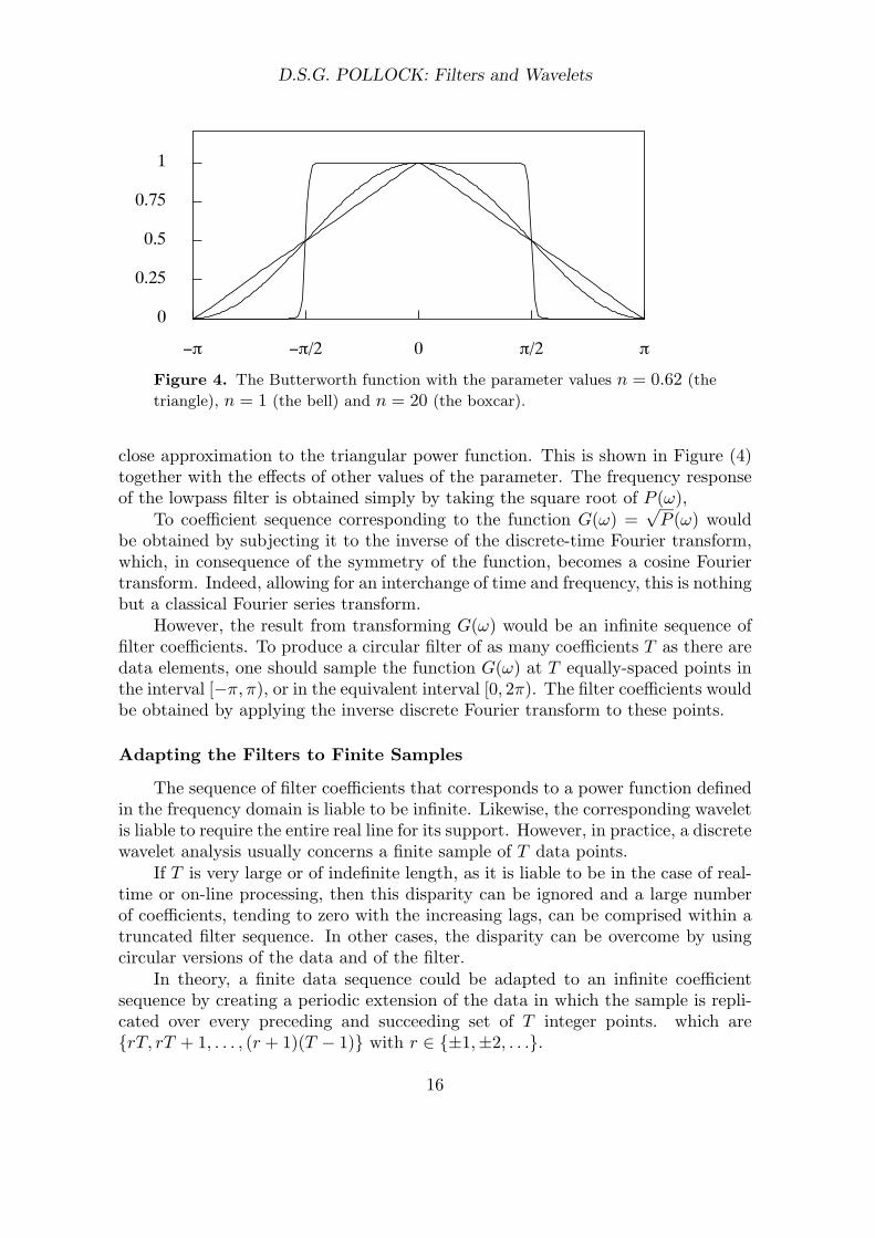
Figure 4. The Butterworth function with the parameter values n = 0.62 (the

triangle), n = 1 (the bell) and n = 20 (the boxcar).

close approximation to the triangular power function. This is shown in Figure (4)together with the effects of other values of the parameter. The frequency responseof the lowpass filter is obtained simply by taking the square root of P (ω),

To coefficient sequence corresponding to the function G(ω) =√

P (ω) wouldbe obtained by subjecting it to the inverse of the discrete-time Fourier transform,which, in consequence of the symmetry of the function, becomes a cosine Fouriertransform. Indeed, allowing for an interchange of time and frequency, this is nothingbut a classical Fourier series transform.

However, the result from transforming G(ω) would be an infinite sequence offilter coefficients. To produce a circular filter of as many coefficients T as there aredata elements, one should sample the function G(ω) at T equally-spaced points inthe interval [−π, π), or in the equivalent interval [0, 2π). The filter coefficients wouldbe obtained by applying the inverse discrete Fourier transform to these points.

Adapting the Filters to Finite Samples

The sequence of filter coefficients that corresponds to a power function definedin the frequency domain is liable to be infinite. Likewise, the corresponding waveletis liable to require the entire real line for its support. However, in practice, a discretewavelet analysis usually concerns a finite sample of T data points.

If T is very large or of indefinite length, as it is liable to be in the case of real-time or on-line processing, then this disparity can be ignored and a large numberof coefficients, tending to zero with the increasing lags, can be comprised within atruncated filter sequence. In other cases, the disparity can be overcome by usingcircular versions of the data and of the filter.

In theory, a finite data sequence could be adapted to an infinite coefficientsequence by creating a periodic extension of the data in which the sample is repli-cated over every preceding and succeeding set of T integer points. which are{rT, rT + 1, . . . , (r + 1)(T − 1)} with r ∈ {±1,±2, . . .}.

16


By these means, the data value at a point t /∈ {0, 1, . . . , T−1}, which lies outsidethe sample, is provided by yt = y{t mod T}, which does lie within the sample. Withthe periodic extension available, one can think multiplying the filter coefficientspoint by point with the data and of shifting them any number of times.

As an alternative to extending the data, one can think of creating a finitesequence of filter coefficients by wrapping the infinite filter sequence {gt} around acircle of circumference T and adding the overlying coefficients to give

g◦t =∞∑

k=−∞g{t+kT} for t = 0, 1, . . . , T − 1. (64)

The inner product of the resulting coefficients g◦0 , . . . , g◦T−1 with a finite se-quence x0, . . . , xT−1 will be identical to that of the original coefficients with theextended sequence. To show this, let x̃(t) = {x̃t = x{t mod T}} denote the infinitesequence that is the periodic extension of x0, . . . , xT−1. Then

∞∑t=−∞

gtx̃t =∞∑

k=−∞

{T−1∑t=0

g{t+kT}x̃{t+kT}

}

=T−1∑t=0

xt

{ ∞∑k=−∞

g{t+kT}

}=

T−1∑t=0

g◦t xt.

(65)

Here, the first equality, which is the result of cutting the sequence {gtx̃t} intosegments of length T , is true in any circumstance, whilst the second equality usesthe fact that x̃{t+kT} = x{t mod T} = xt. The final equality invokes the definitionof g◦t .

In fact, the process of wrapping the filter coefficients should be conducted inthe frequency domain, where it is simple and efficient, rather than in the the timedomain, where it entails the summation of an infinite sequence. We shall elucidatethese matters while demonstrating the use of the discrete Fourier transform inperforming a wavelt analysis.

To elucidate these matters, consider the z-transforms of the filter sequence andthe data sequence:

G(z) =∞∑

t=−∞gtz

t and x(z) =T−1∑t=0

xtzt. (66)

Setting z = exp{−iω} in G(z) creates a periodic function in the frequency do-main of period 2π, denoted by g(ω), which, by virtue of the discrete-time Fouriertransform, corresponds one-to-one with the doubly infinite time-domain sequenceof filter coefficients.

Setting z = zj = exp{−i2πj/T}; j = 0, 1, . . . , T −1, is tantamount to samplingthe continuous function G(ω) at T points within the frequency range of ω ∈ [0, 2π).

17


(Given that the data sample is defined on a set of positive integers, it is appro-priate to replace the symmetric interval [−π, π], considered hitherto, in which theendpoints are associated with half the values of their ordinates, by the positivefrequency interval [0, 2π), which excludes the endpoint on the right and attributesthe full value of the ordinate at zero frequency to the left endpoint.) The powersof zj now form a T -periodic sequence, with the result that

G(zj) =∞∑

t=−∞gtz

tj (67)

={ ∞∑

k=−∞gkT

}+

{ ∞∑k=−∞

g(kT+1)

}zj + · · · +

{ ∞∑k=−∞

g(kT+T−1)

}zT−1j

= g◦0 + g◦1zj + · · · + g◦T−1zT−1j = G◦(zj).

There is now a one-to-one correspondence, via the discrete Fourier transform, be-tween the values G(zj); j = 0, 1, . . . , T − 1, sampled from G(ω) at intervals of2π/T , and the coefficients g◦0 , . . . , g◦T−1 of the circular wrapping of g(t). Settingz = zj = exp{−i2πj/T}; j = 0, 1, . . . , T −1, within y(z) creates the discrete Fouriertransform of the data sequence, which is commensurate with the square roots ofthe ordinates sampled from the energy function.

The Daubechie Maxflat FIR Filters

The filters that have come to dominate dyadic wavelets analysis are the onesthat have been proposed by Daubechies (1988, 1992). These are the so-calledmaxflat halfband FIR filters that entail an even number M = 2m of coefficients ofwhich z-transforms constitute polynomials of degree M − 1. The lowpass scalingfunction filter G(z) and the highpass wavelets filter H(z) form a power complemen-tary pair of which the sum of the squared gain functions is a constant function:

G(z)G(z−1) + H(z)H(z−1) = 2 (68)

A maxflat condition is fulfilled when there is a maximum number of zero-valued derivatives at a specific point or set of points in the frequency response.The condition that is imposed on the lowpass filter, of which the z-transform isG(z) = g0 + g1z + · · ·+ gM−1z

M−1, is that the response has the maximum numberof zeros at the point z = −1, which correspond to factors of 1 + z within G(z).

Once the lowpass filter has been specified, the condition of sequential orthog-onality requires that the highpass filter should be

H(z) = −zM−1G(−z−1). (69)

Therefore, the maxflat condition affecting G(z) imposes the same number of zeroson H(z) at the point z = 1, which correspond to factors of 1 − z. Given that the

18


two filters are complementary, the two sets of maxflat conditions imply that thetwo filters have flat frequency responses both at z = 1 and at z = −1.

The filter G(z) is derived by factorising the autocovariance function P (z) =G(z)G(z−1), which has 4m−1 coefficients associated with powers of z ranging from1 − 2m to 2m − 1.

The conditions of sequential orthogonality require that P (z) has 2m − 2 zero-valued coefficients: p2j = 0; j = ±1, . . . ,±(m−1). There is also a central coefficientwith the value of p0 = 1. This leaves a reminder of 2m coefficients that can beused in placing zeros in P (z) at ω = π, which correspond to polynomial roots atz = z−1 = exp{±iπ} = −1. In that case, the autocovariance function must takethe form of

P (z) = G(z)G(z−1) =(

1 + z

2

)m

W (z)(

1 + z−1

2

)m

, (70)

where W (z) = W (z−1) is a symmetric polynomial of 2m−1 coefficients, associatedwith powers of z running from 1 − m to m − 1. This can be factorised as W (z) =V (z)V (z−1), whereafter G(z) = {(1 + z)/2}mV (z) can be formed.

Observe that the presence of the operator (1 − z)m within H(z) implies thethis filter will nullify the ordinates of polynomial of degree m − 1. Therefore, thecondition of perfect reproduction, which is a feature of an orthogonal filter bank,implies that G(z) will transmit the ordinates of the polynomial.

The factors of W (z) can be obtained via an iterative procedure, but, in somesimple cases, it is possible to perform the factorisation analytically as the followingexample shows, which concerns the Daubechies D4 filter. This is a filter of length4 that satisfies the conditions of sequential and lateral orthogonality.

Example. Let m = 2 and let W (z) = αz−1 + β + αz. On compounding this withthe factors {(1 + z)/2}2 = {1 + 2z + z2}/4 and {(1 − z)/2}2, we get

P (z) = {αz−3 + (4α + β)z−2 + (7α + 4β)z−1 + (8α + 6β)

+ (7α + 4β)z + (4α + β)z2 + αz−3}/16.(71)

The conditions of sequential orthogonality indicate that the coefficients associatedwith z2 and z−2 are zeros. The coefficient associated with z0 is unity. Therefore,

4α + β = 0 and 8α + 6β = 16. (72)

The solutions of these equations are

α = −1 and β = 4, (73)

and W (z) = V (z)V (z−1) becomes

W (z) = −z−1 + 4 − z

=12({1 +

√3} + {1 −

√3}z−1)({1 +

√3} + {1 −

√3}z).

(74)

19


It follows that the lowpass filter G(z) = {(1 + z)/2}2V (z) is given by

G(z) =(

14√

2

)(1 + z)2({1 +

√3} + {1 −

√3}z)

=(

14√

2

)({1 +

√3} + {3 +

√3}z + {3 −

√3}z2 + {1 −

√3}z3).

(75)

The Method of Daubechies

The original approach pursued by Daubechies in deriving maxflat filter ofhigher orders was somewhat complicated. It has the virtue, nevertheless, of iden-tifying the functional form, in general, of the polynomial V (z) within G(z) ={(1 + z)/2}mV (z).

To begin, one may consider the expressions for P (z) = G(z)G(z−1) and P (−z)that incorporate the zeros at z = −1 and at z = 1 respectively. These are

P (z) =(

1 + z

2

)m

W (z)(

1 + z−1

2

)m

and

P (−z) =(

1 − z

2

)m

W (−z)(

1 − z−1

2

)m

.

(76)

Setting z = exp{−iω} within(1 + z

2

) (1 + z−1

2

)=

12

{1 +

z + z−1

2

}=

{z1/2 + z−1/2

2

}2

(77)

gives

1 + cos(ω)2

= cos2(ω/2) = 1 − y. (78)

Replacing z in (77) by −z and again setting z = exp{−iω} gives

1 − cos(ω)2

= sin2(ω/2) = y. (79)

Therefore, the condition for sequential orthogonality, which is that P (z)+P (−z) =2, can be expressed as

2 = P (ω) + P (ω + π)

={

cos2(ω

2

)}m

W (ω) +{

sin2(ω

2

)}m

W (ω + π).(80)

Next, it is recognised that the functions W (z) and W (−z) with z = exp{−iω} canbe expressed as trigonometrical polynomials:

W (ω) = Q(sin2{ω/2}), W (ω + π) = Q(cos2{ω/2}). (81)

20


Therefore, on setting sin2{ω/2) = y and cos2{ω/2) = 1 − y, equation (80) can bewritten as

2 = (1 − y)mQ(y) + ymQ(1 − y). (82)

Now, the object is to find a solution to the polynomial Q(y), which will lead toW (z) = V (z)V (z−1) and thence to G(z). To this end, it is appropriate to considerthe equation

1 = {(1 − y) + y}2m−1

=2m−1∑j=0

(2m − 1

j

)(1 − y)jy2m−1−j

=m−1∑j=0

(2m − 1

j

)(1 − y)jy2m−1−j +

2m−1∑j=m

(2m − 1

j

)(1 − y)jy2m−1−j .

(83)

Using (2m − 1

j

)=

(2m − 1

2m − 1 − j

)=

(2m − 1)!j!(2m − 1 − j)!

and defining k = 2m − 1 − j enables us to rewrite the second term of (91) as

m−1∑k=0

(2m − 1

k

)yk(1 − y)2m−1−k, (84)

whence, on multiplying by 2, equation (83) becomes

2 =ym2m−1∑j=0

(2m − 1

j

)(1 − y)jym−1−j

+ (1 − y)m2m−1∑j=0

(2m − 1

j

)yj(1 − y)m−1−j

=ymQ(1 − y) + (1 − y)mQ(y),

(85)

where

Q(y) = 2m−1∑j=0

(2m − 1

j

)yj(1 − y)m−1−j . (86)

Here, we may observe that Q(y) is a polynomial of degree m − 1, which maybe indicated by denoting it by Qm−1(y). It is straightforward to show that

12 Q0(y) = 1,

12 Q1(y) = 1 + 2y,

12 Q2(y) = 1 + 3y + 6y2,

12 Q4(y) = 1 + 4y + 10y2 + 20y3.

(87)

21


An easy means of generating such coefficients is illustrated by the following matrix:1 1 1 11 2 4 41 3 6 101 4 10 20

. (88)

Here, as one moves from left to right, the elements of each column after the firstare formed via a running total of the elements of the previous column. Also, thesuccessive matrix diagonals of a NE–SW orientation contain the coefficients fromsuccessive rows of Pascal’s triangle.

An alternative form for Q(y) can be found by considering the matter of solvingto equation (82) directly. The solution must satisfy the equation

Q(y) = (1 − y)−m{2 − ymQ(1 − y)}, (89)

and, given that it is a polynomial of degree m−1, this is bound to comprise the firstm terms of the expansion of (1 − y)−m. The higher order terms of the expansionwill be cancelled with terms within ymQ(1 − y). The coefficient of yk within theTaylor series or binomial expansion of (1 − y)−m is

m(m + 1) · · · (m + k − 1)k!

=(m + k − 1)!k!(m − 1)

=(

m + k − 1k

). (90)

Therefore, the alternative expression for the solution is

Q(y) = 2m−1∑k=0

(m + k − 1

k

)yk. (91)

It is easy to recognise that this also generates the equations of (87) and that thecoefficients of the expansion of (1− y)−m are the elements of the mth column of anindefinitely extended version of the matrix of (87).

Now, by setting y = sin2(ω/2) and 1 − y = cos2(ω/2) within the equation(1 − y)mQ(y) and using the identities of (78) and (79), it can be seen that

P (ω) = 2(

1 + cos(ω)2

)m m−1∑k=0

(m + k − 1

k

) (1 − cos(ω)

2

)k

, (92)

which can also be rendered as

P (ω) = 2(

1 + z

2

)m (1 + z−1

2

)m m−1∑k=0

(m + k − 1

k

) (1 + z

2

)k (1 + z−1

2

)k

.

(93)

22


References

Blackman , R.B., and T.W. Tukey, (1959), The Measurement of the Power Spectrumfrom the Point of View of Communications Engineering, Dover Publications, NewYork.

Daubechies, I., (1988), Orthonormal Bases of Compactly Supported Wavelets,Communications on Pure and Applied Mathematics, 41, 909–996.

Daubechies, I., (1992), Ten Lectures on Wavelets, Vol. 61 of CBMS-NSF RegionalConference Series in Applied Mathematics, SIAM, Philadelphia.

Goodman, T.N.T., C. Micchelli, G. Rodriguez and S. Seatzu, (1997), Spectral Fac-torization of Laurent Polynomials, Advances in Computational Mathematics, 7,429–454.

Herley, C., and M. Vetterli, (1993), Wavelets and Recursive Filter banks, IEEETransactions on Signal Processing, 41, 2536–2556.

Pollock, D.S.G,, (1999), A Handbook of Time-Series Analysis, Signal Processingand Dynamics, Academic Press, London.

Smith M.J.T., and T.P. Barnwell III, (1987), A New Filter Bank Theory for Time-frequency Representation, IEEE Transactions on Acoustics Speech and Signal Pro-cessing, 35, 314–327.

Vaidyanathan, P.P., (1985), On Power-complementary FIR Filters, IEEE Transac-tions on Circuits and Systems, 32, 1308–1310.

Vaidyanathan, P.P., P. Regalia and S.K. Mitra, (1986), Design of Doubly Com-plementary IIR Digital Filters, Using a Single Complex Allpass Filter, IEEE In-ternational Conference on Acoustics, Speech and Signal Processing, (ICASSP ’86),2547–2550.

Wilson, G.T., (1969), Factorisation of the Covariance Generating Function of aPure Moving Average Process, SIAM Journal of Numerical Analysis, 6, 1–7.

23

Documents

Filters and Wavelets for Dyadic Analysis - A Leading UK ... · Filters and Wavelets for Dyadic Analysis by D.S.G. Pollock University of Leicester Email: stephen [email protected]