Embed Size (px)
Citation preview

1
FINAL REPORT OF CCM KEY COMPARISON OF MASS STANDARDS CCM.M-K6, 50 kg
1 Patrick J. Abbott, 2 Luis O. Becerra, 3 Michael Borys, 4 Stuart Davidson, 5 Claude Jacques, 6 Sungjun Lee, 7 Víctor Loayza, 8 Andrea Malengo and 9 Ma. Nieves Medina
1 National Institute of Standards and Technology (NIST) – Gaithersburg Maryland, UNITED STATES
OF AMERICA 2 Centro Nacional de Metrología (CENAM) – Querétaro, MEXICO 3 Physikalisch-Technische Bundesanstalt (PTB) – Braunschweig, GERMANY 4 National Physical Laboratory (NPL) – Teddington, UNITED KINGDOM 5 National Research Council (NRC) – Ottawa Ontario, CANADA K1A 0R6 6 Korea Research Institute of Standards and Science (KRISS) – Daejeon, KOREA 7 Instituto Nacional de Metrologia, Qualidade e Tecnologia (INMETRO) – Duque de Caxias, Rio de
Janeiro, BRAZIL 8 Istituto Nazionale di Ricerca Metrologica (INRIM) – Torino, ITALY 9 Centro Español de Metrología (CEM) – Tres Cantos Madrid, SPAIN
ABSTRACT In order to show equivalence in mass standards calibration among National Metrology Institutes of member countries of the “Comité international des poids et mesures” (CIPM), key comparisons of mass standards have been carried out under the auspices of the “Comité Consultatif pour la Masse et les Grandeurs Apparentées” (CCM). This key comparison on 50 kg standards in standard stainless steel was based on the decision of the CCM during the 11th meeting held in April 2008 at the “Bureau International des Poids et Mesures” (BIPM). For this key comparison CENAM – Mexico acted as pilot laboratory, and NPL – United Kingdom accepted to be co-pilot laboratory. The aims of this key comparison were to compare the results obtained by NMIs in calibration of 50 kg stainless steel weights and to repeat the exercise realized in 2001 – 2002 with the key comparison identified as CCM.M-K3. 1. INTRODUCTION The CCM.M-K6 comparison was based on the decision of the CCM during the 11th meeting held in April 2008 at the BIPM. The comparison was piloted by CENAM and NPL acted as co-pilot laboratory, the comparison was organized in two petals, and used two 50 kg stainless steel standards. Nine laboratories measured at least one of the travelling standards between April 2011 and July 2013.

2
The median from mass differences between results of participant laboratories and results reported by pilot laboratory was calculated, and this median was used as the reference value for this key comparison. The mass differences between results reported by participant laboratories and the reference value were evaluated as well as the mass differences between any pair of participant laboratories. Even when these mass differences between any pair of participant laboratories are no longer required to publish in KCDB, these mass differences are presented in this report as additional information, see 7.4.2. In order to estimate the reference value and all mass differences, a numerical simulation was done. 2. PARTICIPANTS
Nine National Metrology Institutes took part of this key comparison. Among the participants, four are SIM1 members, four are EURAMET2 members and one is APMP3 member. The participating laboratories are listed in table 1.
Table 1. Participant laboratories of the comparison
National Institute of Metrology Acronym Country
Instituto Nacional de Metrologia, Qualidade e Tecnologia
INMETRO Brazil
Centro Nacional de Metrología CENAM Mexico
National Physical Laboratory NPL United Kingdom
Korea Research Institute of Standards and Science
KRISS Korea
Istituto Nazionale di Ricerca Metrologica INRIM Italy
Physikalisch-Technische Bundesanstalt PTB Germany
National Research Council Canada NRC Canada
Centro Español de Metrología CEM Spain
National Institute of Standards and Technology NIST United States of America
1 Sistema Interamericano de Metrología
2 European Association of National Metrology Institutes
3 Asia Pacific Metrology Programme

3
3. MASS COMPARATOR USED BY PARTICIPANTS The weighing instruments used by participating laboratories are listed in table 2.
Table 2. Weighing Instruments used by participant laboratories.
Acronym Manufacturer Type Range Resolution
INMETRO Mettler -Toledo AX64000 64 kg 0.1 mg
CENAM Mettler-Toledo AX64000 64 kg 0.1 mg
NPL Mettler-Toledo AX64000 64 kg 0.1 mg
KRISS Sartorius CC50001S-L 50 kg 1 mg
INRIM INRIM
Equal arms, electromagnetic compensation
4 positions
10 kg - 50 kg 0.15 mg
PTB Mettler-Toledo AX64000 64 kg 0.1 mg
NRC Sartorius C50000S 50 kg 1 mg
CEM Mettler-Toledo AX64000 64 kg 0.1 mg
NIST Mettler-Toledo AX64000 64 kg 0.1 mg
Note: Certain commercial equipment, instruments, or materials are identified in this paper to foster understanding. Such identification does not imply recommendation or endorsement by any of the participating organizations nor does it imply that the materials or equipment identified are necessarily the best available for the purpose 4. TRAVELLING STANDARDS The travelling standards for this comparison were two 50 kg weights, each made in one piece of stainless steel, cylindrical shaped (Fig. 1).
Fig. 1. Travelling standard

4
4.1 Carrying case for the transportation of the travelling standards The travelling standards were sent to the participant laboratories in plastic boxes as outer containers, inside were placed the inner containers made in aluminium, where the travelling standards were placed.
Fig. 2. Outer container for the travelling standard
Fig. 3. Inner container made in aluminium
Fig. 4. Aluminium case containing the travelling
standard
Fig. 5. Travelling standard

5
4.2 Characterization of the travelling standards Values of volume, density and magnetic properties of the weights were measured at CENAM before their circulation among participant laboratories. The data of the travelling standards are listed in table 3.
Table 3. Data of the travelling standards
Identification K6-01 K6-02
Nominal Value 50 kg 50 kg
Density at 20 ºC * 7 949.75 kg/m3 7 964.49 kg/m
3
Standard uncertainty of the density
0.28 kg/m3 0.28 kg/m
3
Volume at 20 ºC * 6 289.50 cm3 6 277.87 cm
3
Standard uncertainty of the volume
0.22 cm3 0.22 cm
3
Magnetic susceptibility (𝝌) *
< 0.01 < 0.01
Magnetization * < 1 µT < 1 µT
Surface roughness Rz
< 0.5 µm < 0.5 µm
Surface roughness Ra
< 0.1 µm < 0.1 µm
Height 288 mm 288 mm
Diameter 185 mm 185 mm
Height of centre of gravity above base
124.7 mm 124.7 mm
* Values measured by the pilot laboratory. 5. CIRCULATION OF THE TRAVELLING STANDARDS For this comparison the two weights were circulated among participants in two petals according to dates listed in table 4 and 5. One 50 kg weight was circulated within each petal. At the beginning, both travelling standards were measured at CENAM and NPL. These measurements were used to link the results of participating laboratories of both petals. CENAM measured the mass of the standards at the beginning and at the end of the circulation in order to evaluate their possible drift. The differences between the results of CENAM and NPL in both standards were used to evaluate the reproducibility of CENAM results. An intermediate measurement made by pilot laboratory was required for the travelling standard K6-01 (petal 1) since the control over it was lost during its transfer between Canada and United States. No significant drift was found in the calibration of this travelling standard. For the circulation of the travelling standard for petal 2, K6-02, no remarkable incidents occurred.

6
Table 4. Petal 1, Circulation of the standard K6-01 Acronym Arrival date Departure date
CENAM
2011-04-01
NPL 2011-04-15 2011-05-04
NRC 2011-05-31 2011-06-14
CENAM 2011-09-07 2012-01-24
KRISS 2012-02-02 2012-02-27
INMETRO 2012-03-29 2012-04-07
NIST 2012-07-18 2013-07-04
CENAM 2013-07-11
Table 5. Petal 2, Circulation of the standard K6-02
Acronym Arrival date Departure date
CENAM
2011-04-01
NPL 2011-04-15 2011-05-04
PTB 2011-05-10 2011-06-06
INRIM 2011-06-13 2011-07-15
CEM 2011-07-18 2011-10-03
CENAM 2011-10-07
6. SUMMARY OF RESULTS REPORTED BY PARTICIPANTS Tables 6 and 7 show the results and combined uncertainties given by the participants. The
number of digits is restricted to a maximum of two significant figures in the uncertainty.
The results of laboratories are listed in tables 6 and 7, as
𝑚 𝑖 = 𝑚 𝑖 𝑅𝑒𝑝 − 𝑚0 (1)
Where
𝑚 𝑖 𝑅𝑒𝑝 is the mass of the travelling standard as reported by participant i
𝑚0 is the nominal mass of the travelling standard, 50 kg
Table 6. Results as reported by participants for petal 1.
K6.01
Acronym 𝒎 𝒊 𝐮 (𝒎𝒊), k = 1
CENAM(1) 40.2 mg 1.5 mg
NPL(1) 40.03 mg 0.85 mg
NRC 41.0 mg 1.5 mg
CENAM(2) 41.1 mg 1.7 mg
CENAM(3) 40.3 mg 1.3 mg
KRISS 37.0 mg 4.5 mg
INMETRO 38.0 mg 3.1 mg
NIST 40.9 mg 1.6 mg
CENAM(4) 41.6 mg 1.7 mg
7
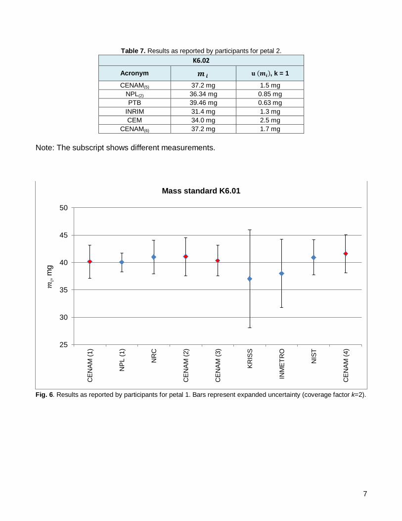
Table 7. Results as reported by participants for petal 2.
K6.02
Acronym 𝒎 𝒊 𝐮 (𝒎𝒊), k = 1
CENAM(5) 37.2 mg 1.5 mg
NPL(2) 36.34 mg 0.85 mg
PTB 39.46 mg 0.63 mg
INRIM 31.4 mg 1.3 mg
CEM 34.0 mg 2.5 mg
CENAM(6) 37.2 mg 1.7 mg
Note: The subscript shows different measurements.
Fig. 6. Results as reported by participants for petal 1. Bars represent expanded uncertainty (coverage factor k=2).
25
30
35
40
45
50
CE
NA
M (
1)
NP
L (
1)
NR
C
CE
NA
M (
2)
CE
NA
M (
3)
KR
ISS
INM
ET
RO
NIS
T
CE
NA
M (
4)
𝑚𝑖, m
g
Mass standard K6.01

8
Fig. 7. Results as reported by participants for petal 2. Bars represent expanded uncertainty (coverage factor k=2).
7. ANALYSIS OF RESULTS In order to link results of participants of both petals, the differences between results reported
by participants and pilot laboratory (𝑑𝑖𝑓𝑓𝑚 𝑖,𝑃𝐿) were calculated as follows,
𝑑𝑖𝑓𝑓𝑚 𝑖,𝑃𝐿 = 𝑚 𝑖 − 𝑚𝑃𝐿 − 𝜀𝑑𝑟𝑖𝑓𝑡 − 𝜀𝑟𝑒𝑝𝑟𝑜𝑑 (2)
with
𝑚𝑃𝐿 =𝑚𝑃𝐿 𝑖+𝑚𝑃𝐿 𝑖+1
2 (3)
where
𝑚𝑃𝐿 is the mean value of the results of the pilot laboratory measurements closest in
time to the measurement of participant i
𝑚𝑃𝐿 𝑖 is value reported by pilot laboratory before the measurement of participant i 𝑚𝑃𝐿 𝑖+1 is the value reported by pilot laboratory after the measurement of participant i 𝜀𝑑𝑟𝑖𝑓𝑡 is an error due to the possible drift of the travelling standards,
𝜀𝑟𝑒𝑝𝑟𝑜𝑑 is an error due to the reproducibility of the pilot laboratory,
25
30
35
40
45
50
CE
NA
M (
5)
NP
L (
2)
PT
B
INR
IM
CE
M
CE
NA
M (
6)
𝑚𝑖, m
g
Mass standard K6.02

9
The error due to the possible drift of the travelling standards, was estimated by the difference
between the measurements of the pilot laboratory before sending the travelling standard and
on its returns. The largest of the three possible values of this drift was taken as representative
for all participants. This drift error was considered as centred in zero with a uniform probability
density function (pdf) associated to this error.
Both, the expectation and the dispersion for the drift error (of the travelling standards) were
assumed as follows,
𝐸(𝜀𝑑𝑟𝑖𝑓𝑡) = 0 mg and 𝜎(𝜀𝑑𝑟𝑖𝑓𝑡 ) =𝑚𝑃𝐿 𝑖+1−𝑚𝑃𝐿 𝑖
√12 = 0.37 mg
As both pilot and co-pilot laboratories measured the two travelling standards, the error due to
the reproducibility associated to the measurements of the pilot laboratory was estimated by the
difference between its results and results reported by co-pilot laboratory for each petal,
(𝑑𝑖𝑓𝑓𝑚 𝑃𝐿−𝐶𝑜𝑃𝐿). A uniform pdf was considered associated to this error but centred in zero.
Both, the expectation and the dispersion for the reproducibility error (of the pilot laboratory)
were assumed as follows,
𝐸(𝜀𝑟𝑒𝑝𝑟𝑜𝑑) = 0 mg, and 𝜎(𝜀𝑟𝑒𝑝𝑟𝑜𝑑) =𝑑𝑖𝑓𝑓𝑚1 𝑃𝐿−𝐶𝑜𝑃𝐿−𝑑𝑖𝑓𝑓𝑚2 𝑃𝐿−𝐶𝑜𝑃𝐿
√12= 0.072 mg
7.1 Calculations of the Reference Value (RV), the mass differences between RV and participant laboratories, and the mass differences between any pair of participant laboratories
The median of the mass differences between results reported by participant and results
reported by pilot laboratory was calculated as the reference value for this key comparison,
𝑚𝑅𝑉.
𝑚𝑅𝑉 = 𝑚𝑒𝑑𝑖𝑎𝑛{𝑑𝑖𝑓𝑓𝑚 𝑖,𝑃𝐿; all reported values for all NMIs} (4)
The differences between mass reported by the participant laboratories and the reference value
were calculated as follows,
𝐷 𝑖 = 𝑑𝑖𝑓𝑓𝑚𝑖,𝑃𝐿 − 𝑚𝑅𝑉 (5)
In order to calculate the degree of equivalence for any pair of participant laboratories, the mass
differences between two laboratories, were calculated as follows,
𝑑 𝑖,𝑗 = 𝑑𝑖𝑓𝑓𝑚𝑖,𝑃𝐿 − 𝑑𝑖𝑓𝑓𝑚𝑗,𝑃𝐿 (6)

10
7.2 Numerical simulation by Monte Carlo method
In order to estimate the reference value for this key comparison (𝑚𝑅𝑉), the mass differences
between participants and reference value (𝐷 𝑖), and the mass differences between any pair of
participating laboratories (𝑑 𝑖,𝑗), a numerical simulation by Monte Carlo method was done.
The input quantities for the numerical simulation are listed in table 8. As the pilot and co-pilot
laboratories measured the two travelling standards, and even the pilot measured more than
once each travelling standard, the same correlation value between the measurements done by
the same laboratory was considered.
The correlation coefficient between mass measurements done by the same laboratory was
considered as 0.3 for any pair of them,
𝑟(𝑚𝐶𝐸𝑁𝐴𝑀 𝑖 , 𝑚𝐶𝐸𝑁𝐴𝑀 𝑗) = 0.3, 𝑟(𝑚𝑁𝑃𝐿 1 , 𝑚𝑁𝑃𝐿 2) = 0.3
The correlation coefficient indicated above, was estimated as 0.3 due to the variance
contribution of uncertainty type B is around 30 % with regard to the variance of the travelling
standard estimated by both pilot and co-pilot laboratories.
The mathematical models used for the numerical simulation were the corresponding to the eq.
2, 3, 4, 5 and 6.
From the resulting pdfs of the numerical simulation, the mean values were taken as the best
estimated for the corresponding differences, and the standard deviations were taken as the
standard uncertainty of such differences.
The numerical simulation was done in @Risk for Microsoft Excel 5.5 with 1×10⁵ trials. Results
of numerical simulation were confirmed by conducting an independent simulation with R
software. Differences between results of these two software tools are negligible.
The output quantities of the numerical simulation are listed in tables from 9 to 11, and some
resulting histograms of the outputs quantities are shown in Fig. 8, and from Fig. 10 to Fig. 18.
Fig. 9 is a graphical representation of the degree of equivalence between results reported by
laboratories and the reference value of this key comparison.

11
7.3 Input quantities for the numerical simulation In the next table are listed the input quantities for the numerical simulation.
Table 8. Input quantities for the numerical simulation.
Xi Distribution
Parameters
Expectation
Standard deviation
Expectation
𝒙 = (𝒂 + 𝒃) 𝟐⁄
Semi-width
(𝒂 − 𝒃) 𝟐⁄
𝑚𝐶𝐸𝑁𝐴𝑀 1 𝑁(𝜇, 𝜎2) 4.2 mg 1.5 mg
𝑚𝑁𝑃𝐿 1 𝑁(𝜇, 𝜎2) 40.03 mg 0.85 mg
𝑚𝑁𝑅𝐶 𝑁(𝜇, 𝜎2) 41.0 mg 1.5 mg
𝑚𝐶𝐸𝑁𝐴𝑀 2 𝑁(𝜇, 𝜎2) 41.1 mg 1.7 mg
𝑚𝐶𝐸𝑁𝐴𝑀 3 𝑁(𝜇, 𝜎2) 40.3 mg 1.3 mg
𝑚𝐾𝑅𝐼𝑆𝑆 𝑁(𝜇, 𝜎2) 37.0 mg 4.5 mg
𝑚𝐼𝑁𝑀𝐸𝑇𝑅𝑂 𝑁(𝜇, 𝜎2) 38.0 mg 3.1 mg
𝑚𝑁𝐼𝑆𝑇 𝑁(𝜇, 𝜎2) 40.9 mg 1.6 mg
𝑚𝐶𝐸𝑁𝐴𝑀 4 𝑁(𝜇, 𝜎2) 41.6 mg 1.7 mg
𝑚𝐶𝐸𝑁𝐴𝑀5 𝑁(𝜇, 𝜎2) 37.2 mg 1.5 mg
𝑚𝑁𝑃𝐿 2 𝑁(𝜇, 𝜎2) 36.34 mg 0.85 mg
𝑚𝑃𝑇𝐵 𝑁(𝜇, 𝜎2) 39.46 mg 0.63 mg
𝑚𝐼𝑁𝑅𝐼𝑀 𝑁(𝜇, 𝜎2) 31.4 mg 1.3 mg
𝑚𝐶𝐸𝑀 𝑁(𝜇, 𝜎2) 34.0 mg 2.5 mg
𝑚𝐶𝐸𝑁𝐴𝑀 6 𝑁(𝜇, 𝜎2) 37.2 mg 1.7 mg
𝜀𝑑𝑟𝑖𝑓𝑡 𝑈(𝑎, 𝑏) 0.00 mg 0.65 mg
𝜀𝑟𝑒𝑝𝑟𝑜𝑑 𝑈(𝑎, 𝑏) 0.00 mg 0.14 mg
Note:
𝑁(𝜇, 𝜎2) Normal distribution 𝑈(𝑎, 𝑏) Uniform distribution

12
7.4 Output quantities of the numerical simulation Results of numerical simulation are shown in 7.4.1 and 7.4.2. The mean values of the pdfs, resulting from the numerical simulation, were taken as the best estimates of the output quantities and the standard deviations as the corresponding standard uncertainties. In order to avoid losing useful information, simulation results are reported with two decimal digits, (not necessarily two significant digits). 7.4.1 Reference value 𝒎𝑹𝑽, and degree of equivalence between NMIs and the reference value 𝑫 𝒊
The key comparison reference value and its dispersion are shown in table 9. The histogram resulting from the numerical simulation is shown in Fig. 8. In table 10, are listed the degree of equivalence between participant laboratories and reference value and their uncertainties. The confidence intervals of 𝐷 𝑖 to 95% resulting from numerical simulation are also shown in table 10. In
Fig. 9 are shown the resulting 𝐷 𝑖; uncertainty bars are shown with 𝑘 = 2. The normalized errors calculated for each 𝐷 𝑖 also are listed in table 10. Table 9. Data of the median resulting of numerical simulation.
𝒎𝑹𝑽, mg -0.90
𝒖(𝒎𝑹𝑽), mg 1.20
𝑼(𝒎𝑹𝑽), 𝒌 = 𝟐, mg 2.40
P[x1, x2] 95%, mg [-3.52, 1.15]
Fig. 8. Histogram resulting from simulation corresponding to the KCRV. Values are in milligrams.

13
Table 10. Mass differences between participant laboratories and Reference Value, 𝐷 𝑖 .
CENAM PTB KRISS NPL NRC NIST INMETRO INRIM CEM
𝐷𝑖, mg 0.90 3.17 -3.06 0.17 1.27 0.84 -2.06 -4.89 -2.34
𝑢(𝐷𝑖), mg 1.14 1.30 4.39 1.00 1.69 1.68 3.06 1.73 2.57
𝑈(𝐷𝑖), 𝑘 = 2, mg 2.28 2.60 8.78 2.00 3.38 3.36 6.12 3.46 5.14
P[x1, x2] 95%, mg [-1.06, 3.44] [0.63, 5.82] [-11.99, 5.40] [-1.90, 2.45] [-1.83, 4.90] [-2.47, 4.45] [-8.30, 3.80] [-8.26, -1.45] [-7.64, 2.44]
𝐸𝑛 = |𝐷𝑖| 𝑈(𝐷𝑖)⁄ 0.39 1.22 0.35 0.09 0.38 0.25 0.34 1.41 0.46
Fig. 9. Mass differences between results reported by participant laboratories and the reference value, 𝐷 𝑖. The uncertainty bars are shown with a
coverage factor 𝑘 = 2.
-14.00
-12.00
-10.00
-8.00
-6.00
-4.00
-2.00
0.00
2.00
4.00
6.00
8.00
CENAM PTB KRISS NPL NRC NIST INMETRO INRIM CEM
Di,
in m
illig
ram
s

14
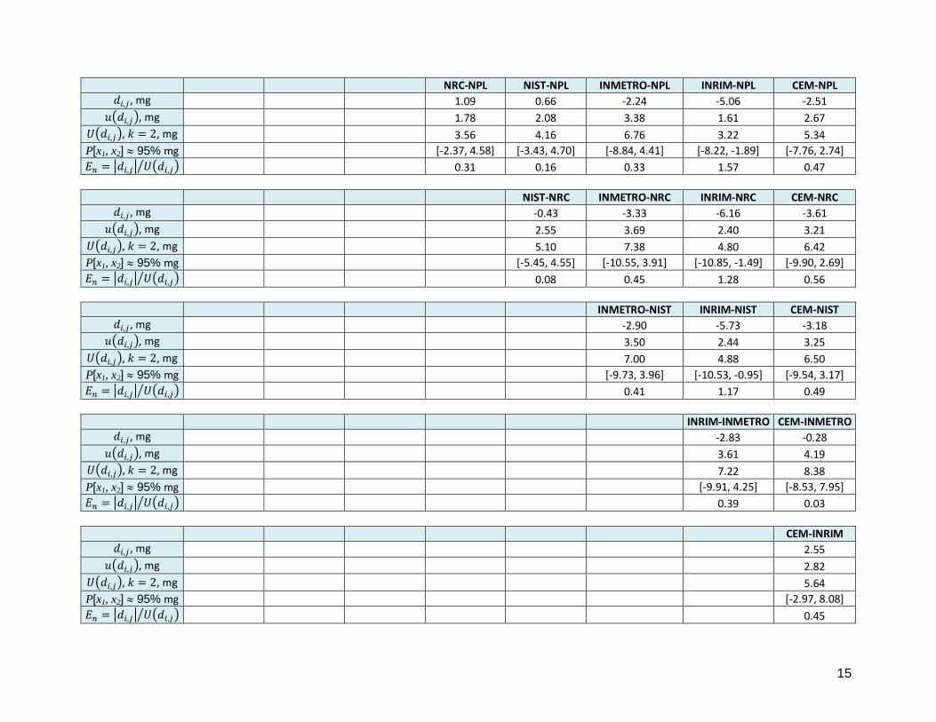
7.4.2 Degree of equivalence between any pair of NMIs, 𝒅 𝒊,𝒋
Even when the mass difference between any pair of participant laboratories (degree of equivalence) is no longer required for publishing on KCDB, see [10], in this report these values are presented as additional information. The mass differences between any pair of NMIs were calculated in the numerical simulations as well as the corresponding uncertainties; all these values are listed in table 11. These mass differences are taken as the degrees of equivalence
between pairs of NMIs (𝑑 𝑖,𝑗). The uncertainty 𝑢( 𝑑 𝑖,𝑗), and the confidence intervals of each 𝑑 𝑖,𝑗 to 95% resulting from
numerical simulation and the normalized errors 𝐸𝑛 calculated for each 𝑑 𝑖,𝑗 are also shown in table 11.
In annex A, are shown the histograms of degrees of equivalence resulting from numerical simulation.
Table 11. Mass differences between any pair of participant laboratories, 𝑑𝑖,𝑗
PTB-CENAM KRISS-CENAM NPL-CENAM NRC-CENAM NIST-CENAM INMETRO-CENAM INRIM-CENAM CEM-CENAM
𝑑𝑖,𝑗 , mg 2.27 -3.96 -0.73 0.36 -0.07 -2.97 -5.79 -3.24
𝑢(𝑑𝑖,𝑗), mg 1.44 4.66 1.30 1.98 2.01 3.33 1.83 2.81
𝑈(𝑑𝑖,𝑗), 𝑘 = 2, mg 2.88 9.32 2.60 3.96 4.02 6.66 3.66 5.62
P[x1, x2] 95% mg [-0.55, 5.09] [-13.10, 5.19] [-3.27, 1.82] [-3.52, 4.25] [-4.02, 3.87] [-9.50, 3.60] [-9.38, -2.21] [-8.77, 2.27]
𝐸𝑛 = |𝑑𝑖,𝑗| 𝑈(𝑑𝑖,𝑗)⁄ 0.79 0.42 0.28 0.09 0.02 0.45 1.58 0.58
KRISS-PTB NPL-PTB NRC-PTB NIST-PTB INMETRO-PTB INRIM-PTB CEM-PTB
𝑑𝑖,𝑗 , mg
-6.23 -3.00 -1.90 -2.33 -5.23 -8.06 -5.51
𝑢(𝑑𝑖,𝑗), mg
4.72 1.14 2.10 2.17 3.43 1.44 2.57
𝑈(𝑑𝑖,𝑗), 𝑘 = 2, mg
9.44 2.28 4.2 4.34 6.86 2.88 5.14
P[x1, x2] 95% mg
[-15.52, 3.00] [-5.24, -0.75] [-6.02, 2.23] [-6.60, 1.89] [-11.91, 1.51] [-10.89, -5.23] [-10.55, -0.47]
𝐸𝑛 = |𝑑𝑖,𝑗| 𝑈(𝑑𝑖,𝑗)⁄
0.66 1.32 0.45 0.54 0.76 2.80 1.07
NPL-KRISS NRC-KRISS NIST-KRISS INMETRO-KRISS INRIM-KRISS CEM-KRISS
𝑑𝑖,𝑗 , mg
3.23 4.33 3.90 1.00 -1.83 0.72
𝑢(𝑑𝑖,𝑗), mg
4.68 4.92 4.78 5.46 4.86 5.31
𝑈(𝑑𝑖,𝑗), 𝑘 = 2, mg
9.36 9.84 9.56 10.92 9.72 10.62
P[x1, x2] 95% mg
[-5.90, 12.46] [-5.34, 13.99] [-5.39, 13.27] [-9.76, 11.72] [-11.33, 7.70] [-9.65, 11.17]
𝐸𝑛 = |𝑑𝑖,𝑗| 𝑈(𝑑𝑖,𝑗)⁄
0.35 0.44 0.41 0.09 0.20 0.07
15
NRC-NPL NIST-NPL INMETRO-NPL INRIM-NPL CEM-NPL
𝑑𝑖,𝑗 , mg
1.09 0.66 -2.24 -5.06 -2.51
𝑢(𝑑𝑖,𝑗), mg
1.78 2.08 3.38 1.61 2.67
𝑈(𝑑𝑖,𝑗), 𝑘 = 2, mg
3.56 4.16 6.76 3.22 5.34
P[x1, x2] 95% mg
[-2.37, 4.58] [-3.43, 4.70] [-8.84, 4.41] [-8.22, -1.89] [-7.76, 2.74]
𝐸𝑛 = |𝑑𝑖,𝑗| 𝑈(𝑑𝑖,𝑗)⁄
0.31 0.16 0.33 1.57 0.47
NIST-NRC INMETRO-NRC INRIM-NRC CEM-NRC
𝑑𝑖,𝑗 , mg
-0.43 -3.33 -6.16 -3.61
𝑢(𝑑𝑖,𝑗), mg
2.55 3.69 2.40 3.21
𝑈(𝑑𝑖,𝑗), 𝑘 = 2, mg
5.10 7.38 4.80 6.42
P[x1, x2] 95% mg
[-5.45, 4.55] [-10.55, 3.91] [-10.85, -1.49] [-9.90, 2.69]
𝐸𝑛 = |𝑑𝑖,𝑗| 𝑈(𝑑𝑖,𝑗)⁄ 0.08 0.45 1.28 0.56
INMETRO-NIST INRIM-NIST CEM-NIST
𝑑𝑖,𝑗 , mg
-2.90 -5.73 -3.18
𝑢(𝑑𝑖,𝑗), mg
3.50 2.44 3.25
𝑈(𝑑𝑖,𝑗), 𝑘 = 2, mg
7.00 4.88 6.50
P[x1, x2] 95% mg
[-9.73, 3.96] [-10.53, -0.95] [-9.54, 3.17]
𝐸𝑛 = |𝑑𝑖,𝑗| 𝑈(𝑑𝑖,𝑗)⁄
0.41 1.17 0.49
INRIM-INMETRO CEM-INMETRO
𝑑𝑖,𝑗 , mg
-2.83 -0.28
𝑢(𝑑𝑖,𝑗), mg
3.61 4.19
𝑈(𝑑𝑖,𝑗), 𝑘 = 2, mg
7.22 8.38
P[x1, x2] 95% mg
[-9.91, 4.25] [-8.53, 7.95]
𝐸𝑛 = |𝑑𝑖,𝑗| 𝑈(𝑑𝑖,𝑗)⁄
0.39 0.03
CEM-INRIM
𝑑𝑖,𝑗 , mg
2.55
𝑢(𝑑𝑖,𝑗), mg
2.82
𝑈(𝑑𝑖,𝑗), 𝑘 = 2, mg
5.64
P[x1, x2] 95% mg
[-2.97, 8.08]
𝐸𝑛 = |𝑑𝑖,𝑗| 𝑈(𝑑𝑖,𝑗)⁄ 0.45

16
8. SUMMARY AND CONCLUSIONS
The report summarizes the procedure and results of CCM.M-K6, a key comparison of 50 kg weights. For this key comparison nine National Metrology Institutes (NMIs) took part. The NMIs belong to the following Regional Metrology Organizations: SIM (4), EURAMET (4) and APAP (1). Two mass standards made of stainless steel and characterized at the pilot laboratory were circulated in two petals from April of 2011 to June of 2013. Both travelling standards were measured by the pilot laboratory at the beginning and at the end of the circulation in order to monitor the drift of the travelling standards. The co-pilot laboratory measured both travelling standards after the first measurement of the pilot laboratory. The traveling standard K6.01 was additionally measured by the pilot laboratory in the middle of the circulation, this measurement was done for control due to the time elapsed between the transfer of the weight between NRC and KRISS (see table 4). Both travelling standards show good stability and, no significant drift was found in the control measurements, however uncertainty contributions due to the drift and repeatability of the pilot laboratory measurements were estimated and considered in the calculations. The median of the mass difference between results reported by participant laboratories and pilot laboratory was taken as the key comparison reference value (KCRV, see Chap. 7.4.1). Degrees of equivalence between results reported by NMIs and key comparison reference value were calculated and reported in table 10. For two of the nine laboratories, INRIM and PTB, the difference from the key comparison reference value exceeds the expanded uncertainty in the difference (see table 10). Degrees of equivalence between results of pairs of NMIs were calculated and reported in table 11. In order to validate the calculation of the degrees of equivalence between results of NMIs and KCRV and alternative analysis was performed (Olha Bodnar, Clemens Elster, PTB see Annex B); no significant differences were found between the values calculated by the two methods. Note: The weighted mean of the deviations of the results of the laboratories, which have recalibrated their prototypes more than five years before the comparison, i.e. before 2008, to the BIPM is about -0,016 mg at the kilogram level (CCM.M-K4 [9]). This corresponds to a shift of -0,8 mg at the 50 kg level which could potentially affect the results of this comparison.

17
REFERENCES
[1] Consultative Committee for Mass and Related Quantities (CCM), Report of the 13th meeting. 12 -13 May, 2011. BIPM, Sèvres France.
[2] JCGM 100:2008, Evaluation of measurement data – Guide to the expression of the uncertainty in measurements.
[3] JCGM 101:2008, Evaluation of the measurement data – Supplement 1 to the “Guide to the expression of the uncertainty in measurements” – Propagation of distributions using a Monte Carlo Method.
[4] JCGM 102:2011, Evaluation of the measurement data – Supplement 2 to the “Guide to the expression of the uncertainty in measurements” – Extension to any number of output quantities.
[5] R Core Team (2013). R: A language and environment for statistical computing. R Foundation for Statistical Computing, Vienna, Austria. URL http://www.R-project.org/.
[6] McKay, M.D., Conover, W.J., and Beckman, R.J. (1979). “A Comparison of Three Methods for Selecting Values of Input Variables in the Analysis of Output from a Computer Code,” Technometrics, 221, 239-245.
[7] Toman, B., and Possolo, A. (2009). “Laboratory Effects Models for Interlaboratory Comparisons,” Accreditation and Quality Assurance, 14, 553-563.
[8] Bodnar, O., Link, A., and Elster, C. (2014). “Bayesian Treatment of a Random Effects Model for the Analysis of Key Comparisons,” MATHMET 2014, Berlin, 24-26 March 2014.
[9] Luis Omar Becerra et al. (2014). Final report on CCM.M-K4: Key comparison of 1 kg stainless steel mass standards. Metrologia 51 07009
[10] CCM-WGS. CCM Guidelines for the approval and publication of the final reports of key and supplementary comparison, 29 August 2013.
ACKNOWLEDGEMENTS
The authors would like to acknowledge the kind assistance of all colleagues in the participating laboratories for helping this comparison.
Luis Manuel Peña, CENAM
Luis Manuel Ramírez, CENAM
Hugo Gasca, CENAM
Manuel Bautista, CEM
Francisco Javier Gamarra, CEM
Jin Wan Chung, KRISS
Fábio André Ludolf Cacais, INMETRO
Anderson Beatrici, INMETRO
Arlindo dos Santos Rebelo Junior, INMETRO
Michael Mecke, PTB
Thomas Tippelt, PTB
Olha Bodnar, PTB
Clemens Elster, PTB
Zeina J. Kubarych, NIST
Antonio Possolo, NIST

18
ANNEX A Histograms resulting from numerical simulation for degrees of equivalence between NMIs and Reference Value, 𝐷𝑖, Fig. 10 – 18.

19
Fig. 10. Histogram resulting for 𝐷𝐶𝐸𝑁𝐴𝑀
Fig. 11. Histogram resulting for 𝐷𝑃𝑇𝐵
Fig. 12. Histogram resulting for 𝐷𝐾𝑅𝐼𝑆𝑆

20
Fig. 13. Histogram resulting for 𝐷𝑁𝑃𝐿
Fig. 14. Histogram resulting for 𝐷𝑁𝑅𝐶
Fig. 15. Histogram resulting for 𝐷𝑁𝐼𝑆𝑇

21
Fig. 16. Histogram resulting for 𝐷𝐼𝑁𝑀𝐸𝑇𝑅𝑂
Fig. 17. Histogram resulting for 𝐷𝐼𝑁𝑅𝐼𝑀
Fig. 18. Histogram resulting for 𝐷𝐶𝐸𝑀

22
ANNEX B Alternative analysis of results
In the following, results of an alternative analysis method are presented. The alternative
method is based on random effects models [7, 8] and uses different (statistical) assumptions
than the median-based method applied in this report. Nonetheless, the alternative method
arrives at the same conclusions, which can be seen as a confirmation of the reported results.
As regards the general application of random effects models for the analysis to KCs we refer to
[7].
The alternative method has several advantages. It is based on a statistical model which allows
for a treatment of the original data quoted by the laboratories. This is in contrast to the median-
based method which first constructs differences of the results to a single laboratory (the pilot in
this case). As a consequence, the alternative method does not treat the pilot laboratory in a
special way as does the median-based method. Furthermore, no correlations are introduced as
for the median-based method (through the construction of differences to the same single lab),
and Monte Carlo simulations are also not required.
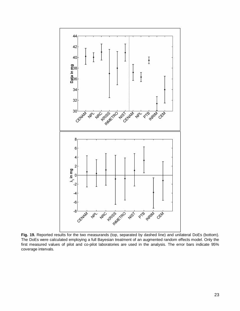
In order to analyse the data (see Fig. 19, top) in a way that does not treat the pilot laboratory
differently than the remaining laboratories, the subsequent model was applied,
XXXελ1X ,
YYYελ1Y ,
where the vectors T
XX ),,(61
X and T
YY ),,(51
Y refer to the measurement
results for petal 1 and petal 2, respectively, X denotes the (unknown) weight of petal 1, and
Y that of petal 2. The errors X
ε and Yε are assumed to be normally (and independently)
distributed with zero means and variances equal to the squares of the quoted standard
uncertainties. The vectors YXλλ , are the so-called random effects which are assumed to be
distributed according to ),(~,2I0λλ
YXN with
pilotpilotYX
λλ and pilotcopilotco
YX
λλ . (In
the analysis only the first measurement result of the pilot laboratory was used for each of the
two petals, and the co-pilot laboratory was treated similarly.)
The subsequent results were obtained by applying a full Bayesian treatment of the above
model using appropriate non-informative priors [8]. For the unilateral DoEs, the resulting
estimates of the i
, together with their 95% (probabilistically symmetric) credible intervals, are
taken. (Since these credible intervals are in general not symmetric around the estimate, we do
not state an expanded uncertainty, and hence also not an En number). Fig. 19 shows the
according results, which are in a remarkable agreement with those obtained by the median-
based method.
23
Fig. 19. Reported results for the two measurands (top, separated by dashed line) and unilateral DoEs (bottom).
The DoEs were calculated employing a full Bayesian treatment of an augmented random effects model. Only the
first measured values of pilot and co-pilot laboratories are used in the analysis. The error bars indicate 95%
coverage intervals.

24
Table 12. DoEs i
.
CENAM PTB KRISS NPL NRC NIST INMETRO INRIM CEM
i in mg 0.75 3.29 -0.85 0.38 1.16 1.06 -0.76 -3.83 -1.19
𝑢 (i
) in mg 1.74 1.44 2.69 1.49 1.76 1.80 2.35 1.67 2.15
95% coverage interval in mg
[-2.62, 4.32]
[0.53, 6.30]
[-6.50, 4.43]
[-2.54, 3.45]
[-2.24, 4.81]
[-2.43, 4.79]
[-5.55, 3.84]
[-7.35, -0.58]
[-5.61, 3.02]


![Product overview Termination Carrier [PDF, 0.22 MB]](https://img.pdfslide.net/doc/110x75/5867d8b31a28ab87408bdc71/product-overview-termination-carrier-pdf-022-mb.jpg)

