Embed Size (px)
Citation preview
FINAL REPORT
Residential Nonparticipant
Customer Profile Study MA19X06-B-RESNONPART
Date: February 6, 2020

DNV GL – www.dnvgl.com February 6, 2020 Page i
Table of contents
1 EXECUTIVE SUMMARY ..................................................................................................... 1
1.1 Study purpose and objectives 1
1.2 Key findings, implications, recommendations, and considerations 3 1.2.1 Comparison to the Market Barriers Study 6
1.3 Methodology overview 8 1.3.1 Provisions 9
2 INTRODUCTION ............................................................................................................ 12
2.1 Study purpose, objectives, and research questions 12
2.2 Organization of report 14
3 METHODOLOGY AND APPROACH ..................................................................................... 15
3.1 Participation by block group list preparation 15
3.2 Participant-Nonparticipant list preparation 15 3.2.1 Renter flag 17 3.2.2 Modeling 21
3.3 Hot spot analysis 27
4 ANALYSIS AND RESULTS ............................................................................................... 28
4.1 ACS variable correlations 28 4.1.1 Hot spot analysis 30
4.2 Electric location participation findings 31 4.2.1 ACS variable correlations with electric participation 31 4.2.2 Electric participation block group-level models 34 4.2.3 Electric participation individual-level models 36
4.3 Electric savings/consumption findings 41 4.3.1 Block group electric analysis 41 4.3.2 Individual-level electric analysis – Statewide 45 4.3.3 Individual-level electric analysis – Enhanced 46 4.3.4 Location participation and savings/consumption inconsistencies 47
4.4 Gas location participation findings 50 4.4.1 ACS variable correlations with gas participation 50 4.4.2 Gas participation block group-level models 51 4.4.3 Gas participation individual-level models 56
4.5 Gas savings/consumption findings 60 4.5.1 Block group gas analysis 60 4.5.2 Individual-level gas analysis – Statewide 63 4.5.3 Individual-level gas analysis – Enhanced 64 4.5.4 Location participation and savings/consumption inconsistencies 66
5 CONCLUSIONS, RECOMMENDATIONS, AND CONSIDERATIONS ........................................... 69
5.1 Conclusions 69 5.1.1 Location participation rates for 2013-2017 are negatively associated with all three
term sheet variables: moderate-income households, renter households, and limited
English-speaking households. 69 5.1.2 PA efforts to obtain participation from large multifamily locations have resulted in
some inclusion of the populations outlined in the term sheet. 69 5.1.3 When participation is measured using 2013-2017 savings/consumption, it is positively
correlated with low income and multifamily at the block group level. 69 5.1.4 Location participation rates for 2013-2017 are affected by multiple factors. 69

DNV GL – www.dnvgl.com February 6, 2020 Page ii
5.1.5 Most of the variables investigated are correlated with each other, especially in the ACS data. 69
5.1.6 Term sheet-related populations are geographically clustered in urban areas. 70 5.1.7 Limited-English speakers are more likely to rent, and renters are less likely to
participate. 70 5.1.8 The effects of the examined variables on participation are similar in both electric and
gas markets. 70 5.1.9 The individual-level models are mostly consistent with the block group-level models. 70 5.1.10 Comparison to the Market Barriers Study 70
5.2 Recommendations 73
5.3 Considerations 74
6 APPENDIX A: PARTICIPANT/NONPARTICIPANT LIST PREPARATION ..................................... 75
7 APPENDIX B: LOW PARTICIPATION TABLE ....................................................................... 86
8 APPENDIX C: BIVARIATE MAPS .................................................................................... 122
9 APPENDIX D: CLOSE-UP HOTSPOT MAPS ....................................................................... 135
List of figures Figure 3-1. Renter flag definition ...................................................................................................... 19 Figure 4-1. Statewide ACS variable hot spot map, subset to urbanized land areas only ............................ 30 Figure 4-2. Block group-level electric participation correlations (term sheet variables) ............................. 32 Figure 4-3. Block group-level electric participation correlations (extra ACS variables) .............................. 33 Figure 4-4. Renter*Multifamily interaction on electric account participation probability – statewide ........... 38 Figure 4-5. Renter*Limited English interaction on electric account participation probability – enhanced data .................................................................................................................................................... 40 Figure 4-6. Renter*Multifamily interaction on electric account participation probability – enhanced data .... 41 Figure 4-7. Block group electric correlations ....................................................................................... 42 Figure 4-8. Multifamily interactions with low income and renter ............................................................ 44 Figure 4-9. Individual-level correlations with savings over consumption, statewide electric ...................... 45 Figure 4-10. Individual-level correlations with savings over consumption, enhanced electric .................... 46 Figure 4-11. Block group correlations, electric, no LIMF savings ............................................................ 49 Figure 4-12. Block group-level gas participation correlations (term sheet variables) ................................ 50 Figure 4-13. Block group-level gas participation correlations (extra ACS variables) ................................. 51 Figure 4-14. Expected gas location participation rate (renter * multifamily) ........................................... 55 Figure 4-15. Renter* multifamily interaction on gas account participation probability – statewide ............. 58 Figure 4-16. Renter* multifamily interaction on gas account participation probability – enhanced data ...... 60 Figure 4-17. Block group gas correlations .......................................................................................... 61 Figure 4-18. Interaction of low income and multifamily on gas savings/consumption ............................... 63 Figure 4-19. Interaction of rent and multifamily on gas savings/consumption ......................................... 63 Figure 4-20. Individual-level correlations with savings over consumption, statewide gas .......................... 64 Figure 4-21. Individual-level correlations with savings over consumption, enhanced gas .......................... 65 Figure 4-22. Block group correlations, gas, no LIMF savings ................................................................. 68 Figure 7-1. Community Outreach Metric formula and features .............................................................. 86 Figure 9-1. ACS variable hot spot map, closeup of Worcester and surrounding areas ............................. 136 Figure 9-2. ACS variable hot spot map, closeup of Springfield, Holyoke, and surrounding areas .............. 137 Figure 9-3. ACS variable hot spot map, closeup of Lawrence and surrounding areas .............................. 138 Figure 9-4. ACS variable hot spot map, closeup of Fitchburg and surrounding areas .............................. 139 Figure 9-5. ACS variable hot spot map, closeup of Fall River and surrounding areas .............................. 140 Figure 9-6. ACS variable hot spot map, closeup of Boston and surrounding areas ................................. 141
DNV GL – www.dnvgl.com February 6, 2020 Page iii
List of tables Table 1-1. Key findings of residential nonparticipant studies ................................................................... 6 Table 3-1. Final record counts by fuel and PA ..................................................................................... 16 Table 3-2. Number of electric accounts per location, 2014-2017 ........................................................... 18 Table 3-3. Number of gas accounts per location, 2014-2017 ................................................................ 18 Table 3-4. Number of accounts per location for Experian’s likely renters not flagged as a condo location.... 19 Table 3-5. Experian renter flag location comparison ............................................................................ 19 Table 3-6. Electric PA renter summary ............................................................................................... 20 Table 3-7. Gas PA renter summary ................................................................................................... 20 Table 3-8. PNP renter flag block group comparison with ACS block group percent renter.......................... 21 Table 4-1. ACS variable correlations .................................................................................................. 28 Table 4-2. Initial electric block group models ...................................................................................... 34 Table 4-3. Electric location participation models with some variables removed ........................................ 35 Table 4-4. Electric consumption weighted location participation models renter variable present/absent ..... 35 Table 4-5. Electric block group model results with all variables ............................................................. 36 Table 4-6. Individual-level correlations – statewide electric .................................................................. 37 Table 4-7. Electric account participation models coefficients – statewide ................................................ 38 Table 4-8. Individual-level correlations – Enhanced electric data ........................................................... 39 Table 4-9. Electric account participation models coefficients – enhanced data ......................................... 40 Table 4-10. Electric savings/consumption model results, block group-level ............................................. 43 Table 4-11. Individual-level savings over consumption models, statewide electric ................................... 45 Table 4-12. Individual-level savings over consumption models, enhanced electric ................................... 47 Table 4-13. Block group participation models comparison, electric ........................................................ 47 Table 4-14. Savings/consumption models, aggregated account-level data, electric .................................. 48 Table 4-15. Initial gas block group models ......................................................................................... 52 Table 4-16. Gas location participation models; renter variable present/absent ........................................ 53 Table 4-17. Gas consumption weighted location participation models renter variable present/absent ......... 53 Table 4-18. Gas block group model results with all variables ................................................................ 55 Table 4-19. Individual-level correlations – Statewide Gas..................................................................... 56 Table 4-20. Gas account participation models coefficients – statewide ................................................... 57 Table 4-21. Individual-level correlations – Enhanced Gas data .............................................................. 58 Table 4-22. Gas account participation models coefficients – enhanced data ............................................ 59 Table 4-23. Gas savings/consumption model results ........................................................................... 62 Table 4-24. Individual-level savings over consumption models, statewide gas ........................................ 64 Table 4-25. Individual-level savings over consumption models, enhanced gas ........................................ 66 Table 4-26. Block group participation models comparison, electric ........................................................ 66 Table 4-27. Savings/consumption models, aggregated account-level data, electric .................................. 67 Table 5-1. Key findings of residential nonparticipant studies ................................................................. 71 Table 6-1. Unique accounts in tracking data (Fuel*PA*year) ................................................................ 75 Table 6-2. Residential unique accounts by fuel and PA ......................................................................... 76 Table 6-3. C&I Unique accounts by fuel and PA (before removing nonresidential) ................................... 77 Table 6-4. Final record counts by fuel and PA ..................................................................................... 79 Table 7-1. Highest and lowest scoring town analysis ........................................................................... 88 Table 7-2. Community outreach metric table: Dual-fuel ....................................................................... 89 Table 7-3. Community outreach metric table: Gas .............................................................................. 99 Table 7-4. Community outreach metric table: Electric........................................................................ 109

DNV GL – www.dnvgl.com February 6, 2020 Page 1
1 EXECUTIVE SUMMARY
1.1 Study purpose and objectives
DNV GL conducted the Residential Nonparticipant Analysis Study (MA19X06-B-RESNONPART; “NPA”) for the
Massachusetts Program Administrators (PAs) and Energy Efficiency Advisory Council (EEAC) Consultants
from February 1, 2019, to December 20, 2019. The study’s overall purpose is to assess relationships
between residential participation rates and the variables specified in the PAs’ October 19, 2018 term sheet,
which stipulates:
“Special Focus on Renters, Moderate Income, Non-English Speaking, and Small Business Customers:
The Program Administrators will conduct tailored evaluations in 2019 that address participation
levels and potential unaddressed barriers for (a) businesses (small, medium and large) and (b)
residential customers by income levels and by non-English speaking populations (utilizing proxy
methods that do not rely on specific income or demographic information from Mass Save®
participants). The Program Administrators will leverage the existing EM&V framework, and present
full results of the studies to the EEAC.”1
This study was developed to provide information relevant to this term sheet stipulation. The study
objectives, as established by the working group, are as follows:
1. Quantify recent (2013-2017) levels of participation in PA programs for renters, moderate-income
customers, and non-English-speaking customers
2. Quantify how various factors (including but not limited to income level, language barriers, building
ownership, and single or multifamily) are associated with participation in Mass Save residential programs
3. Address the possibility of ecological fallacy2 when using block group-level variables
4. Establish a baseline level of participation that can be used to assess the effectiveness of PA efforts to
increase outreach
The main body of this report addresses the first 3 objectives. It presents the results of the tasks involving
statistical modeling to characterize the relationships between the term sheet variables, participation, and
other available demographic variables. The multiple levels of modeling also helped determine the extent of
ecological fallacy in the block group-level analyses. We also provide implications and recommendations
derived from these findings. Two additional, separate deliverables added to the information in this report:
• A “low participation” table that shows levels of the term sheet variables and location participation rates
by town and block group level. This deliverable addresses objectives 1 and 4. A copy of the town-level
data provided through this deliverable is included in Appendix B (Section 7) of this document.
• A series of bivariate maps that provide visualizations of areas with high concentrations of the term sheet
characteristics that have low participation rates. A copy of this deliverable is included in Appendix C of
this document.
This study provided a foundational analysis of participation patterns to identify underserved customers. This
analysis fed into a subsequent study called the “Residential Nonparticipant Market Characterization and
Barriers Study” (Market Barriers Study). The Market Barriers Study was a market assessment that
1 http://ma-eeac.org/wordpress/wp-content/uploads/Term-Sheet-10-19-18-Final.pdf
2 Ecological fallacy occurs when one makes conclusions about an individual based on group-level variables.

DNV GL – www.dnvgl.com February 6, 2020 Page 2
conducted primary research (including surveys and in-depth interviews) to explore market barriers for the
underserved customer segments, and to develop recommendations to more effectively reach those
segments.
This study is also related to the 2013-2017 Residential Customer Profile Study. Both reports have generally
consistent findings.

DNV GL – www.dnvgl.com February 6, 2020 Page 3
1.2 Key findings, implications, recommendations, and considerations
Study
Objective
Key finding Implication Consideration/Recommendations
1,2
Location participation rates for
2013-2017 are negatively
associated with all three term
sheet variables: moderate-
income households, renter
households, and limited English-
speaking households.
The populations represented by the
term sheet participate at lower levels
than other populations. This is not
surprising based on known barriers with
these populations.
Continue to explore program designs that will
help these populations overcome the
participation barriers they face.
1,2
Especially when participation is
measured as the ratio of 2013-
2017 savings to consumption,
there is evidence that the PAs
have had some success in
getting low-income and
multifamily (MF) locations to
participate.
The PAs’ success with low-income,
multifamily locations has enabled some
of the term sheet-related populations to
benefit from the programs because
multifamily is correlated with renters,
low-income, and limited English
speaking.
All PAs tracking participation at the individual
unit level would increase the accuracy of
evaluation results for MF buildings. For
implementers, knowing at a finer granularity
what they did in a building would help identify
opportunities to revisit buildings that have
participated in the past.
1,2
When participation is measured
using 2013-2017
savings/consumption, it is
positively correlated with low
income and multifamily at the
block group level. Additional
analysis revealed that savings
from the low income multifamily
programs account for these
positive correlations.
The PAs’ low income multifamily
programs are succeeding at achieving
depth of savings in areas with high
concentrations of low income
households and multifamily housing.
Future participation analyses should remain
aware of the strengths and limitations of each
way of measuring participation, and carefully
choose which definition to use in each analysis
based on the conceptual question being asked.
Consider whether the recently completed
multifamily study can answer any of the
outstanding questions, and consider
conducting a follow-up multifamily study to
further explore the outstanding questions.

DNV GL – www.dnvgl.com February 6, 2020 Page 4
Study
Objective
Key finding Implication Consideration/Recommendations
2
Location participation for 2013-
2017 is individually, negatively
correlated with the following
characteristics: low income and
pre-1950 construction and
individually; positively
correlated with average or
higher income and post-1950
construction.
Participation is affected by multiple
factors.
PAs could use this information for program
targeting.
2
Most of the variables
investigated are correlated with
each other, especially in the
ACS block group data.
Increasing participation among one of
the term sheet-related populations is
likely to also increase participation
among the other term sheet-related
populations.
Use the bivariate maps provided in this study
and other methods of identifying geospatial
areas to target program outreach efforts. The
bivariate maps provide a way to identify the
block groups that are the greatest outliers in
terms of the high incidence of term sheet
variables and low participation rates.
2
Term sheet-related populations
are geographically clustered in
urban areas.
The PAs’ community outreach
partnerships and continued
engagement with local community
stakeholders including the action
agencies and civic groups are likely to
have a positive impact on the term
sheet populations and benefit from
positive word of mouth from trusted
voices at the local level.
The PAs may benefit from examining their
time series billing and tracking data to identify
individuals who both participated in the
programs, and are in areas of high interest.
Alternatively or in addition, PAs could use
these geographic clusters to inform future
implementation of the Municipal and
Community Partnership Strategy.

DNV GL – www.dnvgl.com February 6, 2020 Page 5
Study
Objective
Key finding Implication Consideration/Recommendations
2
Limited English speakers are
more likely to rent, and renters
are less likely to participate.
Program designs that increase the
participation of renters also are likely to
increase participation of limited-English
speakers. However, additional outreach
or enhanced program design would be
required to fully address the population
of limited-English speakers.
Continue to explore program designs to
increase renter participation. Also, continue to
explore program designs that specifically
address limited-English speakers above and
beyond the renter programs.
2
The effects of the examined
variables on participation are
similar in both electric and gas
markets.
Participation barriers faced by the
populations identified by the term sheet
variables are probably similar for both
electric and gas participation.
Continue to communicate program successes
and setbacks between electric and gas
implementers to try to learn from each other’s
experiences.
3
The individual-level models are
mostly consistent with the block
group-level models.
Conclusions based on the block group-
level information are unlikely to suffer
from ecological fallacy for the analyses
examined in this study. However, one
should always be wary of the possibility
of ecological fallacy in the future.
Future analyses of the types of questions
examined in this study should utilize more
readily accessible block-group-level data.
4
In a separate deliverable, DNV
GL provided a metric that
reflects the ratio of the presence
of term sheet characteristics and
previous participation rates.
This metric was intended to help the
implementation team select
communities in which to focus
additional efforts.
Use the metric provided for the Mass Save
Municipal and Community Partnership Strategy
as the baseline for assessing the effectiveness
of future PA efforts to address the term sheet
populations.

DNV GL – www.dnvgl.com February 6, 2020 Page 6
1.2.1 Comparison to the Market Barriers Study
The Market Barriers Study conducted primary research (including over 1,700 surveys and in-depth
interviews) to explore nonparticipant characteristics, investigate participation barriers, and identify PA
engagement opportunities. Key findings from that study, and their relationship to this study’s findings, are
shown in Table 1-1. Findings from both studies were generally consistent, and there were no cases of
completely contradictory findings.
Table 1-1. Key findings of residential nonparticipant studies
Residential Nonparticipant
Market Barriers
Residential
Nonparticipant
Customer Profile
Discussion
Self-reported program participation agreed 68% with participation
as determined by tracking data.
This is a high level of agreement
between self-reported participation
and the tracking data. In addition,
most (88%) of the self-reported
participants that were not identified
via the tracking data indicated their
participation took place outside the
5-year window of tracking data.
Participants identified via the
tracking data but not self-reporting
tended to be renters, live in
multifamily buildings, and/or live in
their current home for 4 or fewer
years.
Nonparticipants were more likely
to live in:
• Rental units
• Low to moderate income
households
• Households that speak a non-
English language or report
having limited English
proficiency
Renters, customers who live
in moderate income
households, and customers
living in limited-English
speaking households are less
likely to participate than
customers without these
characteristics.
The findings are consistent across
both studies.
DNV GL – www.dnvgl.com February 6, 2020 Page 7
Residential Nonparticipant
Market Barriers
Residential
Nonparticipant
Customer Profile
Discussion
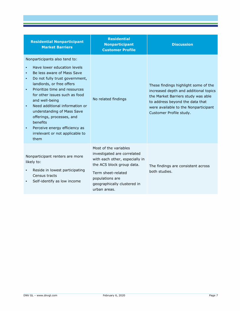
Nonparticipants also tend to:
• Have lower education levels
• Be less aware of Mass Save
• Do not fully trust government,
landlords, or free offers
• Prioritize time and resources
for other issues such as food
and well-being
• Need additional information or
understanding of Mass Save
offerings, processes, and
benefits
• Perceive energy efficiency as
irrelevant or not applicable to
them
No related findings
These findings highlight some of the
increased depth and additional topics
the Market Barriers study was able
to address beyond the data that
were available to the Nonparticipant
Customer Profile study.
Nonparticipant renters are more
likely to:
• Reside in lowest participating
Census tracts
• Self-identify as low income
Most of the variables
investigated are correlated
with each other, especially in
the ACS block group data.
Term sheet-related
populations are
geographically clustered in
urban areas.
The findings are consistent across
both studies.

DNV GL – www.dnvgl.com February 6, 2020 Page 8
Residential Nonparticipant
Market Barriers
Residential
Nonparticipant
Customer Profile
Discussion
Moderate income nonparticipants
are more likely to reside in higher
participating Census tracts.
Most of the variables
investigated are correlated
with each other, especially in
the ACS block group data.
Term sheet-related
populations are
geographically clustered in
urban areas.
On the surface, these findings seem
contradictory. However, it is
important to note that the two
studies used different definitions of
moderate income. In the Market
Barriers study, the definition of
moderate income was $50,000 to
$75,000. In the Customer Profile
study, the definition of moderate
income was $40,000 to $59,999.
This means that part of the
moderate income group in the
Market Barriers study falls into the
“average or higher income” category
for the Customer Profile study. When
this cross-categorization is taken
into account, the findings are largely
consistent across both studies.
1.3 Methodology overview
DNV GL conducted the following tasks:
1. Prepare data. These analyses utilized three different data sets: block group data, individual-level data,
and enhanced individual-level data.
a. DNV GL developed the block group-level data as part of the overall project’s first deliverable (Low
Participation Table). We enhanced these data with ACS variables covering additional income
categories, construction date, heating fuel type, and urban/rural status.
b. We prepared the individual-level data as part of the Nonparticipant Profile Study’s second Deliverable
(Participant-Nonparticipant List; “PNP list”). This deliverable was primarily intended to serve as a
sample frame for surveys conducted as part of a parallel project. We enhanced this data with a
calculated renter flag.
c. We added the enhanced individual-level Experian data to the individual-level data set. However,
because these data are available for Eversource customers only, this data set has more variables but
fewer customers than the individual-level data.
2. Conduct block group-level analyses. These analyses included correlations and ordinary least squares
(OLS) regression models. Dependent variables for these models were location participation rate and the
ratio of savings to consumption (savings/consumption); independent variables were proportions of

DNV GL – www.dnvgl.com February 6, 2020 Page 9
households in block groups with certain characteristics such as moderate income. The independent
variables were based on ACS data.
3. Conduct individual-level analyses. We conducted analyses parallel to the block group-level analyses
using the individual-level data. The dependent variables for these models were account participation and
savings/consumption. Independent variables were individual-level variables reflecting demographic
characteristics available statewide through sources such as the Tax Assessor data (multifamily, year of
construction) and those available only for Eversource through Experian data (income, language).
Throughout the analysis phase, DNV GL referenced the 2013-2017 Residential Customer Profile Study report
which contains similar analyses. When discrepancies were found, we conducted extra analysis to resolve the
differences.
1.3.1 Provisions
The following provisions and limitations pertain to this study.
1. The core data used for this study only covers the five-year period from 2013 – 2017, and
participation in PA programs. The populations under consideration might have participated prior to
and/or after this window or may have participated in programs sponsored by organizations other than
the PAs.
2. This study excludes savings from several sources: upstream programs, behavioral programs, and
delivered fuel projects (the latter for some analyses). The upstream and behavioral programs account
for approximately 8% of the total residential electric and 14% of the total residential gas savings from
2013-2017. Delivered fuel savings were excluded because we do not have reliable information for the
total consumption of delivered fuels. Therefore, the ratios in this report that rely on savings (e.g.,
savings/consumption) are impossible to calculate for delivered fuels. Participation in delivered fuel
projects is included in our (binary) participation metrics.
3. There is no perfect way to measure or define “participation.” This study utilized four different
definitions, each of which has strengths and weaknesses.
a. Location participation measures whether a building participated. Location participation is similar to
coverage rate. It is best used to answer questions such as, “How many buildings did the program
touch, regardless of size?” A strength of location participation is that it is stable over time, so it is
useful for time-series analyses. Weaknesses of location participation are: It overstates participation
of multifamily (MF) buildings because a location is considered a participant if any sub-unit within the
building has participated; single-family (SF) homes count the same amount as MF buildings; and
building-level data grain does not match the ACS data grain, which is at the household level.
b. Consumption-weighted location participation uses location participation multiplied by the total
consumption associated with each location. This metric gives a sense of how much of the underlying
consumption the programs addressed. It is best used to account for the impact differences between
SF and MF locations and to answer questions such as, “How well has the program addressed large
customers?” The strengths of this variable are that it is stable over time, like location participation,
and that it differentiates between SF and MF buildings. Weaknesses are that it overstates
participation at MF locations to an even greater extent than location participation due to the effects
of very large MF buildings; it is not at the same grain as ACS variables; and it can be difficult to
interpret.

DNV GL – www.dnvgl.com February 6, 2020 Page 10
c. Account participation measures whether a unique account ID has participated at least once over a
certain timeframe. This variable is best used when one wants to answer questions about individuals
who participated, such as, “What income levels did past participants have?” Strengths of this metric
are that it is closest to the same grain as the ACS variables; it is directly accessible from PA tracking
data; and it is relatively easy to interpret. The main weakness of this variable is that it is not stable
over time. Account IDs change when new residents move in or out of a specific dwelling, so a high
proportion of dwellings with frequent resident turnover (e.g., rented apartments) will tend to lower
account participation rates by increasing the denominator while not changing the numerator.
Account participation also does not accurately capture participation at the individual housing unit
level in master-metered MF buildings.
d. Savings/consumption measures the ratio of savings achieved in a block group or for a specific
account between 2013-2017 and the average consumption for the block group or account from
2013-2017. The strengths of this metric are that it shows depth of participation and locations with
greater consumption (i.e., large MF buildings) have greater relative weight in the analyses. This also
creates a limitation: those large consumers can dominate block-group sums and averages while they
do not have any exceptional weighting in individual account-level analyses. Other limitations of this
metric are that it does not fully account for consumption added for new construction, and at the
account level, it does not fully capture savings that occurred at the same location under a different
account-holder.
4. Several limitations apply to the account-level analyses:
a. The individual and enhanced individual-level analyses are limited to unique 2017 accounts.
The analyses cover participation for these accounts at any time between 2013-2017. However, the
analyses do not cover 2013-2017 participation for accounts that were not active in 2017.
b. Any participation that occurred by accounts that did not exist in 2017 is not represented.
This particularly affects renters, who are a key population of this study. For example, if
someone living at a home participated in 2015, then moved out in 2016, and a new person moved in
in 2017, the 2015 participation would not be modeled.
c. Accurately accounting for participation in master metered multifamily buildings, especially
low-income multifamily buildings, has proven difficult with the data available from some
PAs. Some PAs track participation of individual units within multifamily buildings, but other PAs track
participation only at the whole building level. The evaluation team cannot account for data that does
not exist. We have used location and consumption-weighted location participation to partially account
for the whole-building approach of some PAs, but these participation variables have their own
limitations. Individual household characteristics also cannot be modeled at the building level.
d. The enhanced individual-level analyses are limited to Eversource accounts. The Experian
data with which we enhanced the data were only available for Eversource customers. We attempted
to integrate audit data from the other PAs that contains some similar data. However, the audit data
did not cover other PAs’ customer base sufficiently to aid the analyses in this study.
e. The method used to identify renters in the statewide data set is not completely accurate.
While this method does highly correlate with more rigorous ACS and Experian methods of
determining renter status, it is not a perfect correlation. The method will undercount long-tenured
renters and overcount changes to account status for other reasons (e.g., name change due to
marriage/divorce).

DNV GL – www.dnvgl.com February 6, 2020 Page 11
f. The ACS definition of multifamily (5+ units) does not fully align with Tax Assessor data.
The Tax Assessor data has categories for 4-8 units and over 8 units.
5. The block group and individual analyses utilize different data grains. The block group-level
analyses use location and consumption-weighted location participation. The individual-level analyses use
account participation. The difference in data grain means that caution should be exercised when directly
comparing the results across the levels of analysis. However, the fact that the results of all three
analyses are similar is positive. This indicates a level of consistency in the real-life situation that the
models are trying to capture. Furthermore, the previous memo that reported on block group-level
results included account participation, and the outcomes for account and location participation were
highly congruent in those findings.
6. The analyses presented in this study are not adversely affected by small populations meeting
the term sheet characteristics. The way to interpret the block group level correlations is “as the
proportion of households that meet term sheet characteristics increases, the rate of participation tends
to decrease.” That the term sheet households are relatively rare does not drive the relationship; as you
get a higher concentration of those households in a block group, we expect the (total) participation rates
in that block group to decrease. For the individual-level models, we are modeling the probability that a
particular house will participate based on the term sheet (and other) characteristics. The individual
model looks at the participation rate of the accounts with that characteristic, rather than the rate of the
characteristic in the participant population.
7. The study did not examine differential funding levels. PA funding for low income programs is not
necessarily uniform throughout the state. This study did not factor any such differences into the
analyses.

DNV GL – www.dnvgl.com February 6, 2020 Page 12
2 INTRODUCTION
2.1 Study purpose, objectives, and research questions
DNV GL carried out the Residential Nonparticipant Analysis Study (MA19X06-B-RESNONPART; “NPA”) for the
Massachusetts Program Administrators (PAs) and Energy Efficiency Advisory Council (EEAC) Consultants
from February 1, 2019, to September 30, 2019. The study’s overall purpose was to assess relationships
between participation rates and the variables specified in the PAs’ October 19, 2018 term sheet, which
stipulates:
“Special Focus on Renters, Moderate Income, Non-English Speaking, and Small Business Customers:
The Program Administrators will conduct tailored evaluations in 2019 that address participation
levels and potential unaddressed barriers for (a) businesses (small, medium and large) and (b)
residential customers by income levels and by non-English speaking populations (utilizing proxy
methods that do not rely on specific income or demographic information from Mass Save®
participants). The Program Administrators will leverage the existing EM&V framework, and present
full results of the studies to the EEAC.” 3
This study was developed to provide information relevant to the term sheet stipulation. The study
objectives, as established by the working group, are as follows:
1. Quantify recent levels of participation in PA programs for moderate-income customers, renters, and non-
English-speaking customers
2. Quantify how various factors (including but not limited to income level, language barriers, building
ownership, and single or multifamily) are associated with participation in Mass Save residential
programs
3. Address the possibility of ecological fallacy4 when using block group-level variables
4. Establish a baseline level of participation that can be used to assess the effectiveness of PA efforts to
increase outreach
This report addresses the first 3 objectives. It presents the results of the tasks involving statistical modeling
to characterize the relationships between the term sheet variables, participation, and other available
demographic variables. The multiple levels of modeling also helped determine the extent of ecological fallacy
in the block group-level analyses. We also provide implications and recommendations derived from those
findings. There are two additional, separate deliverables that add to the information presented in this report:
• A “low participation” table that shows levels of the term sheet variables and location participation rates
by town and block group level. This deliverable addresses objectives 1 and 4. A copy of the town-level
data provided by this deliverable is included in Appendix B (Section 7) of this document.
• A series of bivariate maps that provide visualizations of areas with high concentrations of the term sheet
characteristics and low participation rates. A copy of this deliverable is included in Appendix C of this
document.
This study provided a foundational analysis of participation patterns to identify underserved customers. This
analysis fed into a subsequent study called the “Residential Nonparticipant Market Characterization and
Barriers Study” (Market Barriers Study). The Market Barriers Study was a market assessment that
3 http://ma-eeac.org/wordpress/wp-content/uploads/Term-Sheet-10-19-18-Final.pdf
4 Ecological fallacy occurs when one makes conclusions about an individual based on group-level variables.

DNV GL – www.dnvgl.com February 6, 2020 Page 13
conducted primary research (including surveys and in-depth interviews) to explore market barriers for the
underserved customer segments, and to develop recommendations to more effectively reach those
segments.

DNV GL – www.dnvgl.com February 6, 2020 Page 14
2.2 Organization of report
The remainder of this report focuses on the first two objectives listed above, and is structured as follows:
• Section 3 – Methodology and approach
• Section 4 – Analysis and results
• Section 4.1 – ACS variable correlations
• Section 4.2 – Electric location participation findings
• Section 4.3 – Electric savings/consumption findings
• Section 4.4 – Gas location participation findings
• Section 4.5 – Gas savings/consumption findings
• Section 4.5.4 – Conclusions, recommendations, and considerations
• Section 6 – Appendix A – Participant/nonparticipant list preparation
• Section 7 – Appendix B – Low participation table
• Section 8 – Appendix C – Bivariate maps
• Section 9 – Appendix D - Close-up hotspot maps

DNV GL – www.dnvgl.com February 6, 2020 Page 15
3 METHODOLOGY AND APPROACH
This section provides more detail on the study tasks. In general, this study uses the definition of participant
from the MA Technical Reference Manual (TRM): a participant is “a customer who installs a measure through
regular program channels and receives any benefit (i.e., incentive) that is available through the program
because of their participation.”
3.1 Participation by block group list preparation
The study’s first objective was to quantify recent levels of participation of the populations defined by the
term sheet variables. This objective was achieved through a separate deliverable called the Low Participation
Table, also referred to as Deliverable 1. This is an Excel workbook that presents, by census block group, the
proportion of households that meet each term sheet variable criteria and the consumption-weighted location
participation of that block group. DNV GL also aggregates the block group data at the town5 level. Controls
allow the PAs to filter the table by electric PA and gas PA, and sort by town name and participation rate. The
workbook has separate worksheets for electric-only, gas-only, and dual-fuel participation. A copy of this
Excel book is embedded in Appendix B of this report.
The data used for the Low Participation Table includes PA billing and tracking records for 2013-2017,
processed by DNV GL’s MA data management team. After combining the individual years of data, we made
four changes to the data to prepare it for the Low Participation Table:
1. Using building type information from tax data and a string search on customer names (e.g. names that
included various permutations of “HOUSING AUTHORITY”), we identified housing authorities and
subsidized multifamily housing in the C&I billing data. These records were added to the residential billing
data to account for the fact that buildings with C&I accounts housing low-income tenants participate
through the PAs’ low-income initiatives. Without including the consumption of these buildings, the
denominator for any savings achieved calculations would be incorrect for low-income participants.
2. For accounts that had bad address information for one or more years but currently have good address
information, we back-filled that information to make sure that each account is assigned to the correct
block group for as many years as possible.
3. We removed a single outlier/error in the National Grid data that had 1-month consumption of greater
than 1 million kWh.
4. With guidance from the PAs, we removed non-gas MMBTU savings (i.e., MMBTU savings in the electric
tracking data for delivered fuel projects) from the tracking data due to inconsistencies. We did not,
however, remove delivered fuel participants from our participant counts.
3.2 Participant-Nonparticipant list preparation
The primary purpose of the Participant-Nonparticipant (PNP) list was to provide a population for a related
study to draw samples of current residents to survey. Key characteristics needed by the survey study were
addresses, block groups, and 2013-2017 participation status (as a binary variable). Because some
residentials buildings, particularly housing authorities, can be on C&I rates, DNV GL needed to merge C&I
and residential billing data to provide the survey team with a complete population. DNV GL was also able to
leverage this data for individual-level analyses as a secondary use. DNV GL prepared the Participant-Non-
5 Towns as defined by the Tax Assessor.

DNV GL – www.dnvgl.com February 6, 2020 Page 16
participant (PNP) list using the following process. This was a completely separate effort from the block group
list preparation.
1. Combined 2013 – 2017 residential tracking data6
2. Merged 2017 Residential and C&I billing data
a. Added geocode information
b. Added tax assessor information
c. Filtered out C&I accounts (e.g., streetlights and nonresidential locations)
3. Identified participants from the tracking data
4. Identified most recent account holder based on mid-2018 lists provided by PAs
The result of this process was a data file at the account data grain of unique residential and multifamily
accounts billed in 2017, with account and location participation variables based on the 2013-2017
(residential only) tracking data and with additional location-level data such as Tax Assessor information
appended. The final number of unique account IDs by fuel and PA are shown in Table 3-1. Detailed data
preparation methods are described in Appendix A.
Table 3-1. Final record counts by fuel and PA
Fuel
PA From Residential Billing
From C&I Billing1 Total
E Cape Light Compact 190,212 1,703 191,915
E Eversource 1,245,185 34,552 1,279,737
E National Grid 1,168,581 38,961 1,207,542
E Unitil 29,103 354 29,457
Total Electric 2,633,081 75,570 2,708,651
G Berkshire 35,223 621 35,844
G Columbia 348,951 3,262 352,213
G Eversource 315,619 3,375 318,994
G Liberty 51,867 147 52,014
G National Grid 845,449 8,989 854,438
G Unitil 16,641 134 16,775
Total Gas 1,613,750 16,528 1,630,278
Grand Total 4,246,831 92,098 4,338,929
1 C&I records were included to ensure we accounted for multifamily buildings; excluding accounts positively identified as non-residential such as
businesses, streetlights, and cellphone towers.
Besides the difference in data grain (block group versus account), there are three key differences between
the block group list and the PNP list. First, the block group list did not attempt to match specific participating
accounts with specific billed accounts; it summed all participation and all consumption. In contrast, the PNP
list does match specific account ids across billing and tracking databases. Second, the PNP list contains only
information from accounts billed in 2017. In contrast, the block group list contains information for accounts
6 While we included C&I billing data to ensure we had all potential residential buildings, we includined only residential tracking data.

DNV GL – www.dnvgl.com February 6, 2020 Page 17
billed anytime between 2013 and 2017. Finally, the PNP list contains more C&I records (billed in 2017) than
the block group list. The block group list added only C&I records that could be positively identified as
housing authorities or low-income housing. In contrast, the PNP list included all C&I records and only
excluded those that could be positively identified as not residential. Thus, the PNP list errs on the side of
including C&I account that actually are not residential. This was partly because the primary purpose of the
list was for survey sampling purposes and the surveys would have the ability to screen out truly non-
residential locations.
3.2.1 Renter flag
This section outlines the steps we used to prepare the data before identifying likely renters. The goal of this
data processing was to identify all accounts in the PNP list that are likely renters. The PAs did not have
direct information on renter status. Therefore, DNV GL had to implement a logical process to determine if an
account was a likely renter. This determination had to be based on data available for all PAs, which was
limited. We identified high turnover rate (i.e., a higher number of accounts associated with a location from
2014-2017) as a proxy for renter status.
This method has limitations and relies on several assumptions. We assumed that residents in rented
properties will move in and out more quickly than in non-rented properties. We set a threshold on the
number of account changes to represent this tendency. However, an account change does not necessarily
mean a renter turnover or even a sale or change of ownership, and the threshold approach underrepresents
long-tenured renters. Without additional information to draw on, we also assumed condos are owned rather
than rented, so rented condos are also underrepresented. Unfortunately, there is no good way to resolve
these limitations without conducting surveys.
However, our approach provides a means of assigning likely renter status using data readily available from
all PAs. Experian uses a much more robust approach to assigning likely renter status.7 This approach begins
with self-reported data from surveys, then includes a comparison between the names in the Tax Assessor
records and the current resident, and finally includes statistical interpolation to fill in otherwise missing data.
Despite the limitations of our approach, we agree with Experian’s assignments 90% of the time.8
Renter flag definition
The data processing began with the Participant-Nonparticipant (PNP) list produced as part of Deliverable 2.
This list was based on all accounts billed in 2017. Using the locations (latitude and longitude pairs) in the
PNP list, we identified all accounts associated with those locations from the combination of the 2015-2017
C&I billing data and the 2014-2017 residential billing data.
We then counted the number of 2014-2017 accounts associated with each location between 2014 and 2017
by PA and fuel type. We counted accounts by PA and fuel type at a location, as some locations will be served
by both a gas and an electric PA but others will not, resulting in variations in the number of expected
accounts at a given location.
Finally, lacking any other information, we assumed condos are owned and flagged condo locations by
looking for permutations of “CONDO” in the customer name and using the tax assessor building types that
correspond to condos. If any account at a given location was flagged as a condo, we classified the location
(latitude and longitude) as a condo.
7 Based on the data dictionary provided with Experian’s data.
8 For Eversource, which is the only PA for which we have Experian data.

DNV GL – www.dnvgl.com February 6, 2020 Page 18
Table 3-2 and Table 3-3 present the number of accounts per location for electric and gas accounts
respectively. For electric, most locations had two or fewer accounts within the four-year timespan of 2014-
2017. For gas, most locations had three or fewer accounts within the four years.
Table 3-2. Number of electric accounts per location, 2014-2017
Number of Accounts Percentage of Locations Cumulative Percentage
1 27% 27%
2 39% 66%
3 15% 82%
4 5% 87%
5 2% 89%
6 3% 92%
7 2% 93%
8 1% 94%
9 1% 95%
10+ 5% 100%
Table 3-3. Number of gas accounts per location, 2014-2017
Number of Accounts Percentage of Locations Cumulative Percentage
1 25% 25%
2 14% 39%
3 28% 67%
4 16% 83%
5 3% 85%
6 3% 89%
7 2% 91%
8 3% 93%
9 1% 95%
10+ 5% 100%
Next, we compared Experian data available for Evesrource, which has a flag for likely renters, to our data on
the number of accounts per location to determine the number of accounts at a location over a four year
period that indicates a likely renter. Table 3-4 presents the number of accounts per location for (Eversource)
records that Experian flagged as likely homeowners and likely renters, respectively. Ninety percent of
locations that Experian indicated were likely owned had 3 or fewer accounts between 2014 and 2017, while
56% of locations Experian indicated were likely rented had 4 or more accounts between 2014 and 2017. We
selected 4 or more accounts as our rental threshold. At this threshold, the majority of locations are rented
according to Experian and almost all of the locations with 3 or fewer accounts are reported as owned by
Experian.9
9 It is difficult to identify single-family homes that are renter-occupied.

DNV GL – www.dnvgl.com February 6, 2020 Page 19
Table 3-4. Number of accounts per location for Experian’s likely renters not flagged as a condo
location
Number of accounts
Percentage of Locations
Cumulative Percentage
1 14% 14%
2 20% 34%
3 10% 44%
4 10% 54%
5 7% 61%
6 7% 68%
7 5% 73%
8 5% 78%
9 3% 81%
10+ 19% 100%
Figure 3-1 presents how the initial renter flag was assigned. We processed electric and gas accounts
separately, and set the location to “rented” if either analysis indicated it. Finally, we checked our assignment
against the Experian “likely renter” assignment. Both assignments agreed 90% of the time (see Table 3-5).
Figure 3-1. Renter flag definition
Table 3-5. Experian renter flag location comparison
Category Percentage
Match 90%
Don't Match 10%
Other methods investigated
We investigated the feasibility of using two other methods to determine renters, both of which relied on
text-based matches on account owner names. The first alternative method compared the PA’s account
owner name to the tax assessor’s plot owner name. The second method attempted to track changes in the
account owner name(s) associated with a location across the years of available billing data. We determined
that both methods were impractical because of the limitations of matching text strings for the volume of
data involved in this project. The method we described using account ID is simpler, more reliable, and has a
90% agreement with Experian’s assignments. We determined that achieving an agreement rate better than
90% using the name matches is unlikely and even if possible, would have used a large portion of the
remaining project budget.
DNV GL – www.dnvgl.com February 6, 2020 Page 20
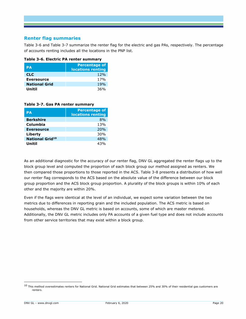
Renter flag summaries
Table 3-6 and Table 3-7 summarize the renter flag for the electric and gas PAs, respectively. The percentage
of accounts renting includes all the locations in the PNP list.
Table 3-6. Electric PA renter summary
PA Percentage of
locations renting
CLC 12%
Eversource 17%
National Grid 19%
Unitil 36%
Table 3-7. Gas PA renter summary
PA Percentage of
locations renting
Berkshire 8%
Columbia 13%
Eversource 20%
Liberty 30%
National Grid10 48%
Unitil 43%
As an additional diagnostic for the accuracy of our renter flag, DNV GL aggregated the renter flags up to the
block group level and computed the proportion of each block group our method assigned as renters. We
then compared those proportions to those reported in the ACS. Table 3-8 presents a distribution of how well
our renter flag corresponds to the ACS based on the absolute value of the difference between our block
group proportion and the ACS block group proportion. A plurality of the block groups is within 10% of each
other and the majority are within 20%.
Even if the flags were identical at the level of an individual, we expect some variation between the two
metrics due to differences in reporting grain and the included population. The ACS metric is based on
households, whereas the DNV GL metric is based on accounts, some of which are master metered.
Additionally, the DNV GL metric includes only PA accounts of a given fuel type and does not include accounts
from other service territories that may exist within a block group.
10 This method overestimates renters for National Grid. National Grid estimates that between 25% and 30% of their residential gas customers are
renters.

DNV GL – www.dnvgl.com February 6, 2020 Page 21
Table 3-8. PNP renter flag block group comparison with ACS block group percent renter
Difference in % renter1
% of Electric PA Block Groups
% of Gas PA Block Groups
0% - 10% 43% 33%
11% - 20% 29% 28%
21% - 30% 15% 18%
31% - 40% 7% 9%
41% - 50% 3% 4%
51% - 60% 1% 2%
61% - 70% 1% 2%
71% or more 0% 3%
1 Calculated as the absolute value of the difference between the ACS percent renter and the PNP percent renter by block group.
3.2.2 Modeling
DNV GL analyzed three levels of models: block group, individual, and enhanced individual. We modeled
electric and gas participation separately, using the same methods in both cases.
1. Block group-level models. For these models, the dependent variable is location participation,
consumption-weighted location participation, or savings/consumption within a block group. Predictor
variables are block group-level American Community Survey (ACS) variables expressed as proportions
of locations or households that match the term sheet variables. These models utilize the most readily
available data and do not contain personal identifying information. However, because they operate on
proportions of block groups, they can be difficult to interpret and are susceptible to ecological fallacy.
2. Individual-level models. These models use the binary definition of participation at the account level and
savings/consumption computed at the account level. They predict participation using individual-level
variables available from the unified Massachusetts residential database prepared for the Residential
Customer Profile Study (RCPS). This database includes information from the PAs’ billing and tracking
data as well as information appended from the Massachusetts Tax Assessors data.
3. Enhanced individual-level models (available for Eversource only). These models are similar to the
standard individual-level models, but they include additional location-level variables available through
third-party data sources, specifically Eversource’s Experian data. DNV GL attempted to integrate audit
data available for the other PAs. Due to a high percentage of missing values in the variables of interest,
pertinent data was available for less than 100 accounts. Therefore, we left the audit data out of this
analysis to help reduce evaluation costs and used only the Experian data for Eversource.
Block group-level models
The initial models predict block group-level participation rates using variables based on block group-level
ACS data and US Census Urban and Rural Classification data. Participation rates are informed by program
participation data from 2013 to 2017 and 2013-2017 billing data. For the electric analyses, we included only
block groups where one of the electric PAs was listed as a utility of service by the Department of Public
Utilities (DPU). For the gas analyses, we included block groups where one of the gas PAs was listed as the
utility of service by the DPU.
We used three different definitions of participation, each calculated at the block group level. The
participation variables are defined as:

DNV GL – www.dnvgl.com February 6, 2020 Page 22
• Location-level participation: Location-level participation is calculated as the number of unique
locations that participated at least once between 2013 and 2017, divided by the number of unique
locations in the 2013-2017 billing data.
• Consumption-weighted participation: is defined as the sum of 2017 consumption for any locations
that participated at least once between 2013-2017 divided by the sum of 2017 consumption for all
locations.
• Savings/Consumption: is defined as the sum of 2013-2017 savings divided by the average 2013-
2017 consumption, both taken at the block group level. We drop block groups for whom the metric
exceeds 1.11 While a value greater than 1 is theoretically possible, it is extremely rare, and these
instances most likely represent substantial new construction occurring in the block group.
����� ��� ����� ������
���������=
��2013 − 2017 ��������� !"
#�������2013 − 2017 ������������ !"
The predictor variables include ACS variables associated with the term sheet:
• Moderate income: We used the proportion of households with incomes between 56 and 85% of
statewide median income12 (based on ACS variables B19001e9, B19001e10, B19001e11, and S1903e2).
Note, this is a proxy for true moderate income in two different ways; moderate income is defined as
61% to 80% of state median income, factoring in household size. We had only block-group level data.
Thus, we chose income ranges available in the ACS data that most closely approximated the eligibility
ranges set by Mass Save for a household size of 2.
• Renter-occupied housing: The proportion of occupied households in the block group that are renters
(based on ACS variables B25003e, B25003e3)
• Multifamily housing: The proportion of occupied households in the block group living in buildings with
5 or more units (based on ACS variables in table B25024)
• Limited English-speaking households: The proportion of households in the block group reporting as
speaking limited English at home (based on ACS variables in table C16002)
DNV GL also investigated the relationships between participation and several other ACS variables, including:
• Low income: Defined as the proportion of households with less than 56% statewide median income13
(based on ACS variables B19001e1, B19001e2, B19001e3, B19001e4, B19001e5, B19001e6, B19001e7,
and B19001e8). This variable is a proxy for low income, which is officially defined as less than or equal
to 60% of state median income.
• Average or higher income: Defined as the proportion of households with greater than moderate
income (based on ACS variables B19001e1, B19001e12, B19001e13, B19001e14, B19001e15,
B19001e16, B19001e17). Note that this definition may not be considered truly high income by other
standards. We include the variable as a comparison point for moderate income.
• Construction year: Defined as the proportion of housing units built within the following ranges of
years: before 1949, 1950-1969, 1970-1989, 1990-2009, and 2010 or later (based on ACS variables in
table B25034)
• Heating fuel type: Defined as the proportion of occupied housing units with primary heating fuels of
natural gas, electric, or non-utility fuels. Non-utility fuels include all fuel types other than natural gas or
11 0.3% of block groups in the electric analysis were affected. 0.1% of block groups were affected in the gas analysis.
12 Based on the grand median statewide income, independent of household size.
13 Based on the grand median statewide income, independent of household size.

DNV GL – www.dnvgl.com February 6, 2020 Page 23
electric, such as fuel oil, propane, kerosene, wood, and solar (based on ACS variables from table
B25040).
• Urban/rural: Defined using the 2010 U.S. Census definition of urban and rural at the block level. The
block level is smaller than the block-group level. All homes in urban blocks were coded as urban, and
then we computed the proportion of urban homes within a block group based on the number of homes
in the urban blocks divided by the total number of homes in the block group. Rural was calculated in the
same way. It should be noted that the majority of blocks in MA are coded as urban (there are
approximately 4 times as many urban as rural blocks). Furthermore, according to the 2010 Census,14
92% of the state population lives in urban areas, which account for 38% of the land area.
The first step in our analysis was to look at zero-order correlations between each of the participation
variables and each of the ACS variables. These results are discussed in detail in Section 4.1. These
correlations estimate the direct relationship between participation and the ACS variables of interest. They
represent the simplest and most direct relationship between the variables of interest. Because they
represent the relationships between only two variables at a time, they do not account for nuances or the
effects of multiple variables.
For example, both renting and limited English are positively correlated with each other and negatively
correlated with participation rates. The correlations themselves do not provide any insight into how the
three variables relate. One possibility is that the three correlations are completely independent. Another
possibility is that the relationship of one variable is explained by another. For example, if limited English
speakers are more likely to rent, and renters are less likely to participate, does renter status explain why
limited English speakers are less likely to participate? A third possibility is that there is another variable at
work. In this case, perhaps renters and limited English speakers both tend to have lower incomes, and it is
lower income that explains decreased participation. Regression models allow one to account for these
interrelated effects.
The next analytic step was to use regression modeling to estimate the independent and interrelated effects
of the ACS variables on participation. We used ordinary least squares (OLS) to estimate the following
general block group participation model. We repeated this model for location participation and consumption-
weighted location participation. The primary model15 estimated participation rate as a function of the
proportion of moderate-income homes, the proportion of renter-occupied housing units, the proportion of
multifamily housing units, and the proportion of limited English speaking households. We also ran additional
models using different permutations of the ACS variables to better understand how the term sheet variables
interacted with each other and the non-term sheet variables. These results are discussed in Section 4.2.
For variables that are perfectly collinear, meaning that there is a mutually exclusive relationship between
them (e.g. urban and rural), one of the variables must be dropped from models as there is no variation for
the model to pick up. As an example, the proportion of rural PA households is 1 minus the proportion of
14 https://www2.census.gov/geo/docs/reference/ua/PctUrbanRural_State.xls
15 $� = % + Β()�*� + Β+,���� + Β-).� + Β/0��� + 1
Where:
- $� is the participation rate
- )�*� is the proportion of households at 56 - 85% of statewide median income
- ,���� is the proportion of renter occupied housing units
- ).� is the proportion of housing units in 5+ unit buildings
- 0��� is the proportion of limited English-speaking households

DNV GL – www.dnvgl.com February 6, 2020 Page 24
urban PA households. Because these two variables contain the same information and are linearly related to
one another, they cannot both be included in the same model. The variable dropped from the model can be
interpreted as the reference case, meaning that the coefficient for urban in this example is the impact of
urban vs. rural. For most models, we dropped the proportion of households above 85% of the statewide
median income, the proportion of households built in 1950 or later, the proportion of households with non-
utility heating, and the proportion of rural households.
Individual-level modeling
The primary purpose of the individual modeling was to assess whether the findings based on the block
group-level models were consistent when using individual-level models. Because the block group-level
models are based on proportions of households within a geographic area, they are susceptible to the
ecological fallacy. That is, an association between two variables in the block group-level models does not
necessarily link the two variables at an individual household level. For example, moderate-income and low
participation were negatively correlated in the block group models. This means that as the proportion of
moderate-income households increases, the participation rate of the block group decreases. However, it
should not be interpreted as “moderate-income households are less likely to participate.” Such an
interpretation requires individual-level modeling.
The drawback of the individual-level modeling is that it is more difficult to reliably determine demographic
characteristics at this level. The ACS variables are readily accessible, but the PAs do not track most of those
demographic variables at the account level in either their billing or program tracking databases. Obtaining
variables at this data grain often requires costly data purchases. In some cases, the individual data provided
are derived from the same aggregate data that we are trying to test, and therefore are subject to the same
ecological fallacy concerns. We ran models that paralleled the block group models as closely as possible
using the account-level information available from the PA billing and tracking databases. Experian
demographics data was available for Eversource customers, but not other PAs.
• Account participation: For the individual-level models, we used account participation as the
dependent variable. Account participation is closest in data grain to the individual-level variables we
used as independent variables in these models. The two primary drawbacks of using account
participation are that it can fail to represent participation in master-metered multifamily buildings and in
cases where the tracking system does not have unit-level measure records, and it underrepresents
participation in time-series analyses.
The first limitation of failing to represent all master-metered multifamily participation is impossible to
completely overcome. The best option is to use location participation. However, using location
participation as a dependent variable would put the dependent and independent variables at different
data grains. This introduces complications such as how to calculate individual-level variables such as
income or primary language at a location level. Location-level participation is also susceptible to a bias
for master-metered multifamily participation in the opposite direction as account-level participation.
Because location-level participation was set to 1 if any of the units at a location participated, it tends to
overrepresent participation because larger buildings (those with more units) have more chances for at
least one unit to participate. Thus, location-level participation assessed at the account level results in

DNV GL – www.dnvgl.com February 6, 2020 Page 25
every account within a participating location being set as a participant, which definitely over-represents
participation.16
The time-series limitations for account-level participation were mostly absent in the individual-level
modeling because of the way we prepared the data sets. The basis of the data were active accounts in
2017. Because we limited the basis to a single year and associated any participation that occurred from
2013-2017 to that single year of billed accounts, the data set was able to essentially avoid any time
series variability.
• Savings/consumption: For the individual-level metric, we start with the accounts in the PNP list. This
list is based on accounts active in 2017 because its initial purpose was to provide a sample for the
qualitative surveys. Using this starting point allows the study to add in a savings/consumption metric at
the individual level and still meet the established reporting timeline.
Calculating the individual-level metric presents some challenges. First, not all accounts active in 2017
were also active all the way back to 2013, and the number of active accounts gets smaller the further
we go back in time. Furthermore, some accounts’ consumption in the first active year is extremely low
(<1,000 kWh). To derive a typical consumption level for the account against which to normalize the
savings, we remove the years with <1,000 kWh of consumption before averaging the annual
consumption values we have for each account. For the numerator, we include any savings we have
records of. Similar to the block-group-level metric, we drop any account whose metric exceeds 1.17 We
calculate the formulation as follows:
2�*���*�� ����� ������
���������=
��2013 − 2017 ������+3(45 �678"
#������ ���������+3(-9+3(4
The strength of this metric is that it presents a more scalable metric of participation than account- or
location-level participation rates.18 Whereas single-family and large multifamily sites count equally in
location participation, the savings/consumption metric scales with the energy-saving opportunities
inherent in larger sites like high-rise multifamily buildings.
This metric also has several limitations. As noted above, the individual-level formulation fails to account
for the participation of previous residents (accounts) that the current resident may be benefiting from.
This limitation is more relevant to more transient populations such as renters, which are one of this
study’s key populations of interest. We also cannot identify situations where savings were recorded in
the tracking database associated with a single site but were in reality distributed across multiple sites.
DNV GL has seen an example of this in another study when all the fire stations in a city participated in a
program. There were savings across approximately 10 stations, but all of the savings were tracked at a
single station. When these situations occur, it can cause savings to exceed consumption. Because we
excluded cases where the metric exceeded 1, any cases such as these are not in the present analysis.
We prepared the independent variables slightly differently for the standard (all PA) models and the
enhanced (Eversource-only) models. For the enhanced models, we assigned the variables based only on
Experian data whenever possible.
16 The situation where a building owner retrofits lighting in common areas is an example of when this could happen. In this case, one could argue
that all tenants in the building benefit from that participation. However, that level of indirect benefit was not the focus and is not captured in
this study. 17 This affected 4% of electric accounts and 9% of gas accounts.
18 This should not be taken or construed as a better or more accurate representation of participation than metrics used in other studies, and is not a
subjective statement on the quality, accuracy, or appropriateness of those other metrics to address different research questions.

DNV GL – www.dnvgl.com February 6, 2020 Page 26
• Moderate income:
- (statewide models) We attempted to use building value and value per square foot data available
from the Tax Assessor’s data as a proxy for income in the all PA data set. However, all such
variables we were able to create using the Tax Assessor data failed to correlate with income in the
Experian data set, so we decided it was not a viable proxy. Thus, we did not have a viable income
variable in the all-PA dataset.
- (enhanced models only) The Experian data includes a variable that listed income ranges. The ranges
are in $15,000 or greater increments. As we did for the ACS data, we selected the two ranges that
most closely corresponded to the definition of moderate income. Based on grand statewide median
income, the moderate-income range in Massachusetts is approximately $41,000 to $63,000. The
two ranges available from Experian data that we coded as moderate-income were $35,000 to
$49,999 and $50,000 to $74,999.
• Renter:
- (statewide models) We coded renter as a dummy variable in the all PA dataset based on the
description in section 0.
- (enhanced models) We coded a dummy variable as 1 if Experian listed the record as a renter or
likely renter.
• Multifamily housing:
- (statewide models) We coded multifamily housing as a dummy variable set to 1 if the Tax Assessor
building type information indicated a multifamily type.19
- (enhanced models) We coded multifamily housing as a dummy variable if Experian listed the record
as multifamily, likely multifamily, condo, or likely condo.
• Limited English-speaking households (enhanced models only): We coded this dummy variable as 1
if Experian listed the record as likely limited-English speaking.
Other variables we included as independent variables in these models include the following:
• Construction year:
- (statewide models) We coded a dummy variable for pre-1950 construction based on construction
year data from the Tax Assessor data.
- (enhanced models) We coded a dummy variable for pre-1950 construction based on the construction
year in the Experian data.
• Urban/Rural (both data sets): We set an urban dummy variable at the account level based on
geocoding of the account’s location. When the account was geocoded to an urban block according to the
U.S. Census, we coded the account as urban.
These analyses followed the same procedure as for the block group level. First, we analyzed correlations of
the independent and dependent variables. Then we fit regression models using a variety of combinations of
the independent variables. A key difference between these models and the block group-level models is that
the individual-level models utilize binary logistic regression. Like OLS models, binary logistic models still
19 The Multifamily Census project has additional methods of cross-checking for multifamily status, but those data were not available at the time we
prepared the data for this report.

DNV GL – www.dnvgl.com February 6, 2020 Page 27
provide information about the individual and interrelated effects of the independent variables on the
dependent variables. The main difference between the two types of models is the unit of the regression
coefficients. However, for the purposes of this report, the distinctions have little practical implication.
3.3 Hot spot analysis
To illustrate how key ACS block group characteristics cluster spatially, DNV GL generated a composite
number for each block group and then input these composite numbers to generate a geographic hot spot
map based on areas where there are concentrations of consistently high (or low) block group scores.20 We
defined an area as the block groups adjacent to a given block group. 21 The composite number is calculated
by taking the sum of the ratios of the following attributes:
1. Percentage of households that are moderate income22
2. Percentage of households that are renter-occupied
3. Percentage of households with a primary language other than English
4. Percentage of households that are in structures of 5 or more units (i.e., a proxy for multifamily)
5. Percentage of structures that were built prior to 1940
The hot spot analysis does not factor in participation status.
As an example, a block group with 25% of each of the above 5 attributes would have a composite number of
(.25+.25+.25+.25+.25) = 1.25. The lowest score possible for a block group is zero; the highest score
possible is 5.
There are benefits and drawbacks to this scoring approach. The primary benefit is that using a ratio as the
input for the composite number gives DNV GL a scale-less number as the input to the hot spot algorithm.
The primary drawback is that the ratio does not take scale into account. For example, a 60-household block
group that is 100% renter-occupied and generates a composite score of 1 appears the same as a 600-
household block group that is 100% renter-occupied (also a composite score of 1).
The scaling drawback is the main reason why DNV GL chose to take the extra processing step of mapping
the statistical hot spots based on adjacent block groups rather than just mapping each block group’s
composite score. Taking this extra step means that a small block group that has a high score in isolation but
is surrounded by low-scoring block groups will not be identified as a hot spot, and may even show up as a
cold spot.23
20 For technical details on ESRI’s implementation of hot spot analysis and additional context, please see https://pro.arcgis.com/en/pro-app/tool-
reference/spatial-statistics/h-how-hot-spot-analysis-getis-ord-gi-spatial-stati.htm. 21 We chose to look at adjacent block group areas in consideration of differences in block group area between densely populated cities like Boston and
rural towns like Mt. Washington, and of our understanding that stakeholders are more interested in local geographic differences than large scale regional differences. Other representations we considered were a Euclidean distance function (e.g., look at all block groups within 5 miles) and
an inverse distance weight (e.g., look at all block groups within 5 miles, but as we get further away, assign a lower hot spot impact weight to
the block groups). In both cases, DNV GL felt that the regional scale differences between the rural western and central parts of the state versus
the densely populated eastern part of the state precluded using distance as our weighting variable. 22 As defined earlier in this report
23 A different but conceptually similar type of analysis looking at clusters and outliers identifies these types of block groups; more can be read about
this analysis at https://pro.arcgis.com/en/pro-app/tool-reference/spatial-statistics/h-how-cluster-and-outlier-analysis-anselin-local-m.htm.

DNV GL – www.dnvgl.com February 6, 2020 Page 28
4 ANALYSIS AND RESULTS
4.1 ACS variable correlations
Across all the block groups in the state that receive PA electric or gas service, most of the term-sheet
variables are positively correlated with each other (Table 4-1). This means that as the proportion of the
block group matching one variable increases, so do the proportions of the other variables. The only variable
pairs that are not significantly correlated are moderate-income and multifamily, moderate income and
natural gas heating, and moderate income and urban. All other correlations are positive and statistically
significant. The relationship between the proportion of renters and the proportion of households in
multifamily buildings is particularly strong (r=0.67), as is the relationship between renters and households
who speak limited English (r=0.58).24
Table 4-1. ACS variable correlations
Proportion of homes that are…
Lo
w I
nco
me
Mo
derate
In
com
e
Avg
or H
igh
er
In
com
e
Ren
ters
Mu
ltif
am
ily
Lim
ited
En
gli
sh
Pre-1
95
0
Co
nst.
Po
st-
19
50
Co
nst.
Ele
ctr
ic
Heati
ng
Gas H
eati
ng
No
n-E
lec.
Or
Gas H
eati
ng
Urb
an
Low Income - 0.05 -0.93 0.70 0.45 0.53 0.25 -0.25 0.42 0.08 -0.32 0.14
Moderate Income
0.05 - -0.43 0.16 0.00 0.10 0.12 -0.12 0.04 0.03 -0.05 0.00
Average or Higher Income
-0.93 -0.43 - -0.69 -0.41 -0.51 -0.27 0.27 -0.40 -0.08 0.31 -0.12
Renters 0.70 0.16 -0.69 - 0.67 0.58 0.45 -0.45 0.54 0.21 -0.52 0.28
Multifamily 0.45 0.00 -0.41 0.67 - 0.37 0.07 -0.07 0.68 0.00 -0.40 0.21
Limited English 0.53 0.10 -0.51 0.58 0.37 - 0.27 -0.27 0.34 0.19 -0.38 0.19
Pre-1950 Construction
0.25 0.12 -0.27 0.45 0.07 0.27 - -1.00 -0.04 0.36 -0.33 0.23
Post-1950 Construction
-0.25 -0.12 0.27 -0.45 -0.07 -0.27 -1.00 - 0.04 -0.36 0.33 -0.23
Electric Heating 0.42 0.04 -0.40 0.54 0.68 0.34 -0.04 0.04 - -0.27 -0.33 0.14
Gas Heating 0.08 0.03 -0.08 0.21 0.00 0.19 0.36 -0.36 -0.27 - -0.82 0.49
Non-electric or Gas Heating
-0.32 -0.05 0.31 -0.52 -0.40 -0.38 -0.33 0.33 -0.33 -0.82 - -0.56
Urban 0.14 0.00 -0.12 0.28 0.21 0.19 0.23 -0.23 0.14 0.49 -0.56 -
All correlations are statistically significant at p<.01 except Moderate Income and Multifamily, Moderate Income and Gas Heating, and Moderate
Income and Urban.
For the additional ACS variable correlations, low and moderate-income, renters, multifamily, limited English
language, natural gas heating, and urban status all tend to cluster together. By definition when looking at
block group statistics, this clustering indicates an underlying geographical commonality. There are
essentially areas around the state, generally urban ones, where people who tend to fall into all of these
categories live, and the housing stock there tends to be rented, multifamily housing constructed before
1950. Statistically significant, positive correlations include:
24 Higher numbers indicate stronger correlations. When the number is positive, it means that as one variable increases, the other also tends to
increase. When the number is negative, it means that as one variable increase, the other tends to decrease.

DNV GL – www.dnvgl.com February 6, 2020 Page 29
• Low income is positively correlated with: moderate-income (r=0.05), renter (r=0.70), multifamily
(r=0.45), limited English (r=0.53), pre-1950 construction (r=0.25), natural gas heating (r=0.08),
electric heating (r=0.42), urban (r=0.14).
• Moderate income is positively correlated with: low income (r=0.05), renter (r=0.16), limited English
(r=0.10), pre-1950 construction (r=0.12), electric heating (r=0.04).
• Average or higher income is positively correlated with: post-1950 construction (r=0.27), non-utility
heating (r=0.33), rural (r=0.13).
• Renter is positively correlated with: low income (r=0.70), moderate income (r=0.16), multifamily
(r=0.67), limited English (r=0.58), pre-1950 construction (r=0.45), natural gas heating (r=0.21),
electric heating (r=0.54), and urban (r=0.28).
• Multifamily housing is positively correlated with: low income (r=0.45), renter (r=0.67), limited English
(r=0.37), pre-1950 construction (r=0.07), electric heating (r=0.68), and urban (r=0.21).
• Limited English is positively correlated with: low income (r=0.53), moderate income (r=0.10), renter
(r=0.58), multifamily (r=0.37), pre-1950 construction (r=0.27), natural gas heating (r=0.19), electric
heating (r=0.34), and urban (r=0.19).

DNV GL – www.dnvgl.com February 6, 2020 Page 30
4.1.1 Hot spot analysis
The result of the composite number hot spot analysis is presented in Figure 4-1. DNV GL applied an overlay
to the map to shade out areas where households are not likely to be present (e.g. lakes, wetlands, forests).
Detailed regional views are also provided in Appendix B. Finally, because this analysis looked at the ACS
variables rather than PA-supplied data, DNV GL included municipal-served towns so that stakeholders in
these areas would also be able to leverage the spatial analyses.
Figure 4-1. Statewide ACS variable hot spot map, subset to urbanized land areas only
As Figure 4-1 shows, the spatial clustering of the composite score correlates with the highly populated urban
cores across the state. We believe one of the benefits of the hot spot map, particularly using the adjacent
block group spatial representation for the statistical model, is that local stakeholders can identify and
engage the areas that contain greater proportions of the key ACS variables while still preserving the
statewide view of where hot spots occur. For example, a stakeholder in a less populated area like Greenfield
(the small red cluster to the northwest-central part of the state, north of the more intense Springfield
cluster) has the same opportunity to identify target clusters of block groups that stakeholders in larger cities
like Boston or Cambridge have.
There are some areas, such as the Cape region, where most of the block groups comprise cold spots. This
should not be interpreted to mean that there are no individual priority households in this area or that there
This figure does not include participation status.

DNV GL – www.dnvgl.com February 6, 2020 Page 31
is no program opportunity to serve customers in this region. A critical distinction of this analysis is that we
are looking at these block groups as a single composite number of the multiple inputs and not as individual
inputs. If we were to focus on just one of the variables (for example, renter-occupied homes) the results on
the Cape would likely be different, partly due to seasonal and rental households.25
4.2 Electric location participation findings
4.2.1 ACS variable correlations with electric participation
Figure 4-2 presents the correlations between the three different participation variables and the ACS
variables. Correlations between the participation rates and ACS variables were usually negative and
statistically significant. This indicates that block groups with higher concentrations of the term sheet
variables have lower participation rates. Key findings include:
• Renter status is most strongly (negatively) correlated with (unweighted) location participation. This
means that as a general trend, as the proportion of households in the block group that rent increases,
the proportion of locations in the block group that participate decreases.
• Limited English speaking is the next most strongly correlated variable with location participation. As for
renter status, the negative correlation means that as a general trend, as the proportion of households in
the block group that have limited English speaking increases, participation rates decrease.
• Moderate income and multifamily have the third and fourth correlation strengths. The negative
correlation is interpreted the same way as the other two variables.
• Except for multifamily, the correlations for location participation and consumption-weighted location
participation are similar. In the case of multifamily, it is significantly negatively correlated with location
participation but was significantly positively correlated with consumption-weighted location participation.
This is most likely caused by very high weights being assigned to large participating multifamily
buildings because they have high consumption. The weighting causes the participation in those buildings
to count very heavily.
25 The 2013-2017 Residential Customer Profile Study report explores these types of spatial nuances and interactions in greater detail in its section on
exploratory factor analysis.
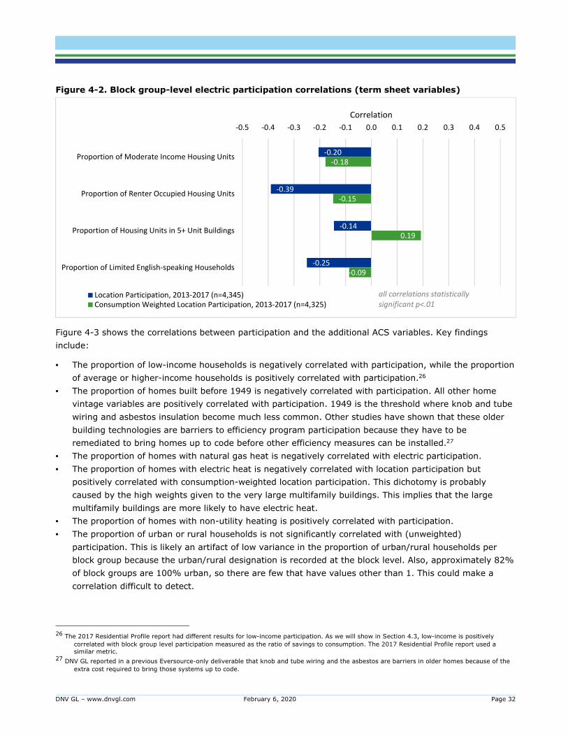
DNV GL – www.dnvgl.com February 6, 2020 Page 32
Figure 4-2. Block group-level electric participation correlations (term sheet variables)
Figure 4-3 shows the correlations between participation and the additional ACS variables. Key findings
include:
• The proportion of low-income households is negatively correlated with participation, while the proportion
of average or higher-income households is positively correlated with participation.26
• The proportion of homes built before 1949 is negatively correlated with participation. All other home
vintage variables are positively correlated with participation. 1949 is the threshold where knob and tube
wiring and asbestos insulation become much less common. Other studies have shown that these older
building technologies are barriers to efficiency program participation because they have to be
remediated to bring homes up to code before other efficiency measures can be installed.27
• The proportion of homes with natural gas heat is negatively correlated with electric participation.
• The proportion of homes with electric heat is negatively correlated with location participation but
positively correlated with consumption-weighted location participation. This dichotomy is probably
caused by the high weights given to the very large multifamily buildings. This implies that the large
multifamily buildings are more likely to have electric heat.
• The proportion of homes with non-utility heating is positively correlated with participation.
• The proportion of urban or rural households is not significantly correlated with (unweighted)
participation. This is likely an artifact of low variance in the proportion of urban/rural households per
block group because the urban/rural designation is recorded at the block level. Also, approximately 82%
of block groups are 100% urban, so there are few that have values other than 1. This could make a
correlation difficult to detect.
26 The 2017 Residential Profile report had different results for low-income participation. As we will show in Section 4.3, low-income is positively
correlated with block group level participation measured as the ratio of savings to consumption. The 2017 Residential Profile report used a
similar metric. 27 DNV GL reported in a previous Eversource-only deliverable that knob and tube wiring and the asbestos are barriers in older homes because of the
extra cost required to bring those systems up to code.
-0.20
-0.39
-0.14
-0.25
-0.18
-0.15
0.19
-0.09
-0.5 -0.4 -0.3 -0.2 -0.1 0.0 0.1 0.2 0.3 0.4 0.5
Proportion of Moderate Income Housing Units
Proportion of Renter Occupied Housing Units
Proportion of Housing Units in 5+ Unit Buildings
Proportion of Limited English-speaking Households
Correlation
Location Participation, 2013-2017 (n=4,345)
Consumption Weighted Location Participation, 2013-2017 (n=4,325)
all correlations statistically
significant p<.01

DNV GL – www.dnvgl.com February 6, 2020 Page 33
Figure 4-3. Block group-level electric participation correlations (extra ACS variables)
-0.36
-0.20
0.40
-0.34
0.34
-0.09
-0.13
0.18
0.02
-0.18
-0.18
0.23
-0.30
0.30
0.21
-0.16
0.03
0.05
-0.5 -0.4 -0.3 -0.2 -0.1 0.0 0.1 0.2 0.3 0.4 0.5
Proportion of Low Income Housing Units
Proportion of Moderate Income Housing Units
Proportion of Average or Higher Income
Housing Units
Proportion of Housing Units built before 1950
Proportion of Housing Units built in 1950 or
Later
Proportion of Households with Electric Heating
Proportion of Households with Gas Heating
Proportion of Households with Non-PA Heating
Proportion of Urban PA Households
Correlation
Location Participation, 2013-2017 (n=4,345)
Consumption Weighted Location Participation, 2013-2017 (n=4,325)
§ correlation NOT statistically significant at p<.05 or stronger

DNV GL – www.dnvgl.com February 6, 2020 Page 34
4.2.2 Electric participation block group-level models
Table 4-2 presents the electric block group model results for location and consumption-weighted location
participation. In both models, the relationships between most of the ACS variables and participation rate
remain similar to the zero-order correlations. This indicates that they each have independent effects on
participation. The exceptions are multifamily housing and limited English; the effects of which are different
in the models than in the zero-order correlations. This indicates that the effects of these two variables are
interacting with at least one of the other variables in the model.
Table 4-2. Initial electric block group models
Variable
Location Participation
Consumption Weighted
Participation
Coefficient Coefficient
Intercept 0.389 *** 0.393 ***
Proportion of Households at 56 - 85% of Statewide Median Income
-0.173 *** -0.164 ***
Proportion of Renter Occupied Housing Units -0.178 *** -0.221 ***
Proportion of Housing Units in 5+ Unit Buildings 0.081 *** 0.280 ***
Proportion of Limited English-speaking Households -0.027 0.027
*** p <.001; ** p < .01; * p < .1
There are three effects that change from the zero-order correlations when all the variables are included in
the models:
1. The strength of the effect of renting decreases.
2. The effect of limited English-speaking households becomes non-significant.28
3. The effect of multifamily housing becomes much more positive; so much so that it changes signs in the
location participation model.
Additional models (location participation: Table 4-3; consumption-weighted location participation: Table 4-4)
revealed that the renter variable is interacting with the multifamily and limited English variables. For both
types of participation, when the renter variable is absent from the model, the effects of multifamily housing
and limited English are similar to their zero-order correlations.
28 There is a sign change in the estimate for this variable for unweighted and location weighted participation. However, because neither value is
statistically significantly different than zero, DNV GL did not attempt to interpret the sign change.

DNV GL – www.dnvgl.com February 6, 2020 Page 35
Table 4-3. Electric location participation models with some variables removed
Variable
Without % Renter
Full Model
Coefficient Coefficient
Intercept 0.363 *** 0.389 ***
Proportion of Households at 56 - 85% of Statewide Median Income
-0.246 *** -0.173 ***
Proportion of Renter Occupied Housing Units -0.178 ***
Proportion of Housing Units in 5+ Unit Buildings -0.032 *** 0.081 ***
Proportion of Limited English-speaking Households -0.232 *** -0.027
*** p <.001; ** p < .01; * p < .1
Table 4-4. Electric consumption weighted location participation models renter variable
present/absent
Variable
Without % Renter
Full Model
Coefficient Coefficient
Intercept 0.362 *** 0.393 ***
Proportion of Households at 56 - 85% of Statewide Median Income
-0.255 *** -0.164 ***
Proportion of Renter Occupied Housing Units -0.221 ***
Proportion of Housing Units in 5+ Unit Buildings 0.139 *** 0.280 ***
Proportion of Limited English-speaking Households -0.228 *** 0.027
*** p <.001; ** p < .01; * p < .1
The interactions between renter status and the other two variables suggest that the effect of the other
variable (limited English or multifamily) is largely explained by the tendency of those groups to rent.
• Limited English is a barrier to participation mostly because of the tendency of that population to rent.
Limited English speakers tend to rent and not participate. Renters also tend to not participate. When the
tendency of renters to not participate is accounted for, we no longer see a significant effect of Limited
English. This is illustrated in the following pattern:
- Renter and limited English are positively correlated with each other (r=0.58) and both negatively
correlated with location participation (Renter r = -0.41; Limited English r= -0.26)
- In the model without Renter, Limited English remains a significant, negative predictor of
participation (Location coefficient=-0.232)
- When Renter is added to the model, renter is a significant, negative predictor of participation
(Location coefficient=-0.178) and limited English becomes non-significant (Location coefficient=-
0.027).
- Consumption-weighted participation has the same pattern, but with slightly different numeric
values.
Adding the other variables to the model, such as home construction vintage and heating fuel, did not cause
substantial changes to the results reported in this section (Table 4-5). The effects of multifamily and limited
English decreased slightly, but that is not unexpected when adding variables to the model that are known to
correlate with other variables.

DNV GL – www.dnvgl.com February 6, 2020 Page 36
Table 4-5. Electric block group model results with all variables29
Variable
Location Participation
Consumption-weighted Location
Participation
Coefficient Coefficient
Intercept 0.363 *** 0.372 ***
Proportion of Households at less than 56% of Statewide
Median Income -0.110 *** -0.120 ***
Proportion of Households at 56 - 85% of Statewide Median Income
-0.183 ***
-0.179 ***
Proportion of Renter Occupied Housing Units -0.089 *** -0.133 ***
Proportion of Housing Units in 5+ Unit Buildings 0.019 * 0.171 ***
Proportion of Limited English-speaking Households 0.009 0.053 *
Proportion of Households Built in 1949 or Earlier -0.070 *** -0.071 ***
Proportion of Households with Natural Gas Heating -0.036 *** -0.026 *
Proportion of Households with Electric Heating 0.027 * 0.165 ***
Proportion of Urban PA Households 0.089 *** 0.072 ***
4.2.3 Electric participation individual-level models
Data available at the individual account level (from all PAs) included renting, multifamily, construction date,
and urban/rural. In the enhanced individual-level models (Eversource only), we were able to also include the
effects of income and limited English.
As stated in the method section, we used account-level participation for the individual models because it is
at a grain similar to most of the independent variables. This type of participation reflects participation while
the resident lived in a particular house or apartment.
Correlations for individual-level data
Participation is negatively correlated with all four demographic variables available statewide30 (Table 4-6).
This means that people with moderate incomes, who rent, who live in multifamily housing, or who have
limited English skills are less likely to participate. Unlike the block group level models, these findings are not
subject to ecological fallacy and can be interpreted to indicate effects at an individual level. The individual-
level correlations are consistent with the block-group-level correlations in direction, though generally
weaker. Income and language information is not available at this data grain.
29 For variables that are perfectly collinear, meaning that there is a mutually exclusive relationship between them (e.g. urban and rural), one of the
variables must be dropped as there is no variation for the model to pick up. As an example, the proportion of rural PA households is 1 minus the
proportion of urban PA households. Because these two variables contain the same information and are linearly related to one another, they cannot
both be included in the same model. The variable dropped from the model can be interpreted as the reference case, meaning that the coefficient for
urban in this example is the impact of urban vs. rural. For these models, we dropped the proportion of households above 85% of the statewide
median income, the proportion of households built in 1950 or later, the proportion of households with non-utility heating, and the proportion of rural
households.
30 These results are for the combined statewide data set. We did not test results for individual PAs.

DNV GL – www.dnvgl.com February 6, 2020 Page 37
Table 4-6. Individual-level correlations – statewide electric
Variable Account
Participation, 2013-2017
Multifamily Renter Urban Pre-1950
Construction
Account Participation, 2013-2017
- -0.12 -0.20 -0.05 -0.11
Multifamily -0.12 - 0.32 0.09 0.09
Renter -0.20 0.32 - 0.18 0.30
Urban -0.05 0.09 0.18 - 0.15
Pre-1950 Construction
-0.11 0.09 0.30 0.15 -
Over 2 million observations per correlation. All correlations statistically significant p<0.001
Models for individual-level data
The individual-level models use binary logistic regression to predict a dependent variable that is set to 0 for
nonparticipating accounts and 1 for participating accounts. The coefficients of these models are logs of odd
ratios, which are difficult to interpret directly. The magnitude of the coefficient still reflects the relative
strength of the relationship. The sign indicates the direction of the relationship. Positive signs mean the
probability of participation increases as the independent variable increases and vice versa for negative
values.
Table 4-7 shows several model results predicting account participation for the variables that are available
statewide. These model results are consistent with the block group-level models. All of the independent
variables are negative predictors of participation. That is, renters are less likely to participate than non-
renters; people living in multifamily buildings are less likely to participate than those in other buildings, etc.
Because these models utilize individual-level variables, they can be interpreted as individual-level effects.
One effect is inconsistent with the block group level models. The main effect of multifamily residency in the
individual level models is the opposite of the effect in the block group models. In the block group models,
multifamily was a positive predictor of participation, especially when controlling for the effect of renting. The
difference in results is probably caused by the differences in the dependent variables in each model. In the
block group models, the dependent variable was location (or consumption weighted location) participation.
In the individual level models, the dependent variable is account participation. Location participation is
probably skewing the model outcomes. Because participation by any single unit in a multifamily building
creates a location participation value of 1, the more units in the building, the greater the probability that at
least one of them participated. In contrast, account participation is not affected by the number of units in a
building, and the model results indicate that individual units in multifamily buildings have a lower probability
of participating than those in non-multifamily buildings.

DNV GL – www.dnvgl.com February 6, 2020 Page 38
Table 4-7. Electric account participation models coefficients – statewide
Variable Model 1 Model 2 Model 3
Intercept -0.901 *** -0.900 *** -0.748 ***
Renter -0.850 *** -0.853 *** -0.753 ***
Resides in multifamily building
-1.018 *** -1.305 *** -1.204 ***
Renter * Multifamily1 0.303 *** 0.152 **
Resides in Urban block -0.051 ***
Pre-1950 construction -0.305 ***
*** p <.001; ** p < .01; * p < .1 1 Notation of variable a*b indicates an interaction term. A significant interaction means the effect of one variable depends on the level of the other
variable.
Similar to the block group-level model results, there is also a significant (although small) interaction
between renter and multifamily status in these models. Figure 4-4 illustrates the nature of that interaction
by graphing the expected probability of participation for the four combinations of renter and multifamily
status. For non-renters (Rent=0) and renters (Rent=1), multifamily has a negative effect on the probability
of participation. However, the negative effect of multifamily is not as strong for renters, which is indicated
by the smaller distance between the two columns in the renter category. It should be noted this relationship
is symmetrical: the negative effect of renting is less in multifamily buildings than it is in non-multifamily
buildings.
Figure 4-4. Renter*Multifamily interaction on electric account participation probability –
statewide
Correlations for enhanced individual-level data
In the enhanced individual-level data set, which primarily uses the Experian demographic data available only
for Eversource accounts, account participation is negatively correlated with multifamily, limited English,
moderate-income, pre-1950 construction, and urban (Table 4-8). These correlations are in the same
directions as the block-group and non-enhanced individual-level correlations. The effect for multifamily is
similar in magnitude, but the other effects are weaker than in the other data sets.
29%
15%
10%
6%
0%
5%
10%
15%
20%
25%
30%
35%
Rent 0 Rent 1
Pro
bability o
f Part
icip
ation
Multifamily 0 Multifamily 1

DNV GL – www.dnvgl.com February 6, 2020 Page 39
Table 4-8. Individual-level correlations – Enhanced electric data
Variable
Accou
nt
Parti
cip
ati
on
,
20
13
-2
01
7
Ren
ter
Mu
ltif
am
ily
Lim
ited
En
gli
sh
Low
In
co
me
Mod
erate
In
com
e
Avg
or H
igh
er
In
com
e
Pre-1
95
0
Con
str
ucti
on
Urb
an
Account Participation, 2013-2017
-
-0.14 -0.19 -0.04 -0.04 -0.04 0.06 -0.11 -0.05
Renter -0.14
- 0.41 0.18 0.30 -0.01 -0.23 0.20 0.11
Multifamily -0.19 0.41
- 0.14 0.19 0.01 -0.16 0.26 0.17
Limited English -0.04 0.18 0.14
- 0.09 -0.01 -0.06 0.08 0.09
Low Income -0.04 0.30 0.19 0.09
- -0.32 -0.50 0.08 0.05
Moderate Income -0.04 -0.01 0.01 -0.01 -0.32
- -0.66 0.02 -0.05
Average or Higher Income
0.06 -0.23 -0.16 -0.06 -0.50 -0.66
- -0.08 0.00
Pre-1950 Construction
-0.11 0.20 0.26 0.08 0.08 0.02 -0.08
- 0.15
Urban -0.05 0.11 0.17 0.09 0.05 -0.05 0.00 0.15
- Approximately 1 million observations per correlation. All correlations statistically significant p<.001 except for Average or higher income and urban.
Models for enhanced individual-level data
The results of the enhanced models are very similar to those for the individual-level data. Renter and
multifamily are both negatively associated with participation (Table 4-9).
The enhanced models include a variable for moderate-income that the individual-level models cannot. As
observed in the correlations and in the block group-level models, moderate-income is negatively associated
with participation. The enhanced models also include a variable for limited English that is negatively
associated with participation.

DNV GL – www.dnvgl.com February 6, 2020 Page 40
Table 4-9. Electric account participation models coefficients – enhanced data
Variable Model 1 Model 2 Model 3 Model 4 Model 5
Intercept -0.723 *** -0.658 *** -0.649 *** -0.650 *** -0.590 ***
Experian Low Income
-0.059 ***
Experian Moderate
Income -0.149 *** -0.158 *** -0.155 *** -0.156 *** -0.166 ***
Experian Renter -0.524 *** -0.646 *** -0.596 *** -0.552 ***
Experian resides in
multifamily building
-1.017 *** -0.781 *** -0.843 *** -0.782 *** -0.770 ***
Experian limited English
-0.096 *** -0.057 *** -0.058 *** -0.137 *** -0.083 ***
Resides in Urban Block
0.030 **
Pre-1950
construction -0.159 ***
Experian Renter * Multifamily1
0.259 ***
Experian Renter * Limited English1
0.317 ***
*** p <.001; ** p < .01; * p < .1
1 Notation of variable a*b indicates an interaction term. A significant interaction means the effect of one variable depends on the level of the other
variable.
The interaction between renting and limited English is significant in the enhanced individual-level models.
Figure 4-5 illustrates the nature of that interaction by graphing the expected probability of participation for
the four combinations of renter and limited English status. For non-renters (Rent=0), limited English has a
positive effect on the probability of participation. However, the relationship switches for renters (Rent=1),
such that limited English decreases the probability of participation. Despite being statistically significant, it is
difficult to imagine a real-life scenario that can explain this relationship. It is most likely a statistical artifact.
Figure 4-5. Renter*Limited English interaction on electric account participation probability –
enhanced data
31%
15%
26%
16%
0%
5%
10%
15%
20%
25%
30%
35%
Rent 0 Rent 1
Pro
bability o
f Part
icip
ation
Limited English 0 Limited English 1

DNV GL – www.dnvgl.com February 6, 2020 Page 41
There is also a statistically significant interaction between renter and multifamily in the enhanced models.
Figure 4-6 illustrates the nature of that relationship. It is very similar to the relationship observed in the
individual-level models.
Figure 4-6. Renter*Multifamily interaction on electric account participation probability –
enhanced data
4.3 Electric savings/consumption findings
4.3.1 Block group electric analysis
Figure 4-7 shows the zero-order correlations between the electric participation metrics, income, the term
sheet variables, and several other ACS variables at the block group level. Location participation correlations
are repeated here for the sake of contrast. As Figure 4-7 shows, correlations change for four key variables
depending on how participation is measured. Low income, renter, multifamily, and limited English correlate
negatively with location participation. By contrast, these variables correlate positively with the
savings/consumption metric. This pattern suggests that while the electric PAs might have lower participation
in block groups with more low income, renters, multifamily, and limited English households in terms of
number of participants, those participants have a relatively high depth of savings (and accordingly, a high
savings-to-consumption ratio).
33%
21%
18%
13%
0%
5%
10%
15%
20%
25%
30%
35%
Rent 0 Rent 1
Pro
ba
bil
ity
of
Pa
rtic
ipa
tio
n
Multifamily 0 Multifamily 1

DNV GL – www.dnvgl.com February 6, 2020 Page 42
Figure 4-7. Block group electric correlations
-0.36
-0.20
0.40
-0.39
-0.14
-0.25
-0.34
0.34
-0.09
-0.13
0.18
0.02
-0.18
-0.18
0.23
-0.15
0.19
-0.09
-0.30
0.30
0.21
-0.16
0.03
0.05
0.07
-0.11
-0.02
0.01
0.14
0.08
-0.17
0.17
0.12
-0.07
0.00
0.01
-0.5 -0.4 -0.3 -0.2 -0.1 0.0 0.1 0.2 0.3 0.4 0.5
Proportion of Low Income Housing Units
Proportion of Moderate Income Housing Units
Proportion of Average or Higher Income HousingUnits
Proportion of Renter Occupied Housing Units
Proportion of Housing Units in 5+ Unit Buildings
Proportion of Limited English-speakingHouseholds
Proportion of Housing Units built before 1950
Proportion of Housing Units built in 1950 or Later
Proportion of Households with Electric Heating
Proportion of Households with Gas Heating
Proportion of Households with Non-PA Heating
Proportion of Urban PA Households
Correlation
Location Participation, 2013-2017 (n=4,345)
Consumption Weighted Location Participation, 2013-2017 (n=4,325)
Savings over Average Consumption, 2013-2017 (n=4,338)
§ correlation NOT statistically significant at p<.05 or stronger
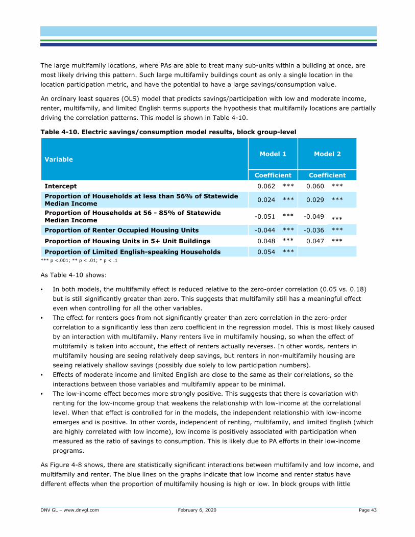
DNV GL – www.dnvgl.com February 6, 2020 Page 43
The large multifamily locations, where PAs are able to treat many sub-units within a building at once, are
most likely driving this pattern. Such large multifamily buildings count as only a single location in the
location participation metric, and have the potential to have a large savings/consumption value.
An ordinary least squares (OLS) model that predicts savings/participation with low and moderate income,
renter, multifamily, and limited English terms supports the hypothesis that multifamily locations are partially
driving the correlation patterns. This model is shown in Table 4-10.
Table 4-10. Electric savings/consumption model results, block group-level
Variable Model 1 Model 2
Coefficient Coefficient
Intercept 0.062 *** 0.060 ***
Proportion of Households at less than 56% of Statewide Median Income
0.024 *** 0.029 ***
Proportion of Households at 56 - 85% of Statewide Median Income
-0.051 *** -0.049 ***
Proportion of Renter Occupied Housing Units -0.044 *** -0.036 ***
Proportion of Housing Units in 5+ Unit Buildings 0.048 *** 0.047 ***
Proportion of Limited English-speaking Households 0.054 ***
*** p <.001; ** p < .01; * p < .1
As Table 4-10 shows:
• In both models, the multifamily effect is reduced relative to the zero-order correlation (0.05 vs. 0.18)
but is still significantly greater than zero. This suggests that multifamily still has a meaningful effect
even when controlling for all the other variables.
• The effect for renters goes from not significantly greater than zero correlation in the zero-order
correlation to a significantly less than zero coefficient in the regression model. This is most likely caused
by an interaction with multifamily. Many renters live in multifamily housing, so when the effect of
multifamily is taken into account, the effect of renters actually reverses. In other words, renters in
multifamily housing are seeing relatively deep savings, but renters in non-multifamily housing are
seeing relatively shallow savings (possibly due solely to low participation numbers).
• Effects of moderate income and limited English are close to the same as their correlations, so the
interactions between those variables and multifamily appear to be minimal.
• The low-income effect becomes more strongly positive. This suggests that there is covariation with
renting for the low-income group that weakens the relationship with low-income at the correlational
level. When that effect is controlled for in the models, the independent relationship with low-income
emerges and is positive. In other words, independent of renting, multifamily, and limited English (which
are highly correlated with low income), low income is positively associated with participation when
measured as the ratio of savings to consumption. This is likely due to PA efforts in their low-income
programs.
As Figure 4-8 shows, there are statistically significant interactions between multifamily and low income, and
multifamily and renter. The blue lines on the graphs indicate that low income and renter status have
different effects when the proportion of multifamily housing is high or low. In block groups with little

DNV GL – www.dnvgl.com February 6, 2020 Page 44
multifamily housing (dark blue line), we expect participation to decrease when there are more renters
and/or more low income households. However, in block groups with a lot of multifamily housing (light blue
lines), we expect participation to increase with when there are more renters and/or more low income
households. As multifamily increases, so do the expected participation rates for low income or renters
increases. These interactions provide additional evidence that something is happening in multifamily
buildings or areas that changes the effect of the other variables. PAs achieving deeper savings in multifamily
buildings, particularly low income multifamily buildings, could explain these interactions.
Figure 4-8. Multifamily interactions with low income and renter
0%
5%
10%
15%
20%
LowIncome
0%
LowIncome50%
LowIncome100%E
xpecte
d P
art
icip
ation
Rate
s
MF 0% MF 50% MF 100%
0%
5%
10%
15%
20%
Rent 0% Rent 50% Rent 100%Expecte
d P
art
icip
ation
Rate
s
MF 0% MF 50% MF 100%

DNV GL – www.dnvgl.com February 6, 2020 Page 45
4.3.2 Individual-level electric analysis – Statewide
Figure 4-9 shows the statewide, zero-order, account-level correlations between the electric participation
metrics, multifamily, renter, urban, and pre-1950 construction (other characteristics are not available at the
account level). Account participation correlations are repeated here for the sake of contrast. Unlike the
block-group level correlations, the account-level correlations with savings/consumption go in the same
direction as for account participation.
Figure 4-9. Individual-level correlations with savings over consumption, statewide electric
Table 4-11 shows results for models that DNV GL used to isolate the effects of the different variables
independently of the other variables. In all three models, the coefficients go in the same direction and are
approximately the same magnitude as the zero-order correlations. This means that the covariation between
the various characteristics (e.g., multifamily residents tend to rent) does not mask or substantially change
the effects of any singular characteristic. There is a statistically significant interaction between renter and
multifamily that indicates there is a significant overlap in the effects of each variable. However, that overlap
is not enough to change overall (correlation) versus independent (model coefficient) effect of either variable.
Table 4-11. Individual-level savings over consumption models, statewide electric
Variable Model 1 Model 2 Model 3
Intercept 0.048 *** 0.048 *** 0.053 ***
Renter -0.020 *** -0.020 *** -0.017 ***
Resides in multifamily building -0.015 *** -0.027 *** -0.024 ***
Renter * Multifamily 1 0.012 *** 0.008 ***
Resides in Urban block -0.002 ***
Pre-1950 construction -0.008 ***
*** p <.001; ** p < .01; * p < .1
1 Notation of variable a*b indicates an interaction term. A significant interaction means the effect of one variable depends on the level of the other
variable.
-0.12
-0.20
-0.05
-0.11
-0.07
-0.12
-0.03
-0.07
-0.25 -0.15 -0.05 0.05 0.15 0.25
Multifamily
Renter
Urban
Pre-1950 Construction
Correlation
Account Participation, 2013-2017
Savings/ Avg. Consumption, 2013-2017
all correlations statistically significant p<.01

DNV GL – www.dnvgl.com February 6, 2020 Page 46
4.3.3 Individual-level electric analysis – Enhanced
Figure 4-10 shows the Eversource-only, enhanced data, zero-order account-level correlations between the
electric participation metrics, income, renter, multifamily, limited English, construction vintage, and urban.
Account participation correlations are repeated here for the sake of contrast. Unlike the block-group level
correlations and similar to the statewide account-level correlations, the enhanced account-level correlations
with savings/consumption go in the same direction as for enhanced account participation.
Figure 4-10. Individual-level correlations with savings over consumption, enhanced electric
Table 4-12 shows results for models that DNV GL used to isolate the effects of the different variables
independently of the other variables. Except for low and moderate income, the coefficients for each of the
variables are similar to the zero-order correlations. This means the overall effect of the variable (correlation)
is similar to the independent effect when controlling for the covariation with the other characteristics
(coefficients). For low and moderate income, the coefficients in the models shift, which indicates that the
overall effect of those variables is partially affected by overlaps with the other characteristics.
-0.04
-0.04
0.06
-0.14
-0.19
-0.04
-0.11
-0.05
-0.01
-0.01
0.02
-0.09
-0.12
-0.03
-0.07
-0.03
-0.20 -0.10 0.00 0.10 0.20
Low Income
Moderate Income
Average or Higher Income
Renter
Multifamily
Limited English
Pre-1950 Construction
Urban
Correlation
Account Participation, 2013-2017
Savings/ Avg. Consumption, 2013-2017
all correlations statistically significant p<.01
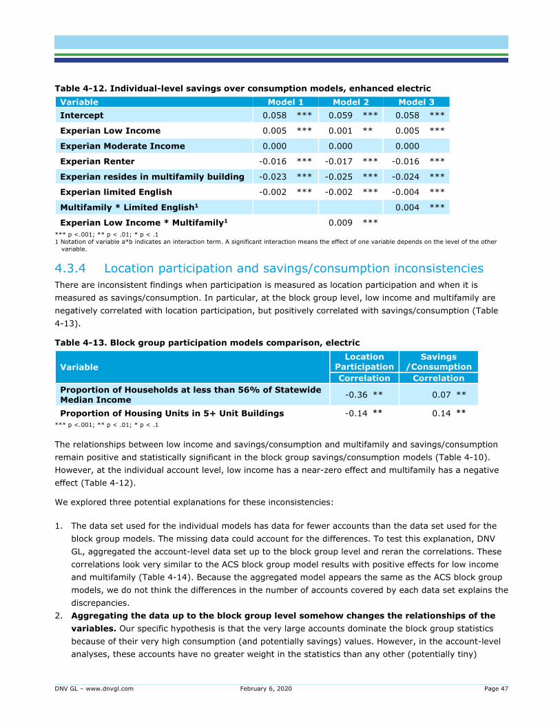
DNV GL – www.dnvgl.com February 6, 2020 Page 47
Table 4-12. Individual-level savings over consumption models, enhanced electric
Variable Model 1 Model 2 Model 3
Intercept 0.058 *** 0.059 *** 0.058 ***
Experian Low Income 0.005 *** 0.001 ** 0.005 ***
Experian Moderate Income 0.000 0.000 0.000
Experian Renter -0.016 *** -0.017 *** -0.016 ***
Experian resides in multifamily building -0.023 *** -0.025 *** -0.024 ***
Experian limited English -0.002 *** -0.002 *** -0.004 ***
Multifamily * Limited English1 0.004 ***
Experian Low Income * Multifamily1 0.009 ***
*** p <.001; ** p < .01; * p < .1
1 Notation of variable a*b indicates an interaction term. A significant interaction means the effect of one variable depends on the level of the other
variable.
4.3.4 Location participation and savings/consumption inconsistencies
There are inconsistent findings when participation is measured as location participation and when it is
measured as savings/consumption. In particular, at the block group level, low income and multifamily are
negatively correlated with location participation, but positively correlated with savings/consumption (Table
4-13).
Table 4-13. Block group participation models comparison, electric
Variable
Location Participation
Savings /Consumption
Correlation Correlation
Proportion of Households at less than 56% of Statewide Median Income
-0.36 ** 0.07 **
Proportion of Housing Units in 5+ Unit Buildings -0.14 ** 0.14 ** *** p <.001; ** p < .01; * p < .1
The relationships between low income and savings/consumption and multifamily and savings/consumption
remain positive and statistically significant in the block group savings/consumption models (Table 4-10).
However, at the individual account level, low income has a near-zero effect and multifamily has a negative
effect (Table 4-12).
We explored three potential explanations for these inconsistencies:
1. The data set used for the individual models has data for fewer accounts than the data set used for the
block group models. The missing data could account for the differences. To test this explanation, DNV
GL, aggregated the account-level data set up to the block group level and reran the correlations. These
correlations look very similar to the ACS block group model results with positive effects for low income
and multifamily (Table 4-14). Because the aggregated model appears the same as the ACS block group
models, we do not think the differences in the number of accounts covered by each data set explains the
discrepancies.
2. Aggregating the data up to the block group level somehow changes the relationships of the
variables. Our specific hypothesis is that the very large accounts dominate the block group statistics
because of their very high consumption (and potentially savings) values. However, in the account-level
analyses, these accounts have no greater weight in the statistics than any other (potentially tiny)
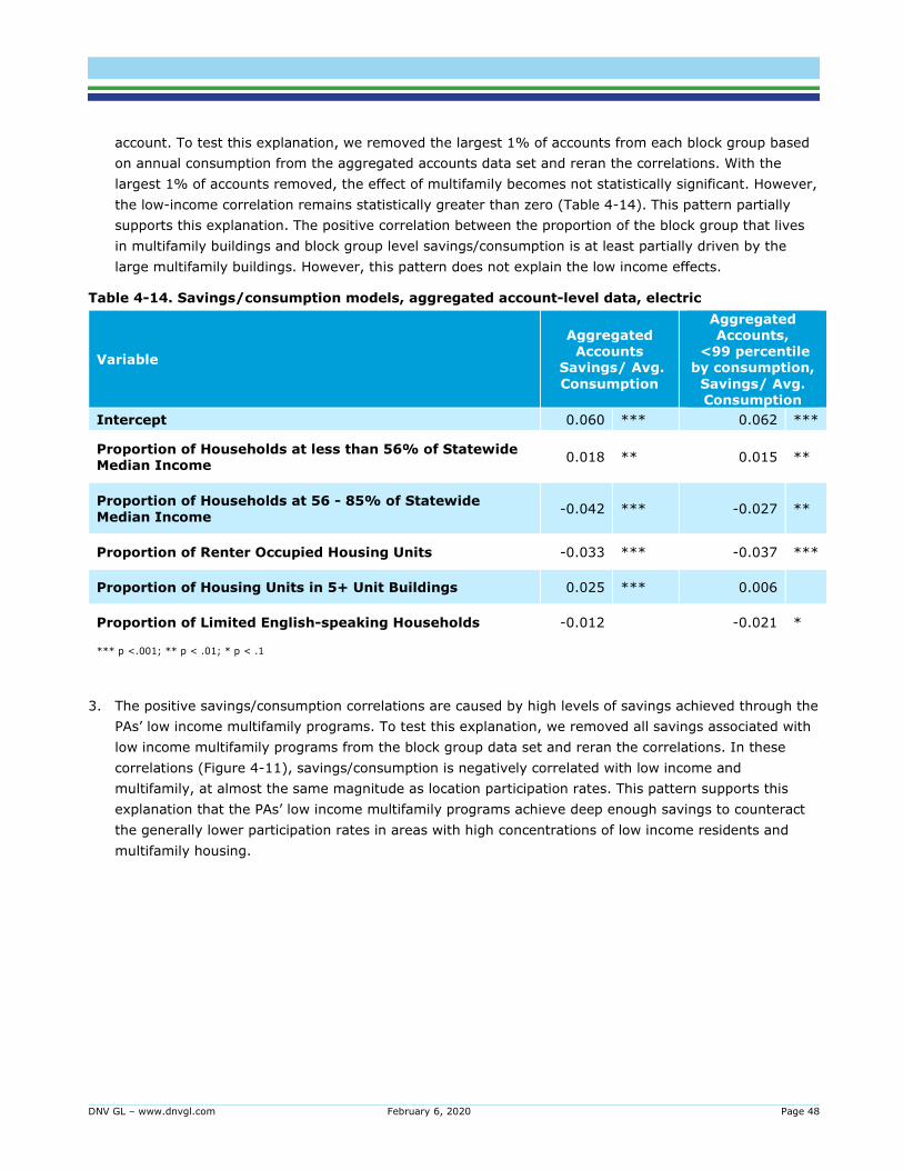
DNV GL – www.dnvgl.com February 6, 2020 Page 48
account. To test this explanation, we removed the largest 1% of accounts from each block group based
on annual consumption from the aggregated accounts data set and reran the correlations. With the
largest 1% of accounts removed, the effect of multifamily becomes not statistically significant. However,
the low-income correlation remains statistically greater than zero (Table 4-14). This pattern partially
supports this explanation. The positive correlation between the proportion of the block group that lives
in multifamily buildings and block group level savings/consumption is at least partially driven by the
large multifamily buildings. However, this pattern does not explain the low income effects.
Table 4-14. Savings/consumption models, aggregated account-level data, electric
Variable
Aggregated Accounts
Savings/ Avg.
Consumption
Aggregated Accounts,
<99 percentile by consumption,
Savings/ Avg. Consumption
Intercept 0.060 *** 0.062 ***
Proportion of Households at less than 56% of Statewide Median Income
0.018 ** 0.015 **
Proportion of Households at 56 - 85% of Statewide
Median Income -0.042 *** -0.027 **
Proportion of Renter Occupied Housing Units -0.033 *** -0.037 ***
Proportion of Housing Units in 5+ Unit Buildings 0.025 *** 0.006
Proportion of Limited English-speaking Households -0.012 -0.021 *
*** p <.001; ** p < .01; * p < .1
3. The positive savings/consumption correlations are caused by high levels of savings achieved through the
PAs’ low income multifamily programs. To test this explanation, we removed all savings associated with
low income multifamily programs from the block group data set and reran the correlations. In these
correlations (Figure 4-11), savings/consumption is negatively correlated with low income and
multifamily, at almost the same magnitude as location participation rates. This pattern supports this
explanation that the PAs’ low income multifamily programs achieve deep enough savings to counteract
the generally lower participation rates in areas with high concentrations of low income residents and
multifamily housing.

DNV GL – www.dnvgl.com February 6, 2020 Page 49
Figure 4-11. Block group correlations, electric, no LIMF savings
-0.46
-0.19
0.50
-0.49
-0.23
-0.35
-0.35
0.35
-0.17
-0.13
0.23
0.00
-0.16
-0.18
0.22
-0.14
0.20
-0.08
-0.30
0.30
0.22
-0.16
0.03
0.05
-0.37
-0.12
0.38
-0.41
-0.21
-0.30
-0.32
0.32
-0.16
-0.12
0.21
-0.09
-0.5 -0.4 -0.3 -0.2 -0.1 0.0 0.1 0.2 0.3 0.4 0.5
Proportion of Low Income Housing Units
Proportion of Moderate Income Housing Units
Proportion of Average or Higher Income Housing
Units
Proportion of Renter Occupied Housing Units
Proportion of Housing Units in 5+ Unit Buildings
Proportion of Limited English-speaking
Households
Proportion of Housing Units built before 1950
Proportion of Housing Units built in 1950 or Later
Proportion of Households with Electric Heating
Proportion of Households with Gas Heating
Proportion of Households with Non-PA Heating
Proportion of Urban PA Households
Correlation
Location Participation, 2013-2017 (n=4,337)
Consumption Weighted Location Participation, 2013-2017 (n=4,329)
Savings over Average Consumption, 2013-2017 (n=4,348)
§ correlation NOT statistically
significant at p<.05 or stronger

DNV GL – www.dnvgl.com February 6, 2020 Page 50
4.4 Gas location participation findings
4.4.1 ACS variable correlations with gas participation
Figure 4-12 presents the correlations between gas location and gas consumption-weighted location
participation and the primary ACS variables. Correlations between these variables are negative and
statistically significant. This indicates that block groups with higher concentrations of the term sheet
variables have lower participation rates.
Figure 4-12. Block group-level gas participation correlations (term sheet variables)
Figure 4-13 shows the correlations between gas participation and the additional ACS variables. Key findings
include:
• The proportion of low-income households is negatively correlated with participation, while the proportion
of high-income households is positively correlated with participation.
• The proportion of homes built before 1949 is negatively correlated with participation. All other home
vintage variables are positively correlated with participation. 1949 is the threshold where knob and tube
wiring and asbestos insulation become much less common. Other studies have shown that these older
building technologies are barriers to efficiency program participation because they have to remediated to
bring homes up to code before other efficiency measures can be installed.31
• The proportion of homes with natural gas heat or electric heat is negatively correlated with gas program
participation. In contrast, the proportion of homes with non-utility heat is positively correlated with gas
program participation. DNV GL cannot account for this pattern at this time.
31 DNV GL reported in a previous Eversource-only deliverable that knob and tube wiring and the asbestos are barriers in older homes because of the
extra cost required to bring those systems up to code.
-0.24
-0.46
-0.20
-0.33
-0.23
-0.41
-0.08
-0.34
-0.5 -0.4 -0.3 -0.2 -0.1 0.0 0.1 0.2 0.3 0.4 0.5
Proportion of Moderate Income Housing Units
Proportion of Renter Occupied Housing Units
Proportion of Housing Units in 5+ Unit Buildings
Proportion of Limited English-speakingHouseholds
Correlation
Location Participation, 2013-2017 (n=4,127) all correlations statistically
significant p<.01

DNV GL – www.dnvgl.com February 6, 2020 Page 51
• The proportion of urban and rural households is significantly correlated with participation. Residents in
block groups with a greater proportion of urban blocks are less likely to participate in gas programs than
residents in block groups with a lower proportion of urban blocks. This finding should be interpreted with
caution because of the skew towards urban blocks in Massachusetts.
Figure 4-13. Block group-level gas participation correlations (extra ACS variables)
4.4.2 Gas participation block group-level models
Table 4-15 presents the gas block group model results for location and gas consumption-weighted
participation variables. In both models, the relationships between the ACS variables and participation rate
remain similar to the zero-order correlations. This indicates that they each have independent effects on
participation. The exceptions are multifamily housing and limited English; the effects of which are different
in the models than in the zero-order correlations. This indicates these variables are interacting with at least
one of the other variables in the model.
-0.48
-0.24
0.52
-0.31
0.31
-0.18
-0.11
0.24
-0.10
-0.46
-0.23
0.51
-0.33
0.33
-0.09
-0.16
0.22
-0.11
-0.6 -0.4 -0.2 0.0 0.2 0.4 0.6
Proportion of Low Income Housing Units
Proportion of Moderate Income Housing Units
Proportion of Average or Higher Income
Housing Units
Proportion of Housing Units built before 1950
Proportion of Housing Units built in 1950 orLater
Proportion of Households with Electric Heating
Proportion of Households with Gas Heating
Proportion of Households with Non-PA Heating
Proportion of Urban PA Households
Correlation
Location Participation, 2013-2017 (n=4,133)
Consumption Weighted Location Participation, 2013-2017 (n=4,053)
§ correlation NOT statistically significant at p<.05 or stronger

DNV GL – www.dnvgl.com February 6, 2020 Page 52
Table 4-15. Initial gas block group models
Variable
Location Participation
Consumption Weighted
Participation
Estimate Estimate
Intercept 0.339*** 0.358***
Proportion of Households at 56 - 85% of Statewide Median Income
-0.227*** -0.217***
Proportion of Renter Occupied Housing Units -0.198*** -0.215***
Proportion of Housing Units in 5+ Unit Buildings 0.082*** 0.163***
Proportion of Limited English-speaking Households -0.105*** -0.197*** *** p <.001; ** p < .01; * p < .1

DNV GL – www.dnvgl.com February 6, 2020 Page 53
There are three effects that change from the zero-order correlations when all the variables are added
together into the models:
1. The effect of renting remains statistically significant but is much weaker than the zero-order correlation.
2. The effect of limited English-speaking households remains statistically significant but is much weaker
than the zero-order correlation.
3. The effect of multifamily housing changes sign from a negative correlation to a positive regression
coefficient.
Additional models (location participation: Table 4-16; consumption-weighted location participation: Table
4-17) revealed that the renter variable is interacting with the multifamily and limited English variables. For
both types of participation, when the renter variable is absent from the model, the effects of multifamily
housing and limited English are similar to their zero-order correlations.
Table 4-16. Gas location participation models; renter variable present/absent
Variable
Without % Rental
Full Model
Estimate Estimate
Intercept 0.313*** 0.339***
Proportion of Households at 56 - 85% of Statewide Median
Income -0.315*** -0.227***
Proportion of Renter Occupied Housing Units -0.198***
Proportion of Housing Units in 5+ Unit Buildings -0.046*** 0.082***
Proportion of Limited English-speaking Households -0.334*** -0.105*** *** p <.001; ** p < .01; * p < .1
Table 4-17. Gas consumption weighted location participation models renter variable
present/absent
Variable
Without % Renter
Full Model
Coefficient Coefficient
Intercept 0.331 *** 0.358 ***
Proportion of Households at 56 - 85% of Statewide Median Income
-0.317 *** -0.217 ***
Proportion of Renter Occupied Housing Units -0.215 ***
Proportion of Housing Units in 5+ Unit Buildings 0.024 ** 0.163 ***
Proportion of Limited English-speaking Households -0.448 *** -0.197 ***
*** p <.001; ** p < .01; * p < .1
The interpretation of these interactions is similar to that for electric participation. The interactions between
renter and the other two variables suggest that the effect of the other variable (limited English or
multifamily) is partially explained by those groups’ tendency to also rent.
• Limited English is a barrier to participation partially because of the tendency of that population to rent.
Limited English speakers tend to rent and not participate. Renters also tend to not participate. When the
tendency of renters to not participate is accounted for, the strength of the effect of Limited English
decreases by about half. The fact that Limited English remains a significant predictor indicates that
DNV GL – www.dnvgl.com February 6, 2020 Page 54
renting only partially explains the effect of Limited English. Even after the tendency of limited English
speakers to rent is accounted for, there still appears to be a statistically significant language barrier.
This is illustrated in the following pattern:
- Renter and limited English are positively correlated with each other (r=0.58) and both negatively
correlated with location participation (Renter r = -0.46; Limited English r= -0.33)
- In the model without Renter, Limited English remains a significant, negative predictor of
participation (Location coefficient=-0.448)
- When Renter is added to the model, renter is a significant, negative predictor of participation
(Location coefficient=-0.215) and limited English remains significant, but has a lesser magnitude
(Location coefficient=-0.197).
- Consumption-weighted participation has the same pattern, but with slightly different numeric
values.
• Multifamily housing is a barrier to participation mostly because of the tendency of that population to
rent; absent the association with renting, multifamily locations are positively associated with location
participation. A similar pattern applies to multifamily housing and renting. People living in multifamily
housing tend to rent and not participate. Renters tend to not participate. When we account for the
nonparticipation tendency of renters, the effect of Multifamily actually becomes slightly (but statistically
significantly) positive. In the case of consumption-weighted participation, Multifamily starts out
positively associated with participation and renting. Renting is still negatively associated with
participation, so it decreases the Multifamily effect. When the effect of Renting is removed from
Multifamily, the positive effect of Multifamily becomes stronger.32
A graph of the expected values from the regression model illustrates this relationship (Figure 4-14). The
positive effect of multifamily is evident in the vertical separation between the lines. That vertical
separation decreases as the proportion of renters increases.
32 The amplification of the positive effect of Multifamily in the location weighted model is caused by the weighting. Large multifamily buildings have a
higher chance of participation both because they are targeted more aggressively by the PAs and because there are more residents there and
therefore more chance for at least one of them to participate. The weighting makes it so that the whole building gets credit even if only one unit
participates.

DNV GL – www.dnvgl.com February 6, 2020 Page 55
Figure 4-14. Expected gas location participation rate (renter * multifamily)
Adding the other variables to the model, such as home construction vintage and heating fuel, did not cause
significant changes to the results reported in this section (Table 4-18). The direction of all coefficients stayed
the same. The strengths of the coefficients decreased to some degree, but that is expected when adding
variables with covariance to a model.
Table 4-18. Gas block group model results with all variables
Variable
Location
Participation
Consumption-weighted
Location Participation
Coefficient Coefficient
Intercept 0.363 *** 0.411 ***
Proportion of Households at less than 56% of Statewide Median Income
-0.260 *** -0.259 ***
Proportion of Households at 56 - 85% of Statewide Median Income
-0.199 *** -0.243 ***
Proportion of Renter Occupied Housing Units -0.084 *** -0.064 ***
Proportion of Housing Units in 5+ Unit Buildings 0.047 *** 0.116 ***
Proportion of Limited English-speaking Households -0.032 -0.112 ***
Proportion of Households Built in 1949 or Earlier -0.043 *** -0.060 ***
Proportion of Households with Natural Gas Heating 0.006 -0.001
Proportion of Households with Electric Heating 0.017 0.017
Proportion of Urban PA Households 0.014 -0.003
0%
5%
10%
15%
20%
25%
30%
35%
40%
45%
50%
Rent 0% Rent 50% Rent 100%
Expecte
d P
art
icip
ation R
ate
s
MF 0% MF 50% MF 100%
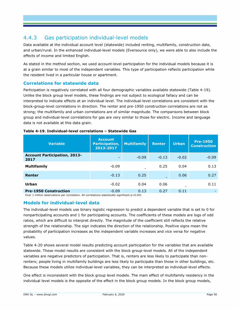
DNV GL – www.dnvgl.com February 6, 2020 Page 56
4.4.3 Gas participation individual-level models
Data available at the individual account level (statewide) included renting, multifamily, construction date,
and urban/rural. In the enhanced individual-level models (Eversource only), we were able to also include the
effects of income and limited English.
As stated in the method section, we used account-level participation for the individual models because it is
at a grain similar to most of the independent variables. This type of participation reflects participation while
the resident lived in a particular house or apartment.
Correlations for statewide data
Participation is negatively correlated with all four demographic variables available statewide (Table 4-19).
Unlike the block group level models, these findings are not subject to ecological fallacy and can be
interpreted to indicate effects at an individual level. The individual-level correlations are consistent with the
block-group-level correlations in direction. The renter and pre-1950 construction correlations are not as
strong; the multifamily and urban correlations are of similar magnitude. The comparisons between block
group and individual-level correlations for gas are very similar to those for electric. Income and language
data is not available at this data grain.
Table 4-19. Individual-level correlations – Statewide Gas
Variable Account
Participation, 2013-2017
Multifamily Renter Urban Pre-1950
Construction
Account Participation, 2013-
2017 - -0.09 -0.13 -0.02 -0.09
Multifamily -0.09
- 0.25 0.04 0.13
Renter -0.13 0.25
- 0.06 0.27
Urban -0.02 0.04 0.06
- 0.11
Pre-1950 Construction -0.09 0.13 0.27 0.11 - Over 1 million observations per correlation. All correlations statistically significant p<0.001
Models for individual-level data
The individual-level models use binary logistic regression to predict a dependent variable that is set to 0 for
nonparticipating accounts and 1 for participating accounts. The coefficients of these models are logs of odd
ratios, which are difficult to interpret directly. The magnitude of the coefficient still reflects the relative
strength of the relationship. The sign indicates the direction of the relationship. Positive signs mean the
probability of participation increases as the independent variable increases and vice versa for negative
values.
Table 4-20 shows several model results predicting account participation for the variables that are available
statewide. These model results are consistent with the block group-level models. All of the independent
variables are negative predictors of participation. That is, renters are less likely to participate than non-
renters; people living in multifamily buildings are less likely to participate than those in other buildings, etc.
Because these models utilize individual-level variables, they can be interpreted as individual-level effects.
One effect is inconsistent with the block group level models. The main effect of multifamily residency in the
individual level models is the opposite of the effect in the block group models. In the block group models,
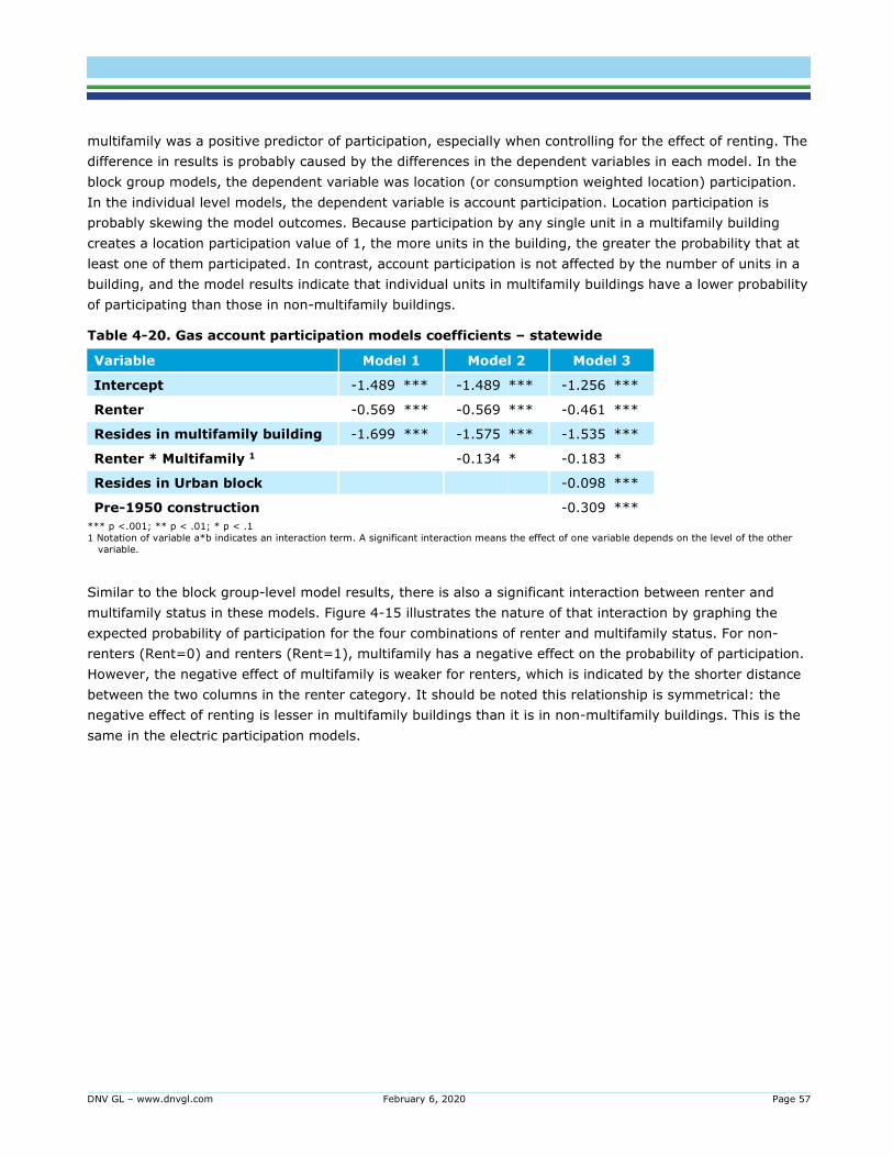
DNV GL – www.dnvgl.com February 6, 2020 Page 57
multifamily was a positive predictor of participation, especially when controlling for the effect of renting. The
difference in results is probably caused by the differences in the dependent variables in each model. In the
block group models, the dependent variable was location (or consumption weighted location) participation.
In the individual level models, the dependent variable is account participation. Location participation is
probably skewing the model outcomes. Because participation by any single unit in a multifamily building
creates a location participation value of 1, the more units in the building, the greater the probability that at
least one of them participated. In contrast, account participation is not affected by the number of units in a
building, and the model results indicate that individual units in multifamily buildings have a lower probability
of participating than those in non-multifamily buildings.
Table 4-20. Gas account participation models coefficients – statewide
Variable Model 1 Model 2 Model 3
Intercept -1.489 *** -1.489 *** -1.256 ***
Renter -0.569 *** -0.569 *** -0.461 ***
Resides in multifamily building -1.699 *** -1.575 *** -1.535 ***
Renter * Multifamily 1 -0.134 * -0.183 *
Resides in Urban block -0.098 ***
Pre-1950 construction -0.309 ***
*** p <.001; ** p < .01; * p < .1
1 Notation of variable a*b indicates an interaction term. A significant interaction means the effect of one variable depends on the level of the other
variable.
Similar to the block group-level model results, there is also a significant interaction between renter and
multifamily status in these models. Figure 4-15 illustrates the nature of that interaction by graphing the
expected probability of participation for the four combinations of renter and multifamily status. For non-
renters (Rent=0) and renters (Rent=1), multifamily has a negative effect on the probability of participation.
However, the negative effect of multifamily is weaker for renters, which is indicated by the shorter distance
between the two columns in the renter category. It should be noted this relationship is symmetrical: the
negative effect of renting is lesser in multifamily buildings than it is in non-multifamily buildings. This is the
same in the electric participation models.

DNV GL – www.dnvgl.com February 6, 2020 Page 58
Figure 4-15. Renter* multifamily interaction on gas account participation probability – statewide
Correlations for enhanced individual-level data
In the enhanced individual-level data set, which primarily uses the Experian demographic data available only
for Eversource accounts, account participation is negatively correlated with multifamily, limited English,
moderate-income, pre-1950 construction, and urban (Table 4-21). These correlations are in the same
directions as the block-group and non-enhanced individual-level correlations. The effect for multifamily is
similar in magnitude, but the other effects are weaker than in the other data sets.
Table 4-21. Individual-level correlations – Enhanced Gas data
Variable
Accou
nt
Parti
cip
ati
on
,
20
13
-2
01
7
Low
In
co
me
Mod
erate
In
com
e
Avg
or H
igh
er
In
com
e
Ren
ter
Mu
ltif
am
ily
Lim
ited
En
gli
sh
Pre-1
95
0
Con
str
ucti
on
Urb
an
Account Participation, 2013-2017
- -0.09 -0.04 0.11 -0.18 -0.20 -0.04 -0.09 -0.02
Low Income -0.09 - -0.32 -0.53 0.30 0.21 0.07 0.15 0.03
Moderate Income -0.04 -0.32 - -0.64 -0.01 0.03 0.02 0.10 0.03
Average or Higher Income
0.11 -0.53 -0.64 - -0.23 -0.20 -0.07 -0.21 -0.05
Renter -0.18 0.30 -0.01 -0.23 - 0.40 0.11 0.29 0.06
Multifamily -0.20 0.21 0.03 -0.20 0.40 - 0.09 0.43 0.08
Limited English -0.04 0.07 0.02 -0.07 0.11 0.09 - 0.05 0.02
Pre-1950 Construction -0.09 0.15 0.10 -0.21 0.29 0.43 0.05 - 0.11
Urban -0.02 0.03 0.03 -0.05 0.06 0.08 0.02 0.11 -
Approximately 1 million observations per correlation. All correlations statistically significant p<.01.
18%
11%
4%2%
0%
5%
10%
15%
20%
25%
30%
35%
Rent 0 Rent 1
Pro
bability o
f Part
icip
ation
MF 0 MF 1
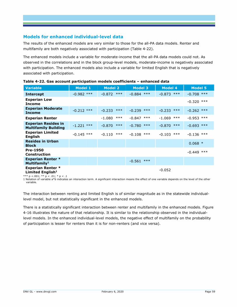
DNV GL – www.dnvgl.com February 6, 2020 Page 59
Models for enhanced individual-level data
The results of the enhanced models are very similar to those for the all-PA data models. Renter and
multifamily are both negatively associated with participation (Table 4-22).
The enhanced models include a variable for moderate-income that the all-PA data models could not. As
observed in the correlations and in the block group-level models, moderate-income is negatively associated
with participation. The enhanced models also include a variable for limited English that is negatively
associated with participation.
Table 4-22. Gas account participation models coefficients – enhanced data
Variable Model 1 Model 2 Model 3 Model 4 Model 5
Intercept -0.982 *** -0.872 *** -0.884 *** -0.873 *** -0.708 ***
Experian Low
Income -0.320 ***
Experian Moderate Income
-0.212 *** -0.233 *** -0.239 *** -0.233 *** -0.262 ***
Experian Renter -1.080 *** -0.847 *** -1.069 *** -0.953 ***
Experian Resides in Multifamily Building
-1.221 *** -0.870 *** -0.780 *** -0.870 *** -0.693 ***
Experian Limited English
-0.145 *** -0.110 *** -0.108 *** -0.103 *** -0.136 ***
Resides in Urban
Block 0.068 *
Pre-1950 Construction
-0.449 ***
Experian Renter * Multifamily1
-0.561 ***
Experian Renter * Limited English1
-0.052
*** p <.001; ** p < .01; * p < .1
1 Notation of variable a*b indicates an interaction term. A significant interaction means the effect of one variable depends on the level of the other variable.
The interaction between renting and limited English is of similar magnitude as in the statewide individual-
level model, but not statistically significant in the enhanced models.
There is a statistically significant interaction between renter and multifamily in the enhanced models. Figure
4-16 illustrates the nature of that relationship. It is similar to the relationship observed in the individual-
level models. In the enhanced individual-level models, the negative effect of multifamily on the probability
of participation is lesser for renters than it is for non-renters (and vice versa).
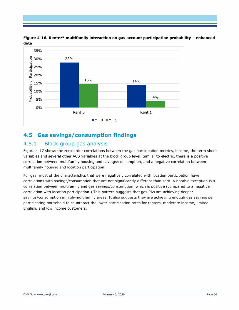
DNV GL – www.dnvgl.com February 6, 2020 Page 60
Figure 4-16. Renter* multifamily interaction on gas account participation probability – enhanced
data
4.5 Gas savings/consumption findings
4.5.1 Block group gas analysis
Figure 4-17 shows the zero-order correlations between the gas participation metrics, income, the term sheet
variables and several other ACS variables at the block group level. Similar to electric, there is a positive
correlation between multifamily housing and savings/consumption, and a negative correlation between
multifamily housing and location participation.
For gas, most of the characteristics that were negatively correlated with location participation have
correlations with savings/consumption that are not significantly different than zero. A notable exception is a
correlation between multifamily and gas savings/consumption, which is positive (compared to a negative
correlation with location participation.) This pattern suggests that gas PAs are achieving deeper
savings/consumption in high-multifamily areas. It also suggests they are achieving enough gas savings per
participating household to counteract the lower participation rates for renters, moderate income, limited
English, and low income customers.
28%
14%15%
4%
0%
5%
10%
15%
20%
25%
30%
35%
Rent 0 Rent 1
Pro
bability o
f Part
icip
ation
MF 0 MF 1
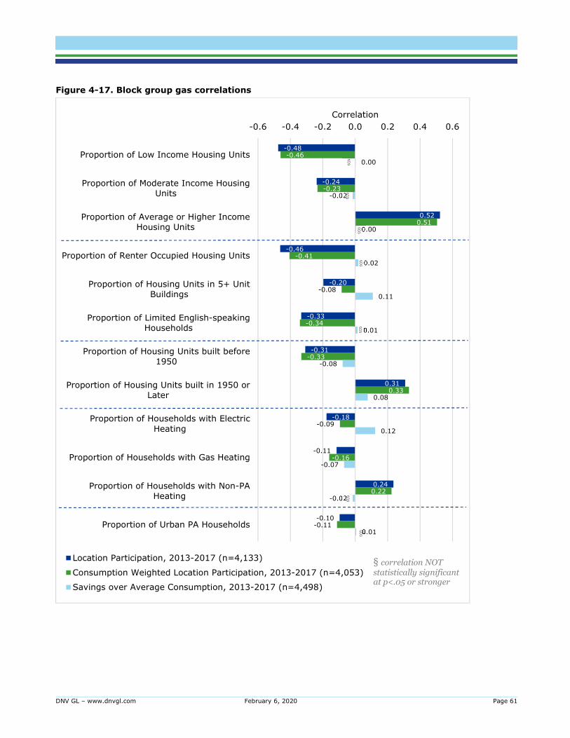
DNV GL – www.dnvgl.com February 6, 2020 Page 61
Figure 4-17. Block group gas correlations
-0.48
-0.24
0.52
-0.46
-0.20
-0.33
-0.31
0.31
-0.18
-0.11
0.24
-0.10
-0.46
-0.23
0.51
-0.41
-0.08
-0.34
-0.33
0.33
-0.09
-0.16
0.22
-0.11
0.00
-0.02
0.00
0.02
0.11
0.01
-0.08
0.08
0.12
-0.07
-0.02
0.01
-0.6 -0.4 -0.2 0.0 0.2 0.4 0.6
Proportion of Low Income Housing Units
Proportion of Moderate Income HousingUnits
Proportion of Average or Higher IncomeHousing Units
Proportion of Renter Occupied Housing Units
Proportion of Housing Units in 5+ UnitBuildings
Proportion of Limited English-speakingHouseholds
Proportion of Housing Units built before1950
Proportion of Housing Units built in 1950 orLater
Proportion of Households with Electric
Heating
Proportion of Households with Gas Heating
Proportion of Households with Non-PAHeating
Proportion of Urban PA Households
Correlation
Location Participation, 2013-2017 (n=4,133)
Consumption Weighted Location Participation, 2013-2017 (n=4,053)
Savings over Average Consumption, 2013-2017 (n=4,498)
§ correlation NOT statistically significant at p<.05 or stronger

DNV GL – www.dnvgl.com February 6, 2020 Page 62
Ordinary least squares (OLS) models revealed interesting dynamics between low and moderate income,
renter, multifamily, and limited English regarding savings/consumption. When low income, moderate
income, renter, multifamily, and limited English are in the model (model 1 in Table 4-23), moderate income,
renter, and limited English all become statistically significant predictors of savings/consumption. The
strength of the effect of multifamily (relative to the zero-order correlation) is reduced in model 1 while the
effect of moderate income is increased. This suggests that the covariation between moderate income and
multifamily status reduces the overall effect (correlation) of moderate income. When that effect is controlled
for in the model, moderate income becomes a significant predictor. The interaction between multifamily and
renter (model 4) helps explain why the renter effects in the models are stronger than the correlations.
Table 4-23. Gas savings/consumption model results
Variable Model 1 Model 2 Model 3 Model 4
Coefficient Coefficient Coefficient Coefficient
Intercept 0.057 *** 0.056 *** 0.061 *** 0.059 ***
Proportion of Households at less than 56% of Statewide Median Income
-0.003 0.000 -0.027 *** -0.005
Proportion of Households at 56 - 85% of Statewide Median Income
-0.044 *** -0.043 *** -0.036 *** -0.041 ***
Proportion of Renter Occupied Housing Units
-0.036 *** -0.031 *** -0.030 *** -0.039 ***
Proportion of Housing Units in 5+ Unit Buildings
0.046 *** 0.045 *** 0.013 * 0.022 *
Proportion of Limited English-speaking Households
0.030 ** 0.020 * 0.027 **
Proportion of Households at less than 56% of Statewide Median Income * Proportion of Housing Units in 5+ Unit Buildings
0.082 ***
Proportion of Renter Occupied Housing Units * Proportion of Housing Units in 5+ Unit Buildings
0.037 **
* Statistically significantly different from 0 at p<.05 or stronger
There are several significant interactions occurring in the gas models. First, as shown in Model 3 above,
multifamily and low income interact. The effect of multifamily inverts the low income effect such that at high
levels of low income and multifamily, we expect higher participation rates, but at high levels of low income
and low levels of multifamily, we expect very low participation rates (as measured by savings/consumption;
Figure 4-18). This is the same pattern observed in the electric analysis. Even though the main effect (zero-
order correlation) of low income is lowered participation rates, the significant interaction supports the
hypothesis that multifamily programs, particularly low income multifamily programs, are achieving relatively
deep savings.

DNV GL – www.dnvgl.com February 6, 2020 Page 63
Figure 4-18. Interaction of low income and multifamily on gas savings/consumption
As shown in Model 4 above, there is also a significant interaction between multifamily and renting. Renting
has a stronger effect on non-multifamily buildings than in multifamily buildings, as indicated by the distance
between the lines at MF=0% and MF=100% in Figure 4-19. In multifamily buildings, there is almost no
distinction in expected savings/consumption ratios based on renting status. However, in non-multifamily
buildings, renters can be expected to have lower savings/consumption ratios than non-renters.
Figure 4-19. Interaction of rent and multifamily on gas savings/consumption
4.5.2 Individual-level gas analysis – Statewide
Figure 4-20 shows the statewide, zero-order, account-level correlations between the gas participation
metrics, multifamily, renter, urban, and pre-1950 construction (other characteristics are not available at the
account level). Account participation correlations are repeated here for the sake of contrast. Unlike the
0%
2%
4%
6%
8%
10%
12%
Low Income 0% Low Income 50% Low Income 100%
Expecte
d P
art
icip
ation R
ate
s
MF 0% MF 50% MF 100%
0%
1%
2%
3%
4%
5%
6%
7%
8%
9%
MF 0% MF 50% MF 100%
Expecte
d P
art
icip
ation R
ate
s
Rent 0% Rent 50% Rent 100%

DNV GL – www.dnvgl.com February 6, 2020 Page 64
block-group level correlations, the account-level correlations with savings/consumption go in the same
direction as for account participation.
Figure 4-20. Individual-level correlations with savings over consumption, statewide gas
Table 4-24 shows results for models that DNV GL used to isolate the effects of the different variables
independently of the other variables. In all three models, the coefficients go in the same direction and are
approximately the same magnitude as the zero-order correlations. This means that the covariation between
the various characteristics (e.g., multifamily residents tend to rent) does not mask or substantially change
the effects of any singular characteristic.
Table 4-24. Individual-level savings over consumption models, statewide gas
Variable Model 1 Model 2 Model 3
Intercept 0.028 *** 0.028 *** 0.032 ***
Renter -0.009 *** -0.009 *** -0.006 ***
Resides in multifamily
building -0.015 *** -0.017 *** -0.015 ***
Renter * Multifamily 1 0.002 0.000
Resides in Urban block 0.001
Pre-1950 construction -0.009 ***
*** p <.001; ** p < .01; * p < .1
1 Notation of variable a*b indicates an interaction term. A significant interaction means the effect of one variable depends on the level of the other
variable.
4.5.3 Individual-level gas analysis – Enhanced
Figure 4-21 shows the Eversource-only, enhanced data, zero-order account-level correlations between the
electric participation metrics, income, renter, multifamily, limited English, construction vintage, and urban.
-0.09
-0.13
-0.02
-0.09
-0.06
-0.07
-0.01
-0.07
-0.15 -0.10 -0.05 0.00 0.05 0.10 0.15
Multifamily
Renter
Urban
Pre-1950 Construction
Correlation
Account Participation, 2013-2017
Savings/ Avg. Consumption, 2013-2017all correlations statistically significant p<.01

DNV GL – www.dnvgl.com February 6, 2020 Page 65
Account participation correlations are repeated here for the sake of contrast. Unlike the block-group level
correlations and similar to the statewide account-level correlations, the enhanced account-level correlations
with savings/consumption go in the same direction as for enhanced account participation.
Figure 4-21. Individual-level correlations with savings over consumption, enhanced gas
Table 4-25 shows results for models that DNV GL used to isolate the effects of the different variables
independently of the other variables. Except for low and renter, the coefficients for each of the variables are
similar to the zero-order correlations. This means the overall effect of the variable (correlation) is similar to
the independent effect when controlling for the covariation with the other characteristics (coefficients).
The strength of the effects for low income and renter was reduced in the models relative to their
correlations. This suggests that some of the overall effect (correlation) of these variables is because of their
overlap with other variables in the model. For example, renter and multifamily are correlated, so the overall
negative effect of renters is partially due to the overlapping negative effect of multifamily.
-0.09
-0.04
0.11
-0.18
-0.20
-0.04
-0.09
-0.02
-0.05
-0.02
0.06
-0.12
-0.12
-0.03
-0.07
-0.01
-0.30 -0.20 -0.10 0.00 0.10 0.20 0.30
Low Income
Moderate Income
Average or Higher Income
Renter
Multifamily
Limited English
Pre-1950 Construction
Urban
Correlation
Account Participation, 2013-2017
Savings/ Avg. Consumption, 2013-2017
all correlations statistically significant p<.01
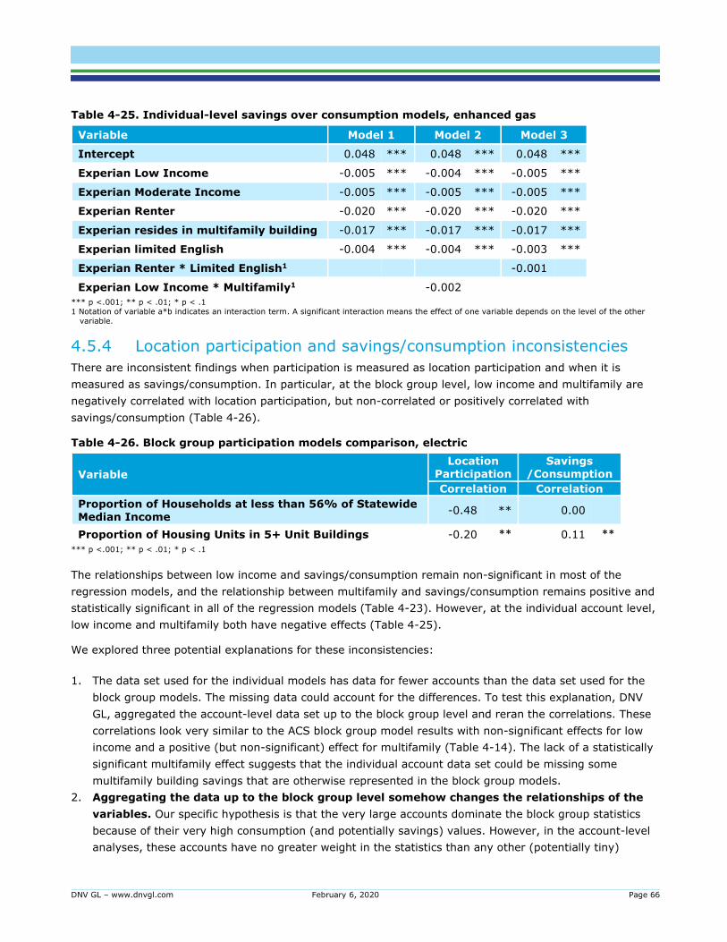
DNV GL – www.dnvgl.com February 6, 2020 Page 66
Table 4-25. Individual-level savings over consumption models, enhanced gas
Variable Model 1 Model 2 Model 3
Intercept 0.048 *** 0.048 *** 0.048 ***
Experian Low Income -0.005 *** -0.004 *** -0.005 ***
Experian Moderate Income -0.005 *** -0.005 *** -0.005 ***
Experian Renter -0.020 *** -0.020 *** -0.020 ***
Experian resides in multifamily building -0.017 *** -0.017 *** -0.017 ***
Experian limited English -0.004 *** -0.004 *** -0.003 ***
Experian Renter * Limited English1 -0.001
Experian Low Income * Multifamily1 -0.002
*** p <.001; ** p < .01; * p < .1
1 Notation of variable a*b indicates an interaction term. A significant interaction means the effect of one variable depends on the level of the other
variable.
4.5.4 Location participation and savings/consumption inconsistencies
There are inconsistent findings when participation is measured as location participation and when it is
measured as savings/consumption. In particular, at the block group level, low income and multifamily are
negatively correlated with location participation, but non-correlated or positively correlated with
savings/consumption (Table 4-26).
Table 4-26. Block group participation models comparison, electric
Variable
Location Participation
Savings /Consumption
Correlation Correlation
Proportion of Households at less than 56% of Statewide Median Income
-0.48 ** 0.00
Proportion of Housing Units in 5+ Unit Buildings -0.20 ** 0.11 ** *** p <.001; ** p < .01; * p < .1
The relationships between low income and savings/consumption remain non-significant in most of the
regression models, and the relationship between multifamily and savings/consumption remains positive and
statistically significant in all of the regression models (Table 4-23). However, at the individual account level,
low income and multifamily both have negative effects (Table 4-25).
We explored three potential explanations for these inconsistencies:
1. The data set used for the individual models has data for fewer accounts than the data set used for the
block group models. The missing data could account for the differences. To test this explanation, DNV
GL, aggregated the account-level data set up to the block group level and reran the correlations. These
correlations look very similar to the ACS block group model results with non-significant effects for low
income and a positive (but non-significant) effect for multifamily (Table 4-14). The lack of a statistically
significant multifamily effect suggests that the individual account data set could be missing some
multifamily building savings that are otherwise represented in the block group models.
2. Aggregating the data up to the block group level somehow changes the relationships of the
variables. Our specific hypothesis is that the very large accounts dominate the block group statistics
because of their very high consumption (and potentially savings) values. However, in the account-level
analyses, these accounts have no greater weight in the statistics than any other (potentially tiny)
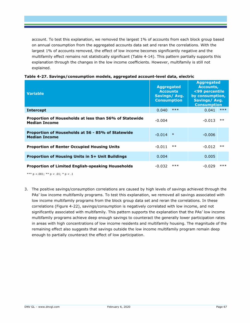
DNV GL – www.dnvgl.com February 6, 2020 Page 67
account. To test this explanation, we removed the largest 1% of accounts from each block group based
on annual consumption from the aggregated accounts data set and reran the correlations. With the
largest 1% of accounts removed, the effect of low income becomes significantly negative and the
multifamily effect remains not statistically significant (Table 4-14). This pattern partially supports this
explanation through the changes in the low income coefficients. However, multifamily is still not
explained.
Table 4-27. Savings/consumption models, aggregated account-level data, electric
Variable
Aggregated
Accounts Savings/ Avg. Consumption
Aggregated Accounts,
<99 percentile by consumption,
Savings/ Avg. Consumption
Intercept 0.040 *** 0.041 ***
Proportion of Households at less than 56% of Statewide Median Income
-0.004 -0.013 **
Proportion of Households at 56 - 85% of Statewide Median Income
-0.014 * -0.006
Proportion of Renter Occupied Housing Units -0.011 ** -0.012 **
Proportion of Housing Units in 5+ Unit Buildings 0.004 0.005
Proportion of Limited English-speaking Households -0.032 *** -0.029 ***
*** p <.001; ** p < .01; * p < .1
3. The positive savings/consumption correlations are caused by high levels of savings achieved through the
PAs’ low income multifamily programs. To test this explanation, we removed all savings associated with
low income multifamily programs from the block group data set and reran the correlations. In these
correlations (Figure 4-22), savings/consumption is negatively correlated with low income, and not
significantly associated with multifamily. This pattern supports the explanation that the PAs’ low income
multifamily programs achieve deep enough savings to counteract the generally lower participation rates
in areas with high concentrations of low income residents and multifamily housing. The magnitude of the
remaining effect also suggests that savings outside the low income multifamily program remain deep
enough to partially counteract the effect of low participation.

DNV GL – www.dnvgl.com February 6, 2020 Page 68
Figure 4-22. Block group correlations, gas, no LIMF savings
-0.50
-0.23
0.55
-0.48
-0.22
-0.36
-0.31
0.31
-0.20
-0.11
0.25
-0.10
-0.46
-0.23
0.50
-0.40
-0.07
-0.34
-0.33
0.33
-0.09
-0.16
0.22
-0.11
-0.10
0.00
0.09
-0.08
0.01
-0.07
-0.11
0.11
0.04
-0.05
0.03
-0.01
-0.6 -0.4 -0.2 0.0 0.2 0.4 0.6
Proportion of Low Income Housing Units
Proportion of Moderate Income Housing Units
Proportion of Average or Higher Income Housing Units
Proportion of Renter Occupied Housing Units
Proportion of Housing Units in 5+ Unit Buildings
Proportion of Limited English-speaking Households
Proportion of Housing Units built before 1950
Proportion of Housing Units built in 1950 or Later
Proportion of Households with Electric Heating
Proportion of Households with Gas Heating
Proportion of Households with Non-PA Heating
Proportion of Urban PA Households
Correlation
Location Participation, 2013-2017 (n=4,126)
Consumption Weighted Location Participation, 2013-2017 (n=4,055)
Savings over Average Consumption, 2013-2017 (n=4,521)
§ correlation NOT
statistically significant at
p<.05 or stronger

DNV GL – www.dnvgl.com February 6, 2020 Page 69
5 CONCLUSIONS, RECOMMENDATIONS, AND CONSIDERATIONS
5.1 Conclusions
5.1.1 Location participation rates for 2013-2017 are negatively associated with all three term sheet variables: moderate-income
households, renter households, and limited English-speaking
households.
These relationships hold across the block group-level correlations and models as well as the individual-level
correlations and models. This indicates that populations represented by the term sheet participate at lower
levels than other populations.
5.1.2 PA efforts to obtain participation from large multifamily locations
have resulted in some inclusion of the populations outlined in the
term sheet.
There is evidence that the PAs have had some success in getting multifamily locations to participate,
especially when savings/consumption is considered. Because multifamily is correlated with renters, low-
income, and limited English speaking, the PAs’ success with multifamily locations has enabled some of the
term sheet-related populations to obtain benefits from the programs.
5.1.3 When participation is measured using 2013-2017
savings/consumption, it is positively correlated with low income and multifamily at the block group level.
In contrast to location participation rates, participation measured as the ratio of savings to consumption is
positively correlated with: low income, renter, multifamily, and limited English. However, these positive
correlations hold only at the block group level of analysis. In the individual-level analyses, the low income
and the term sheet variables are still negatively associated with participation measured as
savings/consumption. We suspect but have not been able to fully confirm that the differences between the
block group-level and individual-level findings are caused by the participation of the largest MF buildings.
The very large MF buildings tend to dominate the block group totals and averages. However, those buildings
have greater weight than any other account in the individual-level analyses. The inconsistency between the
block group and individual level models for this metric of participation indicates that the risk of ecological
fallacy is greater in these analyses than in the location participation analyses.
5.1.4 Location participation rates for 2013-2017 are affected by multiple factors.
Location participation is negatively correlated with: low income, pre-1950 construction, and PA-delivered
heating fuel (electric or gas). Location participation is positively correlated with average or higher income,
post-1950 construction, and receiving heating fuel from a non-PA source.
5.1.5 Most of the variables investigated are correlated with each other,
especially in the ACS data.
This suggests that increasing participation among one of the term sheet-related populations will also
increase participation among the other term sheet-related populations. For example, increasing participation

DNV GL – www.dnvgl.com February 6, 2020 Page 70
among renters will also create some increased participation among limited English speakers (and vice
versa).
5.1.6 Term sheet-related populations are geographically clustered in
urban areas.
In addition to being correlated with each other, the term sheet variables also exhibit spatial clustering in
urban areas. This suggests that the PAs’ community outreach partnerships and continued engagement with
local community stakeholders including the action agencies and civic groups are likely to have a positive
impact on the term sheet populations and benefit from positive word of mouth from trusted voices at the
local level.
5.1.7 Limited-English speakers are more likely to rent, and renters are
less likely to participate.
The tendency to rent explains some but not all of the reduced participation rates of the limited-English
population. Program designs that increase the participation of renters will also increase participation of
limited-English speakers as a “bonus.” However, additional outreach or program design would be required to
fully address the population of limited-English speakers.
5.1.8 The effects of the examined variables on participation are similar
in both electric and gas markets.
This indicates that the participation barriers faced by the populations identified by the term sheet variables
are probably similar for both electric and gas participation.
5.1.9 The individual-level models are mostly consistent with the block group-level models.
This indicates that conclusions based on the block group-level information are unlikely to suffer from
ecological fallacy for the analyses examined in this study. However, one should always be wary of the
possibility of ecological fallacy in the future. In particular, the effects of multifamily tended to be inconsistent
between the block group level and individual level models.
5.1.10 Comparison to the Market Barriers Study
The Market Barriers Study conducted primary research (including over 1,700 surveys and in-depth
interviews) to explore nonparticipant characteristics, investigate participation barriers, and identify PA
engagement opportunities. Key findings from that study, and their relationship to this study’s findings, are
shown in Table 1-1. Findings from both studies were generally consistent, and there were no cases of
completely contradictory findings.

DNV GL – www.dnvgl.com February 6, 2020 Page 71
Table 5-1. Key findings of residential nonparticipant studies
Residential Nonparticipant
Market Barriers
Residential
Nonparticipant
Customer Profile
Discussion
Self-reported program participation agreed 68% with participation
as determined by tracking data.
This is a high level of agreement
between self-reported participation
and the tracking data. In addition,
most (88%) of the self-reported
participants that were not identified
via the tracking data indicated their
participation took place outside the
5-year window of tracking data.
Participants identified via the
tracking data but not self-reporting
tended to be renters, live in
multifamily buildings, and/or live in
their current home for 4 or fewer
years.
Nonparticipants were more likely
to live in:
• Rental units
• Low to moderate income
households
• Households that speak a non-
English language or report
having limited English
proficiency
Renters, customers who live
in moderate income
households, and customers
living in limited-English
speaking households are less
likely to participate than
customers without these
characteristics.
The findings are consistent across
both studies.

DNV GL – www.dnvgl.com February 6, 2020 Page 72
Residential Nonparticipant
Market Barriers
Residential
Nonparticipant
Customer Profile
Discussion
Nonparticipants also tend to:
• Have lower education levels
• Be less aware of Mass Save
• Do not fully trust government,
landlords, or free offers
• Prioritize time and resources
for other issues such as food
and well-being
• Need additional information or
understanding of Mass Save
offerings, processes, and
benefits
• Perceive energy efficiency as
irrelevant or not applicable to
them
No related findings
These findings highlight some of the
increased depth and additional topics
the Market Barriers study was able
to address beyond the data that
were available to the Nonparticipant
Customer Profile study.
Nonparticipant renters are more
likely to:
• Reside in lowest participating
Census tracts
• Self-identify as low income
Most of the variables
investigated are correlated
with each other, especially in
the ACS block group data.
Term sheet-related
populations are
geographically clustered in
urban areas.
The findings are consistent across
both studies.
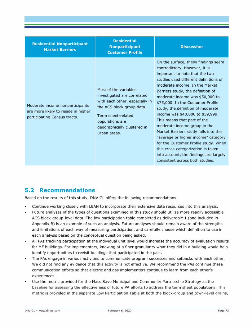
DNV GL – www.dnvgl.com February 6, 2020 Page 73
Residential Nonparticipant
Market Barriers
Residential
Nonparticipant
Customer Profile
Discussion
Moderate income nonparticipants
are more likely to reside in higher
participating Census tracts.
Most of the variables
investigated are correlated
with each other, especially in
the ACS block group data.
Term sheet-related
populations are
geographically clustered in
urban areas.
On the surface, these findings seem
contradictory. However, it is
important to note that the two
studies used different definitions of
moderate income. In the Market
Barriers study, the definition of
moderate income was $50,000 to
$75,000. In the Customer Profile
study, the definition of moderate
income was $40,000 to $59,999.
This means that part of the
moderate income group in the
Market Barriers study falls into the
“average or higher income” category
for the Customer Profile study. When
this cross-categorization is taken
into account, the findings are largely
consistent across both studies.
5.2 Recommendations
Based on the results of this study, DNV GL offers the following recommendations:
• Continue working closely with LEAN to incorporate their extensive data resources into this analysis.
• Future analyses of the types of questions examined in this study should utilize more readily accessible
ACS block-group-level data. The low participation table completed as deliverable 1 (and included in
Appendix B) is an example of such an analysis. Future analyses should remain aware of the strengths
and limitations of each way of measuring participation, and carefully choose which definition to use in
each analysis based on the conceptual question being asked.
• All PAs tracking participation at the individual unit level would increase the accuracy of evaluation results
for MF buildings. For implementers, knowing at a finer granularity what they did in a building would help
identify opportunities to revisit buildings that participated in the past.
• The PAs engage in various activities to communicate program successes and setbacks with each other.
We did not find any evidence that this activity is not effective. We recommend the PAs continue these
communication efforts so that electric and gas implementers continue to learn from each other’s
experiences.
• Use the metric provided for the Mass Save Municipal and Community Partnership Strategy as the
baseline for assessing the effectiveness of future PA efforts to address the term sheet populations. This
metric is provided in the separate Low Participation Table at both the block-group and town-level grains,

DNV GL – www.dnvgl.com February 6, 2020 Page 74
and is included in this report in Appendix B. In general, we recommend examining multiyear trends
rather than focusing on singular years.
5.3 Considerations
DNV GL also offers the following considerations:
• Future analyses should continue to assess and leverage data like Tax Assessor data to refine models.
For example, home type (e.g. Cape Cod, Victorian, Ranch) and construction date can help indicate
potential barriers. Home value might also be usable as a proxy for income.
• Given the overlap and geographic clustering of term sheet variables, the PAs may benefit from
examining their time series billing and tracking data to identify individuals who both participated in the
programs, and are in areas of high interest. Alternatively or in addition, PAs could use these geographic
clusters to inform future implementation of the Municipal and Community Partnership Strategy.
• Continue to explore program designs that will help these populations overcome the participation barriers
that they face. From our work nationally, DNV GL recognizes that these types of questions and
populations are not a unique consideration to MA PAs. The PAs should consider a meta-review of how
their ACEEE ranked nationally leading programs both set the stage for other states, as well as where
there are opportunities to quickly assimilate new program designs and ideas identified in the literature
review.
• Use the bivariate maps provided in this study and other methods of identifying geospatial areas to target
program outreach efforts. The bivariate maps provide a way to identify the block groups that are the
greatest outliers in terms of the high incidence of term sheet variables and low participation rates.
• Continue to explore program designs to increase renter participation. Also, continue to explore program
designs that specifically address limited-English speakers above and beyond the renter programs.
• The present study found evidence that there are significant interactions between multifamily buildings
and the term sheet variables that affect participation rates. The PAs treat multifamily locations
differently than single-family locations, and in some cases even record billing data differently. The
current study was not able to fully explore or explain all of these relationships due to budget and
schedule constraints. Carefully examine whether the recently completed Navigant MF Census study can
shed additional light on unanswered questions resulting from this study. If important questions remain,
consider conducting a follow-up multifamily study that attempts to fill in those gaps. A specific question
that should be considered in the scope of such a follow-up study is whether MF locations should use a
different participation metric than SF locations, or if using the same metric, whether it should be
considered separately for MF and SF locations.
• For the findings related to non-term sheet variables (construction year, urban/rural, and non-PA heating
fuel), limitations such as the skew in the distribution of urban versus rural block groups and the handling
of data related to delivered fuel projects should be considered more closely before taking action on
these findings.

DNV GL – www.dnvgl.com February 6, 2020 Page 75
6 APPENDIX A: PARTICIPANT/NONPARTICIPANT LIST PREPARATION
This appendix contains additional details of how we prepared the PNP list. These steps were previously
documented in a memo delivered to the working group on May 17, 2019.
Tracking data preparation
After combining the 2013 through 2017 residential tracking data, we had a total of 7,569,297 records across
all PAs, fuels, and year. These represent 1,087,153 unique account ids. Approximately 25% of the records
have a missing account id and are associated with the residential lighting program or residential products
program. Another 25% of the records are associated with account ids that appear at least 11 times per
year.
The following table shows how the number of unique accounts is distributed among fuels, PAs, and years.
These counts are all within 8% (most within 5%) of previous counts provided by DNV GL. The discrepancies
are caused by continuous updating of the databases since the previous counts were provided based on
ongoing clarification from the PAs.
Table 6-1. Unique accounts in tracking data (Fuel*PA*year)
Fuel PA 2013 2014 2015 2016 2017 Unique
Accounts
2013-2017
E Cape Light Compact
10,165 13,580 13,725 11,462 14,722 50,290
E Eversource 63,526 80,956 78,387 74,094 73,615 305,285
E National Grid 96,893 81,549 70,199 67,785 73,071 362,700
E Unitil 497 741 1,096 1,427 1,463 4,556
Electric Total 173,094 178,840 165,422 156,784 164,888 722,831
G Berkshire 2,073 2,132 1,773 1,529 1,762 8,064
G Columbia 12,668 12,291 13,472 16,726 16,030 66,962
G Eversource 14,545 12,602 14,262 14,331 18,326 62,203
G Liberty 1,194 1,669 1,545 1,554 1,625 7,146
G National Grid 55,333 50,996 48,330 36,752 43,611 218,501
G Unitil 127 282 330 458 367 1,446
Gas Total 85,940 79,972 79,712 71,350 81,721 364,322
Grand Total 259,034 258,812 245,134 228,134 246,609 1,087,153
Billing data preparation
The residential and C&I billing data were prepared separately but in similar ways.
Residential
The billing data processing started with the merged 2017 residential billing data from all of the PAs. The
grain of these data is multiple records per account id by month. We started with 52,925,322 records across
the state.

DNV GL – www.dnvgl.com February 6, 2020 Page 76
Step 1: Deduplicate down to unique accounts by month. Some accounts have multiple lines per
month, such as when they receive a bill correction. This step reduced the list down to a single record per
month per account. The final record count statewide was 47,511,738.
Step 2: Deduplicate down to unique accounts. In the output from step 1, we would see 12 records per
account that were active the entire year. This step reduces the data down to a single record per account
that was active sometime in 2017. We ended with 4,256,178 records after this step, for a reduction of
approximately 90%. Reducing the count by a factor of approximately 10 makes sense because some
accounts would not be active the entire year or receive bills every month. Each PA saw similar levels of
reduction. These counts are generally within 1% or less of the counts in the summary of data completeness
from the 2017 data intake process. The one exception is Columbia, for which we have approximately 13,000
additional unique account ids. All of the Columbia records appear to be legitimate locations.
Table 6-2. Residential unique accounts by fuel and PA
Fuel PA Input
Residential Billing Data
Step 1: Accounts *
Month
Step 2: Unique
Accounts
E Cape Light Compact
3,917,354 2,101,570 191,267
E Eversource 16,139,224 12,619,015 1,248,640
E National Grid 13,962,591 13,950,887 1,170,963
E Unitil 288,309 285,792 29,140
Electric Total 34,307,478 28,957,264 2,640,010
G Berkshire 415,850 415,418 35,310
G Columbia 4,386,899 4,362,685 349,432
G Eversource 3,217,134 3,179,842 316,173
G Liberty 572,665 572,441 51,917
G National Grid 9,865,803 9,865,799 846,678
G Unitil 159,493 158,289 16,658
Gas Total 18,617,844 18,554,474 1,616,168
Grand Total 52,925,322 47,511,738 4,256,178
C&I
The processing of the C&I data followed the same first two steps as residential. We then added an additional
filter to remove C&I records that were not residential. The billing data processing started with the merged
2017 C&I billing data from all of the PAs. The grain of these data is approximately account id by month. We
started with 6,315,653 records across the state.
Step 1: Deduplicate down to unique accounts by month. Some accounts have multiple lines per
month, such as when they receive a bill correction. This step reduced the list down to a single record per
month per account. The final statewide record count was 6,204, 575.
Step 2: Deduplicate down to unique accounts. In the output from step 1, we would see 12 records per
account that were active the entire year. This step reduces the data down to a single record per account

DNV GL – www.dnvgl.com February 6, 2020 Page 77
that was active sometime in 2017. We ended with 538,598 records after this step, for a reduction of
approximately 90%. Reducing the count by a factor of approximately 10 makes sense because some
accounts would not be active the entire year or receive bills every month. Each PA saw similar levels of
reduction. These counts are within 1% of the 2017 summary of data completeness. Columbia was an
exception here as well, with an additional 1,500 records on our list. Again, those all appear to be legitimate
locations.
Table 6-3. C&I Unique accounts by fuel and PA (before removing nonresidential)
Fuel PA Input
Residential Billing Data
Step 1: Accounts *
Month
Step 2: Unique
Accounts
E Cape Light
Compact 283,947 279,234 25,535
E Eversource 2,017,772 1,925,861 171,420
E National Grid 2,124,855 2,123,052 181,765
E Unitil 42,479 40,694 3,909
Electric Total 4,469,053 4,368,841 382,629
G Berkshire 63,632 63,566 5,380
G Columbia 468,886 468,505 35,502
G Eversource 339,869 329,636 30,187
G Liberty 48,757 48,668 4,334
G National Grid 907,108 907,107 78,730
G Unitil 18,348 18,252 1,836
Gas Total 1,846,600 1,835,734 155,969
Grand Total 6,315,653 6,204,575 538,598
Final billing file
The final step for preparing the billing file was to merge the residential and C&I data sets and then remove
records that do not appear to be residential.
Remove nonresidential records. The final step was to remove records that could not be identified as
single-family or multi-family through the tax assessor data and any that were clearly streetlights, cell phone
boosters, and wells. We also checked account names for variations on “housing authority” to make sure we
included as many of these records as we could. We applied the following filters during this step (see
Appendix A for documentation of how we classified each rate code):
4. Remove records according to rate codes. This resulted in a reduction of 37,319 records.
5. Remove records that were coded as neither residential nor multifamily based on tax assessor use codes.
This resulted in a reduction of 413,477 records.
6. Remove records with the following text strings in the customer name. This resulted in a reduction of
2,727 records.
'VERIZON' 'CINGULAR' 'T-MOBILE'
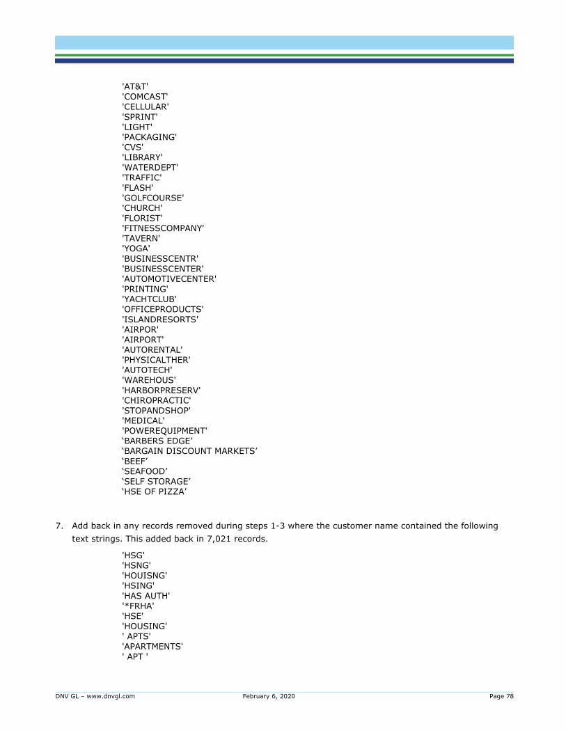
DNV GL – www.dnvgl.com February 6, 2020 Page 78
'AT&T' 'COMCAST' 'CELLULAR'
'SPRINT' 'LIGHT' 'PACKAGING' 'CVS' 'LIBRARY' 'WATERDEPT' 'TRAFFIC'
'FLASH' 'GOLFCOURSE' 'CHURCH' 'FLORIST' 'FITNESSCOMPANY' 'TAVERN' 'YOGA'
'BUSINESSCENTR' 'BUSINESSCENTER' 'AUTOMOTIVECENTER' 'PRINTING' 'YACHTCLUB' 'OFFICEPRODUCTS'
'ISLANDRESORTS' 'AIRPOR' 'AIRPORT' 'AUTORENTAL' 'PHYSICALTHER' 'AUTOTECH' 'WAREHOUS'
'HARBORPRESERV' 'CHIROPRACTIC' 'STOPANDSHOP' 'MEDICAL' 'POWEREQUIPMENT' ‘BARBERS EDGE’ ‘BARGAIN DISCOUNT MARKETS’
‘BEEF’ ‘SEAFOOD’ ‘SELF STORAGE’ ‘HSE OF PIZZA’
7. Add back in any records removed during steps 1-3 where the customer name contained the following
text strings. This added back in 7,021 records.
'HSG' 'HSNG' 'HOUISNG' 'HSING'
'HAS AUTH' '*FRHA' 'HSE' 'HOUSING' ' APTS' 'APARTMENTS'
' APT '

DNV GL – www.dnvgl.com February 6, 2020 Page 79
The final record counts by fuel and PA follow.
Table 6-4. Final record counts by fuel and PA
Fuel PA From Residential
Billing From C&I Billing Total
E Cape Light Compact 190,212 1,703 191,915
E Eversource 1,245,185 34,552 1,279,737
E National Grid 1,168,581 38,961 1,207,542
E Unitil 29,103 354 29,457
Total Electric 2,633,081 75,570 2,708,651
G Berkshire 35,223 621 35,844
G Columbia 348,951 3,262 352,213
G Eversource 315,619 3,375 318,994
G Liberty 51,867 147 52,014
G National Grid 845,449 8,989 854,438
G Unitil 16,641 134 16,775
Total Gas 1,613,750 16,528 1,630,278
Grand Total 4,246,831 92,098 4,338,929
Set participation flags
Account participation
We determined account participation by identifying any account ids in the final billing file that also appeared
in the final tracking file.
Address participation
We determined to address participation by identifying any addresses in the final billing file that also
appeared in the final tracking file. Addresses were matched based on the combination of Address1 (street
number and name), Address2 (supplemental address information), standardized city name, and zip code.
Because these were matches made on text strings, literal differences such as spelling out “street” versus
abbreviating it as “st” would fail to match.
Location participation
Most of the records (98% of residential, 90% of C&I) had a point-level geocoded latitude and longitude
location. For those records, if any records at a particular latitude*longitude had either account participation
or address participation, then location participation was set to 1. For records that lacked point-level
geocoded locations, location-level participation is undefined (coded as -99).

DNV GL – www.dnvgl.com February 6, 2020 Page 80
We also performed a second match directly between geocoded locations in the 2013-2017 tracking data and
the 2017 billing data to identify locations where participation occurred but the current account id was not in
the 2017 billing data and the address text strings did not match.
Other variables
ID low-income participants
Low-income participants were identified based on a crosswalk of specific rate codes previously provided by
the PAs. The following rate codes by PA were identified as low income. See Appendix A for documentation of
how we classified each rate code.
Add current account holder
The PAs provided current account holder lists in mid-2018. We flagged any account id in these lists as a
current account holder.
Experian variables
Below are relevant excerpts from the Experian data dictionary that provide additional details about how
Experian created some of the data fields that DNV GL used.
0113A - Combined Homeowner – DNV GL used Combined Homeowner as one of our checks of our Renter
flag. We coded R and T as renters and H as owners. Other values were coded as neither.
Combined homeowner is a mixture of several data elements / fields. This element provides these separate
data components in a single position. Homeowner information indicates the likelihood of a consumer owning
a home, and is received from tax assessor and deed information. For records where exact Homeownership
information is not available, homeownership propensity is calculated using a proprietary statistical model
which predicts the likelihood of homeownership. Renter status is derived from self reported data. Unit
numbers are not used to infer rented status because units may be owner condominium/coop. Probable
Renter is calculated using an algorithm based on lack of Homeowner, the Address Type, and Census Percent
Renter.
Valid Values:
H = Homeowner
9 = Extremely Likely
8 = Highly Likely
7 = Likely
R = Renter
T = Probable Renter
U = Unknown
0118 - Dwelling Type – DNV GL used Dwelling Type for the Multifamily variable. We coded M and P as
multifamily and S and P as not multifamily.

DNV GL – www.dnvgl.com February 6, 2020 Page 81
Each household is assigned a dwelling type code based on United States Postal Service (USPS) information.
Single Family Dwelling Units are residences for one family or living unit (S). If the address contains an
apartment number or has a small dwelling size (5 units or less), the code is set to Multi-Family (A). Marginal
Multi Family Dwelling Units lack an apartment number and are considered of questionable deliverability (M).
Values also include P.O. Boxes (P) and Unknown dwelling types (U).
Values:
S = Single Family
A = Multi-Family & Condominiums
M = Marginal Multi-Family
P = Post Office Box
U = Unknown
0741 - YEAR BUILT - (ENHANCED) – DNV GL used year built for the pre-1950 construction variable after
stripping the first digit off the variable.
Year built is based on country assessor's records, the year the residence was built or through the application
of a predictive model.
Values:
First position contains the model confidence flag with the following values:
1 = Extremely Likely
5 = Likely
Position 2-5 contains the year built values:
0000-9999
D106N - Est Household Income V5 – DNV GL used this variable to set the Low, Moderate, and Average
or Higher income variables. Categories A, B, C were set to Low Income; Moderate income was categories D,
E; Average or Higher income was F through L.
Estimated Household Income Code V5 (in thousands) is the total estimated income for a living unit, and
incorporates several highly predictive individual and household level variables. The income estimation is
determined using multiple statistical methodologies to predict the income estimate for the living unit. Note
for Enrichment: When there is insufficient data to match a customer's record to our enrichment master for
estimated income in thousands, a median estimated income in thousands based on the Experian modeled
incomes assigned to other living units in the same ZIP+4 area is used. In the rare case that the ZIP+4 is not
on the record, median income in thousands is based on the incomes assigned to other records in that ZIP
region. The median level data applied to records for this element can be identified through the Enrichment
Mandatory Append - Total Enrichment Match Type indicator (G). VALUES:
A= $1,000-$14,999
B= $15,000-$24,999
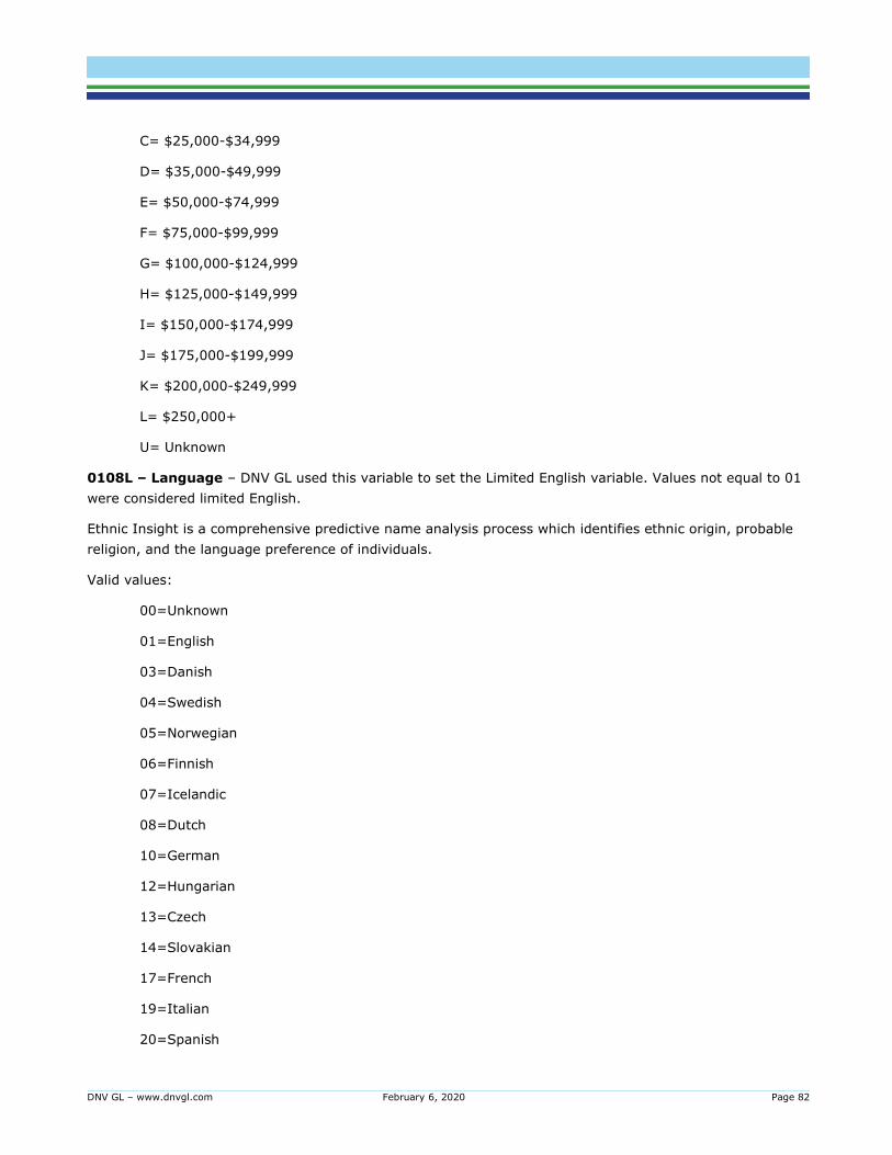
DNV GL – www.dnvgl.com February 6, 2020 Page 82
C= $25,000-$34,999
D= $35,000-$49,999
E= $50,000-$74,999
F= $75,000-$99,999
G= $100,000-$124,999
H= $125,000-$149,999
I= $150,000-$174,999
J= $175,000-$199,999
K= $200,000-$249,999
L= $250,000+
U= Unknown
0108L – Language – DNV GL used this variable to set the Limited English variable. Values not equal to 01
were considered limited English.
Ethnic Insight is a comprehensive predictive name analysis process which identifies ethnic origin, probable
religion, and the language preference of individuals.
Valid values:
00=Unknown
01=English
03=Danish
04=Swedish
05=Norwegian
06=Finnish
07=Icelandic
08=Dutch
10=German
12=Hungarian
13=Czech
14=Slovakian
17=French
19=Italian
20=Spanish

DNV GL – www.dnvgl.com February 6, 2020 Page 83
21=Portuguese
22=Polish
23=Estonian
24=Latvian
25=Lithuanian
27=Georgian
29=Armenian
30=Russian
31=Turkish
33=Greek
34=Farsi
35=Moldavian
36=Bulgarian
37=Romanian
38=Albanian
40=Slovenian
41=Serbo-Croatian
44=Azeri
45=Kazakh
46=Pashto
47=Urdu
48=Bengali
49=Indonesian
51=Burmese
52=Mongolian
53=Mandarin
54=Cantonese
56=Korean
57=Japanese
58=Thai

DNV GL – www.dnvgl.com February 6, 2020 Page 84
59=Malay
60=Laotian (Include Hmong)
61=Khmer
62=Vietnamese
63=Sinhalese
64=Uzbeki
65=Hmong
68=Hebrew
70=Arabic
72=Turkmeni
73=Tajik
74=Kirghiz
7E=Nepali
7F=Samoan
80=Tongan
86=Oromo
88=Gha
8G=Tibetan
8I=Swazi
8J=Zulu
8K=Xhosa
8M=Afrikaans
8O=Comorian
8S=Ashanti
8T=Swahili
8X=Hausa
92=Bantu
94=Dzongha
95=Amharic
97=Twswan

DNV GL – www.dnvgl.com February 6, 2020 Page 85
9E=Somali
9F=Macedonian
9N=Tagalog
9O=Sotho
9R=Malagasy
9S=Basque

DNV GL – www.dnvgl.com February 6, 2020 Page 86
7 APPENDIX B: LOW PARTICIPATION TABLE
Overview of Community Outreach Metric for 2017 Residential Nonparticipant Customer Profile
Study (MA19X06-B-RESNONPART)
This appendix provides a brief description of the Community Outreach Metric added to the Low Participation
Table for the 2017 Residential Nonparticipant Customer Profile Study (RNCPS). An embedded copy of the
Excel file with the table appears at the end of the appendix.
Community Outreach Metric formulation
Figure 7-1 shows how to calculate the Community Outreach Metric, along with its key features:
Figure 7-1. Community Outreach Metric formula and features3334
We calculate the Community Outreach Metric by taking the sum of the proportion of households matching
each term sheet variable, and dividing it by the account participation rate. We compute and report this
metric at both the block group level and the town level (as categorized by the Massachusetts State Tax
Assessor).
Key features of the Community Outreach Metric include:
• It looks at each block group as an independent point within an absolute data range of 0% to 100% for
each term sheet characteristic. This makes it easy to identify block groups with high proportions of one
or more term sheet characteristics. However, because the block groups are independent, this metric
does not show how block groups compare with one another in terms of high or low proportions of term
sheet characteristics.
• Its numerator is based on the term sheet characteristics. This means that the metric’s numeric value
increases as the prevalence of the term sheet characteristics increases. Households get counted once for
each characteristic they exhibit. For example, a renting, moderate-income household with limited
English (matching 3 of the term sheet characteristics) would be counted 3 times in the numerator.
• Its denominator is based on historic participation rates. By capturing historic participation in the
denominator, the metric’s numeric value is lower for communities that already have high participation
levels.
• The metric does not depend on community size. This puts small and large communities on equal footing
and gives program implementers the option to consider community population size separately from
other factors.
33 Census block groups are discreet, usually small, geographic areas. Since they are discreet and non-overlapping, data counts (e.g., number of low
income homes) can be aggregated and summed to less detailed geographic areas (e.g., a city, MSA, or county) and can be recombined to reflect non-standard areas (e.g., a CAP’s service zip codes, or informal neighborhoods) without having to restructure the data.
34 Deliverable 1 was an Excel workbook organized by block group and town. It listed the proportion of households in each block group (town) that
meet the three term sheet characteristics and that live in multifamily buildings. It also listed consumption-weighted location participation for
each block group. The tables are dynamic, allowing users to restrict the table to any permutation of PA territories.
��%�������, %��*�����. ������, %������*. ������ℎ"
#����� ����������� ����
Considers each block group2 individually
Households matching multiple term sheet characteristics count multiple times
Can be weighted to reflect different priorities by community or program year
Can be calculated directly from Deliverable 13

DNV GL – www.dnvgl.com February 6, 2020 Page 87
• The PAs can easily update the metric by updating the ACS data and the PAs’ data in future years.
Key limitations of the metric include:
• In communities with smaller populations, the measurements of the term sheet characteristics and
participation rates are more sensitive to small changes. The denominators in these measurements
represent the entire population. When those denominators are small, small changes in the numerators
have stronger effects on the resulting measurement. For example, a difference of 10 renters would
cause a 1% change in the renter proportion for a block group with 1,000 homes, but it would cause a
10% change in the renter proportion for a block group with 100 homes.
• Account participation rate is calculated by dividing the total number of unique account IDs that
participated from 2013 to 2017 (unique across the entire period) by the total number of unique (across
the entire period) billed account ids from 2013 to 2017. The two primary drawbacks of using account
participation are that it can fail to fully represent participation in master-metered multifamily buildings,
and it underrepresents participation in time-series analyses. Master-metered multifamily buildings count
as a single account in the metric, even if multiple residences were treated by the programs. Account ids
change every time someone moves in or out of a premise. This means the denominator of account
participation rate will tend to increase faster than the numerator because new residents have a less than
100% probability to participate in a program.
Data Quality Checks
DNV GL verified that the Community Outreach Metric correlates positively with the proportions of each block
group that matches the term sheet variables. The Community Outreach Metric also correlates negatively
with the historic account participation rate.
We examined the 5 highest and 5 lowest scoring towns in greater depth. We verified that these towns match
areas that the bivariate maps (Appendix C) identify as areas of low participation and high term sheet
characteristics. Furthermore, we examined why each of the 5 highest and 5 lowest scoring towns scored
how it did. For the towns with the highest scores, the deciding factors were low participation (small
denominator) and high renter population (large numerator). For the towns with the lowest scores, the
deciding factors were moderate participation rate (moderately large denominator) and low renter
population, low moderate-income population, and low limited-English-speaking population (extremely small
numerator). Table 7-1 provides more detail.

DNV GL – www.dnvgl.com February 6, 2020 Page 88
Table 7-1. Highest and lowest scoring town analysis
High metric
towns
Numerator Denominator
Town Renter
%
Moderate
income %
Limited
English %
Dual Fuel Participation
rate
LAWRENCE 70% 15% 25% 6%
FALL RIVER 65% 17% 9% 6%
FITCHBURG 48% 14% 5% 6%
NEW BEDFORD 58% 16% 13% 8%
CHELSEA 74% 17% 27% 11%
Low metric
towns Numerator Denominator
Town Renter
%
Moderate
income %
Limited
English %
Dual Fuel Participation
rate
BOLTON 4% 1% 0% 37%
CARLISLE 4% 3% 1% 36%
HINGHAM 3% 3% 0% 22%
NORFOLK 5% 6% 0% 39%
BOXFORD 2% 8% 1% 35%
DNV GL provided the community outreach metric deliverable to the PAs in a dynamic Excel file. The
following tables provide the top-level content included in that deliverable. The Excel file provided additional
functionality to sort, slice, and drill down into the block group level under each town. This functionality is not
possible to reproduce in a static document.

DNV GL – www.dnvgl.com February 6, 2020 Page 89
Table 7-2. Community outreach metric table: Dual-fuel
Town
Ratio of
MF/Total
Units
Ratio
Renter
Occupied
Units
(ACS)
Ratio of
Households
at 56 - 85%
of
Statewide
Median
Income
(ACS)
Ratio
Limited
English
Speaking
Households
Unweighted
Participation
Rate
Gas &
Electric
Combined
2013-2017
Consumption
Weighted
Participation
Rate
(Mmbtu)
Electric
Combined
2013-2017
Consumption
Weighted
Participation
Rate (KWh)
Gas
Combined
2013-2017
Consumption
Weighted
Participation
Rate
(Therms)
Dual Fuel
Participants
Combined
2013-2017
Dual Fuel
Locations
Combined
2013-
2017
Community
Outreach
Metric
ABINGTON 21% 32% 17% 1% 21% 39% 41% 37% 375 2031 2.39
ACTON 23% 23% 7% 3% 27% 46% 47% 46% 1074 3484 1.24
ACUSHNET 3% 12% 13% 2% 22% 25% 31% 21% 252 1829 1.22
ADAMS 16% 33% 21% 1% 19% 24% 33% 20% 287 1710 2.81
AGAWAM 22% 26% 17% 2% 18% 30% 35% 28% 659 5962 2.45
AMESBURY 23% 31% 13% 0% 17% 33% 35% 32% 620 3139 2.58
AMHERST 35% 55% 11% 3% 13% 36% 38% 33% 207 1245 5.42
ANDOVER 18% 20% 9% 4% 21% 34% 41% 30% 771 6013 1.54
ARLINGTON 22% 39% 9% 3% 22% 38% 42% 36% 2259 9704 2.37
ASHBY 0% 12% 9% 0% 18% 22% 21% 25% 18 123 1.12
ASHLAND 8% 20% 10% 3% 28% 48% 50% 47% 816 3146 1.18
ATTLEBORO 14% 35% 14% 3% 15% 25% 30% 20% 432 5584 3.48
AUBURN 7% 19% 14% 1% 26% 38% 44% 30% 143 805 1.25
AVON 5% 26% 19% 2% 18% 21% 31% 15% 39 691 2.61
AYER 18% 35% 18% 2% 19% 33% 39% 29% 207 1205 2.94
BARNSTABLE 8% 25% 16% 3% 20% 25% 34% 21% 1921 17133 2.26
BEDFORD 20% 29% 9% 4% 34% 46% 46% 46% 835 2947 1.22
BELLINGHAM 13% 21% 10% 3% 22% 29% 35% 25% 179 1520 1.59
BERLIN 1% 16% 8% 0% 25% 41% 33% 62% 9 77 0.98
BEVERLY 26% 42% 12% 1% 19% 32% 34% 31% 1336 6222 2.88
BILLERICA 14% 18% 11% 2% 24% 34% 32% 36% 1842 8648 1.30
BOLTON 0% 4% 1% 0% 37% 44% 45% 32% 6 29 0.15
BOSTON 40% 63% 13% 12% 12% 29% 38% 26% 12700 77783 7.43

DNV GL – www.dnvgl.com February 6, 2020 Page 90
Town
Ratio of
MF/Total
Units
Ratio
Renter
Occupied
Units
(ACS)
Ratio of
Households
at 56 - 85%
of
Statewide
Median
Income
(ACS)
Ratio
Limited
English
Speaking
Households
Unweighted
Participation
Rate
Gas &
Electric
Combined
2013-2017
Consumption
Weighted
Participation
Rate
(Mmbtu)
Electric
Combined
2013-2017
Consumption
Weighted
Participation
Rate (KWh)
Gas
Combined
2013-2017
Consumption
Weighted
Participation
Rate
(Therms)
Dual Fuel
Participants
Combined
2013-2017
Dual Fuel
Locations
Combined
2013-
2017
Community
Outreach
Metric
BOURNE 6% 23% 12% 1% 18% 25% 32% 21% 503 5248 2.01
BOXFORD 2% 2% 8% 1% 35% 42% 40% 43% 372 1209 0.29
BOYLSTON 0% 13% 7% 0% 12% 55% 100% 41% 0 0 1.71
BREWSTER 7% 16% 16% 0% 23% 31% 40% 25% 274 2584 1.37
BRIDGEWATER 14% 25% 11% 2% 18% 26% 35% 19% 218 2819 2.07
BROCKTON 20% 45% 16% 11% 11% 18% 26% 14% 655 13700 6.74
BROOKFIELD 4% 44% 30% 0% 18% 23% 31% 17% 13 94 4.15
BROOKLINE 52% 51% 8% 7% 10% 31% 32% 31% 1294 7239 6.70
BURLINGTON 29% 30% 12% 5% 27% 44% 48% 41% 880 3475 1.74
CAMBRIDGE 53% 62% 10% 6% 8% 30% 39% 27% 1975 14138 9.63
CANTON 23% 22% 11% 4% 21% 34% 42% 30% 568 4162 1.74
CARLISLE 2% 4% 3% 1% 36% 41% 40% 41% 207 709 0.23
CARVER 1% 10% 11% 0% 25% 36% 40% 33% 207 1229 0.85
CHATHAM 3% 20% 12% 0% 16% 19% 24% 17% 304 4677 2.06
CHELMSFORD 18% 17% 11% 2% 30% 44% 40% 46% 2704 8701 0.99
CHELSEA 40% 74% 17% 27% 11% 22% 36% 17% 288 3614 10.34
CHESHIRE 1% 22% 25% 0% 20% 32% 31% 33% 38 320 2.34
CHICOPEE 0% 14% 6% 6% 9% 16% 62% 15% 0 0 2.82
CLARKSBURG 2% 15% 23% 0% 22% 22% 22% 22% 10 186 1.70
CLINTON 21% 46% 18% 3% 16% 32% 34% 31% 274 1696 4.30
COHASSET 8% 20% 9% 0% 27% 37% 42% 34% 350 1478 1.09
CONCORD 1% 6% 4% 0% 31% 36% 67% 36% 5 12 0.30
DALTON 5% 24% 18% 1% 22% 30% 37% 27% 226 1380 1.97
DARTMOUTH 11% 24% 15% 3% 21% 26% 32% 24% 824 6129 2.02

DNV GL – www.dnvgl.com February 6, 2020 Page 91
Town
Ratio of
MF/Total
Units
Ratio
Renter
Occupied
Units
(ACS)
Ratio of
Households
at 56 - 85%
of
Statewide
Median
Income
(ACS)
Ratio
Limited
English
Speaking
Households
Unweighted
Participation
Rate
Gas &
Electric
Combined
2013-2017
Consumption
Weighted
Participation
Rate
(Mmbtu)
Electric
Combined
2013-2017
Consumption
Weighted
Participation
Rate (KWh)
Gas
Combined
2013-2017
Consumption
Weighted
Participation
Rate
(Therms)
Dual Fuel
Participants
Combined
2013-2017
Dual Fuel
Locations
Combined
2013-
2017
Community
Outreach
Metric
DEDHAM 17% 32% 12% 2% 23% 32% 37% 30% 1268 6520 2.07
DEERFIELD 3% 26% 16% 0% 24% 30% 33% 26% 42 349 1.74
DENNIS 8% 21% 18% 2% 18% 24% 33% 20% 867 9092 2.29
DIGHTON 6% 12% 13% 1% 17% 27% 41% 15% 25 373 1.49
DOVER 0% 4% 7% 1% 33% 44% 43% 45% 6 26 0.34
DRACUT 20% 23% 13% 1% 19% 36% 38% 36% 1297 6515 1.95
DUDLEY 9% 24% 17% 2% 20% 28% 34% 14% 57 531 2.16
DUNSTABLE 0% 3% 10% 1% 29% 35% 37% 32% 71 310 0.45
DUXBURY 6% 11% 7% 0% 25% 31% 39% 27% 346 2886 0.72
EAST BRIDGEWATER 7% 17% 15% 1% 21% 19% 16% 22% 168 1885 1.57
EAST BROOKFIELD 2% 16% 14% 0% 21% 13% 16% 9% 16 110 1.39
EAST LONGMEADOW 9% 16% 11% 2% 25% 22% 12% 27% 585 4189 1.16
EASTHAM 0% 15% 15% 0% 20% 24% 29% 21% 180 2173 1.51
EASTHAMPTON 20% 44% 16% 1% 17% 31% 41% 23% 207 2282 3.53
EASTON 11% 18% 11% 1% 22% 31% 39% 25% 299 2942 1.41
ESSEX 9% 22% 15% 1% 20% 32% 31% 33% 87 487 1.88
EVERETT 16% 61% 20% 16% 9% 18% 27% 16% 715 8276 10.33
FAIRHAVEN 11% 26% 13% 2% 18% 26% 29% 25% 659 4896 2.33
FALL RIVER 30% 65% 17% 9% 6% 13% 20% 11% 878 16484 15.07
FALMOUTH 6% 22% 13% 1% 18% 24% 29% 22% 1161 11988 1.98
FITCHBURG 17% 48% 14% 5% 6% 19% 27% 16% 342 6877 11.96
FOXBOROUGH 23% 34% 9% 1% 20% 30% 33% 29% 401 3243 2.16
FRAMINGHAM 27% 43% 13% 12% 21% 36% 41% 34% 2101 10188 3.15
FRANKLIN 16% 19% 10% 1% 22% 34% 41% 31% 884 5971 1.35

DNV GL – www.dnvgl.com February 6, 2020 Page 92
Town
Ratio of
MF/Total
Units
Ratio
Renter
Occupied
Units
(ACS)
Ratio of
Households
at 56 - 85%
of
Statewide
Median
Income
(ACS)
Ratio
Limited
English
Speaking
Households
Unweighted
Participation
Rate
Gas &
Electric
Combined
2013-2017
Consumption
Weighted
Participation
Rate
(Mmbtu)
Electric
Combined
2013-2017
Consumption
Weighted
Participation
Rate (KWh)
Gas
Combined
2013-2017
Consumption
Weighted
Participation
Rate
(Therms)
Dual Fuel
Participants
Combined
2013-2017
Dual Fuel
Locations
Combined
2013-
2017
Community
Outreach
Metric
FREETOWN 0% 15% 12% 1% 26% 32% 33% 28% 27 233 1.04
GARDNER 28% 53% 18% 2% 13% 29% 33% 22% 40 660 5.63
GEORGETOWN 13% 20% 25% 0% 22% 22% 70% 21% 3 1 2.10
GLOUCESTER 12% 37% 14% 3% 19% 31% 35% 29% 844 4679 2.88
GRAFTON 12% 28% 13% 1% 23% 38% 34% 41% 552 2604 1.81
GRANBY 11% 19% 5% 0% 27% 29% 32% 23% 17 204 0.87
GREAT BARRINGTON 18% 35% 22% 5% 17% 20% 11% 28% 58 560 3.51
GREENFIELD 20% 46% 16% 2% 18% 33% 42% 26% 324 2405 3.54
GROTON 0% 5% 15% 0% 24% 33% 8% 33% 0 0 0.80
HADLEY 13% 27% 23% 2% 24% 40% 48% 32% 52 355 2.18
HALIFAX 3% 10% 15% 2% 27% 32% 36% 27% 42 633 0.99
HAMILTON 10% 17% 9% 3% 26% 24% 15% 35% 198 853 1.11
HAMPDEN 2% 8% 14% 1% 30% 33% 37% 29% 179 749 0.76
HANOVER 7% 14% 11% 2% 24% 31% 36% 27% 263 2343 1.11
HANSON 2% 9% 8% 1% 24% 29% 34% 25% 169 1783 0.75
HARVARD 3% 7% 5% 0% 35% 46% 45% 47% 48 179 0.35
HARWICH 7% 15% 15% 1% 20% 24% 33% 21% 576 6071 1.53
HATFIELD 8% 25% 19% 0% 22% 36% 42% 32% 71 507 2.03
HAVERHILL 23% 41% 15% 4% 14% 27% 28% 26% 1915 12228 4.10
HINGHAM 0% 3% 3% 0% 22% 33% 21% 33% 1 26 0.27
HOLBROOK 11% 20% 15% 2% 18% 26% 36% 19% 125 1640 2.04
HOLLISTON 10% 15% 9% 1% 35% 41% 46% 38% 694 2913 0.74
HOPEDALE 5% 21% 10% 3% 28% 39% 44% 30% 46 321 1.23
HOPKINTON 5% 15% 7% 2% 29% 47% 50% 45% 696 2407 0.83

DNV GL – www.dnvgl.com February 6, 2020 Page 93
Town
Ratio of
MF/Total
Units
Ratio
Renter
Occupied
Units
(ACS)
Ratio of
Households
at 56 - 85%
of
Statewide
Median
Income
(ACS)
Ratio
Limited
English
Speaking
Households
Unweighted
Participation
Rate
Gas &
Electric
Combined
2013-2017
Consumption
Weighted
Participation
Rate
(Mmbtu)
Electric
Combined
2013-2017
Consumption
Weighted
Participation
Rate (KWh)
Gas
Combined
2013-2017
Consumption
Weighted
Participation
Rate
(Therms)
Dual Fuel
Participants
Combined
2013-2017
Dual Fuel
Locations
Combined
2013-
2017
Community
Outreach
Metric
HUDSON 0% 0% 13% 3% 29% 33% 100% 33% 3 0 0.58
IPSWICH 23% 30% 16% 2% 17% 33% 20% 33% 1 0 2.71
KINGSTON 11% 23% 10% 0% 26% 41% 44% 38% 268 1343 1.30
LANCASTER 3% 19% 15% 3% 26% 36% 36% 39% 23 160 1.37
LANESBOROUGH 12% 15% 17% 0% 14% 19% 17% 21% 4 164 2.17
LAWRENCE 25% 70% 15% 25% 6% 14% 26% 11% 414 10031 18.57
LEE 17% 30% 16% 3% 17% 27% 29% 26% 127 1225 2.79
LEICESTER 10% 32% 17% 4% 26% 38% 39% 27% 15 99 2.02
LENOX 30% 40% 19% 2% 18% 33% 32% 34% 145 1050 3.38
LEOMINSTER 26% 45% 14% 6% 19% 35% 43% 27% 710 4178 3.40
LEXINGTON 13% 19% 7% 4% 34% 45% 47% 43% 1268 4783 0.88
LINCOLN 13% 19% 7% 2% 36% 41% 44% 39% 187 734 0.76
LONGMEADOW 6% 9% 9% 4% 28% 33% 38% 31% 832 4863 0.79
LOWELL 36% 58% 16% 14% 11% 23% 29% 21% 2410 16682 8.12
LUDLOW 10% 25% 15% 7% 18% 30% 36% 25% 362 3452 2.59
LUNENBURG 7% 22% 15% 1% 18% 33% 34% 32% 41 465 2.07
LYNN 28% 56% 14% 15% 12% 22% 28% 19% 1855 14888 7.39
MALDEN 33% 59% 13% 16% 14% 28% 32% 26% 1453 9147 6.23
MANCHESTER 12% 31% 10% 1% 22% 31% 31% 32% 245 1196 1.90
MARION 6% 23% 17% 0% 21% 26% 31% 24% 107 770 1.86
MARLBOROUGH 30% 45% 14% 11% 17% 34% 37% 32% 1185 6727 4.20
MARSHFIELD 12% 22% 11% 1% 19% 27% 34% 25% 605 6800 1.72
MASHPEE 8% 13% 14% 1% 19% 29% 39% 25% 682 6436 1.44
MATTAPOISETT 1% 19% 18% 0% 22% 30% 37% 26% 183 1181 1.67

DNV GL – www.dnvgl.com February 6, 2020 Page 94
Town
Ratio of
MF/Total
Units
Ratio
Renter
Occupied
Units
(ACS)
Ratio of
Households
at 56 - 85%
of
Statewide
Median
Income
(ACS)
Ratio
Limited
English
Speaking
Households
Unweighted
Participation
Rate
Gas &
Electric
Combined
2013-2017
Consumption
Weighted
Participation
Rate
(Mmbtu)
Electric
Combined
2013-2017
Consumption
Weighted
Participation
Rate (KWh)
Gas
Combined
2013-2017
Consumption
Weighted
Participation
Rate
(Therms)
Dual Fuel
Participants
Combined
2013-2017
Dual Fuel
Locations
Combined
2013-
2017
Community
Outreach
Metric
MAYNARD 11% 28% 10% 0% 22% 37% 39% 36% 421 2177 1.79
MEDFIELD 9% 12% 6% 0% 30% 36% 46% 31% 405 2475 0.60
MEDFORD 21% 44% 13% 7% 16% 31% 38% 29% 2147 13563 3.96
MEDWAY 9% 15% 6% 1% 26% 32% 42% 26% 265 2143 0.80
MELROSE 26% 33% 14% 3% 24% 38% 43% 37% 1420 5965 2.11
MENDON 0% 11% 3% 0% 35% 41% 42% 35% 13 58 0.42
METHUEN 18% 29% 14% 6% 13% 26% 30% 24% 711 9715 3.70
MILFORD 16% 32% 16% 5% 20% 32% 37% 29% 525 3521 2.66
MILLBURY 12% 27% 12% 2% 25% 40% 46% 32% 221 1177 1.59
MILLIS 9% 19% 13% 0% 25% 35% 41% 29% 144 983 1.28
MILTON 10% 17% 8% 1% 30% 37% 41% 36% 1453 6376 0.89
MONSON 5% 24% 22% 0% 27% 33% 33% 38% 106 61 1.71
MONTAGUE 16% 48% 17% 2% 17% 28% 36% 19% 56 617 3.99
NAHANT 16% 32% 15% 1% 20% 28% 26% 29% 205 1216 2.33
NATICK 24% 27% 13% 3% 25% 43% 47% 40% 1371 6049 1.71
NEEDHAM 12% 17% 8% 3% 29% 40% 41% 39% 1174 5380 0.94
NEW BEDFORD 20% 58% 16% 13% 8% 16% 24% 15% 1893 23265 10.77
NEW MARLBOROUGH 1% 12% 15% 0% 14% 19% 18% 100% 1 1 1.91
NEWBURY 5% 15% 10% 1% 23% 27% 26% 29% 97 497 1.12
NEWBURYPORT 18% 26% 12% 0% 21% 40% 43% 39% 1151 4417 1.83
NEWTON 15% 29% 8% 5% 24% 38% 41% 37% 4804 21917 1.74
NORFOLK 2% 5% 6% 0% 39% 44% 48% 32% 63 380 0.28
NORTH ADAMS 18% 46% 15% 2% 17% 27% 35% 24% 393 2372 3.74
NORTH ANDOVER 23% 27% 9% 1% 21% 33% 40% 29% 549 4731 1.73
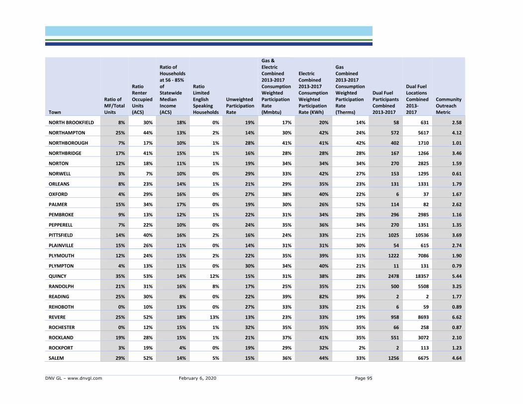
DNV GL – www.dnvgl.com February 6, 2020 Page 95
Town
Ratio of
MF/Total
Units
Ratio
Renter
Occupied
Units
(ACS)
Ratio of
Households
at 56 - 85%
of
Statewide
Median
Income
(ACS)
Ratio
Limited
English
Speaking
Households
Unweighted
Participation
Rate
Gas &
Electric
Combined
2013-2017
Consumption
Weighted
Participation
Rate
(Mmbtu)
Electric
Combined
2013-2017
Consumption
Weighted
Participation
Rate (KWh)
Gas
Combined
2013-2017
Consumption
Weighted
Participation
Rate
(Therms)
Dual Fuel
Participants
Combined
2013-2017
Dual Fuel
Locations
Combined
2013-
2017
Community
Outreach
Metric
NORTH BROOKFIELD 8% 30% 18% 0% 19% 17% 20% 14% 58 631 2.58
NORTHAMPTON 25% 44% 13% 2% 14% 30% 42% 24% 572 5617 4.12
NORTHBOROUGH 7% 17% 10% 1% 28% 41% 41% 42% 402 1710 1.01
NORTHBRIDGE 17% 41% 15% 1% 16% 28% 28% 28% 167 1266 3.46
NORTON 12% 18% 11% 1% 19% 34% 34% 34% 270 2825 1.59
NORWELL 3% 7% 10% 0% 29% 33% 42% 27% 153 1295 0.61
ORLEANS 8% 23% 14% 1% 21% 29% 35% 23% 131 1331 1.79
OXFORD 4% 29% 16% 0% 27% 38% 40% 22% 6 37 1.67
PALMER 15% 34% 17% 0% 19% 30% 26% 52% 114 82 2.62
PEMBROKE 9% 13% 12% 1% 22% 31% 34% 28% 296 2985 1.16
PEPPERELL 7% 22% 10% 0% 24% 35% 36% 34% 270 1351 1.35
PITTSFIELD 14% 40% 16% 2% 16% 24% 33% 21% 1025 10536 3.69
PLAINVILLE 15% 26% 11% 0% 14% 31% 31% 30% 54 615 2.74
PLYMOUTH 12% 24% 15% 2% 22% 35% 39% 31% 1222 7086 1.90
PLYMPTON 4% 13% 11% 0% 30% 34% 40% 21% 11 131 0.79
QUINCY 35% 53% 14% 12% 15% 31% 38% 28% 2478 18357 5.44
RANDOLPH 21% 31% 16% 8% 17% 25% 35% 21% 500 5508 3.25
READING 25% 30% 8% 0% 22% 39% 82% 39% 2 2 1.77
REHOBOTH 0% 10% 13% 0% 27% 33% 33% 21% 6 59 0.89
REVERE 25% 52% 18% 13% 13% 23% 33% 19% 958 8693 6.62
ROCHESTER 0% 12% 15% 1% 32% 35% 35% 35% 66 258 0.87
ROCKLAND 19% 28% 15% 1% 21% 37% 41% 35% 551 3072 2.10
ROCKPORT 3% 19% 4% 0% 19% 29% 32% 2% 2 113 1.23
SALEM 29% 52% 14% 5% 15% 36% 44% 33% 1256 6675 4.64
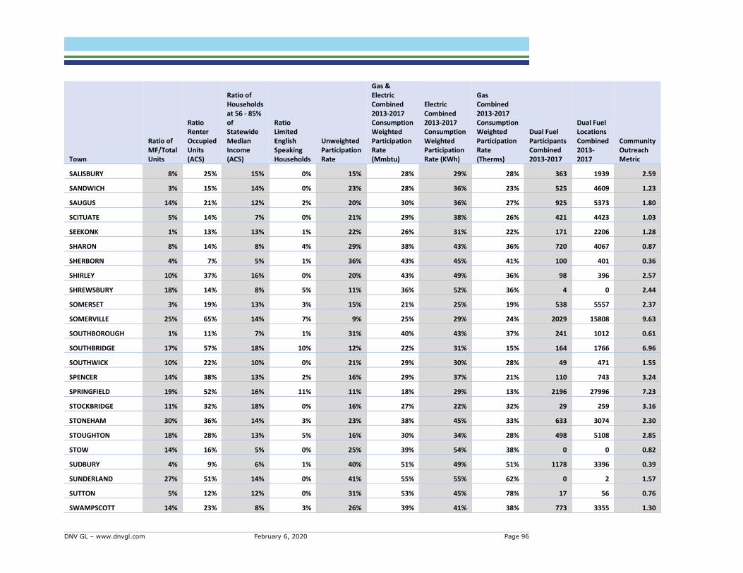
DNV GL – www.dnvgl.com February 6, 2020 Page 96
Town
Ratio of
MF/Total
Units
Ratio
Renter
Occupied
Units
(ACS)
Ratio of
Households
at 56 - 85%
of
Statewide
Median
Income
(ACS)
Ratio
Limited
English
Speaking
Households
Unweighted
Participation
Rate
Gas &
Electric
Combined
2013-2017
Consumption
Weighted
Participation
Rate
(Mmbtu)
Electric
Combined
2013-2017
Consumption
Weighted
Participation
Rate (KWh)
Gas
Combined
2013-2017
Consumption
Weighted
Participation
Rate
(Therms)
Dual Fuel
Participants
Combined
2013-2017
Dual Fuel
Locations
Combined
2013-
2017
Community
Outreach
Metric
SALISBURY 8% 25% 15% 0% 15% 28% 29% 28% 363 1939 2.59
SANDWICH 3% 15% 14% 0% 23% 28% 36% 23% 525 4609 1.23
SAUGUS 14% 21% 12% 2% 20% 30% 36% 27% 925 5373 1.80
SCITUATE 5% 14% 7% 0% 21% 29% 38% 26% 421 4423 1.03
SEEKONK 1% 13% 13% 1% 22% 26% 31% 22% 171 2206 1.28
SHARON 8% 14% 8% 4% 29% 38% 43% 36% 720 4067 0.87
SHERBORN 4% 7% 5% 1% 36% 43% 45% 41% 100 401 0.36
SHIRLEY 10% 37% 16% 0% 20% 43% 49% 36% 98 396 2.57
SHREWSBURY 18% 14% 8% 5% 11% 36% 52% 36% 4 0 2.44
SOMERSET 3% 19% 13% 3% 15% 21% 25% 19% 538 5557 2.37
SOMERVILLE 25% 65% 14% 7% 9% 25% 29% 24% 2029 15808 9.63
SOUTHBOROUGH 1% 11% 7% 1% 31% 40% 43% 37% 241 1012 0.61
SOUTHBRIDGE 17% 57% 18% 10% 12% 22% 31% 15% 164 1766 6.96
SOUTHWICK 10% 22% 10% 0% 21% 29% 30% 28% 49 471 1.55
SPENCER 14% 38% 13% 2% 16% 29% 37% 21% 110 743 3.24
SPRINGFIELD 19% 52% 16% 11% 11% 18% 29% 13% 2196 27996 7.23
STOCKBRIDGE 11% 32% 18% 0% 16% 27% 22% 32% 29 259 3.16
STONEHAM 30% 36% 14% 3% 23% 38% 45% 33% 633 3074 2.30
STOUGHTON 18% 28% 13% 5% 16% 30% 34% 28% 498 5108 2.85
STOW 14% 16% 5% 0% 25% 39% 54% 38% 0 0 0.82
SUDBURY 4% 9% 6% 1% 40% 51% 49% 51% 1178 3396 0.39
SUNDERLAND 27% 51% 14% 0% 41% 55% 55% 62% 0 2 1.57
SUTTON 5% 12% 12% 0% 31% 53% 45% 78% 17 56 0.76
SWAMPSCOTT 14% 23% 8% 3% 26% 39% 41% 38% 773 3355 1.30

DNV GL – www.dnvgl.com February 6, 2020 Page 97
Town
Ratio of
MF/Total
Units
Ratio
Renter
Occupied
Units
(ACS)
Ratio of
Households
at 56 - 85%
of
Statewide
Median
Income
(ACS)
Ratio
Limited
English
Speaking
Households
Unweighted
Participation
Rate
Gas &
Electric
Combined
2013-2017
Consumption
Weighted
Participation
Rate
(Mmbtu)
Electric
Combined
2013-2017
Consumption
Weighted
Participation
Rate (KWh)
Gas
Combined
2013-2017
Consumption
Weighted
Participation
Rate
(Therms)
Dual Fuel
Participants
Combined
2013-2017
Dual Fuel
Locations
Combined
2013-
2017
Community
Outreach
Metric
SWANSEA 2% 13% 14% 3% 17% 22% 27% 20% 429 4398 1.72
TEWKSBURY 12% 14% 10% 1% 22% 43% 41% 44% 1177 5486 1.13
TOPSFIELD 2% 8% 10% 0% 31% 38% 44% 35% 217 879 0.60
TOWNSEND 9% 20% 13% 0% 14% 19% 23% 17% 137 1553 2.35
TYNGSBOROUGH 10% 14% 13% 2% 25% 37% 35% 39% 623 2538 1.12
UPTON 7% 23% 7% 1% 26% 37% 39% 35% 126 524 1.16
UXBRIDGE 6% 22% 12% 1% 23% 40% 40% 40% 182 1005 1.54
WAKEFIELD 0% 8% 10% 3% 11% 25% 17% 52% 0 2 1.81
WALPOLE 11% 18% 11% 1% 23% 32% 40% 28% 569 4075 1.29
WALTHAM 30% 50% 13% 6% 14% 33% 35% 32% 1612 8724 5.09
WAREHAM 6% 23% 15% 1% 17% 31% 35% 29% 744 5370 2.29
WARREN 12% 37% 14% 0% 14% 19% 22% 16% 36 291 3.54
WATERTOWN 24% 49% 12% 4% 15% 35% 41% 33% 1323 7533 4.29
WAYLAND 6% 12% 4% 2% 34% 43% 44% 42% 787 2797 0.53
WEBSTER 17% 51% 19% 4% 13% 24% 31% 16% 118 1227 5.61
WENHAM 10% 12% 13% 0% 28% 38% 37% 39% 125 493 0.91
WEST BRIDGEWATER 3% 14% 16% 0% 21% 22% 19% 24% 79 1051 1.40
WEST BROOKFIELD 13% 29% 15% 0% 20% 18% 20% 16% 52 277 2.17
WEST NEWBURY 2% 4% 8% 0% 33% 42% 40% 47% 62 167 0.36
WEST SPRINGFIELD 23% 40% 18% 5% 15% 24% 33% 21% 688 6265 4.14
WESTBOROUGH 33% 39% 8% 3% 21% 44% 49% 42% 566 2446 2.39
WESTFORD 5% 11% 9% 2% 29% 43% 41% 44% 1645 5951 0.74
WESTHAMPTON 0% 9% 13% 0% 29% 32% 33% 22% 1 4 0.76
WESTMINSTER 8% 15% 5% 0% 22% 34% 34% 34% 48 244 0.91

DNV GL – www.dnvgl.com February 6, 2020 Page 98
Town
Ratio of
MF/Total
Units
Ratio
Renter
Occupied
Units
(ACS)
Ratio of
Households
at 56 - 85%
of
Statewide
Median
Income
(ACS)
Ratio
Limited
English
Speaking
Households
Unweighted
Participation
Rate
Gas &
Electric
Combined
2013-2017
Consumption
Weighted
Participation
Rate
(Mmbtu)
Electric
Combined
2013-2017
Consumption
Weighted
Participation
Rate (KWh)
Gas
Combined
2013-2017
Consumption
Weighted
Participation
Rate
(Therms)
Dual Fuel
Participants
Combined
2013-2017
Dual Fuel
Locations
Combined
2013-
2017
Community
Outreach
Metric
WESTON 7% 15% 5% 3% 30% 34% 32% 35% 680 2860 0.78
WESTPORT 4% 16% 10% 2% 16% 20% 24% 18% 270 3113 1.79
WESTWOOD 17% 13% 9% 2% 28% 41% 44% 39% 474 2065 0.85
WEYMOUTH 29% 36% 15% 2% 21% 31% 36% 28% 1571 9271 2.57
WHATELY 0% 15% 19% 2% 26% 30% 31% 25% 7 43 1.37
WHITMAN 12% 28% 14% 0% 21% 36% 36% 37% 454 2255 1.99
WILBRAHAM 4% 11% 8% 1% 29% 35% 41% 31% 544 2408 0.68
WILLIAMSTOWN 11% 27% 16% 2% 19% 28% 30% 27% 145 1083 2.37
WINCHESTER 11% 15% 8% 3% 31% 42% 43% 41% 1138 4426 0.81
WINTHROP 21% 43% 15% 4% 15% 32% 38% 30% 602 3989 4.15
WOBURN 24% 38% 14% 4% 23% 36% 41% 33% 953 4894 2.44
WORCESTER 26% 57% 16% 11% 12% 24% 33% 21% 3301 26158 7.24
WRENTHAM 7% 20% 10% 0% 23% 28% 37% 22% 116 1195 1.28
YARMOUTH 11% 21% 21% 3% 20% 26% 36% 23% 1302 10874 2.26
Grand Total 22% 40% 13% 6% 16% 30% 36% 27% 136746 924392 3.67

DNV GL – www.dnvgl.com February 6, 2020 Page 99
Table 7-3. Community outreach metric table: Gas
Town
Ratio of MF/Total
Units
Ratio Renter
Occupied
Units (ACS)
Ratio of Households at
56 - 85% of Statewide
Median Income (ACS)
Ratio Limited
English
Speaking
Households
Unweighted
Participation
Rate
Gas Combined
2013-2017
Consumption
Weighted
Participation
Rate (Therms)
Community
Outreach
Metric
ABINGTON 21% 32% 17% 1% 21% 37% 2.39
ACTON 23% 23% 7% 3% 27% 46% 1.24
ACUSHNET 3% 12% 13% 2% 22% 21% 1.22
ADAMS 16% 33% 21% 1% 19% 20% 2.81
AGAWAM 22% 26% 17% 2% 18% 28% 2.45
AMESBURY 23% 31% 13% 0% 17% 32% 2.58
AMHERST 35% 55% 11% 3% 13% 33% 5.42
ANDOVER 18% 20% 9% 4% 21% 30% 1.54
ARLINGTON 22% 39% 9% 3% 22% 36% 2.37
ASHBY 0% 12% 9% 0% 18% 25% 1.12
ASHLAND 8% 20% 10% 3% 28% 47% 1.18
ATTLEBORO 14% 35% 14% 3% 15% 20% 3.48
AUBURN 7% 19% 14% 1% 26% 30% 1.25
AVON 5% 26% 19% 2% 18% 15% 2.61
AYER 18% 35% 18% 2% 19% 29% 2.94
BARNSTABLE 8% 25% 16% 3% 20% 21% 2.26
BEDFORD 20% 29% 9% 4% 34% 46% 1.22
BELLINGHAM 13% 21% 10% 3% 22% 25% 1.59
BELMONT 7% 37% 11% 4% 20% 33% 2.62
BERKLEY 0% 0% 13% 0% 9% 16% 1.37
BERLIN 1% 16% 8% 0% 25% 62% 0.98
BEVERLY 26% 42% 12% 1% 19% 31% 2.88
BILLERICA 14% 18% 11% 2% 24% 36% 1.30
BOLTON 0% 4% 1% 0% 37% 32% 0.15
BOSTON 40% 63% 13% 12% 12% 26% 7.44

DNV GL – www.dnvgl.com February 6, 2020 Page 100
Town
Ratio of MF/Total
Units
Ratio Renter
Occupied
Units (ACS)
Ratio of Households at
56 - 85% of Statewide
Median Income (ACS)
Ratio Limited
English
Speaking
Households
Unweighted
Participation
Rate
Gas Combined
2013-2017
Consumption
Weighted
Participation
Rate (Therms)
Community
Outreach
Metric
BOURNE 6% 23% 12% 1% 18% 21% 2.01
BOXBOROUGH 38% 27% 13% 1% 34% 41% 1.19
BOXFORD 2% 2% 8% 1% 35% 43% 0.29
BOYLSTON 3% 14% 14% 1% 20% 33% 1.48
BRAINTREE 21% 30% 11% 3% 32% 37% 1.36
BREWSTER 7% 16% 16% 0% 23% 25% 1.37
BRIDGEWATER 14% 25% 11% 2% 18% 19% 2.07
BROCKTON 20% 45% 16% 11% 11% 14% 6.74
BROOKFIELD 4% 44% 30% 0% 18% 17% 4.15
BROOKLINE 52% 51% 8% 7% 10% 31% 6.70
BURLINGTON 29% 30% 12% 5% 27% 41% 1.74
CAMBRIDGE 53% 62% 10% 6% 8% 27% 9.63
CANTON 23% 22% 11% 4% 21% 30% 1.74
CARLISLE 2% 4% 3% 1% 36% 41% 0.23
CARVER 1% 10% 11% 0% 25% 33% 0.85
CHATHAM 3% 20% 12% 0% 16% 17% 2.06
CHELMSFORD 18% 17% 11% 2% 30% 46% 0.99
CHELSEA 40% 74% 17% 27% 11% 17% 10.34
CHESHIRE 1% 22% 25% 0% 20% 33% 2.34
CHICOPEE 19% 42% 18% 5% 8% 18% 7.87
CLARKSBURG 2% 15% 23% 0% 22% 22% 1.70
CLINTON 21% 46% 18% 3% 16% 31% 4.30
COHASSET 8% 20% 9% 0% 27% 34% 1.09
CONCORD 18% 23% 6% 1% 24% 37% 1.24
DALTON 5% 24% 18% 1% 22% 27% 1.97
DANVERS 22% 31% 12% 1% 15% 32% 2.97

DNV GL – www.dnvgl.com February 6, 2020 Page 101
Town
Ratio of MF/Total
Units
Ratio Renter
Occupied
Units (ACS)
Ratio of Households at
56 - 85% of Statewide
Median Income (ACS)
Ratio Limited
English
Speaking
Households
Unweighted
Participation
Rate
Gas Combined
2013-2017
Consumption
Weighted
Participation
Rate (Therms)
Community
Outreach
Metric
DARTMOUTH 11% 24% 15% 3% 21% 24% 2.02
DEDHAM 17% 32% 12% 2% 23% 30% 2.07
DEERFIELD 3% 26% 16% 0% 24% 26% 1.74
DENNIS 8% 21% 18% 2% 18% 20% 2.29
DIGHTON 6% 12% 13% 1% 17% 15% 1.49
DOVER 0% 4% 7% 1% 33% 45% 0.34
DRACUT 20% 23% 13% 1% 19% 36% 1.95
DUDLEY 9% 24% 17% 2% 20% 14% 2.16
DUNSTABLE 0% 3% 10% 1% 29% 32% 0.45
DUXBURY 6% 11% 7% 0% 25% 27% 0.72
EAST BRIDGEWATER 7% 17% 15% 1% 21% 22% 1.57
EAST BROOKFIELD 2% 16% 14% 0% 21% 9% 1.39
EAST LONGMEADOW 9% 16% 11% 2% 25% 27% 1.16
EASTHAM 0% 15% 15% 0% 20% 21% 1.51
EASTHAMPTON 20% 44% 16% 1% 17% 23% 3.53
EASTON 11% 18% 11% 1% 22% 25% 1.41
ESSEX 9% 22% 15% 1% 20% 33% 1.88
EVERETT 16% 61% 20% 16% 9% 16% 10.33
FAIRHAVEN 11% 26% 13% 2% 18% 25% 2.33
FALL RIVER 30% 65% 17% 9% 6% 11% 15.07
FALMOUTH 6% 22% 13% 1% 18% 22% 1.98
FITCHBURG 17% 48% 14% 5% 6% 16% 11.96
FOXBOROUGH 23% 34% 9% 1% 20% 29% 2.16
FRAMINGHAM 27% 43% 13% 12% 21% 34% 3.15
FRANKLIN 16% 19% 10% 1% 22% 31% 1.35
FREETOWN 0% 15% 12% 1% 26% 28% 1.04

DNV GL – www.dnvgl.com February 6, 2020 Page 102
Town
Ratio of MF/Total
Units
Ratio Renter
Occupied
Units (ACS)
Ratio of Households at
56 - 85% of Statewide
Median Income (ACS)
Ratio Limited
English
Speaking
Households
Unweighted
Participation
Rate
Gas Combined
2013-2017
Consumption
Weighted
Participation
Rate (Therms)
Community
Outreach
Metric
GARDNER 28% 53% 18% 2% 13% 22% 5.63
GEORGETOWN 9% 16% 12% 0% 27% 32% 1.07
GLOUCESTER 12% 37% 14% 3% 19% 29% 2.88
GRAFTON 12% 28% 13% 1% 23% 41% 1.81
GRANBY 11% 19% 5% 0% 27% 23% 0.87
GREAT BARRINGTON 18% 35% 22% 5% 17% 28% 3.51
GREENFIELD 20% 46% 16% 2% 18% 26% 3.54
GROTON 5% 14% 7% 1% 22% 31% 0.96
GROVELAND 6% 18% 13% 1% 22% 27% 1.50
HADLEY 13% 27% 23% 2% 24% 32% 2.18
HALIFAX 3% 10% 15% 2% 27% 27% 0.99
HAMILTON 10% 17% 9% 3% 26% 35% 1.11
HAMPDEN 2% 8% 14% 1% 30% 29% 0.76
HANOVER 7% 14% 11% 2% 24% 27% 1.11
HANSON 2% 9% 8% 1% 24% 25% 0.75
HARVARD 3% 7% 5% 0% 35% 47% 0.35
HARWICH 7% 15% 15% 1% 20% 21% 1.53
HATFIELD 8% 25% 19% 0% 22% 32% 2.03
HAVERHILL 23% 40% 15% 3% 14% 27% 4.09
HINGHAM 20% 17% 8% 0% 18% 34% 1.40
HOLBROOK 11% 20% 15% 2% 18% 19% 2.04
HOLDEN 7% 13% 11% 2% 20% 28% 1.24
HOLLISTON 10% 15% 9% 1% 35% 38% 0.74
HOPEDALE 5% 21% 10% 3% 28% 30% 1.23
HOPKINTON 5% 15% 7% 2% 29% 45% 0.83
HUDSON 18% 25% 14% 5% 15% 28% 3.01

DNV GL – www.dnvgl.com February 6, 2020 Page 103
Town
Ratio of MF/Total
Units
Ratio Renter
Occupied
Units (ACS)
Ratio of Households at
56 - 85% of Statewide
Median Income (ACS)
Ratio Limited
English
Speaking
Households
Unweighted
Participation
Rate
Gas Combined
2013-2017
Consumption
Weighted
Participation
Rate (Therms)
Community
Outreach
Metric
HULL 19% 32% 12% 1% 16% 29% 2.76
IPSWICH 14% 27% 11% 2% 18% 31% 2.17
KINGSTON 11% 23% 10% 0% 26% 38% 1.30
LAKEVILLE 13% 23% 19% 0% 3% 10% 15.56
LANCASTER 3% 19% 15% 3% 26% 39% 1.37
LANESBOROUGH 12% 15% 17% 0% 14% 21% 2.17
LAWRENCE 25% 70% 15% 25% 6% 11% 18.57
LEE 17% 30% 16% 3% 17% 26% 2.79
LEICESTER 10% 32% 17% 4% 26% 27% 2.02
LENOX 30% 40% 19% 2% 18% 34% 3.38
LEOMINSTER 26% 45% 14% 6% 19% 27% 3.40
LEXINGTON 13% 19% 7% 4% 34% 43% 0.88
LINCOLN 13% 19% 7% 2% 36% 39% 0.76
LITTLETON 7% 16% 6% 1% 22% 29% 1.06
LONGMEADOW 6% 9% 9% 4% 28% 31% 0.79
LOWELL 36% 58% 16% 14% 11% 21% 8.12
LUDLOW 10% 25% 15% 7% 18% 25% 2.59
LUNENBURG 7% 22% 15% 1% 18% 32% 2.07
LYNN 28% 56% 14% 15% 12% 19% 7.39
LYNNFIELD 13% 15% 10% 2% 19% 31% 1.43
MALDEN 33% 59% 13% 16% 14% 26% 6.23
MANCHESTER 12% 31% 10% 1% 22% 32% 1.90
MANSFIELD 22% 28% 11% 1% 15% 25% 2.76
MARBLEHEAD 6% 21% 11% 2% 21% 30% 1.60
MARION 6% 23% 17% 0% 21% 24% 1.86
MARLBOROUGH 30% 45% 14% 11% 17% 32% 4.20

DNV GL – www.dnvgl.com February 6, 2020 Page 104
Town
Ratio of MF/Total
Units
Ratio Renter
Occupied
Units (ACS)
Ratio of Households at
56 - 85% of Statewide
Median Income (ACS)
Ratio Limited
English
Speaking
Households
Unweighted
Participation
Rate
Gas Combined
2013-2017
Consumption
Weighted
Participation
Rate (Therms)
Community
Outreach
Metric
MARSHFIELD 12% 22% 11% 1% 19% 25% 1.72
MASHPEE 8% 13% 14% 1% 19% 25% 1.44
MATTAPOISETT 1% 19% 18% 0% 22% 26% 1.67
MAYNARD 11% 28% 10% 0% 22% 36% 1.79
MEDFIELD 9% 12% 6% 0% 30% 31% 0.60
MEDFORD 21% 44% 13% 7% 16% 29% 3.96
MEDWAY 9% 15% 6% 1% 26% 26% 0.80
MELROSE 26% 33% 14% 3% 24% 37% 2.11
MENDON 0% 11% 3% 0% 35% 35% 0.42
MERRIMAC 5% 13% 10% 0% 17% 25% 1.33
METHUEN 18% 29% 14% 6% 13% 24% 3.70
MIDDLEBOROUGH 6% 11% 19% 2% 5% 6% 6.28
MIDDLETON 15% 15% 6% 0% 17% 38% 1.28
MILFORD 16% 32% 16% 5% 20% 29% 2.66
MILLBURY 12% 27% 12% 2% 25% 32% 1.59
MILLIS 9% 19% 13% 0% 25% 29% 1.28
MILTON 10% 17% 8% 1% 30% 36% 0.89
MONSON 5% 24% 22% 0% 27% 38% 1.71
MONTAGUE 16% 48% 17% 2% 17% 19% 3.99
NAHANT 16% 32% 15% 1% 20% 29% 2.33
NATICK 24% 27% 13% 3% 25% 40% 1.71
NEEDHAM 12% 17% 8% 3% 29% 39% 0.94
NEW BEDFORD 20% 58% 16% 13% 8% 15% 10.77
NEW MARLBOROUGH 1% 12% 15% 0% 14% 100% 1.91
NEWBURY 5% 15% 10% 1% 23% 29% 1.12
NEWBURYPORT 18% 26% 12% 0% 21% 39% 1.83

DNV GL – www.dnvgl.com February 6, 2020 Page 105
Town
Ratio of MF/Total
Units
Ratio Renter
Occupied
Units (ACS)
Ratio of Households at
56 - 85% of Statewide
Median Income (ACS)
Ratio Limited
English
Speaking
Households
Unweighted
Participation
Rate
Gas Combined
2013-2017
Consumption
Weighted
Participation
Rate (Therms)
Community
Outreach
Metric
NEWTON 15% 29% 8% 5% 24% 37% 1.74
NORFOLK 2% 5% 6% 0% 39% 32% 0.28
NORTH ADAMS 18% 46% 15% 2% 17% 24% 3.74
NORTH ANDOVER 23% 27% 9% 1% 21% 29% 1.73
NORTH ATTLEBOROUGH 18% 30% 14% 1% 8% 18% 5.85
NORTH BROOKFIELD 8% 30% 18% 0% 19% 14% 2.58
NORTH READING 12% 13% 12% 1% 18% 32% 1.46
NORTHAMPTON 25% 44% 13% 2% 14% 24% 4.12
NORTHBOROUGH 7% 17% 10% 1% 28% 42% 1.01
NORTHBRIDGE 17% 41% 15% 1% 16% 28% 3.46
NORTON 12% 18% 11% 1% 19% 34% 1.59
NORWELL 3% 7% 10% 0% 29% 27% 0.61
NORWOOD 26% 42% 11% 4% 13% 29% 4.39
ORLEANS 8% 23% 14% 1% 21% 23% 1.79
OXFORD 4% 29% 16% 0% 27% 22% 1.67
PALMER 15% 34% 17% 0% 19% 52% 2.62
PEABODY 26% 35% 17% 4% 14% 26% 4.15
PEMBROKE 9% 13% 12% 1% 22% 28% 1.16
PEPPERELL 7% 22% 10% 0% 24% 34% 1.35
PITTSFIELD 14% 39% 16% 2% 16% 22% 3.65
PLAINVILLE 15% 26% 11% 0% 14% 30% 2.74
PLYMOUTH 12% 24% 15% 2% 22% 31% 1.90
PLYMPTON 4% 13% 11% 0% 30% 21% 0.79
QUINCY 35% 53% 14% 12% 15% 28% 5.44
RANDOLPH 21% 31% 16% 8% 17% 21% 3.25
RAYNHAM 19% 23% 12% 1% 13% 21% 2.73

DNV GL – www.dnvgl.com February 6, 2020 Page 106
Town
Ratio of MF/Total
Units
Ratio Renter
Occupied
Units (ACS)
Ratio of Households at
56 - 85% of Statewide
Median Income (ACS)
Ratio Limited
English
Speaking
Households
Unweighted
Participation
Rate
Gas Combined
2013-2017
Consumption
Weighted
Participation
Rate (Therms)
Community
Outreach
Metric
READING 17% 21% 9% 1% 22% 38% 1.36
REHOBOTH 0% 10% 13% 0% 27% 21% 0.89
REVERE 25% 52% 18% 13% 13% 19% 6.62
ROCHESTER 0% 12% 15% 1% 32% 35% 0.87
ROCKLAND 19% 28% 15% 1% 21% 35% 2.10
ROCKPORT 3% 19% 4% 0% 19% 2% 1.23
ROWLEY 13% 17% 10% 0% 20% 32% 1.34
SALEM 29% 52% 14% 5% 15% 33% 4.64
SALISBURY 8% 25% 15% 0% 15% 28% 2.59
SANDWICH 3% 15% 14% 0% 23% 23% 1.23
SAUGUS 14% 21% 12% 2% 20% 27% 1.80
SCITUATE 5% 14% 7% 0% 21% 26% 1.03
SEEKONK 1% 13% 13% 1% 22% 22% 1.28
SHARON 8% 14% 8% 4% 29% 36% 0.87
SHERBORN 4% 7% 5% 1% 36% 41% 0.36
SHIRLEY 10% 37% 16% 0% 20% 36% 2.57
SHREWSBURY 21% 26% 11% 7% 18% 30% 2.48
SOMERSET 3% 19% 13% 3% 15% 19% 2.37
SOMERVILLE 25% 65% 14% 7% 9% 24% 9.63
SOUTH HADLEY 14% 26% 16% 1% 14% 28% 3.04
SOUTHBOROUGH 1% 11% 7% 1% 31% 37% 0.61
SOUTHBRIDGE 17% 57% 18% 10% 12% 15% 6.96
SOUTHWICK 10% 22% 10% 0% 21% 28% 1.55
SPENCER 14% 38% 13% 2% 16% 21% 3.24
SPRINGFIELD 19% 52% 16% 11% 11% 13% 7.23
STERLING 3% 15% 13% 0% 57% 59% 0.49

DNV GL – www.dnvgl.com February 6, 2020 Page 107
Town
Ratio of MF/Total
Units
Ratio Renter
Occupied
Units (ACS)
Ratio of Households at
56 - 85% of Statewide
Median Income (ACS)
Ratio Limited
English
Speaking
Households
Unweighted
Participation
Rate
Gas Combined
2013-2017
Consumption
Weighted
Participation
Rate (Therms)
Community
Outreach
Metric
STOCKBRIDGE 11% 32% 18% 0% 16% 32% 3.16
STONEHAM 30% 36% 14% 3% 23% 33% 2.30
STOUGHTON 18% 28% 13% 5% 16% 28% 2.85
STOW 4% 10% 8% 0% 24% 30% 0.73
SUDBURY 4% 9% 6% 1% 40% 51% 0.39
SUNDERLAND 27% 51% 14% 0% 41% 62% 1.57
SUTTON 5% 12% 12% 0% 31% 78% 0.76
SWAMPSCOTT 14% 23% 8% 3% 26% 38% 1.30
SWANSEA 2% 13% 14% 3% 17% 20% 1.72
TAUNTON 16% 38% 17% 5% 5% 14% 11.26
TEWKSBURY 12% 14% 10% 1% 22% 44% 1.13
TOPSFIELD 2% 8% 10% 0% 31% 35% 0.60
TOWNSEND 9% 20% 13% 0% 14% 17% 2.35
TYNGSBOROUGH 10% 14% 13% 2% 25% 39% 1.12
UPTON 7% 23% 7% 1% 26% 35% 1.16
UXBRIDGE 6% 22% 12% 1% 23% 40% 1.54
WAKEFIELD 10% 15% 15% 2% 18% 10% 1.81
WALPOLE 11% 18% 11% 1% 23% 28% 1.29
WALTHAM 30% 50% 13% 6% 14% 32% 5.09
WAREHAM 6% 23% 15% 1% 17% 29% 2.29
WARREN 12% 37% 14% 0% 14% 16% 3.54
WATERTOWN 24% 49% 12% 4% 15% 33% 4.29
WAYLAND 6% 12% 4% 2% 34% 42% 0.53
WEBSTER 17% 51% 19% 4% 13% 16% 5.61
WELLESLEY 11% 17% 5% 2% 31% 33% 0.79
WENHAM 10% 12% 13% 0% 28% 39% 0.91

DNV GL – www.dnvgl.com February 6, 2020 Page 108
Town
Ratio of MF/Total
Units
Ratio Renter
Occupied
Units (ACS)
Ratio of Households at
56 - 85% of Statewide
Median Income (ACS)
Ratio Limited
English
Speaking
Households
Unweighted
Participation
Rate
Gas Combined
2013-2017
Consumption
Weighted
Participation
Rate (Therms)
Community
Outreach
Metric
WEST BOYLSTON 6% 16% 14% 2% 22% 31% 1.43
WEST BRIDGEWATER 3% 14% 16% 0% 21% 24% 1.40
WEST BROOKFIELD 13% 29% 15% 0% 20% 16% 2.17
WEST NEWBURY 2% 4% 8% 0% 33% 47% 0.36
WEST SPRINGFIELD 23% 40% 18% 5% 15% 21% 4.14
WESTBOROUGH 33% 39% 8% 3% 21% 42% 2.39
WESTFORD 5% 11% 9% 2% 29% 44% 0.74
WESTHAMPTON 0% 9% 13% 0% 29% 22% 0.76
WESTMINSTER 8% 15% 5% 0% 22% 34% 0.91
WESTON 7% 15% 5% 3% 30% 35% 0.78
WESTPORT 4% 17% 10% 2% 16% 18% 1.86
WESTWOOD 17% 13% 9% 2% 28% 39% 0.85
WEYMOUTH 29% 36% 15% 2% 21% 28% 2.57
WHATELY 0% 15% 19% 2% 26% 25% 1.37
WHITMAN 12% 28% 14% 0% 21% 37% 1.99
WILBRAHAM 4% 11% 8% 1% 29% 31% 0.68
WILLIAMSTOWN 11% 27% 16% 2% 19% 27% 2.37
WILMINGTON 9% 15% 10% 2% 17% 32% 1.56
WINCHESTER 11% 15% 8% 3% 31% 41% 0.81
WINTHROP 21% 43% 15% 4% 15% 30% 4.15
WOBURN 24% 38% 14% 4% 23% 33% 2.44
WORCESTER 26% 57% 16% 11% 12% 21% 7.24
WRENTHAM 7% 20% 10% 0% 23% 22% 1.28
YARMOUTH 11% 21% 21% 3% 20% 23% 2.26
Grand Total 21% 39% 13% 6% 16% 27% 3.56
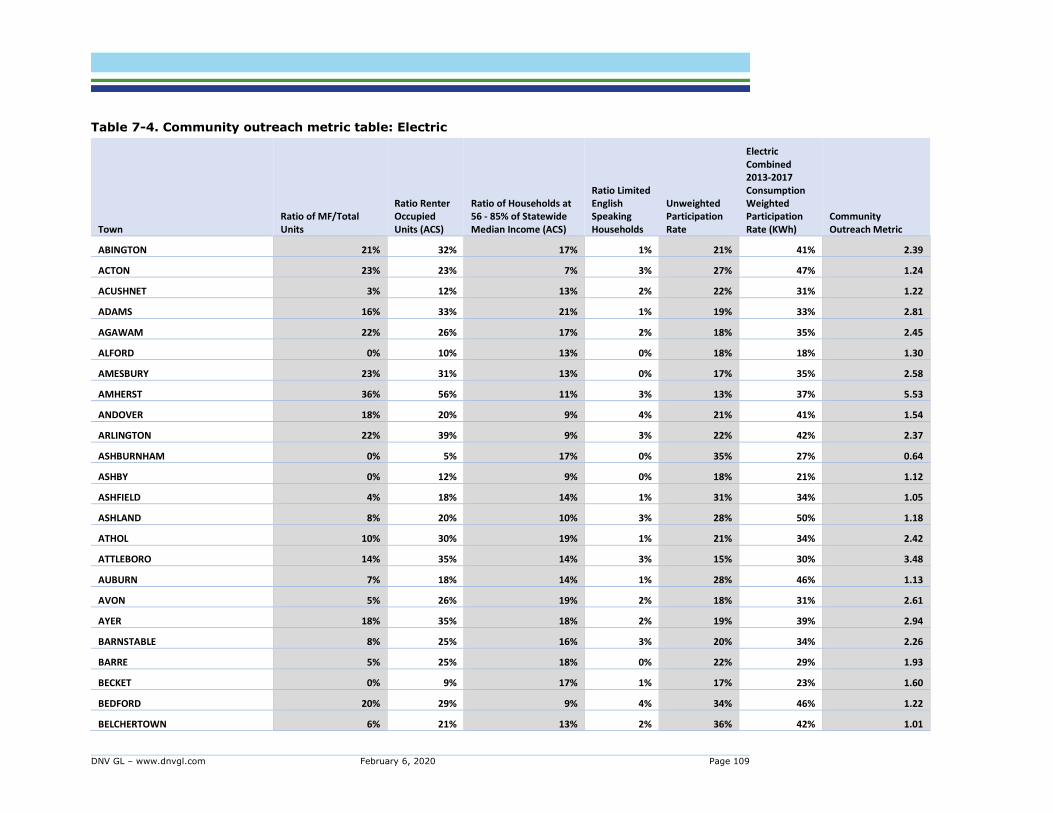
DNV GL – www.dnvgl.com February 6, 2020 Page 109
Table 7-4. Community outreach metric table: Electric
Town
Ratio of MF/Total
Units
Ratio Renter
Occupied
Units (ACS)
Ratio of Households at
56 - 85% of Statewide
Median Income (ACS)
Ratio Limited
English
Speaking
Households
Unweighted
Participation
Rate
Electric
Combined
2013-2017
Consumption
Weighted
Participation
Rate (KWh)
Community
Outreach Metric
ABINGTON 21% 32% 17% 1% 21% 41% 2.39
ACTON 23% 23% 7% 3% 27% 47% 1.24
ACUSHNET 3% 12% 13% 2% 22% 31% 1.22
ADAMS 16% 33% 21% 1% 19% 33% 2.81
AGAWAM 22% 26% 17% 2% 18% 35% 2.45
ALFORD 0% 10% 13% 0% 18% 18% 1.30
AMESBURY 23% 31% 13% 0% 17% 35% 2.58
AMHERST 36% 56% 11% 3% 13% 37% 5.53
ANDOVER 18% 20% 9% 4% 21% 41% 1.54
ARLINGTON 22% 39% 9% 3% 22% 42% 2.37
ASHBURNHAM 0% 5% 17% 0% 35% 27% 0.64
ASHBY 0% 12% 9% 0% 18% 21% 1.12
ASHFIELD 4% 18% 14% 1% 31% 34% 1.05
ASHLAND 8% 20% 10% 3% 28% 50% 1.18
ATHOL 10% 30% 19% 1% 21% 34% 2.42
ATTLEBORO 14% 35% 14% 3% 15% 30% 3.48
AUBURN 7% 18% 14% 1% 28% 46% 1.13
AVON 5% 26% 19% 2% 18% 31% 2.61
AYER 18% 35% 18% 2% 19% 39% 2.94
BARNSTABLE 8% 25% 16% 3% 20% 34% 2.26
BARRE 5% 25% 18% 0% 22% 29% 1.93
BECKET 0% 9% 17% 1% 17% 23% 1.60
BEDFORD 20% 29% 9% 4% 34% 46% 1.22
BELCHERTOWN 6% 21% 13% 2% 36% 42% 1.01

DNV GL – www.dnvgl.com February 6, 2020 Page 110
Town
Ratio of MF/Total
Units
Ratio Renter
Occupied
Units (ACS)
Ratio of Households at
56 - 85% of Statewide
Median Income (ACS)
Ratio Limited
English
Speaking
Households
Unweighted
Participation
Rate
Electric
Combined
2013-2017
Consumption
Weighted
Participation
Rate (KWh)
Community
Outreach Metric
BELLINGHAM 9% 20% 11% 3% 23% 34% 1.45
BERLIN 1% 15% 10% 0% 25% 35% 0.96
BERNARDSTON 0% 15% 18% 0% 29% 37% 1.13
BEVERLY 25% 40% 12% 1% 19% 35% 2.73
BILLERICA 14% 18% 11% 2% 24% 32% 1.30
BLACKSTONE 9% 30% 17% 1% 19% 29% 2.48
BLANDFORD 0% 6% 19% 0% 17% 19% 1.48
BOLTON 2% 6% 4% 0% 38% 44% 0.27
BOSTON 43% 65% 13% 12% 12% 39% 7.77
BOURNE 6% 23% 12% 1% 18% 32% 2.01
BOXFORD 2% 2% 8% 1% 35% 40% 0.29
BOYLSTON 0% 13% 7% 0% 12% 100% 1.71
BREWSTER 7% 16% 16% 0% 23% 40% 1.37
BRIDGEWATER 14% 25% 11% 2% 18% 35% 2.07
BRIMFIELD 1% 19% 10% 1% 24% 30% 1.26
BROCKTON 22% 46% 16% 12% 10% 27% 6.97
BROOKFIELD 3% 20% 16% 0% 22% 30% 1.62
BROOKLINE 52% 51% 8% 7% 10% 32% 6.70
BUCKLAND 3% 23% 18% 0% 26% 34% 1.54
BURLINGTON 29% 30% 12% 5% 27% 48% 1.74
CAMBRIDGE 53% 63% 11% 6% 8% 40% 9.93
CANTON 23% 22% 11% 4% 21% 42% 1.74
CARLISLE 2% 4% 3% 1% 36% 40% 0.23
CARVER 1% 7% 14% 0% 25% 45% 0.85
CHARLTON 10% 19% 11% 1% 27% 45% 1.14

DNV GL – www.dnvgl.com February 6, 2020 Page 111
Town
Ratio of MF/Total
Units
Ratio Renter
Occupied
Units (ACS)
Ratio of Households at
56 - 85% of Statewide
Median Income (ACS)
Ratio Limited
English
Speaking
Households
Unweighted
Participation
Rate
Electric
Combined
2013-2017
Consumption
Weighted
Participation
Rate (KWh)
Community
Outreach Metric
CHATHAM 3% 20% 12% 0% 16% 24% 2.06
CHELMSFORD 18% 17% 11% 2% 30% 40% 0.99
CHELSEA 40% 74% 17% 27% 11% 36% 10.34
CHESHIRE 1% 22% 25% 0% 20% 31% 2.34
CHESTER 1% 15% 12% 2% 12% 12% 2.41
CHESTERFIELD 2% 10% 18% 0% 30% 37% 0.93
CHICOPEE 0% 14% 6% 6% 9% 62% 2.82
CHILMARK 0% 20% 9% 1% 8% 12% 3.52
CLARKSBURG 3% 10% 21% 0% 24% 25% 1.30
CLINTON 21% 46% 18% 3% 16% 34% 4.30
COHASSET 8% 20% 9% 0% 27% 42% 1.09
COLRAIN 0% 21% 26% 0% 27% 31% 1.72
CONCORD 1% 6% 4% 0% 31% 67% 0.30
CONWAY 1% 11% 17% 0% 28% 34% 0.98
CUMMINGTON 2% 19% 18% 1% 17% 27% 2.26
DALTON 5% 24% 18% 1% 22% 37% 1.97
DARTMOUTH 10% 22% 14% 3% 21% 31% 1.85
DEDHAM 17% 32% 12% 2% 23% 37% 2.07
DEERFIELD 3% 26% 16% 0% 24% 33% 1.74
DENNIS 8% 21% 18% 2% 18% 33% 2.29
DIGHTON 5% 10% 13% 0% 18% 37% 1.29
DOUGLAS 10% 19% 12% 1% 24% 34% 1.28
DOVER 1% 6% 7% 0% 32% 41% 0.40
DRACUT 20% 23% 13% 1% 19% 38% 1.95
DUDLEY 9% 24% 17% 2% 20% 34% 2.16

DNV GL – www.dnvgl.com February 6, 2020 Page 112
Town
Ratio of MF/Total
Units
Ratio Renter
Occupied
Units (ACS)
Ratio of Households at
56 - 85% of Statewide
Median Income (ACS)
Ratio Limited
English
Speaking
Households
Unweighted
Participation
Rate
Electric
Combined
2013-2017
Consumption
Weighted
Participation
Rate (KWh)
Community
Outreach Metric
DUNSTABLE 0% 3% 10% 1% 29% 37% 0.45
DUXBURY 6% 11% 7% 0% 25% 39% 0.72
EAST BRIDGEWATER 7% 17% 15% 1% 21% 16% 1.57
EAST BROOKFIELD 2% 14% 11% 0% 22% 15% 1.12
EAST LONGMEADOW 9% 16% 11% 2% 25% 12% 1.16
EASTHAM 0% 15% 15% 0% 20% 29% 1.51
EASTHAMPTON 20% 44% 16% 1% 17% 41% 3.53
EASTON 11% 18% 11% 1% 22% 39% 1.41
EDGARTOWN 0% 22% 16% 3% 10% 14% 4.04
ERVING 1% 16% 18% 0% 26% 36% 1.30
ESSEX 9% 22% 15% 1% 20% 31% 1.88
EVERETT 16% 61% 20% 16% 9% 27% 10.33
FAIRHAVEN 11% 26% 13% 2% 18% 29% 2.33
FALL RIVER 30% 65% 17% 9% 6% 20% 15.07
FALMOUTH 6% 22% 13% 1% 18% 29% 1.98
FITCHBURG 17% 48% 14% 5% 6% 27% 11.96
FLORIDA 2% 11% 18% 0% 20% 23% 1.46
FOXBOROUGH 23% 34% 9% 1% 20% 33% 2.16
FRAMINGHAM 31% 46% 13% 12% 20% 42% 3.47
FRANKLIN 16% 19% 10% 1% 22% 41% 1.35
FREETOWN 0% 12% 11% 1% 27% 32% 0.90
GARDNER 26% 49% 19% 2% 14% 32% 5.03
AQUINNAH 0% 40% 9% 0% 7% 11% 6.86
GEORGETOWN 13% 20% 25% 0% 22% 70% 2.10
GILL 3% 16% 15% 2% 27% 35% 1.21
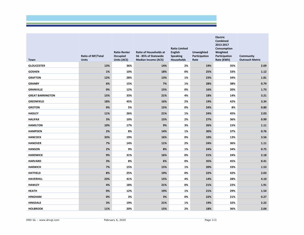
DNV GL – www.dnvgl.com February 6, 2020 Page 113
Town
Ratio of MF/Total
Units
Ratio Renter
Occupied
Units (ACS)
Ratio of Households at
56 - 85% of Statewide
Median Income (ACS)
Ratio Limited
English
Speaking
Households
Unweighted
Participation
Rate
Electric
Combined
2013-2017
Consumption
Weighted
Participation
Rate (KWh)
Community
Outreach Metric
GLOUCESTER 13% 36% 14% 2% 19% 35% 2.69
GOSHEN 1% 10% 18% 0% 25% 33% 1.12
GRAFTON 12% 28% 13% 1% 23% 34% 1.81
GRANBY 6% 15% 7% 1% 28% 38% 0.79
GRANVILLE 0% 12% 15% 0% 16% 20% 1.73
GREAT BARRINGTON 15% 33% 21% 4% 18% 14% 3.21
GREENFIELD 18% 45% 16% 2% 19% 42% 3.34
GROTON 0% 5% 15% 0% 24% 8% 0.80
HADLEY 11% 26% 21% 1% 24% 45% 2.03
HALIFAX 3% 10% 15% 2% 27% 36% 0.99
HAMILTON 10% 17% 9% 3% 26% 15% 1.11
HAMPDEN 2% 8% 14% 1% 30% 37% 0.76
HANCOCK 33% 19% 16% 0% 10% 13% 3.56
HANOVER 7% 14% 11% 2% 24% 36% 1.11
HANSON 2% 9% 8% 1% 24% 34% 0.75
HARDWICK 9% 31% 16% 0% 21% 24% 2.18
HARVARD 3% 8% 6% 0% 35% 45% 0.41
HARWICH 7% 15% 15% 1% 20% 33% 1.53
HATFIELD 8% 25% 19% 0% 22% 42% 2.03
HAVERHILL 23% 41% 15% 4% 14% 28% 4.10
HAWLEY 4% 18% 21% 0% 21% 22% 1.91
HEATH 0% 12% 19% 1% 21% 29% 1.54
HINGHAM 0% 3% 3% 0% 22% 21% 0.27
HINSDALE 3% 19% 21% 1% 19% 32% 2.22
HOLBROOK 11% 20% 15% 2% 18% 36% 2.04

DNV GL – www.dnvgl.com February 6, 2020 Page 114
Town
Ratio of MF/Total
Units
Ratio Renter
Occupied
Units (ACS)
Ratio of Households at
56 - 85% of Statewide
Median Income (ACS)
Ratio Limited
English
Speaking
Households
Unweighted
Participation
Rate
Electric
Combined
2013-2017
Consumption
Weighted
Participation
Rate (KWh)
Community
Outreach Metric
HOLLAND 0% 14% 20% 0% 18% 23% 1.94
HOLLISTON 10% 15% 9% 1% 35% 46% 0.74
HOPEDALE 5% 21% 10% 3% 28% 44% 1.23
HOPKINTON 5% 15% 7% 2% 29% 50% 0.83
HUBBARDSTON 2% 10% 16% 0% 25% 31% 1.05
HUDSON 0% 0% 13% 3% 29% 100% 0.58
HUNTINGTON 4% 15% 12% 0% 19% 26% 1.43
IPSWICH 23% 30% 16% 2% 17% 20% 2.71
KINGSTON 10% 21% 11% 0% 27% 44% 1.16
LAKEVILLE 0% 9% 9% 0% 23% 28% 0.79
LANCASTER 3% 19% 15% 3% 26% 36% 1.37
LANESBOROUGH 10% 17% 12% 0% 14% 16% 2.11
LAWRENCE 28% 72% 15% 26% 6% 28% 19.46
LEE 17% 30% 16% 3% 17% 29% 2.79
LEICESTER 12% 29% 17% 3% 25% 38% 1.94
LENOX 30% 40% 19% 2% 18% 32% 3.38
LEOMINSTER 26% 45% 14% 6% 19% 43% 3.40
LEVERETT 3% 11% 11% 0% 26% 34% 0.87
LEXINGTON 13% 19% 7% 4% 34% 47% 0.88
LEYDEN 4% 15% 16% 1% 26% 35% 1.22
LINCOLN 13% 19% 7% 2% 36% 44% 0.76
LONGMEADOW 6% 9% 9% 4% 28% 38% 0.79
LOWELL 36% 58% 16% 14% 11% 29% 8.12
LUDLOW 10% 25% 15% 7% 18% 36% 2.59
LUNENBURG 6% 20% 14% 1% 19% 34% 1.82
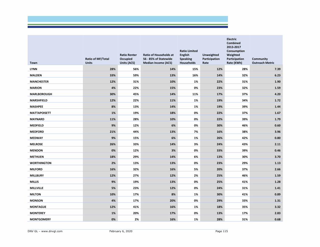
DNV GL – www.dnvgl.com February 6, 2020 Page 115
Town
Ratio of MF/Total
Units
Ratio Renter
Occupied
Units (ACS)
Ratio of Households at
56 - 85% of Statewide
Median Income (ACS)
Ratio Limited
English
Speaking
Households
Unweighted
Participation
Rate
Electric
Combined
2013-2017
Consumption
Weighted
Participation
Rate (KWh)
Community
Outreach Metric
LYNN 28% 56% 14% 15% 12% 28% 7.39
MALDEN 33% 59% 13% 16% 14% 32% 6.23
MANCHESTER 12% 31% 10% 1% 22% 31% 1.90
MARION 4% 22% 15% 0% 23% 32% 1.59
MARLBOROUGH 30% 45% 14% 11% 17% 37% 4.20
MARSHFIELD 12% 22% 11% 1% 19% 34% 1.72
MASHPEE 8% 13% 14% 1% 19% 39% 1.44
MATTAPOISETT 1% 19% 18% 0% 22% 37% 1.67
MAYNARD 11% 28% 10% 0% 22% 39% 1.79
MEDFIELD 9% 12% 6% 0% 30% 46% 0.60
MEDFORD 21% 44% 13% 7% 16% 38% 3.96
MEDWAY 9% 15% 6% 1% 26% 42% 0.80
MELROSE 26% 33% 14% 3% 24% 43% 2.11
MENDON 0% 12% 3% 0% 33% 39% 0.46
METHUEN 18% 29% 14% 6% 13% 30% 3.70
WORTHINGTON 2% 13% 13% 0% 23% 29% 1.13
MILFORD 16% 32% 16% 5% 20% 37% 2.66
MILLBURY 12% 27% 12% 2% 25% 46% 1.59
MILLIS 9% 19% 13% 0% 25% 41% 1.28
MILLVILLE 5% 23% 12% 0% 24% 31% 1.41
MILTON 10% 17% 8% 1% 30% 41% 0.89
MONSON 4% 17% 20% 0% 29% 33% 1.31
MONTAGUE 12% 41% 16% 1% 18% 35% 3.32
MONTEREY 1% 20% 17% 0% 13% 17% 2.83
MONTGOMERY 0% 2% 16% 1% 28% 31% 0.68

DNV GL – www.dnvgl.com February 6, 2020 Page 116
Town
Ratio of MF/Total
Units
Ratio Renter
Occupied
Units (ACS)
Ratio of Households at
56 - 85% of Statewide
Median Income (ACS)
Ratio Limited
English
Speaking
Households
Unweighted
Participation
Rate
Electric
Combined
2013-2017
Consumption
Weighted
Participation
Rate (KWh)
Community
Outreach Metric
MOUNT WASHINGTON 1% 15% 18% 1% 15% 9% 2.26
NAHANT 16% 32% 15% 1% 20% 26% 2.33
NANTUCKET 1% 36% 16% 3% 17% 22% 3.24
NATICK 24% 27% 13% 3% 25% 47% 1.71
NEEDHAM 12% 17% 8% 3% 29% 41% 0.94
NEW ASHFORD 4% 17% 11% 1% 13% 7% 2.26
NEW BEDFORD 20% 58% 16% 13% 8% 24% 10.77
NEW BRAINTREE 0% 11% 11% 0% 26% 29% 0.85
NEW MARLBOROUGH 0% 13% 20% 0% 14% 13% 2.36
NEW SALEM 0% 11% 17% 0% 31% 37% 0.87
NEWBURY 5% 15% 10% 1% 23% 26% 1.12
NEWBURYPORT 17% 26% 12% 0% 21% 42% 1.81
NEWTON 15% 29% 8% 5% 24% 41% 1.74
NORFOLK 2% 5% 6% 0% 39% 48% 0.28
NORTH ADAMS 18% 46% 15% 2% 17% 35% 3.74
NORTH ANDOVER 23% 27% 9% 1% 21% 40% 1.73
NORTH ATTLEBOROUGH 0% 7% 12% 0% 50% 25% 0.38
NORTH BROOKFIELD 8% 30% 18% 0% 19% 20% 2.58
NORTHAMPTON 25% 44% 13% 2% 14% 42% 4.12
NORTHBOROUGH 7% 17% 10% 1% 28% 41% 1.01
NORTHBRIDGE 14% 35% 14% 1% 18% 30% 2.69
NORTHFIELD 5% 23% 23% 0% 23% 33% 2.00
NORTON 12% 18% 11% 1% 19% 34% 1.59
NORWELL 3% 7% 10% 0% 29% 42% 0.61
OAK BLUFFS 5% 22% 16% 2% 11% 19% 3.67

DNV GL – www.dnvgl.com February 6, 2020 Page 117
Town
Ratio of MF/Total
Units
Ratio Renter
Occupied
Units (ACS)
Ratio of Households at
56 - 85% of Statewide
Median Income (ACS)
Ratio Limited
English
Speaking
Households
Unweighted
Participation
Rate
Electric
Combined
2013-2017
Consumption
Weighted
Participation
Rate (KWh)
Community
Outreach Metric
OAKHAM 0% 6% 16% 0% 24% 31% 0.90
ORANGE 16% 31% 15% 0% 21% 38% 2.25
ORLEANS 8% 23% 14% 1% 21% 35% 1.79
OTIS 1% 12% 16% 0% 10% 19% 2.69
OXFORD 12% 28% 11% 1% 24% 37% 1.64
PALMER 10% 26% 14% 0% 21% 31% 1.91
PAXTON 2% 12% 19% 0% 25% 79% 1.28
PELHAM 1% 17% 15% 1% 27% 31% 1.20
PEMBROKE 9% 13% 12% 1% 22% 34% 1.16
PEPPERELL 7% 22% 10% 0% 24% 36% 1.35
PERU 0% 8% 17% 0% 19% 22% 1.33
PETERSHAM 0% 16% 13% 0% 23% 27% 1.29
PHILLIPSTON 0% 6% 13% 1% 21% 26% 0.97
PITTSFIELD 14% 40% 16% 2% 16% 33% 3.69
PLAINFIELD 0% 11% 21% 0% 23% 27% 1.38
PLAINVILLE 15% 26% 11% 0% 14% 31% 2.74
PLYMOUTH 9% 22% 15% 2% 22% 39% 1.72
PLYMPTON 4% 13% 11% 0% 30% 40% 0.79
PROVINCETOWN 21% 33% 14% 2% 13% 40% 3.74
QUINCY 35% 53% 14% 12% 15% 38% 5.44
RANDOLPH 21% 31% 16% 8% 17% 35% 3.25
READING 25% 30% 8% 0% 22% 82% 1.77
REHOBOTH 0% 9% 11% 2% 26% 32% 0.81
REVERE 25% 52% 18% 13% 13% 33% 6.62
RICHMOND 2% 10% 14% 0% 20% 26% 1.18

DNV GL – www.dnvgl.com February 6, 2020 Page 118
Town
Ratio of MF/Total
Units
Ratio Renter
Occupied
Units (ACS)
Ratio of Households at
56 - 85% of Statewide
Median Income (ACS)
Ratio Limited
English
Speaking
Households
Unweighted
Participation
Rate
Electric
Combined
2013-2017
Consumption
Weighted
Participation
Rate (KWh)
Community
Outreach Metric
ROCHESTER 0% 10% 13% 1% 32% 36% 0.76
ROCKLAND 19% 28% 15% 1% 21% 41% 2.10
ROCKPORT 8% 31% 17% 0% 21% 35% 2.22
ROWE 2% 22% 19% 0% 20% 28% 2.04
ROYALSTON 0% 17% 24% 0% 17% 16% 2.47
RUSSELL 1% 10% 21% 0% 18% 28% 1.68
RUTLAND 4% 13% 12% 0% 24% 36% 1.06
SALEM 29% 52% 14% 5% 15% 44% 4.64
SALISBURY 8% 25% 15% 0% 15% 29% 2.59
SANDISFIELD 0% 8% 23% 1% 14% 18% 2.27
SANDWICH 3% 15% 14% 0% 23% 36% 1.23
SAUGUS 14% 21% 12% 2% 20% 36% 1.80
SAVOY 1% 11% 17% 0% 23% 27% 1.22
SCITUATE 5% 14% 7% 0% 21% 38% 1.03
SEEKONK 1% 13% 13% 1% 22% 31% 1.28
SHARON 8% 14% 8% 4% 29% 43% 0.87
SHEFFIELD 3% 19% 15% 0% 17% 21% 1.98
SHELBURNE 11% 36% 19% 1% 22% 31% 2.54
SHERBORN 4% 7% 5% 1% 36% 45% 0.36
SHIRLEY 8% 30% 15% 0% 21% 45% 2.16
SHREWSBURY 18% 14% 8% 5% 11% 52% 2.44
SHUTESBURY 2% 11% 11% 0% 25% 34% 0.86
SOMERSET 3% 19% 13% 3% 15% 25% 2.37
SOMERVILLE 26% 65% 14% 8% 9% 29% 9.69
SOUTHAMPTON 5% 10% 18% 1% 23% 30% 1.27

DNV GL – www.dnvgl.com February 6, 2020 Page 119
Town
Ratio of MF/Total
Units
Ratio Renter
Occupied
Units (ACS)
Ratio of Households at
56 - 85% of Statewide
Median Income (ACS)
Ratio Limited
English
Speaking
Households
Unweighted
Participation
Rate
Electric
Combined
2013-2017
Consumption
Weighted
Participation
Rate (KWh)
Community
Outreach Metric
SOUTHBOROUGH 1% 11% 7% 1% 31% 43% 0.61
SOUTHBRIDGE 17% 57% 18% 10% 12% 31% 6.96
SOUTHWICK 9% 19% 13% 0% 21% 29% 1.50
SPENCER 12% 36% 12% 1% 17% 37% 2.89
SPRINGFIELD 21% 53% 16% 12% 11% 30% 7.38
STOCKBRIDGE 11% 32% 18% 0% 16% 22% 3.16
STONEHAM 30% 36% 14% 3% 23% 45% 2.30
STOUGHTON 18% 28% 13% 5% 16% 34% 2.85
STOW 14% 16% 5% 0% 25% 54% 0.82
STURBRIDGE 12% 18% 14% 3% 26% 41% 1.35
SUDBURY 4% 9% 6% 1% 40% 49% 0.39
SUNDERLAND 36% 57% 14% 3% 23% 48% 3.13
SUTTON 3% 9% 10% 0% 32% 42% 0.61
SWAMPSCOTT 14% 23% 8% 3% 26% 41% 1.30
SWANSEA 2% 13% 14% 3% 17% 27% 1.72
TEMPLETON 5% 10% 19% 0% 50% 38% 0.57
TEWKSBURY 12% 14% 10% 1% 22% 41% 1.13
TISBURY 2% 32% 18% 5% 14% 20% 4.00
TOLLAND 0% 15% 12% 0% 13% 13% 2.01
TOPSFIELD 2% 8% 10% 0% 31% 44% 0.60
TOWNSEND 9% 20% 13% 0% 14% 23% 2.35
TRURO 4% 17% 10% 0% 18% 26% 1.54
TYNGSBOROUGH 10% 14% 13% 2% 25% 35% 1.12
TYRINGHAM 1% 9% 8% 1% 14% 14% 1.29
UPTON 5% 18% 6% 1% 28% 40% 0.84

DNV GL – www.dnvgl.com February 6, 2020 Page 120
Town
Ratio of MF/Total
Units
Ratio Renter
Occupied
Units (ACS)
Ratio of Households at
56 - 85% of Statewide
Median Income (ACS)
Ratio Limited
English
Speaking
Households
Unweighted
Participation
Rate
Electric
Combined
2013-2017
Consumption
Weighted
Participation
Rate (KWh)
Community
Outreach Metric
UXBRIDGE 5% 21% 12% 1% 24% 40% 1.46
WAKEFIELD 0% 8% 10% 3% 11% 17% 1.81
WALES 2% 20% 16% 2% 17% 21% 2.17
WALPOLE 11% 18% 11% 1% 23% 40% 1.29
WALTHAM 30% 50% 13% 6% 14% 35% 5.09
WARE 10% 29% 20% 1% 21% 34% 2.34
WAREHAM 6% 23% 15% 1% 17% 35% 2.29
WARREN 10% 30% 17% 0% 16% 23% 2.92
WARWICK 1% 10% 14% 0% 25% 30% 0.96
WASHINGTON 0% 1% 15% 0% 15% 21% 1.07
WATERTOWN 24% 49% 12% 4% 15% 41% 4.29
WAYLAND 6% 12% 4% 2% 34% 44% 0.53
WEBSTER 15% 46% 18% 4% 14% 31% 4.85
WELLFLEET 1% 16% 18% 0% 19% 29% 1.79
WENDELL 0% 14% 17% 2% 37% 33% 0.92
WENHAM 10% 12% 13% 0% 28% 37% 0.91
WEST BRIDGEWATER 3% 14% 16% 0% 21% 19% 1.40
WEST BROOKFIELD 13% 29% 15% 0% 20% 20% 2.17
WEST NEWBURY 1% 5% 7% 0% 32% 39% 0.36
WEST SPRINGFIELD 23% 40% 18% 5% 15% 33% 4.14
WEST STOCKBRIDGE 1% 10% 16% 0% 18% 12% 1.43
WEST TISBURY 0% 15% 10% 0% 14% 19% 1.76
WESTBOROUGH 33% 39% 8% 3% 21% 49% 2.39
WESTFIELD 8% 10% 10% 2% 33% 10% 0.65
WESTFORD 5% 11% 9% 2% 29% 41% 0.74

DNV GL – www.dnvgl.com February 6, 2020 Page 121
Town
Ratio of MF/Total
Units
Ratio Renter
Occupied
Units (ACS)
Ratio of Households at
56 - 85% of Statewide
Median Income (ACS)
Ratio Limited
English
Speaking
Households
Unweighted
Participation
Rate
Electric
Combined
2013-2017
Consumption
Weighted
Participation
Rate (KWh)
Community
Outreach Metric
WESTHAMPTON 0% 9% 13% 0% 29% 33% 0.76
WESTMINSTER 7% 13% 5% 0% 23% 35% 0.81
WESTON 7% 15% 5% 3% 30% 32% 0.78
WESTPORT 4% 16% 10% 2% 16% 24% 1.75
WESTWOOD 17% 13% 9% 2% 28% 44% 0.85
WEYMOUTH 30% 36% 15% 2% 21% 38% 2.52
WHATELY 0% 15% 19% 2% 26% 31% 1.37
WHITMAN 12% 28% 14% 0% 21% 36% 1.99
WILBRAHAM 4% 11% 8% 1% 29% 41% 0.68
WILLIAMSBURG 5% 22% 11% 0% 27% 36% 1.21
WILLIAMSTOWN 11% 27% 16% 2% 19% 30% 2.37
WINCHENDON 9% 22% 16% 1% 15% 24% 2.57
WINCHESTER 11% 15% 8% 3% 31% 43% 0.81
WINDSOR 0% 1% 15% 0% 19% 22% 0.84
WINTHROP 21% 43% 15% 4% 15% 38% 4.15
WOBURN 24% 38% 14% 4% 23% 41% 2.44
WORCESTER 27% 57% 16% 11% 12% 32% 7.30
WRENTHAM 5% 16% 9% 0% 25% 37% 1.00
YARMOUTH 11% 21% 21% 3% 20% 36% 2.26
Grand Total 21% 39% 13% 6% 16% 35% 3.57
DNV GL – www.dnvgl.com February 6, 2020 Page 122
8 APPENDIX C: BIVARIATE MAPS
DNV GL originally provided the bivariate maps to the PAs in a powerpoint file. The slides of that file are
reproduced as images in this appendix.
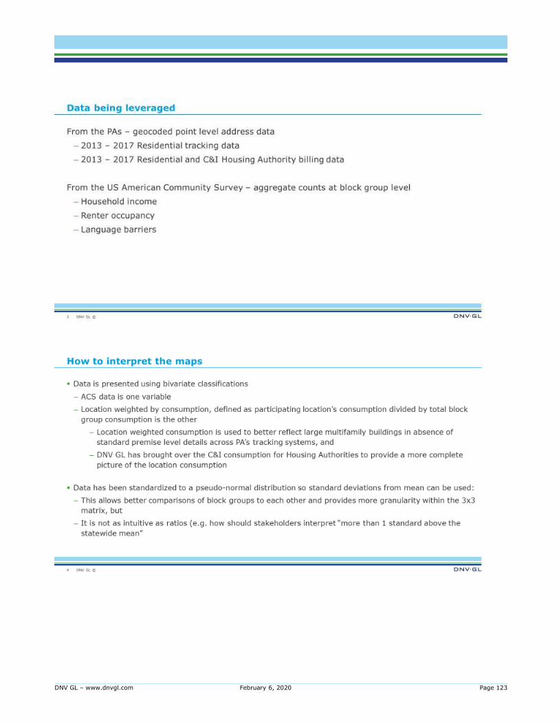
DNV GL – www.dnvgl.com February 6, 2020 Page 123

DNV GL – www.dnvgl.com February 6, 2020 Page 124

DNV GL – www.dnvgl.com February 6, 2020 Page 125
Combined gas and electric consumption weighted participation * Renter-occupied households

DNV GL – www.dnvgl.com February 6, 2020 Page 126
Combined gas and electric consumption weighted participation * Limited-English households

DNV GL – www.dnvgl.com February 6, 2020 Page 127
Combined gas and electric consumption weighted participation * Moderate income (40k-60k)
households

DNV GL – www.dnvgl.com February 6, 2020 Page 128
Electric consumption weighted participation * Renter-occupied households

DNV GL – www.dnvgl.com February 6, 2020 Page 129
Electric consumption weighted participation * Limited-English households

DNV GL – www.dnvgl.com February 6, 2020 Page 130
Electric consumption weighted participation * Moderate income (40k-60k) households

DNV GL – www.dnvgl.com February 6, 2020 Page 131
Gas consumption weighted participation * Renter-occupied households

DNV GL – www.dnvgl.com February 6, 2020 Page 132
Gas consumption weighted participation * Limited-English households
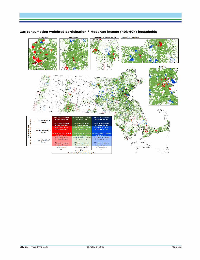
DNV GL – www.dnvgl.com February 6, 2020 Page 133
Gas consumption weighted participation * Moderate income (40k-60k) households

DNV GL – www.dnvgl.com February 6, 2020 Page 134

DNV GL – www.dnvgl.com February 6, 2020 Page 135
9 APPENDIX D: CLOSE-UP HOTSPOT MAPS
The close-up hot spot maps provide the same information as the statewide hotspot map, but covering
smaller areas. DNV GL generated a composite number for each block group and then input these composite
numbers to generate a geographic hot spot map based on areas where there are concentrations of
consistently high (or low) block group scores.35 We defined an area as the block groups adjacent to a given
block group. 36 The composite number is calculated by taking the sum of the ratios of the following
attributes:
1. Percentage of households that are moderate income37
2. Percentage of households that are renter-occupied
3. Percentage of households with a primary language other than English
4. Percentage of households that are in structures of 5 or more units (i.e., a proxy for multifamily)
5. Percentage of structures that were built prior to 1940
The hot spot maps do not factor in participation status.
35 For technical details on ESRI’s implementation of hot spot analysis and additional context, please see https://pro.arcgis.com/en/pro-app/tool-
reference/spatial-statistics/h-how-hot-spot-analysis-getis-ord-gi-spatial-stati.htm. 36 We chose to look at adjacent block group areas in consideration of differences in block group area between densely populated cities like Boston and
rural towns like Mt. Washington, and of our understanding that stakeholders are more interested in local geographic differences than large scale regional differences. Other representations we considered were a Euclidean distance function (e.g., look at all block groups within 5 miles) and
an inverse distance weight (e.g., look at all block groups within 5 miles, but as we get further away, assign a lower hot spot impact weight to
the block groups). In both cases, DNV GL felt that the regional scale differences between the rural western and central parts of the state versus
the densely populated eastern part of the state precluded using distance as our weighting variable. 37 As defined earlier in this report
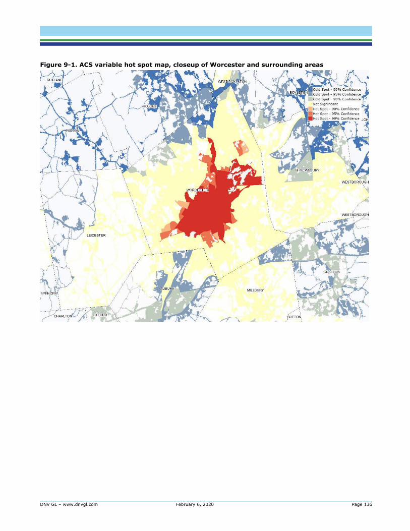
DNV GL – www.dnvgl.com February 6, 2020 Page 136
Figure 9-1. ACS variable hot spot map, closeup of Worcester and surrounding areas

DNV GL – www.dnvgl.com February 6, 2020 Page 137
Figure 9-2. ACS variable hot spot map, closeup of Springfield, Holyoke, and surrounding areas

DNV GL – www.dnvgl.com February 6, 2020 Page 138
Figure 9-3. ACS variable hot spot map, closeup of Lawrence and surrounding areas

DNV GL – www.dnvgl.com February 6, 2020 Page 139
Figure 9-4. ACS variable hot spot map, closeup of Fitchburg and surrounding areas

DNV GL – www.dnvgl.com February 6, 2020 Page 140
Figure 9-5. ACS variable hot spot map, closeup of Fall River and surrounding areas

DNV GL – www.dnvgl.com February 6, 2020 Page 141
Figure 9-6. ACS variable hot spot map, closeup of Boston and surrounding areas

ABOUT DNV GL Driven by our purpose of safeguarding life, property and the environment, DNV GL enables organizations to advance the safety and sustainability of their business. We provide classification and technical assurance along with software and independent expert advisory services to the maritime, oil and gas, and energy industries. We also provide certification services to customers across a wide range of industries. Operating in more than 100 countries, our 16,000 professionals are dedicated to helping our customers make the world safer, smarter, and greener.