Embed Size (px)
Citation preview
SOUTH COAST AIR QUALITY MANAGEMENT DISTRICT
Sample Construction Scenarios for Projects Less than Five Acres in Size
February 2005
Executive Officer Barry R. Wallerstein, D. Env.
Deputy Executive Officer Planning, Rule Development, and Area Sources Elaine Chang, DrPH
Assistant Deputy Executive Officer Planning, Rule Development, and Area Sources Laki Tisopulos, Ph.D., P.E.
Planning and Rules Manager Susan Nakamura Author: James Koizumi, Air Quality Specialist Reviewed By: Steve Smith, Ph.D. – Program Supervisor Jeri Vogue - Senior Deputy District Counsel Technical Assistance: Barbara A. Radlein, Air Quality Specialist

SOUTH COAST AIR QUALITY MANAGEMENT DISTRICT GOVERNING BOARD
CHAIRMAN: WILLIAM A. BURKE, Ed.D. Speaker of the Assembly Appointee VICE CHAIRMAN: S. ROY WILSON, Ed.D. Supervisor, Fourth District Riverside County Representative MEMBERS: MICHAEL D. ANTONOVICH Supervisor, Fifth District Los Angeles County Representative JANE W. CARNEY Senate Rules Committee Appointee BEATRICE J.S. LAPISTO-KIRTLEY Mayor, City of Bradbury Cities Representative, Los Angeles County, Eastern Region RONALD O. LOVERIDGE Mayor, City of Riverside Cities Representative, Riverside County JAN PERRY Councilmember, Ninth District Cities Representative, Los Angeles County, Western Region MIGUEL A. PULIDO Mayor, City of Santa Ana Cities Representative, Orange County GARY OVITT Supervisor, Fourth District San Bernardino County Representative JAMES SILVA
Supervisor, Second District Orange County Representative CYNTHIA VERDUGO-PERALTA Governor's Appointee DENNIS YATES Mayor, City of Chino Cities Representative, San Bernardino County EXECUTIVE OFFICER: BARRY R. WALLERSTEIN, D.Env.
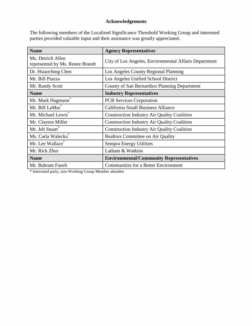
Acknowledgements The following members of the Localized Significance Threshold Working Group and interested parties provided valuable input and their assistance was greatly appreciated. Name Agency Representatives
Ms. Detrich Allen represented by Ms. Renee Brandt
City of Los Angeles, Environmental Affairs Department
Dr. Hsiaoching Chen Los Angeles County Regional Planning
Mr. Bill Piazza Los Angeles Unified School District
Mr. Randy Scott County of San Bernardino Planning Department
Name Industry Representatives Mr. Mark Hagmann* PCR Services Corporation
Mr. Bill LaMar* California Small Business Alliance
Mr. Michael Lewis* Construction Industry Air Quality Coalition
Mr. Clayton Miller Construction Industry Air Quality Coalition
Mr. Jeb Stuart* Construction Industry Air Quality Coalition
Ms. Carla Walecka* Realtors Committee on Air Quality
Mr. Lee Wallace* Sempra Energy Utilities
Mr. Rick Zbur Latham & Watkins
Name Environmental/Community Representatives Mr. Bahram Fazeli Communities for a Better Environment * Interested party, non-Working Group Member attendee
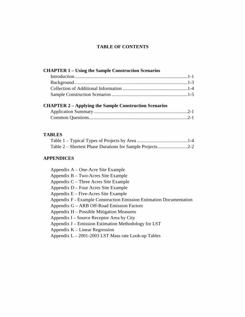
TABLE OF CONTENTS
CHAPTER 1 – Using the Sample Construction Scenarios Introduction..............................................................................................1-1 Background..............................................................................................1-3 Collection of Additional Information ......................................................1-4 Sample Construction Scenarios ...............................................................1-5
CHAPTER 2 – Applying the Sample Construction Scenarios
Application Summary ..............................................................................2-1 Common Questions..................................................................................2-1
TABLES
Table 1 – Typical Types of Projects by Area ..........................................1-4 Table 2 – Shortest Phase Durations for Sample Projects.........................2-2
APPENDICES
Appendix A – One-Acre Site Example Appendix B – Two-Acres Site Example Appendix C – Three Acres Site Example Appendix D – Four Acres Site Example Appendix E – Five-Acres Site Example Appendix F - Example Construction Emission Estimation Documentation Appendix G – ARB Off-Road Emission Factors Appendix H – Possible Mitigation Measures Appendix I – Source Receptor Area by City Appendix J – Emission Estimation Methodology for LST Appendix K – Linear Regression Appendix L – 2001-2003 LST Mass rate Look-up Tables
February 2005
C H A P T E R 1 U S I N G T H E S A M P L E C O N S T R U C T I O N S C E N A R I O S
Introduction
Background
Collection of Additional Information
Sample Construction Scenarios
Chapter 1 – Using the Sample Construction Scenarios Sample Construction Scenarios
1-1 February 2005
INTRODUCTION In accordance with South Coast Air Quality Management District (SCAQMD) Governing Board’s direction, staff has developed the localized significance threshold (LST) methodology and mass rate look-up tables, which were formally adopted by the Governing Board on October 3, 2003 for voluntary use by other public agencies. The mass rate LST look-up tables are only applicable to the following criteria pollutants: oxides of nitrogen (NOX), carbon monoxide (CO), and particulate matter less than 10 microns in aerodynamic diameter (PM10). The mass rate look-up tables were developed for each source receptor area (SRA) and can be used on a voluntary basis by public agencies to determine whether or not a project may generate significant adverse localized air quality impacts. LSTs represent the maximum emissions from a project that are not expected to cause or contribute to an exceedance of the most stringent applicable federal or state ambient air quality standards, and are developed based on the ambient concentrations of that pollutant for each source receptor area. For PM10 LSTs, mass rate look-up tables were derived based on requirements in SCAQMD Rule 403 – Fugitive Dust. Intended Use of LSTs by Local Public Agencies The use of LSTs is voluntary, to be implemented at the discretion of local public agencies acting as a lead agencies pursuant to the California Environmental Quality Act (CEQA) or the National Environmental Policy Act (NEPA). Detailed information on the methodology used to derive the mass rate LST look-up tables can be viewed at the following SCAQMD website address: http://www.aqmd.gov/hb/031034a.html. LSTs Applicability LSTs would only apply to projects that must undergo an environmental analysis pursuant to CEQA or the National Environmental Policy Act (NEPA). Projects that are statutorily or categorically exempt under CEQA would not be subject to LST analyses. Projects exempt from CEQA also include infill projects that meet the H&S Code provisions or projects identified by lead agencies as ministerial. The methodology and screening tables have been prepared to be included as an appendix to the SCAQMD CEQA Air Quality Handbook (Handbook). Mass rate LST Look-Up Tables Applicability The mass rate LST look-up tables apply only to projects that are less than or equal to five acres. Lead agencies may use the mass rate LST look-up tables to determine localized air quality impacts or use the LST mass look-up tables as a screening tool. If the project exceeds any applicable LST when the mass rate look-up tables are used in a screening analysis, then project specific air quality modeling may be performed. In the event that the project area exceeds five acres, it is recommended that lead agencies perform project-specific air quality modeling for these larger projects. PM10 LSTs were derived based on concentration requirements in Rule 403 – Fugitive Dust, and tend to be more limiting than the CO or NOx LSTs. The Handbook, however, identifies a substantial number of PM10 (fugitive dust) mitigation measures that may be used to mitigate project PM10 emissions to less than the relevant PM10 mass rate LST. In general, LSTs are derived based on the location of the activity (i.e., the SRA); the project emission rates of NOX, CO, and PM10; and the distance to the nearest exposed individual. The location of the activity and the distance to the nearest exposed individual can be determined by maps, aerial and site
Chapter 1 – Using the Sample Construction Scenarios Sample Construction Scenarios
1-2 February 2005
photos, or site visits. To calculate NOx, CO, and PM10 emissions, the methodologies, emission factors and/or rates identified in the Handbook may be used (see Chapter 9 and the Appendix to Chapter 9). Relative to construction, the lead agency may use the sample construction scenarios described in the following sections. If lead agencies use the mass rate LST look-up tables and determine that the proposed project under consideration exceeds any applicable LST, they may choose to apply any of the substantial number of applicable mitigation measures identified in Chapter 11 of the Handbook to the proposed projects (see Appendix H). Format and Use of This Document This document is intended to provide local lead agencies with the information necessary to perform a localized air quality analysis. The format of this document consists of the following. Chapter 1 • Introduction • Background - contains information on the development of the LSTs. • The Pilot Study - describes the pilot study that was conducted to develop more accurate
sample construction scenarios. The actual sample construction scenarios can be found in Appendices A through E.
• Sample Construction Scenarios - explains the three ways that the construction scenarios can be use by lead agencies, which include using the sample construction scenarios to represent the proposed project, using the sample construction scenario spreadsheets as a template or basis to prepare project-specific analyses, or using a combination of those approaches for various proposed project phases.
Chapter 2 • Applying the Sample Construction Scenarios - this chapter provides guidance for applying
the sample construction scenarios to specific projects when the projects do not conform exactly to the characteristics of the applicable sample construction scenario.
Appendices • Appendices A through E - contain each individual sample construction scenario, one through
five acres, respectively. • Appendix F - provides the sources of emission factors and emission calculation
methodologies. • Appendix G - provides simplified off-road emission factors to assist planners with
calculating construction equipment emissions. • Appendix H - contains a list of mitigation measures and control efficiencies from the
SCAQMD’s CEQA Air Quality Handbook to assist planners with identifying measures to mitigate impacts from a project.
• Appendix I - contains a table that allows planners to identify the source receptor area of their proposed project from the city where the proposed project would be located. The source receptor area is used to identify which LST from the mass rate LST look-up tables is applicable to the proposed project.
• Appendix J - details how to scale mass rate LSTs for proposed projects with plot sizes that are in between the plot sizes in the mass rate LST look-up tables.
Chapter 1 – Using the Sample Construction Scenarios Sample Construction Scenarios
1-3 February 2005
• Appendix K - contains the mass rate look-up tables for proposed project site between one and five acres for each source receptor area.
BACKGROUND The LST methodology is applicable to projects where emission sources occupy a fixed location. This means that the LST methodology will apply to projects during construction because, although construction equipment may move around the construction site, their movements are restricted to a fixed location. The LST methodology would typically not apply to the operational phase of project because emissions are primarily generated by mobile sources traveling on local roadways over potentially large distances or areas. LSTs would apply to the operational phase of a project, if the project includes stationary sources or attracts mobile sources that may spend long periods queuing and idling at the site. For example, the LST methodology could apply to projects such as warehouse/transfer facilities. During development of the LST methodology and mass rate look-up tables, SCAQMD staff received comments stating that using the LSTs may require a more detailed analysis of air quality impacts than are currently prepared. As a result, local planners requested guidance on setting up construction scenarios and assistance with calculating construction air quality impacts in addition to using the methodologies in the Handbook. In response to this request, in October 2003 SCAQMD staff developed three sample construction scenarios, one-acre, two-acre, and five-acre in size, where construction impacts do not exceed the most stringent LSTs. The sample scenarios were designed to be used by local lead agencies as models or templates for analyzing construction air quality impacts for projects undergoing an environmental analysis under CEQA or the National Environmental Policy Act NEPA. At the October 3, 2003 Governing Board Hearing, SCAQMD staff presented the LST methodology, mass rate look-up tables, and the sample construction scenarios to the Governing Board for consideration. The Governing Board adopted the LST methodology1 pursuant to CEQA Guidelines Section 15064.7. However, in the adopting resolution, the Governing Board directed staff to conduct a nine-month phase-in period for field testing. The objective of the field testing was to conduct a pilot program with cities and local contractors to assess any potential implementation issues and report to the SCAQMD’s Mobile Source Committee, at which time the Mobile Source Committee would formally approve complete implementation of the LST methodology or provide further direction. Staff was also asked to expand the list of sample construction scenarios to reduce resource impacts to local government and contractors by streamlining the construction analysis, updating mitigation measures with notations as to the appropriateness of specific measures for projects of different sizes, and reconvening the working group to review the results of the field testing and evaluate refinements or improvements needed to further simplify use of the LST methodology for local lead agencies.
1 It should be noted that the action taken by the Governing Board was to adopt the LST methodology. The reason for adopting the methodology rather than the mass rate look-up tables is that the mass rate look-up tables for CO and NOx are based on ambient concentrations. Because monitored ambient concentrations change from year to year, the mass rate look-up tables must be modified annually to reflect the most recent three years of monitored data. This approach allows staff to update the mass rate emission tables without approval from the Governing Board. Governing Board approval is required if the LST methodology is modified.
Chapter 1 – Using the Sample Construction Scenarios Sample Construction Scenarios
1-4 February 2005
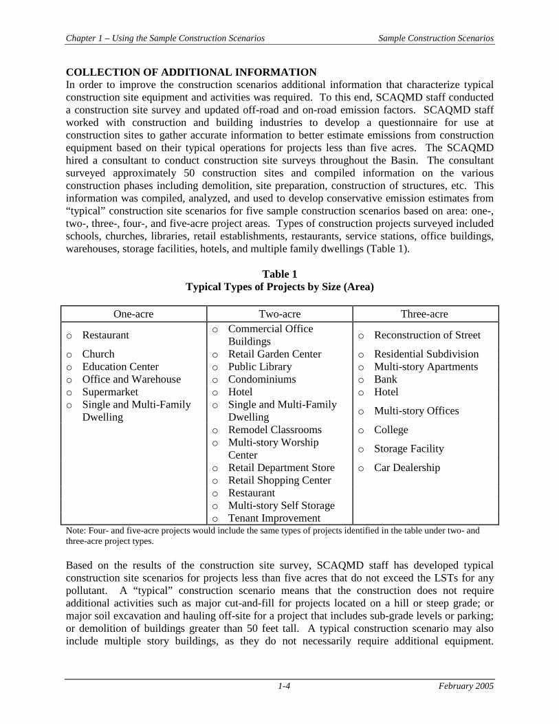
COLLECTION OF ADDITIONAL INFORMATION In order to improve the construction scenarios additional information that characterize typical construction site equipment and activities was required. To this end, SCAQMD staff conducted a construction site survey and updated off-road and on-road emission factors. SCAQMD staff worked with construction and building industries to develop a questionnaire for use at construction sites to gather accurate information to better estimate emissions from construction equipment based on their typical operations for projects less than five acres. The SCAQMD hired a consultant to conduct construction site surveys throughout the Basin. The consultant surveyed approximately 50 construction sites and compiled information on the various construction phases including demolition, site preparation, construction of structures, etc. This information was compiled, analyzed, and used to develop conservative emission estimates from “typical” construction site scenarios for five sample construction scenarios based on area: one-, two-, three-, four-, and five-acre project areas. Types of construction projects surveyed included schools, churches, libraries, retail establishments, restaurants, service stations, office buildings, warehouses, storage facilities, hotels, and multiple family dwellings (Table 1).
Table 1 Typical Types of Projects by Size (Area)
One-acre Two-acre Three-acre
o Restaurant o Commercial Office
Buildings o Reconstruction of Street
o Church o Retail Garden Center o Residential Subdivision o Education Center o Public Library o Multi-story Apartments o Office and Warehouse o Condominiums o Bank o Supermarket o Hotel o Hotel o Single and Multi-Family
Dwelling o Single and Multi-Family
Dwelling o Multi-story Offices
o Remodel Classrooms o College
o Multi-story Worship
Center o Storage Facility
o Retail Department Store o Car Dealership o Retail Shopping Center o Restaurant o Multi-story Self Storage o Tenant Improvement
Note: Four- and five-acre projects would include the same types of projects identified in the table under two- and three-acre project types. Based on the results of the construction site survey, SCAQMD staff has developed typical construction site scenarios for projects less than five acres that do not exceed the LSTs for any pollutant. A “typical” construction scenario means that the construction does not require additional activities such as major cut-and-fill for projects located on a hill or steep grade; or major soil excavation and hauling off-site for a project that includes sub-grade levels or parking; or demolition of buildings greater than 50 feet tall. A typical construction scenario may also include multiple story buildings, as they do not necessarily require additional equipment.
Chapter 1 – Using the Sample Construction Scenarios Sample Construction Scenarios
1-5 February 2005
Multiple story buildings may simply require additional time (days) to complete construction. Lead agencies with proposed projects that involve construction of a multi-storied building can use the sample construction scenarios to directly represent the proposed project as long as the amounts and types of the construction equipment are consistent with those in the sample construction scenarios. Aside from these restrictions, the sample construction scenarios can be applied to any type of construction project, commercial, residential, educational, etc. (Table 1). Additional technical enhancements were made to update off-road and on-road emission factors based on ARB’s Off-Road and EMFAC2002 models that will simplify emission calculations from off-road and on-road2 equipment. Future Enhancements Staff welcomes input and feedback from interested parties for improving the accuracy of the construction scenarios. Staff will also consider developing additional construction scenarios that may be generally applicable to a range of different land use projects. SCAQMD staff is available to assist lead agencies or project proponents in addressing implementation issues. For those parties interested in information on the methodology for deriving the LSTs, the reader is referred to the following document Draft Localized Significance Threshold Methodology. For additional information on analyzing air quality impacts in general, the reader is referred to the following available sources: Handbook, U.S. EPA’s AP-42, or to California Air Resources Board’s URBEMIS2002 model at the following internet address: http://www.arb.ca.gov/planning/urbemis/urbemis.htm. SAMPLE CONSTRUCTION SCENARIOS SCAQMD staff has prepared sample construction scenarios that generically represent a broad range of project types that occur in the district, e.g., commercial, residential, educational, etc., (Table 1). Each sample construction scenario is divided into five non-overlapping phases: demolition, site preparation, grading, building, and architectural coatings and paving. Based on actual construction equipment and activity (hours of operation, area disturbed, dirt and debris handled, etc.) obtained from the construction site surveys, the sample construction scenarios in Appendices A through E represent projects that do not exceed the most stringent localized significance thresholds identified in the mass emission look-up tables. The sample construction scenarios spreadsheets can be downloaded from the SCAQMD’s website at http://www.aqmd.gov/ceqa/hdbk.html. The most stringent localized significance thresholds represent the lowest allowable mass emissions for a pollutant from any SRA. In practice, if the lead agency calculates mass emissions from a proposed project, the resulting emissions should be compared to the appropriate mass rate look-up table based on the proposed project location (SRA), project size (area), and distance to the sensitive receptor. For lead agencies that do not perform project-specific calculations or modeling to analyze localized air quality impacts, sample construction scenarios can be used based on the needs and/or air quality analysis expertise of the local lead agencies. The local lead agencies can use the sample construction scenarios to varying degrees including relying completely on the
2 Emissions for a localized impact analysis would include only those emissions that occur on-site, such as watering truck travel, or haul/delivery truck travel through the site. Emissions from on-road vehicles off-site would not be included in a localized impact analysis; however, these emissions should be included in the regional impact analysis.
Chapter 1 – Using the Sample Construction Scenarios Sample Construction Scenarios
1-6 February 2005
relevant sample construction scenario to represent the proposed project to selecting a sample construction scenario as a starting point for the air quality analysis and then modifying the equations or assumptions to fit site-specific characteristics of the project undergoing the environmental analysis. The following subsections describe the ways in which the sample construction scenarios might be used by local lead agencies. 1. Sample Construction Scenario Representative of Proposed Project – No
Modification If a proposed project is five acres or less and does not require additional construction activities such as major cut-and-fill, or excavation for sub-grade levels or parking, or demolition of a structure taller than 50 feet, the lead agency can use the applicable sample construction scenario to represent the emissions and impacts from the propose project instead of preparing a project-specific construction air quality analysis. No additional quantification of construction emissions would be necessary. Using the sample construction scenario to represent the emissions and impacts from the propose project would allow the lead agency to conclude that localized air quality impacts during construction do not exceed any applicable LSTs in the mass rate tables. Like any other condition proposed in air quality analysis, if a lead agency decides to use a sample construction scenario to represent a proposed project, the lead agency would be required to ensure that actual project construction parameters generally are similar to, or less than, the construction parameters described in the sample project. Construction parameters include number of pieces and size of construction equipment, operating hours, area disturbed, dirt or debris handled, etc. To ensure that the sample construction scenarios are implemented, the lead agency could require the project proponent to adhere to the construction scenario as either part of the project description that is approved by the decision makers or as mitigation in an approved mitigation monitoring plan. 2. Sample Construction Scenario as a Basis for Estimating Emissions with Project
Specific Information – Use of Scenarios as a template In this situation, the lead agency wishes to establish project-specific construction scenarios for each construction phase. The lead agency would use the sample scenarios as templates or a basis to estimate project-specific emissions and analysis. The lead agency would calculate project-specific construction air quality impacts by using the same methodologies used to derive the sample construction scenarios, but tailoring them to fit the project-specific characteristics for the project under consideration. Lead agencies can download the spreadsheets used to derive the sample projects from the SCAQMD’s website at http://www.aqmd.gov/ceqa/hdbk.html, and then use the spreadsheets to develop scenarios that fit their proposed project by changing the types, dimensions and numbers of equipment, workers, operation schedules, areas disturbed, dirt and debris handled, and trips described in the sample scenarios. Spreadsheet options that can be changed include the following:
• The number, rating, or load of equipment • The number of workers • The daily hours of use for equipment or operations • The amounts of materials handled • The size of the areas disturbed • The dimensions of the structures demolished or built • The mitigation measures or control efficiencies
Chapter 1 – Using the Sample Construction Scenarios Sample Construction Scenarios
1-7 February 2005
• The lengths or number of trips • The types of operations • The emission equations or parameters used in the equations • LSTs from project specific source receptor areas. Use the city of proposed project
and the table in Appendix I to find the source receptor area of the proposed project, and then use the LST mass rate look-up tables to find the corresponding LSTs.
The shaded cells in the sample construction scenario spreadsheets are typical values that lead agencies may wish to modify using site specific parameters. The spreadsheets will automatically re-calculate results when the shaded cells are modified. Changing the values in the shaded cells will not affect the integrity of the worksheets. However, adding lines or entering values with units different than those associated with the shaded cells may alter the integrity of the sheets or produce incorrect results. When modifying the spreadsheets lead agencies should consider the following issues:
• Verify that units of values entered are the same as the units associated to the cell. If the units do not match the equations will not calculate emissions correctly. Values should be converted to the same units as the cells in the spreadsheet before they are entered into the spreadsheet.
• If lines (rows) are added, verify that equations copied are referencing the correct cells. Use the text equation example or equations in other related Excel cells as an example. Also, verify that the summation cells are correct. If a line is added at the end of a series of rows, the summation cells may not include the added rows.
• After the individual phase spreadsheets are modified, verify that summary tables (spreadsheets) are referencing the correct cells.
For example, during the grading phase for a one-acre site the applicable sample construction scenario assumes that the following pieces of equipment would be used: a rubber tired dozer, motor grader, water truck, tractor/loader/backhoe, and haul truck. If the proposed project site requires only fine grading, then the lead agency could omit the haul truck (onsite) and haul truck offsite and adjust the hours of operation for the remaining pieces of equipment to calculate the maximum daily emissions for the proposed project. The amount and types of construction equipment are key parameters affecting construction emissions from a project. The emission results can then be compared to the applicable LSTs based on project size, receptor distance, and SRA.
3. Combined Representation and Template Analyses When developing construction scenarios for the various construction phases, the local lead agency may conclude that some of the project construction phases closely match the sample construction scenario, while other construction phases are substantially different than the applicable sample construction scenario phase. In this situation the lead agency can apply a sample construction scenario phase to represent an applicable similar proposed project construction phase without further analysis. The same considerations described under the “sample construction scenario as representative of a proposed project” discussion apply here, that is, the construction project should be a “typical’ construction project and the lead agency
Chapter 1 – Using the Sample Construction Scenarios Sample Construction Scenarios
1-8 February 2005
should ensure that the representative sample construction scenario parameters are adhered to. For the construction phase scenarios that are substantially different than the sample construction scenarios, the lead agency may download the appropriate spreadsheets, customize the options as necessary, compile the emission results and compare the results to the applicable mass rate LST. Conclusion SCAQMD staff is available to assist lead agencies or project proponents in implementing the LST methodology and using the sample construction scenarios in an appropriate manner. If the air quality analysis results in emissions that exceed the applicable mass rate LST, feasible mitigation measures, if available, should be applied to the project. A number of potential mitigation measures are identified in Chapter 11 of the Handbook, which are also presented in Appendix H of this document.
Sample Construction Scenarios
February 2005
C H A P T E R 2 A P P L Y I N G T H E S A M P L E C O N S T R U C T I O N S C E N A R I O S
Application Summary
Common Questions
Chapter 2 – Applying the Sample Construction Scenarios Sample Construction Scenarios
2-1 February 2005
APPLICATION SUMMARY The sample construction scenarios were developed such that resulting emissions would not exceed the most stringent LSTs in the mass rate look-up tables. The most stringent localized significance thresholds represent the lowest allowable mass emissions for a pollutant from any SRA. In practice, if the lead agency calculates mass emissions from the proposed project, resulting emissions should be compared to the appropriate mass rate look-up table based on the proposed project location (SRA), project size (area), and distance to the sensitive receptor. The sample construction scenarios were initially derived using construction estimator reference guides (e.g., Walkers, 2002; Richardson Engineering Services, 1996, Caterpillar Performance Handbook, 2002, etc.), which are used by contractors to bid for jobs. The scenarios were then revised based on the results of surveys conducted at active construction sites, which represent a variety of land use types (Table 1-1). In general, construction equipment and activity, hours of operation, and number of construction workers tend to be consistent across a wide variety of land use types. Therefore, the sample construction scenarios would apply to land use types in addition to those listed in Table 1, as long as the structures to be constructed are similar in size and there are no additional construction activities such as major cut-and-fill for projects located on a hill or steep grade; major soil excavation and hauling off-site for a project that includes sub-grade levels or parking; or demolition of buildings taller than 50 feet. Lead agencies for these unlisted land use types can use the sample construction scenarios to represent the proposed projects or as a basis to estimate emissions using project-specific information as part of the environmental analysis. Results can then be compared to the appropriate mass rate LST look-up tables. The following information is provided to assist the local lead agency with determining whether or not the sample construction scenarios can be used for their project and if the mass rate LST look-up tables can be used to determine localized air quality impacts. COMMON QUESTIONS What if the actual construction of the project does not exactly correspond to the sample construction scenario? The sample construction scenarios were developed with information obtained at actual construction sites. As a result, it is expected that the sample construction scenarios would generally reflect construction equipment and activities used at construction sites for projects less than or equal to five acres, assuming the project does not include additional activities such as major cut-and-fill, etc. It is likely that during actual construction, a piece of equipment may occasionally need to operate for a couple of extra hours a day due to unanticipated contingencies. The sample construction scenarios may still be used in this situation as long as the additional operating hours were not expected to be required during the planning analysis or occur over an extended duration of time. It may be possible to allow one piece of equipment to operate additional hours routinely, if operation of other similar types of equipment is curtailed. This type of give and take should be explicitly described in the mitigation monitoring plan or project description if the sample project scenario parameters are included in the project description. What is not acceptable is to routinely operate equipment substantially more hours per day than specified in the sample project scenario or use a greater number of pieces of equipment. This caveat applies to all construction phases. If it appears that the actual construction parameters
Chapter 2 – Applying the Sample Construction Scenarios Sample Construction Scenarios
2-2 February 2005
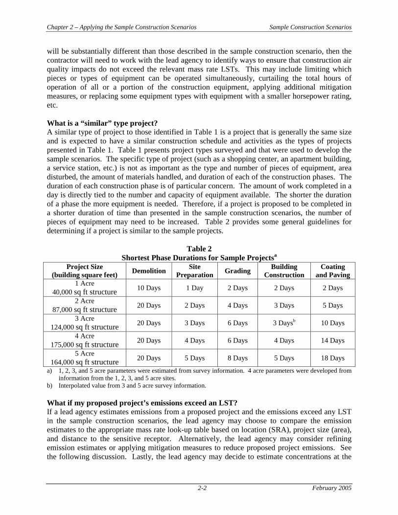
will be substantially different than those described in the sample construction scenario, then the contractor will need to work with the lead agency to identify ways to ensure that construction air quality impacts do not exceed the relevant mass rate LSTs. This may include limiting which pieces or types of equipment can be operated simultaneously, curtailing the total hours of operation of all or a portion of the construction equipment, applying additional mitigation measures, or replacing some equipment types with equipment with a smaller horsepower rating, etc. What is a “similar” type project? A similar type of project to those identified in Table 1 is a project that is generally the same size and is expected to have a similar construction schedule and activities as the types of projects presented in Table 1. Table 1 presents project types surveyed and that were used to develop the sample scenarios. The specific type of project (such as a shopping center, an apartment building, a service station, etc.) is not as important as the type and number of pieces of equipment, area disturbed, the amount of materials handled, and duration of each of the construction phases. The duration of each construction phase is of particular concern. The amount of work completed in a day is directly tied to the number and capacity of equipment available. The shorter the duration of a phase the more equipment is needed. Therefore, if a project is proposed to be completed in a shorter duration of time than presented in the sample construction scenarios, the number of pieces of equipment may need to be increased. Table 2 provides some general guidelines for determining if a project is similar to the sample projects.
Table 2 Shortest Phase Durations for Sample Projectsa
Project Size (building square feet) Demolition Site
Preparation Grading Building Construction
Coating and Paving
1 Acre 40,000 sq ft structure 10 Days 1 Day 2 Days 2 Days 2 Days
2 Acre 87,000 sq ft structure 20 Days 2 Days 4 Days 3 Days 5 Days
3 Acre 124,000 sq ft structure 20 Days 3 Days 6 Days 3 Daysb 10 Days
4 Acre 175,000 sq ft structure 20 Days 4 Days 6 Days 4 Days 14 Days
5 Acre 164,000 sq ft structure 20 Days 5 Days 8 Days 5 Days 18 Days
a) 1, 2, 3, and 5 acre parameters were estimated from survey information. 4 acre parameters were developed from information from the 1, 2, 3, and 5 acre sites.
b) Interpolated value from 3 and 5 acre survey information. What if my proposed project’s emissions exceed an LST? If a lead agency estimates emissions from a proposed project and the emissions exceed any LST in the sample construction scenarios, the lead agency may choose to compare the emission estimates to the appropriate mass rate look-up table based on location (SRA), project size (area), and distance to the sensitive receptor. Alternatively, the lead agency may consider refining emission estimates or applying mitigation measures to reduce proposed project emissions. See the following discussion. Lastly, the lead agency may decide to estimate concentrations at the
Chapter 2 – Applying the Sample Construction Scenarios Sample Construction Scenarios
2-3 February 2005
receptors around the proposed project-site using an air dispersion model such as ISCST3. Lead agencies that choose dispersion modeling should follow the approach presented in the Draft Localize Significance Threshold Methodology. How do I find the project specific LST? The LSTs presented in the sample construction scenarios are the “worst-case” LSTs. The “worst-case” is the lowest allowable mass emission based on standard modeling meteorological data, the highest pollutant concentration measured at the nearest ambient air quality monitoring station over the past three years3 (or 10.4 micrograms per cubic meter for construction PM10 and 2.5 micrograms per cubic meter for operational PM10), and with receptors 25 meters or closer to the propose project site. LSTs are dependent on the proposed project acreage, ambient air quality, meteorological data, and distance to the receptor. The lead agency may choose use the emission calculations in the sample construction scenarios, but use the mass rate look-up tables to determine the LSTs for the source receptor area where the proposed project is to be located according to project size and distance to the sensitive receptor. To find the LSTs for the source receptor area where the project is located, the lead agency would need to know the city where the proposed project would be located. The lead agency would use the table in Appendix I to find the source receptor area from the city where the proposed project would reside. Second, the lead agency would use the SRA to locate the LSTs from the mass rate LST look up tables by project acreage. For example, a one-acre office building is proposed to be constructed in Pasadena, where the nearest receptor is 100 meters away. According to Appendix I, Pasadena is in Source Receptor Area 8 – West San Gabriel Valley. The LSTs associated with Source Receptor Area 8 (NOx = 134 pounds per day, CO = 925 pounds per day, and PM10 = 85 pounds per day) may be used in place of the “worst-case” LSTs presented in the sample construction scenarios. The regional significance thresholds are 100 pounds per day of NOx, less than 550 pounds per day of CO, less than 75 pounds per day of VOC, less than 150 pounds of SOx, and less than 150 pounds per day of PM10. The NOx and CO LSTs are greater than the regional significance thresholds of 100 pounds per day of NOx and 550 pounds per day of CO. The only LST that is more stringent than a regional significance threshold is the PM10 LST of 85 pounds per day of PM10 (the regional significance threshold is 150 pounds per day of PM10). To be considered less than significant, the proposed project may not exceed the localized significance thresholds and the regional significance thresholds. In this example, if PM10 emissions are less than 150 pounds per day, but exceed the localized significance threshold (85 pounds per day) the proposed project would be considered significant for localized PM10 air quality impacts. What actions can be taken to reduce emission impacts by refining emission estimates? The lead agency should determine which pollutants exceed the applicable LSTs and focus on refining emission estimates for those pollutants. The most restrictive LST is the PM10 LST, since the district is non-attainment for PM10. Therefore, it is likely that if the project exceeds an
3 The highest concentration over the last three years was used for all source receptor areas except for SRA 7 -East
San Fernando Valley and SRA – 29 Banning Airport, because of nearby large single sources or events affecting the monitoring data. For these two source receptor areas the concentration for the last reported year (2003) was used.
Chapter 2 – Applying the Sample Construction Scenarios Sample Construction Scenarios
2-4 February 2005
LST, it would be the PM10 LST. It is possible that the proposed project may exceed more than one LST (e.g., PM10 and NOx). Emission estimates can be refined by using more precise methodologies, emission factors or project specific parameters. The emission methodologies presented in the sample construction scenarios are generic methodologies developed by EPA, CARB and SCAQMD. Lead agencies can use alternative methodologies or emission factors to estimate emissions. However, the lead agency should reference any alternative methodologies and emission factors used, and provide sufficient documentation so that the public can easily follow the emission estimation. The parameters presented in the sample construction scenarios are generic parameters developed by USEPA, CARB and SCAQMD. The lead agency may also substitute project specific parameters. For example, the silt content and moisture content used in the sample construction scenarios were taken from USEPA’s AP-42. These values may be replaced by project specific silt content and moisture content. The maximum daily average wind speeds were developed by the SCAQMD from meteorological data across all source receptor areas. Lead agencies may use the maximum daily average wind speeds for the proposed projects specific source receptor area. Vehicle speeds, capacities and on-site distances traveled were based on assumption. Lead agencies may develop vehicle speeds, capacities and on-site distances based on project specific data. The amount of area disturbed, dirt and debris handled and equipment profiles were developed from construction surveys. Lead agencies may replace these parameters with project specific data. In addition, lead agencies may also decide to adjust construction equipment hours, or the number or type of equipment on-site at any given time. Reducing the length of time certain pieces of equipment are used each day, amount of equipment operated each day, or the types of equipment that can be operated at the same time may reduce emissions. For example, if a project proponent requires both a bulldozer and a grader, but knows that neither will be on-site at the same time; the lead agency may estimate daily emissions for operations with bulldozer and graders separately. These two sets of independent emission estimates can then be compared separtely to the LSTs. What actions can be taken to reduce emission impacts? The lead agency should determine which pollutants exceed the applicable LST and focus on mitigation for those pollutants. The most restrictive LST is the PM10 LST, since the district is in non-attainment for PM10. Therefore, it is likely that if the project exceeds an LST, it would be the PM10 LST. It is possible that the proposed project may exceed more than one LST (e.g., PM10 and NOx). The LST mass rate look-up tables do contain dust suppression techniques required by SCAQMD Rule 403. Rule 403 requirements must be met by all projects and are not considered mitigation. Therefore, the sample construction scenario emission estimates are considered unmitigated. A list of possible mitigation measures beyond Rule 403 requirements are presented in Appendix H of this document. The mitigation measures chosen by lead agencies should then be included in an approved mitigation monitoring plan.
Chapter 2 – Applying the Sample Construction Scenarios Sample Construction Scenarios
2-5 February 2005
What if the propose project acreage is between the project acreages on the LST mass rate look-up tables? In this situation, the lead agency has two options. The first and easiest option would be to use the sample construction scenario and LSTs for acreage that is smaller than the proposed project. For example, if the proposed project is 2.5 acres, then use the two-acre sample construction scenario and LSTs. The second option would be to develop LSTs from a ratio of the known LSTs for the smaller and larger acreages. For example, if the proposed project is 3.7 acres, then LSTs for 3.7 acres can be predicted from three and four acre mass rate LST look-up table values by a ratio of the areas. Appendix K contains a methodology for estimating the LSTs by linear regression. If the second option is chosen, the sample construction scenario worksheets should be modified to reflect the 3.7-acre site. Either the three or the four acre sample construction scenario workbook can be used as a template. Each construction phase worksheet should be adjusted to reflect the 3.7 acre site. The structure dimensions in demolition and construction should be changed to project specific dimensions. The area disturbed in the site preparation and grading phases should be changed with project specific dimensions. The time length of each phase should be adjusted with project specific information. The amount of dirt and debris handled should be changed in the site preparation and grading phases. The truck trips and vehicle distance for trucks and bulldozers will change automatically when the area disturbed is changed in the site preparation and grading phases. The amount of demolition, debris handled, and truck trips in the demolition phase will change automatically when the size of the building is changed. The type and number of equipment, hours of operation and crew sizes should be adjusted with project specific information in each phase. If any of these values are not known, the lead agency may decide to approximate these values through linear regression from the three or four acre sample construction scenario values. Lead agencies may chose to alter any other methodology, emission factor or parameter to better reflect the actual project characteristics. What if a scenario for a larger project has more similarities to my project than the scenario for the actual size of my project? The project proponent may use a larger scenario or phase of a larger scenario to represent their project. However, the project proponent would be required to compare the emission estimates from the larger scenario with the mass rate LSTs associated with the proposed project size. The lead agency would need to estimate emissions using site-specific parameters. The easiest method would be to modify the example scenario spreadsheets with project specific parameters. See the procedures outlined in the second method of using the sample construction scenarios under the Sample Construction Scenarios section in Chapter 1. For example, if the amount of earth proposed to be moved in a two-acre project may be similar to the amount of earth moved in the three acre scenario, then the three-acre scenario can be used as a surrogate or modified with project specific information. The emissions from the sample scenario used to represent the proposed project or modified three-acre scenario would be compared to the two-acre mass rate LSTs, since the project is actually two-acres.
Chapter 2 – Applying the Sample Construction Scenarios Sample Construction Scenarios
2-6 February 2005
Why weren’t the scenarios designed to be “worst-case” options maximizing emissions? The sample construction scenarios were developed as average “worst-case” scenarios. SCAQMD developed parameters used in the scenarios from a construction site survey (see Pilot Study in Chapter 1 of this document). The survey provided information from approximately 50 sites, across SCAQMD jurisdiction, over a variety of project types. SCAQMD staff used the shortest number of days for phase completion (Table 2); and the upper ranges of areas disturbed, structure dimensions, areas paved, debris handled, etc. The average numbers of pieces of equipment, types of equipment, and operation hours were used. By using the shorter number of days per phase; the upper ranges of activities, areas disturbed and materials handled; and the average activity and number of pieces of equipment used an average “worst-case” was developed. Since SCAQMD staff believes that the survey was representative of the projects under its jurisdiction and the average “worst-case” parameters were used to estimate emissions, few projects are expected to generate more emissions. Therefore, the emissions presented in the scenarios are likely “worst-case,” since they represent actual construction activities. It is difficult to develop the absolute “worst-case” scenario that has emissions that are only slightly below the LSTs, since there are many combinations of equipment, operation and material handling. SCAQMD staff developed one-, two- and five-acre scenarios for the October 2003 Governing Board Meeting based on “worst-case” parameters from building and construction estimators. The building industry stated that building and construction estimators use national averages that do not adequately represent Southern California. The use of survey data addresses the building industries’ concerns. Can the mass rate LST look-up tables be used to evaluate multi-storied structures? Yes, in general the mass rate LST look-up tables can be used to evaluate multi-storied structures. Multi-storied structures were included in the construction survey. Demolition is directly related to structure size, since the amount of building debris handled is estimated from the volume of the building. Therefore, lead agencies should verify that the structure demolished is less than 50 feet tall as presented in the sample constructions scenarios. If the size of the proposed structure to be demolished, the amount and type of equipment is similar and the number of days spent demolishing the structure is equivalent or less, then the sample scenario can be used to represent the proposed project demolition phase. If the proposed project parameters are greater, the lead agency should modify the spreadsheets accordingly. The size of the structure in the structure construction phase is not directly related to the emissions. The size of the structure is related to the amount and types of construction equipment used in the survey. However, if a project builds a larger structure using the same amount of equipment, the same amount of emissions should be generated. Therefore, the amount, types and operating hours of the equipment are more accurate predictors of emissions in the structure construction phase. Consequently, the lead agency should use the construction equipment parameters as a gauge to whether or not a proposed project can be represented by a sample construction scenario.
Chapter 2 – Applying the Sample Construction Scenarios Sample Construction Scenarios
2-7 February 2005
However, if the structure is multi-storied, because it includes below ground levels; the sample construction scenarios would not apply. The sample construction scenarios only consider dirt and debris hauling from grading and clearing operations. Excavation would require more equipment and more haul trips. Lead agencies or project proponents would be expected to estimate emissions for excavation. Why do the scenarios use un-realistically large parameters? Some of the parameters used in the sample construction scenarios are larger than those typically allowed by regulation or practice. For example, most planning commissions will not allow buildings to occupy the entire lot, but require a certain amount of parking, landscaping and sidewalks. The survey forms were populated with check boxes to allow ease in completing the forms and to aid participants in completing the forms with the appropriate information in a prompt and consistent fashion. However, one disadvantage with using the check boxes was that for categories with large values ranges were used, such as building foot print, asphalt area, concrete area, area disturbed, dirt or debris handled, or distance traveled. Number of days each phase lasted, number of pieces of equipment, hours operated per day, and horsepower ratings were collected as discrete numbers. SCAQMD staff used the higher value in the range unless, the higher value was not appropriate. For example, one range for the building footprint is 41,000 to 60,000 square feet. However, one acre is approximately 43,000 feet. Therefore, if the proposed site is one acre then the maximum physical footprint area approximately 43,000 square feet. In practice, the city or county building codes may not allow a project proponent to build a structure that completely fills the site. By using the upper limits of the ranges the emissions are conservatively estimated. Where these values are greater than allowed by city or county building code, the project emissions would likely be less than those in the sample construction scenarios. Since the sample construction scenario emissions are below the LSTs, projects that generate less emission than the sample construction scenarios would also be less than significant for construction emissions. Why do the structure size and paving parameters appear to contradict each other? The structure area on the one-, two-, and three- acre sample construction scenarios are approximately the same size as the site area; and the pavers are reported to operate six to eight hours per day. These parameters are consistent with the site area. However, as stated earlier, the parameters used to develop the sample construction scenarios were obtained from the construction survey. The parameters are the average “worst-case” values developed per phase not by project. Therefore, the “worst-case” structure construction might not have included paving and the “worst-case” paving phase might have included paving a site to be used as a parking lot. Therefore, it is not expected that all of the information between phases would be consistent. But, by using the average “worst-case” values, the sample construction scenarios should represent most proposed projects less than five acres in the SCAQMD’s jurisdiction.
Chapter 2 – Applying the Sample Construction Scenarios Sample Construction Scenarios
2-8 February 2005
Where should the emission estimates and localized air quality impact analysis be presented? The sample construction scenarios used to represent a proposed project, the modified spreadsheets or project specific analysis should be included as an attachment or appendix to the CEQA document. A detailed explanation of why the sample construction scenarios are appropriate to be used to represent the proposed project, or how the sample construction scenarios were modified with site specific information, or documentation of the project specific analysis should also be included. The explanation should present enough detail for other agencies or the public to understand what was done and why it was appropriate. A summary of the analysis and conclusions should be included in the text of the CEQA document. Any additional mitigation or restrictions on activities or equipment should be clearly presented in the text of the CEQA document and in the mitigation monitoring plan. What if I need further assistance? Further assistance can be found by contacting the SCAQMD CEQA Section at (909) 396-3109 or submitting an e-mail to [email protected].

Sample Construction Scenarios
February 2005
A P P E N D I X A - O N E A C R E S I T E E X A M P L E
SUMMARY OF ONE ACRE SITE EXAMPLE RESULTS BY PHASE
SUMMARY OF ONE ACRE SITE EXAMPLE EQUIPMENT PARAMETE RS
SUMMARY OF ONE ACRE SITE RESULTS BY PHASE AND EQUIPMENT
ONE ACRE EXAMPLE
Demolition
Site Preparation
Grading
Building
Architectural Coating and Paving

Sample Construction Scenarios
February 2005
A P P E N D I X B - T W O A C R E S I T E E X A M P L E
SUMMARY OF TWO ACRE SITE EXAMPLE RESULTS BY PHASE
SUMMARY OF TWO ACRE SITE EXAMPLE EQUIPMENT PARAMETE RS
SUMMARY OF TWO ACRE SITE RESULTS BY PHASE AND EQUIP MENT
TWO ACRE EXAMPLE
Demolition
Site Preparation
Grading
Building
Architectural Coating and Paving
Sample Construction Scenarios
February 2005
A P P E N D I X C - T H R E E A C R E S I T E E X A M P L E
SUMMARY OF THREE ACRE SITE EXAMPLE RESULTS BY PHASE
SUMMARY OF THREE ACRE SITE EXAMPLE EQUIPMENT PARAME TERS
SUMMARY OF THREE ACRE SITE RESULTS BY PHASE AND EQU IPMENT
THREE ACRE EXAMPLE
Demolition
Site Preparation
Grading
Building
Architectural Coating and Paving
Sample Construction Scenarios
February 2005
A P P E N D I X D - F O U R A C R E S I T E E X A M P L E
SUMMARY OF FOUR ACRE SITE EXAMPLE RESULTS BY PHASE
SUMMARY OF FOUR ACRE SITE EXAMPLE EQUIPMENT PARAMET ERS
SUMMARY OF FOUR ACRE SITE RESULTS BY PHASE AND EQUI PMENT
FOUR ACRE EXAMPLE
Demolition
Site Preparation
Grading
Building
Architectural Coating and Paving

Sample Construction Scenarios
February 2005
A P P E N D I X E - F I V E A C R E S I T E E X A M P L E
SUMMARY OF FIVE ACRE SITE EXAMPLE RESULTS BY PHASE
SUMMARY OF FIVE ACRE SITE EXAMPLE EQUIPMENT PARAMET ERS
SUMMARY OF FIVE ACRE SITE RESULTS BY PHASE AND EQUI PMENT
FIVE ACRE EXAMPLE
Demolition
Site Preparation
Grading
Building
Architectural Coating and Paving
Sample Construction Scenarios
February 2005
A P P E N D I X F - E X A M P L E C O N S T R U C T I O N E M I S S I O N E S T I M A T I O N D O C U M E N T A T I O N

Sample Construction Scenarios
F-1 February 2005
EXAMPLE CONSTRUCTION EMISSION ESTIMATION DOCUMENTAT IONa
Project Size (building footprint sqft)
Demolition Site Preparation
Grading Building Construction
Coating and Paving
1 Acre 40,000 sq ft building
10 Days 1 Day 2 Days 2 Days 2 Days
2 Acre 87,000 sq ft building
20 Days 2 Days 4 Days 3 Days 5 Days
3 Acre 124,000 sq ft building
20 Days 3 Days 6 Days 3 Daysb 10 Days
4 Acre 175,000 sq ft building
20 Days 4 Days 6 Days 4 Days 14 Days
5 Acre 164,000 sq ft building
20 Days 5 Days 8 Days 5 Days 18 Days
c) 1, 2, 3, and 5 acre parameters were estimated from survey information. 4 acre parameters were developed from information from the 1, 2, 3, and 5 acre sites.
d) Interpolated value. Shortest duration in survey was 110 days. SITE CHARACTERISTICS Project Size Demolition Site
Preparation Grading Building
Construction Coating and
Paving 1 Acre 41,000 sq ft
structure 40,000 sq ft disturbed
40,000 sq ft disturbed
41,000 sq ft structure
41,000 sq ft structure
2 Acre 87,000 sq ft structure
87,000 sq ft disturbed
87,000 sq ft disturbed
87,000 sq ft structure
87,000 sq ft structure
3 Acre 124,000 sq ft structure
130,000 sq ft disturbed
130,000 sq ft disturbed
124,000 sq ft structure
124,000 sq ft structure
4 Acre 150,000 sq ft structure
175,000 sq ft disturbed
175,000 sq ft disturbed
150,000 sq ft structure
150,000 sq ft structure
5 Acre 164,000 sq ft structure
200,000 sq ft disturbed
200,000 sq ft disturbed
164,000 sq ft structure
164,000 sq ft structure
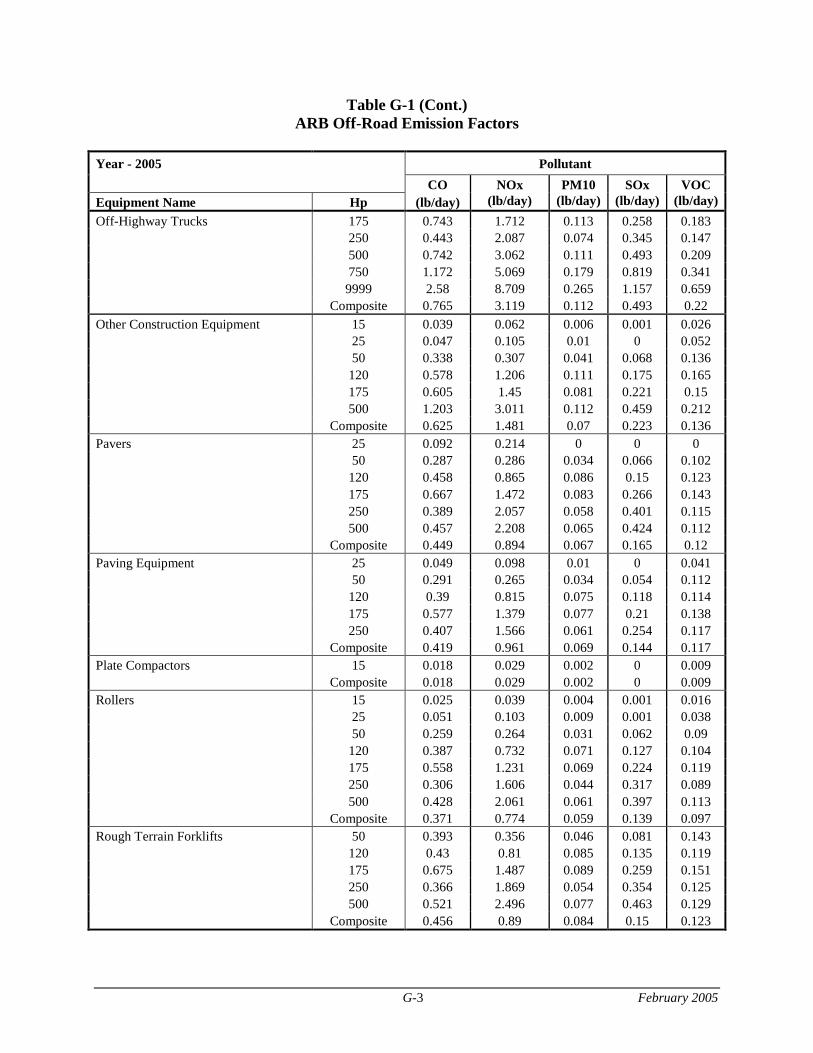
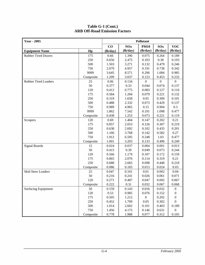
EMISSION CALCULATION SOURCES Off-Road Construction Equipment Emission calculations for off-road equipment are based on emission factors provided by the California Air Resource Board (ARB) from their Off-Road Mobile Source Model, which can be downloaded from the SCAQMD website at http://www.aqmd.gov/ceqa/hdbk.html. The emission factors included in Appendix G represent a composite emission factor for each off-road construction equipment category in units of pounds of emissions per hour. These off-road emission factors will replace the emission factors in the SCAQMD CEQA Air Quality Handbook (CEQA Handbook), September 1993, Tables A9-8-A and A9-8-B. The emission factors in Appendix G represent the overall fleet mix for the year specified, for each of the off-road construction equipment categories. The average horsepower and load factor
Sample Construction Scenarios
F-2 February 2005
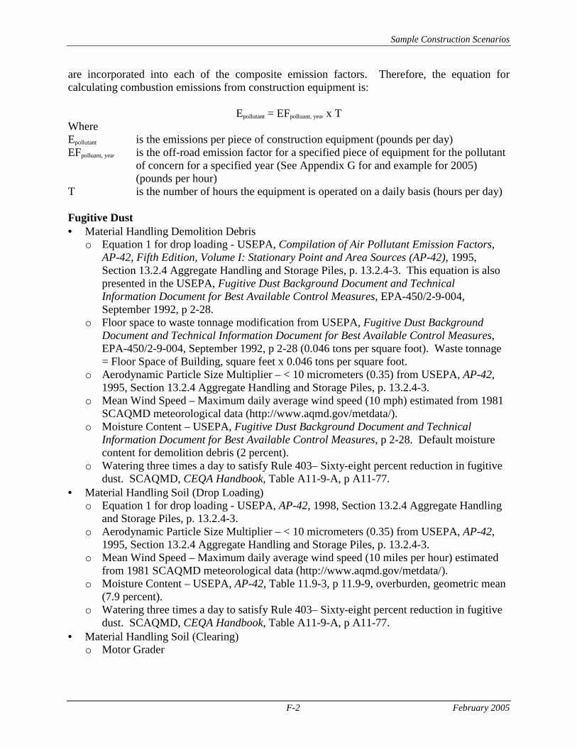
are incorporated into each of the composite emission factors. Therefore, the equation for calculating combustion emissions from construction equipment is:
Epollutant = EFpolluant, year x T Where Epollutant is the emissions per piece of construction equipment (pounds per day) EFpolluant, year is the off-road emission factor for a specified piece of equipment for the pollutant
of concern for a specified year (See Appendix G for and example for 2005) (pounds per hour)
T is the number of hours the equipment is operated on a daily basis (hours per day) Fugitive Dust • Material Handling Demolition Debris
o Equation 1 for drop loading - USEPA, Compilation of Air Pollutant Emission Factors, AP-42, Fifth Edition, Volume I: Stationary Point and Area Sources (AP-42), 1995, Section 13.2.4 Aggregate Handling and Storage Piles, p. 13.2.4-3. This equation is also presented in the USEPA, Fugitive Dust Background Document and Technical Information Document for Best Available Control Measures, EPA-450/2-9-004, September 1992, p 2-28.
o Floor space to waste tonnage modification from USEPA, Fugitive Dust Background Document and Technical Information Document for Best Available Control Measures, EPA-450/2-9-004, September 1992, p 2-28 (0.046 tons per square foot). Waste tonnage = Floor Space of Building, square feet x 0.046 tons per square foot.
o Aerodynamic Particle Size Multiplier – < 10 micrometers (0.35) from USEPA, AP-42, 1995, Section 13.2.4 Aggregate Handling and Storage Piles, p. 13.2.4-3.
o Mean Wind Speed – Maximum daily average wind speed (10 mph) estimated from 1981 SCAQMD meteorological data (http://www.aqmd.gov/metdata/).
o Moisture Content – USEPA, Fugitive Dust Background Document and Technical Information Document for Best Available Control Measures, p 2-28. Default moisture content for demolition debris (2 percent).
o Watering three times a day to satisfy Rule 403– Sixty-eight percent reduction in fugitive dust. SCAQMD, CEQA Handbook, Table A11-9-A, p A11-77.
• Material Handling Soil (Drop Loading) o Equation 1 for drop loading - USEPA, AP-42, 1998, Section 13.2.4 Aggregate Handling
and Storage Piles, p. 13.2.4-3. o Aerodynamic Particle Size Multiplier – < 10 micrometers (0.35) from USEPA, AP-42,
1995, Section 13.2.4 Aggregate Handling and Storage Piles, p. 13.2.4-3. o Mean Wind Speed – Maximum daily average wind speed (10 miles per hour) estimated
from 1981 SCAQMD meteorological data (http://www.aqmd.gov/metdata/). o Moisture Content – USEPA, AP-42, Table 11.9-3, p 11.9-9, overburden, geometric mean
(7.9 percent). o Watering three times a day to satisfy Rule 403– Sixty-eight percent reduction in fugitive
dust. SCAQMD, CEQA Handbook, Table A11-9-A, p A11-77. • Material Handling Soil (Clearing)
o Motor Grader
Sample Construction Scenarios
F-3 February 2005
� Equation for grading - USEPA, AP-42, 1998, Section 11.9 Western Surface Coal Mining, Table 11.9-1, p. 11.9-5. Grading.
� Vehicle Speed – Assumed to be 3 miles per hour. � Vehicle Miles Traveled – Estimated by assuming a 13-foot blade with a 2-foot
overlap (11-foot effective width) traveling over the area disturbed. o Bulldozer
� USEPA, AP-42, 1995, Table 11.9-1, p 11.9-5, equation for bulldozing, overburden, particulate less than 10 microns in aerodynamic diameter.
� Silt Content – USEPA, AP-42, Table 11.9-3, p 11.9-9, overburden, geometric mean (6.9 percent).
� Moisture Content – USEPA, AP-42, Table 11.9-3, p 11.9-9, overburden, geometric mean (7.9 percent).
� Watering three times a day to satisfy Rule 403– Sixty-eight percent reduction in fugitive dust. SCAQMD, CEQA Handbook, Table A11-9-A, p A11-77.
o Scraper � USEPA, AP-42, July 1998, Equation 1b and Table 13.2.2-2, AP-42, December 2003.
Also see comment g of Table 11.9-1. � Mean vehicle weight - estimated from 631G Model Scraper Caterpillar Performance
Handbook, Edition 33. Scraper in the same horsepower range (450-490 hp) as the composite ARB emission factors. (120,460 pound empty with a 75,000 pound capacity).
� Caterpiller G31G has a 11.5 foot wide blade, with an assumed 2 foot overlap (9.5 foot wide).
• Grading o Grader
� Equation for grading - USEPA, AP-42, 1998, Section 11.9 Western Surface Coal Mining, Table 11.9-1, p 11.9-5, Grading.
� Vehicle Speed – Assumed to be 3 mph. � Vehicle Miles Traveled – Estimated by assuming a 13-foot blade with a 2-foot
overlap (11-foot effective width) traveling over the area disturbed. � Watering three times a day to satisfy Rule 403– Sixty-eight percent reduction in
fugitive dust. SCAQMD, CEQA Handbook, Table A11-9-A, p A11-77. o Scraper
� USEPA, AP-42, July 1998, Equation 1b and Table 13.2.2-2, AP-42, December 2003. Also see comment g of Table 11.9-1.
� Mean vehicle weight - estimated from 631G Model Scraper Caterpillar Performance Handbook, Edition 33. Scraper in the same horsepower range (450-490 hp) as the composite ARB emission factors. (120,460 pound empty with a 75,000 pound capacity).
� Caterpiller G31G has a 11.5 foot wide blade, with an assumed 2 foot overlap (9.5 foot wide).
• Storage Piles o USEPA, Fugitive Dust Background Document and Technical Information Document for
Best Available Control Measures, Equation 2-12, p 2-25, also referenced in SCAQMD CEQA Handbook, Table A9-9-E, p A9-99.
Sample Construction Scenarios
F-4 February 2005
o Silt Content – USEPA, AP-42, Table 11.9-3, p 11.9-9, overburden, geometric mean (6.9 percent)
o Number of days with > 0.01 inches of precipitation per year - SCAQMD CEQA Handbook, Table A9-9-E-2, p A9-99.
o Percentage of time that the unobstructed wind speed exceeds 12 mph at mean pile height – 100% based on review of 1981 SCAQMD meteorological data (http://www.aqmd.gov/metdata/).
o Watering three times a day to satisfy Rule 403– Sixty-eight percent reduction in fugitive dust. SCAQMD, CEQA Handbook, Table A11-9-A, p A11-77.
• On-site, On-road Vehicle Travel o CARB, EMFAC2002 (version 2.2) Burden Model with the following options selected:
Winter season, 2005 calendar year, 75 ºF (2003 AQMP), 40 percent relative humidity (2003 AQMP).
o Number of Haul Truck Trips – Estimated from amount of dirt and debris moved by haul trucks with 30 cubic yard haul capacity over the time length of the construction phase.
o Haul Truck Miles Traveled On-site – Assumed to be 0.1 miles through facility. o Water Truck Miles Traveled On-site – Estimated by assuming a six foot wide truck
traveling over the area disturbed. SIGNIFICANCE THRESHOLDS • Regional significance thresholds from Chapter 6 of SCAQMD, CEQA Handbook, p 6-1
through p 6-4. • Localized significance thresholds from Attachment D - Draft Localized Significance
Threshold Methodology of Governing Board Agenda Item 36. Implement FY 2002-03 Environmental Justice Enhancement I – 4: Continue to Develop Localized Significance Thresholds for Subregions of the Air District as Another Indicator of CEQA Significance, July 11 2003. Most stringent of LST among all SRA for each site size category was used.

February 2005
A P P E N D I X G - A R B O F F - R O A D E M I S S I O N F A C T O R S
G-1 February 2005
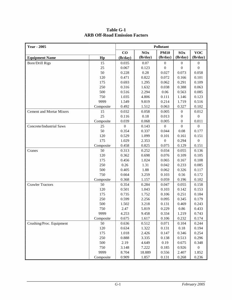
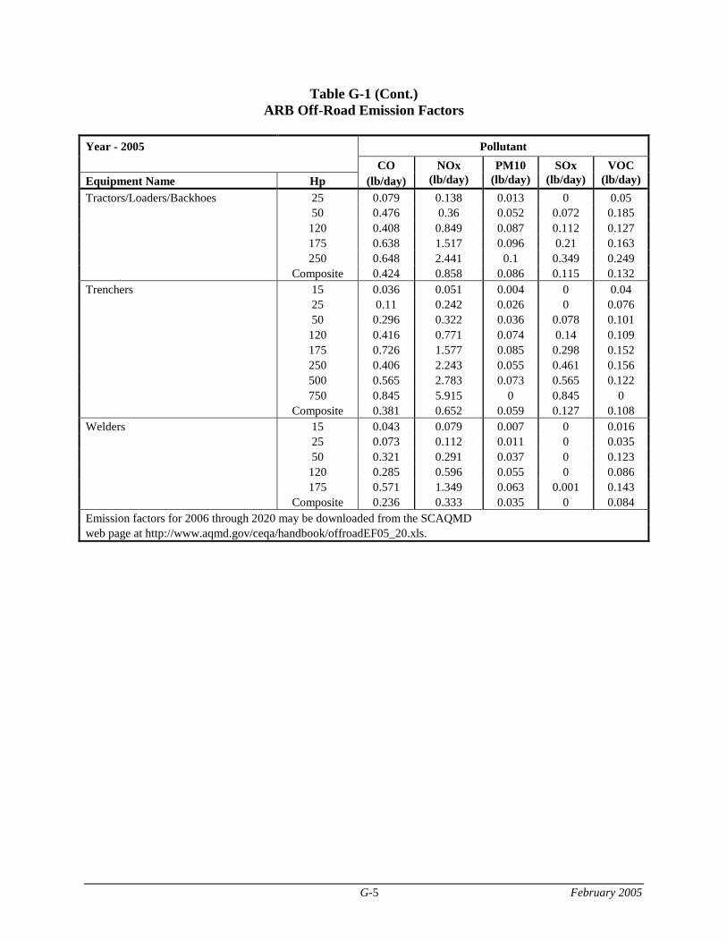
Table G-1 ARB Off-Road Emission Factors
Year - 2005 Pollutant
CO NOx PM10 SOx VOC Equipment Name Hp (lb/day) (lb/day) (lb/day) (lb/day) (lb/day)
Bore/Drill Rigs 15 0.035 0.07 0 0 0 25 0.067 0.123 0 0 0 50 0.228 0.28 0.027 0.073 0.058 120 0.471 0.822 0.072 0.166 0.101 175 0.693 1.295 0.062 0.291 0.109 250 0.316 1.632 0.038 0.388 0.063 500 0.516 2.294 0.06 0.563 0.085 750 1.035 4.806 0.111 1.146 0.123 9999 1.549 9.819 0.214 1.719 0.516 Composite 0.492 1.512 0.063 0.327 0.102 Cement and Mortar Mixers 15 0.032 0.058 0.005 0 0.012 25 0.116 0.18 0.013 0 0 Composite 0.039 0.068 0.005 0 0.011 Concrete/Industrial Saws 25 0 0.143 0 0 0 50 0.354 0.337 0.044 0.08 0.177 120 0.529 1.099 0.101 0.161 0.151 175 1.029 2.353 0 0.294 0 Composite 0.458 0.825 0.075 0.129 0.151 Cranes 50 0.313 0.252 0.034 0.055 0.136 120 0.362 0.698 0.076 0.109 0.105 175 0.456 1.024 0.065 0.167 0.108 250 0.26 1.31 0.042 0.233 0.085 500 0.405 1.88 0.062 0.326 0.117 750 0.664 3.259 0.103 0.56 0.172 Composite 0.368 1.157 0.059 0.196 0.102 Crawler Tractors 50 0.354 0.284 0.047 0.055 0.158 120 0.501 1.043 0.103 0.142 0.153 175 0.735 1.752 0.106 0.251 0.184 250 0.599 2.256 0.095 0.345 0.179 500 1.502 3.218 0.131 0.469 0.243 750 2.47 5.819 0.229 0.86 0.433 9999 4.253 9.458 0.334 1.219 0.743 Composite 0.675 1.617 0.106 0.232 0.174 Crushing/Proc. Equipment 50 0.636 0.512 0.071 0.104 0.244 120 0.634 1.322 0.131 0.18 0.194 175 1.018 2.426 0.147 0.346 0.254 250 0.888 3.335 0.138 0.513 0.296 500 2.19 4.649 0.19 0.675 0.348 750 3.148 7.222 0.185 0.926 0 9999 8.704 18.889 0.556 2.407 1.852 Composite 0.909 1.857 0.131 0.268 0.236
G-2 February 2005
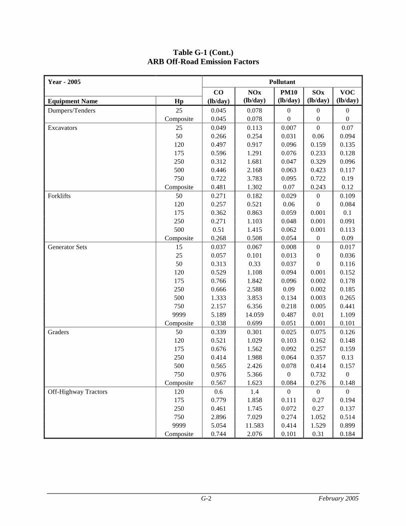
Table G-1 (Cont.) ARB Off-Road Emission Factors
Year - 2005 Pollutant
CO NOx PM10 SOx VOC Equipment Name Hp (lb/day) (lb/day) (lb/day) (lb/day) (lb/day)
Dumpers/Tenders 25 0.045 0.078 0 0 0 Composite 0.045 0.078 0 0 0 Excavators 25 0.049 0.113 0.007 0 0.07 50 0.266 0.254 0.031 0.06 0.094 120 0.497 0.917 0.096 0.159 0.135 175 0.596 1.291 0.076 0.233 0.128 250 0.312 1.681 0.047 0.329 0.096 500 0.446 2.168 0.063 0.423 0.117 750 0.722 3.783 0.095 0.722 0.19 Composite 0.481 1.302 0.07 0.243 0.12 Forklifts 50 0.271 0.182 0.029 0 0.109 120 0.257 0.521 0.06 0 0.084 175 0.362 0.863 0.059 0.001 0.1 250 0.271 1.103 0.048 0.001 0.091 500 0.51 1.415 0.062 0.001 0.113 Composite 0.268 0.508 0.054 0 0.09 Generator Sets 15 0.037 0.067 0.008 0 0.017 25 0.057 0.101 0.013 0 0.036 50 0.313 0.33 0.037 0 0.116 120 0.529 1.108 0.094 0.001 0.152 175 0.766 1.842 0.096 0.002 0.178 250 0.666 2.588 0.09 0.002 0.185 500 1.333 3.853 0.134 0.003 0.265 750 2.157 6.356 0.218 0.005 0.441 9999 5.189 14.059 0.487 0.01 1.109 Composite 0.338 0.699 0.051 0.001 0.101 Graders 50 0.339 0.301 0.025 0.075 0.126 120 0.521 1.029 0.103 0.162 0.148 175 0.676 1.562 0.092 0.257 0.159 250 0.414 1.988 0.064 0.357 0.13 500 0.565 2.426 0.078 0.414 0.157 750 0.976 5.366 0 0.732 0 Composite 0.567 1.623 0.084 0.276 0.148 Off-Highway Tractors 120 0.6 1.4 0 0 0 175 0.779 1.858 0.111 0.27 0.194 250 0.461 1.745 0.072 0.27 0.137 750 2.896 7.029 0.274 1.052 0.514 9999 5.054 11.583 0.414 1.529 0.899 Composite 0.744 2.076 0.101 0.31 0.184
G-3 February 2005
Table G-1 (Cont.) ARB Off-Road Emission Factors
Year - 2005 Pollutant
CO NOx PM10 SOx VOC Equipment Name Hp (lb/day) (lb/day) (lb/day) (lb/day) (lb/day)
Off-Highway Trucks 175 0.743 1.712 0.113 0.258 0.183 250 0.443 2.087 0.074 0.345 0.147 500 0.742 3.062 0.111 0.493 0.209 750 1.172 5.069 0.179 0.819 0.341 9999 2.58 8.709 0.265 1.157 0.659 Composite 0.765 3.119 0.112 0.493 0.22
Other Construction Equipment 15 0.039 0.062 0.006 0.001 0.026 25 0.047 0.105 0.01 0 0.052 50 0.338 0.307 0.041 0.068 0.136 120 0.578 1.206 0.111 0.175 0.165 175 0.605 1.45 0.081 0.221 0.15 500 1.203 3.011 0.112 0.459 0.212 Composite 0.625 1.481 0.07 0.223 0.136 Pavers 25 0.092 0.214 0 0 0 50 0.287 0.286 0.034 0.066 0.102 120 0.458 0.865 0.086 0.15 0.123 175 0.667 1.472 0.083 0.266 0.143 250 0.389 2.057 0.058 0.401 0.115 500 0.457 2.208 0.065 0.424 0.112 Composite 0.449 0.894 0.067 0.165 0.12 Paving Equipment 25 0.049 0.098 0.01 0 0.041 50 0.291 0.265 0.034 0.054 0.112 120 0.39 0.815 0.075 0.118 0.114 175 0.577 1.379 0.077 0.21 0.138 250 0.407 1.566 0.061 0.254 0.117 Composite 0.419 0.961 0.069 0.144 0.117 Plate Compactors 15 0.018 0.029 0.002 0 0.009 Composite 0.018 0.029 0.002 0 0.009 Rollers 15 0.025 0.039 0.004 0.001 0.016 25 0.051 0.103 0.009 0.001 0.038 50 0.259 0.264 0.031 0.062 0.09 120 0.387 0.732 0.071 0.127 0.104 175 0.558 1.231 0.069 0.224 0.119 250 0.306 1.606 0.044 0.317 0.089 500 0.428 2.061 0.061 0.397 0.113 Composite 0.371 0.774 0.059 0.139 0.097 Rough Terrain Forklifts 50 0.393 0.356 0.046 0.081 0.143 120 0.43 0.81 0.085 0.135 0.119 175 0.675 1.487 0.089 0.259 0.151 250 0.366 1.869 0.054 0.354 0.125 500 0.521 2.496 0.077 0.463 0.129 Composite 0.456 0.89 0.084 0.15 0.123
G-4 February 2005
Table G-1 (Cont.) ARB Off-Road Emission Factors
Year - 2005 Pollutant
CO NOx PM10 SOx VOC Equipment Name Hp (lb/day) (lb/day) (lb/day) (lb/day) (lb/day)
Rubber Tired Dozers 175 0.66 1.396 0.075 0.264 0.189 250 0.656 2.475 0.103 0.38 0.193 500 1.503 3.271 0.132 0.479 0.246 750 2.079 4.957 0.191 0.738 0.342 9999 3.645 8.571 0.296 1.084 0.985 Composite 1.209 3.037 0.123 0.453 0.232 Rubber Tired Loaders 25 0.06 0.134 0 0 0 50 0.377 0.33 0.044 0.074 0.137 120 0.412 0.775 0.083 0.127 0.116 175 0.584 1.284 0.079 0.221 0.132 250 0.319 1.658 0.05 0.309 0.101 500 0.488 2.332 0.073 0.429 0.137 750 0.989 4.965 0.15 0.904 0.3 9999 1.862 7.542 0.191 1.098 0.477 Composite 0.438 1.253 0.073 0.221 0.119 Scrapers 120 0.69 1.404 0.147 0.202 0.21 175 0.857 2.053 0.126 0.307 0.219 250 0.638 2.692 0.102 0.435 0.201 500 1.166 3.768 0.142 0.582 0.27 750 1.912 6.595 0.248 1.03 0.477 Composite 1.001 3.203 0.133 0.496 0.249 Signal Boards 15 0.024 0.037 0.004 0.001 0.013 50 0.415 0.39 0.049 0.073 0.244 120 0.566 1.179 0.107 0.172 0.159 175 0.865 2.076 0.114 0.319 0.21 250 0.688 2.665 0.098 0.448 0.218 Composite 0.086 0.183 0.013 0.024 0.03 Skid Steer Loaders 25 0.047 0.101 0.01 0.002 0.04 50 0.216 0.241 0.026 0.061 0.071 120 0.271 0.487 0.047 0.092 0.067 Composite 0.222 0.31 0.032 0.067 0.068 Surfacing Equipment 50 0.159 0.143 0.016 0.032 0 120 0.53 0.985 0.076 0.152 0 175 0.505 1.212 0 0.202 0 250 0.452 1.709 0.05 0.302 0 500 1.014 2.602 0.101 0.403 0.189 750 1.456 4.175 0.146 0.631 0 Composite 0.778 1.988 0.077 0.312 0.105
G-5 February 2005
Table G-1 (Cont.) ARB Off-Road Emission Factors
Year - 2005 Pollutant
CO NOx PM10 SOx VOC Equipment Name Hp (lb/day) (lb/day) (lb/day) (lb/day) (lb/day)
Tractors/Loaders/Backhoes 25 0.079 0.138 0.013 0 0.05 50 0.476 0.36 0.052 0.072 0.185 120 0.408 0.849 0.087 0.112 0.127 175 0.638 1.517 0.096 0.21 0.163 250 0.648 2.441 0.1 0.349 0.249 Composite 0.424 0.858 0.086 0.115 0.132 Trenchers 15 0.036 0.051 0.004 0 0.04 25 0.11 0.242 0.026 0 0.076 50 0.296 0.322 0.036 0.078 0.101 120 0.416 0.771 0.074 0.14 0.109 175 0.726 1.577 0.085 0.298 0.152 250 0.406 2.243 0.055 0.461 0.156 500 0.565 2.783 0.073 0.565 0.122 750 0.845 5.915 0 0.845 0 Composite 0.381 0.652 0.059 0.127 0.108 Welders 15 0.043 0.079 0.007 0 0.016 25 0.073 0.112 0.011 0 0.035 50 0.321 0.291 0.037 0 0.123 120 0.285 0.596 0.055 0 0.086 175 0.571 1.349 0.063 0.001 0.143 Composite 0.236 0.333 0.035 0 0.084 Emission factors for 2006 through 2020 may be downloaded from the SCAQMD web page at http://www.aqmd.gov/ceqa/handbook/offroadEF05_20.xls.

February 2005
A P P E N D I X H - P O S S I B L E M I T A G A T I O N M E A S U R E S
H-1 February 2005
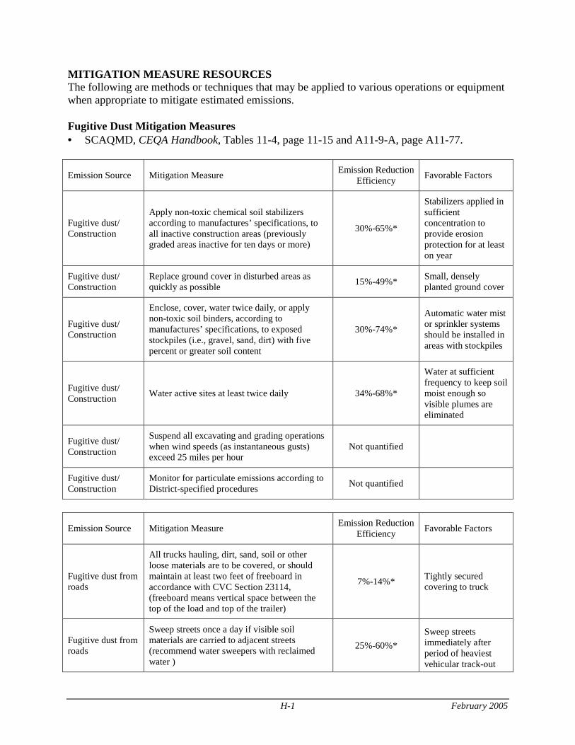
MITIGATION MEASURE RESOURCES The following are methods or techniques that may be applied to various operations or equipment when appropriate to mitigate estimated emissions. Fugitive Dust Mitigation Measures • SCAQMD, CEQA Handbook, Tables 11-4, page 11-15 and A11-9-A, page A11-77.
Emission Source Mitigation Measure Emission Reduction
Efficiency Favorable Factors
Fugitive dust/ Construction
Apply non-toxic chemical soil stabilizers according to manufactures’ specifications, to all inactive construction areas (previously graded areas inactive for ten days or more)
30%-65%*
Stabilizers applied in sufficient concentration to provide erosion protection for at least on year
Fugitive dust/ Construction
Replace ground cover in disturbed areas as quickly as possible
15%-49%* Small, densely planted ground cover
Fugitive dust/ Construction
Enclose, cover, water twice daily, or apply non-toxic soil binders, according to manufactures’ specifications, to exposed stockpiles (i.e., gravel, sand, dirt) with five percent or greater soil content
30%-74%*
Automatic water mist or sprinkler systems should be installed in areas with stockpiles
Fugitive dust/ Construction
Water active sites at least twice daily 34%-68%*
Water at sufficient frequency to keep soil moist enough so visible plumes are eliminated
Fugitive dust/ Construction
Suspend all excavating and grading operations when wind speeds (as instantaneous gusts) exceed 25 miles per hour
Not quantified
Fugitive dust/ Construction
Monitor for particulate emissions according to District-specified procedures
Not quantified
Emission Source Mitigation Measure Emission Reduction
Efficiency Favorable Factors
Fugitive dust from roads
All trucks hauling, dirt, sand, soil or other loose materials are to be covered, or should maintain at least two feet of freeboard in accordance with CVC Section 23114, (freeboard means vertical space between the top of the load and top of the trailer)
7%-14%* Tightly secured covering to truck
Fugitive dust from roads
Sweep streets once a day if visible soil materials are carried to adjacent streets (recommend water sweepers with reclaimed water )
25%-60%*
Sweep streets immediately after period of heaviest vehicular track-out
H-2 February 2005
activity
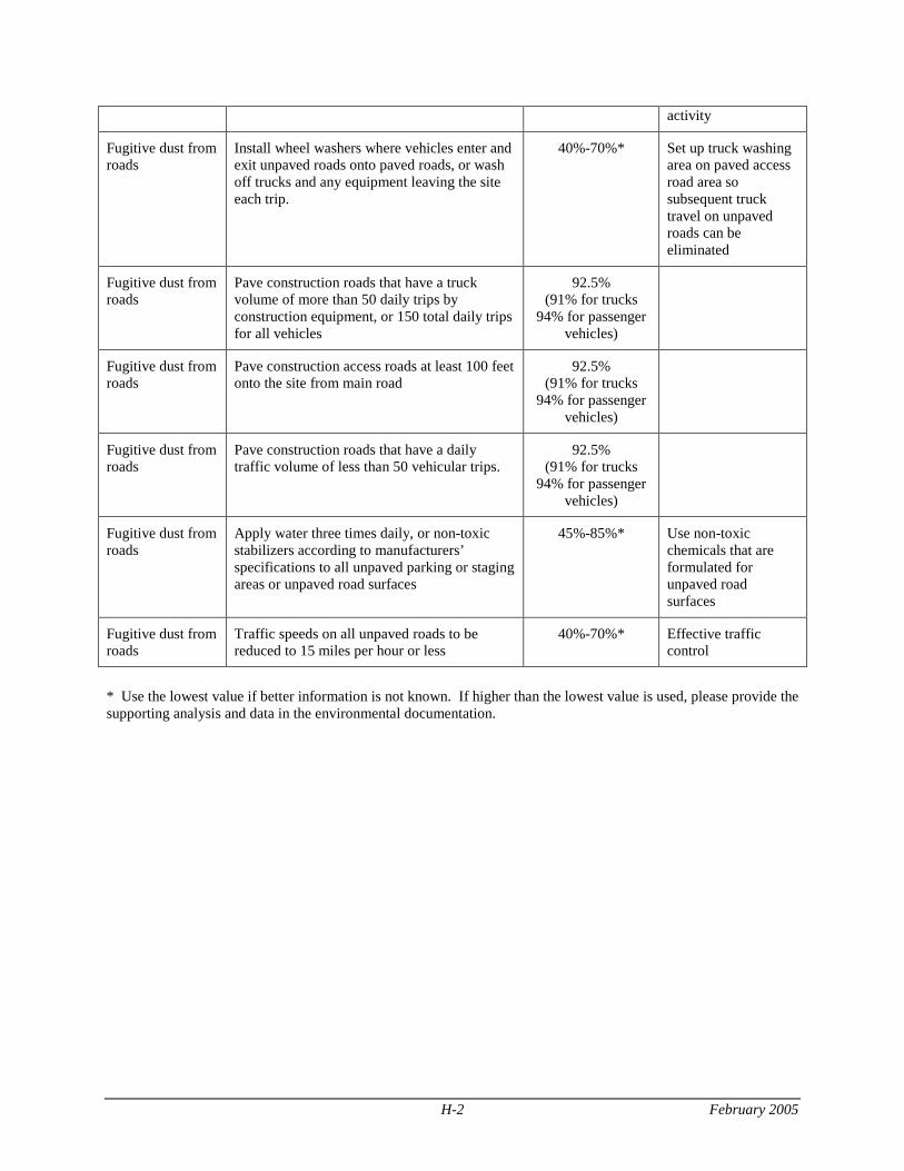
Fugitive dust from roads
Install wheel washers where vehicles enter and exit unpaved roads onto paved roads, or wash off trucks and any equipment leaving the site each trip.
40%-70%* Set up truck washing area on paved access road area so subsequent truck travel on unpaved roads can be eliminated
Fugitive dust from roads
Pave construction roads that have a truck volume of more than 50 daily trips by construction equipment, or 150 total daily trips for all vehicles
92.5% (91% for trucks
94% for passenger vehicles)
Fugitive dust from roads
Pave construction access roads at least 100 feet onto the site from main road
92.5% (91% for trucks
94% for passenger vehicles)
Fugitive dust from roads
Pave construction roads that have a daily traffic volume of less than 50 vehicular trips.
92.5% (91% for trucks
94% for passenger vehicles)
Fugitive dust from roads
Apply water three times daily, or non-toxic stabilizers according to manufacturers’ specifications to all unpaved parking or staging areas or unpaved road surfaces
45%-85%* Use non-toxic chemicals that are formulated for unpaved road surfaces
Fugitive dust from roads
Traffic speeds on all unpaved roads to be reduced to 15 miles per hour or less
40%-70%* Effective traffic control
* Use the lowest value if better information is not known. If higher than the lowest value is used, please provide the supporting analysis and data in the environmental documentation.
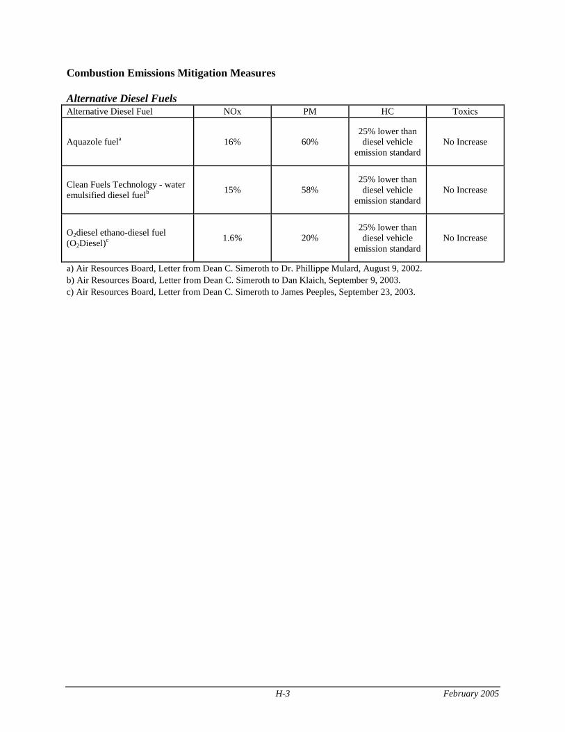
H-3 February 2005
Combustion Emissions Mitigation Measures Alternative Diesel Fuels Alternative Diesel Fuel NOx PM HC Toxics
Aquazole fuela 16% 60% 25% lower than diesel vehicle
emission standard No Increase
Clean Fuels Technology - water emulsified diesel fuelb
15% 58% 25% lower than diesel vehicle
emission standard No Increase
O2diesel ethano-diesel fuel (O2Diesel)c
1.6% 20% 25% lower than diesel vehicle
emission standard No Increase
a) Air Resources Board, Letter from Dean C. Simeroth to Dr. Phillippe Mulard, August 9, 2002. b) Air Resources Board, Letter from Dean C. Simeroth to Dan Klaich, September 9, 2003. c) Air Resources Board, Letter from Dean C. Simeroth to James Peeples, September 23, 2003.

February 2005
A P P E N D I X I - S O U R C E R E C E P T O R A R E A B Y C I T Y
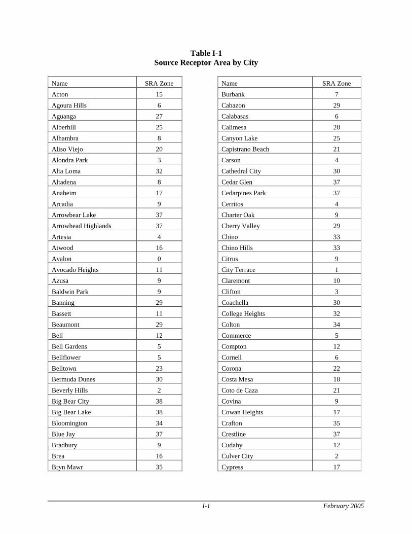
I-1 February 2005
Table I-1 Source Receptor Area by City
Name SRA Zone
Acton 15
Agoura Hills 6
Aguanga 27
Alberhill 25
Alhambra 8
Aliso Viejo 20
Alondra Park 3
Alta Loma 32
Altadena 8
Anaheim 17
Arcadia 9
Arrowbear Lake 37
Arrowhead Highlands 37
Artesia 4
Atwood 16
Avalon 0
Avocado Heights 11
Azusa 9
Baldwin Park 9
Banning 29
Bassett 11
Beaumont 29
Bell 12
Bell Gardens 5
Bellflower 5
Belltown 23
Bermuda Dunes 30
Beverly Hills 2
Big Bear City 38
Big Bear Lake 38
Bloomington 34
Blue Jay 37
Bradbury 9
Brea 16
Bryn Mawr 35
Name SRA Zone
Burbank 7
Cabazon 29
Calabasas 6
Calimesa 28
Canyon Lake 25
Capistrano Beach 21
Carson 4
Cathedral City 30
Cedar Glen 37
Cedarpines Park 37
Cerritos 4
Charter Oak 9
Cherry Valley 29
Chino 33
Chino Hills 33
Citrus 9
City Terrace 1
Claremont 10
Clifton 3
Coachella 30
College Heights 32
Colton 34
Commerce 5
Compton 12
Cornell 6
Corona 22
Costa Mesa 18
Coto de Caza 21
Covina 9
Cowan Heights 17
Crafton 35
Crestline 37
Cudahy 12
Culver City 2
Cypress 17
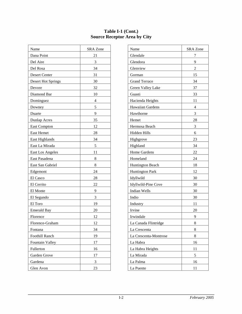
I-2 February 2005
Table I-1 (Cont.) Source Receptor Area by City
Name SRA Zone
Dana Point 21
Del Aire 3
Del Rosa 34
Desert Center 31
Desert Hot Springs 30
Devore 32
Diamond Bar 10
Dominguez 4
Downey 5
Duarte 9
Dunlap Acres 35
East Compton 12
East Hemet 28
East Highlands 34
East La Mirada 5
East Los Angeles 11
East Pasadena 8
East San Gabriel 8
Edgemont 24
El Casco 28
El Cerrito 22
El Monte 9
El Segundo 3
El Toro 19
Emerald Bay 20
Florence 12
Florence-Graham 12
Fontana 34
Foothill Ranch 19
Fountain Valley 17
Fullerton 16
Garden Grove 17
Gardena 3
Glen Avon 23
Name SRA Zone
Glendale 7
Glendora 9
Glenview 2
Gorman 15
Grand Terrace 34
Green Valley Lake 37
Guasti 33
Hacienda Heights 11
Hawaiian Gardens 4
Hawthorne 3
Hemet 28
Hermosa Beach 3
Hidden Hills 6
Highgrove 23
Highland 34
Home Gardens 22
Homeland 24
Huntington Beach 18
Huntington Park 12
Idyllwild 30
Idyllwild-Pine Cove 30
Indian Wells 30
Indio 30
Industry 11
Irvine 20
Irwindale 9
La Canada Flintridge 8
La Crescenta 8
La Crescenta-Montrose 8
La Habra 16
La Habra Heights 11
La Mirada 5
La Palma 16
La Puente 11
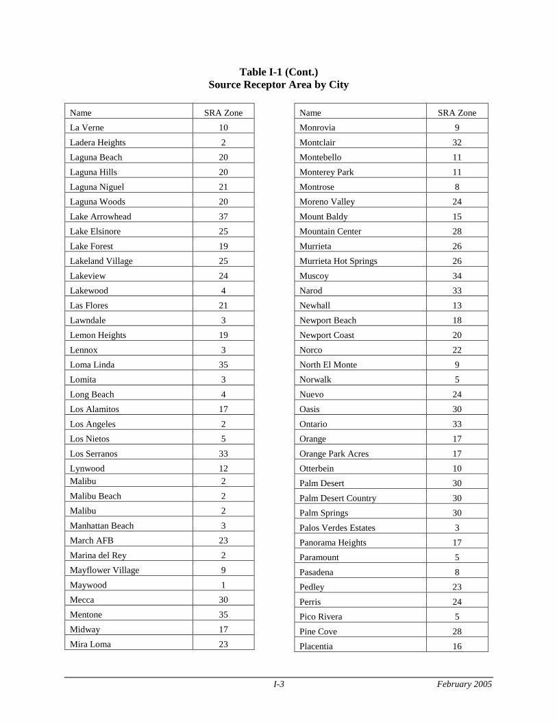
I-3 February 2005
Table I-1 (Cont.) Source Receptor Area by City
Name SRA Zone
La Verne 10
Ladera Heights 2
Laguna Beach 20
Laguna Hills 20
Laguna Niguel 21
Laguna Woods 20
Lake Arrowhead 37
Lake Elsinore 25
Lake Forest 19
Lakeland Village 25
Lakeview 24
Lakewood 4
Las Flores 21
Lawndale 3
Lemon Heights 19
Lennox 3
Loma Linda 35
Lomita 3
Long Beach 4
Los Alamitos 17
Los Angeles 2
Los Nietos 5
Los Serranos 33
Lynwood 12
Malibu 2
Malibu Beach 2
Malibu 2
Manhattan Beach 3
March AFB 23
Marina del Rey 2
Mayflower Village 9
Maywood 1
Mecca 30
Mentone 35
Midway 17
Mira Loma 23
Name SRA Zone
Monrovia 9
Montclair 32
Montebello 11
Monterey Park 11
Montrose 8
Moreno Valley 24
Mount Baldy 15
Mountain Center 28
Murrieta 26
Murrieta Hot Springs 26
Muscoy 34
Narod 33
Newhall 13
Newport Beach 18
Newport Coast 20
Norco 22
North El Monte 9
Norwalk 5
Nuevo 24
Oasis 30
Ontario 33
Orange 17
Orange Park Acres 17
Otterbein 10
Palm Desert 30
Palm Desert Country 30
Palm Springs 30
Palos Verdes Estates 3
Panorama Heights 17
Paramount 5
Pasadena 8
Pedley 23
Perris 24
Pico Rivera 5
Pine Cove 28
Placentia 16
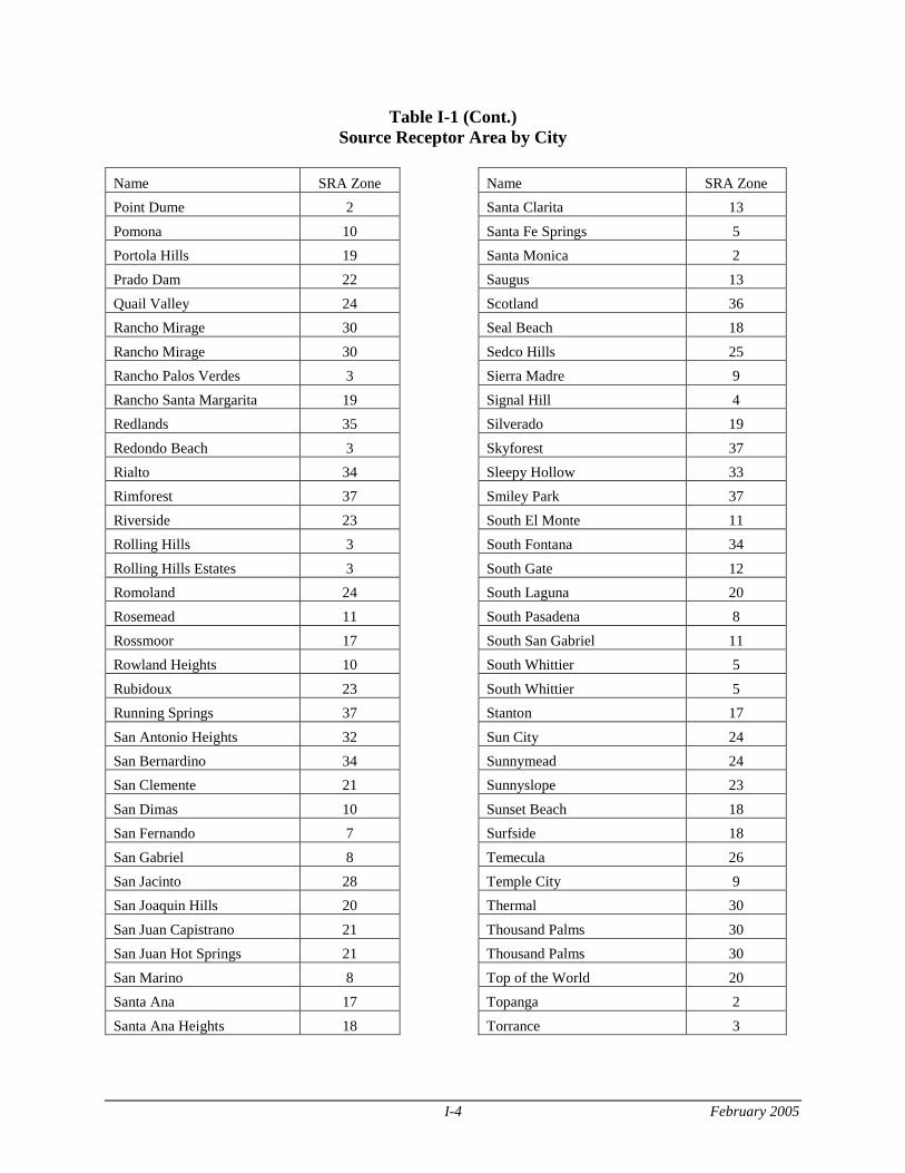
I-4 February 2005
Table I-1 (Cont.) Source Receptor Area by City
Name SRA Zone
Point Dume 2
Pomona 10
Portola Hills 19
Prado Dam 22
Quail Valley 24
Rancho Mirage 30
Rancho Mirage 30
Rancho Palos Verdes 3
Rancho Santa Margarita 19
Redlands 35
Redondo Beach 3
Rialto 34
Rimforest 37
Riverside 23
Rolling Hills 3
Rolling Hills Estates 3
Romoland 24
Rosemead 11
Rossmoor 17
Rowland Heights 10
Rubidoux 23
Running Springs 37
San Antonio Heights 32
San Bernardino 34
San Clemente 21
San Dimas 10
San Fernando 7
San Gabriel 8
San Jacinto 28
San Joaquin Hills 20
San Juan Capistrano 21
San Juan Hot Springs 21
San Marino 8
Santa Ana 17
Santa Ana Heights 18
Name SRA Zone
Santa Clarita 13
Santa Fe Springs 5
Santa Monica 2
Saugus 13
Scotland 36
Seal Beach 18
Sedco Hills 25
Sierra Madre 9
Signal Hill 4
Silverado 19
Skyforest 37
Sleepy Hollow 33
Smiley Park 37
South El Monte 11
South Fontana 34
South Gate 12
South Laguna 20
South Pasadena 8
South San Gabriel 11
South Whittier 5
South Whittier 5
Stanton 17
Sun City 24
Sunnymead 24
Sunnyslope 23
Sunset Beach 18
Surfside 18
Temecula 26
Temple City 9
Thermal 30
Thousand Palms 30
Thousand Palms 30
Top of the World 20
Topanga 2
Torrance 3
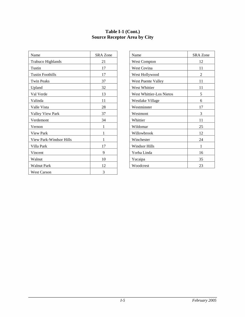
I-5 February 2005
Table I-1 (Cont.) Source Receptor Area by City
Name SRA Zone
Trabuco Highlands 21
Tustin 17
Tustin Foothills 17
Twin Peaks 37
Upland 32
Val Verde 13
Valinda 11
Valle Vista 28
Valley View Park 37
Verdemont 34
Vernon 1
View Park 1
View Park-Windsor Hills 1
Villa Park 17
Vincent 9
Walnut 10
Walnut Park 12
West Carson 3
Name SRA Zone
West Compton 12
West Covina 11
West Hollywood 2
West Puente Valley 11
West Whittier 11
West Whittier-Los Nietos 5
Westlake Village 6
Westminster 17
Westmont 3
Whittier 11
Wildomar 25
Willowbrook 12
Winchester 24
Windsor Hills 1
Yorba Linda 16
Yucaipa 35
Woodcrest 23
February 2005
A P P E N D I X J - E M I S S I O N E S T I M A T I O N M E T H O D O L O G Y
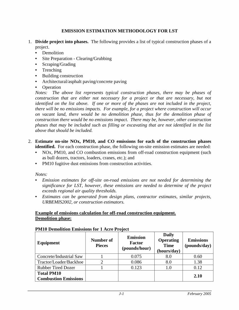
J-1 February 2005
EMISSION ESTIMATION METHODOLOGY FOR LST 1. Divide project into phases. The following provides a list of typical construction phases of a
project. • Demolition • Site Preparation - Clearing/Grubbing • Scraping/Grading • Trenching • Building construction • Architectural/asphalt paving/concrete paving • Operation Notes: The above list represents typical construction phases, there may be phases of construction that are either not necessary for a project or that are necessary, but not identified on the list above. If one or more of the phases are not included in the project, there will be no emissions impacts. For example, for a project where construction will occur on vacant land, there would be no demolition phase, thus for the demolition phase of construction there would be no emissions impact. There may be, however, other construction phases that may be included such as filling or excavating that are not identified in the list above that should be included.
2. Estimate on-site NOx, PM10, and CO emissions for each of the construction phases identified. For each construction phase, the following on-site emission estimates are needed: • NOx, PM10, and CO combustion emissions from off-road construction equipment (such
as bull dozers, tractors, loaders, cranes, etc.); and • PM10 fugitive dust emissions from construction activities.
Notes: • Emission estimates for off-site on-road emissions are not needed for determining the
significance for LST, however, these emissions are needed to determine of the project exceeds regional air quality thresholds.
• Estimates can be generated from design plans, contractor estimates, similar projects, URBEMIS2002, or construction estimators.
Example of emissions calculation for off-road construction equipment. Demolition phase: PM10 Demolition Emissions for 1 Acre Project
Equipment Number of Pieces
Emission Factor
(pounds/hour)
Daily Operating
Time (hours/day)
Emissions (pounds/day)
Concrete/Industrial Saw 1 0.075 8.0 0.60 Tractor/Loader/Backhoe 2 0.086 8.0 1.38 Rubber Tired Dozer 1 0.123 1.0 0.12 Total PM10 Combustion Emissions
2.10
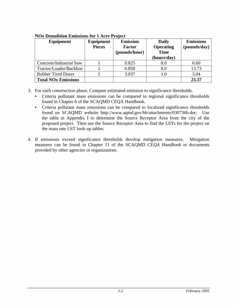
J-2 February 2005
NOx Demolition Emissions for 1 Acre Project
Equipment Equipment Pieces
Emission Factor
(pounds/hour)
Daily Operating
Time (hours/day)
Emissions (pounds/day)
Concrete/Industrial Saw 1 0.825 8.0 6.60 Tractor/Loader/Backhoe 2 0.858 8.0 13.73 Rubber Tired Dozer 1 3.037 1.0 3.04 Total NOx Emissions 23.37
3. For each construction phase, Compare estimated emission to significance thresholds.
• Criteria pollutant mass emissions can be compared to regional significance thresholds found in Chapter 6 of the SCAQMD CEQA Handbook.
• Criteria pollutant mass emissions can be compared to localized significance thresholds found on SCAQMD website http://www.aqmd.gov/hb/attachments/030736b.doc. Use the table in Appendix I to determine the Source Receptor Area from the city of the proposed project. Then use the Source Receptor Area to find the LSTs for the project on the mass rate LST look-up tables.
4. If emissions exceed significance thresholds develop mitigation measures. Mitigation
measures can be found in Chapter 11 of the SCAQMD CEQA Handbook or documents provided by other agencies or organizations.
February 2005
A P P E N D I X K - L I N E A R R E G R E S S I O N
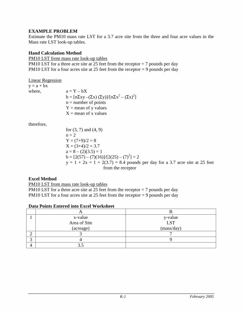
K-1 February 2005
EXAMPLE PROBLEM Estimate the PM10 mass rate LST for a 3.7 acre site from the three and four acre values in the Mass rate LST look-up tables.
Hand Calculation Method PM10 LST from mass rate look-up tables PM10 LST for a three acre site at 25 feet from the receptor = 7 pounds per day PM10 LST for a four acres site at 25 feet from the receptor = 9 pounds per day Linear Regession y = a + bx where, a = Y – bX b = [nΣxy –(Σx) (Σy)]/[nΣx2 – (Σx)2] n = number of points Y = mean of y values X = mean of x values therefore, for (3, 7) and (4, 9) n = 2 Y = (7+9)/2 = 8 X = (3+4)/2 = 3.7 a = 8 – (2)(3.5) = 1 b = [2(57) – (7)(16)]/[2(25) – (7)2] = 2 y = 1 + 2x = 1 + 2(3.7) = 8.4 pounds per day for a 3.7 acre site at 25 feet
from the receptor Excel Method PM10 LST from mass rate look-up tables PM10 LST for a three acre site at 25 feet from the receptor = 7 pounds per day PM10 LST for a four acres site at 25 feet from the receptor = 9 pounds per day Data Points Entered into Excel Worksheet A B 1 x-value
Area of Site (acreage)
y-value LST
(mass/day) 2 3 7 3 4 9 4 3.5
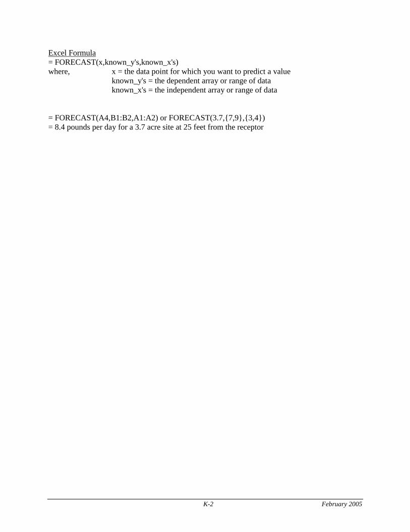
K-2 February 2005
Excel Formula = FORECAST(x,known_y's,known_x's) where, x = the data point for which you want to predict a value known_y's = the dependent array or range of data known_x's = the independent array or range of data = FORECAST(A4,B1:B2,A1:A2) or FORECAST(3.7,{7,9},{3,4}) = 8.4 pounds per day for a 3.7 acre site at 25 feet from the receptor
February 2005
A P P E N D I X L - 2 0 0 1 – 2 0 0 3 L O C A L I Z E S I G N I F I C A N C E T H R E S H O L D M A S S – R A T E L O O K – U P T A B L E S
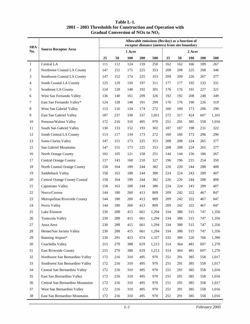
L-1 February 2005
Table L-1. 2001 – 2003 Thresholds for Construction and Operation with
Gradual Conversion of NOx to NO2
Allowable emissions (lbs/day) as a function of receptor distance (meters) from site boundary
1 Acre 2 Acre SRA No. Source Receptor Area
25 50 100 200 500 25 50 100 200 500
1 Central LA 111 112 124 159 250 162 162 166 189 267
2 Northwest Coastal LA County 147 151 175 225 353 208 208 225 268 346
3 Southwest Coastal LA County 147 152 174 225 353 209 209 226 267 377
4 South Coastal LA County 125 129 150 197 311 177 177 192 233 331
5 Southeast LA County 124 128 148 192 301 176 176 191 227 321
6 West San Fernando Valley 136 140 161 209 326 192 192 208 248 349
7 East San Fernando Valley* 124 128 148 191 299 176 176 190 226 319
8 West San Gabriel Valley 113 116 134 174 272 160 160 173 206 290
9 East San Gabriel Valley 187 237 338 537 1,051 272 317 424 607 1,101
10 Pomona/Walnut Valley 172 216 310 495 970 251 291 385 558 1,016
11 South San Gabriel Valley 130 133 152 193 302 187 187 198 231 322
12 South Central LA County 113 117 134 173 272 160 160 173 206 290
13 Santa Clarita Valley 147 151 173 225 353 208 208 224 265 377
15 San Gabriel Mountains 147 151 173 225 353 208 208 224 265 377
16 North Orange County 102 105 121 158 251 144 144 156 186 267
17 Central Orange County 137 143 168 210 327 196 196 215 254 350
18 North Coastal Orange County 158 164 189 244 382 226 226 244 288 408
19 Saddleback Valley 158 163 188 244 380 224 224 243 289 407
20 Central Orange County Coastal 158 164 189 244 382 226 226 244 288 408
21 Capistrano Valley 158 163 188 244 380 224 224 243 289 407
22 Norco/Corona 144 180 260 413 809 209 242 322 467 847
23 Metropolitan Riverside County 144 180 260 413 809 209 242 322 467 847
24 Perris Valley 144 180 260 413 809 209 242 322 467 847
25 Lake Elsinore 230 288 415 661 1,294 334 388 515 747 1,356
26 Temecula Valley 230 288 415 661 1,294 334 388 515 747 1,356
27 Anza Area 230 288 415 661 1,294 334 388 515 747 1,356
28 Hemet/San Jacinto Valley 230 288 415 661 1,294 334 388 515 747 1,356
29 Banning Airport* 230 291 423 674 1,327 335 389 520 766 1,390
30 Coachella Valley 215 270 388 619 1,213 314 364 481 697 1,270
31 East Riverside County 215 270 388 619 1,213 314 364 481 697 1,270
32 Northwest San Bernardino Valley 172 216 310 495 970 251 291 385 558 1,017
33 Southwest San Bernardino Valley 172 216 310 495 970 251 291 385 558 1,017
34 Central San Bernardino Valley 172 216 310 495 970 251 291 385 558 1,016
35 East San Bernardino Valley 172 216 310 495 970 251 291 385 558 1,016
36 Central San Bernardino Mountains 172 216 310 495 970 251 291 385 558 1,017
37 West San Bernardino Valley 172 216 310 495 970 251 291 385 558 1,016
38 East San Bernardino Mountains 172 216 310 495 970 251 291 385 558 1,016
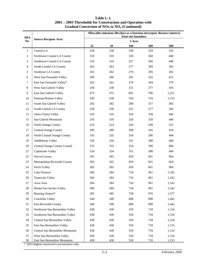
L-2 February 2005
Table L-1. 2001 – 2003 Thresholds for Construction and Operation with
Gradual Conversion of NOx to NO2 (Continued)
Allowable emissions (lbs/day) as a function ofreceptor distance (meters) from site boundary
5 Acre SRA No. Source Receptor Area
25 50 100 200 500
1 Central LA 238 238 249 259 316
2 Northwest Coastal LA County 310 310 326 360 448
3 Southwest Coastal LA County 310 310 327 360 448
4 South Coastal LA County 263 263 277 309 392
5 Southeast LA County 262 262 276 305 382
6 West San Fernando Valley 286 286 301 332 415
7 East San Fernando Valley* 262 262 276 304 379
8 West San Gabriel Valley 238 238 251 277 345
9 East San Gabriel Valley 475 475 601 786 1,251
10 Pomona/Walnut Valley 438 438 550 718 1,153
11 South San Gabriel Valley 282 282 289 317 383
12 South Central LA County 238 238 251 277 345
13 Santa Clarita Valley 310 310 326 358 446
15 San Gabriel Mountains 310 310 326 358 446
16 North Orange County 214 214 226 249 315
17 Central Orange County 289 289 308 345 418
18 North Coastal Orange County 335 335 354 390 484
19 Saddleback Valley 334 334 351 388 484
20 Central Orange County Coastal 335 335 354 390 484
21 Capistrano Valley 334 334 351 388 484
22 Norco/Corona 365 365 459 601 964
23 Metropolitan Riverside County 365 365 459 601 964
24 Perris Valley 365 365 459 601 964
25 Lake Elsinore 584 584 734 961 1,542
26 Temecula Valley 584 584 734 961 1,542
27 Anza Area 584 584 734 961 1,542
28 Hemet/San Jacinto Valley 584 584 734 961 1,542
29 Banning Airport* 585 585 738 976 1,577
30 Coachella Valley 548 548 688 898 1,442
31 East Riverside County 548 548 688 898 1,442
32 Northwest San Bernardino Valley 438 438 550 718 1,154
33 Southwest San Bernardino Valley 438 438 550 718 1,154
34 Central San Bernardino Valley 438 438 550 718 1,154
35 East San Bernardino Valley 438 438 550 718 1,153
36 Central San Bernardino Mountains 438 438 550 718 1,154
37 West San Bernardino Valley 438 438 550 718 1,154
38 East San Bernardino Mountains 438 438 550 718 1,153 * 2003 highest monitored concentration only.
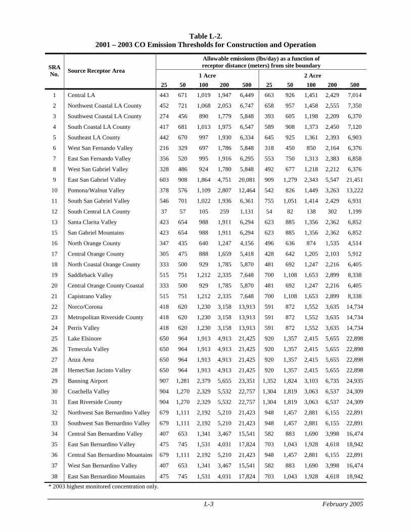
L-3 February 2005
Table L-2. 2001 – 2003 CO Emission Thresholds for Construction and Operation
Allowable emissions (lbs/day) as a function of receptor distance (meters) from site boundary
1 Acre 2 Acre SRA No. Source Receptor Area
25 50 100 200 500 25 50 100 200 500
1 Central LA 443 671 1,019 1,947 6,449 663 926 1,451 2,429 7,014
2 Northwest Coastal LA County 452 721 1,068 2,053 6,747 658 957 1,458 2,555 7,350
3 Southwest Coastal LA County 274 456 890 1,779 5,848 393 605 1,198 2,209 6,370
4 South Coastal LA County 417 681 1,013 1,975 6,547 589 908 1,373 2,450 7,120
5 Southeast LA County 442 670 997 1,930 6,334 645 925 1,361 2,393 6,903
6 West San Fernando Valley 216 329 697 1,786 5,848 318 450 850 2,164 6,376
7 East San Fernando Valley 356 520 995 1,916 6,295 553 750 1,313 2,383 6,858
8 West San Gabriel Valley 328 486 924 1,780 5,848 492 677 1,218 2,212 6,376
9 East San Gabriel Valley 603 908 1,864 4,751 20,081 909 1,279 2,343 5,547 21,451
10 Pomona/Walnut Valley 378 576 1,109 2,807 12,464 542 826 1,449 3,263 13,222
11 South San Gabriel Valley 546 701 1,022 1,936 6,361 755 1,051 1,414 2,429 6,931
12 South Central LA County 37 57 105 259 1,131 54 82 138 302 1,199
13 Santa Clarita Valley 423 654 988 1,911 6,294 623 885 1,356 2,362 6,852
15 San Gabriel Mountains 423 654 988 1,911 6,294 623 885 1,356 2,362 6,852
16 North Orange County 347 435 640 1,247 4,156 496 636 874 1,535 4,514
17 Central Orange County 305 475 888 1,659 5,418 428 642 1,205 2,103 5,912
18 North Coastal Orange County 333 500 929 1,785 5,870 481 692 1,247 2,216 6,405
19 Saddleback Valley 515 751 1,212 2,335 7,648 700 1,108 1,653 2,899 8,338
20 Central Orange County Coastal 333 500 929 1,785 5,870 481 692 1,247 2,216 6,405
21 Capistrano Valley 515 751 1,212 2,335 7,648 700 1,108 1,653 2,899 8,338
22 Norco/Corona 418 620 1,230 3,158 13,913 591 872 1,552 3,635 14,734
23 Metropolitan Riverside County 418 620 1,230 3,158 13,913 591 872 1,552 3,635 14,734
24 Perris Valley 418 620 1,230 3,158 13,913 591 872 1,552 3,635 14,734
25 Lake Elsinore 650 964 1,913 4,913 21,425 920 1,357 2,415 5,655 22,898
26 Temecula Valley 650 964 1,913 4,913 21,425 920 1,357 2,415 5,655 22,898
27 Anza Area 650 964 1,913 4,913 21,425 920 1,357 2,415 5,655 22,898
28 Hemet/San Jacinto Valley 650 964 1,913 4,913 21,425 920 1,357 2,415 5,655 22,898
29 Banning Airport 907 1,281 2,379 5,655 23,351 1,352 1,824 3,103 6,735 24,935
30 Coachella Valley 904 1,270 2,329 5,532 22,757 1,304 1,819 3,063 6,537 24,309
31 East Riverside County 904 1,270 2,329 5,532 22,757 1,304 1,819 3,063 6,537 24,309
32 Northwest San Bernardino Valley 679 1,111 2,192 5,210 21,423 948 1,457 2,881 6,155 22,891
33 Southwest San Bernardino Valley 679 1,111 2,192 5,210 21,423 948 1,457 2,881 6,155 22,891
34 Central San Bernardino Valley 407 653 1,341 3,467 15,541 582 883 1,690 3,998 16,474
35 East San Bernardino Valley 475 745 1,531 4,031 17,824 703 1,043 1,928 4,618 18,942
36 Central San Bernardino Mountains 679 1,111 2,192 5,210 21,423 948 1,457 2,881 6,155 22,891
37 West San Bernardino Valley 407 653 1,341 3,467 15,541 582 883 1,690 3,998 16,474
38 East San Bernardino Mountains 475 745 1,531 4,031 17,824 703 1,043 1,928 4,618 18,942
* 2003 highest monitored concentration only.
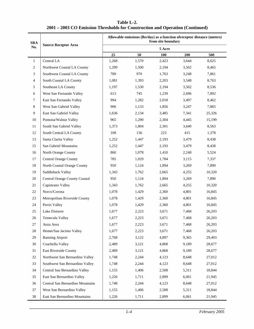
L-4 February 2005
Table L-2. 2001 – 2003 CO Emission Thresholds for Construction and Operation (Continued)
Allowable emissions (lbs/day) as a function ofreceptor distance (meters) from site boundary
5 Acre
SRA No. Source Receptor Area
25 50 100 200 500
1 Central LA 1,268 1,570 2,423 3,644 8,625
2 Northwest Coastal LA County 1,299 1,500 2,194 3,502 8,465
3 Southwest Coastal LA County 789 970 1,763 3,248 7,861
4 South Coastal LA County 1,081 1,393 2,203 3,548 8,763
5 Southeast LA County 1,197 1,530 2,194 3,502 8,536
6 West San Fernando Valley 613 745 1,239 2,696 7,892
7 East San Fernando Valley 994 1,282 2,018 3,497 8,462
8 West San Gabriel Valley 906 1,133 1,856 3,247 7,865
9 East San Gabriel Valley 1,636 2,134 3,485 7,341 25,326
10 Pomona/Walnut Valley 965 1,290 2,304 4,445 15,199
11 South San Gabriel Valley 1,373 1,804 2,301 3,640 8,563
12 South Central LA County 108 136 223 415 1,378
13 Santa Clarita Valley 1,252 1,447 2,193 3,479 8,438
15 San Gabriel Mountains 1,252 1,447 2,193 3,479 8,438
16 North Orange County 860 1,078 1,410 2,248 5,524
17 Central Orange County 785 1,029 1,784 3,115 7,337
18 North Coastal Orange County 950 1,124 1,894 3,269 7,890
19 Saddleback Valley 1,343 1,762 2,665 4,255 10,320
20 Central Orange County Coastal 950 1,124 1,894 3,269 7,890
21 Capistrano Valley 1,343 1,762 2,665 4,255 10,320
22 Norco/Corona 1,078 1,429 2,360 4,801 16,845
23 Metropolitan Riverside County 1,078 1,429 2,360 4,801 16,845
24 Perris Valley 1,078 1,429 2,360 4,801 16,845
25 Lake Elsinore 1,677 2,223 3,671 7,468 26,203
26 Temecula Valley 1,677 2,223 3,671 7,468 26,203
27 Anza Area 1,677 2,223 3,671 7,468 26,203
28 Hemet/San Jacinto Valley 1,677 2,223 3,671 7,468 26,203
29 Banning Airport 2,768 3,122 4,897 9,365 29,403
30 Coachella Valley 2,489 3,121 4,868 9,189 28,677
31 East Riverside County 2,489 3,121 4,868 9,189 28,677
32 Northwest San Bernardino Valley 1,748 2,244 4,123 8,648 27,012
33 Southwest San Bernardino Valley 1,748 2,244 4,123 8,648 27,012
34 Central San Bernardino Valley 1,155 1,406 2,508 5,311 18,844
35 East San Bernardino Valley 1,226 1,711 2,899 6,061 21,945
36 Central San Bernardino Mountains 1,748 2,244 4,123 8,648 27,012
37 West San Bernardino Valley 1,155 1,406 2,508 5,311 18,844
38 East San Bernardino Mountains 1,226 1,711 2,899 6,061 21,945
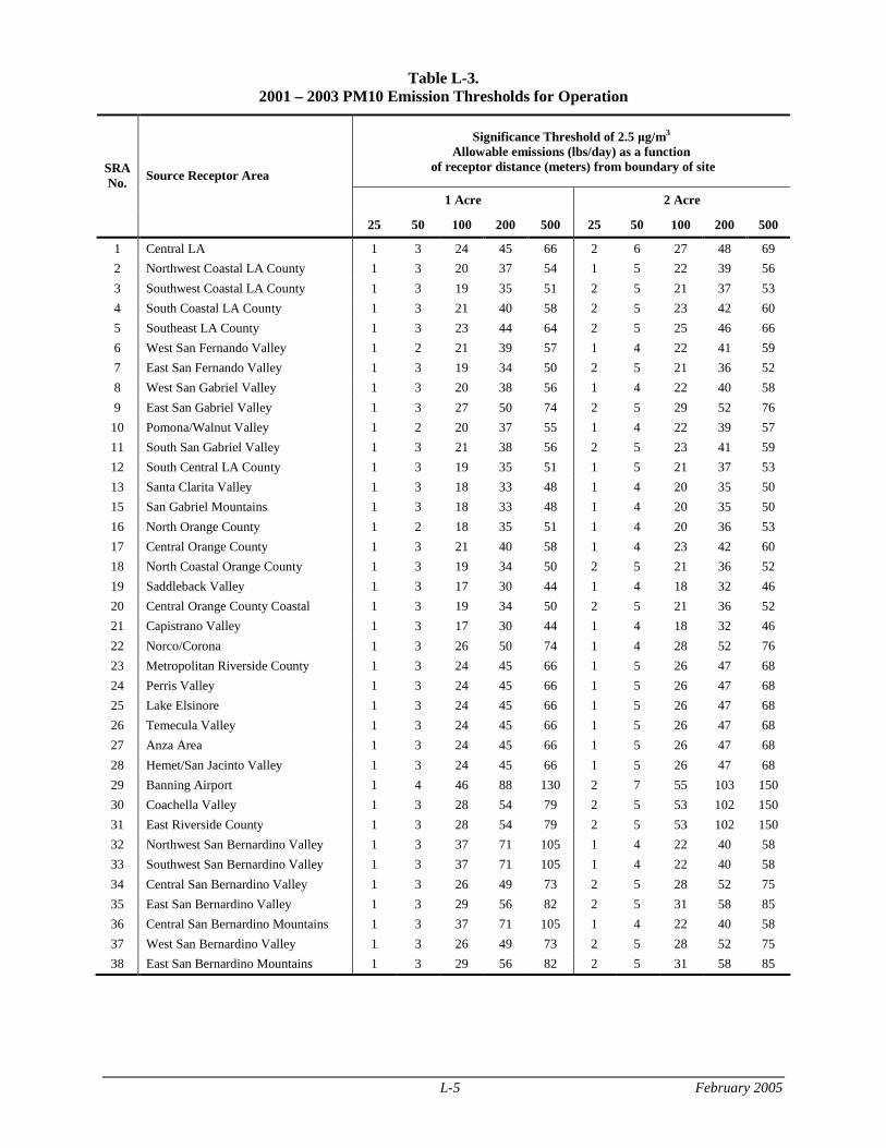
L-5 February 2005
Table L-3. 2001 – 2003 PM10 Emission Thresholds for Operation
Significance Threshold of 2.5 �g/m3 Allowable emissions (lbs/day) as a function
of receptor distance (meters) from boundary of site
1 Acre 2 Acre
SRA No. Source Receptor Area
25 50 100 200 500 25 50 100 200 500
1 Central LA 1 3 24 45 66 2 6 27 48 69
2 Northwest Coastal LA County 1 3 20 37 54 1 5 22 39 56
3 Southwest Coastal LA County 1 3 19 35 51 2 5 21 37 53
4 South Coastal LA County 1 3 21 40 58 2 5 23 42 60
5 Southeast LA County 1 3 23 44 64 2 5 25 46 66
6 West San Fernando Valley 1 2 21 39 57 1 4 22 41 59
7 East San Fernando Valley 1 3 19 34 50 2 5 21 36 52
8 West San Gabriel Valley 1 3 20 38 56 1 4 22 40 58
9 East San Gabriel Valley 1 3 27 50 74 2 5 29 52 76
10 Pomona/Walnut Valley 1 2 20 37 55 1 4 22 39 57
11 South San Gabriel Valley 1 3 21 38 56 2 5 23 41 59
12 South Central LA County 1 3 19 35 51 1 5 21 37 53
13 Santa Clarita Valley 1 3 18 33 48 1 4 20 35 50
15 San Gabriel Mountains 1 3 18 33 48 1 4 20 35 50
16 North Orange County 1 2 18 35 51 1 4 20 36 53
17 Central Orange County 1 3 21 40 58 1 4 23 42 60
18 North Coastal Orange County 1 3 19 34 50 2 5 21 36 52
19 Saddleback Valley 1 3 17 30 44 1 4 18 32 46
20 Central Orange County Coastal 1 3 19 34 50 2 5 21 36 52
21 Capistrano Valley 1 3 17 30 44 1 4 18 32 46
22 Norco/Corona 1 3 26 50 74 1 4 28 52 76
23 Metropolitan Riverside County 1 3 24 45 66 1 5 26 47 68
24 Perris Valley 1 3 24 45 66 1 5 26 47 68
25 Lake Elsinore 1 3 24 45 66 1 5 26 47 68
26 Temecula Valley 1 3 24 45 66 1 5 26 47 68
27 Anza Area 1 3 24 45 66 1 5 26 47 68
28 Hemet/San Jacinto Valley 1 3 24 45 66 1 5 26 47 68
29 Banning Airport 1 4 46 88 130 2 7 55 103 150
30 Coachella Valley 1 3 28 54 79 2 5 53 102 150
31 East Riverside County 1 3 28 54 79 2 5 53 102 150
32 Northwest San Bernardino Valley 1 3 37 71 105 1 4 22 40 58
33 Southwest San Bernardino Valley 1 3 37 71 105 1 4 22 40 58
34 Central San Bernardino Valley 1 3 26 49 73 2 5 28 52 75
35 East San Bernardino Valley 1 3 29 56 82 2 5 31 58 85
36 Central San Bernardino Mountains 1 3 37 71 105 1 4 22 40 58
37 West San Bernardino Valley 1 3 26 49 73 2 5 28 52 75
38 East San Bernardino Mountains 1 3 29 56 82 2 5 31 58 85
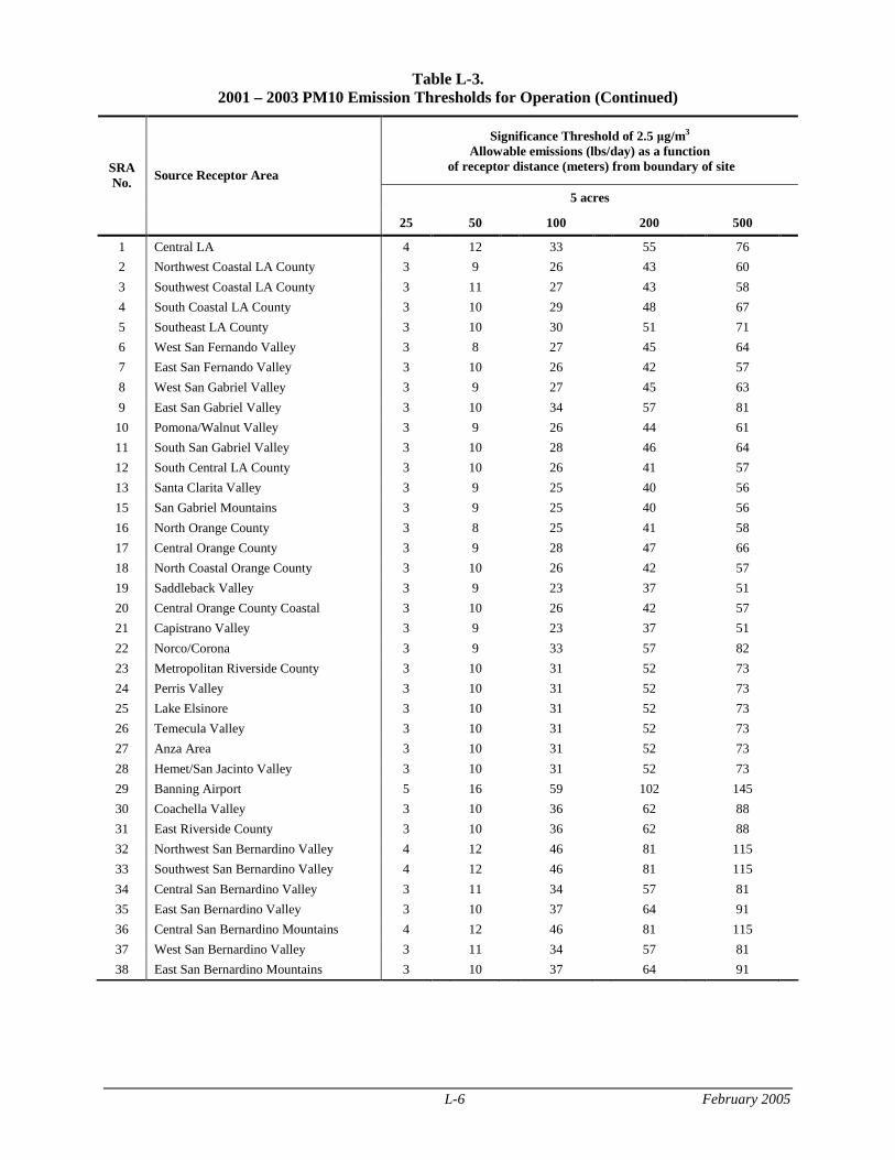
L-6 February 2005
Table L-3. 2001 – 2003 PM10 Emission Thresholds for Operation (Continued)
Significance Threshold of 2.5 �g/m3 Allowable emissions (lbs/day) as a function
of receptor distance (meters) from boundary of site
5 acres
SRA No. Source Receptor Area
25 50 100 200 500
1 Central LA 4 12 33 55 76
2 Northwest Coastal LA County 3 9 26 43 60
3 Southwest Coastal LA County 3 11 27 43 58
4 South Coastal LA County 3 10 29 48 67
5 Southeast LA County 3 10 30 51 71
6 West San Fernando Valley 3 8 27 45 64
7 East San Fernando Valley 3 10 26 42 57
8 West San Gabriel Valley 3 9 27 45 63
9 East San Gabriel Valley 3 10 34 57 81
10 Pomona/Walnut Valley 3 9 26 44 61
11 South San Gabriel Valley 3 10 28 46 64
12 South Central LA County 3 10 26 41 57
13 Santa Clarita Valley 3 9 25 40 56
15 San Gabriel Mountains 3 9 25 40 56
16 North Orange County 3 8 25 41 58
17 Central Orange County 3 9 28 47 66
18 North Coastal Orange County 3 10 26 42 57
19 Saddleback Valley 3 9 23 37 51
20 Central Orange County Coastal 3 10 26 42 57
21 Capistrano Valley 3 9 23 37 51
22 Norco/Corona 3 9 33 57 82
23 Metropolitan Riverside County 3 10 31 52 73
24 Perris Valley 3 10 31 52 73
25 Lake Elsinore 3 10 31 52 73
26 Temecula Valley 3 10 31 52 73
27 Anza Area 3 10 31 52 73
28 Hemet/San Jacinto Valley 3 10 31 52 73
29 Banning Airport 5 16 59 102 145
30 Coachella Valley 3 10 36 62 88
31 East Riverside County 3 10 36 62 88
32 Northwest San Bernardino Valley 4 12 46 81 115
33 Southwest San Bernardino Valley 4 12 46 81 115
34 Central San Bernardino Valley 3 11 34 57 81
35 East San Bernardino Valley 3 10 37 64 91
36 Central San Bernardino Mountains 4 12 46 81 115
37 West San Bernardino Valley 3 11 34 57 81
38 East San Bernardino Mountains 3 10 37 64 91
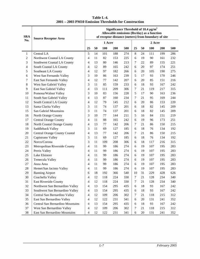
L-7 February 2005
Table L-4. 2001 – 2003 PM10 Emission Thresholds for Construction
Significance Threshold of 10.4 �g/m3 Allowable emissions (lbs/day) as a function
of receptor distance (meters) from boundary of site
1 Acre 2 Acre
SRA No. Source Receptor Area
25 50 100 200 500 25 50 100 200 500
1 Central LA 5 14 101 188 274 8 24 111 199 286 2 Northwest Coastal LA County 4 11 82 153 225 6 19 90 161 232 3 Southwest Coastal LA County 4 13 80 146 213 7 22 89 155 221 4 South Coastal LA County 4 12 89 165 242 6 20 97 174 251 5 Southeast LA County 4 12 97 182 266 6 20 105 190 275 6 West San Fernando Valley 3 10 86 163 239 5 17 93 170 246 7 East San Fernando Valley 4 12 77 142 207 6 20 85 151 216 8 West San Gabriel Valley 3 11 85 159 233 6 18 93 167 242 9 East San Gabriel Valley 4 13 111 209 306 7 21 119 217 315 10 Pomona/Walnut Valley 3 10 83 156 228 5 17 90 163 236 11 South San Gabriel Valley 4 13 87 160 234 7 21 95 169 244 12 South Central LA County 4 12 79 145 212 6 20 86 153 220 13 Santa Clarita Valley 3 11 74 137 201 6 18 82 145 209 15 San Gabriel Mountains 3 11 74 137 201 6 18 82 145 209 16 North Orange County 3 10 77 144 211 5 16 84 151 219 17 Central Orange County 4 11 88 165 242 6 19 96 173 251 18 North Coastal Orange County 4 13 77 142 206 7 21 86 150 215 19 Saddleback Valley 3 11 69 127 185 6 18 76 134 192 20 Central Orange County Coastal 4 13 77 142 206 7 21 86 150 215 21 Capistrano Valley 3 11 69 127 185 6 18 76 134 192 22 Norco/Corona 3 11 109 208 306 6 18 117 216 315 23 Metropolitan Riverside County 4 11 99 186 274 6 19 107 195 283 24 Perris Valley 4 11 99 186 274 6 19 107 195 283 25 Lake Elsinore 4 11 99 186 274 6 19 107 195 283 26 Temecula Valley 4 11 99 186 274 6 19 107 195 283 27 Anza Area 4 11 99 186 274 6 19 107 195 283 28 Hemet/San Jacinto Valley 4 11 99 186 274 6 19 107 195 283 29 Banning Airport 6 18 192 366 540 10 31 229 428 626 30 Coachella Valley 4 12 118 224 330 7 21 128 234 340 31 East Riverside County 4 12 118 224 330 7 21 128 234 340 32 Northwest San Bernardino Valley 4 13 154 295 435 6 18 93 167 242 33 Southwest San Bernardino Valley 4 13 154 295 435 6 18 93 167 242 34 Central San Bernardino Valley 4 12 109 206 302 7 21 118 215 312 35 East San Bernardino Valley 4 12 122 231 341 6 20 131 241 352 36 Central San Bernardino Mountains 4 13 154 295 435 6 18 93 167 242 37 West San Bernardino Valley 4 12 109 206 302 7 21 118 215 312 38 East San Bernardino Mountains 4 12 122 231 341 6 20 131 241 352
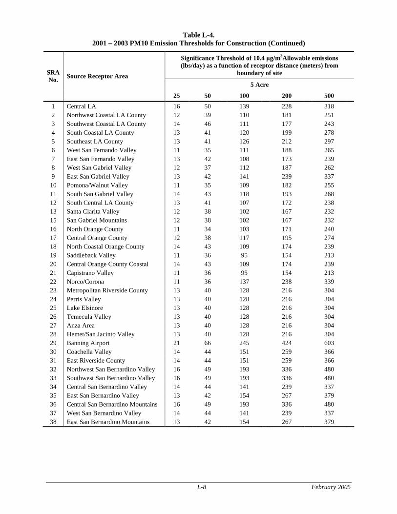
L-8 February 2005
Table L-4. 2001 – 2003 PM10 Emission Thresholds for Construction (Continued)
Significance Threshold of 10.4 �g/m3Allowable emissions (lbs/day) as a function of receptor distance (meters) from
boundary of site
5 Acre
SRA No. Source Receptor Area
25 50 100 200 500
1 Central LA 16 50 139 228 318 2 Northwest Coastal LA County 12 39 110 181 251 3 Southwest Coastal LA County 14 46 111 177 243 4 South Coastal LA County 13 41 120 199 278 5 Southeast LA County 13 41 126 212 297 6 West San Fernando Valley 11 35 111 188 265 7 East San Fernando Valley 13 42 108 173 239 8 West San Gabriel Valley 12 37 112 187 262 9 East San Gabriel Valley 13 42 141 239 337 10 Pomona/Walnut Valley 11 35 109 182 255 11 South San Gabriel Valley 14 43 118 193 268 12 South Central LA County 13 41 107 172 238 13 Santa Clarita Valley 12 38 102 167 232 15 San Gabriel Mountains 12 38 102 167 232 16 North Orange County 11 34 103 171 240 17 Central Orange County 12 38 117 195 274 18 North Coastal Orange County 14 43 109 174 239 19 Saddleback Valley 11 36 95 154 213 20 Central Orange County Coastal 14 43 109 174 239 21 Capistrano Valley 11 36 95 154 213 22 Norco/Corona 11 36 137 238 339 23 Metropolitan Riverside County 13 40 128 216 304 24 Perris Valley 13 40 128 216 304 25 Lake Elsinore 13 40 128 216 304 26 Temecula Valley 13 40 128 216 304 27 Anza Area 13 40 128 216 304 28 Hemet/San Jacinto Valley 13 40 128 216 304 29 Banning Airport 21 66 245 424 603 30 Coachella Valley 14 44 151 259 366 31 East Riverside County 14 44 151 259 366 32 Northwest San Bernardino Valley 16 49 193 336 480 33 Southwest San Bernardino Valley 16 49 193 336 480 34 Central San Bernardino Valley 14 44 141 239 337 35 East San Bernardino Valley 13 42 154 267 379 36 Central San Bernardino Mountains 16 49 193 336 480 37 West San Bernardino Valley 14 44 141 239 337 38 East San Bernardino Mountains 13 42 154 267 379