Financial Education and the Debt Behavior of the Young

This paper presents preliminary findings and is being distributed to economists

and other interested readers solely to stimulate discussion and elicit comments.

The views expressed in this paper are those of the authors and do not necessarily

reflect the position of the Federal Reserve Bank of New York or the Federal

Reserve System. Any errors or omissions are the responsibility of the authors.

Federal Reserve Bank of New York

Staff Reports

Financial Education and the Debt

Behavior of the Young

Meta Brown

John Grigsby

Wilbert van der Klaauw

Jaya Wen

Basit Zafar

Staff Report No. 634

September 2013

Revised September 2015

Financial Education and the Debt Behavior of the Young

Meta Brown, John Grigsby, Wilbert van der Klaauw, Jaya Wen, and Basit Zafar

Federal Reserve Bank of New York Staff Reports, no. 634

September 2013; revised September 2015

JEL classification: A20, D12, D14

Abstract

Young Americans are heavily reliant on debt and have clear financial literacy shortcomings, yet

evidence on the relationship between financial education and youths’ subsequent debt behavior

remains both limited and mixed. In this paper, we study the effects of exposure to financial

training on debt outcomes in early adulthood among a large and representative sample of young

Americans. Variation in exposure to financial training comes from statewide changes in high

school graduation requirements regarding financial literacy, economics, and mathematics that

were mandated in the late 1990s and 2000s. The FRBNY Consumer Credit Panel provides debt

outcomes based on quarterly Equifax credit reports from 1999 to 2014. Our analysis, based on a

flexible event study approach, reveals significant effects of quantitative training on debt-related

outcomes of youth. We find that exposure to math and financial literacy education modestly

decreases the incidence of adverse outcomes—such as delinquency and collections—and both

reduces the likelihood of youth carrying non-student debt and increases reliance on student debt.

All but the student debt effects tend to fade out with age. On the other hand, economic education

leads to an increase in the likelihood of adverse debt outcomes, and, relatedly, to a decline in

youths’ average risk scores. The effects are observed to accumulate as the borrower ages. Our

results suggest that financial education programs, increasingly promoted by policymakers, do

have significant impacts on the financial decision-making of youth, but their impacts may depend

on the content of the programs.

Key words: financial literacy, debt

_________________

Brown, van der Klaauw, Zafar: Federal Reserve Bank of New York (e-mail:

[email protected], [email protected], [email protected]). Grigsby:

University of Chicago (e-mail: [email protected]). Wen: Yale University (e-mail:

[email protected]). The authors would like to thank Zachary Bleemer and Michael Stewart

for invaluable research assistance, and Brian Bucks, Chris Carroll, Rajeev Darolia, Tullio

Jappelli, Henry Korytkowski, David Laibson, Maria Luengo-Prado, Silvia Magri, Olivia Mitchell,

Dekuwmini Mornah, Shannon Mudd, Anna Paulson, Max Schmeiser, Kartini Shastry, Joseph

Tracy, Didem Tüzemen, Carly Urban, Jonathan Willis, and seminar and conference participants

at the American Economic Association meetings, the Association for Education Finance and

Policy meetings, the Eastern Economic Association meetings, the ECB 2013 Conference on

Household Finance and Consumption, the 2014 NBER Summer Institute Children’s Workshop,

the 2015 European Conference on Household Finance, the Federal Reserve Banks of Kansas

City, New York, and Philadelphia, and the University of Michigan 2013 Aspen Conference on

Economic Decision-Making for comments. The views expressed in this paper are those of the

authors and do not necessarily reflect the position of the Federal Reserve Bank of New York or

the Federal Reserve System.

1

Young adults in the US are heavily reliant on debt, and their level of financial literacy is low.

Seventy-nine percent of 25-year-olds in the FRBNY Consumer Credit Panel (CCP) in 2012 held

consumer debt. The average debt balance among all 2012 CCP 25-year-olds was $22,911; similar

evidence on youth debt can be found in the 2010 SCF (Bricker et al., 2012). Despite this extensive

interaction with lending markets, a majority of high school and college students fail basic financial

literacy tests (Hastings, Madrian, and Skimmyhorn, 2013; Markow and Bagnaschi, 2005; Shim et al.,

2010). The low financial literacy rates among US youth and an effective delinquency rate of over 30% on

student loans for young borrowers in repayment (Brown et al., 2013a), along with the well-established

correlation between financial literacy and financial well-being, which we discuss later in the paper, has

prompted policy-makers and the media to push for more financial education.1 However, evidence of the

causal effect of financial training on debt outcomes for the young is based largely on field and natural

experiments of modest scale, and is, at best, mixed (see Fernandes, Lynch, and Netemeyer, 2014).

Our analysis addresses the question of the effectiveness of financial education by analyzing large-

scale changes in financial training exposure in a two percent sample of young Americans, and tracking

their debt outcomes over the decade immediately following the high school training. Given weak prior

evidence, we attempt to identify meaningful effects of financial training where we think they are most

likely to exist. We look for effects of very recent changes in financial training, which involve large

increases in required classroom hours and apply to millions of US students, and we look for these effects

in the years immediately following the training, in debt decisions that are relevant to most of the treated

population. Failure to find effects of financial training in this context could, following Fernandes et al.

(forthcoming), both unite and reinforce the findings of several smaller and disparate field studies. On the

other hand, evidence of meaningful effects of financial training in this context could derive from some or

all of a number of adjustments to the methodology. The technology of financial training may have

1 See, for example, Ferguson (2012) and Surowiecki (2010). Jack Lew, the Treasury Secretary, recently said: "In today’s economy, it is also essential for Americans to develop basic financial knowledge and learn how to navigate a complex financial system. We need to make sure young people can make smart decisions about what financial products to use. That young people can plan and save for the long term while managing expenses and debt in the short-term." (Treasury Department, 2013).

2

improved over recent decades. Effects may appear only following very intensive interventions, at earlier

ages only, or only in a much larger population. Finally, it may be necessary to track outcomes at very

young ages, shortly after training occurs, and in debt choices that are relevant to the majority of the

treated population.

For this purpose, we use variation in financial education – more specifically, financial literacy,

economics, and mathematics – graduation requirements mandated by state-level high school curricula

over the late 1990s and 2000s, in combination with detailed consumer liability data from the CCP. The

CCP isan ongoing quarterly panel on consumer debts comprising a five percent sample of U.S. credit

reports from Equifax, one of three major national credit reporting agencies.

Our identification strategy exploits variation in the timing of enactment of financial education

reforms in high school curricula across as well as within states. In 1999, ten states required high school

enrollment in economics courses, a number which doubled to 20 by 2012. Similarly, only one out of 50

states required a financial literacy course for graduation in 1999; by 2012, this number had increased to

17. And, though every state (except one) had some math graduation requirement in place at the start of

our time period, 19 states revised their standards upward by at least a full year between 1999 and 2012.

Our baseline empirical strategy, which employs fully flexible time trends for each state, and fully flexible

time trends for each cohort, in addition to a separate linear cohort trend for each state and a rich set of

local time-varying controls, uses these staggered policy changes to identify the causal impact of financial

education on debt-related outcomes of youth. In particular, we do not assume common time trends

across states, an assumption which has been shown to be problematic in the context of studies

that use changes in compulsory schooling laws (Stephens and Yang, 2014). That is, our empirical

specification directly controls for the possibility that states that implement financial training mandates

may have pre-existing trends that differ from those that do not, and that trends in the outcomes across

different birth cohorts may differ. Conditional on this extensive set of controls, our identifying

assumption hinges on states’ implementation of these reforms being uncorrelated with those omitted

3

determinants of financial outcomes that vary non-linearly from cohort to cohort within a state, and are not

shared either by all young residents of a given state in the current year or by all members of a given U.S.

cohort in the current year.

The empirical analysis reveals that exposure to financial and quantitative education has

significant, if moderate, impacts on the debt-related outcomes of 19 to 29 year olds. Additional

mathematics training leads to improved creditworthiness (as measured by the Equifax risk score, which is

similar to the FICO score), and decreases adverse outcomes such as accounts in collection. It also leads to

significant positive impacts on the propensity to hold student debt and on student debt balances. Math

education, however, has no impact on the extensive margin, that is, the likelihood of having a credit

report. Impacts of math education seem to fade out over time in early adulthood. The exception is student

borrowing, which accumulates as the borrower ages.

Financial literacy exposure increases the prevalence of credit reports in this age group. Since

having older credit accounts typically increases credit scores (Federal Reserve Bank of Philadelphia,

2012), this suggests improved understanding of the value of credit history. Along the intensive margin,

financial literacy training leads to a modest but highly significant decline in the likelihood of having any

outstanding debt for this large population (a decrease of 0.6 percentage points on a base of 76.4%). It also

brings a small decline in delinquency. As in the case of math education, the impacts of financial literacy

training also seem to fade out with age.

In marked contrast to the estimated impacts of mathematics and financial literacy education, we

see that economic education leads to a modest increase in the likelihood of holding outstanding debt

among our large estimation sample, driven by similar upticks in the rates of holding both non-housing and

housing debt, and that economic education leads to small but significant increases in repayment

difficulties. We find little impact of economics education on the propensity of youth having a credit

report. The effects of economics education also strengthen with age. For example, estimated repayment

difficulties emerge gradually. By the time sample members have reached age 27, those experiencing an

4

economic education reform are two percentage points more likely to have an account in collections, have

a 0.8 percent greater share of debt balance in delinquency, and, on average, have credit scores that are 9.2

points lower.

We also incorporate heterogeneous treatment effects (by high school graduation cohorts) in our

analysis. For several of the outcomes described above, the effects of economics or financial literacy

training reforms tend to augment several years after the reforms are implemented, suggestive of a lag

between the passage of legislation and (effective) implementation of new curricula. We also report a

series of sensitivity analysis to test the robustness of our findings. Our results are robust to correcting the

standard errors for multiple hypotheses testing, accounting for confounds such as the CARD Act which

may have impacted younger cohorts differentially, and a falsification test implementing placebo reforms.

Exploiting the fact that some cohorts in certain states are exposed to both economics and financial literacy

reforms, we investigate the possibility that the impacts of the two types of education – economics and

financial literacy – may interact. We, however, do not find evidence of this suggesting that the impacts

are likely additive.

Finally, our findings of non-trivial impacts, coupled with our result that impacts of high school

economics education accumulate over the individuals’ ages, may quell concerns raised by the prior

literature (that we discuss below) regarding the legitimacy of funding financial education programs in the

U.S. (See, for example, Cole, Paulson, and Shastry, forthcoming, and the debate as discussed in

Hastings et al., 2013. Given the unprecedented rise in household leverage over the 2000s (Mian and

Sufi, 2011), news regarding the effectiveness of financial education in improving debt behavior is

particularly relevant. It is worth noting, however, that the objective of this study is to identify the causal

effects of quantitative and financial education training on debt outcomes - this involves no normative or

efficiency claims regarding the impacts themselves. Assessing the welfare implications of these impacts is

challenging since, as we discuss later, economic and quantitative education is positively related with

income and wealth. Our paper offers no framework for evaluating the desirability of, for example, a

5

change in bankruptcies due to exposure to quantitative training. While default may be unwelcome, the

failure to exploit the bankruptcy option in certain states of the world may itself be a source of inefficiency

in a consumer’s intertemporal decision-making (Fay, Hurst, and White, 2002). Our goal is to identify the

response of various debt behaviors to financial and quantitative training, whether desirable or undesirable.

Our analysis captures the impact of a required year of financial education, and not of an actual

year of financial education. That is, our estimates measure the intent-to-treat (ITT) effects of these

financial mandates. The ITT estimates provide the average effect of the mandates on youth, including

those for whom the mandates had no impact on actual course-taking. Therefore, our analysis is likely to

give a conservative estimate of the effect of an additional year of financial education (what is generally

referred to as the treatment-on-the-treated (TOT) estimate), since some youth in the treated states are

likely to have already been taking financial education courses and some youth in control states are likely

to have taken such courses even in the absence of a requirement. Below, we show suggestive evidence

that these mandates do seem to have sizable impacts on students’ measured financial literacy.

This paper proceeds as follows. We describe some relevant prior studies, and our main sources of

data, in the next section. Section II outlines the empirical strategy, while the empirical analysis is reported

in Section III. We conclude with a discussion of our results and the challenge of inferring welfare

implications of these reforms in Section IV.

I. Literature and Data

a. Prior literature

A large collection of evidence suggests a high cost of limited financial knowledge. Individuals

with lower cognitive ability and lower financial knowledge are more likely to make financial mistakes

(Kimball and Shumway, 2007; Agarwal et al., 2009; Agarwal and Mazumder, 2013; Benjamin, Brown,

and Shapiro, 2013). Financial mistakes are most common among the youngest and oldest consumers

(Agarwal et al., 2009), and those with low levels of education (Campbell, Giglio, and Pathak, 2011).

These mistakes are costly: households with low levels of financial literacy are less likely to plan for

6

retirement (Lusardi and Mitchell, 2007; Banks and Oldfield, 2007; Banks, O’Dea, and Oldfield, 2010),

are less likely to have savings (Banks and Oldfield, 2007; Smith, McArdle, and Willis, 2010), borrow at

higher interest rates (Lusardi and Tufano, 2008; Stango and Zinman, 2009), are more likely to default on

mortgage payments (Gerardi, Goette, and Meier, 2013), are more likely to withdraw housing equity (Duca

and Kumar, forthcoming), and are less likely to participate in financial markets (Christelis, Jappelli, and

Padula, 2010; van Rooij, Lusardi, and Alessie, 2007; Calvet, Campbell, and Sodini, 2007; 2009; Kimball

and Shumway, 2007; Smith et al., 2010).

Our paper is related to the above literature on financial education and financial decision-making.

This literature primarily emphasizes saving rates and investment income as targets of quantitative

education (see, for example, Bayer, Bernheim, and Scholz, 2009, Choi, Laibson, and Madrian,

2011, Lusardi, 2004, and Bernheim and Garrett, 2003). The effect of financial training on retirement

saving is of obvious importance. But saving is considerably less relevant in early adulthood. To the extent

that financial literacy interventions occur during high school, debt behavior may be an outcome of more

immediate relevance. For example, while 94 percent of Survey of Consumer Finances (SCF) households

with heads under 35 years of age in 2010 report holding financial assets, the conditional median value of

these assets is just $5500. The evidence suggests that debt, rather than asset accumulation, is the primary

financial concern of early adulthood. Secondly, this literature is largely correlational, and hence unable to

inform us about the causal impacts of financial education. Exceptions include Bernheim, Garrett, and

Maki (2001), van Rooj et al. (2007), Jappelli and Padula (2011), and Cole, Paulson, and Shastry (2014).

For causal inference, these studies rely either on ability and literacy measures that predate the relevant

financial decisions, or, as we do, on state-level compulsory schooling or state-mandated courses.2 For

example, Bernheim et al. (2001) find that state financial education mandates in the 1970s and 80s

2 An alternate approach uses randomized access to financial education. Drexler et al. (2012), discussed below, experimentally varied access to financial education for small-scale entrepreneurs, and found no effect of financial principles-based training on financial management practices a year later, but significant effects of rule of thumb-based training. Other randomized trials that reveal little effect of financial training include Gartner and Todd (2005), Servon and Kaestner (2008), and Choi et al. (2011). Hastings et al. (2013) includes a rich, up-to-date discussion of the state of the literature on financial training effects, and concludes that there is little robust positive evidence.

7

increased both exposure to financial information and subsequent asset accumulation during adulthood.

Cole et al. (2014), exploiting variation in compulsory schooling laws, find that education increases

financial market participation, and decreases the likelihood of adverse debt-related outcomes. Given the

timing of compulsory schooling reforms, these outcomes are necessarily studied in a middle-aged sample.

We are aware of two studies that investigate the causal effect of financial education on debt-

related outcomes. Cole, Paulson, and Shastry (forthcoming) establish an identification approach quite

similar to the one we adopt, and investigate the impact of state financial education mandates between

1957 and 1982 (as in Bernheim et al., 2001) and mathematics reforms between 1984-1994 on investment

and debt-related outcomes of middle-aged individuals (primarily consumers in their thirties, forties, and

fifties) in the CCP from 1999 forward. While they find a sizable impact of mathematics education on

outcomes, they find little effect of financial education on either asset accumulation or successful

repayment of debt by middle age.

In a second study of special relevance to this paper, Skimmyhorn (2013) investigates the impact

of a financial management course for new soldiers in the US Army. As in this study, the subjects of the

intervention are young, and the outcomes of interest involve debt. Skimmyhorn finds moderately-sized

effects on a few credit-related outcomes (such as credit card and consumer finance loan balances), but

little impact on credit scores, adverse legal actions, and having active credit.

Our conclusions regarding the impact of financial education differ in some meaningful ways from

the results of these two studies, and from the weak evidence on financial education effects produced by

the broader literature. What may potentially reconcile the latter with our evidence of successful financial

education is the age difference in our samples, and our focus on debt-related outcomes (instead of asset

accumulation). Relative to Cole et al. (forthcoming), we look for effects of financial education

immediately after high school. In addition, we study the effects of more recent financial education

reforms. Our results may, in part, reflect improvements in the technology of financial training over the

past two decades. Relative to Skimmyhorn (2013), our approximately representative sample of young US

8

consumers may behave differently from a sample of new soldiers. Further, the effects of an eight-hour

training program may differ from those of a year-long high school course.

b. Data

This section describes the data sources used in the analysis.

b.1. Educational reforms in economics, financial literacy, and mathematics

To proxy for individual exposure to economics, financial literacy, and mathematics education, we

track state-level policy changes from 1998 through 2012. Our focus on this time period is motivated by

data availability, as well as our interest in recent debt outcomes for young borrowers. The earliest surveys

of the National Council for Economic Education (NCEE) – the only comprehensive and centralized

source of recent economics and financial literacy high school requirement data – date back to 1998/1999.

Table 1 reports a national summary of these reforms. We only consider those reforms that require high

school financial education courses (opposed to reforms that offered elective courses in these areas). This

is because a metric of a required course is a better representation of the true increase in exposure to

education in the given subject than, for example, a state-wide requirement that high schools offer a course

in the given subject (see Bernheim et al., 2001, for evidence on the lack of impact of elective offerings on

recalled financial education).

For economics and financial literacy, our policy data come from the NCEE biennial Survey of the

States, which reports each state’s status in several aspects of economic or financial literacy education, like

curriculum inclusion and mandatory testing. For economics education, the policy reform of interest is

whether or not a state legislated that all high school students complete at least one economics course

before graduation; more specifically, the analysis uses the timing of the legislation of the mandate.

Likewise, for financial literacy education, the policy reform of interest is whether or not (and when) a

state legislated that all high school students complete at least one financial literacy course before

9

graduation. This definition yields meaningful variation over the course of our 1998 to 2012 time period,

as described in the introduction.3

Our mathematics education data come from a biennial survey, Key State Education Policies on

PK-12 Education, conducted by the Council of Chief State School Officers (CCSSO). By 1998, all states

excepting North Dakota had some sort of mathematics requirement for high school graduation. The object

of interest is the required years of math education for graduation. Variation in this variable across states

(and within states over time) is generated by whether or not (and when) a state enacted a policy reform

requiring a one-year increase in math education for graduation. As shown in Table 1, eleven states

enacted a single one-year increase, and eight states enacted repeated one-year increases.

We next provide some motivation for using these proxies of financial education. Such policy

reforms have been shown to be causally correlated with our treatment variables of interest: exposure to

subject-level education in economics and financial literacy, and years of mathematics education

(Bernheim et al., 2001; Cole, Paulson and Shastry, forthcoming; Goodman 2012). As mentioned above,

our analysis, which exploits the variation in financial education mandates across states and over

time, yields ITT estimates, and addresses the policy question of the causal impact of financial

education mandates. TOT estimates (which would inform us of the causal impacts of exposure to

additional financial education) would require knowledge of the proportion of youth impacted by

these mandates. To our knowledge, there is limited and insufficient data that would allow us to

obtain credible TOT estimates from our ITT estimates.4

3 We code any missing years as equal to the last available observation for the state. For example, though the NCEE did not publish a survey for 2006, we extrapolate 2005 data forward instead of leaving all variables as missing values in 2006. This method allows us to capitalize on more variation in the outcome and control variables. As mentioned above, the NCEE surveys are biennial, and were conducted in 1998, 2000, 2002, 2005, 2007, 2009, and 2011. 4 Neither the Education Longitudinal Study of 2002 (which has transcript data on a sample of high school sophomores in 2002) nor the NLSY97 (which consists of youth who turn 18 between 1998 and 2002) provides sufficient variation over time and across states; in addition, the transcript data do not have detailed information on economics and financial literacy courses.

10

Even though we cannot directly investigate the extent to which these mandates impact actual

course-taking, we can analyze the impact of financial literacy requirements on youth’s financial literacy

using the 2004, 2006, and 2008 National Jump$tart Coalition Survey of High School Students.5 We

conduct a simple difference-in-difference exercise, using states that implement financial literacy reforms

during 2005-2007 and for whom we have aggregate statistics in the relevant Jump$tart surveys (that is, at

least one survey observation before and after the mandate year) as treated states, and states for which we

have the Jump$tart data in the relevant years and do not implement the mandate as control states. Pooling

across these years, we find that financial literacy mandates (in Louisiana, Missouri, and Utah), on

average, led to an increase of 3.9 points on students’ financial literacy score on the exam. This effect is

precisely estimated (p-value = 0.000), and is sizable- it corresponds to a one standard deviation increase

in students’ scores (the mean score is 50.5, with a standard deviation of 3.8 points). Data limitations

prevent us from providing any further conclusive evidence on the impact of these mandates on students’

quantitative skills, but this rudimentary analysis suggests that such mandates do have sizable impacts on

skills. This is consistent with Lusardi et al. (2014), who find that online financial educational

programs do increase self-efficacy and financial literacy.

Another reason for using these reforms as proxies for financial education is early research

(Mayer 1989, Bernheim et al. 2001) which indicates that consumer education reforms are primarily

precipitated by the action of specific lobbyists and legislators rather than large-scale pressure from public

opinion, suggesting these reforms influence subject-level exposure in a way that may not be driven by

potentially endogenous trends in public opinion. While earlier research has not uncovered significant

socioeconomic or educational differences between states that implement consumer education policies and

those that do not (Ford, 1977), Cole et al. (forthcoming) argue that states that introduced financial

education mandates between 1957 and 1982 were trending differently from states that did not introduce

5 The Jump$tart Coalition has been conducting bi-annual surveys since 1998 to measure the financial literacy of a nationally representative sample of (public school) high school seniors. We were able to get state-level statistics for 2004, 2006, 2008. However, state-level aggregates are only available for a subset of states in each of those years.

11

such mandates. In light of this mixed evidence, our empirical specification allows for flexibly

parameterized state-time and cohort-time trends.

Table 2 provides some helpful information regarding the empirical variation that identifies our

central parameters of interest. Fifty-four percent of our sample was exposed to an economic education

reform (with 11 percent out of the 54 percent also being exposed to financial literacy education), 17

percent to a financial literacy education reform, and 34 percent to a mathematics reform. Further, 14

percent of the sample did not experience an economics reform but resided in a state that would eventually

enact an economics reform, identifying pre-reform trends. The analogous rate for financial education

reforms is 22 percent.

b.2. Consumer credit behavior

The FRBNY Consumer Credit Panel (CCP) is a longitudinal dataset on consumer liabilities and

repayment. It is built from consumer credit report data provided by Equifax. Data are collected quarterly

beginning in 1999Q1, and the panel is ongoing. The sample comprises a randomly selected 5 percent of

U.S. individuals with credit reports (and Social Security numbers). The CCP sample design automatically

refreshes the panel by including all new credit report holders who meet the (time-fixed) criteria for

inclusion, and hence remains representative for any given quarter (Lee and van der Klaauw, 2010). In

sum, the CCP permits unique insight into the question at hand as a result of the size, representativeness,

frequency, and recentness of the dataset. Its sampling scheme allows extrapolation to national aggregates

and spares us most concerns regarding attrition and representativeness over the course of a long panel.

While the sample is representative only of those individuals with credit reports, the coverage of

credit reports is fairly complete in the U.S. Aggregates extrapolated from the data match those based on

the American Community Survey, Flow of Funds Accounts of the United States and SCF well (Lee and

van der Klaauw, 2010; Brown et al., 2013b). Because we focus on the impact of recent education reforms

on the credit behavior of the young, we restrict our dataset to individuals born in or after 1981, and those

who are over 18 years old (implying that our youngest cohort is born in 1995). These cohorts will

12

graduate high school in or after 1999, coinciding with the start of our economics and financial literacy

education reform data. One might be concerned about the representativeness of younger individuals in the

CCP. However, Lee and van der Klaauw (2010) and Brown et al. (2013b) extrapolate similar populations

of U.S. residents or households, grouped by age, using the CCP and the American Community Survey

(ACS), SCF, and Census, suggesting that the vast majority of US individuals at younger ages have credit

reports. Bleemer et al. (2014) provide further evidence on the strength of CCP coverage at young ages.

To accommodate the annual nature of our other variables, we use only fourth quarter Equifax data

from the years 2000 through 2014. Additionally, as the time-series aspect of our study drastically

increases the number of observations, we employ a random 2%, rather than the full random 5%, sample of

the eligible U.S. population. Our final dataset is therefore an annual (unbalanced) panel from 1999 to

2014 with 7.11 million total observations,6 and data from 1,234,381 distinct individuals. On average, the

panel contains 444,395 observations per year, though as a result of our age constraint the data are heavily

concentrated in later years.

We use a number of consumer debt metrics as our outcome variables. First, we look at the

Equifax risk score of the individual. This risk score is similar to the FICO score, in that both model 24

month severe delinquency risk as a function of credit report measures. It varies between 280 and 840 and

represents an assessment of the individual’s credit-worthiness. We also study each individual’s proportion

of debt balance that is delinquent, where delinquency is defined as any debt payment that is reported as 30

or more days past due, and an indicator for having had a balance in collections in the past 7 years. The

size of our sample allows us to estimate reliable models of rare events, and we take as an additional

outcome of interest whether the individual experiences a bankruptcy over the next 24 months. In addition

to these repayment measures, we look at debt balances, distinguishing between housing debt (mortgage or

home equity debt), non-housing debt (credit cards and auto loans), and student loans. All the debt

6 The initial 2% sample consists of 7,337,012 observations. We drop individuals in some of the outlying territories (such as Puerto Rico and Guam), and those with missing zip codes, since we do not have region-level controls data for such cases. Furthermore, data on the number of math, science, or English years required for graduation are missing for some zip codes, since those mandates are determined by local school boards, and we do not have those data. All told, we are forced to drop 843,970 observations from our analysis.

13

variables are in 2012 dollars. Finally, we consider whether the individual has any outstanding debt, as a

measure of exposure to credit markets. Exploiting the panel nature of the dataset, we also study whether

the individual ever had any housing debt (which, in a sample of consumers in their twenties, is a

reasonably complete proxy for past or present home ownership), and ever had a student loan.

In our empirical analysis of the impact of financial education on an individual’s debt outcomes, we

exploit the timing of the change in the education policy of the state in which the individual resided during

high school. In the CCP, we only observe residence during the panel. For the purposes of our analysis,

we use the state of residence of the individual when they first appear in the panel as a proxy for the state

in which the individual attended high school.7 Among those who appear in the panel at age 18, online

Appendix Table A1 shows the percentage of individuals living in the same state as the state in which they

graduated from high school: 93.7% of the 22 year olds were residing in the same state in which they were

living at age 18; this proportion remains high even among the oldest individuals in our sample. If

movement across states is random (both in terms of individuals who choose to migrate and the

choice of destination), misclassification of the individual’s state of high school should attenuate

the estimates in the baseline specification towards zero, and bias us against finding an effect of

the reforms. The low cross-state movement among the young suggests that mobility-related attenuation

of the estimated impact of state-level education policy reforms should be modest.

b.3. Other controls

We include a number of state-level educational controls in our specification to account for any

variation in consumer credit behavior that may arise from differences in compulsory schooling laws and,

subject course requirements. Data on compulsory schooling and other course requirements are from the

above-mentioned CCSSO report. We compute total required years of schooling by subtracting the age at

7 Cole et al. (forthcoming) use the same proxy when evaluating the impact of high school personal finance courses mandated by states between 1957 and 1982. It is particularly valid for our application, in that we first observe most of our sample members during their late teens or early 20s.

14

which children are required to enroll in school from the minimum dropout age. During our time period,

states required between 8 and 11 years of school; in the empirical specification, we code this information

as a categorical variable.

The subject graduation requirement controls also come from the CCSSO report. We control for

requirements in place when the individual was in high school in the subjects of natural science and

English by including a continuous variable representing the number of years required by each state for

graduation from high school (at the time when the individual was in high school). Over our time period,

English and science requirements vary between one and four years, while social studies and math

requirements vary between zero and four years. All of these variables display an increase with time.

To address differences in financial behavior due to variation in economic factors, we include zip

code-level controls for unemployment and income. Granular unemployment rates, reported as a percent of

the local population at the county level, come from the Bureau of Labor Statistics’ Local Area

Unemployment Statistics, which we obtain for every year from 1999 to 2014.

Income data are available at the zip code level from the Internal Revenue Service’s Individual

Income Tax Statistics. To calculate per capita income, we divide each zip code region’s adjusted gross

income by the region’s number of returns. We interpolate income values for the three years with missing

data (2010, 2013 and 2014), yielding an annual, zip code-level panel.

Table 2 displays summary statistics for our outcome and control variables.

II. Empirical Strategy

a. Motivation

Our online appendix briefly summarizes the main themes that appear in the curricula of high

school financial literacy and economics courses, since those may be informative about the kinds of

impacts the courses may have on students’ credit-related outcomes. Here, based on this analysis, we

describe what effects one might expect the three types of curriculum reform to have on consumers’

borrowing and repayment behavior.

15

Lesson topics in state financial literacy courses include "Why Credit Matters", "Making a Budget",

and "Staying Out of Debt". Based on this, we may expect exposure to financial literacy to increase the

likelihood of individuals entering credit markets in order to build a credit history. That is, it may increase

the proportion of youth who have a credit report. And, conditional on having a credit report, we expect

financial literacy education to lead to more favorable outcomes, such as a higher credit score and fewer

delinquencies. The impact on debt balances is not entirely clear - given that prior research finds little

impact of financial education on earnings, financial literacy education may help youth balance their

budgets better and hence may lead to lower debt, particularly debt that is used to support consumption,

such as credit card and auto debt.

State high school economics curricula include lessons on “markets”, which typically cover topics

of supply, demand, prices and interest rates. This content seems most relevant to our objectives. The

potential impact of economic education on an individual’s probability of having a credit report is unclear.

However, conditional on having a credit report, exposure to basic economic concepts may make students

more familiar with financial products and increase their participation in credit markets. For example, we

may observe a higher likelihood of having debt and larger debt balances. Predictions regarding

delinquency are decidedly ambiguous, as greater debt implies greater risk of delinquency, and yet

understanding economic concepts might help young borrowers avoid delinquency. Similarly, the net

effect on the individual’s risk score is unclear.

Based on evidence in the literature that math education leads to improvements in cognitive skills

(Alexander and Pallas, 1984) and greater asset accumulation by middle age (Cole et al., forthcoming), we

expect greater math exposure to lead to more favorable debt-related outcomes, such as improved credit

scores and a lower likelihood of delinquencies. However, the expected impact on debt usage and balances

is ambiguous, given that more math training also leads to higher labor market earnings (Goodman, 2009,

Rose and Betts, 2004, and Joensen and Nielsen, 2009). Relatedly, the expected effect of math exposure on

individuals’ likelihood of having a credit report is unclear.

16

b. Empirical Analysis

To estimate the policy effects of financial education on debt-related outcomes, we would like to

compare the debt-related outcomes of an individual who is exposed to financial education when in high

school to those of an individual who graduates prior to the enactment of financial education policies. We

identify the policy effects from the staggered changes (over time and across states) in economic, financial,

and mathematics education policy. The dependent variable, 𝑌𝑌𝑖𝑖(𝑠𝑠𝑠𝑠)𝑧𝑧𝑧𝑧, is the CCP debt-related outcome of

individual i of birth cohort c in high school-attendance state s residing in zip code z in year t. Our baseline

specification is as follows:

𝑌𝑌𝑖𝑖(𝑠𝑠𝑠𝑠)𝑧𝑧𝑧𝑧 = 𝛾𝛾𝑠𝑠𝑧𝑧 + 𝛿𝛿𝑠𝑠𝑧𝑧 + 𝛽𝛽𝑋𝑋𝑋𝑋𝑧𝑧𝑧𝑧 + �(𝛽𝛽𝑝𝑝𝑝𝑝𝑠𝑠𝑧𝑧𝑛𝑛 𝐷𝐷𝑖𝑖(𝑠𝑠𝑠𝑠)𝑛𝑛

𝑛𝑛

) + 𝛽𝛽𝑝𝑝𝑝𝑝𝑠𝑠𝑧𝑧𝑚𝑚𝑚𝑚𝑧𝑧ℎ𝑀𝑀𝑖𝑖(𝑠𝑠𝑠𝑠) + 𝛼𝛼𝑠𝑠𝑐𝑐𝑖𝑖(𝑠𝑠𝑠𝑠) + 𝜀𝜀𝑖𝑖(𝑠𝑠𝑠𝑠)𝑧𝑧𝑧𝑧 , (I1)

where 𝐷𝐷 𝑖𝑖(𝑠𝑠𝑠𝑠) 𝑛𝑛 is an indicator for whether i was exposed to education in field 𝑛𝑛, where

𝑛𝑛 𝜖𝜖 {𝑒𝑒𝑐𝑐𝑒𝑒𝑛𝑛𝑒𝑒𝑒𝑒𝑒𝑒𝑐𝑐𝑒𝑒, 𝑓𝑓𝑒𝑒𝑛𝑛𝑓𝑓𝑛𝑛𝑐𝑐𝑒𝑒𝑓𝑓𝑓𝑓 𝑓𝑓𝑒𝑒𝑙𝑙𝑒𝑒𝑙𝑙𝑓𝑓𝑐𝑐𝑙𝑙}, in state s. It equals 1 if i’s cohort c graduates from high school

after her state enacts the legislation requiring students to complete at least one course in subject 𝑛𝑛 before

graduation, and is zero otherwise. We take 18 as the high school graduation age. So 𝐷𝐷 𝑖𝑖(𝑠𝑠𝑠𝑠) 𝑛𝑛 equals 1 if i’s

cohort c turns 18 in a year after her state enacts the legislation, and equals zero if i’s cohort turns 18 in or

before the year that the state enacts the legislation (or if the state never enacts a policy change). 𝑀𝑀𝑖𝑖(𝑠𝑠𝑠𝑠) is

the mandatory years of math during the high school years of individual i (of cohort c in high school-

attendance state s).8 𝛾𝛾𝑠𝑠𝑧𝑧 is a vector of state-year fixed effects, and 𝛿𝛿𝑠𝑠𝑧𝑧 is a vector of birth cohort-year fixed

effects; the staggered implementation of the reforms across states and over time (as well as our large

sample size) allows us to identify both state-time and cohort-time fixed effects. 𝛼𝛼𝑠𝑠 allows for a linear

8Note that since our specification includes state fixed effects, the variation in mandatory years of math education identifying 𝛽𝛽𝑝𝑝𝑝𝑝𝑠𝑠𝑧𝑧𝑚𝑚𝑚𝑚𝑧𝑧ℎ comes from state legislative changes.9 We also estimate a model that allows for an event study approach for math education. Instead of using the variation in the number of math years, we code a math reform as a dummy that equals 1 if the individual’s high school state implements an increase in required years of high school math. The interpretation of the estimates is now different since the baseline model shows the impact of an additional year of math requirement (using the continuous measure of years of math education), while the event study approach shows the impact of exposure to additional math requirement. Estimates for this specification, available from the authors upon request, are qualitatively similar to those for the baseline model.

17

state-specific cohort trend. 𝜀𝜀𝑖𝑖(𝑠𝑠𝑠𝑠)𝑧𝑧𝑧𝑧 is an idiosyncratic error. 𝑋𝑋𝑧𝑧𝑧𝑧 is a vector of time-varying zip code and

state controls: a third-order polynomial of average zip code per capita gross income; county-level

unemployment rate; state-level subject requirements for graduation; and state-level compulsory years of

schooling.

The coefficients of interest are: 𝛽𝛽𝑝𝑝𝑝𝑝𝑠𝑠𝑧𝑧𝑒𝑒𝑠𝑠𝑝𝑝𝑛𝑛, 𝛽𝛽𝑝𝑝𝑝𝑝𝑠𝑠𝑧𝑧𝑓𝑓𝑖𝑖𝑛𝑛𝑓𝑓𝑖𝑖𝑧𝑧, and 𝛽𝛽𝑝𝑝𝑝𝑝𝑠𝑠𝑧𝑧𝑚𝑚𝑚𝑚𝑧𝑧ℎ. Since the error terms may be

correlated among those with the same high school-attendance state and year, as well as over time, we use

Driscoll-Kraay (D-K) standard errors (Driscoll and Kraay, 1998). The D-K estimator has a cluster

interpretation- it is equivalent to state-year clustering, along with use of the Newey-West method to

account for serial correlation, which allows for correlations that span different states and years (Foote,

2007). Our application relies on state by cohort by year variation. On the other hand, the textbook case in

Bertrand et al. (2004) involves a panel with state by year variation. In fact, the Newey-West correction is

one of the remedies suggested by Bertrand et al. (2004). The other remedy that they suggest is clustering

at the state level. Doing so renders several of our results insignificant, indicative of our identifying

variation being too small relative to the residual variation. This is not surprising because our education

variables are noisy measures of the true underlying change in education. As a result, some of the variation

that would be identifying variation with perfectly measured education variables is left (as an

autocorrelated component) in the residual. We also prefer the D-K estimator since it has been shown to

outperform competing corrections in large-N, moderate-T simulations (as in our case) in the presence of

autocorrelation and cross-sectional dependence (Hoechle, 2007), and because cluster-robust estimators

after pooled OLS do not work very well, even when the number of clusters is as large as 40 or 50

(Wooldridge, 2003).

To interpret the results as causal, any study that exploits state-level reforms has to deal with the

concern that reform implementation and timing may be correlated with relevant state- and cohort-specific

factors. Our I1 specification, which we also refer to as our baseline specification, attempts to account for

these concerns through its flexibility. It does not assume common trends across states, which has been

18

shown to be problematic in studies of state compulsory schooling laws (see Stephens and Yang, 2014).

Furthermore, the vector 𝛾𝛾𝑠𝑠𝑧𝑧 accounts flexibly for state-specific and aggregate time trends in the outcomes

(for example, an increase in credit card usage in a given state), and controls for differences across states

that may be related to the enactment of the reform in a state. Our approach is quite flexible compared

to the common practice of including a set of state- or region- specific linear time trends, in

studies that exploit state-level variation in different applications. Differing trends in the outcomes

across different birth cohorts are accounted for by the nation-wide cohort-year fixed effects. The state-

cohort linear trend allows for the possibility that cohorts within a state may be trending in a specific way

that is not accounted for by state-time trends shared among eleven contiguous youth cohorts (we also

experimented with higher order polynomials, but they do not seem to qualitatively impact the results).

Time-varying controls at the zip code (state) level control for changes in the resources and

macroeconomic conditions of the zip codes (states) that may correlate with the enactment of policy

changes. Our identifying assumption, then, is that, conditional on this extensive set of controls,

implementation of financial education reforms is uncorrelated with other (state- and cohort-specific)

omitted determinants of financial outcomes and, conditional on this extensive set of controls, treatment

and control groups have parallel growth.

The 𝛽𝛽𝑝𝑝𝑝𝑝𝑠𝑠𝑧𝑧𝑛𝑛 estimate in the baseline model is simply the average treatment effect across all years

after the enactment of the reform. States may take a few years to implement a new reform effectively or

they may put the mandates into effect with some delay following the legislation- in both cases the effects

may vary over time. To allow for these possibilities, we estimate the following event-study specification:

𝑌𝑌𝑖𝑖𝑧𝑧𝑧𝑧 = 𝛾𝛾𝑠𝑠𝑧𝑧 + 𝛿𝛿𝑠𝑠𝑧𝑧 + 𝛽𝛽𝑋𝑋𝑋𝑋𝑧𝑧𝑧𝑧 + ∑ �∑ 𝛽𝛽𝑗𝑗𝑛𝑛𝐷𝐷𝑗𝑗,𝑖𝑖(𝑠𝑠𝑠𝑠)𝑛𝑛4

𝑗𝑗= −4 �𝑛𝑛 + 𝛽𝛽𝑝𝑝𝑝𝑝𝑠𝑠𝑧𝑧𝑚𝑚𝑚𝑚𝑧𝑧ℎ𝑀𝑀𝑖𝑖(𝑠𝑠𝑠𝑠) + 𝛼𝛼𝑠𝑠𝑐𝑐𝑖𝑖(𝑠𝑠𝑠𝑠) + 𝜀𝜀𝑖𝑖(𝑠𝑠𝑠𝑠)𝑧𝑧𝑧𝑧. (ES1)

𝐷𝐷𝑗𝑗,𝑖𝑖(𝑠𝑠𝑠𝑠)𝑛𝑛 is an indicator that equals 1 if i of cohort c graduates from high school in state s (that is, turns

18) j years after the state implements a policy change in subject n, where

𝑛𝑛 𝜖𝜖 {𝑒𝑒𝑐𝑐𝑒𝑒𝑛𝑛𝑒𝑒𝑒𝑒𝑒𝑒𝑐𝑐𝑒𝑒, 𝑓𝑓𝑒𝑒𝑛𝑛𝑓𝑓𝑛𝑛𝑐𝑐𝑒𝑒𝑓𝑓𝑓𝑓 𝑓𝑓𝑒𝑒𝑙𝑙𝑒𝑒𝑙𝑙𝑓𝑓𝑐𝑐𝑙𝑙}. For example, 𝐷𝐷−2,𝑖𝑖(𝑠𝑠𝑠𝑠)𝑒𝑒𝑠𝑠𝑝𝑝𝑛𝑛 is a dummy that equals 1 if student i

graduates from high school 2 years before the state implements the policy change in economics, and zero

19

otherwise. The specification subdivides the pre- and post- graduation cohorts into nine bins, based on the

difference between each individual’s graduation year and their home state’s year of policy enactment. The

bins represent the following graduation timings: four years prior, three years prior, two years prior, one

year prior, the same year, one year after, two years after, three years after, or four or more years after

policy enactment. The omitted group consists of cohorts that graduate more than four years prior to the

reform. Since identification is within state, the beta parameters are estimated off of states that have

enough of a pre-trend, that is, have observations for four cohorts prior to the year of the implementation

of the reform. This choice was prompted so that we have enough of a pre-trend for the untreated cohorts

in treated states; setting the omitted group to cohorts graduating more than 3 years prior makes little

difference. Note that states that never implement a reform or those that do not have cohorts graduating

from high school more than four years prior to the reform (for example, Kentucky, which introduces an

economics mandate in 2002, and has the oldest cohort graduating from high school in 1999) still

contribute to the identification of the nation-wide cohort-time trends, as well as the state-year, and state-

cohort linear trends.

The ES1 specification is conceptually equivalent to estimating a separate event study model for each

state that implemented a reform, and then averaging over these conditional state-specific estimates. It

allows us to visualize whether outcomes for untreated cohorts in treated states, on average, trended

similarly to those in control states (that is, whether ∑ 𝛽𝛽𝑗𝑗𝑛𝑛−1𝑗𝑗= −4 are jointly equal to zero), as would be

implied by a parallel trends assumption. A lack of trend differences immediately before treatment occurs

would also suggest that the enactment of the mandate is not correlated with unobserved factors. Given the

many political and legislative hurdles to enacting state-wide mandates, it is unlikely that states can control

adoption of reforms with such yearly precision. Another advantage of the ES1 specification is that it

allows us to discern plausible situations in which, for example, states become better at teaching financial

education over time and the impact of the reforms grows larger for later cohorts, or where states

implement the mandates with a delay following enactment. Evidence of a treatment effect requires that

20

(∑ 𝛽𝛽𝑗𝑗𝑛𝑛4𝑗𝑗= 1 ) are jointly different from (∑ 𝛽𝛽𝑗𝑗𝑛𝑛−1

𝑗𝑗= −4 ). To interpret these numerous coefficients, we compute a

Wald test on the difference between the average of the pre-trends and the average of the post-trends. In

addition, several figures depict 𝛽𝛽𝑗𝑗𝑛𝑛 series for outcomes of interest. Henceforth, we refer to this event-study

specification as the ES1 model.

In addition to estimating the models using outcomes from the pooled sample (where a given

individual may appear at different ages), we also estimate the models (I1 and ES1) on outcomes for the

individual at ages 22, 25, and 27. This allows us to investigate the effects of these reforms at multiple

points early on in the life-cycle. When estimating these models, we replace the (𝛾𝛾𝑠𝑠𝑧𝑧 + 𝛿𝛿𝑠𝑠𝑧𝑧) terms with a

state fixed effect and a time fixed effect (𝛾𝛾𝑠𝑠 + 𝛿𝛿𝑧𝑧), eliminate the state-specific linear cohort trend, and

continue to use D-K standard errors.

III. Results

a. Baseline Model

a.1. Impact on the Pooled Sample

Estimates of equation (I1) are presented in Table 3. Looking across the first row, we see that

exposure to an additional mandatory math year has a significant effect on several of our outcomes of

interest. It leads to a small but statistically precise increase of 1.1 points, on average, in individuals’ risk

scores; given a sample standard deviation of 94 points, this is equivalent to an increase of a 0.01 of the

standard deviation in the individuals’ risk score. An additional year of math requirement also leads to a

modest decline in the likelihood of having accounts in collections.

We next turn to the effect of an additional year of required math on the likelihood of having

outstanding debt. On net, column (5) shows that an additional year of math schooling increases the

probability of having outstanding debt of any kind by a modest 0.2 percentage points (pp) on a base of

76.4 percent, though the estimate is not statistically significant. Looking at specific debt categories, we

see that additional required math exerts its most decisive effect on student loans. An additional year of

21

required math leads to a statistically significant average increase of 0.5 percentage points in the

probability of ever having student loans (on a base of 32.9 percent), and an increase of $212 in mean

student loan balances. In separate analysis (available from the authors upon request), we find no evidence

of state-level math education mandates affecting state-wide high school graduation rates (a finding similar

to that of Goodman, 2009, for the 1980s math reforms), so we can rule out that channel as a possible

explanation for the increase in student loan take-up. Notably an additional year of math has little impact

on the prevalence of non-housing (auto and credit card) debt or homeownership (which is proxied for by

the presence of housing debt on the respondent’s credit report, which for our twenty-something

consumers is a fairly reliable indicator of any past or present homeownership). Instead, the effect of the

additional math requirement lies almost exclusively in better measured creditworthiness and increased

student borrowing.

Moving to the impacts of mandatory economics education, we see they are quite different from

those of math education. They include an average decline of 0.6 points in the individual’s risk score

(though the estimate is not significant), an increase in the proportion of balances that are delinquent, and a

small but precisely estimated increase of 0.07 percentage points in the probability of bankruptcy over the

next two years (on a base of 0.56 percent). Like math, economics education leads to an increase in the

prevalence of outstanding debt However, the magnitude of the estimated effect for economics is three

times as large, at 0.6 percentage points on average, and it is highly significant. Further, in this case the

debt prevalence increase seems to arise from decisive increases in both non-housing and housing debt,

and no increase in participation in student borrowing. Economics requirements, then, are followed by

meaningful increases in the prevalence of all debt categories that we consider, save student debt (and

including auto and card debt, in estimates available from the authors), and, perhaps subsequently, by

small but significant increases in difficulties with repayment.

The third row of Table 3 shows that mandatory financial education leads to a decline in the

proportion of balance that is delinquent. Unlike the other two mandates, financial literacy education

actually leads to a decline of a 0.6 percentage points in the likelihood of having any outstanding debt. The

22

impacts by specific debt categories are very similar to those of math education – financial education

results in a decline in the prevalence of all debt types except student loans (though only the estimate on

mortgage debt is significant).

Overall, these results indicate that math and financial education lead to an improvement in

financial outcomes, in particular a decline in the prevalence of arguably adverse repayment outcomes, as

well as a shift out of reliance on other standard debts and into reliance on student loans (though the

student loan change is smaller and not quite significant for the case of financial education). Economic

education, on the other hand, seems to lead to the converse.

a.2. Impact by Age

To explore how the effects of these financial education reforms evolve over the course of early

adulthood, Table 4 presents estimates of the I1 specification, estimated for 22-, 25-, and 27-year-olds,

separately. The patterns we find are not unique to this set of ages; results are qualitatively similar for all

ages from 19-29 years old, though the sample size is smaller at later ages (plots available from the authors

upon request). This age-specific specification, as mentioned above, includes state and time fixed effects.

The impact of an additional year of math requirement across outcomes varies by age. In some

cases – such as the likelihood of having any outstanding debt and having student loans – the impacts

strengthen with age. In other cases, the estimated effects decline or even reverse signs as borrowers age:

for example, while math shows a significant decline in the likelihood of ever having auto and credit card

(non-housing) debt at age 22, the impact fades by age 25, and even reverses sign by 27; similarly, the

marginally significant positive effect of math on risk scores estimated at age 22 is small and insignificant

by age 25, and actually reverses sign and becomes a marginally significant negative risk score effect by

age 27.

Turning to financial literacy education, we see that the estimates largely fade with age. For

example, a financial literacy requirement reduces the probability of having outstanding debt by 1.4

percentage points for 22 year olds, but the estimate is essentially zero for 27-year-olds. We see similar

23

fade out effects for bankruptcies, collections, the proportion of balance that is delinquent, housing debt

prevalence and log balance, and auto and credit card prevalence. The clear exceptions to this pattern are

non-housing and student debt balances, where we observe growth. For example, the increment to student

debt that follows financial education reform is from an insignificant increase of $161 at 22 to a significant

$435 by age 27.

Age-specific estimates regarding economics education generally strengthen over time, and

corroborate the findings of the pooled sample. Table 4 shows that the effect of the economics requirement

on individuals’ risk scores, proportion of debt that is delinquent, and the likelihood of accounts in

collection grow in magnitude with age. For example, the 9.2 point average decline in age 27 mean risk

scores that results from requiring economics education is more than four times as large as the decline at

age 22.

Overall, a mixed picture emerges regarding the impact of financial education mandates in early

adulthood. This could be a result of genuinely heterogeneous impacts of these mandates over the

lifecycle. Conversely, this could be driven by differences in the content of financial education across

states- note that when analyzing the results by age, different treated states may be contributing to

identification of the parameters of interests at different ages. Nevertheless, a broad pattern of early

(protective) effects of required financial literacy training, which then fade with age, and of accumulating

repayment difficulties between ages 22 to 27 in response to economics requirement reforms, is apparent.

b. Event Study Specification

We next move to the discussion of estimates of the Event Study (ES1) model. For our eleven

debt-related outcomes, the various panels of Figures 1 and 2 depict estimates of the 𝛽𝛽𝑗𝑗𝑛𝑛|𝑗𝑗=−44 , coefficients

for financial literacy and economics education, respectively; we account for math years in this

specification the same way as in the baseline (I1) model, and those estimates (not reported here) are

24

qualitatively identical to the baseline estimates.9 Each panel, besides reporting the baseline I1 model

estimate, also reports the “average difference”, that is, the difference between the average post- and

average pre- treatment coefficients: 14 (∑ 𝛽𝛽𝑗𝑗𝑛𝑛)4

𝑦𝑦= 1 − 14∑ 𝛽𝛽𝑗𝑗𝑛𝑛−1𝑗𝑗= −4 ). As mentioned earlier, the excluded

group is of cohorts that graduate more than four years prior to the reform (and hence includes all cohorts

in the untreated states). An average difference that is statistically different from zero is evidence of a non-

zero impact of the reform. It is worth noting that the baseline estimates implicitly place additional weight

on earlier cohorts, because we have more observations of people graduating 1 year after the reform than

we do of people graduating 3 or 4 years after a reform. Thus the baseline model would find a stronger

effect if the reform has an initial but fading impact, and a weaker effect if the reform’s influence grows.

We denote significance for the estimated average difference, and for each of the eight 𝛽𝛽 estimates, with

asterisks in the figure.

The first thing of note in the various panels of the two figures is that estimates of the pre-

treatment coefficients (∑ 𝛽𝛽𝑗𝑗𝑛𝑛−1𝑗𝑗= −4 ) are essentially flat (and jointly zero in most instances). This is

reassuring since this lends credence to our parallel growth assumption for treatment and control states.

We also see little evidence of a trend difference immediately before treatment occurs (that is, for 𝑗𝑗 =

−1 or 𝑗𝑗 = −2), suggestive of the enactment of the mandate not being correlated with unobserved factors.

Turning to economic education in Figure 1, even allowing for separate pre-trends, it is visually

clear that the post-treatment estimates, (∑ 𝛽𝛽𝑗𝑗𝑛𝑛4𝑗𝑗= 1 ), are different from the pre-treatment estimates for many

outcomes. The “average difference” is qualitatively similar to the baseline estimate for nearly all the

outcomes. All variables that were significant in the baseline specification, with the exception of having

any outstanding debt (and, relatedly, any non-home debt), continue to be significant. We also see that, in

9 We also estimate a model that allows for an event study approach for math education. Instead of using the variation in the number of math years, we code a math reform as a dummy that equals 1 if the individual’s high school state implements an increase in required years of high school math. The interpretation of the estimates is now different since the baseline model shows the impact of an additional year of math requirement (using the continuous measure of years of math education), while the event study approach shows the impact of exposure to additional math requirement. Estimates for this specification, available from the authors upon request, are qualitatively similar to those for the baseline model.

25

instances where there are significant impacts, the effects are larger for cohorts that graduate in later years.

For example, in the case of the likelihood of having a bankruptcy in the next 24 months, the estimates are

an increase of 0.05, 0.06, 0.11, and 0.18 percentage points for cohorts that graduate one, two, three, and

four or more years after the reform, respectively.

Our primary findings in the baseline specification for exposure to financial literacy education

were of a modest decrease in delinquency, a clear decrease in debt prevalence, and a clear decrease in

homeownership. The event study in Figure 2 shows some evidence of a significant decline in the housing

debt outcomes, as well as a significant and steady decline in delinquency, each of which seems fairly

consistent with the baseline estimates. However, the negative estimated effect of financial education

reforms on overall debt prevalence in the baseline model is no longer significant. Other estimated effects

of financial education requirements in the baseline model are small or very near zero, and insignificant.

Corroborating the estimated zero effects, the event study series is flat in Figure 2 for nearly every

outcome with no estimated financial education effect in the baseline estimates. The lone exception to this

rule is the prevalence of student debt, where the event study depicts a small but significant decline in

student debt holding, despite the small insignificant positive point estimate we found for this outcome

using our baseline specification.

Overall, our ES1 estimates are qualitatively similar to the baseline model estimates. Incorporation

of heterogeneous treatment effects (by cohorts) indicates that the effects of economic education and of

financial literacy are most often stable over time, and in some instances grow larger for later graduating

cohorts. This pattern suggests either that states become better at teaching financial education over time, or

a lag between the passage of legislation and implementation of new curricula in some of the treated states.

c. Robustness Checks

We conduct additional analyses to gauge the robustness of our findings. First, as described in

Section II, financial education may have an impact on the likelihood of youth having a credit report (that

is, the extensive margin). If that is the case, a concern is that the impact of financial education on debt

26

outcomes conditional on having a report (that is, the intensive margin results) may possibly be driven by

compositional changes in the pool of borrowers. The online Appendix shows a positive but small impact

of financial education on the extensive margin, indicative of this not biasing our intensive margin results.

The appendix also shows that results hold up once we correct the standard errors for multiple

hypotheses testing, and shows results from a falsification test that bode well for our conclusions. In

addition, we show that our baseline estimates are robust to accounting for the 2009 CARD Act, which

would have impacted the youngest cohorts in our estimation sample but not the older cohorts.

Finally, we also estimate a specification where we do not force the impacts of economic and

financial literacy education to be additive (as is the case in the models above), but instead estimate a joint

effect. The results indicate that economics and financial literacy education do not interact, and that our

additive assumption is quite reasonable.

IV. Discussion and Conclusions

The vast majority of young U.S. consumers bear consumer debt, and a rich landscape of

education policy is aimed at improving the financial behavior of young Americans. Yet existing evidence

regarding the effectiveness of financial training at improving the debt behavior of U.S. youth is, at best,

mixed. In this paper, we investigate the impact of statewide mathematics, economics, and financial

education reforms, affecting large populations of high school students, on students’ debt outcomes in the

decade immediately following high school. To our knowledge, ours is the first paper to analyze the

relationship between financial education and debt outcomes in early adulthood for a representative sample

of U.S. consumers, and to investigate whether the relationship is causal.

Our results illustrate different roles for different types of quantitative education in shaping young

consumers’ debt experiences. Increased mathematics requirements, on the whole, appear to raise

perceived creditworthiness, leave unchanged or decrease reliance on all debt categories except for student

loans, and decrease the likelihood of accounts in collections. Results from Goodman (2009) and Cole et

al. (forthcoming) on income and asset effects extend the picture of the effect of mathematics training on

27

outcomes in adulthood: students exposed to more math training realize higher average incomes and

savings. Though our analysis includes no model with which to infer welfare responses, higher income and

asset levels, in combination with approximately unchanged debt and fewer repayment difficulties, suggest

higher net consumption both now and in the future. This is consistent with the positive effects of

mathematics-related cognitive skills (or the negative effects of their absence) found in prior literature.

Our findings for the debt effects of financial education requirements are qualitatively similar to

our findings for mathematics education, in that they can be described broadly as improvements in

repayment behavior and decreases in reliance on non-student debt. They at least appear to increase debt

savvy, in that they increase the prevalence of credit reports without increasing consumers’ reliance on

debt. Lower delinquency rates, less debt (particularly auto and credit card debt, which typically fund

consumption), and greater debt savvy are all outcomes we speculated might be generated by the states’

financial education curricula in section II.a, presuming they were effective. It is worth noting that the

effects of mathematics and financial literacy education requirements generally appear to dissipate with

age (student debt being the main exception to this). This might partially explain why existing evidence on

the efficacy of financial education has been mixed, since previous studies have largely focused on

outcomes in middle-age.

In marked contrast to the estimated impacts of mathematics and financial literacy education, we

see that economic education leads to an increase in the likelihood of having outstanding debt, and

significant increases in both delinquency and bankruptcy. These findings, to some degree, substantiate our

speculation in section II.a regarding the potential effects of economics course content that may familiarize

students with interest rates and financial products. Unlike mathematics and financial literacy education,

the estimated effects of economics requirements are strongest at older ages. Both repayment difficulties

and risk score effects seem to accumulate with age. Existing research indicates that economic education is

associated with higher income and assets (see Blinder and Kruger, 2004; Van der Klaauw et al., 2010;

Altonji, Blom, and Meghir, 2012). Hence the net welfare effect of economic training may be unclear.

Further, increased reliance on debt is not unambiguously welfare decreasing (Karlan and Zinman, 2010).

28

While the estimated debt effects of economic education in this paper appear to have ambiguous welfare

effects, they may in fact be symptomatic of changes that bring overall welfare enhancements. More

economics students may experience both increased delinquency and increased asset returns, though the

latter are not documented in these data. To the extent that higher debts are associated with steeper income

profiles, they may also be an indication of improved welfare.

One noteworthy parallel to our estimated effects by course type are the findings by Drexler et al.

(2012). Just as we find (modestly) more successful debt outcomes in response to financial literacy courses

(whose stated content is practical), and less successful debt outcomes in response to economics courses

(with generally more abstract content), Drexler et al. see (substantially) better outcomes in response to

rule-of-thumb financial training when compared to principles-based accounting training. It may be the

case that teaching simple rules for real-world choices is most effective in curing debt problems.

Limitations of the analysis in this paper include our inability, given available data, to break down

training effects by demographic category, following related literature on the heterogeneous effects by

demographics of changes in schooling laws. In addition, for a given course category, the treatments

implemented by states were certainly heterogeneous both at and below the state level. Our estimates

merely reflect an average effect of these varied interventions.10 Brown et al. (2014) emphasize

heterogeneous details of implementation, and, accounting carefully for the realized implementation paths

in Georgia, Idaho, and Texas, uncover financial literacy education effects that are quite similar to what we

observe at a national level. In addition, it is unclear (and difficult to measure) what uses of student time

are being crowded out by each requirement, and how different these may be from state to state - in that

sense, our intent-to-treat effects should be interpreted as the net effect of the financial education and the

classes that are being crowded out. Further, the results presented here give little evidence of the

mechanisms by which math, economics, and financial literacy requirements exert their effects on young

borrowers. Given substantial and varied estimated effects of these three categories of quantitative training

10 One dimension of this heterogeneity is the quality of instruction. Lusardi and Mitchell (forthcoming) include helpful discussion of the quality of instruction in high school personal finance courses, and its role in the debate.

29

on early debt outcomes, research that refines our understanding of the relationship between training

content and youth outcomes would be valuable to the design of policy. Finally, this study exploits

schooling reforms as proxies for growth in quantitative skills, but includes no direct measures of

quantitative skills or financial literacy. Progress in the measurement of financial literacy within consumer

finance data is of great potential use to the field.

30

References Agarwal, Sumit, John Driscoll, Xavier Gabaix, and David Laibson, 2009. The Age of Reason: Financial Decisions Over the Life Cycle with Implications for Regulation. Brookings Paper on Economic Activity, 51-117 Agarwal, Sumit, and Bhashkar Mazumder. 2013. Cognitive Abilities and Household Financial Decision Making. American Economic Journal: Applied Economics, forthcoming. Alexander, Karl. and Aaron Pallas. 1984. Curriculum Reform and School Performance: An Evaluation of the "New Basics", American Journal of Education, 92(4): 391-420. Almenberg, Johann, and Anna Dreber, 2011. Gender, Financial Literacy and Retirement Preparation in the Netherlands. Journal of Pension Economics and Finance. 10(4): 527-545. Altonji, Joseph, The Effect of high school Curriculum on Education and Labor Market Outcomes, Journal of Human Resources, 30 (3): 409-438. Altonji, Joseph G., Erica Blom, and Costas Meghir. 2012. “Heterogeneity in Human Capitla Investmetns: High School Curriculum, College Major, and Careers,” NBER working paper 17985. Avery, Robert, Paul Calem, and Glenn Canner, 2003. An Overview of Consumer Data and Credit Reporting. The Federal Reserve Board of Governors. Bayer, Patrick, B. Douglas Bernheim, and John Karl Scholz. 2009. The Effects of Financial Education in the Workplace: Evidence from a Survey of Employers. Economic Inquiry, 47(4): 605-624. Banks, James and Zoe Oldfield. 2007. Understanding pensions: cognitive function, numerical ability and retirement saving. Fiscal Studies, 28(2): 143–170. Banks, James, Cormac O'Dea, and Zoe Oldfield. 2010. Cognitive Function, Numeracy and Retirement Saving Trajectories. Economic Journal, 120(548): F381-F410. Benjamin, Daniel J., Sebastian A. Brown, and Jesse M. Shapiro, 2013. Who is ‘Behavioral’? Cognitive Ability and Anomalous Preferences. Journal of the European Economics Association, forthcoming. Bernheim, Douglass, Daniel Garrett, and Dean Maki, 2001. Education and Saving: The long-term effects of high school financial curriculum mandates. The Journal of Public Economics, 80:435-465. Bernheim, Douglass, and Daniel Garrett. 2003. The effects of financial education in the workplace: evidence from a survey of households. Journal of Public Economics. 87: 1487-1519. Bertrand, Marianne, Esther Duflo, and Sendhil Mullainathan. 2004. How much should we trust differences-in-differences estimates? Quarterly Journal of Economics, 119(1): 249-275. Bleemer, Zach, Meta Brown, Donghoon Lee, and Wilbert van der Klaauw. 2014. Debt, Jobs, or Housing: What’s Keeping Millennials at Home? Federal Reserve Bank of New York Staff Report no. 700. Blinder, Alan S. and Alan B. Krueger. 2004. “What Does the Public Know About Economic Policy, and How Does it Know It?” Bricker, Jesse, Arthur B. Kennickell, Kevin B. Moore, and John Sabelhaus, “Changes in U.S. Family Finances from 2007 to 2010: Evidence from the Survey of Consumer Finances,” Federal Reserve Bulletin, June 2012. Brown, Alexandra, J. Michael Collins, Maximillian Schmeiser, and Carly Urban. 2014. “State Mandated Financial Education and the Credit Behavior of the Young.” Manuscript, Federal Reserve Board of Governors.

31

Brown, Meta, Andrew Haughwout, Donghoon Lee, Joelle Scally, and Wilbert van der Klaauw. 2013a. Just Released: Press Briefing on Household Debt and Credit. Federal Reserve Bank of New York Liberty Street Economics Blog, February 2013.

Brown, Meta, Andrew Haughwout, Donghoon Lee, and Wilbert van der Klaauw. 2013b. Do We Know What We Owe? A Comparison of Borrower- and Lender-Reported Consumer Debt. Federal Reserve Bank of New York Staff Report no. 523.

Bureau of Labor Statistics, 1999, 2000, 2001, 2002, 2003, 2004, 2005, 2006, 2007, 2008, 2009, 2010, and 2011. Local Area Unemployment Statistics. http://www.bls.gov/lau/#tables. Accessed 1 Feb 2013. Calvet, Laurent, John Campbell, and Paolo Sodini. 2007. Down or Out: Assessing the Welfare Costs of Household Investment Mistakes. Journal of Political Economy, 115: 707-747. Calvet, Laurent, John Campbell, and Paolo Sodini. 2009. Measuring the Financial Sophistication of Households. American Economic Review, Papers and Proceedings, 99: 393-398. Campbell, John, Stefano Giglio, and Parag Pathak. 2011, Forced Sales and House Prices, American Economic Review, 101, 2108-2131. Choi, James, David Laibson, and Brigitte Madrian. 2011. $100 Bills on the Sidewalk: Suboptimal Investment in 401(k) Plans. Review of Economics and Statistics, 93(3) 748-763. Cole, Shawn, Anna Paulson, and Gauri Shastry. 2014. “Smart Money? The Effect of Education on Financial Outcomes.” Review of Financial Studies 27(7): 2022-2051. Cole, Shawn, Anna Paulson, and Gauri Shastry, Forthcoming. High School Curriculum and Financial Outcomes: The Impact of Mandated Personal Finance and Mathermatics Courses. Journal of Human Resources. Council of Chief State School Officers, 1998, 2000, 2002, 2004, 2006, and 2008. Key State Education Policies on PK-12 Education. Drexler, Alejandro, Greg Fischer and Antoinette Schoar. 2011. “Keeping it Simple: Financial Literacy and Rules of Thumb.” Working Paper. Driscoll, John., and Aart Kraay. 1998. Consistent covariance matrix estimation with spatially dependent data. Review of Economics and Statistics, 80: 549-560. Duca, John and Anil Kumar. Forthcoming. “Financial literacy and mortgage equity withdrawals,” Journal of Urban Economics. Fay, Schott, Erik Hurst, and Michelle J. White. 2002. The Household Bankruptcy Decision. American Economic Review, 92(3): 706-718. Federal Reserve Bank of Philadelphia. 2012. “Understanding & Improving Your Credit Score.” https://www.philadelphiafed.org/consumer-resources/publications/your-credit-score.pdf (Last visited December 19, 2013.) Ferguson, Roger. “Op-Ed: Improving Financial Literacy is Essential to Our Nation’s Economic Health,” Time Magazine, April 9, 2012. Fernandes, Daniel, John G. Lynch, and Richard G. Netermeyer. 2014. “Financial Literacy, Financial Education and Downstream Financial Behaviors.” Management Science. 60(8): 1861-1883.

http://www.bls.gov/lau/%23tables

https://www.philadelphiafed.org/consumer-resources/publications/your-credit-score.pdf

32

Ford, Gary, 1977. State characteristics affecting the passage of consumer education legislation. Journal of Consumer Affairs. 11(1):177-182. Gartner, Kimberly and Richard M. Todd. 2005. Effectiveness of online early intervention financial education programs for credit-card holders. Federal Reserve Bank of Chicago Proceedings. Gerardi, Kristopher, Lorenz Goette and Stephan Meier, 2013. Numerical Ability Predicts Mortgage Default. Proceedings of the National Academy of Science, forthcoming. Goodman, Joshua. 2012. The Labor of Division: Returns to Compulsory Mathematics Coursework. Working Paper, Harvard Kennedy School. Hastings Justine, Brigitte Madrian and William Skimmyhorn. 2013. Financial Literacy, Financial Education and Economic Outcomes. Annual Review of Economics, 5: 347-373. Hoechle, Daniel. 2007. Robust Standard Errors for Panel Regressions with Cross-sectional Dependence. The Stata Journal, 7(3): 281-312. Internal Revenue Service, 2002, 2004, 2005, 2006, 2007, 2008, and 2012. SOI Tax Stats, Individual Income Tax Statistics, ZIP Code Data. http://www.irs.gov/uac/SOI-Tax-Stats-Individual-Income-Tax-Statistics-ZIP-Code-Data-(SOI). Accessed 7 Jan 2013. Jappelli, Tullio, and Mario Padula. 2011. Investment in financial literacy and saving decisions. CFS Working Paper Series 2011/07. Joensen Juanna., and Helena Nielsen. 2009. Is there a Causal Effect of High School Math on Labor Market Outcomes? Journal of Human Resources, 44(1): 171-198. Jump Start Coalition for Personal Financial Literacy. Jump Start Coalition Mission Statement. 11 Jul 2013. http://www.jumpstart.org/mission.html Karlan, Dean and Jonathan Zinman, 2010. Expanding Credit Access: Using Randomized Supply Decisions to Estimate the Impacts. Review of Financial Studies, 23 (1): 433-464. Kimball, Miles, and Tyler Shumway. 2007. Investor Sophistication and the Home Bias, Diversification, and Employer Stock Puzzles. Working Paper. Lee, Donghoon and Wilbert van der Klaaw, 2010. An Introduction to the FRBNY Consumer Credit Panel, Federal Reserve Bank of New York Staff Reports, no. 479. Lusardi A. 2004. Saving and the effectiveness of financial education. In Pension Design and Structure: New Lessons from Behavioral Finance, ed. O Michell, S Utkus. pp.157- 184. New York: Oxford Univ. Lusardi, Annamaria, and Peter Tufano. 2009. Debt Literacy, Financial Experiences, and Over-indebtedness. NBER Working Paper Series, 14808. Lusardi, Annamaria. 2011. Americans’ Financial Capability. NBER Working Paper Series, 17103. Lusardi, Annamaria, and Olivia S. Mitchell. 2011. Financial Literacy and Planning: Implications for Retirement Wellbeing. In Financial Literacy: Implications for Retirement Security and the Financial Marketplace. Eds. O. S. Mitchell and A. Lusardi. Oxford, Oxford University Press: 17-39. Lusardi, Annamaria, and Olivia Mitchell, forthcoming. The Economic Importance of Financial Literacy: Theory and Evidence. Journal of Economic Literature.

http://www.irs.gov/uac/SOI-Tax-Stats-Individual-Income-Tax-Statistics-ZIP-Code-Data-(SOI)

http://www.irs.gov/uac/SOI-Tax-Stats-Individual-Income-Tax-Statistics-ZIP-Code-Data-(SOI)

http://www.jumpstart.org/mission.html

33

Lusardi, Annamaria, and Carlo de Bassa Scheresberg, 2012. Financial Literacy and High-Cost Borrowing in the United States. Working Paper, 2012 APPAM Fall Research Conference. Lusardi, Annamaria, Anya Savikhin Samek, Arie Kapteyn, Lewis Glinert, Angela Hung, and Aileen Heinberg. 2014. Visual Tools and Narratives: New Ways to Improve Financial Literacy. NBER Working Paper series, 20229. Markow, Dana, and Kelly Bagnaschi. 2005. What American Teens & Adults Know About Economics. National Council on Economic Education Report. Mayer, Robert, 1989. The Consumer Movement: Guardians of the Marketplace. Twayne Publishers, Boston: MA. Mian, Atif and Amir Sufi. 2011. “House Prices, Home Equity-Based Borrowing, and the US Household Leverage Crisis.” American Economic Review, 101 (august 2011): 2132-2156. National Council on Economics Education, 1998, 2000, 2002, 2005, 2007, 2009, and 2011. Survey of the States: Economic and Personal Finance Education in Our Nation’s Schools. Rose, Heather. and Julian Betts (2004), The Effect of high school Courses on Earnings, The Review of Economics and Statistics, 86(2): 497-513. Servon, Lisa, and Robert Kaestner. 2008. Consumer Financial Literacy and the Impact of Online Banking on the Financial Behavior of Lower-Income Bank Customers. Journal of Consumer Affairs, 42: 271–305. Shim, Soyeon, Bonnie Barber, Noel Card, Jing Xiao and Joyce Serido. 2010. Financial Socialization of First-year College Students: The Role of Parents, Work, and Education. Journal of Youth & Adolescence 39(12): 1457-1470. Skimmyhorn, William. 2013. Assessing Financial Education: Evidence from a Personal Financial Management Course. Working Paper. Smith, James, John, McArdle, and Robert Willis. 2010. Financial Decision Making and Cognition in a Family Context. The Economic Journal, 120(548): F363-F380. Stango, Victor and Jonathan Zinman. 2009. Exponential Growth Bias and Household Finance. Journal of Finance, 64(6): 2807-2849. Stango, Victor and Jonathan Zinman. 2011. Fuzzy Math, Disclosure regulation, and Market Outcomes: Evidence from Truth-in-Lending Reform. Review of Financial Studies, 24 (2): 506-534. Stephens, Melvin, and Dou-Yan Yang. 2014. Compulsory Education and the Benefits of Schooling. American Economic Review, 104(6): 1777-1792. Surowiecki, James. “Greater Fools,” The New Yorker, July 5, 2010. Treasury Department. 2013. Remarks of Secretar Lew before the Financial Literacy Education Commission (FLEC). May 14, 2013. http://www.treasury.gov/resource-center/financial-education/Documents/Lew%20Remarks%20May%2014%202013.pdf (Last visited September 12, 2013.) United States Census Bureau, 2002, 2004, 2005, 2006, 2007, 2008, 2009, and 2010. State & Local Government Finance. http://www.census.gov/govs/estimate/historical_data.html. Accessed 7 Jan 2013. United States Department of the Treasury. Financial Literacy and Education Commission. 11 Jun 2013. http://www.treasury.gov/resource-center/financial-education/Pages/commission-index.aspx van Rooij, Maarten, Annamaria Lusardi, and Rob Alessie. 2007. Financial Literacy and Stock Market Participation, Michigan Retirement Research Center Research Paper No. 2007-162.

http://www.treasury.gov/resource-center/financial-education/Documents/Lew%20Remarks%20May%2014%202013.pdf

http://www.treasury.gov/resource-center/financial-education/Documents/Lew%20Remarks%20May%2014%202013.pdf

http://www.census.gov/govs/estimate/historical_data.html

http://www.treasury.gov/resource-center/financial-education/Pages/commission-index.aspx

34

Wooldridge, Jeffrey. 2003. Cluster-Sample Methods in Applied Econometrics. The American Economic Review, Papers and Proceedings, 93(2): 133-138.

35

Figure 1: ES1 estimates (Economics Reforms) (Source: FRBNY Consumer Credit Panel/Equifax)

-4

-3

-2

-1

0

1

2

3

4

-4 -3 -2 -1 0 1 2 3 4Graduation Year minus Implementation Year

Risk score - Economics

Average Diff: –0.566Baseline: –0.614

****

*

-0.004-0.002

00.0020.0040.0060.008

0.010.0120.014


Percent Delinquent Balance - Economics

Average Diff: 0.00346**Baseline: 0.00233**

**

***** * *

-0.0015-0.001

-0.00050

0.00050.001

0.00150.002

0.00250.003

0.0035


Bankruptcy in next 24 months - Economics


*

*

-0.04-0.035

-0.03-0.025

-0.02-0.015

-0.01-0.005

00.005

0.01


Collections flag - Economics

Average Diff: –0.00553Baseline: –0.00319

******

*****

***

**

-0.02-0.015

-0.01-0.005

00.005

0.010.015

0.020.025


Any Debt - Economics

Average Diff: 0.00267Baseline: 0.00568***

**

*

-0.015

-0.01

-0.005

0

0.005

0.01

0.015

0.02


Ever had Non-Home Debt - Economics

Average Diff: 0.00404Baseline: 0.00566***

36

Figure 1: ES1 estimates (Economics Reforms) - continued (Source: FRBNY Consumer Credit Panel/Equifax)

-2500

-2000

-1500

-1000

-500

0

500

1000


Non-Home Debt Balance - Economics

Average Diff: –781.0Baseline: –435.3*

***

*

-0.005

0

0.005

0.01

0.015

0.02

0.025

0.03


Ever had Housing Debt - Economics


*** * ******

***** **

***

-0.050

0.050.1

0.150.2

0.250.3

0.350.4


Log Home-secured Debt Balance - Economics

Average Diff: 0.119**Baseline: 0.0534*

*******

*****

********

00.005

0.010.015

0.020.025

0.030.035

0.040.045


Ever had Student Loan Debt - EconomicsAverage Diff: –0.00116Baseline: –0.00159

*

******

***

***

*********

***

-2500

-2000

-1500

-1000

-500

0

500

1000


Student Loan Debt Balance - Economics

Average Diff: –995.9***Baseline: –643.7***

******

***

37

Figure 2: ES1 estimates (Financial Literacy Reforms) (Source: FRBNY Consumer Credit Panel/Equifax)

-4

-2

0

2

4

6

8


Risk score - Financial LiteracyAverage Diff: 1.1Baseline: 0.205

**

-0.008

-0.006

-0.004

-0.002

0

0.002

0.004


Percent Delinquent Balance - Financial Literacy

Average Diff: –0.00204**Baseline: –0.00129**

*****

-0.0035-0.003

-0.0025-0.002

-0.0015-0.001

-0.00050

0.00050.001

0.0015


Bankruptcy in next 24 months - Financial Literacy

Average Diff: –0.000688**Baseline: –0.000447

***

-0.015

-0.01

-0.005

0

0.005

0.01

0.015


Collections flag - Financial LiteracyAverage Diff: 0.00266Baseline: 0.00240

******

-0.02

-0.015

-0.01

-0.005

0

0.005

0.01

0.015

0.02


Any Debt - Financial Literacy

Average Diff: –0.00161Baseline: –0.00632***

**

**

-0.015

-0.01

-0.005

0

0.005

0.01

0.015

0.02

0.025


Ever had Non-Home Debt - Financial Literacy

Average Diff: 0.00340Baseline: –0.00293

**

38

Figure 2: ES1 estimates (Financial Literacy Reforms) - continued (Source: FRBNY Consumer Credit Panel/Equifax)

-800

-600

-400

-200

0

200

400

600


Non-Home Debt Balance - Financial Literacy

Average Diff: –53.09Baseline: 6.13

***

-0.012-0.01

-0.008-0.006-0.004-0.002

00.0020.0040.0060.008


Ever had Housing Debt - Financial Literacy

Average Diff: –0.00239*Baseline: –0.00203**

****

***

-0.2

-0.15

-0.1

-0.05

0

0.05

0.1


Log Home-secured Debt Balance - Financial Literacy

Average Diff: –0.0555**Baseline: –0.0214

**********

***

*

-0.04

-0.03

-0.02

-0.01

0

0.01


Ever had Student Loan Debt - Financial Literacy

Average Diff: –0.00685**Baseline: 0.00214

***

-600-500-400-300-200-100

0100200300400500


Student Loan Debt Balance - Financial LiteracyAverage Diff: 139.0Baseline: 222.0

***

***

39

Table 1: Education policy reforms by state

State Fin Lit Mandate* Economics Mandate* Mathematics reform**

Alabama 2000 <1998AlaskaArizona 2009 2008Arkansas 2009 2004California <1998ColoradoConnecticut <1998DelawareDistrict of ColumbiaFlorida <1998Georgia 2005 <1998 2004 (then again in 2008)HawaiiIdaho 2000 <1998 2006Illinois <1998 <1998 (then again in 2006)Indiana 2007 2006IowaKansas 2006Kentucky 2002 2002 <1998Louisiana 2007 <1998MaineMaryland 2009MassachusettsMichigan 2007MinnesotaMississippi <1998Missouri 2007 2007MontanaNebraskaNevada 2000New Hampshire <1998 2006New Jersey 2009 2009 <1998New Mexico 2000 <1998 (then again in 2008)New York 2000 2006North Carolina 2011 <1998 <1998 (then again in 2006)North DakotaOhio <1998 (then again in 2002)

continued….

Year of :

40

Table 1 continued….Oklahoma 2009 2002OregonPennsylvaniaRhode Island 2006 (then again in 2008)South Carolina <1998 (then again in 2000)South Dakota 2007 2002 2006Tennessee 2009 <1998Texas <1998Utah 2005VermontVirginia 2009 2009 <1998Washington 2008

West Virginia 2011 <1998 (then again in 2006)WisconsinWyoming* from the National Council on Economic Education** from the Council of Chief State School Officers; reform is defined as a one-year increase in required math for high school graduation; states with two reforms have subsequent years reported in parentheses

41

Table 2: Summary statistics for the estimation sample

Variable N Mean SD Min Median Max Zeros

Outcome Variables

Risk Score 5,989,930 629.25 93.63 280 643 845 0.00%

Number of Delinquent Accounts 6,493,042 0.178 0.718 0 0 33 89.90%

Percent of Balance in Delinquent Accounts 6,493,042 5.50% 20.69% 0% 0% 100% 89.93%

Bankruptcy in next 24 months 5,735,206 0.006 0.075 0 0 1 99.44%

Collections flag 6,450,004 0.400 0.490 0 0 1 60.00%

Any Debt 6,493,042 0.764 0.425 0 1 1 23.62%

Ever Had Non-Housing Debt 6,493,042 0.854 0.354 0 1 1 14.65%

Log Non-Housing Debt Balance 6,493,042 5.929 4.906 -2.30 8.08 16.09 0.00%

Non-Housing Debt Balance 6,493,042 $11,251 $20,603 $0 $3,230 9,743,665$ 24.22%

Ever Had Auto/Credit Card Debt 6,493,042 0.784 0.411 0 1 1 21.55%

Log Auto/Credit Card Balance 6,493,042 4.527 5.072 -2.30 6.68 16.09 0.00%

Auto/Credit Card Balance 6,493,042 $5,883 $12,155 $0 $792 9,743,665$ 33.55%

Ever Had Home-Secured Debt 6,493,042 0.090 0.286 0 0 1 91.04%

Log Home-Secured Debt Balance 6,493,042 -1.257 3.685 -2.30 -2.30 16.09 0.00%

Home-Secured Debt Balance 6,493,042 $11,448 $51,177 $0 $0 9,698,306$ 92.52%

Ever Had Student Loan Debt 6,493,042 0.329 0.470 0 0 1 67.08%

Log Student Loan Balance 6,493,042 0.943 5.226 -2.30 -2.30 13.35 0.00%

Student Loan Balance 6,493,042 $5,368 $16,267 $0 $0 $627,965 71.87%

Education Reform-Related Variables

Went to HS before state enacted Econ reform 6,493,042 0.140 0.347 0 0 1 85.99%

Exposed to Econ Reform Only 6,493,042 0.425 0.494 0 0 1 57.46%Went to HS before state enacted Fin Lit reform 6,493,042 0.215 0.411 0 0 1 78.53%Exposed to Financial Literacy Reform Only 6,493,042 0.059 0.236 0 0 1 94.09%

Exposed to Both Fin Lit and Econ Reforms 6,493,042 0.111 0.314 0 0 1 88.94%

Exposed to Math Reform 6,493,042 0.342 0.474 0 0 1 65.77%

State # of years of math required to graduate 6,493,042 2.672 0.639 0 3 4 0.20%

Control Variables

County-level Income Per Capita (in Millions) 6,493,042 0.060 0.017 0.00 0.06 0.30 0.00%

County-level Unemployment Rate 6,493,042 6.845 2.642 0.93 6.43 29.63 0.00%

# of years of state compulsory schooling 6,493,042 10.268 0.794 8 10 11 0.00%

State grad requirement: # of years English 6,493,042 3.724 0.507 1 4 4 0.00%

State grad requirement: # of years Science 6,493,042 2.521 0.687 1 3 4 0.00%

Birth Year 6,493,042 1985.7 3.386 1981 1985 1995 0.00%

*2% panel of Equifax CCP, Q4 of years 1999-2012, individuals born after 1983. Source of outcome vars: FRBNY Consumer Credit Panel/Equifax.

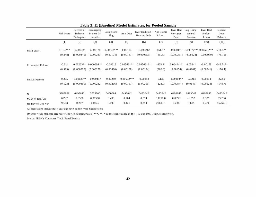
42

Table 3: I1 (Baseline) Model Estimates, for Pooled Sample

Risk ScorePercent of

Balance Delinquent

Bankruptcy in next 24

months

Collections Flag

Any Debt Ever Had Non-Housing Debt

Non-Home Balance

Ever Had Mortgage

Debt

Log Home-secured Balance

Ever Had Student Loans

Student Loan

Balance

(1) (2) (3) (4) (5) (6) (7) (8) (9) (10) (11)

Math years 1.104*** -0.000335 0.000178 -0.00642*** 0.00184 -0.000212 151.9* -0.000176 -0.00877*** 0.00521*** 211.5**

(0.348) (0.000445) (0.000223) (0.00104) (0.00137) (0.000655) (85.20) (0.000231) (0.00228) (0.000970) (78.19)

Economics Reform -0.614 0.00233** 0.000694** -0.00319 0.00568*** 0.00566*** -435.3* 0.00404** 0.0534* -0.00159 -643.7***

(0.593) (0.000992) (0.000278) (0.00496) (0.00188) (0.00134) (206.6) (0.00154) (0.0261) (0.00241) (170.4)

Fin Lit Reform 0.205 -0.00129** -0.000447 0.00240 -0.00632*** -0.00293 6.130 -0.00203** -0.0214 0.00214 222.0

(0.123) (0.000495) (0.000282) (0.00266) (0.00167) (0.00200) (128.0) (0.000844) (0.0146) (0.00124) (148.7)

N 5989930 6493042 5735206 6450004 6493042 6493042 6493042 6493042 6493042 6493042 6493042

Mean of Dep Var 629.2 0.0550 0.00560 0.400 0.764 0.854 11250.8 0.0896 -1.257 0.329 5367.6

Std Dev of Dep Var 93.63 0.207 0.0746 0.490 0.425 0.354 20603.1 0.286 3.685 0.470 16267.3

All regressions include state-year and birth cohort-year fixed effects.

Driscoll-Kraay standard errors are reported in parentheses. ***, **, * denote significance at the 1, 5, and 10% levels, respectively.

Source: FRBNY Consumer Credit Panel/Equifax

43

Table 4: Model I1 Estimates, by Age


Balance Delinquent


months

Collections Flag


Non-Home Balance

Ever Had Mortgage

Debt



Student Loan

Balance

(1) (2) (3) (4) (5) (6) (7) (8) (9) (10) (11)

Mathematics22 year-olds 0.666* -0.0000974 -0.000680 -0.00605*** -0.00200 -0.00364** 39.89 -0.00369*** -0.0437*** 0.00383 123.7**

(0.320) (0.000506) (0.000475) (0.00166) (0.00173) (0.00140) (45.68) (0.000846) (0.00879) (0.00290) (40.65)

25 year-olds 0.165 -0.000333 -0.00110** -0.00949*** 0.00243** 0.00132 384.9** -0.00350*** -0.0322** 0.00658* 397.4**

(0.266) (0.000710) (0.000417) (0.00179) (0.000896) (0.000727) (135.3) (0.000751) (0.0102) (0.00295) (133.4)

27 year-olds -1.365* 0.00253* -0.000549 0.000815 0.00754* 0.00357** 699.0*** -0.00309 -0.0378 0.0157*** 661.9**

(0.565) (0.00109) (0.000704) (0.00349) (0.00326) (0.00122) (147.0) (0.00237) (0.0213) (0.00415) (190.6)

Economics22 year-olds -2.006** -0.000383 -0.000861 0.00133 0.00361 0.00510** 197.1 -0.000860 -0.0260 0.00286 140.2

(0.789) (0.000883) (0.000756) (0.00311) (0.00293) (0.00210) (190.6) (0.00101) (0.0169) (0.00818) (169.7)

25 year-olds -3.094 0.00661** -0.0000632 0.00584 0.00335 0.00385 27.32 0.00101 0.0250 -0.00132 -208.2

(2.388) (0.00281) (0.00149) (0.0114) (0.00329) (0.00337) (179.2) (0.00337) (0.0513) (0.00741) (152.3)

27 year-olds -9.206*** 0.00799** -0.00430* 0.0217*** -0.00520 0.00110 245.9 -0.00561** -0.0653** 0.0126 -7.890

(1.250) (0.00223) (0.00209) (0.00373) (0.00968) (0.00407) (356.1) (0.00202) (0.0249) (0.00954) (311.4)

Financial Literacy22 year-olds -0.926 -0.00365** -0.00247*** 0.0204** -0.0143*** -0.0146*** -11.48 -0.00480*** -0.0505** 0.00575 161.4

(1.126) (0.00122) (0.000398) (0.00829) (0.00195) (0.00112) (177.8) (0.00124) (0.0186) (0.00489) (109.8)

25 year-olds -1.321*** 0.00186*** -0.00205 0.00377 -0.000406 -0.00432* 454.6*** -0.0102*** -0.0912** 0.00740 365.3**

(0.320) (0.000505) (0.00223) (0.00495) (0.00101) (0.00201) (65.56) (0.00269) (0.0275) (0.00797) (112.1)

27 year-olds 0.839 0.00127 0.0000858 -0.00375 0.000596 -0.00350* 627.2*** -0.000625 0.0472 0.000560 435.1**

(0.451) (0.00107) (0.000550) (0.00398) (0.00626) (0.00178) (82.76) (0.00321) (0.0309) (0.00420) (136.8)

Number of Obs22 year-olds 676191 735418 667744 730307 735418 735418 735418 735418 735418 735418 735418

25 year-olds 594217 642849 565420 640338 642849 642849 642849 642849 642849 642849 642849

27 year-olds 471650 508675 431391 506797 508675 508675 508675 508675 508675 508675 508675

Dep. Var. Mean22 year-olds 623.9 0.0519 0.00493 0.381 0.758 0.833 9494.2 0.0337 -1.896 0.306 4523.5

25 year-olds 629.0 0.0583 0.00689 0.482 0.775 0.884 13718.8 0.112 -0.964 0.350 6577.3

27 year-olds 636.9 0.0610 0.00853 0.489 0.778 0.909 15361.6 0.183 -0.179 0.371 7399.4

Dep. Var. Std Dev22 year-olds 91.81 0.201 0.0701 0.486 0.428 0.373 19031.9 0.180 2.331 0.461 11982.6

25 year-olds 96.73 0.211 0.0827 0.500 0.418 0.321 22746.5 0.316 4.122 0.477 18495.4

27 year-olds 99.21 0.217 0.0919 0.500 0.415 0.288 26477.7 0.387 5.045 0.483 22013.3

All regressions include state-year fixed effects.



Online Appendix for

Financial Education and the Debt Behavior of the Young

Meta Brown§, John Grigsby*, Wilbert van der Klaauw‡, Jaya Wen†, and Basit Zafarϯ

The views and opinions offered in this paper do not necessarily reflect the position of the Federal Reserve Bank of New York or the Federal Reserve System. § [email protected]. Research & Statistics. Federal Reserve Bank of New York. *[email protected]. Department of Economics, University of Chicago. ‡ [email protected]. Research & Statistics. Federal Reserve Bank of New York. † [email protected]. Department of Economics, Yale University. ϯ [email protected]. Research & Statistics. Federal Reserve Bank of New York.

mailto:[email protected]





1

A. Curricula Description

This section briefly summarizes the main themes that appear in the curricula of high school financial

literacy and economics courses.

A.1. Financial Literacy Education

Though each state with mandatory high school financial literacy education maintains slightly

different curriculum standards, there are overwhelming similarities in content across state lines, partly due

to a centralized national effort to implement these educational reforms (U.S. Department of the Treasury,

2013; Jumpstart Coalition, 2013). In particular, five central themes appear consistently in state financial

literacy curricula: decision-making, career planning, personal budgeting, borrowing, and investing.1

The first two ask students to consider the relationship between finances and personal financial

goals, and to analyze how career choices impact income, and, as a result, financial constraints. The third

theme, personal budgeting, involves methods of accounting for personal income and expenditures. In this

unit, students employ systems for recording income and spending, learn about different payment methods

like cash or bank cards, and analyze consumer decisions in the context of maintaining a balanced budget

(Indiana Department of Education, 2009; Maryland State Board of Education, 2010; Utah State Office of

Education, 2013; Oklahoma State Department of Education, 2013). Furthermore, students are instructed

on the definition of bankruptcy and ways to improve their credit scores after adverse financial events

(Maryland State Board of Education, 2010; Oklahoma State Department of Education, 2013).

The fourth topic area – borrowing – requires students to “evaluate how to use debt beneficially,

…evaluate the advantages and disadvantages of credit products and services, …analyze sources of

1 See: Personal Financial Responsibility Instruction: Guidelines for Implementation. Indiana Department of Education. http://www.ind-ibea.org/_09_9-2_StBrd_Guidelines_PersFinResp_Approved.pdf ; The Maryland State Curriculum for Personal Financial Literacy Education. Maryland State Board of Education: http://mdk12.org/instruction/curriculum/financial_literacy/financialLiteracy_STANDARDS.pdf ; Personal Financial Literacy. Oklahoma State Department of Education: http://ok.gov/sde/personal-financial-literacy; Instructional Materials Evaluation Criteria – General Financial Literacy. Utah State Office of Education: http://www.schools.utah.gov/CURR/imc/Rubrics-CTE/General-Financial-Literacy.aspx.

http://mdk12.org/instruction/curriculum/financial_literacy/financialLiteracy_STANDARDS.pdf

http://ok.gov/sde/personal-financial-literacy

http://www.schools.utah.gov/CURR/imc/Rubrics-CTE/General-Financial-Literacy.aspx

2

credit,…use numeracy skills to calculate the cost of borrowing, … and analyze credit scores and reports”

(Maryland State Board of Education, 2010; Oklahoma State Department of Education, 2013). Finally, the

last major topic area within state financial literacy introduces students to saving and investment strategies,

relevant quantitative concepts like compound interest and inflation, and frameworks for assessing risk

(Indiana Department of Education, 2009).

A.2. Economic Education

High school economics curricula in nearly all U.S. states require that students understand basic

concepts like scarcity, allocation, maximization subject to a constraint, opportunity cost, marginal benefit,

marginal cost, incentives, trade, comparative advantage, markets, the business cycle, prices, money,

interest rates, income, exchange rates, investment, national accounts, unemployment, and monetary policy

(The State Education Department of New York, 2002; The New Hampshire Department of Education,

2006; The California State Board of Education, 1998; Texas Education Agency, 2010). Frequently, these

concepts are introduced with historical or cultural context: the discussion of national accounts often

incorporates a history of the U.S. federal budget, and a lesson on monetary policy will typically include a

brief history of the Federal Reserve System (The State Department of New York, 2002; Texas Education

Agency, 2010). Likewise, lessons on trade, exchange rates, and comparative advantage are often

complemented by a discussion of international trade and globalization (The New Hampshire Department

of Education, 2006; The State Education Department of New York, 2002). Finally, and perhaps most

relevant in our context, lessons on markets cover topics of supply, demand, prices, and interest rates.

B. Robustness Checks

In this section, we provide additional evidence on the robustness of our findings.

B.1. Impact on the Extensive Margin

To investigate whether financial education impacts the propensity of youth to enter credit markets,

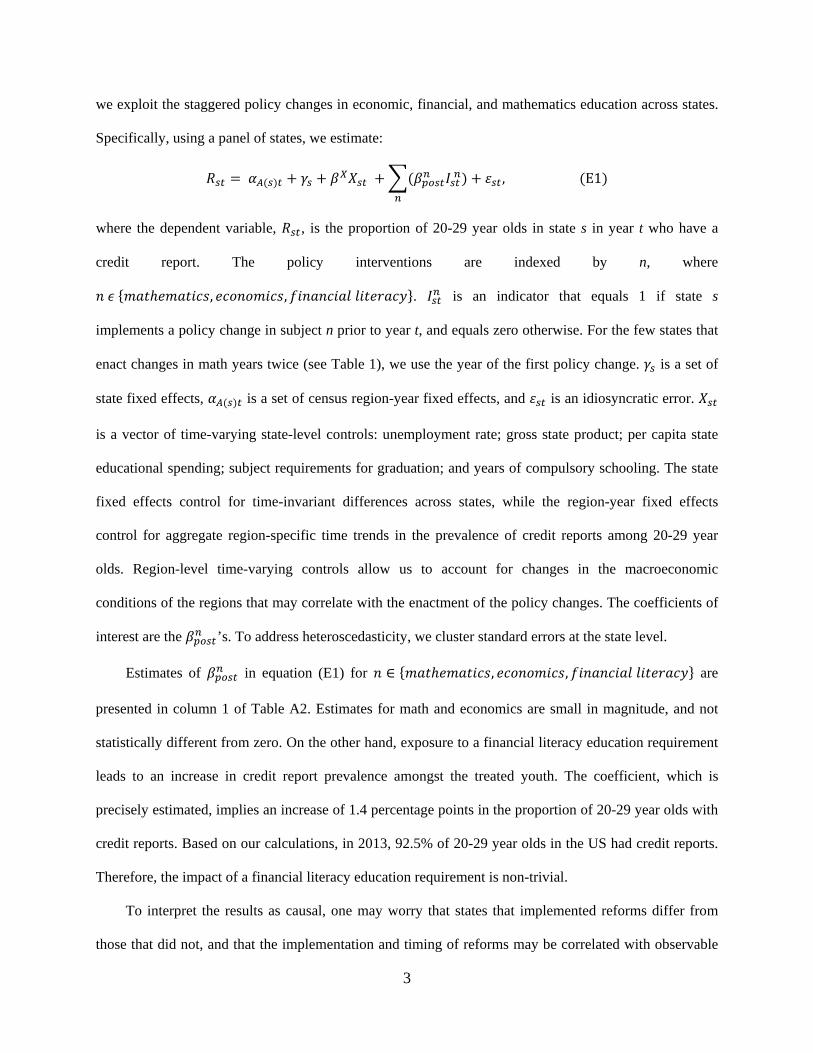
3

we exploit the staggered policy changes in economic, financial, and mathematics education across states.

Specifically, using a panel of states, we estimate:

𝑅𝑅𝑠𝑠𝑠𝑠 = 𝛼𝛼𝐴𝐴(𝑠𝑠)𝑠𝑠 + 𝛾𝛾𝑠𝑠 + 𝛽𝛽𝑋𝑋𝑋𝑋𝑠𝑠𝑠𝑠 + �(𝛽𝛽𝑝𝑝𝑝𝑝𝑠𝑠𝑠𝑠𝑛𝑛 𝐼𝐼𝑠𝑠𝑠𝑠 𝑛𝑛)𝑛𝑛

+ 𝜀𝜀𝑠𝑠𝑠𝑠 , (E1)

where the dependent variable, 𝑅𝑅𝑠𝑠𝑠𝑠, is the proportion of 20-29 year olds in state s in year t who have a

credit report. The policy interventions are indexed by n, where

𝑛𝑛 𝜖𝜖 {𝑚𝑚𝑚𝑚𝑚𝑚ℎ𝑒𝑒𝑚𝑚𝑚𝑚𝑚𝑚𝑒𝑒𝑒𝑒𝑒𝑒, 𝑒𝑒𝑒𝑒𝑒𝑒𝑛𝑛𝑒𝑒𝑚𝑚𝑒𝑒𝑒𝑒𝑒𝑒, 𝑓𝑓𝑒𝑒𝑛𝑛𝑚𝑚𝑛𝑛𝑒𝑒𝑒𝑒𝑚𝑚𝑓𝑓 𝑓𝑓𝑒𝑒𝑚𝑚𝑒𝑒𝑙𝑙𝑚𝑚𝑒𝑒𝑙𝑙}. 𝐼𝐼𝑠𝑠𝑠𝑠𝑛𝑛 is an indicator that equals 1 if state s

implements a policy change in subject n prior to year t, and equals zero otherwise. For the few states that

enact changes in math years twice (see Table 1), we use the year of the first policy change. 𝛾𝛾𝑠𝑠 is a set of

state fixed effects, 𝛼𝛼𝐴𝐴(𝑠𝑠)𝑠𝑠 is a set of census region-year fixed effects, and 𝜀𝜀𝑠𝑠𝑠𝑠 is an idiosyncratic error. 𝑋𝑋𝑠𝑠𝑠𝑠

is a vector of time-varying state-level controls: unemployment rate; gross state product; per capita state

educational spending; subject requirements for graduation; and years of compulsory schooling. The state

fixed effects control for time-invariant differences across states, while the region-year fixed effects

control for aggregate region-specific time trends in the prevalence of credit reports among 20-29 year

olds. Region-level time-varying controls allow us to account for changes in the macroeconomic

conditions of the regions that may correlate with the enactment of the policy changes. The coefficients of

interest are the 𝛽𝛽𝑝𝑝𝑝𝑝𝑠𝑠𝑠𝑠𝑛𝑛 ’s. To address heteroscedasticity, we cluster standard errors at the state level.

Estimates of 𝛽𝛽𝑝𝑝𝑝𝑝𝑠𝑠𝑠𝑠𝑛𝑛 in equation (E1) for 𝑛𝑛 ∈ {𝑚𝑚𝑚𝑚𝑚𝑚ℎ𝑒𝑒𝑚𝑚𝑚𝑚𝑚𝑚𝑒𝑒𝑒𝑒𝑒𝑒, 𝑒𝑒𝑒𝑒𝑒𝑒𝑛𝑛𝑒𝑒𝑚𝑚𝑒𝑒𝑒𝑒𝑒𝑒, 𝑓𝑓𝑒𝑒𝑛𝑛𝑚𝑚𝑛𝑛𝑒𝑒𝑒𝑒𝑚𝑚𝑓𝑓 𝑓𝑓𝑒𝑒𝑚𝑚𝑒𝑒𝑙𝑙𝑚𝑚𝑒𝑒𝑙𝑙} are

presented in column 1 of Table A2. Estimates for math and economics are small in magnitude, and not

statistically different from zero. On the other hand, exposure to a financial literacy education requirement

leads to an increase in credit report prevalence amongst the treated youth. The coefficient, which is

precisely estimated, implies an increase of 1.4 percentage points in the proportion of 20-29 year olds with

credit reports. Based on our calculations, in 2013, 92.5% of 20-29 year olds in the US had credit reports.

Therefore, the impact of a financial literacy education requirement is non-trivial.

To interpret the results as causal, one may worry that states that implemented reforms differ from

those that did not, and that the implementation and timing of reforms may be correlated with observable

4

and unobservable state and cohort factors. To address these concerns, E1 allows for census region-

specific time trends, state fixed effects, and a rich set of time-varying state-level controls. E1, however,

assumes that credit prevalence in states that implement a reform (treatment group) and those that do not

(control) would trend similarly in the absence of the reforms. While this counterfactual is not inherently

testable, the panel data allow us to test whether states that implement policy changes were trending

similarly in the years prior to the adoption of the reform to those that did not implement a policy change.

Therefore, as an additional check, we estimate the following specification which allows for the possibility

of a different average pre-reform trend in states that enacted a policy change, relative to those that did not:

𝑅𝑅𝑠𝑠𝑠𝑠 = 𝛼𝛼𝐴𝐴(𝑠𝑠)𝑠𝑠 + 𝛾𝛾𝑠𝑠 + 𝛽𝛽𝑋𝑋𝑋𝑋𝑠𝑠𝑠𝑠 + �(𝛽𝛽𝑝𝑝𝑝𝑝𝑝𝑝𝑛𝑛 𝑃𝑃𝑠𝑠𝑠𝑠 𝑛𝑛 + 𝛽𝛽𝑝𝑝𝑝𝑝𝑠𝑠𝑠𝑠𝑛𝑛 𝐼𝐼𝑠𝑠𝑠𝑠 𝑛𝑛)𝑛𝑛

+ 𝜀𝜀𝑠𝑠𝑠𝑠 . (E2)

This specification has an additional term compared to E1: 𝑃𝑃𝑠𝑠𝑠𝑠𝑛𝑛 , which equals 1 if state s implements a

policy change in subject n in or after year t, and is zero otherwise. This variable allows us to test whether

treated and control states had similar average pre-trends. A suggestive test of the common trend

assumption is that the pre-treatment coefficient 𝛽𝛽𝑝𝑝𝑝𝑝𝑝𝑝𝑛𝑛 is zero. When presenting the results, we instead

show estimates of (𝛽𝛽𝑝𝑝𝑝𝑝𝑠𝑠𝑠𝑠𝑛𝑛 − 𝛽𝛽𝑝𝑝𝑝𝑝𝑝𝑝𝑛𝑛 ); an estimate statistically different from zero would show a break of the

trend in credit prevalence amongst youth after the enactment of the policy, and would be evidence of a

causal effect of the policy.

The second column of Table A2 reports estimates of (𝛽𝛽𝑝𝑝𝑝𝑝𝑠𝑠𝑠𝑠𝑛𝑛 − 𝛽𝛽𝑝𝑝𝑝𝑝𝑝𝑝𝑛𝑛 ). We see that the estimates are

very similar to the E1 estimates. This suggests that the common trends assumption may not be

problematic in this context. Overall, these findings indicate that the math and economic education

requirements have no impact on the extensive margin, while financial literacy education requirements

lead to a small (and precisely estimated) increase in the prevalence of credit reports. Since the impact of

requiring financial education on the extensive margin is quite small, it is unlikely that the impacts that we

find on the intensive margin (that is, the credit report outcomes) are a result of the compositional changes

in credit report holders.

5

B.2. Multiple Testing Corrections

Our empirical analysis employs eleven dependent variables, and hence testing for the impact of a

reform on outcomes involves the simultaneous testing of several hypotheses. In the analysis so far, we

have not taken the multiplicity of tests into account. This can be problematic because the probability that

some false hypothesis is accepted by chance alone can be quite large in such cases. For example, tests of

the relationship between financial education and bankruptcy and number of accounts in

collection are clearly not independent. The case of eleven independent tests provides an upper

bound on the odds of accepting a false hypothesis. 2

Being mindful of the potential for false positives, we next employ a multiple testing correction to

our p-values and adjust them downward, in an effort to minimize false findings. The correction that we

apply is the Benjamini-Hochberg False Discovery Rate, which is fairly standard in the literature of

multiple hypotheses testing (see, for example, Romano, Shaikh, and Wolf, 2010). It is implemented

by ranking all the coefficients by p-value from smallest p-value to largest. The largest p-value remains

unchanged. The second-largest p-value is multiplied by the number of ex-ante null hypotheses (N=11)

divided by its rank (N-1, that is, 10), and so on.3

The first column of Table A3 reports the p-value of each significant coefficient in our baseline I1

model for the pooled sample (Table 3). Column (2) shows the corrected p-values. We see that nearly all

of our estimates from the baseline specification that were found to be statistically different from zero at

the ten percent level or below, continue to be so at the 12% level or higher; the only exception being non-

housing debt balance for math years, with an adjusted p-values of at 0.18. Hence we conclude that our

conclusions are robust to correcting for multiple hypothesis testing.

2 For example, if 10 hypotheses are being tested at the same time, one expects one true null hypothesis to be falsely rejected at the 10% level. Further, if all tests are mutually independent, then the probability that at least one true null hypothesis will be rejected at the 10% level is 1 − 0.910 = 0.65. 3 There are other correction methods, such as the Bonferroni correction. It makes the very conservative assumption that the null hypotheses are uncorrelated. Since many aspects of consumer credit behavior are intimately linked, we believe the Bonferroni correction is not appropriate for our setting.

6

B.3. Falsification Test

As a further investigation of whether our results reflect the true impact of educational reforms,

we perform the following falsification exercise. We draw a sample of respondents born between 1971

and1980 from the Consumer Credit Panel (note the sample used in the main analysis are individuals born

in or after 1981). These individuals would have turned 18 before 1999. Under our definition, they would

have graduated from high school prior to 1999, and hence would not have been impacted directly by the

economics and financial literacy reforms that we focus on. We then randomly assign them to states. The

reason for not using the respondent’s actual state is to allow for the possibility that there may be spillover

effects (say, from younger siblings who are actually exposed to our reforms). The reform dates are then

shifted earlier by ten years. This simulates the counterfactual where cohorts born ten years earlier were

exposed to reforms in those states (to which individuals are randomly assigned).

We estimate model I1 on this placebo reform sample; estimates are presented in Table A4. If the

pattern of consumer credit behavior elucidated in our results is truly the result of the education reforms,

repeating our baseline analysis on the panel with fictitious timing should yield coefficients that are either

zero, or significantly different from our baseline estimates. Looking at the estimates for economics

education, all the estimates that are significant have a sign opposite to that of the actual baseline estimates

in Table 3 (except for student loan balance, which is only marginally significant). Further, the significant

coefficient estimates are generally an order of magnitude or more smaller than the significant baseline

estimates, in terms of their absolute magnitude. In the case of financial literacy, all estimates except

bankruptcy are not statistically different from zero. And even for bankruptcy, the estimate is of the sign

opposite to that in the baseline and of comparatively small magnitude. Thus, this falsification gives us a

greater degree of confidence that our baseline results capture the true effect of educational reforms rather

than other confounding effects.

7

B.4. The CARD Act

One potential concern is that our estimates may be biased by the Credit Card Accountability and

Responsibility and Disclosure (CARD) Act of 2009, which affected provision of credit to individuals

younger than 21 (see Agarwal, Chomsisengphet , Mahoney, and Stroebel (2013), and Debbaut, Ghent,

and Kudlyak (2013) for discussion and evaluation of the Act). Stango and Zinman (2011), for

example, demonstrate a substantial effect of the Truth-in-Lending Act on consumer interest rates.

Hence one might be concerned that the CARD Act impacted young borrowers’ debt profiles

meaningfully.

Since our identification exploits time by cohort by state variation, and the Act affects only the

youngest cohorts after 2009 in a manner that varies by state, this could be an issue. While the Act was

implemented in phases, the provisions of the Act that affected credit access to youth under the age of 21

took effect in early 2010. Therefore, as a sensitivity check, we re-estimate our baseline model using data

through 2009 only. As a result, younger cohorts are dropped from the analysis. Estimates are presented in

Table A5. The estimates for Math are qualitatively similar, with the exception of the non-home and

housing debt balance variables which switch signs. In the case of economics education, estimates are

similar and in most cases larger in magnitude and more precise than the baseline estimates. For example,

the impact on risk scores is now a significant decline of 3 points (compared to an imprecise decline of 0.6

points in the baseline model). The only estimate that is meaningfully different between the two is the

prevalence of student loans which becomes positive now. This may arguably be a result of us dropping

the period of the sample where student loans take off in the population. The finding that restricting the

analysis to older cohorts generally strengthens the impacts of economics education should not be

surprising, since Table 4 shows that age-specific estimates for economics strengthen over time. Results

regarding financial education are qualitatively similar to those using the full sample period. Overall, this

check suggests that the CARD Act requirements are not biasing our estimates.

8

B.5. Combined Effect of Economics and Financial Education Reforms

The estimated models implicitly assume that the effect of financial literacy and economics

education is additive. Since some cohorts in certain states are exposed to both subjects, while others are

exposed to only one of them, we can directly test whether that is the case. Table 2, for example, shows

that 42.5% of the sample individuals were only exposed to economic education, with 11.1% also being

exposed to financial literacy education concurrently. We estimate a variant of equation (I1), where now 𝑛𝑛

in the term ∑ (𝛽𝛽𝑝𝑝𝑝𝑝𝑠𝑠𝑠𝑠𝑛𝑛 𝐷𝐷𝑖𝑖(𝑠𝑠𝑠𝑠)𝑛𝑛

𝑛𝑛 ) denotes {economics only, financial literacy only, both economic and financial

literacy}. 𝐷𝐷 𝑖𝑖(𝑠𝑠𝑠𝑠) 𝑝𝑝𝑠𝑠𝑝𝑝𝑛𝑛 𝑝𝑝𝑛𝑛𝑜𝑜𝑜𝑜, for example, equals 1 if i of birth cohort c was exposed to economic education (but

not financial literacy) when in high school in state s, and zero otherwise.

Estimates are reported in Table A6. The first three rows can be compared to those in the baseline

model (shown in Table 3). Estimates for exposure to only economics reform are quantitatively similar to

those for economics in Table 3. Likewise for exposure to financial literacy only, estimates – except for

proportion of balance that is delinquent and non-home balance – are quite similar to those in the baseline

model; it may be worth noting that financial literacy education absent economics education is estimated to

increase mean risk scores by almost a full point, and this is significant at the ten percent level. The

coefficients of interest here are in the fourth row of the table, which reports the estimates of joint

exposure to economics and financial literacy education. If the additive assumption in our earlier

specifications is correct, these estimates should be roughly similar to the sum of the coefficients for

economics and financial literacy education in Table 3. That is in fact what we find. Moreover, since

economics and financial literacy often have opposite effects with economics’ impacts being larger in

magnitude (see Table 3), the estimates for exposure to the joint reforms are often similar in sign to those

for economics. Overall, the patterns in the table suggest that the impacts of the two types of education –

economics and financial literacy – do not interact, and that our additive assumption is quite reasonable in

this context.

9

References Agarwal, Sumit, Souphala Chomsisengphet, Neale Mahoney, and Johannes Stroebel. 2013. Regulating Consumer Financial Products: Evidence from Credit Cards. Working Paper, New York University. Debbaut, Peter, Andra Ghent, and Marianna Kudlyak. 2013. Are Young Borrowers Bad Borrowers? Evidence from the Credit CARD Act of 2009. Working Paper. Romano, Joseph, Azeem Shaikh, and Michael Wolf (2010). Hypothesis Testing in Econometrics. Annual Review of Economics, Vol. 2, p. 75-104.

10

Table A1: Mobility of young credit report holders

Age% of individuals living in the same state as at age

18

19 98.87%20 97.33%21 95.75%22 93.72%23 91.27%24 89.00%25 87.18%26 85.55%27 84.18%28 83.01%29 82.06%

Source: FRBNY Consumer Credit Panel

11

Table A2: Impact of Financial Education on the Extensive Margin

Baseline Event Study(1) (2)

Financial 0.0142*** 0.0151**Literacy Reform (0.00506) (0.0058)

Economics -0.00231 0.00212Reform (0.00681) (0.0062)

Math years -0.000111 -0.000123Reform (0.00596) (0.006)

Observations 594 594Mean of Dep Var 0.595 0.595Std of Dep Var 0.304 0.304

Dependent variable is the proportion of 20-29 year olds in a state-year. All regressions include region * year fixed effects, and standard errors clustered at the state level. Standard errors reported in parentheses. ***, **, * denote significance at the1, 5, and 10% level, respectively. Coefficients in Column 2 reflect difference between pre- and post-reform dummies. Source: FRBNY Consumer Credit Panel/Equifax

12

Table A3: Adjusted p-values for the Baseline Model Estimates

Rank Variable Standard Benjamini-Hochberg(1) (2)

Mathematics Years

1 Collections Flag 0.000 0.002 Ever Had Student Loans 0.000 0.003 Log Home-Secured Balance 0.002 0.014 Risk Score 0.007 0.025 Student Loan Balance 0.017 0.046 Non-Home Balance 0.096 0.18

Financial Literacy Reform

1 Any Debt 0.002 0.022 Percent of Balance 0.021 0.123 Ever Had Mortgage Debt 0.030 0.11

Economics Reform

1 Ever Had Non-Home Debt 0.001 0.012 Student Loan Balance 0.002 0.013 Any Debt 0.009 0.034 Ever Had Mortgage Debt 0.020 0.065 Bankruptcy in Next 24 0.027 0.066 Percent of Balance 0.034 0.067 Non-Home Balance 0.054 0.088 Log Home-Secured Balance 0.060 0.08

Table reports corrected p-values for estimates of the I1 model that are statistically significant at the 10% or higher level in the baseline (Table 3)

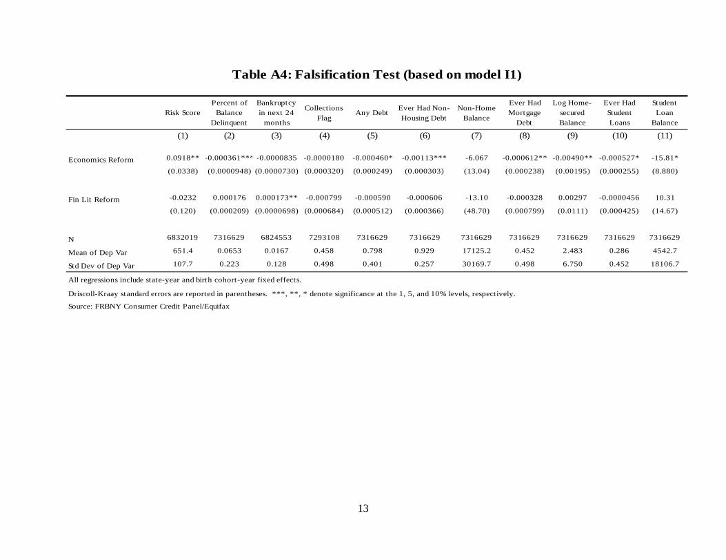
13

Table A4: Falsification Test (based on model I1)


Balance Delinquent


months

Collections Flag


Non-Home Balance

Ever Had Mortgage

Debt



Student Loan

Balance

(1) (2) (3) (4) (5) (6) (7) (8) (9) (10) (11)

Economics Reform 0.0918** -0.000361*** -0.0000835 -0.0000180 -0.000460* -0.00113*** -6.067 -0.000612** -0.00490** -0.000527* -15.81*

(0.0338) (0.0000948) (0.0000730) (0.000320) (0.000249) (0.000303) (13.04) (0.000238) (0.00195) (0.000255) (8.880)

Fin Lit Reform -0.0232 0.000176 0.000173** -0.000799 -0.000590 -0.000606 -13.10 -0.000328 0.00297 -0.0000456 10.31

(0.120) (0.000209) (0.0000698) (0.000684) (0.000512) (0.000366) (48.70) (0.000799) (0.0111) (0.000425) (14.67)

N 6832019 7316629 6824553 7293108 7316629 7316629 7316629 7316629 7316629 7316629 7316629

Mean of Dep Var 651.4 0.0653 0.0167 0.458 0.798 0.929 17125.2 0.452 2.483 0.286 4542.7

Std Dev of Dep Var 107.7 0.223 0.128 0.498 0.401 0.257 30169.7 0.498 6.750 0.452 18106.7




14

Table A5: Baseline Model Estimated till 2009 (CARD Act Robustness)


Balance Delinquent


months

Collections Flag


Non-Home Balance

Ever Had Mortgage

Debt



Student Loan

Balance

(1) (2) (3) (4) (5) (6) (7) (8) (9) (10) (11)

Math years 0.971 -0.00112 -0.0000863 -0.00386*** 0.000206 0.00119 -78.56*** 0.000342 0.0000613 0.00336* 11.02

(0.585) (0.000681) (0.000267) (0.000874) (0.00167) (0.00100) (14.24) (0.000452) (0.00686) (0.00150) (26.58)

Economics Reform -3.012*** 0.00409** 0.00215*** 0.00387 0.0111* 0.00919** -58.35 0.00455 0.0762* 0.0184** -545.7

(0.695) (0.00138) (0.000494) (0.00686) (0.00546) (0.00403) (427.0) (0.00335) (0.0415) (0.00792) (323.6)

Fin Lit Reform 0.182 -0.00184 0.0000203 -0.00167 -0.0106*** -0.00786** 163.1 -0.00329*** -0.0289*** 0.000416 514.3***

(0.514) (0.00116) (0.000186) (0.00499) (0.00302) (0.00252) (174.6) (0.000428) (0.00771) (0.000738) (140.0)

N 2814496 3062497 3042069 3043006 3062497 3062497 3062497 3062497 3062497 3062497 3062497

Mean of Dep Var 621.9 0.0587 0.00680 0.381 0.764 0.838 10047.6 0.0752 -1.417 0.271 3919.0

Std Dev of Dep Var 94.24 0.212 0.0822 0.486 0.425 0.368 18719.7 0.264 3.412 0.444 12906.3




15

Table A6: Baseline Model, with Combined Effects for Economics and Financial Literacy Education


Balance Delinquent


months

Collections Flag


Non-Home Balance

Ever Had Mortgage

Debt



Student Loan

Balance

(1) (2) (3) (4) (5) (6) (7) (8) (9) (10) (11)

Math years 1.106*** -0.000331 0.000178 -0.00643*** 0.00183 -0.000213 151.0* -0.000185 -0.00883*** 0.00522*** 210.9**

(0.349) (0.000446) (0.000223) (0.00105) (0.00138) (0.000653) (84.66) (0.000239) (0.00230) (0.000968) (77.95)

Economics Reform Only -0.495 0.00263*** 0.000579** -0.00361 0.00446* 0.00558*** -515.9** 0.00330 0.0478 -0.000745 -693.1***

(0.648) (0.000879) (0.000251) (0.00523) (0.00231) (0.00147) (210.2) (0.00189) (0.0305) (0.00263) (171.9)

Fin Lit Reform Only 0.923* 0.000490 -0.00119 -0.000159 -0.0136*** -0.00344 -476.2*** -0.00642*** -0.0550*** 0.00719* -73.87

(0.432) (0.00105) (0.000796) (0.00145) (0.00318) (0.00411) (154.2) (0.00116) (0.0107) (0.00381) (126.8)

Econ & Fin Lit Reform -0.514 0.000791 0.000357 -0.000416 0.000415 0.00280 -359.6** 0.00263*** 0.0368*** -0.000174 -379.0***

(0.509) (0.000757) (0.000529) (0.00379) (0.00163) (0.00191) (150.4) (0.000705) (0.00902) (0.00280) (123.7)

N 5989930 6493042 5735206 6450004 6493042 6493042 6493042 6493042 6493042 6493042 6493042

Mean of Dep Var 629.2 0.0550 0.00560 0.400 0.764 0.854 11250.8 0.0896 -1.257 0.329 5367.6

Std Dev of Dep Var 93.63 0.207 0.0746 0.490 0.425 0.354 20603.1 0.286 3.685 0.470 16267.3


