Embed Size (px)
Citation preview

Finding Common RNA Pseudoknot Structures in Polynomial Time
Patricia Evans
University of New Brunswick

6-Jul-2006 2
Ribonucleic Acid (RNA) RNA is an organic molecule that forms long
chains Each position in the chain can be one of 4 types
(bases): A, G, C, U RNA can code gene information (messenger
RNA, viral RNA) RNA can also form structures and take many
functions within a cell (eg. tRNA, rRNA and other RNA-protein complexes)

6-Jul-2006 3
RNA Bonds and Structures RNA bases can form bonds, in a largely
pairwise fashion (A-U, G-C, some exceptions) RNA is single stranded; its bonds form mostly
within a single chain, folding it into a complex structure held together by its bonds
RNA function is affected by its structure If two bases are paired, it often does not matter what
they are; only unpaired bases are ‘available’ Common substructures can help investigate
functional relationships

6-Jul-2006 4
RNA Structural Complexity Deceptively simple, since bases are usually paired Stems are formed from two bonded strands, in an
antiparallel orientation These simple bonds can however combine to form
complex structures Some are nested (stems within loops) Some are knotted (stems effectively crossing)
RNA molecules can be very long (eg. > 1000 bases), confounding exhaustive comparison techniques

6-Jul-2006 5
Arc Representation At a bond level, the bond structure of an RNA
molecule can be represented as arcs superimposed onto the “stretched” RNA sequence.
Each arc represents a bonded pair, and the structure is a set of pairs.
Nested Structure Pseudoknot

6-Jul-2006 6
Maximum Common Ordered Substructure
Input: Structures S1 and S2, where each structure is a set of pairs over n1 and n2 positions (resp.)
Output: max. substructure Sc with nc positions, such that there exist 1-1 functions f1 and f2 where:f n n f n nc c1 1 2 21 1 1 1:{ , . . . , } { , . . . , } , :{ , . . . , } { , . . . , }
i j n i j f i f j f i f jc, { , . . . , } : ( ) ( ) ( ) ( )1 1 1 2 2
( , ) ( ), ( ) ( ), ( )i j S f i f j S f i f j Sc 1 1 1 2 2 2

6-Jul-2006 7
General Structures are Hard The general MCOS problem, allowing positions to bond
multiple times, is NP-hard (Goldman et al., 1999) Comparing two RNA (pair-bond) structures is
polynomial if they do not have knots (Bafna et al., 1995) A structure S has a knot if and only if:
there are pairs (i1, j1) and (i2, j2) in S where
i1 < i2 < j1 < j2
( [ ) ]
Comparing knotted arc structures is NP-hard for arbitrary pair-bond structures (Evans 1999, and others)

6-Jul-2006 8
Comparing Knot-Free StructuresIf the two structures are composed only of nested bonds, they
can be compared in O(n4) time using a dynamic programming algorithm that computes:
M[i1, j1, i2, j2] = max { M[i1, j1-1, i2, j2] , M[i1, j1, i2, j2-1] ,
M[i1, k1-1, i2, k2-1] + M[k1+1, j1-1, k2+1, j2-1] +1
if (k1, j1) is in S1
and (k2, j2) is in S2 }our answer is in M[0,|A|-1,0,|B|-1](result: Bafna et al. 1995)

6-Jul-2006 9
Limited Context
The polynomial time DP algorithm for nested bond structures works due to the context-free nature of segments in the nested structures.
Knotted structures have segments that are not context-free, but we can limit the context that they need if we consider special cases that cover most known RNA structures.

6-Jul-2006 10
Pseudoknot Observations Three mutually crossing arcs generally do not
occur in RNA structures (3-knot)
A structure without 3-knots can be separated into 2 layers of non-crossing arcs (2-colourable)

6-Jul-2006 11
Pseudoknot Observations
Crossing arcs tend to be grouped into crossing stems, though there can be some nesting
Interleaving between left and right endpoints does not usually occur, and would be biochemically unstable

6-Jul-2006 12
Forming LSPsTo take advantage of these restrictions, we will
consider that bonds group into stems, and that a stem can break the RNA sequence into linked segment pairs (LSPs): a matched pair of segments that are, or may be, linked by bonds.
i j h l i j
Segment LSP: an ordered segment pair

6-Jul-2006 13
Merging LSPs
The key to the use of LSPs is our ability to merge them to construct a larger LSP, as shown.
The restrictions allow us to consider only pairwise LSP merges – we can always fill at least one existing “hole” when we merge.

6-Jul-2006 14
Structure Pieces
We can then consider two types of comparison cases, and build up our results from them:
Segment-to-segment (4 dimensions) LSP-to-LSP (8 dimensions)We do not need to match LSPs to segments,
as long as we allow both segments and LSPs to be broken into parts.

6-Jul-2006 15
Segment CasesSegment cases are based on the BMR95 algorithm.
s1: value of matching segment (i1, j1-1) to (i2, j2) s2: value of matching segment (i1, j1) to (i2, j2-1) s3: if j1 links to k1 and j2 links to k2: 1 + (value of matching segment (i1, k1-1) to (i2, k2-1)) + (value of matching segment (k1+1, j1-1) to (k2+1, j2-1))
6-Jul-2006 16
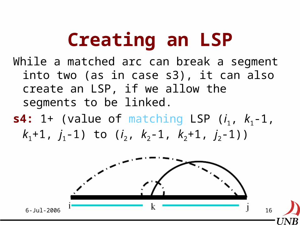
Creating an LSPWhile a matched arc can break a segment into two
(as in case s3), it can also create an LSP, if we allow the segments to be linked.
s4: 1+ (value of matching LSP (i1, k1-1, k1+1, j1-1) to (i2, k2-1, k2+1, j2-1))

6-Jul-2006 17
LSP Cases – Simple
The first cases for matching LSPs are based on the segment matching: two paring and one split.
a1: value of matching LSP (h1,l1,i1, j1-1) to (h2,l2,i2, j2) a2: value of matching LSP (h1,l1,i1, j1) to (h2,l2,i2, j2-1) a3: (value of matching segment (h1, l1) to (h2, l2)) + (value of matching segment (i1, j1) to (i2, j2))
Case a3 can be used with s4 to allow new LSPs to be made from right segments of matched LSPs.

6-Jul-2006 18
LSP Cases – Within RightIf the arcs link to positions within the right side of the LSPs, then the segments within the arcs can be the right sides of new LSPs.
a4: 1 + (value of matching LSP (h1,l1,k1+1, j1-1) to (h2,l2, k2+1, j2-1)) + (value of matching segment (i1, k1-1) to (i2, k2-1))

6-Jul-2006 19
LSP Cases – Within Right
Alternatively, the arcs could bound segments that are within the structure of the right side of the LSPs.
a5: 1 + (value of matching LSP (h1, l1, i1, k1-1) to (h2, l2, i2, k2-1)) + (value of matching segment (k1+1, j1-1) to (k2+1, j2-1))

6-Jul-2006 20
LSP Cases – Cross LeftIf the arcs cross to the left side of the LSPs, then their left endpoints (k) can form a hole to start new LSPs.
a6: 1 + (value of matching LSP (h1,k1-1, k1+1, l1) to (h2,k2-1, k2+1, l2)) + (value of matching segment (i1, j1-1) to (i2, j2-1))

6-Jul-2006 21
LSP Cases – Cross LeftThe arcs can instead separate the LSP within them from initial segments.
a7: 1 + (value of matching LSP (k1+1,l1,i1, j1-1) to (k2+1,l2,i2, j2-1)) + (value of matching segment (h1, k1-1) to (h2, k2-1))
We do not try to link the first and third segments as they would form part of a 3-knot.

6-Jul-2006 22
LSP Cases – Cross Left
Matched arcs can break the LSPs into three segments.
a8: 1 + (value of matching segment (h1, k1-1) to (h2, k2-1)) + (value of matching segment (k1+1, l1) to (k2+1, l2))
+ (value of matching segment (i1, j1-1) to (i2, j2-1))

6-Jul-2006 23
LSP Cases – Crossed LSPsArcs crossing existing LSPs could need a merging of the LSP types in a6 and a7 – but then we need to consider all places for the split to occur.
a9: 1 + max [over all s1,s2 with k1<s1<l1, k2<s2<l2] (value of matching LSP (h1,k1-1, s1+1,l1) to (h2,k2-1, s2+1,l2)) +(value of matching LSP (k1+1,s1,i1, j1-1) to (k2+1,s2,i2, j2-1))

6-Jul-2006 24
Dynamic Programming
These cases take care of all possibilities for how LSPs and segments can be broken down, and their results merged.
They can be turned straightforwardly into a dynamic programming algorithm that uses two tables (one for segments, one for LSPs)
The algorithm will need to weave between these two tables in a way consistent with the data

6-Jul-2006 25
Making It Feasible
This algorithm makes very heavy use of multidimensional dynamic programming tables, and looks more of theoretical interest than practical use. Time complexity is high at O(n10) Space complexity is even more crucial at O(n8)
Careful implementation is needed to avoid these theoretical worst cases.

6-Jul-2006 26
Engineering Space and Time Space and time usage can be minimised by eliminating
those computations that are not needed. The recurrence should be computed recursively (using
memoisation) to enable the data to help this pruning Note that most segment pairs will not correspond to LSPs
consistent with a given arc structure The table can be allocated dynamically, in layers, so
that a hyperplane of the table is only allocated if it will contain an entry (and note h < l < i < j )
We can reduce this further by limiting hyperplane sizes to the corresponding segment within an arc

6-Jul-2006 27
Experiments Having reduced the space, experiments were run on a
variety of RNA structural data to determine if the algorithm is of practical use Large Subunit ribosomal RNA structures RNAse P structures Mosaic Virus structures
Structures of up to 400 arcs were compared effectively in 4Gb of space, with correct substructures found allocating about 10-14 of the theoretical table Even the O(n4) recurrence for unknotted structures would
need too much space without the space saving technique

6-Jul-2006 28
Conclusion and Future Work Under these restrictions, RNA bond structures can be
compared in polynomial time With careful case pruning, the algorithm is feasible
and produces useful results The problem of comparing general 2-colourable bond
structures (allowing endpoint interleaving) is still open Extensions to pattern discovery for multiple structures
can be explored Weights can be added to model RNA more accurately


![Notes on Polynomial Functors - UAB Barcelonakock/cat/polynomial.pdf · 2018. 1. 11. · • Polynomial functors and polynomial monads [39] with Gambino • Polynomial functors and](https://img.pdfslide.net/doc/110x75/60faf8a63b5d714a860ca184/notes-on-polynomial-functors-uab-barcelona-kockcat-2018-1-11-a-polynomial.jpg)