Embed Size (px)
Citation preview
Finding Moving Evaders in Terrains Using a Chain of Seekers
Parrish Myers University of Arizona
Gould-Simpson Building Room 742 Tucson, AZ 85721 1 (520) 250-3849
Swaminathan Sankararaman University of Arizona
Gould-Simpson Building Room 749 Tucson, AZ 85721 1 (520) 621-2738
Alon Efrat University of Arizona
Gould-Simpson Building Room 742 Tucson, AZ 85721 1 (520) 626-8047
ABSTRACT In this paper, we propose algorithms for computing optimal trajectories of a group of flying observers (such as helicopters or UAVs) searching for a lost child in a hilly terrain. Very few assumptions are made about the speed or direction of the child’s motion and whether it might (either deliberately or accidentally) try to avoid begin found. This framework can also be applied to a set of seekers searching for hostile evaders such as smugglers/criminals, or friendly evaders such as lost hikers. We show how to plan trajectories (locations and velocities) of each of the seekers so as to maximize the probability that the child is found, while coordinating the motion of the seekers to include constraints based on: visibility region of the seekers, determined by line of sight limitations due to terrain features; and operational time of seekers. Our algorithm explores useful I/O-efficient data structures and branch-cutting techniques to achieve further speedup in execution time by limiting the storage requirements and total number of graph nodes searched, respectively.
Categories and Subject Descriptors I.2.9 [Artificial Intelligence]: Robotics - Autonomous vehicles, sensors, workcell organization and planning.
General Terms Algorithms, Performance, Experimentation.
Keywords Algorithms, UAV, coordinated route planning, branch-cutting, sensors, I/O-efficient data structures.
1. INTRODUCTION In this paper we propose solutions for a set of optimization problems, demonstrated by the following example. A young child is lost in hilly terrain. Her actions are unpredictable and location unknown, but constrained to a known region of terrain. A team of rescuers needs to be assembled, to conduct a search for her. With the recent decrease in the cost of unmanned areal vehicles (UAV), and the increase in their capabilities, suggests the possibility that multiple (possibly a large number of) areal vehicles could participate. Due to the child’s mobility, and possibly its intentional avoidance to being found, a careful synchronization between the UAVs’ movements is needed to guarantee that she will be found as soon as possible. In this paper we present an algorithm for finding the UAVs’ trajectories, and their synchronized motion along their trajectories, in a way that maximizes the probability that the child would be found in the shortest period while minimizing resources such as fuel consumptions so as to increase their operational time.
This framework can also be applied to a set of seekers searching for lost hikers, after smugglers or terrorist, or similar military settings. For generality, we would use the terms evader, and seekers, rather than child and UAVs. We next look at the constraints governing the search. To find the evader, one of the seekers, must be able to detect it. This limits the elevation above the surface and distances between the seekers. In particular, mountains or other terrain features must not occlude the child from all seekers. However, even having a line of sight to the evader might not be a sufficient condition for finding it. Vegetation (trees, bushes), and limitations of the optical or thermal imaging devices used by the seekers also limits the visibility. To consider extreme cases using helicopters: maximum elevation might allow the entire search area to be seen from a single point, but angular resolution of the imaging device and poor visibility might prevent the seeker from distinguishing enough details to detect the evader. On the other extreme, flying helicopters at ground level is also problematic, since the region they could search is much smaller, and requires more maneuvers than would be unnecessary at higher elevations. We would assume that there is an optimal elevation λ above the terrain surface, which is optimal for the search, and would design seekers’ trajectories according to terrain features, trying to keep them at this elevation.
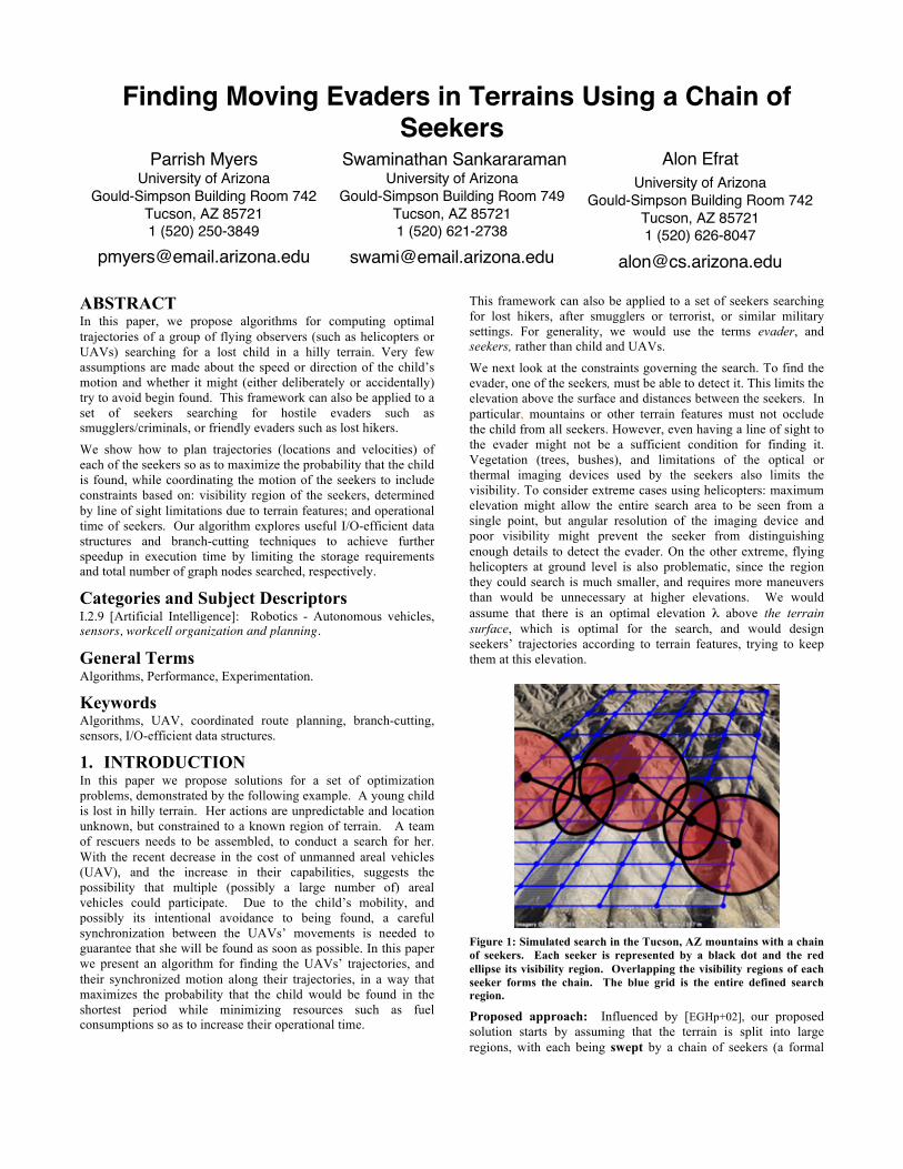
Figure 1: Simulated search in the Tucson, AZ mountains with a chain of seekers. Each seeker is represented by a black dot and the red ellipse its visibility region. Overlapping the visibility regions of each seeker forms the chain. The blue grid is the entire defined search region.
Proposed approach: Influenced by [EGHp+02], our proposed solution starts by assuming that the terrain is split into large regions, with each being swept by a chain of seekers (a formal

definition is below). The term “sweep” here means that the seekers always form a chain and separate the terrain (or a portion of the terrain) into two distinct areas, commonly called the clean region, already searched and no possibility of evader occupying this area; and contaminated region, yet to be searched and possibly containing the evader. See Figure 1 for an illustration.
At the beginning of the process, the contaminated region occupies the whole terrain. As the chain moves (sweeps) the terrain, the clean region deforms continuously (not necessarily monotonically) until it occupies the whole terrain. The seekers are always positioned so that their visibility regions (the portion of the terrain each one monitors at each moment) overlap, so the child could not “sneak” between two of them without being noticed. It is clear that as long as the child is in the terrain and is (at least partially) visible, this search strategy is guaranteed to find it, independent of its pattern of motion. The question then becomes: given a hilly terrain, what is the best motion of the chain of rescuers to minimize expenditure of resources, but still thoroughly search the region.
Natural criteria for optimization that come to mind include (i) minimizing the horizontal distance between the seeker and each point it surveys, (ii) minimizing horizontal distance between each seeker and the following seeker, (iii) minimizing fuel needed, (iv) minimizing time. Minimizing fuel depends on a variety of parameters, but factors that are relevant are, total time, velocity and elevation gain. Minimizing the time is related not only to the constraints of the seeker itself, but also to time that the each seeker needs to spend to obtain the synchronized motion of all seekers forming the chain. Sweeping the terrain could be accomplished using many geometric patterns, possibly optimizing different cost functions.
Figure 2: Options for searching through a series of mountains while maintaining elevation λ above the terrain: (a) optimal configurations show at times t1 and t2 to minimize elevations changes; (b) poor choice if elevation changes should be kept to a minimum.
Figure 2 demonstrates two different sweeping patterns of the same synthetic terrain. This terrain consists of 3 mountain ridges, which are assumed to be at a maximum elevation E, and the valleys in between are at elevation 0. Two natural ways to perform the sweep are by flying from south to north (Figure 2a) or from east to west (Figure 2b). In both cases, each seeker is always at elevation α above the terrain, where λ is a constant as above. Both strategies would sweep the terrain. However, if the major component of the cost is the elevation gain, then the first method is probably preferable, since each helicopter changes its height at most once and gains a total height that for some seekers is λ, and for the others it is E+λ as they only need to reach the ridge of the mountain, on which it could fly horizontally. In the second approach (Figure 2b) each one of the seekers need to gain an elevation of 3E+λ, since it needs to “climb” each one of the three mountain ridges.
This paper presents a generic framework that maximizes the time the resources can be utilized by a group of seekers searching in a terrain while imposing minimal constraints on an evader’s motion or actions. It explores methods for minimizing the amount of data required to be in main memory and optimizing data structures for speed of execution. Example of seekers that our approach could be applied to, are depicted in Figure 3. Each can be used for search and rescue and purchased commercially. These types of smaller UAVs are less capable than the larger variety, but are less expensive to own and maintain, and can be outfitted with a variety of sensors, and equipment. This makes them well suited for coordinated search and rescue where many UAV’s are needed.
Examples of our algorithm can be viewed at http://www.cs.arizona.edu~pmyers/mbrain.
Figure 3: Examples of possible UAV’s: (a) Schiebel Camcopter* S-100, with can stay airborne for more than 6 hours with an operational range of 45km to 180km and costs approximately $500,000; and (b) Aeryon Labs Inc. Scout, which can stay airborne for up to 25 minutes with an operational range of 25km and costs approximately $50,000.
2. PREVIOUS WORK Our problem joins the vast literature of evasion-pursuit problems. These problems have been studied both in geometric domains (see [GLL+97, LLG+97, EGHp02] and in abstract graph setting [MHG+88, BTK09]. See the surveys [Als06, FT08] for further details. In the graph setting, one of the common settings is that both seekers and evaders are located on the vertices of a given graph. At each time step each one could move to an adjacent vertex. The evader is “caught” once a seeker occupies a neighboring vertex. More relevant to our work are the works [LLG+97] that suggest strategies for chasing moving targets in a polygonal domain.
Our work is also related to the problem of surveying a geometric domain, such as terrains. This problem, also called “sensor placement” or “art-gallery problem”, has been studied extensively in different communities, stressing different aspects. In the abstract setting, one wishes to place static guards in a terrain, such that the smallest number of guards is needed and the region collectively seen by all guards is maximized. See for example [EHP06, FR94, FV04, EHPM, CdRdS11, BFKS, BMKM05]. However, these works do not seem to be applicable directly to the case of mobile targets.
3. PROBLEM FORMALIZATION A terrain in our context is an elevation map (or height above sea level) H(x,y) defined on a rectangular region P on the xy (or longitude-latitude) domain. Here H(x,y) is the elevation of (x,y) above sea level. We call the boundary of P the boundary of the terrain.
* Camcopter is a registered trademark of Schiebel Corporation.
(a) (b)
(a) (b)

A seeker g is defined as a generic UAV that has the ability to fly within the terrain and is capable of detecting the evader. Its position could be represented at a point (x,y,z) where z is the is elevation above sea level and z ! H (x, y) .
The visibility region of g, denoted Vis(g) is the set of all points of the terrain at which an evader could be observed by g with sufficient confidence. So a point p belongs to Vis(g) if the segment connecting p to g does not intersect any other points of the terrain and the distance |p-g| does not exceed a specific threshold, which is part of the input.
In this setting, we are assuming that the visibility region in the terrain is a connected region and is simply connected (does not contain holes). These assumptions are not always accurate, and actually any obstacle in the terrain (e.g. trees) will create a region not seen by the seeker. See [CS89]. However, it commonly consists of at least one dominant connected component with some small “islands” (e.g. caused by trees) and so, for the analysis in this extended abstract we do not make this distinction. A more “theoretical” result would be discussed in a separate paper. To be able to study our optimization problem, some abstraction is needed. We first assume that there is a constant λ such that a seeker’s preferred location is always at elevation λ above the terrain. So if it is located at (x,y,z), then z=H(x,y)+λ. See discussion in the introduction regarding the choice of α. Note that this requirement uniquely determines the seeker’s location in 3D once its projection on the xy-plane (its longitude and latitude) are given. We assume that the pursue starts at time t=0, and let hi(t) denotes the location of seeker i at time t. Recall that a seeker is a flying object, so a location is represented as a point in 3D, and that hi(t) is a continuous function of t. A configuration
)}(,),(2),(1{)( tnhththtv …
= of seekers (for a fixed time t) is defined as a valid configuration if the following hold:
C1. The first and last seekers see the boundary of the terrain. That is, both Vis(h1(t)) and Vis(hn(t)) contain a point of the boundary of P.
C2. The visibility region Vis(hi (t)) overlaps the visibility region of Vis(hi+1(t)), (for i=1...n) so the evader can not “sneak” between them without being detected. This requirement is needed since, as discussed above, the evader might try to avoid being seen, by coordinating (intentionally or accidentally) its movements with the motion of the seekers.
Lemma 1. Given a valid configuration )(tv
there is a continuous curve γ(t) on the terrain itself, starting and ending on the boundary of P, such that γ(t) separates the clean region from contaminated region, and each point of γ(t) is visible by some seeker hi(t). We call the set of all locations )}(,),(2),(1{)( tnhththtv …
= for
t∈[0,Tfinal] a schedule of the seekers. We call this schedule a valid schedule if )(tv
is a valid configuration for every t, and in addition at t=0 all seekers are at the lower left corner (resp. upper right) corner of P. Note that t is continuous and we need a valid configuration for each t∈[0,Tfinal].
Claim 2. Assume a valid schedule )(tv , 0 ≤ t ≤ Tfinal exists, and Vis(hi(t)) is simply connected for every i,t. Then there is a family of curves γ(t) 0 ≤ t ≤ Tfinal on the terrain itself, starting and ending on the boundary of P, such that each point of γ(t) is visible by
some seeker hi(t), γ(t) changes continuously with time. In addition, γ(t) always partitions the terrain two not necessarily connected regions, one (which we call clean) and contaminated. At t=0 the clean region is empty, and at Tfinal the contaminated region is empty. To allow a computationally tractable search, we discretize the search space by assuming that an orthogonal grid M is a given in the terrain domain, so the (x,y) coordinates of each seeker are confined to be a grid point. Such a grid and how seekers are confined to it is depicted in Figure 1. In our implementation, rather then requiring condition C2, we only require that the horizontal distance between hi(t) and hi+1(t) is bounded by a distance D. Note however that using C2 could be implemented, at the expense of increasing the computation time.
We further discretize time, so t=0,1,2…Tfinal. Assume )}(,),(2),(1{)( tnhththtv …
= and )}1(,),1(1{)1( ++=+ tnhthtv …
are two valid configurations. We say that ))1(),(( +tvtv
is a valid transition if the horizontal distance between hi(t) and hi(t+1) is at most D. That is, each seeker moves at most D in this time-step, this requirement reflects bounds on maximum horizontal speed a seeker could obtain without loosing its ability to perform effective search. We define the transition graph G(V,E) where V is the set of all valid configurations, and E is the set of valid transitions.
We assume that every valid schedule is associated with a cost of this schedule. In this paper we develop generic algorithm for finding optimal schedule for a large variety of cost functions, obeying certain criteria. For example, if the seekers are helicopter-like and we aim to minimize fuel consumption, the time is mostly (positive) elevation gain, and total time, then these parameters could be compostable, and dynamic programming approaches could be facilitated.
4. ALGORITHM We define the terrain graph T=G(M, E(M)), whose vertices as the grid vertices of M, and two vertices u,v are connected by an edge if the horizontal L∞† distance between them is at most D. So a seeker can validly transition to 24 neighboring points if D = 2.
To be concise, our algorithm consider the graph G(V,E) where V representing the set of all valid configurations, and E representing all valid transitions between configurations. We assume that the edge connected two valid configurations vu
, is in E if there is a
valid transition from . to vu There are two special valid
configurations contained inG , !s is defined as all seekers in !vlocated in the lower left corner of P, and !t is defined as all seekers in !v located in the upper right hand corner of P. A termination occurs when all seekers reach t
and the trajectories
of the first and last ones encloses the terrain. A cost is assigned to each transition, and the cost of a configuration is defined as the smallest sum of costs in the path leading from s to u. Although, in this paper, we define an edge between two points based on their L∞ distance, our algorithm does not depend on this definition of edges of the graph. The definition of the transition graph could be adapted to different constraints in the problem and our algorithm can be applied. It is important to note here that the number of possible valid configurations in the graph can be extremely large. Since the first
† The L∞ distance from (a,b) to (a’,b’) is max{|a - a’|, |b - b’|}.
and last seekers are required to stay on the boundary of the search area. Based on the valid distance D, there are (2D+1)neighboring states, including the original. Likewise, any internal seeker has (2D+1)2 neighboring states, including the original. Therefore, an estimate on the upper bound of the possible number of configurations is, (2D+1)2(n-1) where n is the number of seekers and D the valid distance. Hence with a modest 7 seekers and a valid distance of 2 the upper bound on the number of neighboring configurations, that need to be explored, of a configuration is 244,140,624. The data resulting storage requirements are demanding. Hence, our algorithm is designed to avoid storing all configurations and, in Section 4.2, we explore approaches to reduce the size of the configuration space.
This framework fits well to cost functions that are additive in nature, such as total elevation gain, time or distance covered by a seeker. It could only approximate cost function that requires memory of previous history, such as inertia and flight direction. So this model better fits helicopters than airplanes.
Because the terrain graph coordinate system is being defined separately from the reference terrain information the coordinate system can be aligned to the terrain at any rotation. This allows for better alignment between the Cartesian coordinate system and any geographic features that may be present in the target search area. This can be seen in Figure 1 where the peaks are aligned with the Northeast direction and the terrain graph has been aligned with the peaks to aid in searching.
The unit distance is chosen using a number of factors: how large the visibility regions are, how large terrain features are, how many seekers are needed, the granularity of movement required. If the unit distance is too large to accurately match details of the topology or if the area to be search is too large then the entire region can be broken into sub-regions. Each sub-region can then be searched independently in some order that matches operational requirements. A simple cost function was used to keep the algorithm as generic as possible. It only models the dominant effect the terrain imposes, elevation change. The cost function can easily be substituted to conform to specific applications, i.e. one based on an accurate fuel model or one based on the number of turns or probability of detection by adversary. The cost function used in this paper is defined as follows. For a path of the helicopter from p to p’ we sum (or integrate) the positive elevation changes along this path. Thus, for an edge (p,p’)∈ E(M) representing a valid move of a seeker from point p∈M, to point p’∈M, we choose the best path in the neighborhood of the segment connecting p,p’, and define ∆+(p,p’) to be the cost of this path. In particular, if the terrain elevation is given only at vertices of M, then ∆+(p,p’) is Max{0,Helv(p’)-Helv(p’)}. For a pair of configurations vu
, we
define
}',,2',1'{},,,2,1{
}'|'|1
),'({),COST(
npppvnpppuwhere
CipipCni
ipipvu
==
+−+∑≤≤
+Δ=
Where |'| ipip − is the horizontal L∞ distance between them, and C,C’ are small constants. The rationale, for this function, is that the fuel requirement of (positive) elevation gain dominates the other factors. The cost is then determined by summing over all p, p' pairs for the configuration transition !u to !v .
The cost function treats each seeker’s movements independently; therefore a pre-compute step can be performed using one seeker for all possible transitions given the valid distance D. This reduces the number of computations by replacing the need to calculate the transition of each seeker in a configuration transition and reduces it to a table lookup. The pre-calculation of the cost of a single seeker’s movements is accomplished by placing a seeker above the grid-point p in the Terrain graph and computing the cost of all valid seeker-transitions that can be accomplished at that location on the graph. The results are stored into a large array indexed by location. The seeker is then moved to a new location and the process is repeated. This process continues until the entire graph has been explored and all possible costs for a single seeker have been recorded.
The search method is based on Dijkstra’s single source shortest path algorithm [CLRS07]. Due to the large number of possible configurations several modifications have been made: the transition graph is not pre-computed, it is built “on the fly” which is equivalent to declaring all transition costs in the complete graph to infinity (as in the original Dijkstra’s algorithm); additional metrics were used to “branch-cut” the transition graph to reduce the number of elements the algorithm has to process; and records in the Solution graph were stored on the disk to limit the amount of memory required to store the entire graph. Following the standard Dijkstra framework, we maintain during the algorithm a set S of configurations to which the optimal path is found. We loosely follow the notation of [CLRS07]. We use a hash table H to store configurations, which have been discovered. Some of the elements of S itself are stored in H, while others (details provided below) are stored in a B-tree file F.
For each configuration in H or F, we store the following fields: The locations of the seekers, its cost, its parent, whether it is in S and some other fields to aid data structure management, see Figure 4. The hash function used was
h(!u) = Ai !ui.x + Bi !ui.y0"i<n#
$
%&
'
()mod HLength,
where ui.x and ui.y are the coordinates of seeker i in the configuration !u and Ai, Bi, and HLength are all prime numbers. It uses the configurations location in the terrain graph as the key into the hash table. The minimum priority queue Q used by Dijkstra is implemented as a heap, where each elements in Q points to its parent. The implementation closely follows the description in [CLRS07]. Additionally, configurations are removed from the hash table H when the storage limit is reached. This entry “settle” attempts to minimize the in-memory size of H, storing entries already in S in file F. This is done because the in-memory requirements become quite large with a modest number of seekers, see section 4.2 for further discussion on storage requirements. This idea was adapted from [KZTH05]. To mark a configuration !u for removal from H it must:
• be in solution set S, • all neighbors are in S.
Hence, the number C[ !u ] of neighbors of !u , not in S, is tracked for each configuration as the algorithm progresses. When the count reaches 0, the configuration is removed from H and added to the file. The file was used for efficient retrieval of the optimal path when the algorithm terminates.

Figure 4: Record for configuration when inserted into transition graph. Units are in bits.
The record placed in the transition graph can be seen in Figure 4. It was defined as a packed C struct with a pre-allocated maximum number of 16 seekers. The first 128 bits was used to identify the location of the 16 seekers. The next 64 bits were used to record the cost of the configuration and the configurations parent, respectively The next 32 bits was to aid in storage of the record in the hash table. The next 32 bits were used to store the index of the record in the minimum priority queue. This aided in the DECREASE_KEY() function. The last 8 bits were used to also aid in Dijkstra’s by determining if the configuration was in the solution set.
4.1 Search When the pre-calculation and initialization steps complete algorithm then transitions into search (see Procedure 1). When the search is started the special !s configuration is added to the transition graph, which is implemented using a hash table H, and its cost is set to 0. And this configuration is then added to the minimum priority queue Q.
SCHEDULE_GENERATOR(…G) while Q !"
!u ← TOP(Q) and S[ !u ] ← true if !u = !t then stop and return solution N ← GENERATE( !u ) // get list of transitions C[ !u ] ← |N∉ S| foreach v
∈ N if !v ! S then SETTLE( v
, File, H) else RELAX( !u , v
,Q)
Procedure 1: Main search function to find solution. The SETTLE function (Procedure 2) marks each configuration to be removed from the Q with a count of transitions that do not connect back into S, i.e. all neighbors of !u that are not in the solution set yet. Then for each configuration transition the count is updated based on which configurations are already in S. When the count reaches 0, this signals the code to remove it from the hash while adding it to the Berkeley DB file.
SETTLE( v , File, H)
C[ v ] ← C[ v
] – 1 if C[ v
] = 0 then ADD(File, v
) REMOVE(H, v
)
Procedure 2: Removal of Configuration from Hash table when all neighbors enter solution table.
The transition graph is not pre-computed when the algorithm starts and hence the relax step of Dijkstra’s algorithm is changed
from the original and contains minimum priority queue calls to maintain Q, see Procedure 3.
RELAX( , , Q) if ∉ Q then INSERT(Q, , d[ ] + COST( , )) π[ ] ← elsif d[ ] > d[ ] + COST(u, ) then DECREASE(Q, , d[ ] + COST( , )) π[ ] ←
Procedure 3: Relaxation of neighbors of input configuration.
The key to this algorithm is the GENERATE function contained within the search, see Procedure 4. It searches for all transitions available to a given configuration. The current implementation only moves one seeker at a time when discovering transitions. While it might seem more sensible to allow each configuration to find the transition without this constraint, it turns out that this method, while presenting more configurations to the search algorithm, requires fewer I/O operations while not narrowing the search space nor jeopardizing optimality. The largest contributor to run-time is the page swapping that occurs when the number of configurations stored in H exceeds the amount of main memory. This lead the search for efficient I/O and data storage techniques to eliminate the need to keep all configurations in memory, rather than optimize the GENERATE function.
GENERATE( !v ) N ← ∅ foreach p! !v M←POSSIBLE_TRANSITIONS(p) foreach p '!M !v '← replace p with p’ in !v if VALID( !v ' ) d[ !v ' ] ← ∞ if !v '! H then ADD(H, !v ' ) N ← N! !v ' return N
Procedure 4: Generate the neighbors of an input configuration
4.2 BRANCH CUTTING The first and last seekers are required to stay on the boundary of the search area. Based on the valid distance D, there are (2D+1)neighboring states, including the original. Likewise, any internal seeker has (2D+1)2 neighboring states, including the original.
As noted in Section 4, an upper bound of the possible number of configurations is, (2D+1)2(n-1) where n is the number of seekers and D the valid distance. Hence with a modest 7 seekers and a valid distance of 2 the upper bound on the number of neighboring configurations, that need to be explored, of a configuration is 244,140,624. The data resulting storage requirements are demanding.
Reducing this number, we implement several types of filtering (branch cutting) so many configurations need not be considered.
Crossings: For the first type of filtering is based on the following observation. Let P(t) be the polygonal path obtained by connecting the projections on the xy-plane of the jth and (j+1)th
seekers at time t.
g1 g2 g3 g4 g5 g6 g7 g8
g9 g10 g11 g12 g13 g14 g15 g16
cost parent
next index
flags
0 32 64
64
128
192
256
!u v
v
v !u !u v
v !uv !u v
v !u !u v
v !u

Observation 1.If P(t) is simple (does not have two crossing edges) then, possibly after re-labeling the seekers, with high probability, P(t+1) is crossing free as well.
The basis for this observation is the following lemma which pertains to the continuous case when the seekers are not restricted to lie on the grid and we consider a continuous elevation map of P. We also do not consider the limitation on the velocity of the seekers. In a schedule consider two configurations )(tv
and )( ktv +
and assume that at time t there are no crossings, i.e., P(t) is not self-intersecting. Also, let P(t+k) be self-intersecting. Under these conditions. Lemma 3. There exists a configuration )( ktw +
corresponding to the seeker positions at time t+k such that the same region is swept and )).(),(())(),(( ktwtvCOSTktvtvCOST +≥+
Proof. Let there be a crossing between the movements of two seekers i and j between the two configurations. Let the intersection point of the two trajectories be the point p. Now, moving seeker i from hi(t) to p and then continuing to hj(t+k) in
and moving seeker j from hj(t) to p and continuing to hi(t+k) results in a configuration
!w(t + k) with no crossings. Clearly, the cost of reaching
!w(t + k) is the same as that of the costs of the original trajectories. Thus, the lemma is proved. ■
Comment: Note that the correctness of this lemma resulted from the symmetry between the seekers – to follow a specific trajectory, each of them needs same amount of resources. For contrast, if different seekers have different capabilities, then during the optimal schedule two seeker might switch places to enable, say a seeker that is short on fuel to avoid a particularly hilly part of the terrain.
Based on the no-self-crossing observation, we can constrain the search to consider only configurations at which no crossing occurs. Section 5, includes results showing the computational reductions.
Pinching: A different but related part of configurations are the ones demonstrated pinching defined where hi(t) hj(t), for j>i+1 are located above the same grid-point, while hi+1(t) is located elsewhere.
A second class of branch cutting was added to reduce the number of configuration stored at the hash table entry portion of algorithm. Figure 5(a) illustrates crossing configurations that are non-simple and produce a redundant clean region colored gray. Even so, crossing can be advantageous. During a crossing, seekers can be swapped and relabeled, in an attempt to rebalance the energy consumption of the chain. This reconfiguration is assumed, given the cost function, which minimizes energy of the sum. Hence, these configurations are removed from the possible configurations allowed. Figure 5(b) illustrates pinching configurations that add no area to the “clean” side.
Figure 5: Prohibited Configurations, (a) crossing seekers making a non-simple path, (b) pinching to prevent seekers from “pinching” the path.
5. Experimental RESULTS The algorithm was coded in C++ using gnu C++ and used Berkeley DB‡ for storage of settled configurations. It was run on an Intel Core i7 860 @2.80 GHz with 8 GB of RAM running Ubuntu Linux 10.04. Examples of our algorithm can be viewed at http://www.cs.arizona.edu~pmyers/mbrain. To keep the runtime of this algorithm reasonable the grid size was limited to a 16x16 and a maximum of 7 seekers. Valid distance D was set to 2 grid points. The fixed cost constant C’ was set to 0.01 units. To establish good visibility by each UAV, we would assume that it is above ground. So we assume that its flying trajectory should be set so its height is 1 unit distance above the terrain.
5.1 Synthetic Terrains To demonstrate the behavior of the algorithm we have generated 4 synthetic terrains (See Figure 6 though Figure 9): (i) a set of parallel
ridges that extends horizontally as shown in the figure to the left (referred to as horizontal ridges), (ii) a set of parallel ridges that extends vertically (vertical ridges), one ridge that is M shaped (M-shaped ridge), and (iv) a pair of ridges that are
diagonal to the direction of motion (diagonal ridges.) In each case a coarse graph M with no accompanying fine grid δ is constructed “by hand”. The cost function is then modified to only operate on the coarse graph. The algorithm is run on the data sets. The elevation of all the large unconnected discs represents ridge peaks with a height of 3 units. The smaller discs represent the “foothills” associated with the ridge peaks, with an elevation of 1.5 units. The portions of the grid with no discs are at “sea-level” with an elevation of 0. The connected blue discs represent the configurations, with a few snapshots of optimal subplots (a) through (f) showing key configuration transitions.
In each example the configuration starts in the lower left hand corner of the graph and expands to align itself with the terrain feature. The alignment is dictated by the cost equation that attempts to minimize elevation changes. This cost equation represent our simplified fuel model. Each execution attempt to limit the number of positive elevation changes each seeker makes, in essence attempting to reduce fuel usage, and lengthen operational time of the search. Because the terrain features in these examples cannot be avoided by the configuration search, it
‡ Berkeley DB is an efficient and cache aware b-tree data
structure, used as a fast and long-term storage for stored configurations.
(a) (b)
k)(tv +

minimizes the number of seekers that must “climb” up those features. Hence, what occurs is that some of the seekers get elected to climb onto the terrain ridges, allowing the others to move around them. This optimizes the energy use of the set of seekers, and subsequently maximizing operation time. When the terrain feature has been searched, the configuration then collects at the upper right hand corner of the graph.
Figure 6: Intermediate steps of the results of our algorithm for sweeping terrains consisting of horizontal parallel ridges. The large disks indicate an elevation of 3 units and the smaller disks 1.5 units. (a) seekers start moving up to align to ridges, (b) one seeker moves to the ridge top, (c) a seconds guard moves to the ridge top, (d) the expanded configuration moves across the terrain graph along ridge tops and valleys, (e) both guard move to boundary to finish search, (f) entire search area has been swept.
In Figure 7, four seekers have been “elected” to climb the foothills rather than one seeker per peak. It turns out that this solution provides the same cost as a single seeker climbing each peak, as the foothills are exactly half the height of the peak. Hence the result is still optimal, given the cost function.
Figure 7: Sweeping a terrain consisting of vertical parallel ridges. Note the difference in the sweeping pattern from Figure 6. (a) seekers start expanding right to align with ridges, (b) one seeker moves to the first ridge, (c) two seekers have elected to straddle the first ridge, (d) a second set of seekers move to the second ridge, (e) the expanded configuration moves along the ridge line, (f) most of the area has been swept and the seekers are collecting in the upper right hand corner.
The run-time of the algorithm was also examined, as seen in Table 1 through Table 4. Because of branch-cutting, used to limit the number of configurations the search procedure “sees”, rows are show with and without the optimizations. The tables track the number of configurations added to the hash table, how many configurations were marked for storage as a result of settle, and how long the algorithm run-time.
Table 1: Horizontal ridges on a 9x9 grid with 7 seekers.
Branch-cutting # config. # stored Time (s) None 83,292,560 5,269,161 613.15
No crossing 65,336,071 4,984,307 661.03 No pinching 330,379 132,535 2.37 No pinching nor crossing 329,963 132,592 3.68
Table 2: Vertical ridges on a 9x9 grid with 7 seekers. Branch-cutting # config. # stored Time (s)
None 83,285,762 5,271,094 628.18 No crossing 65,337,247 4,987,228 618.23 No pinching 287,775 124,795 2.23 No pinching nor crossing 286,303 124,714 2.40
Table 3: M-shaped ridge on a 15x6 grid with 5 seekers.
Branch-cutting # config. # stored Time (s) None 440,787 90,327 2.14
No crossing 388,457 83,183 2.05 No pinching 17,156 8,704 0.08 No pinching nor crossing 17,156 8,704 0.08
Table 4: Diagonal ridges on a 15x6 grid with 5 seekers. Branch-cutting # config. # stored Time (s)
None 470,754 121,179 2.55 No pinching 430,144 112,624 2.52 No crossing 19,687 16,172 0.13 no Pinching
nor Crossing 19,687 16,172 0.14
5.2 Real Terrain The terrain data was gathered from the ASTER Global Digital Elevation Model Explorer. It provides DEM§ data at 30 meter resolution. The DEM data forms δ.
Once the data has been downloaded from the tool, the terrain graph is identified inside of the DEM data. The simulation can read and store the DEM data into memory. When the solution is planned it indexes into the DEM data to calculate the cost of transition between points in the terrain graph. Results from searching the mountains in Washington State can be seen in Figure 10. The configuration starts in the lower left hand
§ Digital Elevation Model: a grid of elevation values indexed by
latitude and longitude used to describe a section of terrain.
(a) (b) (c)
(d) (e) (f)
(a) (b) (c)
(d) (e) (f)

corner of the graph, aligns itself with the terrain feature and begins cleaning the map region. When the terrain feature has been cleared, the configuration then collects in the upper right hand corner of the map. This result is consistent with the synthetic terrain solutions explained in the previous section.
6. CONCLUSION & FUTURE WORK In this paper, a different approach to the seeker evader problem is proposed. This approach utilized a chain of seekers to provide a high probability that the evader will be located when the algorithm completes. Branch cutting and efficient I/O data structures were also explored to increase run-time of the algorithm. Results were shown on both synthetic and real terrains. This paper is the start of the exploration in this area and many areas for future work, such as: how to parallelize or distribute the algorithm; utilization of other search algorithms, i.e. A*; cost functions that match other operational constraints; more elaborate UAV models that calculate fuel usage with greater accuracy; automation of the terrain graph based on optimization parameters. Our solution assumes a “memory-less” setting: The cost of reaching from a specific configuration u to to another, does not depend on the cost of reaching to u. This limits the algorithm, since it cannot take into account inertia and states of the vehicles performing the search. It seems that a simple dynamic programming algorithm could overcome this barrier, but this is left for future study.
One might prefer to seek solutions that optimize multi-criteria cost function, rather than a single scalar. For example, to find the most fuel-efficient search but whose duration is bounded by a threshold. Similarly, one might seek a schedule that minimizes the maximum positive elevation any seekers gain. As a rule, multi-criteria shortest path problem are known to be NP-Hard, but efficient approximations techniques exist [XZT08]. It would be interesting to see how they perform in our setting.
7. ACKNOWLEDGMENTS Alon Efrat was supported by NSF CAREER grant 0348000. Parrish Myers wishes to thank NASA and George Mason University for providing DEM data with their ASTER GDEM Explorer and Google for the excellent map and earth terrain tools. Also a personal thank you to Galileo Circle at the University of Arizona for providing financial support to complete this research while working full-time. We also wish to thank Joseph S. B. Mitchell and Clayton Morrison for fruitful discussions.
8. REFERENCES [Als06] B. Alspach. Searching and sweeping graphs: a brief survey.
Le Matematiche, 59(1, 2):5– 37, 2006.
[BFKS11] T. Baumgartner, S.P. Fekete, A. Kroller, and C. Schmidt. Exact solutions and bounds for general art gallery problems. Science, 407:14–1, 2011.
[BMKM05] B. Ben-Moshe, M.J. Katz, and J.S.B. Mitchell. A constant-factor approximation algorithm for optimal terrain guarding.
In Proceedings ACM-SIAM symposium on Discrete algorithms, 515–524, 2005.
[BTK09] R. Borie, C. Tovey, and S. Koenig. Algorithms and complexity results for pursuit-evasion problems. In Proceedings of the International Joint Conference on Artificial Intelligence, pages 59–66, 2009.
[CS89] R. Cole, M. Sharir, Visibility problems for polyhedral terrains, J. Symbolic Comput. 7 (1989) 11–30.
[CLRS07] T. H. Cormen, C. E. Leiserson, R. L. Rivest, and C. Stein. Introduction to Algorithms. The MIT Press, Cambridge, Massachusetts 02142, second edition, 2007.
[CdRdS11] M.C. Couto, P.J. de Rezende, and C.C. de Souza. An exact algorithm for minimizing vertex guards on art galleries. International Transactions in Operational Research, 2011.
[EGHp+02] A. Efrat, L.J. Guibas, S. Har-peled, J. S. B. Mitchell, and T.M. Murali. New similarity measures between polylines with applications to morphing and polygon sweeping. Discrete and Computational Geometry, 535–569, 2002.
[EHP06] A. Efrat and S. Har-Peled. Guarding galleries and terrains. Information processing letters, 100(6):238–245, 2006.
[EHPM05] A. Efrat, S. Har-Peled, and J.S.B. Mitchell. Approximation algorithms for two optimal location problems in sensor networks. In IEEE BroadNets 2005. 714–723.
[FR94] W.R. Franklin and C. Ray. Higher is not necessarily better: Visibility algorithms and experiments. In Advances in GIS Research: Sixth International Symposium on Spatial Data Handling, 5–9., 1994.
[FT08] F.V. Fomin and D.M. Thilikos. An annotated bibliography on guaranteed graph searching. Theoretical Computer Science, 399(3):236–245, 2008.
[FV04] W.R. Franklin and C. Vogt. Multiple observer siting on terrain with intervisibility or lo-res data. In XXth Congress, International Society for Photogrammetry and Remote Sensing, 2004, 12–23.
[GLL+ 97] L. Guibas, J.C. Latombe, S. Lavalle, D. Lin, and R. Motwani. Visibility-based pursuit-evasion in a polygonal environment. WADS, 17–30, 1997.
[LLG+ 97] LaValle, D. Lin, L.J. Guibas, J.C. Latombe, and R. Motwani. Finding an un- predictable target in a workspace with obstacles. In IEEE International Conference on Robotics and Automation, 1997 737–742.
[KZTH05] R. Korf, W. Zhang, I. Thayer and H. Hohwald. Frontier Search. Journal of the ACM, Vol. 52, No. 5, 2005, 715–748.
[MHG+88] N. Megiddo, S.L. Hakimi, M.R. Garey, D.S. Johnson, and C.H. Papadimitriou. The complexity of searching a graph. Journal of the ACM (JACM), 35(1):18–44, 1988.
[XZT+08] G. Xue, W. Zhang, J. Tang, K. Thulasiraman. Polynomial time approximation algorithms for multi-constrained QoS routing. IEEE/ACM Transactions on Networking; Vol. 16 (2008), pp. 656-669.
[USGS] USGS. Aster gdem explorer. http://demex.cr.usgs.gov/DEMEX/.

Figure 8: Sweeping a terrain consisting of one wiggly shaped ridge, (a) the seekers expand up to align with ridge, (b) one seeker moves onto the ridge, (c) the expanded configuration moves along the ridge with only 1 seeker on the ridge, (d) the search continues with only one seeker on the ridge and the expanded configuration moving in coordination, (e) seeker 2 moves off of the ridge and moves down to allow pursers 3 and 4 to sweep around the ridge rather than moving up the ridge, (f) most area has been swept and pursers are collecting in upper right corner.
Figure 9: Sweeping a terrain consisting two diagonal ridges, (a) seekers expand to align with ridge, (b) one purser moves onto the ridge, (c) the expanded configuration moves right with only one seeker on the ridge, (d) the configuration aligns with seconds ridge, (e) the expanded configuration moves right with only one seeker on the second ridge, (e) seeker 2 moves off of the ridge and down to allow seekers 3 and 4 to move around the ridge instead of moving onto the ridge.
(a) (b) (c)
(d) (e) (f)
(a) (b) (c)
(d) (e) (f)

Figure 10: Real terrain located in Washington State: (a) configuration detects ridge orientation and starts expanding North, (b) with configuration fully expanded it starts moving east, (c) continues east with full expansion, (d) end of ridge is being approached and configuration aligns with it, (e) alignment in preparation to collect all guards in North-East corner, (f) fully off ridge and collection of seekers occurring. This example can be seen at http://www.cs.arizona.edu/~pmyers/mbrain.
(a)
(d)
(b) (c)
(e) (f)
1,2,3,4
04 3 2
1
0 0
1
234
0
12
34
01
23,4
0 1
2,3,4