Embed Size (px)
Citation preview
FINE SPATIAL RESOLUTION FOREST INVENTORY FOR GEORGIA:
REMOTE SENSING BASED GEOSTATISTICAL MODELING
AND K NEAREST NEIGHBOR METHOD
by
QINGMIN MENG
(Under the Direction of Chris J. Cieszewski)
ABSTRACT
The main objective of forest inventory is to acquire and maintain accurate and up-to-date
forest information. Updating forest inventory information also is an important aspect of land use
dynamics. In the process of large area forest inventory, the development and application of
suitable technologies to estimate forest variables with fine spatial resolution are important for
natural resources management and characterizing land use dynamics. Although ground inventory
often has higher accuracy, it has two obvious disadvantages, i.e., time consuming and expensive.
Combining geographic information systems (GIS), remote sensing, geospatial statistics, and
ground inventory data, I develop and apply two up-to-date forest inventory approaches with fine
spatial resolution (i.e., a 25-meter cell size) for the state of Georgia. One is a systematic
geostatistical approach using remote sensing imagery for prediction. I develop this systematic
approach including spatial/aspatial data exploration, semivariogram modeling, and kriging. Four
typical kriging methods (i.e., ordinary kriging, universal kriging, Cokriging, and regression
kriging) are compared and evaluated for spatially forecasting forest variables. Regression kriging
is tested as the best kriging method. The second approach is the popular K nearest neighbor
method. I explored and improved two disadvantages (i.e., the selection of K and computation
cost) of K nearest neighbor method before using it to estimate forest variables. Another two
important aspects of the K nearest neighbor method (i.e., the distance metrics and weight
schemes) also are explored and discussed to improve forecast performance. Next, a weighted K
nearest neighbor method to forecast the volume of trees for the whole state of Georgia with a 25-
meter cell size using 12 scenes of Landsat TM imagery as auxiliary data was used. Forecast
evaluation conducted using 10,000 random sample pixels outside the training dataset and the
mean estimations of volume compared with the results from US Forest Service indicate that the
estimations from this research are reasonable. These estimations also are compatible with other
studies for large area forest inventory. I believe the remote sensing based geostatistical modeling
and weighted K nearest neighbor are efficient approaches to studying other aspects of land use
dynamics and natural resources management.
INDEX WORDS: Up-to-date forest inventory, Fine spatial resolution, Remote sensing, GIS, Geostatistics, Weighted K nearest neighbor method, Hardwood volume, Softwood volume.
FINE SPATIAL RESOLUTION FOREST INVENTORY FOR GEORGIA:
REMOTE SENSING BASED GEOSTATISTICAL MODELING
AND K NEAREST NEIGHRBOR METHOD
by
QINGMIN MENG
MS, University of Georgia, 2005
PhD, Peking University, China, 2001
MS, Lanzhou University, China, 1997
BS, Shandong Normal University, China, 1994
A Dissertation Submitted to the Graduate Faculty of The University of Georgia in Partial
Fulfillment of the Requirements for the Degree
DOCTOR OF PHILOSOPHY
ATHENS, GEORGIA
2006

© 2006
Qingmin Meng
All Rights Reserved

FINE SPATIAL RESOLUTION FOREST INVENTORY FOR GEORGIA:
REMOTE SENSING BASED GEOSTATISTICAL MODELING
AND K NEAREST NEIGHBOR METHOD
by
QINGMIN MENG
Major Professor: Chris J. Cieszewski
Committee: Bruce E. Borders Marguerite Madden Barry D. Shiver Mike R. Strub
Electronic Version Approved: Maureen Grasso Dean of the Graduate School The University of Georgia December 2006

iv
Dedicated to My Parents

v
ACKNOWLEDGEMENTS
First of all, I would like to express my sincere appreciation to my advisor, Dr. Chris J.
Cieszewski, for giving me four years’ research assistantship throughout my graduate study in
forest biometrics, GIS, remote sensing, and statistics. I thank him very much for giving me free
time to do research in forest biometrics, forest health monitoring, geospatial statistics, and GIS.
I would like to extend my sincere appreciation to the committee members, Drs. Bruce E.
Border, Marguerite Madden, Barry D. Shiver, and Mike R. Strub. I sincerely appreciate the time
they spend evaluating and editing my dissertation. I thank Drs. Borders and Shiver for advising
on forest inventory and management. I thank Dr. Strub for the help of supplying data for one of
my research papers. I thank Dr. Madden for the advice on my studying and researching in GIS
and remote sensing, and she always saves time to help me with research relating to GIS and
remote sensing.
. There are so many people I would like to thank for their help. Thanks go to Dr. Clifton
W. Pannell for his generosity and encouragement during my graduate study at UGA. Thanks go
to Dr. E. Lynn Usery for his generosity and help for my job applications. Thanks go to Dr.
Harold E. Burkhart and Mr. Ralph Amateis for their supplying data, reviewing, and editing one
of my research papers.
I appreciate the support and encouragement by Drs. Aimin Wang, Chengge Lin, Wenying
Wei, Decheng Peng, and Guoping Li. I appreciate Dr. Pete Bettinger’s help of giving me an
opportunity to design and instruct the course FORS7210, Spatial Analysis for Natural Resources

vi
(Advanced GIS). I did enjoy that good time of teaching and studying with those 15 graduate
students.
I would like to thank to my parents and families in China for their patience,
understanding, encouragement, and support. My wife, Yanbing Tang, is such a wonderful
woman and gives me a great family and support. Her continued support has always meant the
world to me. I would like to acknowledge my son, Alan F. Meng, for providing me the indirect
motivation to succeed, and I want him to be as proud of me as I am of my father. I deeply
appreciate all their love and support.

vii
TABLE OF CONTENTS
Page
ACKNOWLEDGEMENTS.............................................................................................................v
TABLE OF CONTENTS.............................................................................................................. vii
LIST OF TABLES...........................................................................................................................x
LIST OF FIGURES ....................................................................................................................... xi
CHAPTER
1 RESEARCH BACKGROUND AND OBJECTIVES ...................................................1
Introduction ...............................................................................................................1
Background ...............................................................................................................3
Data source ................................................................................................................8
Objectives................................................................................................................12
Methodology ...........................................................................................................13
Chapter Organization ..............................................................................................20
2 CLOUDS REMOVAL FROM SATELLITE IMAGERY...........................................22
Introduction .............................................................................................................22
Available Methods ..................................................................................................23
Nearest Neighbor Approach....................................................................................28
An Example and Diagnostic Check.........................................................................32
Conclusions .............................................................................................................35
viii
3 K NEAREST NEIGHBOR METHOD FOR FOREST INVENTORY USING
REMOTE SENSING DATA...................................................................................36
Introduction .............................................................................................................36
Objectives................................................................................................................39
Study Area and Data Sources..................................................................................39
Methodology ...........................................................................................................41
Data Reduction ........................................................................................................47
Results .....................................................................................................................48
Conclusions .............................................................................................................55
4 GEOSTATISTICAL PREDICTION AND MAPPING FOR LARGE AREA FOREST
INVENTORY USING REMOTE SENSING DATA .............................................58
Introduction .............................................................................................................58
Data Sources............................................................................................................63
Methodology ...........................................................................................................68
Model Evaluation ....................................................................................................73
Results .....................................................................................................................75
Pine Basal Area Mapping Using Remote Sensing Data..........................................80
Discussion ...............................................................................................................80
Conclusions .............................................................................................................84
5 FINE SPATIAL RESOLUTION FOREST INVENTORY FOR GEORGIA USING
WEIGHTED K NEAREST NEIGHBOR METHOD .............................................86
Introduction .............................................................................................................86
Distance Metrics......................................................................................................87
ix
Weight Schemes ......................................................................................................88
Results .....................................................................................................................89
Forecast Evaluation ...............................................................................................100
Conclusions ...........................................................................................................104
6 CONCLUSION AND DISCUSSION........................................................................113
Conclusions ...........................................................................................................113
Contributions and Limitations...............................................................................114
Further Study.........................................................................................................116
REFERENCES ............................................................................................................................117
APPENDICES .............................................................................................................................126
A HARDWOOD AND SOFTWOOD CLASSIFICATION ACCURACY ..................126
B SPATIAL DISTRIBUTION OF SOFTWOOD AND HARDWOOD, GEORGIA ..127
C ESTIMATED AREA BY HARDWOODS, SOFTWOODS, AND COUNTY,
GEORGIA .............................................................................................................129
D SPATIAL ESTIMTION OF HARDWOOD VOLUME FOR GEORGIA................134
E SPATIAL ESTIMTION OF SOFTWOOD VOLUME FOR GEORGIA .................135
x
LIST OF TABLES
Page
Table 2.1: Mean and Standard Deviation (SD) of Seven Bands....................................................34
Table 2.2: Bias error (BE), Relative Bias (RB), and Standard Deviation of Error (SDE) ............34
Table 3.1: Estimated Generalization Errors of Basal Area Using 6-band Data.............................49
Table 3.2: Estimated Generalization Errors of Basal Area Using PCA ........................................49
Table 3.3: Estimated Generalization Errors of Basal Area Using NDVI ......................................49
Table 3.4: Estimated Generalization Errors of Basal Area Using NDVIPCA ..............................50
Table 3.5: Optimal Selection of K From Different Images ...........................................................51
Table 3.6: Kolmogorov-Smirnov (KS) Test for The Distribution Analogous Analysis Between
Field Data And Estimations of the K Nearest Neighbor Method..................................51
Table 4.1: Correlation Matrix for the Variables Analyzed ............................................................76
Table 4.2: Partial Correlations Analysis ........................................................................................77
Table 4.3: Model Evaluation Using Cross Validation...................................................................79
Table 4.4: Model And Forecast Evaluation Using Validation Based on Random Samples..........80
Table 5.1: Volume of Trees By Hardwoods, Softwoods, and County, Georgia, 2005..................90
Table 5.2: Evaluation of Weighted K Nearest Neighbor Method .................................................96
Table 5.3: Spatial Estimation Evaluation for Hardwoods ...........................................................101
Table 5.4: Spatial Estimation Evaluation for Softwoods.............................................................101
Table 5.5: R2 for Hardwood Volume Estimation Using Training Data.......................................103
Table 5.6: R2 for Softwood Volume Estimation Using Training Data ........................................103

xi
Table 5.7: R2 for Hardwood Volume Estimation Using Test Data..............................................103
Table 5.8: R2 for Softwood Volume Estimation Using Test Data ...............................................103
xii
LIST OF FIGURES
Page
Figure 1.1: The Distribution of Ground Inventory Data..................................................................9
Figure 1.2: Landsat TM Imagery Applied in This Research .........................................................10
Figure 1.3: Clouds and Cloud Shadows in the Landsat Imagery...................................................11
Figure 2.1: Figure 2.1 Diagram of the Wiener Filter Process........................................................23
Figure 2.2: The Procedure of Cloud and Cloud Shadow Removal Using Nearest Neighbor
Analysis Technique .......................................................................................................29
Figure 2.3: Cloud Removal Using Landsat TM images of Path 18Row 38 ..................................32
Figure 3.1: The Study Area is Marion County, Georgia................................................................40
Figure 3.2: Comparison if Cumulative Distribution Functions if Sampled Basal Area vs.
Estimated Basal Area ....................................................................................................53
Figure 3.3: Comparison of Cumulative Distribution Functions of Sampled Basal Area vs.
Estimated Basal Area ....................................................................................................54
Figure 4.1: A Systematic Geostatistical Approach to Predicting Forest Variables Using Remotely
Sensed Data ...................................................................................................................62
Figure 4.2: The Study Area Includes 20 Counties in the State of Georgia....................................64
Figure 4.3: Landsat ETM+ Images Used for Pine Basal Area Prediction.....................................65
Figure 4.4: Semivariogram Modeling Effects of Eight Different Directions ................................78
Figure 4.5: Pine Basal Area Estimations Using Regression Kriging.............................................82
Figure 4.6: Mapping Standard Errors of Spatial Predictions from Regression Kriging................83
xiii
Figure 5.1: Total Volume of Hardwoods by County, Georgia ......................................................92
Figure 5.2: Total Volume of Softwoods by County, Georgia........................................................93
Figure 5.3: Hardwoods Productivity by County, Georgia .............................................................94
Figure 5.4: Softwoods Productivity by County, Georgia ..............................................................95
Figure 5.5: Random Sample Points Used for Forecast Evaluation..............................................100
Figure 5.6: Predictions versus Observations of Hardwood Volume Using Training Data..........105
Figure 5.7: Predictions versus Observations of Softwood Volume Using Training Data ...........107
Figure 5.8: Predictions versus Observations of Hardwood Volume Using Test Data.................109
Figure 5.9: Predictions versus Observations of Softwood Volume Using Test Data..................111
1
CHAPTER 1
RESEARCH BACKGROUND AND OBJECTIVES
1.1 Introduction
Forest inventory is one of the most important parts of forest management. Its purpose is
to acquire and maintain accurate and up-to-date forest information. Updating forest inventory
information is an important part of land management. Generally, there are three approaches to
forest inventory. The most traditional one is ground inventory. The development of remote
sensing techniques including Landsat TM, SPOT, and other satellite remote sensing makes it is
possible to obtain resource information for a large area. Forest inventory using satellite imagery
has been applied frequently in practice. Compared to the approaches using satellite remote
sensing, ground inventory and traditional methods of air photo interpretation are usually time-
consuming and expensive, especially for large forest areas. Remotely sensed data can supply up-
to-date information and can be used to acquire many types of information about forests.
However, ground inventory provides better accuracy than that obtained from remote sensing
data. To obtain up-to-date and accurate inventory data for large areas, the most efficient way can
be to combine the information from ground inventory and remotely sensed data using geospatial
technologies, geographic information systems (GIS), remote sensing, and geospatial statistics.
In the 1970s scientists began to use remote sensing imagery for forest inventory. The first
attempts used the newly available Landsat multispectral scanner (MSS) imagery for forest cover
mapping (Kleinn). One of the most popular methods applied in forest inventory is the K nearest
neighbor (KNN) prediction and classification. The KNN method was first applied in forest
2
inventory for estimation of timber volume, basal area, tree species, mean height, and mean
diameter (Tokola et al 1996, Tomppo 1991, Tomppo et al 1999). It is becoming more and more
widely used to acquire almost all types of forest characteristics, such as stem volume and basal
area (Holmgren et al. 2000), single tree characteristics from photograph interpretation
(Holmstrom 2002), wood volume, age and biomass (Reese et al. 2002), forest fuels (Baath et al.
2002), and defoliation (Heikkila et al. 2002). The most similar neighbor method (Moeur and
Stage 1995) applied in forest inventory is very similar to the K nearest neighbor method.
Another approach for forest inventory is geostatistical modeling. It is not widely used
though it is a very useful interpolating approach for unmeasured points (Tuominen et al. 2002).
The most promising geostatistical technique for forest inventory is the use of variograms with
remotely sensed data for classifying image texture (Curran 1988, Jupp et al. 1988, Woodcock et
al. 1988a/b, Lark 1996, Chica-Olmo and Abarca-Hernandez 2000).
The prerequisites of applying geostatistics in forest inventory are often overlooked. For
example, the basic prerequisite is general regionalized variables. A general regionalized variable
is a kind of random variable to describe or model a spatial attribute, which must be indexed by
location. It is reasonable to consider forest parameters as random variables, so that statistics can
be applied for their analysis. General regionalized variables have two special characteristics,
spatial dependence and spatial heterogeneity, which determine the neighborhood selection and
the characteristics of semivariogram analysis in geostatistical research in forest inventory. They
have been overlooked in the past research in forest inventory. For example, spatial
autocorrelation is not considered in the national forest inventory in US.
Spatial dependence can be described as what happens at one place is correlated with
events in nearby places. This relationship can be positive or negative, and it is measured by so-
3
called spatial autocorrelation. The most famous geographic first law, called Tobler’s First Law,
is “all things are related but nearby things are more related than distant things”(Miller 2004,
Tobler 1970). This law describes positive correlation, and a world without positive spatial
dependence would be an impossible world (Goodchild 2003). This relationship indicates that
nearby things are more similar than distant things. Spatial dependence can be used to improve
classification and spatial prediction.
Spatial heterogeneity is ubiquitous in nature. Spatial heterogeneity describes this
geographic variation in the constants or parameters of relationships and indicates that the basic
attribute of geographical phenomena is nonstationarity. This characteristic is an important aspect
in the process of forest inventory since we can think forest variables as geographical phenomena.
1.2 Technological Background or Literature Review
1.2.1 Geostatistics in forest inventory
Geostatistics is not new. Typically, geostaistics is one of the technique used to analyze
and predict values of a spatially distributed variable. Geostatistical analysis has been widely
applied by geologists, geographers, and social scientists. Geostatistical techniques have been
proved to be essential tools for analyzing the spatial variation of remotely sensed data (Curran
and Atkinson 1998). Kriging is the best linear unbiased predictor (BLUP). Some studies have
demonstrated the efficacy of this suite of quantitative techniques for estimating the optimum
spatial resolution using remotely sensed data (Curran 1988, Atkinson 1993). These techniques
also have been used as tools to model the spatial variation within images (Chica-Olmo and
Abarca_Hernandez 2000, Coburn and Roberts 2004, St-Onge and Cavayas 1995, Woodcock et
al. 1988b, Wulder et al. 1996, 1998).
4
Atkinson (1993) made a good summarization of geostatistical techniques for the
applications of remote sensing data. In his review, Atkinson discussed in detail the geostatistical
methods (i.e., semivariogram modeling) without discribing kriging. This might because there is
not much research using kriging based on remotely sensed data. Although many studies used
variograms to classify remotely sensed images based on image texture, these methods have
obvious shortcomings. For example, texture classifiers based on the semivariogram work reliably
only if the regions of each class are sufficiently large and homogenous, while the classes are
heterogenous and texturally diverse. There is no guarantee that the extra data on texture will
yield useful information, and for the veriogram analysis applied in smoothing there are also
problems that need to be overcome (Atkinson 2000). The more important point is that the
optimal method associated with geostatistical techniques is kriging, while kriging might not be
applied for image classification only using image data. Therefore, in this study I combined
remotely sensed data and ground data and applied both semivariogram analyses and kriging
methods.
There is little research in which the geostatistical methods are applied in forest
inventories. Magnusen et al. (2002) applied geostatiscal methods to contextual classification of
Landsat TM images in order to discern forest cover types. Coburn and Roberts (2004) applied
similar techniques to improve forest stand classification at multiple scales, and their research
indicated that there was no single window size that would adequately characterize the range of
textural conditions present in the one image they were using, which is a problem in contextual
classification using geostatistical techniques.
Without using remotely sensed data, kriging (Poso 2001) has been used to estimate forest
variables in forest management planning (Czaplewski et al. 1994, Gunnarsson et al 1998, Hock
5
1993, Holmgren and Thuresson 1997, Samra et al 1989). Tuominen et al. (2003) also used this
technique to estimate forest stand variables. Hock et al (1993) applied kriging to estimate site
index for pinus radiata. Czaplewski et al (1994) estimated the growth of pine stands, and Samra
et al (1989) estimated the height of Dharek (Melia azedarach). These studies were all conducted
at stand level. Nanos and Montero (2002) presented a geostatistical approach for the prediction
of diameter distributions, which made it possible to predict the diameter at other locations
without additional variables being measured, and kriging was used for the interpolation of
parameters of the diameter distributions over the study area. Later, Nanos et al. (2004) derived a
method for spatially predicting the height/diameter relationship by combining mixed models and
geostatistical methodology. They found it is possible to predict random stand effects of a
height/diameter model without additional stand measurements. Meng et al. (2006), for the state
of Georgia, analyzed spatial pattern characteristics of tree mortality, such as spatial dependence
and spatial clusters using semivariogram modeling with nugget, range, sill, and other parameters.
As relates to research using remotely sensed data, the semivariogram is more often
applied than kriging, but the application of the semivariogram has obvious shortcomings, as
discussed above. Kriging used for forest inventory and forest management planning is mainly
based on ground inventory data and does not take the advantage of satellite data (i.e. more up-to-
date, large area, cheap, and so on). Therefore, a systematic study of geostatistical modeling is
needed for forest inventory analysis. In this research, combining ground inventory and remotely
sensed data, I used geostatistical techniques focusing on kriging and emphasizing the need for
spatial autocorrelation in forest inventory.
1.2.2 Research using K nearest neighbor methods
The K nearest neighbor method has become a practical method for forest inventory
techniques including classification, parameter estimation, forest landscape dynamics, and forest
6
health monitoring. This method has been developed, employed, and improved in both theoretical
and practical fields, and has been successfully used in forest inventory (Tomppo et al. 2002,
Katila and Tomppo 2002 and 2001, Halme and Tomppo 2001, Katila et al. 2001).
The K nearest neighbor method is one of the most extensively used methods for forest
classification and other forest inventory techniques (Atta-Boateng and Jr 1997, Franco-Lopez
and Bauser 2000, Franco-lopez and Bauer 2001, and Trotter et al. 1997) . Tomppo and other
researchers improved this method (Tomppo 1991, Katila and Tpmppo 2002), the big difference
being that distance is not necessarily based on Euclidean distance, and weights are computed
based on land use map strata. They described the method as follows: a distance measure d is
defined in the feature space of the satellite image data. The K nearest field plot pixels (in terms
of d), i.e., pixels that cover the center of some field plot, are sought for each pixel in the cloud-
free satellite image. The neighbors must belong to the same map stratum as the target pixel.
The K nearest neighbor method is an extension of the nearest neighbor method, which is
a basic and more powerful method for resampling and image classification. The nearest neighbor
method is widely used in GIS and remote sensing. For example, sample and classification
functions based on the nearest neighbor method are built in ArcInfo, ArcView, ERDAS Imagine,
and Idrisi. If multi-band (i.e., N band) imagery data is analyzed using the K nearest neighbor
method, then, this method is called the N-dimensional K nearest neighbor method, or the N K-
classification method. This classifier has been used successfully as part of the national-scale
boreal forest inventory in Finland (Tomppo and Katila 1991).
The K nearest neighbor method (KNN) is used in estimating basal area and volume
(Fazakas and Nilsson 1996, Katila and Tomppo 2001, Tokola 2000, Tolola et al1996, Tomppo
7
1991, and Trotter et al 1997). Franco-Lopez et al (2000), Franco-lopez et al (2001), and Trotter et
al (1997) reported using the KNN technique to classify satellite image data.
One characteristic of the KNN method is that it is a non-parametric approach to
predicting values of point variables on the basis of the similarity in a space between the point and
other points with observed values of the variables. This in a certain way decides its advantages
and disadvantages for analyzing image data. Therefore, three advantages can be concluded based
on the above review. (1) The first one is that its theory is simple and easy to understand, and it
also is easy to be applied in image classification and other aspects. (2) The second one is that
there is no assumption about the distribution of the variables involved in the process of image
data analysis. So, it may be more extensively used in image data analysis in the future. However,
if sample size is big enough and the normal assumption is not violated, then, a parameter
estimation method is more suitable. (3) Instead of first summarizing the training classes before
the pixel assignment step in the process of parametric classification, the information of all the
training pixels is stored and the unlabelled pixels are classified by “taking a vote” among the
neighboring training pixels (Franco-lopez et al. 2001). (4) K nearest neighbor methods are not
only suitable for estimation at small scale, such as forest stand and individual tree (Holmstrom
2002, Katila et al 2000), but also can be used at large scale (Katila and Tomppo 2001, Tomppo
2002, Trotter et al 1997).
K nearest neighbor methods also have some disadvantages, although these disadvantages
are little discussed in the applications of forest research. One obvious disadvantage is the
selection of K. It is the K values that determine how many nearest neighbors used for prediction
is efficient, but it has been overlooked in past forest research. The second disadvantage is
computation cost. This disadvantage is a problem when the K nearest neighbor method is applied

8
for large region forecasts using remotely sensed data.
1.3 Data sources
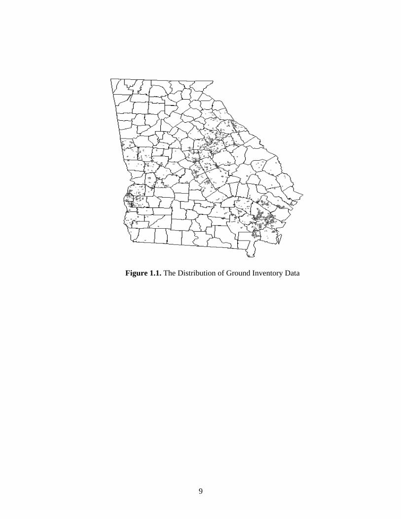
1.3.1 Ground inventory data
Ground inventory data used in this study were mostly supplied by forest industry.
Inventory variables include basal area, dominant height, forest types, timber volume, and other
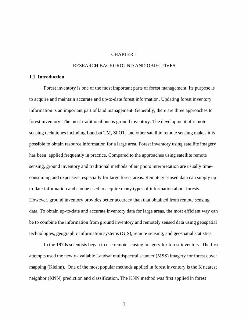
stand characteristics. Since the data is confidential, locations of ground inventory data cannot be
displayed exactly. I use Figure 1.1 to show the basic spatial pattern of the ground inventory.
1.3.2 Landsat TM data
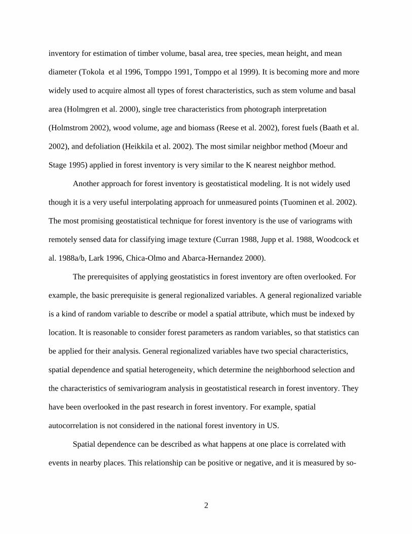
Twenty-five meter resolution Landsat TM data acquired in 2005 are used as predictors to
spatially forecast volume of trees for the whole State of Georgia. The TM imagery used is
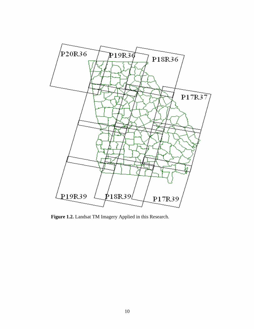
displayed in Figure 1.2 including path17 row 37, path17 row 38, path17 row 39, path18 row 36,
path18 row 37, path18 row38, path18 row39, path19 row36, path19 row37, path19 row38,
path19 row39, and path20 row36.
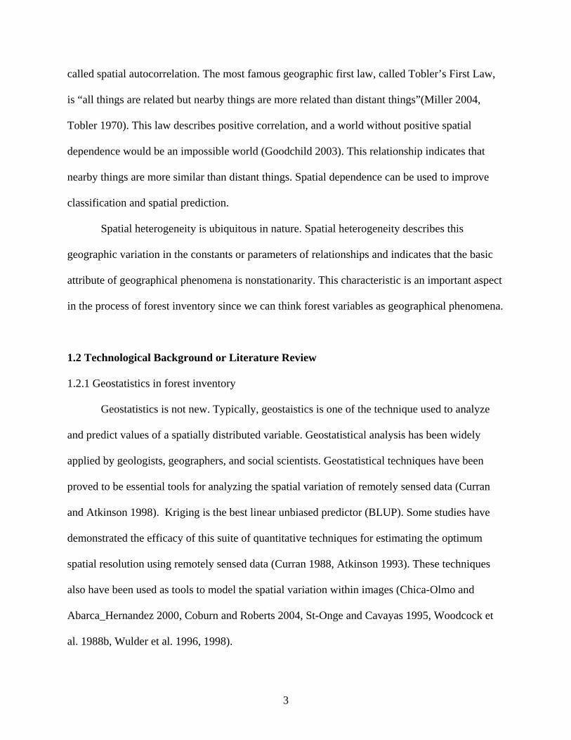
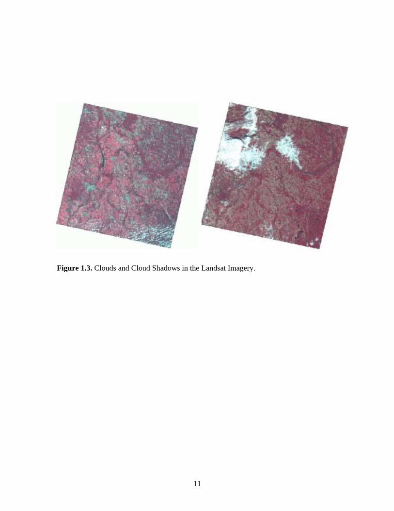
One problem with these TM data is that part of the imagery is covered with cloud and
cloud shadows (Figure 1.3). With the cloud and cloud shadows, it is impossible to predict forest
variables. I developed a nearest neighbor imputation approach to remove cloud and cloud
shadows in the images, and then used the TM data in the further steps of image analysis.
9
Figure 1.1. The Distribution of Ground Inventory Data
10
Figure 1.2. Landsat TM Imagery Applied in this Research.
11
Figure 1.3. Clouds and Cloud Shadows in the Landsat Imagery.

12
1.3.3 Other auxiliary data
The Georgia Gap Analysis Program supplied basic land cover data used as a type of
reference data in the classification process using Landsat TM imagery. The land cover data is
derived from remote sensing and modeling for general assessment of land resources (Kramer et
al 2003).
1.4 Objectives
The primary objective of this research is to achieve fine spatial resolution forest
inventory (i.e., 25-meter resolution) using the KNN imputation approach and geostatistical
approaches. Toward this end I integrate the use of remote sensing and ground inventory data. I
use the Landsat TM imagery as auxiliary data to spatially forecast forest variables of interest, but
before implementing the forecast I need to achieve three sub-objectives.
1) The traditional approach to replacing cloud and cloud shadows is (i.e., cut-and-paste)
to use cloud-free images acquired at different times. I decide not to use this approach
since every scene of satellite imagery has its individual spectral characteristics and this
traditional approach introduces an unacceptable degree of variability. I therefore need
to develop a better method to remove cloud and cloud shadows in satellite images.
2) Although the K nearest neighbor method is a popular and powerful method used for
large area forest inventory employing remotely sensed imagery, the spatial
autocorrelation and spatial dependence among the forest variables are not considered.
Kriging models, on the other hand, are developed for capturing the spatial
autocorrelation and dependence of forest variables. In addition, kriging methods are
13
the best linear unbiased predictors (BLUP) of spatial variables. I therefore develop my
own kriging-based approach for estimating fine spatial resolution forest variables.
3) The K nearest neighbor imputation has been widely applied for forest inventory, but
the disadvantages of K nearest neighbor are little explored. The two main
disadvantages are the selection of K and computation cost. The computation cost can
be partly solved using fast computation algorithms or data reduction methods. The
more important point is the selection of K, which is the number of nearest neighbors.
This number helps determine the accuracy of the forecasted variables. I therefore
explore methods of selecting K.
1.5 Methodology
1.5.1 K nearest neighbor imputation
The nearest neighbor approach is one of the most popular methods applied in GIS and
remote sensing. The basic functions based on the nearest neighbor approach are widely built into
GIS and remote sensing software, such as ArcInfo, ArcView, ERDAS Imagine, and Idrisi. The
nearest neighbor approach is also extensively applied in forest inventory. K nearest neighbor
imputation, an extension of the nearest neighbor method, is the nearest neighbor method when
K=1. Wong and Lane (1983) used the K nearest neighbor method to evaluate the most likely
number of species clusters within the population covered by their data, and discussed in detail
the procedures of statistical techniques used. Recently, K nearest neighbor imputation has also
become widely used in forest inventory as I discussed earlier. The basic steps of this method
employed in forest classification and forest inventory and the theme of K nearest neighbor can be
described as follows.
14
The Euclidean distance, dpi,p, is computed in the feature space (explanatory variable
space) from pixel p (a pixel to be predicted ) to each pixel pi whose ground truth is known (i.e.,
pixels within field plot i). Take K in the feature space nearest field plot pixels and denote the
distances from pixel p to the nearest field plot pixels by
d(p 1), p , . . . , d(pk),p, (d(p 1),p≤ · · ·≤d(pk),p ), k ~5–10.
The features (i.e., explanatory variables) are typically the original spectral values or their
functions in spectral or spatial space (Tomppo 1996). Ground variables, e.g. stand age, years
after thinning, can also be applied if the values are known for each pixel of the area to be
analyzed. Tomppo (1996) determined the weight for each pixel in order to get a better estimation
of forest inventory variables. He calculated the weight for each pixel using:
Sums of weights wi,p are calculated according to requirements. The weight of plot i in the
computation unit u yields:
Inventory results, by operation units, are computed utilizing the digital boundaries of
units and the weight coefficients (Formula 1-2) of the field sample plots estimated in the image
process. The area estimates for forestry land strata by computation units are obtained from the
estimated plot weights by the equation:
(1-1)
(1-2)
(1-3) ∑∈
=up
piui wc ,,
∑=
= k
j ppjppi
pi
dd
w
12
),(
2),(
),( 11
15
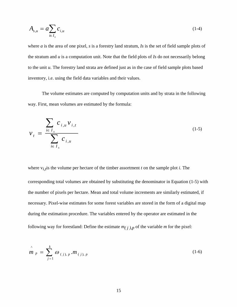
where a is the area of one pixel, s is a forestry land stratum, Is is the set of field sample plots of
the stratum and u is a computation unit. Note that the field plots of Is do not necessarily belong
to the unit u. The forestry land strata are defined just as in the case of field sample plots based
inventory, i.e. using the field data variables and their values.
The volume estimates are computed by computation units and by strata in the following
way. First, mean volumes are estimated by the formula:
where vi,tis the volume per hectare of the timber assortment t on the sample plot i. The
corresponding total volumes are obtained by substituting the denominator in Equation (1-5) with
the number of pixels per hectare. Mean and total volume increments are similarly estimated, if
necessary. Pixel-wise estimates for some forest variables are stored in the form of a digital map
during the estimation procedure. The variables entered by the operator are estimated in the
following way for forestland: Define the estimate m( j ),p of the variable m for the pixel:
(1-4)
(1-5)
(1-6) ∑=
=k
jpjpjp mm
1),(),(
^.ω
∑∑
∈
∈=
s
s
Iiui
Iitiui
t c
vcv
,
,,
∑∈
=sIi
uius caA ,,
16
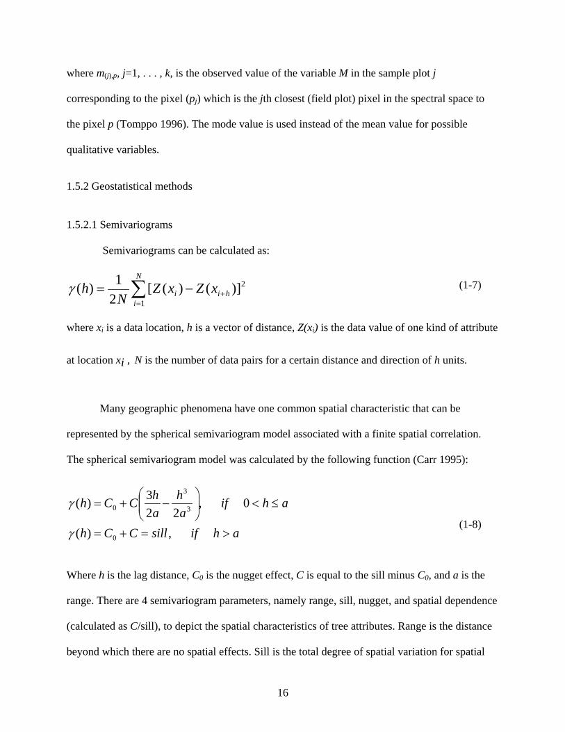
where m(j),p, j=1, . . . , k, is the observed value of the variable M in the sample plot j
corresponding to the pixel (pj) which is the jth closest (field plot) pixel in the spectral space to
the pixel p (Tomppo 1996). The mode value is used instead of the mean value for possible
qualitative variables.
1.5.2 Geostatistical methods
1.5.2.1 Semivariograms
Semivariograms can be calculated as:
where xi is a data location, h is a vector of distance, Z(xi) is the data value of one kind of attribute
at location xi , N is the number of data pairs for a certain distance and direction of h units.
Many geographic phenomena have one common spatial characteristic that can be
represented by the spherical semivariogram model associated with a finite spatial correlation.
The spherical semivariogram model was calculated by the following function (Carr 1995):
Where h is the lag distance, C0 is the nugget effect, C is equal to the sill minus C0, and a is the
range. There are 4 semivariogram parameters, namely range, sill, nugget, and spatial dependence
(calculated as C/sill), to depict the spatial characteristics of tree attributes. Range is the distance
beyond which there are no spatial effects. Sill is the total degree of spatial variation for spatial
∑=
+−=N
ihii xZxZ
Nh
1
2)]()([21)(γ (1-7)
ahifsillCCh
ahifa
hahCCh
>=+=
≤<
−+=
,)(
0,22
3)(
0
3
3
0
γ
γ
(1-8)
17
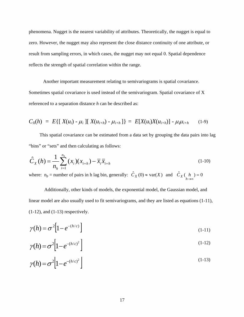
phenomena. Nugget is the nearest variability of attributes. Theoretically, the nugget is equal to
zero. However, the nugget may also represent the close distance continuity of one attribute, or
result from sampling errors, in which cases, the nugget may not equal 0. Spatial dependence
reflects the strength of spatial correlation within the range.
Another important measurement relating to semivariograms is spatial covariance.
Sometimes spatial covariance is used instead of the semivariogram. Spatial covariance of X
referenced to a separation distance h can be described as:
CX(h) = E{[ X(ui) - µi ][ X(ui+h) - µi+h ]} = E[X(ui)X(ui+h)] - µiµi+h
This spatial covariance can be estimated from a data set by grouping the data pairs into lag
“bins” or “sets” and then calculating as follows:
where: np = number of pairs in h lag bin, generally: )var()0(ˆ XCX ≈ and 0)(ˆ =
∞→hX hC
Additionally, other kinds of models, the exponential model, the Gaussian model, and
linear model are also usually used to fit semivariograms, and they are listed as equations (1-11),
(1-12), and (1-13) respectively.
(1-9)
(1-10)
(1-11)
(1-12)
(1-13)
hii
n
ihii
hX xxxx
nhC
h
+=
+ −= ∑1
))((1)(ˆ
[ ])/(2 1)( cheh −−=σγ
[ ]2)/(2 1)( cheh −−=σγ
[ ]2)/(2 1)( cheh −−=σγ
18
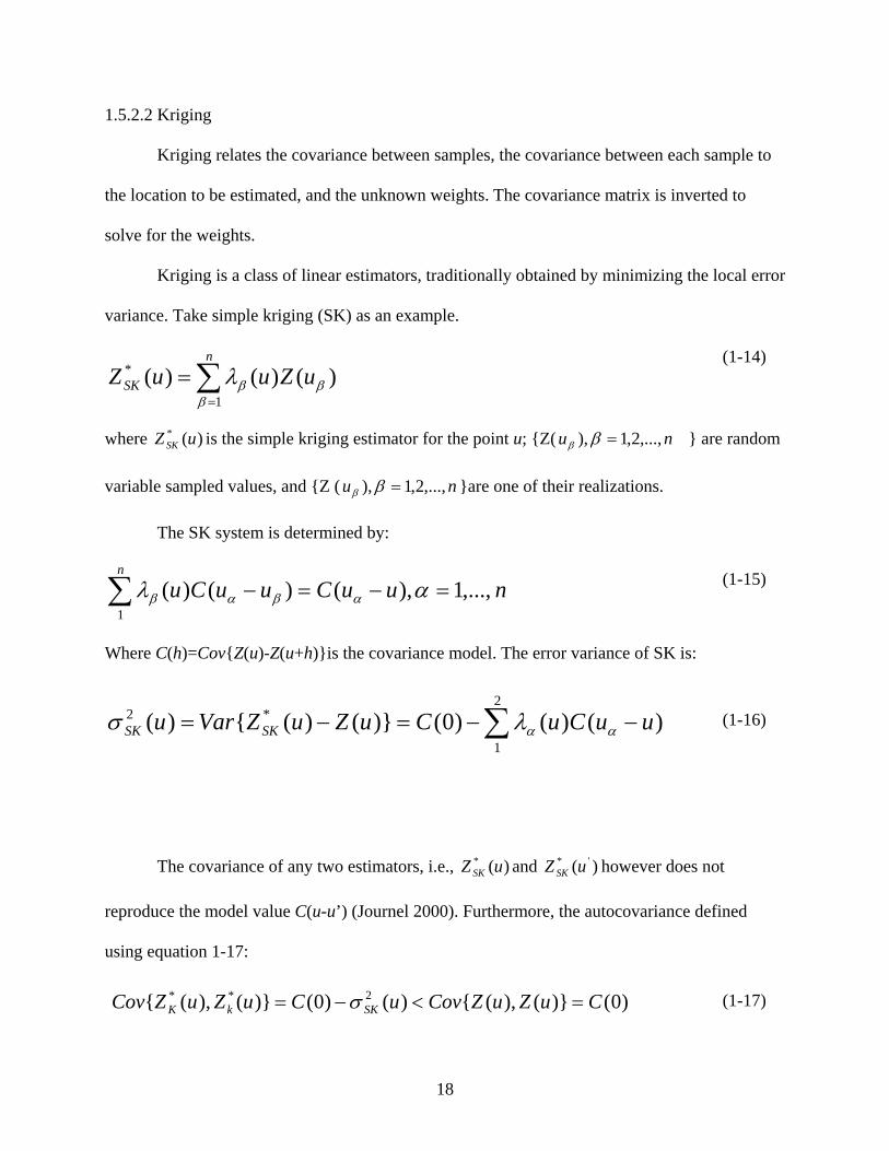
1.5.2.2 Kriging
Kriging relates the covariance between samples, the covariance between each sample to
the location to be estimated, and the unknown weights. The covariance matrix is inverted to
solve for the weights.
Kriging is a class of linear estimators, traditionally obtained by minimizing the local error
variance. Take simple kriging (SK) as an example.
where )(* uZ SK is the simple kriging estimator for the point u; {Z( nu ,...,2,1), =ββ } are random
variable sampled values, and {Z ( nu ,...,2,1), =ββ }are one of their realizations.
The SK system is determined by:
Where C(h)=Cov{Z(u)-Z(u+h)}is the covariance model. The error variance of SK is:
The covariance of any two estimators, i.e., )(* uZ SK and )( '* uZ SK however does not
reproduce the model value C(u-u’) (Journel 2000). Furthermore, the autocovariance defined
using equation 1-17:
∑=
=n
SK uZuuZ1
* )()()(β
ββλ
∑ =−=−n
nuuCuuCu1
,...,1),()()( αλ αβαβ
∑ −−=−=2
1
*2 )()()0()}()({)( uuCuCuZuZVaru SKSK ααλσ
(1-14)
(1-15)
(1-16)
(1-17) )0()}(),({)()0()}(),({ 2** CuZuZCovuCuZuZCov SKkK =<−= σ
19
is smaller than the model variance C(0). A map estimated by the kriging interpolator is always
smoothed, which is the well-known smoothing effect. Additionally, when the value for a point,
such as point u, is estimated, the kriging method does not take into consideration the estimated
values of any of the other points. Therefore, kriging is not directly used for mapping the spatial
distribution of an attribute. It is used, however, for building conditional distributions for
stochastic simulations.
In this study, I also try to use cokriging and regression kriging. They are applied in those
cases when other, usually more abundantly sampled data, can be used to help in the predictions.
Such data are called auxiliary data (as opposed to primary data) and I can assume they are
correlated with the primary data. In such situations, you can try cokriging and regression kriging
approaches, but generally the results from cokriging and regression kriging are not as smooth as
those without using auxiliary variables. To perform cokriging and regression kriging, one needs
to model not only the variograms of the auxiliary and primary data, but also the cross-variograms
between the primary and auxiliary data.
1.5.3 Remote Sensing and GIScience
Both remote sensing and GIS technologies are extensively applied in this research. For
example, unsupervised ISODATA (Iterative Self-Organizing Data Analysis Techniques)
classification is applied in order to obtain the optimal classes, and then supervised classification
is conducted to obtain hardwood and softwood classes using Landsat TM imagery. Based on
ground inventory data and remote sensing imagery, I process the massive dataset using GIS and
remote sensing software including ArcGIS 9.1 and Leica-Geosystems ERDAS Imagine and
statistical software (i.e., SAS, Splus, and R-programming). The main process technologies
include GIS data combination, projection and re-projection, transformation, extraction, mosaic,

20
subset, and mapping. The geostatistical models and nearest neighbor/K nearest neighbor methods
are implemented using SAS, Splus, and R-programming.
1.6 Chapter Organization
My dissertation is objective-oriented and problem-oriented. In other words, I designed
one approach using the weighted K nearest neighbor method and one approach using the
systematic geostatistical modeling. In both approaches I use Landsat TM imagery to achieve the
primary objective, i.e., fine-spatial-resolution forest inventory for the state of Georgia. I four
important points in this dissertation: cloud and cloud shadow removal in the TM data, i.e., the
problem in the remote sensing data source; the problems in K nearest neighbor imputation
methods; the development of the systematic geostatistical approach; and the use of the weighted
K nearest neighbor method to forecast volume of trees in Georgia.
I describe concisely the background, the data sources, the objectives, and the
methodologies in Chapter 1. In Chapter 2, I first review the literature relating to cloud and cloud
shadow removal in remote sensing data, and then develop a simple and powerful nearest
neighbor method approach to remove cloud and cloud shadows in Landsat images. In Chapter 3,
I explore the two disadvantages of the K nearest neighbor method using remote sensing data for
forest inventory after reviewing the applications of this method in forestry. In Chapter 4, I
develop a systematic geostatistical forest inventory approach using remotely sensed data. I
discuss four types of kriging methods including ordinary kriging, universal kriging, cokriging
and regression kriging using remote sensing data as auxiliary data. In Chapter 5, I use the
weighted K nearest neighbor method to forecast volume of trees using a cell size of 25-meter for
the state of Georgia. Using the mean volume of hardwood/softwood estimated by the USDA

21
Forest Inventory and Analysis Program (FIA) as the objective, I adjust my estimations to the cell
size level and obtain the unbiased estimation of hardwood/softwood volume. Then, I summarize
these estimations at the county level.
Finally, I summarize this research in Chapter 6. I discuss the performance and
significance of my work finished in Chapter 2, 3, 4, and 5. I also talk about the limitations of this
research, and point out the further studies of this research in the future.
22
CHAPTER 2
CLOUDS AND CLOUD SHADOWS REMOVAL FROM SATELLITE IMAGERY*
2.1 Introduction
Completely cloud-free remotely sensed images are not always available, especially in
tropical, neo-tropical, or humid climates, posing complications and perhaps serious constraints to
image analysis. The average cloud coverage for the entire world is about 40% (The American
Society of Photogrammetry). It is important to study removing cloud and its shadow, because the
data of interest in the scene is under cloud, and the cloud free scene cannot be obtained at an
appropriate time. This review first summarizes three approaches applied for the removal of
clouds and their shadows from satellite images
Approaches to reduce cloud and shadow are rarely studied. Mitchell et al (1977) built a
filtering procedure to remove cloud cover in satellite imagery. Liu and Hunt (1984) followed
Michell’s research and improved this filtering procedure. However, Chanda and Majumder
(1991) did not agree on one assumption in Mitchell’s procedure, and they also pointed out that
the algorithm in the research of Liu and Hunt may not be optimum. Then, they discussed out an
iterative algorithm for removing the effect of cloud. Recently, new approaches have been
developed to removing cloud based on image fusion with additive wavelet decomposition. Song
and Civeo (2002) developed another new approach to reducing cloud and shadow from satellite
images.
* This research has been submitted to IEEE Geoscience and Remote Sensing Letters, and it is in revision now.
23
2.2 Available Methods
Although different algorithms were developed in the studies of Mitchell (1977), Liu and
Hunt (1984), Chanda and Majumder (1991), these approaches are cloud distortion models and
filtering procedures. Image-fusion-based cloud removing procedures are another approach. Song
and Civeo (2002) developed the approach of removing cloud area by pixel replacing from a
secondary image.
2.2.1 Filtering procedures
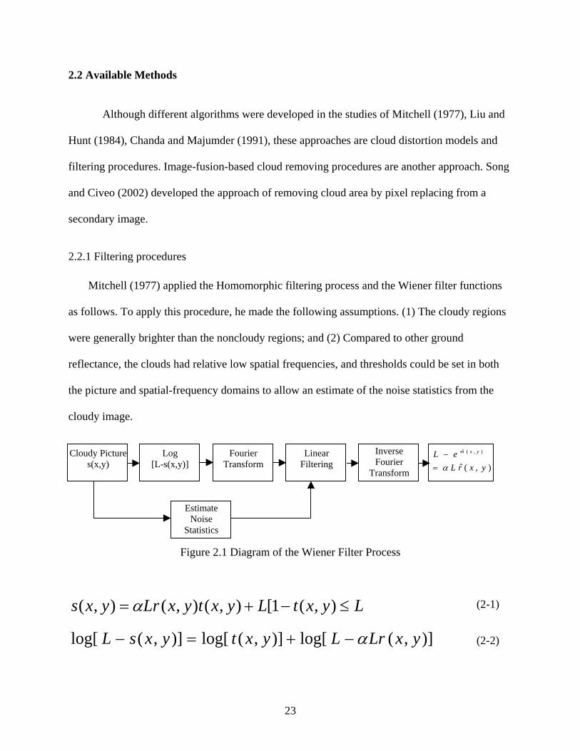
Mitchell (1977) applied the Homomorphic filtering process and the Wiener filter functions
as follows. To apply this procedure, he made the following assumptions. (1) The cloudy regions
were generally brighter than the noncloudy regions; and (2) Compared to other ground
reflectance, the clouds had relative low spatial frequencies, and thresholds could be set in both
the picture and spatial-frequency domains to allow an estimate of the noise statistics from the
cloudy image.
(2-1)
(2-2)
Cloudy Picture s(x,y)
Log [L-s(x,y)]
Fourier Transform
Linear Filtering ),(ˆ
),(ˆ
yxrLeL yxm
α=−Inverse
Fourier Transform
Estimate Noise
Statistics
Figure 2.1 Diagram of the Wiener Filter Process
LyxtLyxtyxLryxs ≤−+= ),(1[),(),(),( α
)],(log[)],(log[)],(log[ yxLrLyxtyxsL α−+=−
24
Where s(x,y) is the scanner image;
r(x,y) is the ground reflectance;
t(x,y) is the attenuation due to the cloud;
L is the sun illumination;
a is sunlight attenuation.
H(u,v) is the Wiener filter function;
SMP (u,v) is the cross power spectrum between signal and the signal plus noise;
SPP(u,v) is the power spectrum of the signal plus noise;
SNN(u,v) is the power spectrum of the noise;
Mη and Nη are the means of the signal and noise;
u and v are the two spaital frequency components;
Liu and Hunt (1984) relaxed the first assumption, because sometimes clouds are dark or
the scene is bright. Also, the Wiener filter is applicable in a stationary image field and images
with clouds are not stationary. Then, they developed a new approach (i.e., equation 2-7) to
(2-3)
(2-4)
(2-5)
(2-6)
),(),(),(
vuSvuSvuH
PP
MP=
),(),(),( vuvuSvuS NMMMMP δηη+=
),(2),(),(),( vuvuSvuSvuS NMNNMMPP δηη++=
),(),(),(),(),(
vuSvuvuSvuSvuH
PP
NMNNPP δηη−−=
25
simplify the procedure by solving equations (2-1) and (2-2), and then apply it to create the
desired image.
Chanda and Dutta Majumder (1991) agreed that the first assumption in Michell et al is
not always true, and pointed out that the results obtained with the method developed by Liu and
Hunt may not be optimum. They developed a tapered-shaped low-pass filter whose parameters
can be tuned to yield a solution of minimum errors. Shape of the filter assigned to be tapered and
circularly symmetric, because the cloud-free image of the earth surface also contains some low-
frequency components. The filter function was obtained by rearranging equation (2-2).
Where
(2-7)
(2-8)
(2-9)
(2-10)
(2-11)
),(),()],([),( 1
yxtyxsLLyxsyxLr
αα−
−=Φ= −
)],(log[)],(log[)],([ '' yxryxtyxfLog +=
),(),(),( vuRvuTvuF +=
Lyxfyxf /),(1),(' −=
),(1),(' yxryxr −=
26
2.2.2 Image fusion approach
The multi-spectral image, for example, Landsat and Spot, are applied visible, near
infrared, and infrared range. These waves cannot penetrate through clouds so the data fusion of
multi-times can compensate the lost data. The procedures include (1) multi-spectral image is
transformed to Intensity-Hue-Saturation (HIS) component in order to make histogram matching,
(2) the image is decomposed on wavelet transform, and (3) high order coefficients are combined
with the image that contained cloud for compensation the data in the hidden regions. These
procedures are relatively simple and easy to apply.
2.2.3 Song and Civeo’s Approach
Song and Civeo (2002) built a knowledge-based approach to reducing cloud and shadow.
Two date images are selected. The main image is referred to the principal image to be used for
additional analysis, and the secondary image is applied to supplement the values for cloud and
shadow regions in the main image.
This procedure includes the following parts. (1) The brightness and contrast of a
secondary image was adjusted to be the same as the main image, (2) a knowledge base is applied
to detect the presence of clouds and shadows in the main image in areas not present in the
secondary image. (3) A composite image was generated with minimal cloud and shadow by
replacing the brightness values of detected areas in the main image with those of the secondary
(2-12)
(2-13)
(3-14)
)]},('{log[),( yxfyxF ℑ=
)]},({log[),( yxtyxT ℑ=
)]},(log{[),( yxryxR ℑ=
27
image. Additionally, equation (2-15) is applied for topographical normalization. Equation (2-16)
is applied for multi-time effect brightness correction.
where DNnorm is the brightness value after normalization;
DNorig is the original brightness value;
γ is the relief values;
meanγ is the mean value of the whole relief image.
Where DNcorr is the corrected brightness of the secondary image,
DNsecd is the original brightness from the secondary image,
mainµ and mainSD is the mean and standard deviation of the main image;
dsecµ and dSDsec is the mean and standard deviation of the secondary image.
2.2.4 Discussion of available methods
Mitchell et al. (1977) developed a cloud distortion model and filtering procedures to
remove cloud cover in satellite imagery. Liu and Hunt (1984) and Chanda and Majumder (1991)
further improved the distortion model and filtering procedures. However, their methods are used
for removing thin clouds, and it is difficult to determine the range of cloud densities in which
clouds and cloud shadows (CCS) are removed efficiently.
Cihlar and Howarth (1994) and Simpson and Stitt (1998) developed special methods for
detecting and removing cloud contamination from AVHRR images. However, these methods are
not suitable for removing CCS in other satellite imagery, such as Landsat imagery. For example,
(2-15)
(2-16)
)/1(* meanorigorignorm DNDNDN γγ−+=
d
mainddmaincorr SD
SDDNDNsec
secsec *)( µµ −+=
28
one prerequisite of their methods is that there is at least one single maximum or a single
minimum for the seasonal trajectory of a satellite-derived variable.
The multi-date effect brightness correction method is another approach to removing CCS.
Song and Civco (2002) used this method to replace CCS with appropriate pixel values. This
approach is built on the sample mean and standard deviation (SD) of band values. However, the
mean and SD can only be estimated as approximations for the whole images since CCS cover
parts of the images.
2.3 Nearest Neighbor Approach
A significant obstacle to extracting information from remotely sensed imagery is the
presence of clouds and their shadows. Sometimes cloudy imagery has to be used because it is all
that is available. For example, satellite multispectral scanner imagery of the earth’s surface such
as those obtained from Landsat is often corrupted by clouds due to nadir-only observing satellites
having relatively infrequent revisiting periods.
I developed a nearest neighbor analysis (NNA) technique for replacing CCS pixels with
the most similar pixels at cloud-free areas in the same image. Nearest neighbor analysis is one
kind of popular data imputation algorithm. The technique is then applied to remove CCS
covering parts of a Landsat TM image and is then diagnostically checked.
Two satellite images covering the same area and acquired at different times are needed.
The base image is the one with relatively less CCS, and should retain the new information that is
acquired. Also, the base image is the one to be used for further applications. The other image
will be called the auxiliary image. As much as possible cloudy areas in the base image should be
cloud free in the auxiliary image. Both images are selected for this criteria based on visual
29
estimation. It is impossible to select the most similar pixels for the pixels whose signatures are
distorted by cloud and cloud shadow using only the base image, since CCS have corrupted the
real energy received and recorded by the satellite sensor. The auxiliary image is used as a
medium to determine the relationship in the base image of the most similar pixels to those pixels
whose signatures are distorted by cloud and cloud shadow.
The procedures of applying the nearest neighbor analysis technique to remove CCS in
images are depicted in Figure 2.2 The conceptions, algorithms and steps used for NNA are as
follows.
Step 1. Georegistration
The base and auxiliary satellite images often need to be geo-rectified using U.S.
Geological Survey (USGS) digital orthophoto quarter quads (DOQQs) as the sources of control
(i.e., root mean square errors should be less than 10 m). Then, the two images are registered with
each other, which also is called co-registration.
Step 2. Surface reflectance calibration
Landsat images with the spectral values being represented by digital number (DN)
contain substantial noise. To remove the solar illumination cosine effects and the topographic
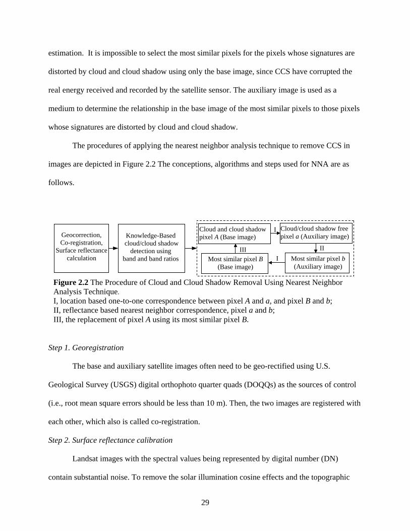
Figure 2.2 The Procedure of Cloud and Cloud Shadow Removal Using Nearest Neighbor Analysis Technique. I, location based one-to-one correspondence between pixel A and a, and pixel B and b; II, reflectance based nearest neighbor correspondence, pixel a and b; III, the replacement of pixel A using its most similar pixel B.
I Cloud and cloud shadow pixel A (Base image)
Most similar pixel b (Auxiliary image)
I II
Cloud/cloud shadow free pixel a (Auxiliary image)
Most similar pixel B (Base image)
III
Geocorrection, Co-registration,
Surface reflectance calculation
Knowledge-Based cloud/cloud shadow
detection using band and band ratios
30
effects, the algorithms developed by Chander and Markham (2003) are applied to transform DN
to radiance. I then use the available atmospheric correction package FLAASH to derive the
surface reflectance from these images more consistently.
Step 3. Knowledge-based CCSs detection
Using the relationship of location based one-to-one correspondence I determine and record,
in ascii tables, CCS areas in the base image that are cloud- and cloud-shadow free in the
auxiliary image.
For Landsat TM imagery the bands 1, 3, 4 and 6 were indicated as the best for the
detection of clouds and cloud shadows respectively. The threshold of band 1 should be greater
than a value of 5500 for dense clouds in the base image. The thin clouds are generally with in the
range (10000, 11300) of band 6. The values of these thresholds might vary for images acquired
at different times. Band 3 and 4 were used for checking cloud shadows in the base image with
band 3 less than 600 and the ratio of band 4 to band 3 bigger than 1.5. Cloud shadows and water
areas might have similar reflectance values in band 4. However shadow areas generally have
much higher values in band 4 than those in band 3, while water areas have relatively close values
in band 4 and band 3. The ratio of band 4 to band 3 therefore is used for detecting cloud
shadows.
Step 4 Nearest neighbor analysis
Nearest neighbor analysis examines the distances between each point and the closest
point to it. In an image, if pixel j has the closest surface reflectance value to that of pixel i, then, j
is called the nearest neighbor to pixel i (i.e., pixels i and j are more similar to each other than to
any other pixels in the image). Similarly, based on the surface reflectance, the most similar pixel
b in the auxiliary image can be identified for a given pixel a, in the auxiliary image. In other
31
words, the nearest neighbor algorithm determines the most similar pixels for all the
corresponding pixels identified in step 3 in the auxiliary image. The relationship of the most
similar pixels a and b in the auxiliary image can be called reflectance based nearest neighbor
correspondence.
The distance from pixel to pixel measured in reflectance is a type of point-to-point
distance. The smaller the distances are between pixels, the more similar the pixels are. Two
pixels are identical to each other if the distance between them is 0. Euclidian distance (ED) is
used in this nearest neighbor analysis technique since ED is widely applied in image processing
and classification.
where D is the Euclidian Distance between pixels i and j, L indicates satellite bands, and n is the
number of bands for the satellite imagery being used, such as n =7 for Landsat TM.
Step5 Transfer of reflectance based nearest neighbor correspondence
When the relationship of reflectance based nearest neighbor correspondence is built for
pixels in the auxiliary image, it is transferred to the base image to match the cloud-free and
cloud-shadow-free pixels in the base image to those pixels covered by CCS in the base image.
For example, suppose pixel A is covered with CCS. Pixel A in the base image and pixel a in the
auxiliary image are in location based one-to-one correspondence; likewise, pixel B in the base
image and b in the auxiliary image. Pixels A and B should be in reflectance based nearest
neighbor correspondence in the base image because pixels a and b are in reflectance based
nearest neighbor correspondence in the auxiliary image. I can therefore use the reflectance values
of pixel B to replace the reflectance of pixel A.
(2-17) ∑=
−=n
LLL jiD
1
2)(
32
Step 6 Compose an image in which clouds and cloud shadows have been removed
At last, an image in which CCS has been removed can be composed for the base image
using remote sensing software. Filtering functions need to be applied to obtain a smooth view of
the composed image.
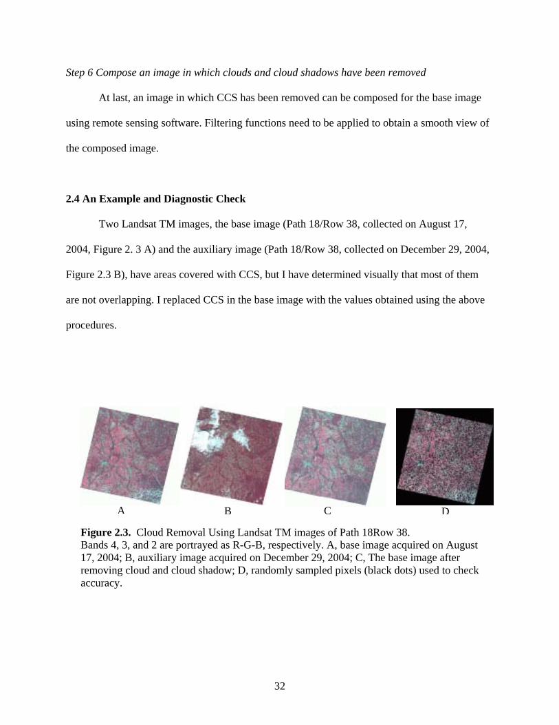
2.4 An Example and Diagnostic Check
Two Landsat TM images, the base image (Path 18/Row 38, collected on August 17,
2004, Figure 2. 3 A) and the auxiliary image (Path 18/Row 38, collected on December 29, 2004,
Figure 2.3 B), have areas covered with CCS, but I have determined visually that most of them
are not overlapping. I replaced CCS in the base image with the values obtained using the above
procedures.
Figure 2.3. Cloud Removal Using Landsat TM images of Path 18Row 38. Bands 4, 3, and 2 are portrayed as R-G-B, respectively. A, base image acquired on August 17, 2004; B, auxiliary image acquired on December 29, 2004; C, The base image after removing cloud and cloud shadow; D, randomly sampled pixels (black dots) used to check accuracy.
C BA D
33
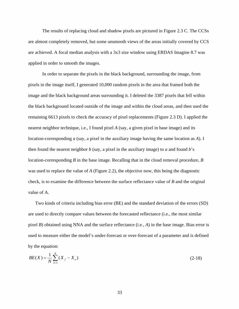
The results of replacing cloud and shadow pixels are pictured in Figure 2.3 C. The CCSs
are almost completely removed, but some unsmooth views of the areas initially covered by CCS
are achieved. A focal median analysis with a 3x3 size window using ERDAS Imagine 8.7 was
applied in order to smooth the images.
In order to separate the pixels in the black background, surrounding the image, from
pixels in the image itself, I generated 10,000 random pixels in the area that framed both the
image and the black background areas surrounding it. I deleted the 3387 pixels that fell within
the black background located outside of the image and within the cloud areas, and then used the
remaining 6613 pixels to check the accuracy of pixel replacements (Figure 2.3 D). I applied the
nearest neighbor technique, i.e., I found pixel A (say, a given pixel in base image) and its
location-corresponding a (say, a pixel in the auxiliary image having the same location as A). I
then found the nearest neighbor b (say, a pixel in the auxiliary image) to a and found b’s
location-corresponding B in the base image. Recalling that in the cloud removal procedure, B
was used to replace the value of A (Figure 2.2), the objective now, this being the diagnostic
check, is to examine the difference between the surface reflectance value of B and the original
value of A.
Two kinds of criteria including bias error (BE) and the standard deviation of the errors (SD)
are used to directly compare values between the forecasted reflectance (i.e., the most similar
pixel B) obtained using NNA and the surface reflectance (i.e., A) in the base image. Bias error is
used to measure either the model’s under-forecast or over-forecast of a parameter and is defined
by the equation:
)(1)(1
o
N
nf XX
NXBE −= ∑
=(2-18)
34
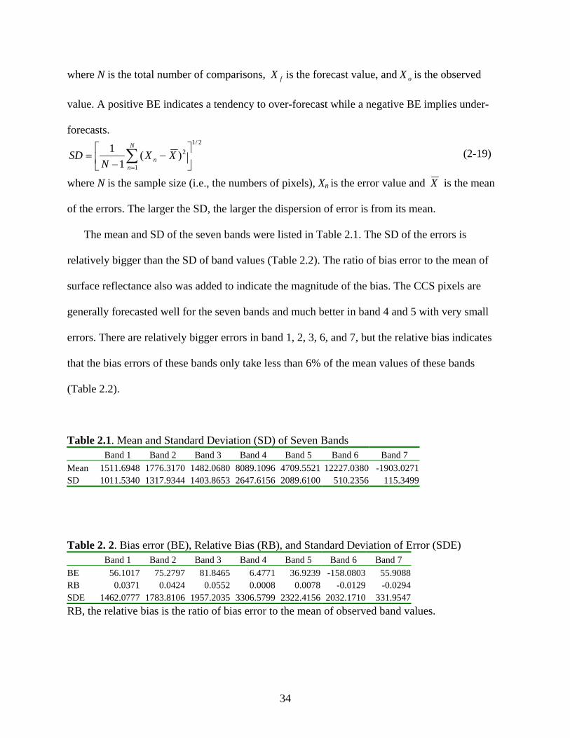
where N is the total number of comparisons, fX is the forecast value, and oX is the observed
value. A positive BE indicates a tendency to over-forecast while a negative BE implies under-
forecasts.
where N is the sample size (i.e., the numbers of pixels), Xn is the error value and X is the mean
of the errors. The larger the SD, the larger the dispersion of error is from its mean.
The mean and SD of the seven bands were listed in Table 2.1. The SD of the errors is
relatively bigger than the SD of band values (Table 2.2). The ratio of bias error to the mean of
surface reflectance also was added to indicate the magnitude of the bias. The CCS pixels are
generally forecasted well for the seven bands and much better in band 4 and 5 with very small
errors. There are relatively bigger errors in band 1, 2, 3, 6, and 7, but the relative bias indicates
that the bias errors of these bands only take less than 6% of the mean values of these bands
(Table 2.2).
Table 2.1. Mean and Standard Deviation (SD) of Seven Bands Band 1 Band 2 Band 3 Band 4 Band 5 Band 6 Band 7 Mean 1511.6948 1776.3170 1482.0680 8089.1096 4709.5521 12227.0380 -1903.0271 SD 1011.5340 1317.9344 1403.8653 2647.6156 2089.6100 510.2356 115.3499
Table 2. 2. Bias error (BE), Relative Bias (RB), and Standard Deviation of Error (SDE) Band 1 Band 2 Band 3 Band 4 Band 5 Band 6 Band 7 BE 56.1017 75.2797 81.8465 6.4771 36.9239 -158.0803 55.9088 RB 0.0371 0.0424 0.0552 0.0008 0.0078 -0.0129 -0.0294 SDE 1462.0777 1783.8106 1957.2035 3306.5799 2322.4156 2032.1710 331.9547 RB, the relative bias is the ratio of bias error to the mean of observed band values.
2/1
1
2)(1
1
−
−= ∑
=
N
nn XX
NSD (2-19)

35
2.5 Conclusions
A nearest neighbor analysis technique has been developed and conducted in order to
remove CCS, and compose a remotely sensed image with very few CCSs. The example and
diagnostic check indicate that the NNA technique is an efficient approach. It is simple and easy
to understand and practice. The CCS were almost completely removed in the example using
Landsat image Path 18/Row 38. An additional image acquired at a different time can be used
again to remove CCS if there are overlaps of CCS in the base and auxiliary images. The nearest
neighbor analysis also can be used to remove CCS for other satellite images other than Landsat.
The reflectance based nearest neighbor correspondence in the base image and auxiliary
image should be the same or very similar. The two images cover the same area, were obtained
using the same remote sensor, and have been processed using the same procedures.
The threshold of band 1 is used for detecting clouds. The threshold of band 4 and the
ratio 2 of band 4 to band 3 are used to distinguish cloud shadows in satellite imagery. The ratio
improved the discrimination between cloud shadows and water areas. The three criteria are
flexible and adjustable from image to image.
The nearest neighbor analysis technique is a simple and efficient method to remove CCS
from satellite imagery. Another advantage of NNA is that its efficiency (i.e., the accuracy of
removing clouds and cloud shadows) can be diagnostically checked as it is applied. The errors
and the standard deviations of errors in forecasting band values indicate whether some of them
could be used for further applications. It is unwise to use the forecasting band values for further
applications when big errors and standard deviations of errors exist.
36
CHAPTER 3
K NEAREST NEIGHBOR METHOD
FOR FOREST INVENTORY USING REMOTE SENSING DATA∗ 3.1 Introduction
The K nearest neighbor (KNN) method of image analysis is practical, relatively easy to
implement, and is becoming one of the most popular methods for conducting forest inventory
using remote sensing data. The KNN is often named K nearest neighbor classifier when it is used
for classifying categorical variables, while KNN is called K nearest neighbor regression when it
is applied for predicting non-categorical variables. As an instance-based estimation method,
KNN has two problems: the selection of K values and computation cost. We address the
problems of K selection by applying a new approach, which is the combination of the
Kolmogorov-Smirnov (KS) test and cumulative distribution function (CDF) to determine the
optimal K. Our research indicates that the KS tests and CDF are much more efficient for
selecting K than cross validation and bootstrapping, which are more commonly used today. We
use remote sensing data reduction techniques—such as principal component analysis, layer
combination, and computation of a vegetation index—to save computation cost. We also
consider the theoretical and practical implications of different K values in forest inventory.
∗ This research has been submitted to GIScience and Remote Sensing. Now it is in revision.
37
The K nearest neighbor (KNN) method of image analysis is widely used in the estimation of
single tree characteristics and stand attributes, and its algorithm and procedures are discussed in
a number of studies (Fazakas and Nilsson, 1996; Holmstrom, 2002; Katila et al. 2000; Katila and
Tomppo, 2001; Tokola, 2000; Tokola, et al. 1996; Tomppo, 1991; Tomppo and Halme 2004; and
Trotter, et al., 1997). The KNN method has two advantages in that it uses a nonparametric
approach and allows for the use of robust to noisy training data. It is therefore becoming one of
the most popular methods applied for forest inventory using large-area remote sensing data.
Tomppo et al. (1999), Franco-Lopez and Bauer (2001), and Trotter, et al. (1997) reported using
the KNN technique to classify satellite image data for large areas. Tomppo (1991) and other
researchers first applied the KNN method for forest classification and forest inventory.
As a kind of instance-based data mining approach it still has two problems: the selection of
K values and computation cost (James 1985). The two problems are little discussed although a
great number of studies of KNN using remote sensing data are available. Computation cost
results from the distance computation of each query instance to all training samples. Hardin and
Thomson (1992) explore a fast nearest neighbor classification approach using a k-d tree and
partially solved the problem of computation cost, but remote sensing data reduction is still
important when a large dataset is applied. Jensen (1986) discusses in detail the methods of band
reduction and selection. We discuss and then apply remote sensing data reduction in this paper in
order to partially resolve the disadvantage of computation cost. The reduction techniques might
include determining an optimal combination of bands, performing principal component analysis
38
(PCA) of multi-bands, and calculating a vegetation index, all three of which can reduce data size
significantly while keeping almost all the useful information in the original data.
We explore the problem of the selection of K in the context of KNN being used for spatial
prediction using remotely sensed imagery. KNN predictions are based on the intuitive
assumption that objects close in distance (say, vector space) are potentially similar. It is an
extension of the nearest neighbor method, which is widely used in image processing and
classification. KNN methods are applied not only for grand mean estimation, but also for spatial
prediction. The bigger the K values, the closer is the estimation to the mean of a forest variable,
but as K grows we lose variability in the field data. The smaller the K values, the more the
estimation is able to maintain the variation in the field data.
Several important points relating to the selection of K must be considered. For example,
what values of K result in estimations retaining the range of variability present in the field data?
Also, does a relatively larger standard deviation indicate the estimations significantly cover the
variability in the field data? Compared with the field data, are the estimations using different K
values significantly different from each other?
KNN is used not only for grand mean estimation of forest stand characteristics but also for
spatial estimation and classification of spatial characteristics of forests (e.g.,
fine-spatial-resolution estimation of basal area, timber volume, species, age, mortality, etc.),
providing important information for forest management. It is the selection of K that determines
the accuracy of the predictions in forest inventory. In order to resolve the above questions, the
selection of K must be answered; i.e., how big or how small of a K value is an optimal selection?
39
3.2 Objectives
The objectives of this research include the following:
(1) We discuss the available K selection methods and we explore the shortcomings of
root mean square error (RMSE) and re-sampling statistics for K selection.
(2) For selecting K for forest inventory applications we use a new approach, which is a
combination of the Kolmogorov-Smirnov (KS) test and cumulative distribution
functions (CDF). We determine that when using this combination, the estimates of
forest variables obtained from KNN will have the same or similar distribution as the
observed samples. We also discuss other advantages of the KS test and CDF for
selecting K.
(3) We discuss principal component analysis and normalized difference vegetation index,
which are both data reduction techniques for remote sensing to save computation
cost.
3.3 Study Area and data sources
The study area is Marion County located in southwestern Georgia (Fig. 1). The test area is
relatively flat terrain and the vegetation is uneven-aged coniferous stands with the dominant
species being Loblolly pine (Pinus taeda). The range of average monthly temperatures is from
35º F to 90º F, and the range of average monthly precipitation is from 5.842 to 14.224 cm.
A private timber company inventoried the ground data in September 1999. The plot size was
30.5×30.5 m (100×100 ft) and the location of each plot was archived by differential Global

40
Positioning System (GPS) techniques with an accuracy of approximately±5 m. The total 128
plots are mapped in UTM zone 17 (black polygons in Fig. 1). Within each plot, basal area and
tree height were measured and used to estimate volume. In this research only basal area was used
as ground truth data to evaluate the predicted basal area from Landsat ETM+ data, path19 row37,
acquired on September 10, 1999.
The image of the Marion County region was a subset from the ETM+ scene path19 row37
after georectification using U.S. Geological Survey (USGS) digital orthophoto quarterquads
(DOQQs) as the sources of control (RMSE less than 10 m). This resulted in a 6-band (band 1~5
and 7) image for the KNN analysis. Three types of data — two principal component layers
(PCA), a normalized difference of vegetation index (NDVI) image, and the combination of two
principal component layers and the NDVI image (NDVIPCA)— were derived using band
Figure 3.1. The Study Area Is Marion County, Georgia. Groundinventoried plots are indicated as black polygons superimposed on amosaic of Landsat images.
41
reduction and transformation methods. The Landsat image and ground data associated with GPS
point locations had been projected in UTM zone17. We overlaid the GPS and ground data on the
image and then attached the nearest pixel values of Landsat images including the 6 band data,
PCA, NDVI and NDVIPCA to the ground inventory data using ArcInfo grid functions. Then we
applied the KNN methods to estimate the basal area.
3.4 Methodology
3.4.1 KNN Algorithms
Our KNN algorithm that is memory-based and has been widely used for data mining
requires no model to be fit (Hastie et al. 2001). This algorithm can be depicted as follows: given
a query point xi, we need to find the K training points xj, j = 1, 2, …, k, closest in distance to xi .
For categorical variables we then classify xi using the majority vote among the K neighbors. For
non-categorical variables, we predict xi calculating an average or weighted average of the K
neighbors. The KNN is often named K nearest neighbor classifier when it is used for classifying
categorical variables, while KNN is called K nearest neighbor regression when it is applied for
predicting non-categorical variables.
In using the KNN algorithm as a procedure for forest inventory, if the objective of our
research is to obtain a value of basal area of a pixel i (a plot or stand), this KNN algorithm will
find K other pixels that have basal area values and that also have the most similar spectral values
(we use Euclidian distance as the measure of spectral difference between pixels) to pixel i in the
multispectral imagery. Then, an average value of basal area from the K other pixels is used as a
42
prediction for pixel i.
The selection of values of K is essential to accurately use KNN to analyze remote sensing
data for forest inventory. Generally, the results of using a particular K are evaluated by
examining prediction errors, which can be done in several ways. For example, direct calculation
of RMSE is commonly used to evaluate the prediction results of different Ks (Katila and Tomppo,
2001; McRoberts et al., 2002; Tomppo, et al., 2002). Re-sampling statistics such as leave-one-out
cross validation and bootstrapping (Franco-Lopez et al. 2001; Katila and Tomppo, 2001 and
2002; Trotter, et al., 1997) also are applied to evaluate the results of different K’s.
In this paper, we developed a new approach for selecting K, wherein the choice of K is
based on the combination of the Kolmogorov-Smirnov (KS) test and cumulative distribution
functions (CDF). The KS test is a powerful evaluation that is generally used to determine
whether two data samples are compatible. We use it here to determine the significance of the
difference between the estimation and sample data. Displays of the empirical CDF can be used to
check whether the predictions based on different Ks have the same or similar distributions as the
sample data.
3.4.2 Direct Calculations of RMSE and Comparisons of Mean and SD
The RMSE and the mean and standard deviation (SD) of basal area were examined using
equations (3-1), (3-2), and (3-3) in the evaluation of the results of different K.
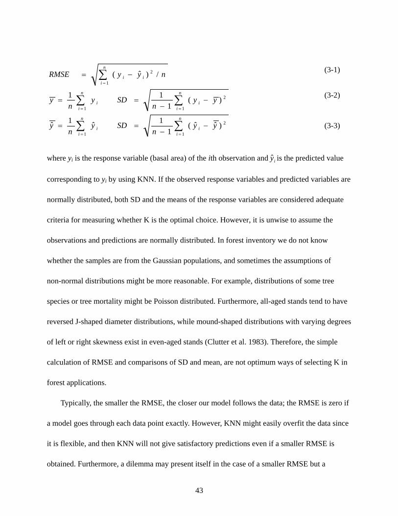
43
where yi is the response variable (basal area) of the ith observation and iy is the predicted value
corresponding to yi by using KNN. If the observed response variables and predicted variables are
normally distributed, both SD and the means of the response variables are considered adequate
criteria for measuring whether K is the optimal choice. However, it is unwise to assume the
observations and predictions are normally distributed. In forest inventory we do not know
whether the samples are from the Gaussian populations, and sometimes the assumptions of
non-normal distributions might be more reasonable. For example, distributions of some tree
species or tree mortality might be Poisson distributed. Furthermore, all-aged stands tend to have
reversed J-shaped diameter distributions, while mound-shaped distributions with varying degrees
of left or right skewness exist in even-aged stands (Clutter et al. 1983). Therefore, the simple
calculation of RMSE and comparisons of SD and mean, are not optimum ways of selecting K in
forest applications.
Typically, the smaller the RMSE, the closer our model follows the data; the RMSE is zero if
a model goes through each data point exactly. However, KNN might easily overfit the data since
it is flexible, and then KNN will not give satisfactory predictions even if a smaller RMSE is
obtained. Furthermore, a dilemma may present itself in the case of a smaller RMSE but a
)3()ˆˆ(1
1ˆ1ˆ
)2()(1
11
)1(/)ˆ(
1
2
1
1
2
1
1
2
∑∑
∑∑
∑
==
==
=
−−
==
−−
==
−=
n
ii
n
ii
n
ii
n
ii
n
iii
yyn
SDyn
y
yyn
SDyn
y
nyyRMSE (3-1)
(3-2)
(3-3)
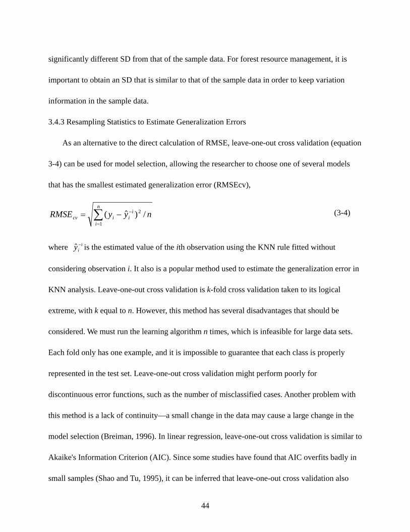
44
significantly different SD from that of the sample data. For forest resource management, it is
important to obtain an SD that is similar to that of the sample data in order to keep variation
information in the sample data.
3.4.3 Resampling Statistics to Estimate Generalization Errors
As an alternative to the direct calculation of RMSE, leave-one-out cross validation (equation
3-4) can be used for model selection, allowing the researcher to choose one of several models
that has the smallest estimated generalization error (RMSEcv),
where iiy −ˆ is the estimated value of the ith observation using the KNN rule fitted without
considering observation i. It also is a popular method used to estimate the generalization error in
KNN analysis. Leave-one-out cross validation is k-fold cross validation taken to its logical
extreme, with k equal to n. However, this method has several disadvantages that should be
considered. We must run the learning algorithm n times, which is infeasible for large data sets.
Each fold only has one example, and it is impossible to guarantee that each class is properly
represented in the test set. Leave-one-out cross validation might perform poorly for
discontinuous error functions, such as the number of misclassified cases. Another problem with
this method is a lack of continuity—a small change in the data may cause a large change in the
model selection (Breiman, 1996). In linear regression, leave-one-out cross validation is similar to
Akaike's Information Criterion (AIC). Since some studies have found that AIC overfits badly in
small samples (Shao and Tu, 1995), it can be inferred that leave-one-out cross validation also
∑=
−−=n
i
iiicv nyyRMSE
1
2 /)ˆ( (3-4)
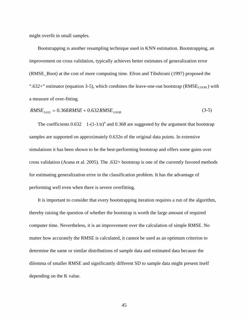
45
might overfit in small samples.
Bootstrapping is another resampling technique used in KNN estimation. Bootstrapping, an
improvement on cross validation, typically achieves better estimates of generalization error
(RMSE_Boot) at the cost of more computing time. Efron and Tibshirani (1997) proposed the
“.632+” estimator (equation 3-5), which combines the leave-one-out bootstrap (RMSELOOB ) with
a measure of over-fitting.
The coefficients 0.632≈1-(1-1/n)n and 0.368 are suggested by the argument that bootstrap
samples are supported on approximately 0.632n of the original data points. In extensive
simulations it has been shown to be the best-performing bootstrap and offers some gains over
cross validation (Arana et al. 2005). The .632+ bootstrap is one of the currently favored methods
for estimating generalization error in the classification problem. It has the advantage of
performing well even when there is severe overfitting.
It is important to consider that every bootstrapping iteration requires a run of the algorithm,
thereby raising the question of whether the bootstrap is worth the large amount of required
computer time. Nevertheless, it is an improvement over the calculation of simple RMSE. No
matter how accurately the RMSE is calculated, it cannot be used as an optimum criterion to
determine the same or similar distributions of sample data and estimated data because the
dilemma of smaller RMSE and significantly different SD to sample data might present itself
depending on the K value.
LOOBRMSERMSERMSE 632.0368.0632.0 += (3-5)
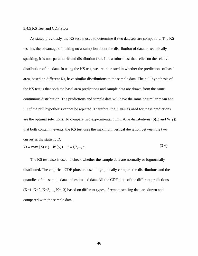
46
3.4.5 KS Test and CDF Plots
As stated previously, the KS test is used to determine if two datasets are compatible. The KS
test has the advantage of making no assumption about the distribution of data, or technically
speaking, it is non-parametric and distribution free. It is a robust test that relies on the relative
distribution of the data. In using the KS test, we are interested in whether the predictions of basal
area, based on different Ks, have similar distributions to the sample data. The null hypothesis of
the KS test is that both the basal area predictions and sample data are drawn from the same
continuous distribution. The predictions and sample data will have the same or similar mean and
SD if the null hypothesis cannot be rejected. Therefore, the K values used for these predictions
are the optimal selections. To compare two experimental cumulative distributions (S(x) and W(y))
that both contain n events, the KS test uses the maximum vertical deviation between the two
curves as the statistic D:
The KS test also is used to check whether the sample data are normally or lognormally
distributed. The empirical CDF plots are used to graphically compare the distributions and the
quantiles of the sample data and estimated data. All the CDF plots of the different predictions
(K=1, K=2, K=3,…, K=13) based on different types of remote sensing data are drawn and
compared with the sample data.
niyWxSD ii ,...,2,1|)()(|max =−= (3-6)
47
3.5 Data reduction
3.5.1 Principal Component Analysis
The principal components analysis (PCA) is a linear transformation used for data
compression. It is practical and helpful in the remote sensing realm because sometimes there are
redundant data in the different bands of a multispectral image. PCA reduces the dimensionality
of the dataset, compacts the data into fewer bands which are noncorrelated and independent, and
without losing significant information saves on storage space and speeds up processing. The first
few components of the PCA usually capture the majority of the information, so the number of
bands in a Landsat ETM+ image may be reduced from 7 to 2 or 3. In this research we ran PCA in
Leica Geosystems’ ERDAS Imagine using the built-in model. The first two components
explained 95% of the variation in the 6-band image.
3.5.2 Normalized Difference Vegetation Index
The Normalized Difference Vegetation Index (NDVI) image (equation 3-7) provides the
phenological "greenness" measure. It is one of many vegetation indices that can aid in
visualization of an image and can be used to monitor the health of vegetation on the ground. It
also is the most important index used to estimate volume and basal area in forest inventory. The
NDVI has an added benefit of reducing the number of bands for an image down to one.
In this research, using KNN we analyzed a 6-band Landsat ETM+ image, then a PCA image
and a NDVI image, and then finally we implemented KNN using the combined PCA and NDVI.
3434
BandBandBandBand
REDNIRREDNIRNDVI
+−
=+−
= (3-7)
48
3.6 Results
The sample data included 128 plots of loblolly pine stands for which basal area was
measured to serve as ground truth data for evaluating predicted basal area from Landsat ETM+
data. The mean basal area of observations was 25.81 m2/ha, and the standard deviation was 10.13
m2/ha. The KS test indicated that it is very unlikely that the sample was normally distributed: P=
0.04 where the normal distribution had a mean equal to 26.86 and standard deviation equal to
9.80. Furthermore, it is not likely that it was lognormally distributed: P= 0.04 where the
lognormal distribution had a geometric mean of 22.74 and a multiplicative standard deviation of
0.39. Thus, in this situation, the mean and standard deviation (SD) were not adequate indices for
selecting K.
Results of direct calculation of basal area and re-sampling statistics of estimated errors from
the 6-band image, PCA image, NDVI image, and NDVIPCA images, are summarized in Tables
3.1 to 3.4. These tables reveal that the estimated standard deviation decays quickly as K
increases. The three kinds of errors, RMSE, RMSEcv, and RMSELOOB have the same trends as
the estimated standard deviation and decrease as K increases. There is not much difference
among estimated means of basal area from K=1 to 13.
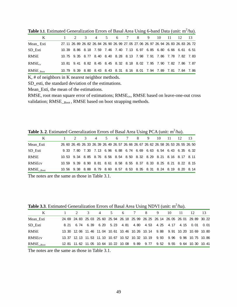
49
Table 3.1. Estimated Generalization Errors of Basal Area Using 6-band Data (unit: m2/ha). K 1 2 3 4 5 6 7 8 9 10 11 12 13
Mean_ Esti 27.11 26.89 26.82 26.84 26.90 26.99 27.05 27.06 26.97 26.94 26.83 26.83 26.72
SD_Esti 10.39 8.86 8.18 7.59 7.46 7.40 7.13 6.97 6.85 6.80 6.66 6.61 6.51
RMSE 10.75 9.35 8.77 8.40 8.40 8.28 8.13 7.98 7.91 7.86 7.78 7.82 7.83
RMSEcv 10.81 9.41 8.82 8.45 8.45 8.32 8.18 8.02 7.95 7.90 7.82 7.86 7.87
RMSE_Boot 10.79 9.39 8.80 8.43 8.43 8.31 8.16 8.01 7.94 7.89 7.81 7.84 7.86
K, # of neighbors in K nearest neighbor methods. SD_esti, the standard deviation of the estimations. Mean_Esti, the mean of the estimations. RMSE, root mean square error of estimations; RMSEcv, RMSE based on leave-one-out cross validation; RMSE_Boot , RMSE based on boot strapping methods. Table 3. 2. Estimated Generalization Errors of Basal Area Using PCA (unit: m2/ha).
K 1 2 3 4 5 6 7 8 9 10 11 12 13 Mean_Esti 26.60 26.45 26.33 26.39 26.49 26.57 26.66 26.67 26.62 26.58 26.53 26.55 26.50
SD_Esti 9.33 7.80 7.30 7.13 6.96 6.88 6.74 6.69 6.63 6.54 6.43 6.35 6.32
RMSE 10.53 9.34 8.85 8.76 8.56 8.54 8.50 8.32 8.29 8.21 8.16 8.17 8.11
RMSEcv 10.59 9.39 8.90 8.81 8.61 8.58 8.55 8.37 8.33 8.25 8.21 8.22 8.15
RMSE_Boot 10.56 9.38 8.88 8.79 8.60 8.57 8.53 8.35 8.31 8.24 8.19 8.20 8.14
The notes are the same as those in Table 3.1.
Table 3.3. Estimated Generalization Errors of Basal Area Using NDVI (unit: m2/ha). K 1 2 3 4 5 6 7 8 9 10 11 12 13
Mean_Esti 24.69 24.83 25.03 25.60 25.94 26.18 25.99 26.25 26.14 26.05 26.01 29.89 30.22
SD_Esti 8.21 6.74 6.39 6.20 5.23 4.81 4.80 4.53 4.25 4.17 4.15 0.01 0.01
RMSE 13.30 12.06 11.46 11.04 10.61 10.46 10.26 10.14 9.88 9.91 10.20 10.69 10.80
RMSEcv 13.37 12.13 11.53 11.10 10.67 10.52 10.32 10.19 9.93 9.96 9.96 10.75 10.86
RMSE_Boot 12.81 11.62 11.05 10.64 10.22 10.08 9.89 9.77 9.52 9.55 9.64 10.30 10.41
The notes are the same as those in Table 3.1.
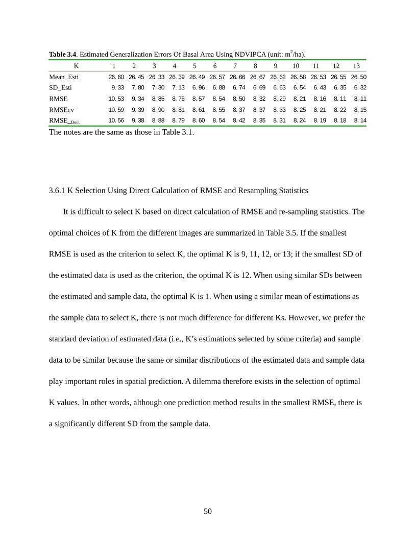
50
Table 3.4. Estimated Generalization Errors Of Basal Area Using NDVIPCA (unit: m2/ha). K 1 2 3 4 5 6 7 8 9 10 11 12 13
Mean_Esti 26.60 26.45 26.33 26.39 26.49 26.57 26.66 26.67 26.62 26.58 26.53 26.55 26.50
SD_Esti 9.33 7.80 7.30 7.13 6.96 6.88 6.74 6.69 6.63 6.54 6.43 6.35 6.32
RMSE 10.53 9.34 8.85 8.76 8.57 8.54 8.50 8.32 8.29 8.21 8.16 8.11 8.11
RMSEcv 10.59 9.39 8.90 8.81 8.61 8.55 8.37 8.37 8.33 8.25 8.21 8.22 8.15
RMSE_Boot 10.56 9.38 8.88 8.79 8.60 8.54 8.42 8.35 8.31 8.24 8.19 8.18 8.14
The notes are the same as those in Table 3.1.
3.6.1 K Selection Using Direct Calculation of RMSE and Resampling Statistics
It is difficult to select K based on direct calculation of RMSE and re-sampling statistics. The
optimal choices of K from the different images are summarized in Table 3.5. If the smallest
RMSE is used as the criterion to select K, the optimal K is 9, 11, 12, or 13; if the smallest SD of
the estimated data is used as the criterion, the optimal K is 12. When using similar SDs between
the estimated and sample data, the optimal K is 1. When using a similar mean of estimations as
the sample data to select K, there is not much difference for different Ks. However, we prefer the
standard deviation of estimated data (i.e., K’s estimations selected by some criteria) and sample
data to be similar because the same or similar distributions of the estimated data and sample data
play important roles in spatial prediction. A dilemma therefore exists in the selection of optimal
K values. In other words, although one prediction method results in the smallest RMSE, there is
a significantly different SD from the sample data.
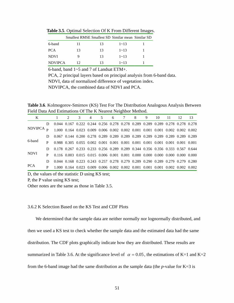
51
Table 3.5. Optimal Selection Of K From Different Images. Smallest RMSE Smallest SD Similar mean Similar SD
6-band 11 13 1~13 1 PCA 13 13 1~13 1 NDVI 9 13 1~13 1 NDVIPCA 12 13 1~13 1
6-band, band 1~5 and 7 of Landsat ETM+. PCA, 2 principal layers based on principal analysis from 6-band data. NDVI, data of normalized difference of vegetation index. NDVIPCA, the combined data of NDVI and PCA.
Table 3.6. Kolmogorov-Smirnov (KS) Test For The Distribution Analogous Analysis Between Field Data And Estimations Of The K Nearest Neighbor Method.
K 1 2 3 4 5 6 7 8 9 10 11 12 13 D 0.044 0.167 0.222 0.244 0.256 0.278 0.278 0.289 0.289 0.289 0.278 0.278 0.278
NDVIPCA P 1.000 0.164 0.023 0.009 0.006 0.002 0.002 0.001 0.001 0.001 0.002 0.002 0.002D 0.067 0.144 0.200 0.278 0.289 0.289 0.289 0.289 0.289 0.289 0.289 0.289 0.289
6-band P 0.988 0.305 0.055 0.002 0.001 0.001 0.001 0.001 0.001 0.001 0.001 0.001 0.001D 0.178 0.267 0.233 0.233 0.256 0.289 0.289 0.344 0.356 0.356 0.333 0.567 0.644
NDVI P 0.116 0.003 0.015 0.015 0.006 0.001 0.001 0.000 0.000 0.000 0.000 0.000 0.000D 0.044 0.168 0.223 0.243 0.257 0.278 0.279 0.289 0.290 0.289 0.279 0.279 0.280
PCA P 1.000 0.164 0.023 0.009 0.006 0.002 0.002 0.001 0.001 0.001 0.002 0.002 0.002
D, the values of the statistic D using KS test; P, the P value using KS test; Other notes are the same as those in Table 3.5.
3.6.2 K Selection Based on the KS Test and CDF Plots
We determined that the sample data are neither normally nor lognormally distributed, and
then we used a KS test to check whether the sample data and the estimated data had the same
distribution. The CDF plots graphically indicate how they are distributed. These results are
summarized in Table 3.6. At the significance level of 05.0=α , the estimations of K=1 and K=2
from the 6-band image had the same distribution as the sample data (the p-value for K=3 is
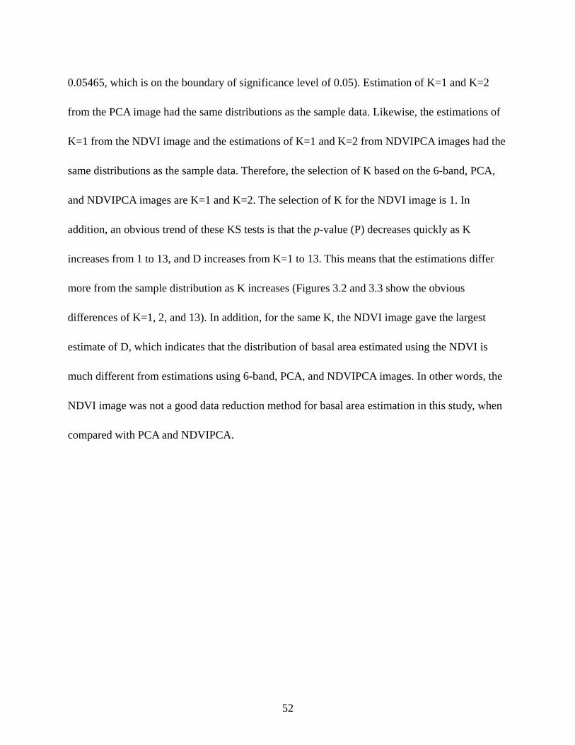
52
0.05465, which is on the boundary of significance level of 0.05). Estimation of K=1 and K=2
from the PCA image had the same distributions as the sample data. Likewise, the estimations of
K=1 from the NDVI image and the estimations of K=1 and K=2 from NDVIPCA images had the
same distributions as the sample data. Therefore, the selection of K based on the 6-band, PCA,
and NDVIPCA images are K=1 and K=2. The selection of K for the NDVI image is 1. In
addition, an obvious trend of these KS tests is that the p-value (P) decreases quickly as K
increases from 1 to 13, and D increases from K=1 to 13. This means that the estimations differ
more from the sample distribution as K increases (Figures 3.2 and 3.3 show the obvious
differences of K=1, 2, and 13). In addition, for the same K, the NDVI image gave the largest
estimate of D, which indicates that the distribution of basal area estimated using the NDVI is
much different from estimations using 6-band, PCA, and NDVIPCA images. In other words, the
NDVI image was not a good data reduction method for basal area estimation in this study, when
compared with PCA and NDVIPCA.
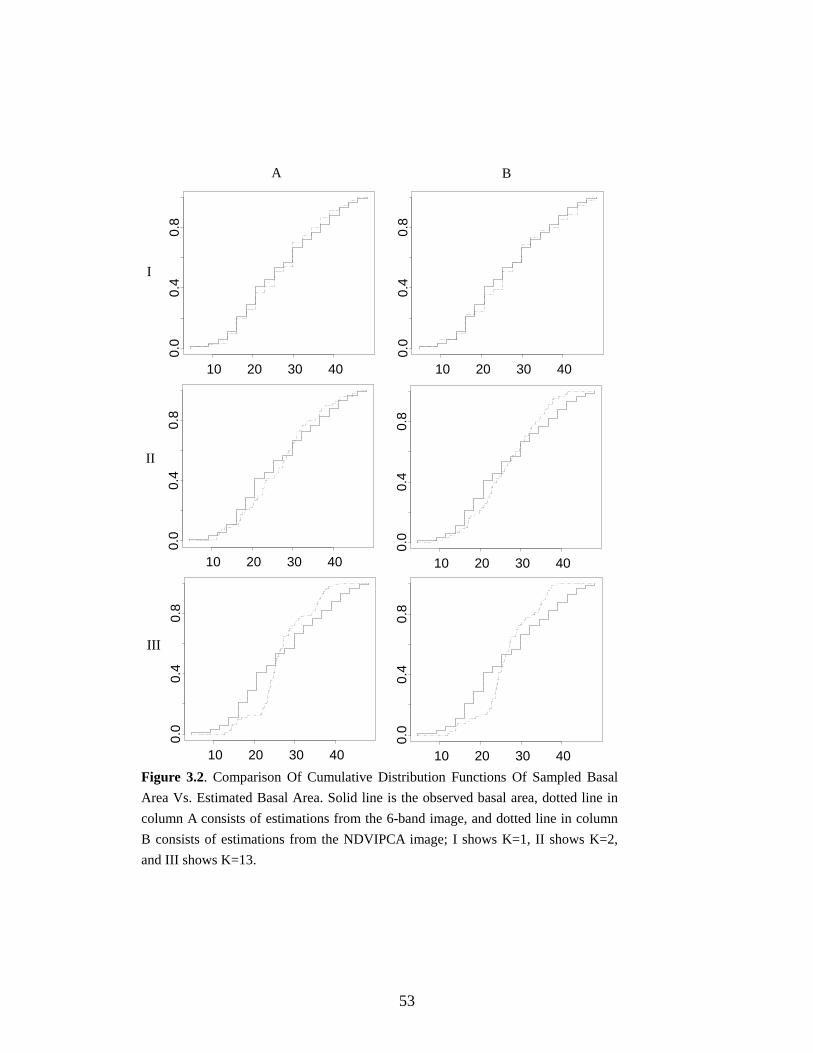
53
Figure 3.2. Comparison Of Cumulative Distribution Functions Of Sampled BasalArea Vs. Estimated Basal Area. Solid line is the observed basal area, dotted line incolumn A consists of estimations from the 6-band image, and dotted line in columnB consists of estimations from the NDVIPCA image; I shows K=1, II shows K=2,and III shows K=13.
10 20 30 40
0.0
0.4
0.8
10 20 30 40
0.0
0.4
0.8
10 20 30 40
0.0
0.4
0.8
10 20 30 40
0.0
0.4
0.8
10 20 30 40
0.0
0.4
0.8
10 20 30 40
0.0
0.4
0.8
A B
I
II
III
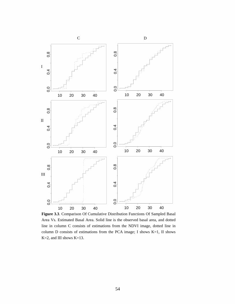
54
Figure 3.3. Comparison Of Cumulative Distribution Functions Of Sampled BasalArea Vs. Estimated Basal Area. Solid line is the observed basal area, and dottedline in column C consists of estimations from the NDVI image, dotted line incolumn D consists of estimations from the PCA image; I shows K=1, II showsK=2, and III shows K=13.
10 20 30 40
0.0
0.4
0.8
10 20 30 40
0.0
0.4
0.8
10 20 30 40
0.0
0.4
0.8
10 20 30 40
0.0
0.4
0.8
10 20 30 40
0.0
0.4
0.8
10 20 30 40
0.0
0.4
0.8
C D
I
II
III
55
The KS tests indicate significant differences between the distributions based on K=1 or K=2
and those estimations based on K>2. When K=1 or K=2, the distributions of the estimated data
have almost the same distributions as the sample data. However, the distributions of the
estimated data differ greatly from the sample data distribution when K > 2 (Table 3.6). As K
increases, the difference between the estimated and sample distributions also increases, although
the RMSE decreases. The estimated data from NDVI when K=13 shows the extreme situation, as
the vast majority of the data are compacted into a very narrow fraction of the plot (III, C in Fig.
3).
Based on the KS test results and the comparison of the CDF plots, we achieved very similar
estimations based on PCA, NDVIPCA, and 6-band images. The PCA image has two layers and
the NDVIPCA image has three layers, but the 6-band image has 6 layers. PCA and NDVIPCA
images save much more time in the computation process. PCA is a good method of data
reduction in image analysis. Therefore, we recommend remote sensing data reduction or
transformation and then conduct the KNN analysis using the transformed image for basal area
estimation.
3.7 Conclusions
This research focused on the problems of KNN methods, which are the selection of K values
and computation cost. The selection of K values was discussed comparing KS tests and CDF
plots. The PCA, NDVI, and the combination of PCA and NDVI images were used to save the
computation cost. K=1 or K=2 was the optimal selection according to the KS tests and CDF plots
56
in this research since estimations of basal area using K=1 and K=2 both have almost the same
distributions as the sample data.
We discussed and applied three methods of band reduction and transformation: PCA, NDVI,
and the combination of PCA and NDVI. Results indicate PCA was the optimal data reduction
method for this research because it produced similar basal area estimations to the 6-band and
NDVIPCA images. Since it has only two layers, much time is saved in distance computation.
The CDF plots show that the NDVI image is not a satisfactory method of data reduction for this
research. Although the estimation of K=1 has a similar distribution to the sample data, of the four
types of basal estimations using 6-band, PCA, NDVI, and NDVIPCA images, estimations based
on the NDVI image have the largest difference from sample data (Table 3.6, Figures 3.2 and 3.3),
when the estimations are compared to the sample data.
Overall, the comparison of KS tests and CDF plots is a relatively effective method of
selecting K when KNN is used for estimating, classifying, and mapping forest parameters. This
method seems more efficient than the available re-sampling statistics because the KS test is a
powerful test of whether the estimated and the sample data have the same or similar distributions.
The KS test and CDF plots also help us check the agreements of distributions between sample
and estimated data, which is useful for selecting an efficient data reduction approach. It is
difficult to determine which type of data reduction is better simply comparing SD and RMSE
using the available methods for selecting K values (Tables 3.1-5).
The critical point of K selection in forest inventory using KNN is whether the estimation has
the same or similar distribution as the sample. KNN is not only useful for global estimation, but
57
also for classification and spatial prediction in forest inventories. We believe that KNN can be
extensively applied in forest inventory and other related natural resource prediction and
classification. The characteristics of local vs. regional and place vs. space are also very important
in forest or natural resources management. Therefore, the estimations based on the selected K
should not only have smaller RMSE, but also similar distributions as the sample data.
It is difficult to select the optimal K based on direct calculation of RMSE and re-sampling
statistics because it seems that there are some trade-offs between choosing the smallest RMSE
and similar standard deviation (i.e., the similar distributions between the sample data and
estimated data). The KS test makes no assumptions on the distribution of data. The KS test and
CDF plots indicate the degree of differences in estimations for different Ks. As K increases, the
difference between the estimated distributions and the sample distribution also increases. A
suitable way to select K is the combination of KS test and CDF comparisons of the samples and
estimations. We advise using the KS test and CDF comparisons to select K values. Deciding on
the optimal K values, however, depends on the significance of the KS test and the CDF
comparisons between samples and estimations in the particular research. In this research, K=2
was the optimal choice, since its estimations have a similar distribution to the sample data and
smaller RMSE than that of K=1.
58
CHAPTER 4
GEOSTATISTICAL PREDICTION AND MAPPING
FOR LARGE AREA FOREST INVENTORY USING REMOTE SENSING DATA∗
4.1 Introduction
Large area forest inventory is important for understanding and managing forest resources
and ecosystems. The purpose of traditional large area forest inventory is to provide unbiased and
reliable forest resource information, though typically these inventories lack fine spatial resolution.
Remote sensing, the Global Positioning System (GPS), and geographic information systems
(GIS) provide new opportunities for forest inventory. By integrating remote sensing, GPS, and
GIS, it is possible to predict forest parameters at fine spatial resolutions. The research described
here develops a new systematic geostatistical approach for large area forest inventories, where
one type of forest parameter, such as basal area, height, health conditions, biomass, or carbon can
be incorporated as a response variable and the geostatistical approach can be used to predict
un-inventoried points. Using basal area as an illustration, this approach includes univariate
kriging (ordinary kriging and universal kriging) and multivariable kriging (cokriging and
regression kriging). The combination of bands 4, 3, and 2, as well as the combination of bands 5,
4, and 3, along with normalized difference vegetation index (NDVI) and principal components
∗ This research has been published online at www.ucgis.org/summer2006/studentpapers/Mengqm_July03_2006.pdf. It has been submitted to GIScience and Remote Sensing.
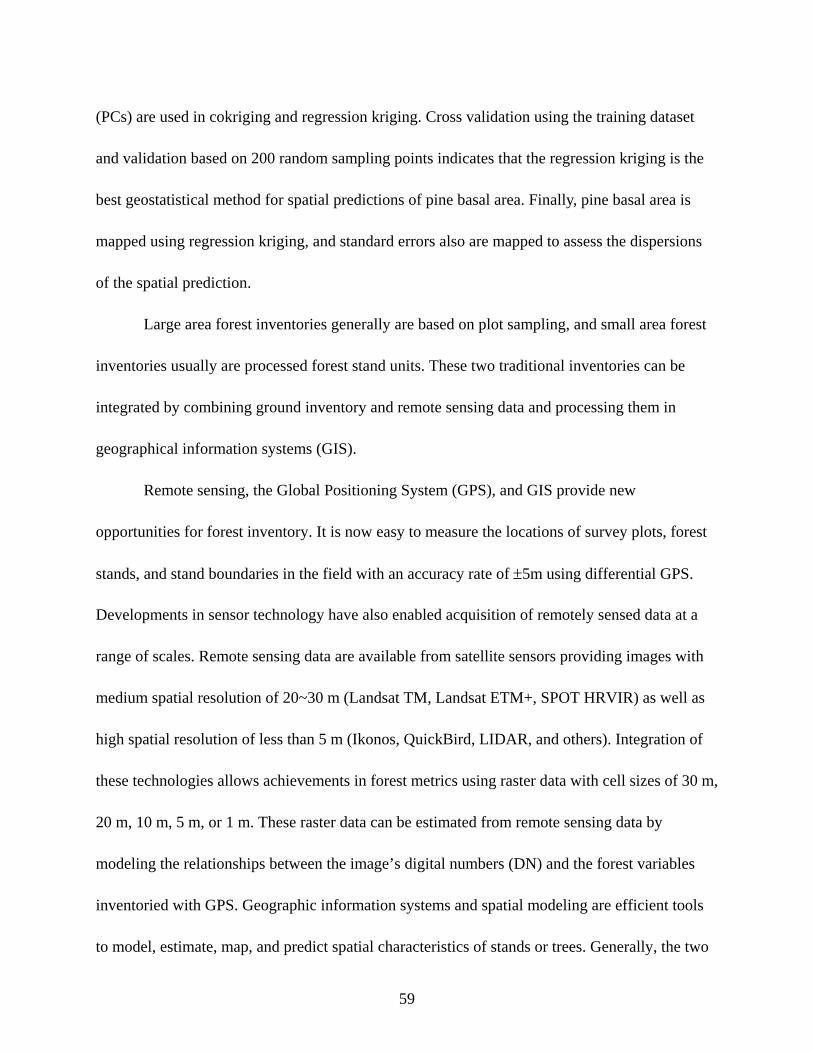
59
(PCs) are used in cokriging and regression kriging. Cross validation using the training dataset
and validation based on 200 random sampling points indicates that the regression kriging is the
best geostatistical method for spatial predictions of pine basal area. Finally, pine basal area is
mapped using regression kriging, and standard errors also are mapped to assess the dispersions
of the spatial prediction.
Large area forest inventories generally are based on plot sampling, and small area forest
inventories usually are processed forest stand units. These two traditional inventories can be
integrated by combining ground inventory and remote sensing data and processing them in
geographical information systems (GIS).
Remote sensing, the Global Positioning System (GPS), and GIS provide new
opportunities for forest inventory. It is now easy to measure the locations of survey plots, forest
stands, and stand boundaries in the field with an accuracy rate of ±5m using differential GPS.
Developments in sensor technology have also enabled acquisition of remotely sensed data at a
range of scales. Remote sensing data are available from satellite sensors providing images with
medium spatial resolution of 20~30 m (Landsat TM, Landsat ETM+, SPOT HRVIR) as well as
high spatial resolution of less than 5 m (Ikonos, QuickBird, LIDAR, and others). Integration of
these technologies allows achievements in forest metrics using raster data with cell sizes of 30 m,
20 m, 10 m, 5 m, or 1 m. These raster data can be estimated from remote sensing data by
modeling the relationships between the image’s digital numbers (DN) and the forest variables
inventoried with GPS. Geographic information systems and spatial modeling are efficient tools
to model, estimate, map, and predict spatial characteristics of stands or trees. Generally, the two
60
ways to obtain the fine spatial forest information are spatial modeling and nonspatial modeling.
Nonspatial modeling methods have been widely applied in forest research. Ordinary
least-squares (OLS) regressions are the common models applied for estimations of forest
variables (Ardö, 1992; Dungan, 1998; Trotter, Dymond & Goulding, 1997). K nearest neighbor
(KNN) methods for achieving forest metrics using remote sensing data have been applied in
Finland and America for forest inventories (Franco-Lopez, et al. 2001; Holmström and Fransson,
2003; Moeur and Stage, 1995; Tomppo, 1991). Artificial neural networks also are used for
estimating forest variables using remote sensing data (Foody & Boyd, 1999; Foody, 2000; Tatem
et al., 2001).
Tokola et al. (1996) applied both linear regression and the KNN method on forests in
the southern boreal vegetation zone in Finland using data from Landsat TM and SPOT. The
authors reported standard errors of stem volume prediction from 70 to 80 m3/ha (more than 60%
of the mean) at the plot level. Trotter et al. (1997) used Ordinary Least Squares to predict stem
volume of mature plantations in New Zealand and reported a root mean square error (RMSE)
greater than 100 m3/ha (with a mean stem volume of 413 m3/ha) for pixel predictions. The K
nearest neighbor method was applied by Holmström & Fransson (2003) to predict forest
variables using a combination of SPOT-4 and low-frequency radar data from the airborne
CARABAS system. The study by Holmström & Fransson (2003) used data from a coniferous
forest in southwest Sweden and reported RMSEs of 64% (of the mean) of stem volume using
optical data and 53% using the combination of optical and radar data. The stem volume of the
sample plots (10 m radius) was in the range of 0-750 m3/ha with a mean value of 171 m3/ha.
61
Many studies have conducted spatial predictions using remotely sensed data (Atkinson et
al. 1994; Atkinson and Lewis, 2000; Chica-Olmo and Abarca-Hernandez, 2000; Curran, 1988;
Curran and Atkinson 1998; Dungan 1998; Dungan, et al.1994; Lark, 1996). Few studies have
been conducted on estimations of forestry relevant variables using spatial models, though, a large
number of spatial-statistical and prediction models are available in the literature (e.g. Cressie,
1993; Goovaerts, 1997; Odeh, et al. 1995; Odeh and McBratney, 2000; Wackernagel, 1994).
Berterretche et al. (2005), Tuominen et al.(2003), and Zhang et al (2004) applied geostatistical
models to estimate forest variables, leaf area index, and classify forest lands based on remote
sensing data. Gilbert & Lowell (1997) used kriging to predict stem volume in a 1500 ha balsam
fir (Abies balsamea) dominated forest. Prediction based on 5.6 m and 11.3 m radius plots
resulted in a prediction RMSE of 54% (of the mean) and 39-46%, respectively. Similar accuracy
was obtained by prediction using the sample average only. Methodologically, the accuracy rate
of the predicted variable could be improved by incorporating close field observations as
predictors in spatial modeling.
Rarely has research explored the integration of remote sensing data, GPS, ground data,
GIS, and geostatistics to estimate forest parameters at a fine spatial resolution for large areas.
One systematic geostatistical approach for spatial forest inventory is developed and explored in
this research. Compared to the typical ordinary kriging (OK) and universal kriging (UK) using
only one variable, this research develops a systematic geostatistical approach—co-kriging (CoK)
and regression kriging (RK) using remotely sensed data as predictors—to improve spatial
predictions of forest variables by integrating GPS, ground inventory data, remote sensing, and
62
GIS. This systematic geostatistical approach is summarized in a flow chart (Figure 4.1), and
provides new insights for forest parameter estimation, and not only considers the associations
between one forest parameter and DN but also incorporates the spatial dependence of the forest
parameter into the process of spatial prediction. In this study, basal area is used as the response
variable to conduct this geostatistical approach.
In addition to analyzing spatial characteristics of an integrated GIS with ground and
remote sensing data, it is also necessary to analyze nonspatial data; for example, the selection of
Ground Data Forest parameter + GPS data Basal area/Dominant heights/Age Healthy conditions Biomass/Carbon Others
GIS Data Integration
Remote Sensing Data Georegistration Radiometric correction Spectral enhancement Others
Non-spatial Analysis
Variograms Cross Variograms
Ordinary Kriging Universal Kriging
Co-Kriging Regression Kriging
Trend?
Kriging Evaluation—Cross Validation and Validation Based on Random Samples
Selection of Kriging Mehods and Geostatistical Mapping of Forest Parameters
Figure 4.1 A Systematic Geostatistical Approach For Predicting Forest Parameters Using Remotely SensedData.
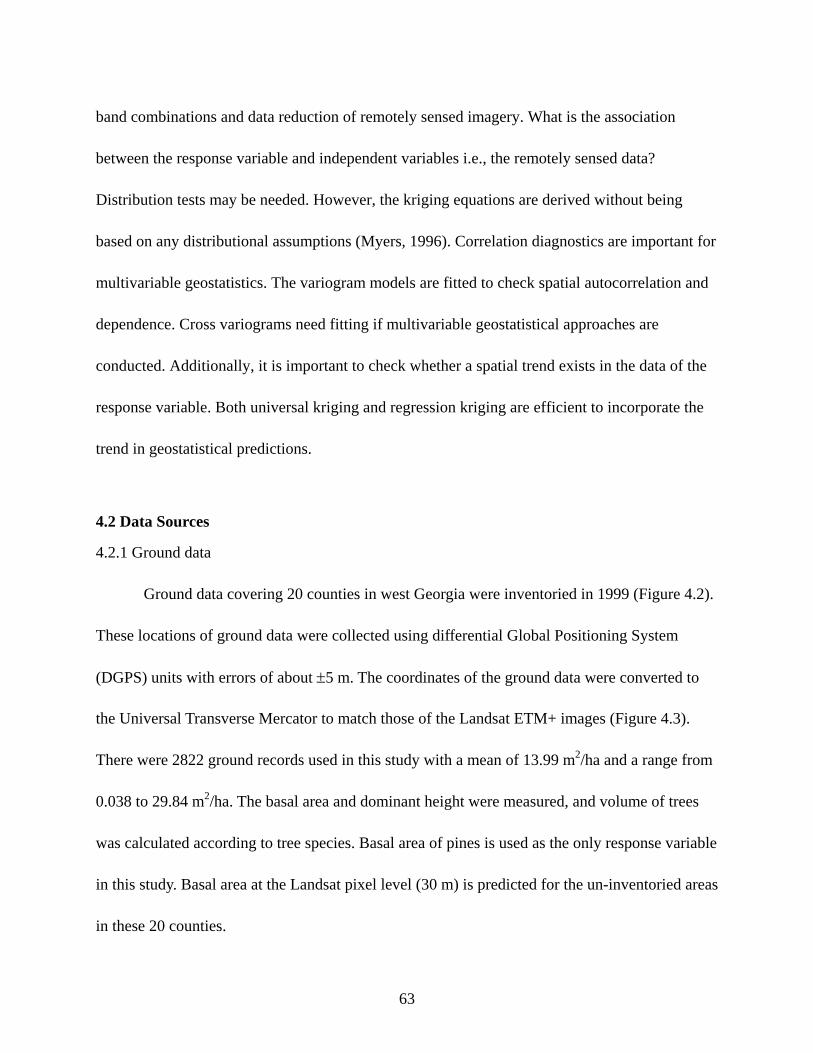
63
band combinations and data reduction of remotely sensed imagery. What is the association
between the response variable and independent variables i.e., the remotely sensed data?
Distribution tests may be needed. However, the kriging equations are derived without being
based on any distributional assumptions (Myers, 1996). Correlation diagnostics are important for
multivariable geostatistics. The variogram models are fitted to check spatial autocorrelation and
dependence. Cross variograms need fitting if multivariable geostatistical approaches are
conducted. Additionally, it is important to check whether a spatial trend exists in the data of the
response variable. Both universal kriging and regression kriging are efficient to incorporate the
trend in geostatistical predictions.
4.2 Data Sources
4.2.1 Ground data
Ground data covering 20 counties in west Georgia were inventoried in 1999 (Figure 4.2).
These locations of ground data were collected using differential Global Positioning System
(DGPS) units with errors of about ±5 m. The coordinates of the ground data were converted to
the Universal Transverse Mercator to match those of the Landsat ETM+ images (Figure 4.3).
There were 2822 ground records used in this study with a mean of 13.99 m2/ha and a range from
0.038 to 29.84 m2/ha. The basal area and dominant height were measured, and volume of trees
was calculated according to tree species. Basal area of pines is used as the only response variable
in this study. Basal area at the Landsat pixel level (30 m) is predicted for the un-inventoried areas
in these 20 counties.
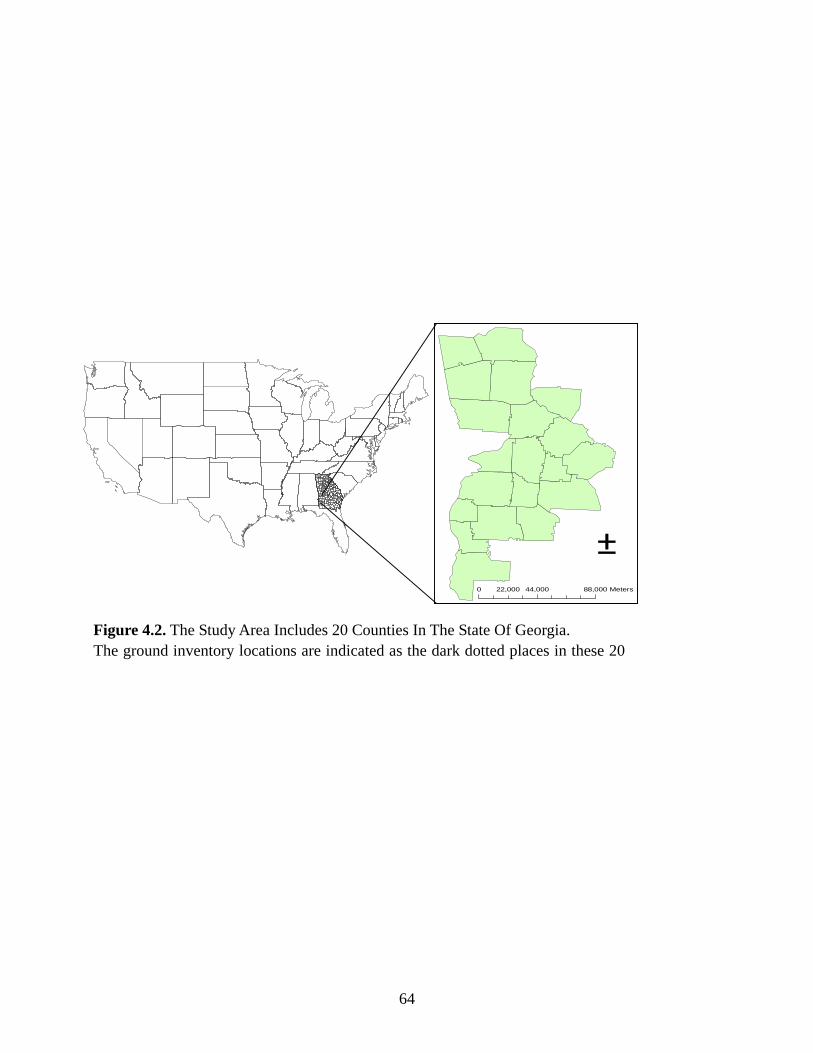
64
±0 44,000 88,00022,000 Meters
Figure 4.2. The Study Area Includes 20 Counties In The State Of Georgia. The ground inventory locations are indicated as the dark dotted places in these 20
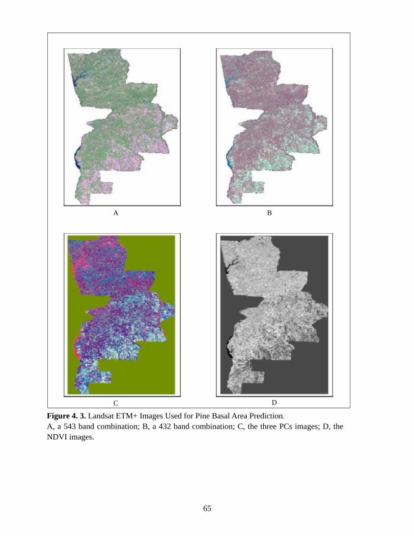
65
A B
C D
Figure 4. 3. Landsat ETM+ Images Used for Pine Basal Area Prediction. A, a 543 band combination; B, a 432 band combination; C, the three PCs images; D, the NDVI images.
66
4.2.2 Remote sensing data
Landsat 7 Enhanced Thematic Mapper Plus (ETM+) images (Path/Row: 19/37 and 19/38)
acquired on 10 September 1999 from the USGS Earth Resource Observation System Data Center
were used in this research. Atmospheric conditions were clear at the time of image acquisition,
and the data had been corrected for the radiometric and geometric distortions of the images to the
standard Level 1G before delivery. Two Landsat images covering this study area were masked
after the geometric corrections using U.S. Geological Survey (USGS) digital orthophoto
quarterquads (DOQQs) as the sources of control (RMSE is less than 10 m). This resulted in a
4449 pixel by 9010 row 6-band (i.e., 1, 2, 3, 4, 5, and 7) image for analysis.
Band Combinations
Band 1 of Landsat images contributes little for vegetation analysis. Studies indicate that
as the leaf coverage changes from 0% to 11.9%, 43.2%, and 87.6%, very little change occurs in
the reflectance of band 1 (0.4-0.5 um) (Short, 1999). The differences of reflectance increase from
0.5 to 0.8 um as leaves change. The differences of reflectance in the mid-infrared ranges are very
close to the differences in the near infrared ranges. Band 7 of Landsat images is not used as an
independent variable. Bands 2, 3, 4 and 5 are used, and 432 and 543 band combinations are
applied to estimate pine basal area.
Principal Component Analysis
Principal component analysis (PCA) is the most frequently used technique for remote
sensing data reduction. Generally, remotely sensed data, such as Landsat images, are highly
correlated among the adjacent spectral bands (Barnsley, 1999). The Landsat bands are
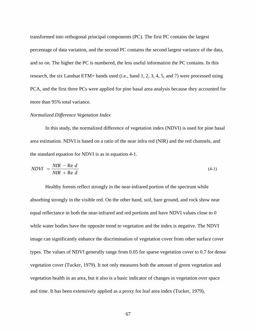
67
transformed into orthogonal principal components (PC). The first PC contains the largest
percentage of data variation, and the second PC contains the second largest variance of the data,
and so on. The higher the PC is numbered, the less useful information the PC contains. In this
research, the six Landsat ETM+ bands used (i.e., band 1, 2, 3, 4, 5, and 7) were processed using
PCA, and the first three PCs were applied for pine basal area analysis because they accounted for
more than 95% total variance.
Normalized Difference Vegetation Index
In this study, the normalized difference of vegetation index (NDVI) is used for pine basal
area estimation. NDVI is based on a ratio of the near infra red (NIR) and the red channels, and
the standard equation for NDVI is as in equation 4-1.
Healthy forests reflect strongly in the near-infrared portion of the spectrum while
absorbing strongly in the visible red. On the other hand, soil, bare ground, and rock show near
equal reflectance in both the near-infrared and red portions and have NDVI values close to 0
while water bodies have the opposite trend to vegetation and the index is negative. The NDVI
image can significantly enhance the discrimination of vegetation cover from other surface cover
types. The values of NDVI generally range from 0.05 for sparse vegetation cover to 0.7 for dense
vegetation cover (Tucker, 1979). It not only measures both the amount of green vegetation and
vegetation health in an area, but it also is a basic indicator of changes in vegetation over space
and time. It has been extensively applied as a proxy for leaf area index (Tucker, 1979),
dNIRdNIRNDVI
ReRe
+−
= (4-1)
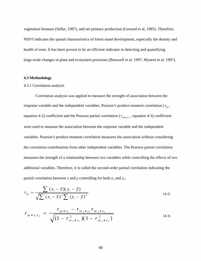
68
vegetation biomass (Seller, 1987), and net primary production (Goward et al, 1985). Therefore,
NDVI indicates the spatial characteristics of forest stand development, especially the density and
health of trees. It has been proven to be an efficient indicator in detecting and quantifying
large-scale changes in plant and ecosystem processes (Braswell et al. 1997; Myneni et al. 1997).
4.3 Methodology
4.3.1 Correlation analysis
Correlation analysis was applied to measure the strength of association between the
response variable and the independent variables. Pearson’s product-moment correlation ( xyr ,
equation 4-2) coefficient and the Pearson partial correlation (21zzxyr • , equation 4-3) coefficient
were used to measure the association between the response variable and the independent
variables. Pearson’s product-moment correlation measures the association without considering
the correlation contributions from other independent variables. The Pearson partial correlation
measures the strength of a relationship between two variables while controlling the effects of two
additional variables. Therefore, it is called the second-order partial correlation indicating the
partial correlation between x and y controlling for both z1 and z2.
(4-2) ∑ ∑∑
−−
−−=
22 )()(
))((
yyxx
yyxxr
ii
iixy
(4-3) )1)(1( 221212
12121
21
zyzzxz
zyzzxzzxyzzxy
rr
rrrr
••
••••
−−
−=
69
4.3.2 Geostatistical approach
Geostatistical methods are based on the theory of regionalized variables (Matheron,
1965), which makes the assumption that data are observations of stochastic variables. We can
consider a spatial variable as a realization of a random function represented by a stochastic
model.
One of the key steps in geostatistical modeling is the semivariogram, a function
describing the spatial dependence of the spatial variable. The semivariogram has been used
widely in remote sensing to determine spatial structures (Curran, 1988; Warren, et al., 1990;
Atkinson & Lewis, 2000). Based on the semivariogram, the geostatistical process derives
optimal linear unbiased spatial prediction methods (i.e., kriging) by minimizing mean-squared
prediction error. However, the assumptions of stationarity, which often are not met by the
field-sampled data sets, and the requirement of a large dataset to define the spatial
autocorrelation, result in the limitations of univariate kriging. Fortunately, geostatistical methods
also provide optimal prediction methods using auxiliary data. Large volumes of auxiliary data for
forest research are available now, such as remote sensing data. Incorporating the auxiliary data,
co-kriging and regression kriging, as described below, can increase prediction accuracy. The
gstat package (Pebesma, 2005) is mainly referenced for variogram and kriging methods as
follows.
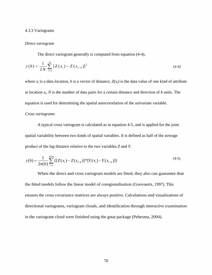
70
4.3.3 Variograms
Direct variogram
The direct variogram generally is computed from equation (4-4),
where xi is a data location, h is a vector of distance, Z(xi) is the data value of one kind of attribute
at location xi, N is the number of data pairs for a certain distance and direction of h units. The
equation is used for determining the spatial autocorrelation of the univariate variable.
Cross variograms
A typical cross variogram is calculated as in equation 4-5, and is applied for the joint
spatial variability between two kinds of spatial variables. It is defined as half of the average
product of the lag distance relative to the two variables Z and Y.
When the direct and cross variogram models are fitted, they also can guarantee that
the fitted models follow the linear model of coregionalisation (Goovaerts, 1997). This
ensures the cross covariance matrices are always positive. Calculations and visualizations of
directional variograms, variogram clouds, and identification through interactive examination
in the variogram cloud were finished using the gstat package (Pebesma, 2004).
∑=
+−=N
ihii xZxZ
Nh
1
2)]()([21)(γ (4-4)
∑=
++ −−=)(
1
)]}()([*)]()({[)(2
1)(hn
ihiihii xYxYxZxZ
hnhγ (4-5)
71
4.3.4 Kriging
Ordinary kriging and universal kriging
Ordinary kriging (OK) is identical to multiple linear regression with a couple of
important differences. The ordinary kriging model is as in equation 4-6. Z(s0) is the value to be
interpolated at location s0, )( isz are the sampled values at their locations, and iλ are the weights
to be assigned to each sampled value. Universal kriging is applied when a trend exists. Universal
kriging is often fitted using a polynomial equation, which is similar to the equation 4-6 to
analyze the trend across the study area.
Cokriging
For forest applications, a few studies using remote sensing data have been conducted
using the geostatistical approach. Dungan et al. (1994) and Dungan (1998) applied co-kriging
and a stochastic simulation method for forest management using synthetic remote sensing
datasets.
Co-kriging (CoK) is an extension of kriging, and is a method for estimating one or more
variables of interest using data from several variables by incorporating not only spatial
correlation but also inter-variable correlation. Co-kriging is a very versatile and rigorous
statistical technique for spatial point estimation when both primary and auxiliary attributes are
available. It is defined as in equation 4-7. If each component of z(s0) satisfies the intrinsic
hypothesis (Journel and Huijbregts, 1978), then equation 4-5 is unbiased if
∑−
=n
iii szsZ
10 )()( λ (4-6)
72
where I is an identity matrix = [1,0,…,0]T and T indicates a transpose, and •Λ j are the weights
associated with prediction. Equation 4-7 is
where z(sj) is the vector z1(sj)…zm(sj). ),( ji ssΓ and ),( 0ssiΓ are the cross variograms, and
Ψ is the Lagrange Multiplier for i from 1 to n.
According to the sample relations between the primary variable and the auxiliary
variables, CoK could be described in several ways as follows. The most efficient way to predict
the primary variable is to use the auxiliary variables to cokrig it into dense grid locations. This is
named heterotopic cokriging (Wackernagel, 1994). Isotopic cokriging requires that data on both
the target variable and co-variables be measured at all sample locations. A variant of both is
generalized cokriging (Myers, 1982) that involves simultaneous prediction of all the correlated
variables into more dense locations. The complete case is the case where the covariates and the
primary variable do not share any common locations. A more general type applied using remote
sensing data is collocated cokriging, where covariates are available at all interpolation locations,
although the primary variable is available at only a few locations. When CoK is compared to
univariate kriging, no new concept is added, but there is heavier notation associated with having
several variables (Goovaerts, 1997).
∑=
•Λ=n
jjjszsZ
10 )()( (4-7)
∑=
• Ι=Λn
jj
1
(4-8)
nissss i
v
ji ,...,1),(),( 01
=Γ=Ψ+Γ∑=φ
(4-9)
73
Regression kriging
Regession kriging (RK) is a hybrid method that combines either a simple or
multiple-linear regression model (or a variant of the generalized linear model (GLM) and
regression trees) with kriging (Odeh et al., 1995; Goovaerts, 1997). In the process of RK, kriging
with uncertainty introduces the regression residuals (i.e., the model uncertainty) into the kriging
system, which is then applied directly to predict the primary variable. The predictions are
combined from two parts; one is the estimation obtained by regressing the primary variable on
the auxiliary variables; the second part is the residual estimated from the ordinary kriging.
Regression kriging is estimated as follows:
where kβ are trend model coefficients, optimally estimated using generalized least squares;
iω are weights determined by the semivariance function, and l are the regression residuals. In
the gstat package, univarite kriging and multivariable kriging are applied for pine basal area
prediction (Pebesma, 2004, 2005).
4.4 Model Evaluation
In this study, different geostatistical models are developed and applied for pine basal area
prediction. There are always discrepancies between true and predicted values. It is necessary to
validate the models and check which is more efficient. For this geostatistical approach, two
methods for assessing models are applied. One method is cross validation, which is used to
)(ˆ)(ˆ)(ˆ000 ssmsZrk l+= (4-10)
(4-11) nisqsssqsZ i
n
ii
v
kkkrk ,...,1,1)()(*)()(*ˆ)(ˆ
001
000
0 ==+= ∑∑==
lωβ
74
validate whether the model fits the training data. The second method is validation based on
random samples outside of the training data set. We developed 200 random points to check
which model is more efficient in spatial predictions of pine basal area.
There are many different measures for checking discrepancies and each has its
advantages and weaknesses. Details about forecast evaluation were discussed by Murphy and
Katz (1985). Typically, four criteria, standard deviation (SD), bias error (BE), root mean square
error (RMSE), and mean-absolute error (MAE) are used to directly compare forecast and
observation. Standard deviation is the measure of dispersion from the mean of a particular
parameter as illustrated by equation 4-12.
where N is the size of the sample, Xn is the sample values and X is the mean of the sample. The
bigger the SD, the larger the dispersion of the estimations is from the mean. For the error term,
SD typically is used to measure the extent that forecast error differs from the mean. In this study,
the SD of errors (SDe) is computed to analyze dispersions of errors across the whole study area.
Bias error is used to measure whether the model under-forecasts or over-forecasts a
parameter and is defined in the equation:
where N is the total number of comparisons, fX is the forecast value, and oX is the observed
value. A positive BE indicates a tendency to overpredict while a negative BE implies under
predictions.
2/1
1
2)(1
1
−
−= ∑
=
N
nn XX
NSD (4-12)
)(1)(1
o
N
nf XX
NXBE −= ∑
=(4-13)
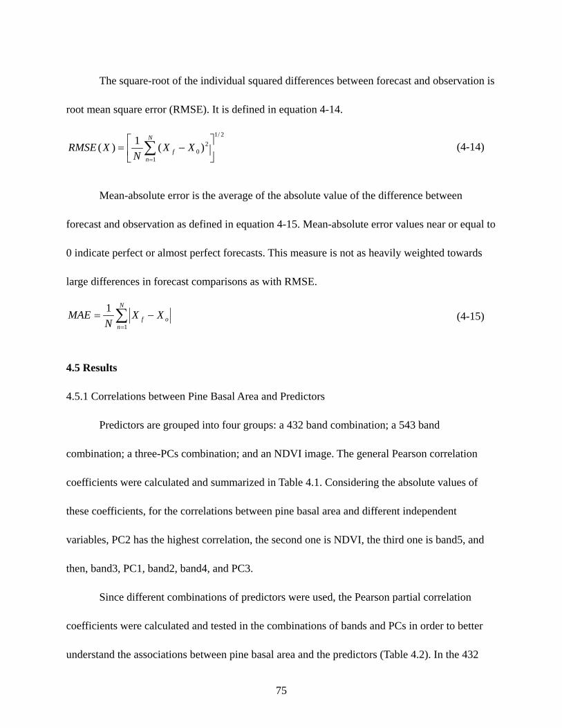
75
The square-root of the individual squared differences between forecast and observation is
root mean square error (RMSE). It is defined in equation 4-14.
Mean-absolute error is the average of the absolute value of the difference between
forecast and observation as defined in equation 4-15. Mean-absolute error values near or equal to
0 indicate perfect or almost perfect forecasts. This measure is not as heavily weighted towards
large differences in forecast comparisons as with RMSE.
4.5 Results
4.5.1 Correlations between Pine Basal Area and Predictors
Predictors are grouped into four groups: a 432 band combination; a 543 band
combination; a three-PCs combination; and an NDVI image. The general Pearson correlation
coefficients were calculated and summarized in Table 4.1. Considering the absolute values of
these coefficients, for the correlations between pine basal area and different independent
variables, PC2 has the highest correlation, the second one is NDVI, the third one is band5, and
then, band3, PC1, band2, band4, and PC3.
Since different combinations of predictors were used, the Pearson partial correlation
coefficients were calculated and tested in the combinations of bands and PCs in order to better
understand the associations between pine basal area and the predictors (Table 4.2). In the 432
2/1
1
20 )(1)(
−= ∑
=
N
nf XX
NXRMSE (4-14)
∑=
−=N
nof XX
NMAE
1
1(4-15)
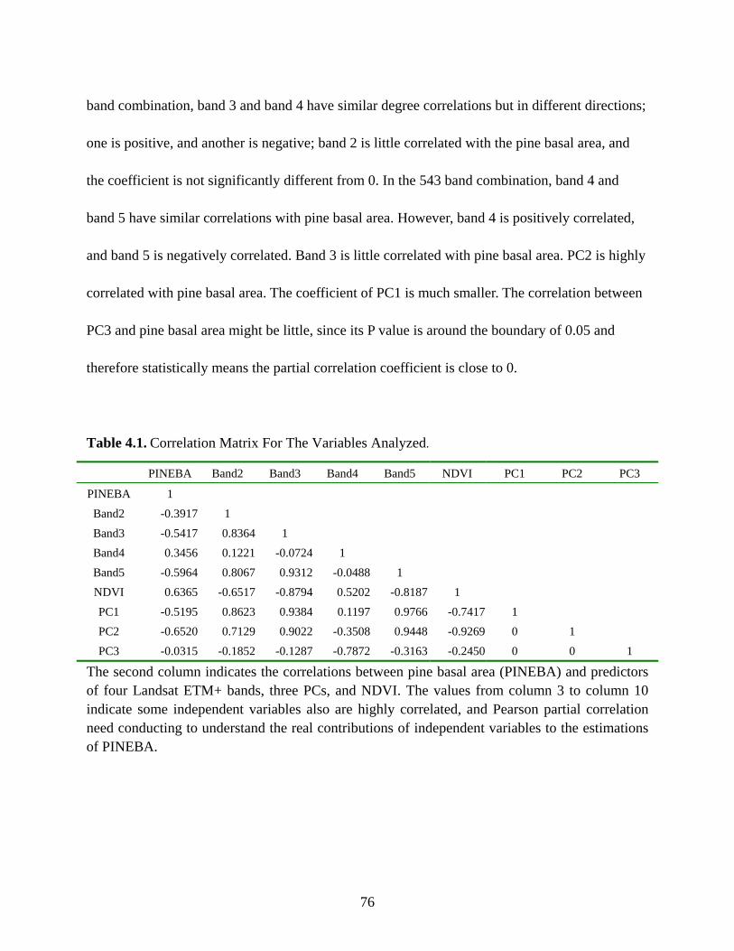
76
band combination, band 3 and band 4 have similar degree correlations but in different directions;
one is positive, and another is negative; band 2 is little correlated with the pine basal area, and
the coefficient is not significantly different from 0. In the 543 band combination, band 4 and
band 5 have similar correlations with pine basal area. However, band 4 is positively correlated,
and band 5 is negatively correlated. Band 3 is little correlated with pine basal area. PC2 is highly
correlated with pine basal area. The coefficient of PC1 is much smaller. The correlation between
PC3 and pine basal area might be little, since its P value is around the boundary of 0.05 and
therefore statistically means the partial correlation coefficient is close to 0.
Table 4.1. Correlation Matrix For The Variables Analyzed.
PINEBA Band2 Band3 Band4 Band5 NDVI PC1 PC2 PC3
PINEBA 1 Band2 -0.3917 1 Band3 -0.5417 0.8364 1 Band4 0.3456 0.1221 -0.0724 1 Band5 -0.5964 0.8067 0.9312 -0.0488 1 NDVI 0.6365 -0.6517 -0.8794 0.5202 -0.8187 1 PC1 -0.5195 0.8623 0.9384 0.1197 0.9766 -0.7417 1 PC2 -0.6520 0.7129 0.9022 -0.3508 0.9448 -0.9269 0 1 PC3 -0.0315 -0.1852 -0.1287 -0.7872 -0.3163 -0.2450 0 0 1
The second column indicates the correlations between pine basal area (PINEBA) and predictors of four Landsat ETM+ bands, three PCs, and NDVI. The values from column 3 to column 10 indicate some independent variables also are highly correlated, and Pearson partial correlation need conducting to understand the real contributions of independent variables to the estimations of PINEBA.

77
Table 4.2. Partial Correlations Analysis.
234 band combination 345 band combination Band2 Band3 Band4 Band3 Band4 Band5
rxy 0.0129 -0.3350 0.3436 0.0828 0.3997 -0.3429 P value 0.4976 <.0001 <.0001 <.0001 <.0001 <.0001
Pearson partial correlation coefficients (r) were calculated by eliminating effects due to the correlations between pine basal area and the other two variables in the band combinations. For example, the correlation between pine basal area and band2 is 0.0129 when the contributions from band3 and band4 were removed. This correlation is not significantly different from 0, since the P value is 0.4976 which is much bigger than 0.05.
4.5.2 Variograms and Spatial Dependence
Variograms were used to spatially analyze the surface properties of pine basal area. Based
on the variogram cloud, the empirical semivariogram model was created. The different types of
semivariogram models used to fit the points include exponential, Gaussian, circular, spherical,
tetraspherical, pentaspherical, Hole effect, K-Bessel, and J-Bessel models. The spherical model
had the best fits and was selected as the theoretical model applied for spatial predictions. The fit
of the spherical model has a nugget of 5, a partial sill of 450, and a range of 750. Also, there was
no obvious trend existing among the pine basal area across the study area.
The characteristics of the semivariogram also may be affected by the directions, which
result from a special geographic phenomenon. For example, a certain kind of species exists and
crosses the area in a certain direction. It is therefore necessary to check anisotropy.
Semivariogram analyses at directions 0, 45, 90, 135, 180, 225, 270, and 315 were conducted and
indicated similar spatial dependence at these eight directions (Figure 4.4). It is not necessary to
analyze anisotropic effects in spatial predictions.
78
4.5.3 Assessment of Pine Basal Area Estimation
We first applied Univariate kriging (i.e., OK and UK) to estimate the pine basal area
using 2822 ground inventory points. The UK was used to check whether it is effective compared
to the OK, though there was no obvious trend of pine basal area existing across the study area.
Four types of co-kriging were applied using the 432 band combination, the 543 band
combination, NDVI, and PCs as the auxiliary data. At last, four groups of regression kriging
were conducted using the 432 band combination, the 543 band combination, NDVI, and PCs as
predictors.
Figure 4.4 Semivariogram Modeling Effects of Eight Different Directions
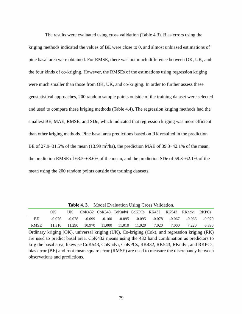
79
The results were evaluated using cross validation (Table 4.3). Bias errors using the
kriging methods indicated the values of BE were close to 0, and almost unbiased estimations of
pine basal area were obtained. For RMSE, there was not much difference between OK, UK, and
the four kinds of co-kriging. However, the RMSEs of the estimations using regression kriging
were much smaller than those from OK, UK, and co-kriging. In order to further assess these
geostatistical approaches, 200 random sample points outside of the training dataset were selected
and used to compare these kriging methods (Table 4.4). The regression kriging methods had the
smallest BE, MAE, RMSE, and SDe, which indicated that regression kriging was more efficient
than other kriging methods. Pine basal area predictions based on RK resulted in the prediction
BE of 27.9~31.5% of the mean (13.99 m2/ha), the prediction MAE of 39.3~42.1% of the mean,
the prediction RMSE of 63.5~68.6% of the mean, and the prediction SDe of 59.3~62.1% of the
mean using the 200 random points outside the training datasets.
Table 4. 3. Model Evaluation Using Cross Validation. OK UK CoK432 CoK543 CoKndvi CoKPCs RK432 RK543 RKndvi RKPCs
BE -0.076 -0.078 -0.099 -0.100 -0.095 -0.095 -0.078 -0.067 -0.066 -0.070RMSE 11.310 11.290 10.970 11.000 11.010 11.020 7.020 7.000 7.220 6.890
Ordinary kriging (OK), universal kriging (UK), Co-kriging (Cok), and regression kriging (RK) are used to predict basal area. CoK432 means using the 432 band combination as predictors to krig the basal area, likewise CoK543, CoKndvi, CoKPCs, RK432, RK543, RKndvi, and RKPCs; bias error (BE) and root mean square error (RMSE) are used to measure the discrepancy between observations and predictions.
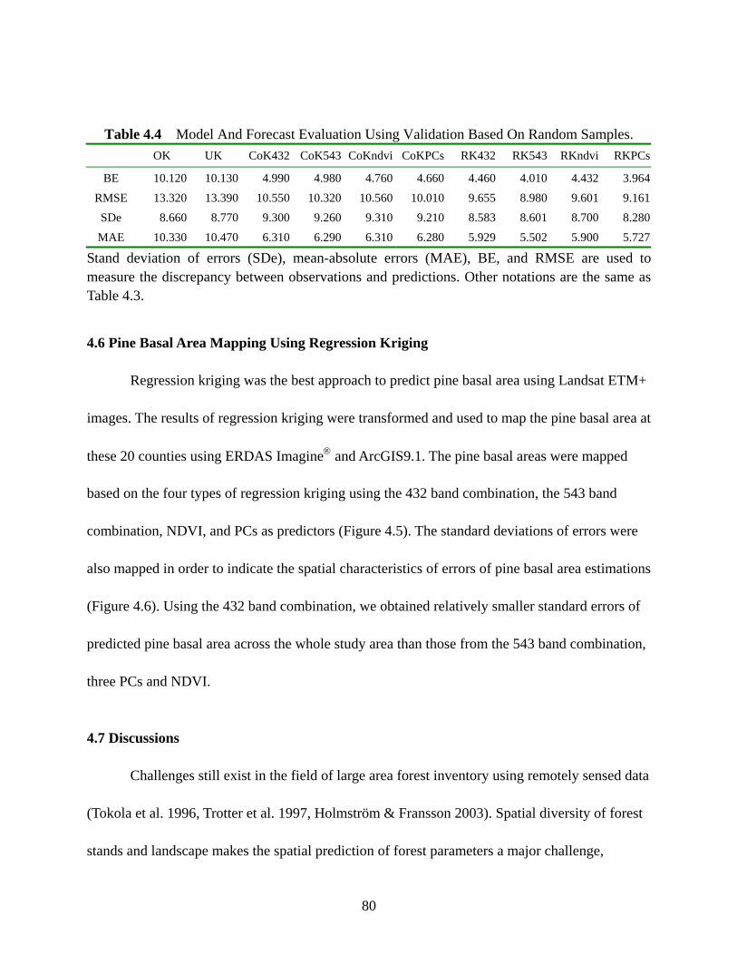
80
Table 4.4 Model And Forecast Evaluation Using Validation Based On Random Samples. OK UK CoK432 CoK543 CoKndvi CoKPCs RK432 RK543 RKndvi RKPCs
BE 10.120 10.130 4.990 4.980 4.760 4.660 4.460 4.010 4.432 3.964RMSE 13.320 13.390 10.550 10.320 10.560 10.010 9.655 8.980 9.601 9.161SDe 8.660 8.770 9.300 9.260 9.310 9.210 8.583 8.601 8.700 8.280MAE 10.330 10.470 6.310 6.290 6.310 6.280 5.929 5.502 5.900 5.727
Stand deviation of errors (SDe), mean-absolute errors (MAE), BE, and RMSE are used to measure the discrepancy between observations and predictions. Other notations are the same as Table 4.3.
4.6 Pine Basal Area Mapping Using Regression Kriging
Regression kriging was the best approach to predict pine basal area using Landsat ETM+
images. The results of regression kriging were transformed and used to map the pine basal area at
these 20 counties using ERDAS Imagine and ArcGIS9.1. The pine basal areas were mapped
based on the four types of regression kriging using the 432 band combination, the 543 band
combination, NDVI, and PCs as predictors (Figure 4.5). The standard deviations of errors were
also mapped in order to indicate the spatial characteristics of errors of pine basal area estimations
(Figure 4.6). Using the 432 band combination, we obtained relatively smaller standard errors of
predicted pine basal area across the whole study area than those from the 543 band combination,
three PCs and NDVI.
4.7 Discussions
Challenges still exist in the field of large area forest inventory using remotely sensed data
(Tokola et al. 1996, Trotter et al. 1997, Holmström & Fransson 2003). Spatial diversity of forest
stands and landscape makes the spatial prediction of forest parameters a major challenge,
81
although the remote sensing data are highly associated with forest features. For example, forest
stands may have very similar values of biomass/carbon but have different spectral characteristics
because of differences in species. The differences of spectral characteristics between plantations
and natural stands might exist although the stands have many of the same characteristics, such as
same species, same age, and same density. These differences will add noise when the prediction
models are fitted based on the associations between remotely sensed data and ground-inventoried
data.
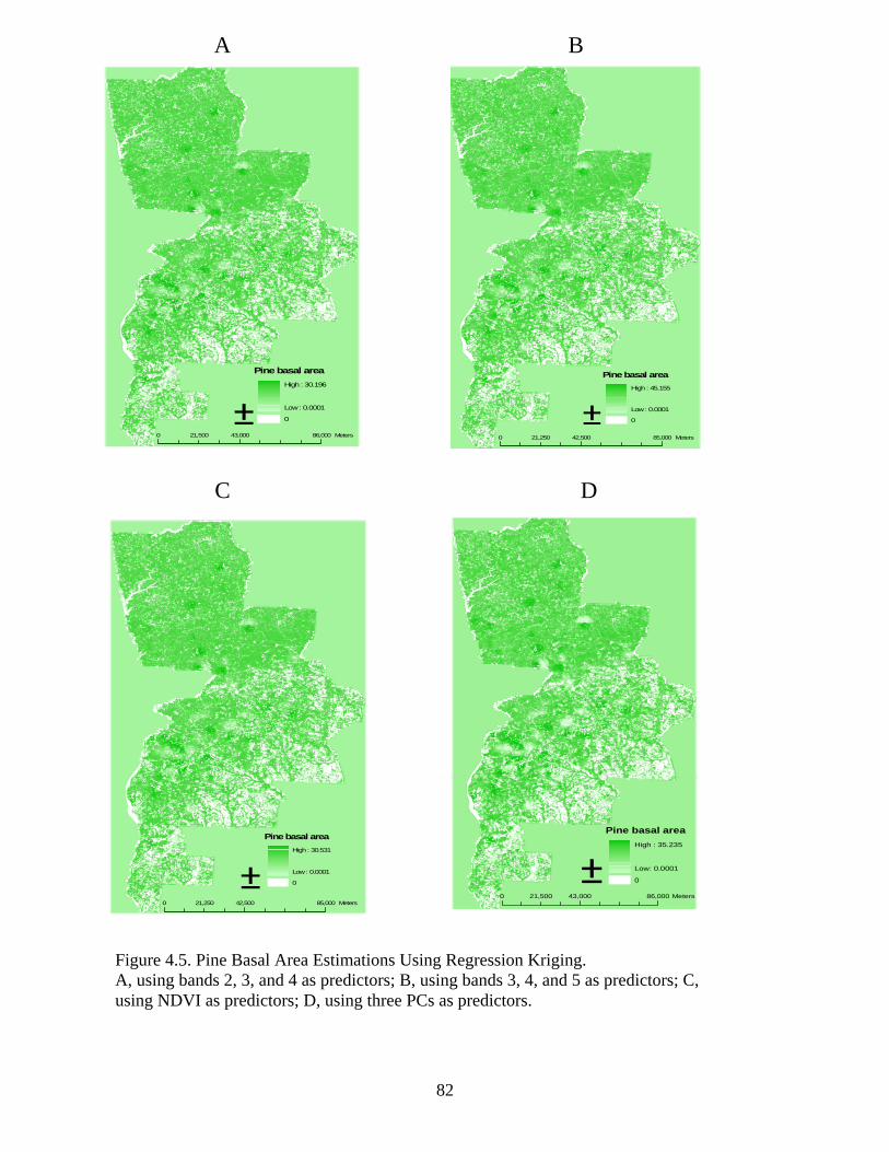
82
±
Pine basal areaHigh : 45.155
Low : 0.0001
0
0 42,500 85,00021,250 Meters
Pine basal areaHigh : 30.196
Low : 0.0001
0±0 43,000 86,00021,500 Meters
A B
Pine basal areaHigh : 30.531
Low : 0.0001
0±0 42,500 85,00021,250 Meters
C
±0 43,000 86,00021,500 Meters
Pine basal areaHigh : 35.235
Low: 0.0001
0
D
Figure 4.5. Pine Basal Area Estimations Using Regression Kriging. A, using bands 2, 3, and 4 as predictors; B, using bands 3, 4, and 5 as predictors; C, using NDVI as predictors; D, using three PCs as predictors.
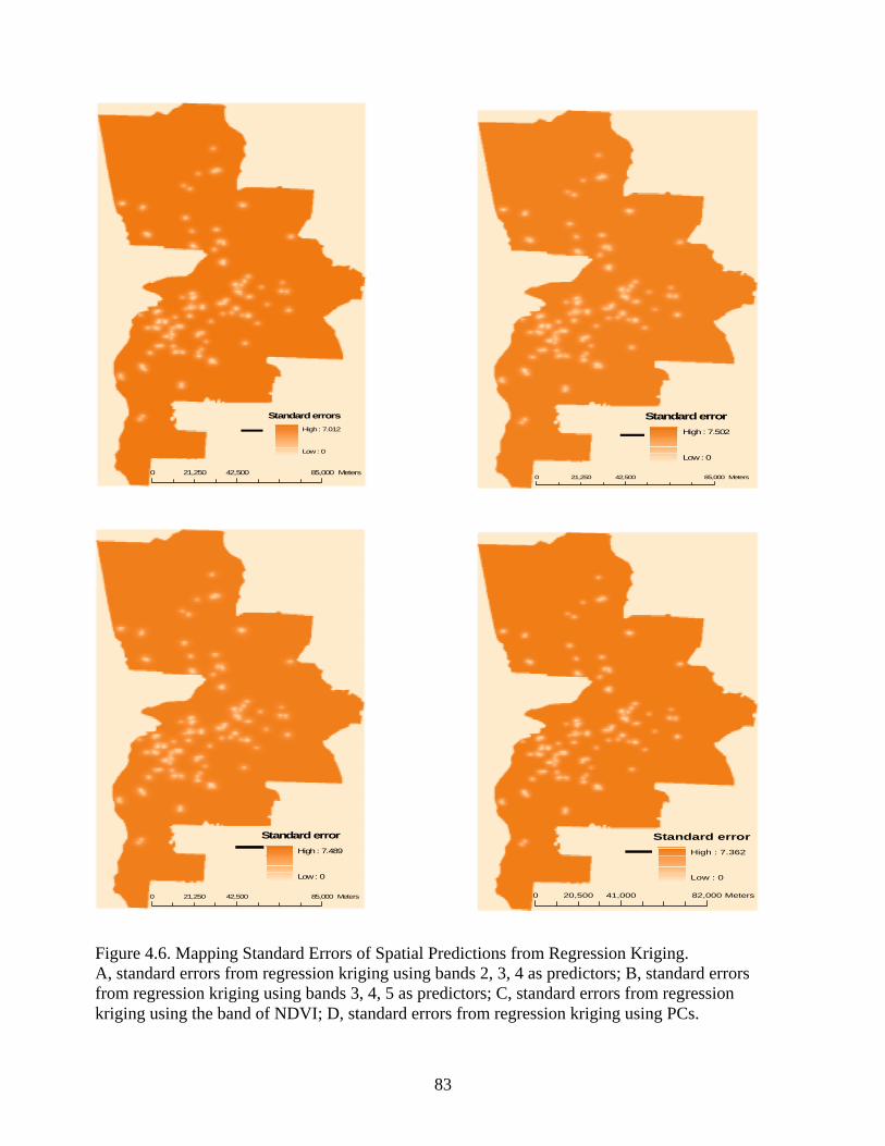
83
Figure 4.6. Mapping Standard Errors of Spatial Predictions from Regression Kriging. A, standard errors from regression kriging using bands 2, 3, 4 as predictors; B, standard errors from regression kriging using bands 3, 4, 5 as predictors; C, standard errors from regression kriging using the band of NDVI; D, standard errors from regression kriging using PCs.
Standard errorHigh : 7.502
Low : 0¯0 42,500 85,00021,250 Meters
Standard errorsHigh : 7.012
Low : 0¯0 42,500 85,00021,250 Meters
Standard errorHigh : 7.489
Low : 0¯0 42,500 85,00021,250 Meters
Standard errorHigh : 7.362
Low : 0¯0 41,000 82,00020,500 Meters
84
Berterretche et al. (2005), Tuominen et al.(2003), and Zhang et al (2004) applied
geostatistical models to estimate forest variables, leaf area index, and classify forest lands based
on remote sensing data. Compared to their studies, multivariable kriging (i.e., RK in this study)
is robust and results in relative smaller errors. Multivariable kriging can be applied for almost all
kinds of forest parameters. Also, either numerical or categorical data can be used in the process
of kriging, i.e., any kind of variable can be used as auxiliary data or predictors.
Remote sensing data and ground inventory data are collected and stored in different data
structures. The discrepancy between remotely sensed data and ground sampling data might be
the source of big errors in forest predictions (Tokola et al. 1996, Gilbert & Lowell 1997). The
ground inventory data are usually collected at the forest plot level or forest stand level. The plot
size may be from several meters to 10 or 20 meters. The stand size may be from 10 meters to
dozens of meters, and the stands are assumed to be homogenous. Therefore, some ground data
may be finer than remote sensing data in spatial resolution, but generally, remote sensing data
has a finer spatial resolution than ground inventory data. This may result in some noise added to
the geostatistical modeling and cause bias errors and mean-absolute errors.
4.7 Conclusions
The systematic approach of geostatistical prediction and mapping developed by
integrating remote sensing, ground inventory, and GPS data provides a new way to spatially
estimate forest parameters using remotely sensed data. It has many applications in forest or
natural resource management. Forest metrics, such as stand density, dominant height, species,

85
stand age, forest health conditions, the probability of forest fire, biomass, carbon, and so on, can
be incorporated in the model. They can be estimated spatially at finer spatial resolution using
remotely sensed data with higher spatial resolution.
Providing finer spatial information is essential for large area timber, biomass, and carbon
budget management and planning. Kriging is an optimum method for spatial interpolation.
Regression kriging is the most powerful one among the different kriging methods in this research.
It was used to predict the pine basal area at 30m for these 20 counties (about 35000 km2) using
only 2822 ground inventory data points. Four groups of independent variables are used in RK.
The 543 band combination resulted in the smallest BE, RMSE, MAE, and had a relatively
smaller SDe. Therefore, Compared with OK, UK and CoK using different auxiliary data, RK
resulted in the smallest BE, RMSE, SDe, and MAE. Regression kriging using the NDVI as the
predictor could be the best method for pine basal area predictions if computation is considered
for large area basal area inventory, since it has only one independent variable and can
significantly reduce computation time as compared with other band combinations. For other
forest parameters, such as dominant height, timber volume, or biomass/carbon, other band
combinations, such as PCs or NDVI need to be applied again to check which will result in better
estimations.
More research is needed to demonstrate whether the geostatistical approach is more or
less efficient than other methods used for large area forest inventory, such as K nearest neighbor
methods using remotely sensed data. This will further demonstrate the efficiency and usefulness
of this geostatistical approach for forest inventory and management.
86
CHAPTER 5
FINE SPATIAL RESOLUTION FOREST INVENTORY
FOR GEORGIA USING WEIGHTED K NEAREST NEIGHBOR METHOD
5.1 Introduction
The nearest neighbor methods represent one of the simplest and most intuitive techniques in
the field of statistical prediction and the field of data mining. The K nearest neighbor method is an
extension of the nearest neighbor method. In the field of statistics the K nearest neighbor method is
a well known, easy, and successful method for discrimination or prediction. In the field of computer
science, the K nearest neighbor method is a powerful instance-based machine-learning algorithm,
and it is a typical method for data mining. In Chapter 3 I explored the two major disadvantages of the
K nearest neighbor method, which are the selection of K and computation cost.
There are two specific techniques that are especially important in the process of
implementing the K nearest neighbor method. The first is distance metrics, and the second is weight
schemes of the K nearest neighbors. In applications of the K nearest neighbor method for forest
inventory, Euclidian distance often is used as the optimal metric without comparing it with other
distance measurements. The average of the values of the K nearest neighbors is then used as the
optimal estimation for the predicted locations. I will therefore explore distance metrics and weight
schemes in detail.
When the weight scheme is added to KNN, the statistic or machine-learning algorithm is
called the weighted K nearest neighbor (WKNN) (Hechenbichler and Schliep 2004). In a general
sense, WKNN and the basic nearest neighbor algorithm can be seen as voting or ensemble
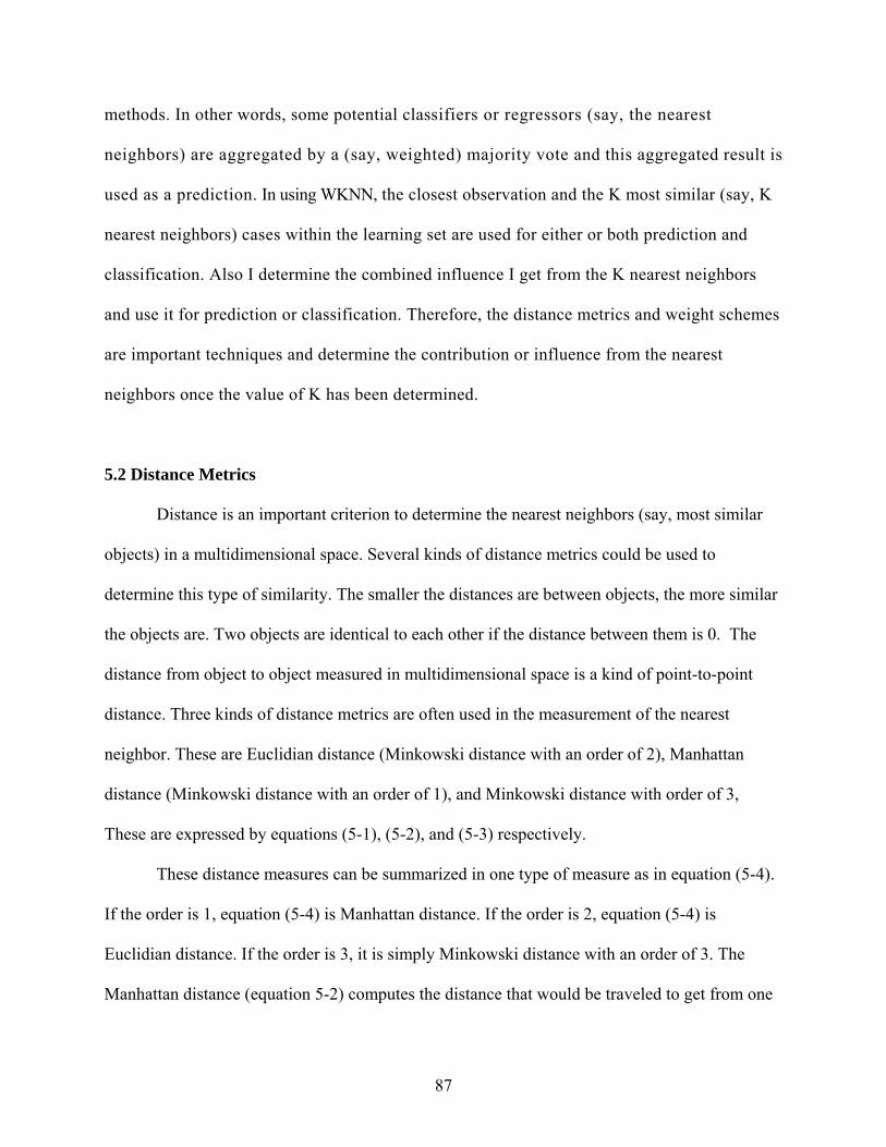
87
methods. In other words, some potential classifiers or regressors (say, the nearest
neighbors) are aggregated by a (say, weighted) majority vote and this aggregated result is
used as a prediction. In using WKNN, the closest observation and the K most similar (say, K
nearest neighbors) cases within the learning set are used for either or both prediction and
classification. Also I determine the combined influence I get from the K nearest neighbors
and use it for prediction or classification. Therefore, the distance metrics and weight schemes
are important techniques and determine the contribution or influence from the nearest
neighbors once the value of K has been determined.
5.2 Distance Metrics
Distance is an important criterion to determine the nearest neighbors (say, most similar
objects) in a multidimensional space. Several kinds of distance metrics could be used to
determine this type of similarity. The smaller the distances are between objects, the more similar
the objects are. Two objects are identical to each other if the distance between them is 0. The
distance from object to object measured in multidimensional space is a kind of point-to-point
distance. Three kinds of distance metrics are often used in the measurement of the nearest
neighbor. These are Euclidian distance (Minkowski distance with an order of 2), Manhattan
distance (Minkowski distance with an order of 1), and Minkowski distance with order of 3,
These are expressed by equations (5-1), (5-2), and (5-3) respectively.
These distance measures can be summarized in one type of measure as in equation (5-4).
If the order is 1, equation (5-4) is Manhattan distance. If the order is 2, equation (5-4) is
Euclidian distance. If the order is 3, it is simply Minkowski distance with an order of 3. The
Manhattan distance (equation 5-2) computes the distance that would be traveled to get from one
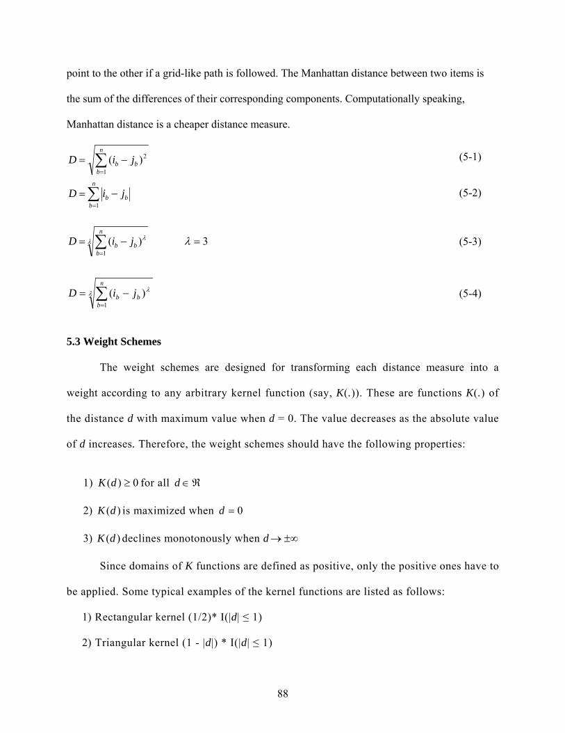
88
point to the other if a grid-like path is followed. The Manhattan distance between two items is
the sum of the differences of their corresponding components. Computationally speaking,
Manhattan distance is a cheaper distance measure.
5.3 Weight Schemes
The weight schemes are designed for transforming each distance measure into a
weight according to any arbitrary kernel function (say, K(.)). These are functions K(.) of
the distance d with maximum value when d = 0. The value decreases as the absolute value
of d increases. Therefore, the weight schemes should have the following properties:
1) 0)( ≥dK for all ℜ∈d
2) )(dK is maximized when 0=d
3) )(dK declines monotonously when d ±∞→
Since domains of K functions are defined as positive, only the positive ones have to
be applied. Some typical examples of the kernel functions are listed as follows:
1) Rectangular kernel (1/2)* I(|d| ≤ 1)
2) Triangular kernel (1 - |d|) * I(|d| ≤ 1)
(5-1) ∑=
−=n
bbb jiD
1
2)(
(5-2) ∑=
−=n
bbb jiD
1
(5-3) λ λ∑=
−=n
bbb jiD
1)( 3=λ
(5-4) λ λ∑=
−=n
bbb jiD
1)(
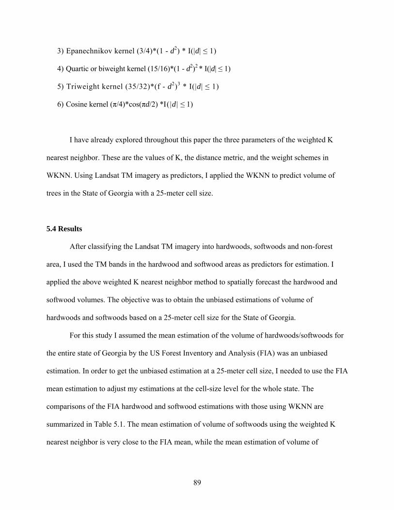
89
3) Epanechnikov kernel (3/4)*(1 - d2) * I(|d| ≤ 1)
4) Quartic or biweight kernel (15/16)*(1 - d2)2 * I(|d| ≤ 1)
5) Triweight kernel (35/32)*(f - d2)3 * I(|d| ≤ 1)
6) Cosine kernel (π/4)*cos(πd/2) *I(|d | ≤ 1)
I have already explored throughout this paper the three parameters of the weighted K
nearest neighbor. These are the values of K, the distance metric, and the weight schemes in
WKNN. Using Landsat TM imagery as predictors, I applied the WKNN to predict volume of
trees in the State of Georgia with a 25-meter cell size.
5.4 Results
After classifying the Landsat TM imagery into hardwoods, softwoods and non-forest
area, I used the TM bands in the hardwood and softwood areas as predictors for estimation. I
applied the above weighted K nearest neighbor method to spatially forecast the hardwood and
softwood volumes. The objective was to obtain the unbiased estimations of volume of
hardwoods and softwoods based on a 25-meter cell size for the State of Georgia.
For this study I assumed the mean estimation of the volume of hardwoods/softwoods for
the entire state of Georgia by the US Forest Inventory and Analysis (FIA) was an unbiased
estimation. In order to get the unbiased estimation at a 25-meter cell size, I needed to use the FIA
mean estimation to adjust my estimations at the cell-size level for the whole state. The
comparisons of the FIA hardwood and softwood estimations with those using WKNN are
summarized in Table 5.1. The mean estimation of volume of softwoods using the weighted K
nearest neighbor is very close to the FIA mean, while the mean estimation of volume of
90
hardwoods is higher than that by FIA. I then applied the ratios of the mean FIA estimation to the
mean WKNN estimation to all estimations at the cell size level for Georgia, and then obtained
the unbiased estimations. In other words, assuming the mean estimation by FIA was an unbiased
estimation, I obtained estimations for hardwood and softwood at the 25-meter cell size using the
weighted K nearest neighbor method. I then used the ratio of the FIA mean to the KNN mean as
a balance index to multiply by my estimations at each cell in a raster dataset. Cieszewski et al
(2003) proofed this approach to obtaining unbiased estimations.
I summarize this fine spatial resolution forest inventory (i.e., the 25-meter cell) to the
county level in Table 5.2. Figures 5.1 and 5.2 display the total volume of hardwoods and
FIA
Mean Total Estimation
Mean Total Ratio of Mean
Softwoods 140.4 503877695 147.4 692269753 0.95 Hardwoods 112.1 536589533 141.9 646415865 0.79 FIA, US Forest Inventory and Analysis Program; Mean is cubic meters per hectare, and Total is cubic meters.
Table 5.1. Simple Comparisons of Volume with the Inventory by FIA
91
softwoods at the county level. These figures generally display the total production of hardwoods
and softwoods. I also display the volume per hectare (i.e., total volume over the area of forest
lands) at the county level, which indicates the production potentials of hardwoods and softwoods
for the 159 counties in Georgia (Figures 5.3 and 5.4). The volume of hardwoods and softwoods
for each county and the relative difference between my estimation and the FIA summarization
also are listed in Table 5.2.
Volume per hectare mapping indicates economic value (i.e., the timber productivity) as
well as value to the ecosystem in the form of biomass and carbon production, which play
important roles in land use dynamics and land resource management. The 30 counties having
high hardwood volume per hectare are aggregated in northern Georgia. Another sub-region, with
4 counties located along the Florida boundary, also has high values of hardwood volume per
hectare. Twenty counties of lower values of hardwood volume per hectare lay like a belt across
central Georgia. There are several other lower values of hardwood volume per hectare counties
in southern Georgia (Figure 5.3).
For spatial distribution of softwood volume per hectare is different in Georgia (Figure
5.4) from that of hardwood. A region of about 20 counties with high values of softwood volume
per hectare exists in south central Georgia. A region of about 20 counties of lower values of
softwood volume per hectare is located in central Georgia. The counties located in northern
Georgia have relatively high values of softwood volume per hectare.
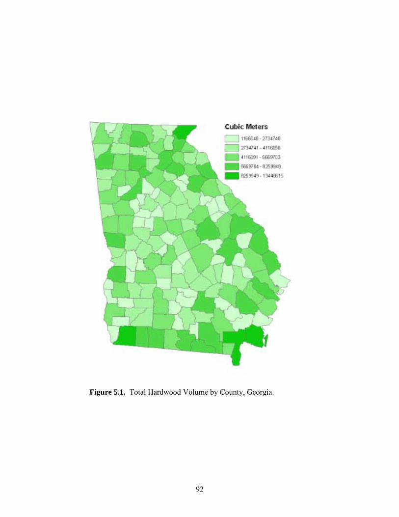
92
Figure 5.1. Total Hardwood Volume by County, Georgia.
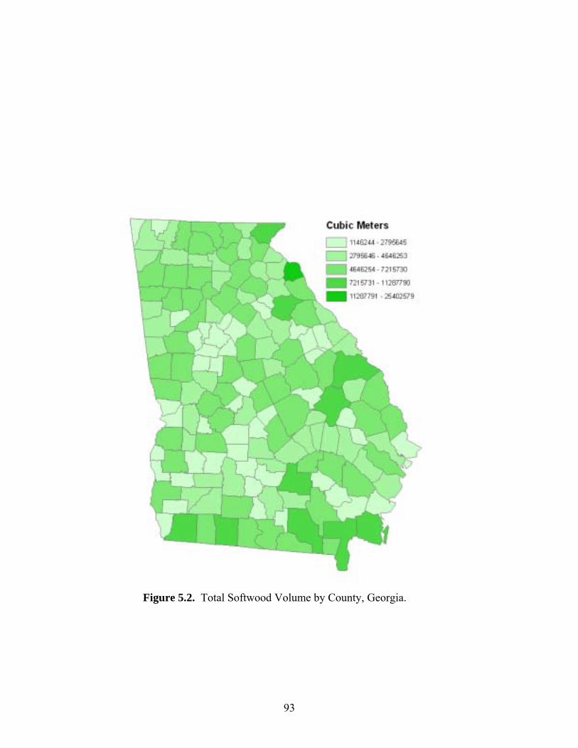
93
Figure 5.2. Total Softwood Volume by County, Georgia.
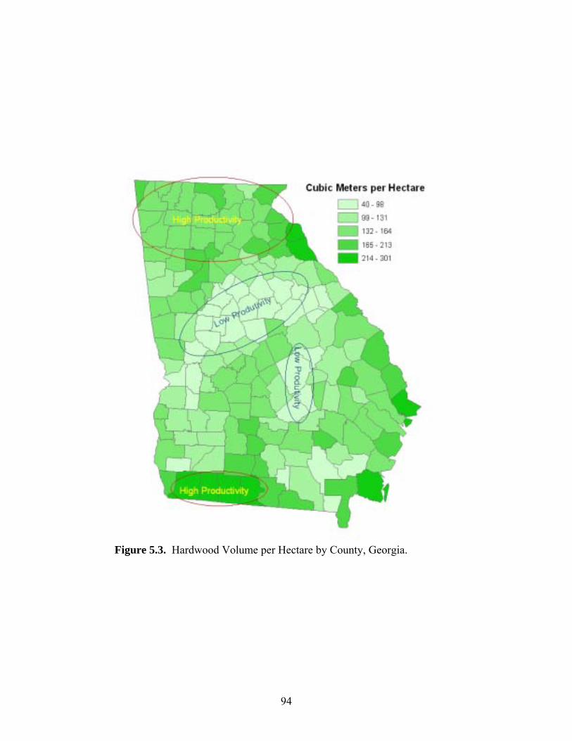
94
Figure 5.3. Hardwood Volume per Hectare by County, Georgia.
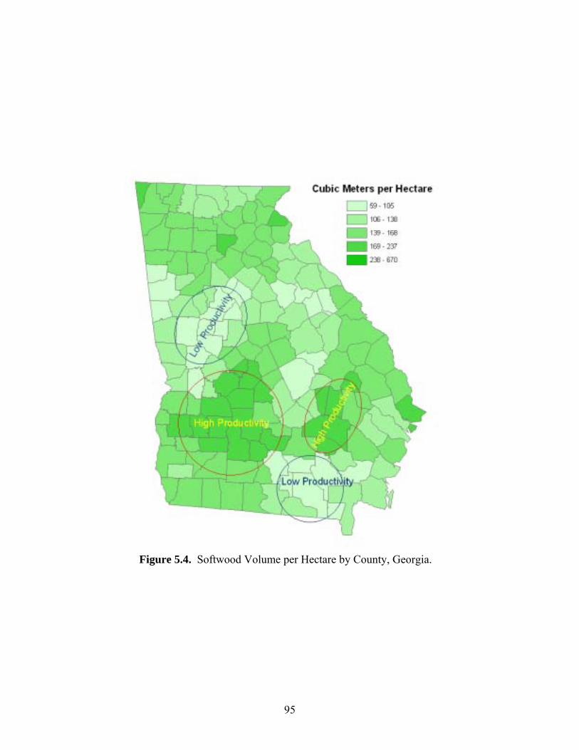
95
Figure 5.4. Softwood Volume per Hectare by County, Georgia.
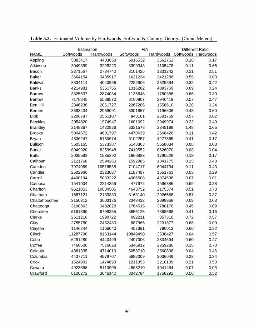
96
Table 5.2. Estimated Volume by Hardwoods, Softwoods, County, Georgia (Cubic Meters).
NAME Estimation
Softwoods Hardwoods FIA
Softwoods Hardwoods Different Ratio
Softwoods HardwoodsAppling 5083417 4403658 6016532 3662752 0.18 0.17Atkinson 3049399 3225220 3399343 1105478 0.11 0.66Bacon 2371567 2734740 3101425 1331242 0.31 0.51Baker 3664154 3435917 1631234 3421286 0.55 0.00Baldwin 3334114 4040996 2282606 2325894 0.32 0.42Banks 4214981 5361755 1316282 4093769 0.69 0.24Barrow 3325637 2874034 1135648 1750386 0.66 0.39Bartow 7178345 5588570 3100807 2940419 0.57 0.47Ben Hill 2846236 2061727 2267286 1556610 0.20 0.24Berrien 3593434 2959091 5301857 1196606 0.48 0.60Bibb 2206787 2551107 943101 2601769 0.57 0.02Bleckley 2054820 1974947 1601092 2949974 0.22 0.49Brantley 2148367 1422828 5331578 2345198 1.48 0.65Brooks 5004572 4601797 4470639 2666426 0.11 0.42Bryan 4336247 5130674 6102257 4277365 0.41 0.17Bulloch 5603165 5373387 5143303 5558034 0.08 0.03Burke 8049920 8259948 7419552 8626070 0.08 0.04Butts 2035593 1535292 1666883 1790529 0.18 0.17Calhoun 2121768 2594260 1592985 1341775 0.25 0.48Camden 7974059 10518535 7104717 6044734 0.11 0.43Candler 2502960 2323087 1187487 1651763 0.53 0.29Carroll 4400194 5033222 4086508 4974538 0.07 0.01Catoosa 1541004 2214359 477972 1596386 0.69 0.28Charlton 9521053 10034505 4643752 2175374 0.51 0.78Chatham 1687121 2139339 3163140 2926558 0.87 0.37Chattahoochee 2150312 3003126 2348432 2899968 0.09 0.03Chattooga 3190863 3482028 1764515 3788176 0.45 0.09Cherokee 6161890 6798385 3656125 7888668 0.41 0.16Clarke 2511216 1990722 692211 857316 0.72 0.57Clay 2755780 2452430 887965 2231877 0.68 0.09Clayton 1146244 1166040 457391 790013 0.60 0.32Clinch 11287790 8163144 10849490 3538427 0.04 0.57Cobb 6291280 4440499 2497006 2334694 0.60 0.47Coffee 7466600 7576623 6346912 2259286 0.15 0.70Colquitt 4881335 4714019 5058710 2560838 0.04 0.46Columbia 4437711 4579707 5682009 3036049 0.28 0.34Cook 1524902 1474893 1211353 2210139 0.21 0.50Coweta 4923558 5110905 4563210 4941464 0.07 0.03Crawford 6126272 3646142 3042784 1758292 0.50 0.52
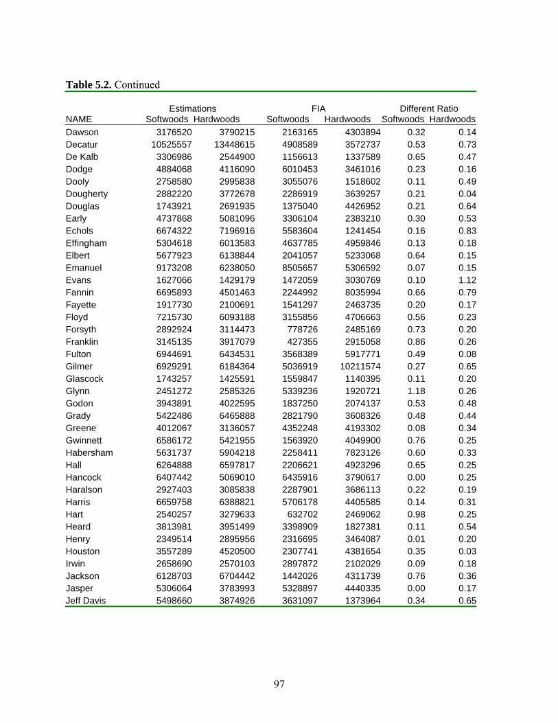
97
Table 5.2. Continued
NAME Estimations
Softwoods Hardwoods FIA
Softwoods Hardwoods Different Ratio
Softwoods HardwoodsDawson 3176520 3790215 2163165 4303894 0.32 0.14Decatur 10525557 13448615 4908589 3572737 0.53 0.73De Kalb 3306986 2544900 1156613 1337589 0.65 0.47Dodge 4884068 4116090 6010453 3461016 0.23 0.16Dooly 2758580 2995838 3055076 1518602 0.11 0.49Dougherty 2882220 3772678 2286919 3639257 0.21 0.04Douglas 1743921 2691935 1375040 4426952 0.21 0.64Early 4737868 5081096 3306104 2383210 0.30 0.53Echols 6674322 7196916 5583604 1241454 0.16 0.83Effingham 5304618 6013583 4637785 4959846 0.13 0.18Elbert 5677923 6138844 2041057 5233068 0.64 0.15Emanuel 9173208 6238050 8505657 5306592 0.07 0.15Evans 1627066 1429179 1472059 3030769 0.10 1.12Fannin 6695893 4501463 2244992 8035994 0.66 0.79Fayette 1917730 2100691 1541297 2463735 0.20 0.17Floyd 7215730 6093188 3155856 4706663 0.56 0.23Forsyth 2892924 3114473 778726 2485169 0.73 0.20Franklin 3145135 3917079 427355 2915058 0.86 0.26Fulton 6944691 6434531 3568389 5917771 0.49 0.08Gilmer 6929291 6184364 5036919 10211574 0.27 0.65Glascock 1743257 1425591 1559847 1140395 0.11 0.20Glynn 2451272 2585326 5339236 1920721 1.18 0.26Godon 3943891 4022595 1837250 2074137 0.53 0.48Grady 5422486 6465888 2821790 3608326 0.48 0.44Greene 4012067 3136057 4352248 4193302 0.08 0.34Gwinnett 6586172 5421955 1563920 4049900 0.76 0.25Habersham 5631737 5904218 2258411 7823126 0.60 0.33Hall 6264888 6597817 2206621 4923296 0.65 0.25Hancock 6407442 5069010 6435916 3790617 0.00 0.25Haralson 2927403 3085838 2287901 3686113 0.22 0.19Harris 6659758 6388821 5706178 4405585 0.14 0.31Hart 2540257 3279633 632702 2469062 0.98 0.25Heard 3813981 3951499 3398909 1827381 0.11 0.54Henry 2349514 2895956 2316695 3464087 0.01 0.20Houston 3557289 4520500 2307741 4381654 0.35 0.03Irwin 2658690 2570103 2897872 2102029 0.09 0.18Jackson 6128703 6704442 1442026 4311739 0.76 0.36Jasper 5306064 3783993 5328897 4440335 0.00 0.17Jeff Davis 5498660 3874926 3631097 1373964 0.34 0.65
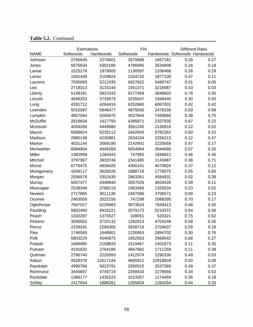
98
Table 5.2. Continued
NAME Estimations
Softwoods Hardwoods FIA
Softwoods Hardwoods Different Ratio
Softwoods HardwoodsJohnson 2795645 2276601 3570696 1657181 0.28 0.27Jones 5675634 4352180 4789485 3534908 0.16 0.19Lamar 1525178 1879005 1130597 1336468 0.26 0.29Lanier 1591448 2109824 2334720 1877109 0.47 0.11Laurens 7030069 5212435 6927622 5489747 0.01 0.05Lee 2718313 3133144 1551371 3219087 0.43 0.03Liberty 5148181 5922343 9177459 3848603 0.78 0.35Lincoln 4646253 3733679 3235647 1848440 0.30 0.50Long 4391712 4264416 6252860 6067001 0.42 0.42Lowndes 5015587 5846477 4879266 2478158 0.03 0.58Lumpkin 4857084 4265875 3027844 7459994 0.38 0.75McDuffie 2618834 1917750 4385871 2337935 0.67 0.22McIntosh 4059266 4449580 3561245 2135816 0.12 0.52Macon 6088824 5235112 2442943 5782362 0.60 0.10Madison 2980148 4230881 2634234 2256213 0.12 0.47Marion 4031144 2669190 2142901 2225659 0.47 0.17Meriwether 6084904 4949269 5654964 3944686 0.07 0.20Miller 1382958 1264343 747950 1846812 0.46 0.46Mitchell 3797967 3933746 2341485 1143487 0.38 0.71Moroe 6776475 4639425 4300141 4070624 0.37 0.12Montgomery 4209117 3526026 1888718 1778075 0.55 0.50Morgan 2936578 3302430 2863361 4584931 0.02 0.39Murray 5007477 4348840 3057029 4828426 0.39 0.11Muscogee 2536349 2768119 1963366 1328534 0.23 0.52Newton 2717865 3011136 2467586 3706571 0.09 0.23Oconee 2463059 2522156 747299 2088280 0.70 0.17Oglethorpe 7647027 6226983 3973524 7849413 0.48 0.26Paulding 5802460 4915221 2079173 5219372 0.64 0.06Peach 1332297 1370527 339051 520321 0.75 0.62Pickens 3056552 3720132 1282013 4704248 0.58 0.26Pierce 2239241 2294305 3558719 2704637 0.59 0.18Pike 1746569 1648801 1230953 2894702 0.30 0.76Polk 5803229 4040875 1852563 2968542 0.68 0.27Pulaski 1699980 2158833 1519467 1401673 0.11 0.35Putnam 4191632 2764186 4667982 1711259 0.11 0.38Quitman 2786740 2229393 1412974 2290330 0.49 0.03Rabun 9328378 12017244 4665912 10918604 0.50 0.09Randolph 4990766 5623791 2550515 3537369 0.49 0.37Richmond 3445657 4749719 2258433 2278556 0.34 0.52Rockdale 1366177 1435223 1013357 1174459 0.26 0.18Schley 2417654 1888281 1355834 1264264 0.44 0.33
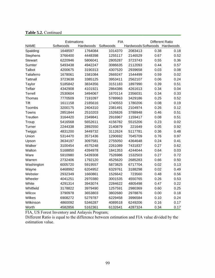
99
Table 5.2. Continued
NAME Estimations
Softwoods Hardwoods FIA
Softwoods HardwoodsDifferent Ratio
Softwoods HardwoodsSpalding 1648597 1764084 1014370 2083413 0.38 0.18Stephens 3766400 4448398 1255117 2146529 0.67 0.52Stewart 6220946 5806041 2805287 3723743 0.55 0.36Sumter 5493438 4942247 3086635 2112093 0.44 0.57Talbot 4200675 3190313 4307520 2939658 0.03 0.08Taliaferro 1678061 1581084 2669247 1544499 0.59 0.02Tattnall 3723638 3385125 3953411 2562107 0.06 0.24Taylor 5185842 3834356 3151183 1897990 0.39 0.51Telfair 4342908 4101921 2864386 4261613 0.34 0.04Terrell 2530604 3494067 1670114 2356031 0.34 0.33Thomas 7770509 7191097 5789963 3429186 0.25 0.52Tift 1611158 2185616 1740553 1780206 0.08 0.19Toombs 3200175 2404310 2381491 2104974 0.26 0.12Towns 2851844 2510203 1526826 3788948 0.46 0.51Treutlen 3164420 2349841 2916967 1159417 0.08 0.51Troup 5416568 5652611 4156782 5515206 0.23 0.02Turner 2244338 2892550 2140879 221649 0.05 0.92Twiggs 4831200 3449732 3112624 5117781 0.36 0.48Union 5314470 3571436 1290692 7045709 0.76 0.97Upson 3634197 3097581 2755050 4364648 0.24 0.41Walker 3100454 4575248 2261089 7431837 0.27 0.62Walton 5168850 4394978 1841353 4244044 0.64 0.03Ware 5910980 5439308 7526986 1532503 0.27 0.72Warren 2732406 1792120 4525620 2685283 0.66 0.50Washington 6005720 5919557 5873825 6717704 0.02 0.13Wayne 6468992 6204952 6329761 3188298 0.02 0.49Webster 2932349 1660861 1526642 723560 0.48 0.56Wheeler 4041251 2970380 3001535 4550765 0.26 0.53White 4291314 3943074 2284622 4805498 0.47 0.22Whitfield 3178822 3979490 1257591 2980369 0.60 0.25Wilcox 3790978 3653803 3802680 2978876 0.00 0.18Wilkes 6908272 5279787 6229458 3996584 0.10 0.24Wilkinson 4860092 5346287 4089518 6249206 0.16 0.17Worth 4582856 5162361 6132641 4287324 0.34 0.17FIA, US Forest Inventory and Anlaysis Program; Different Ratio is equal to the difference between estimation and FIA value divided by the estimation value.
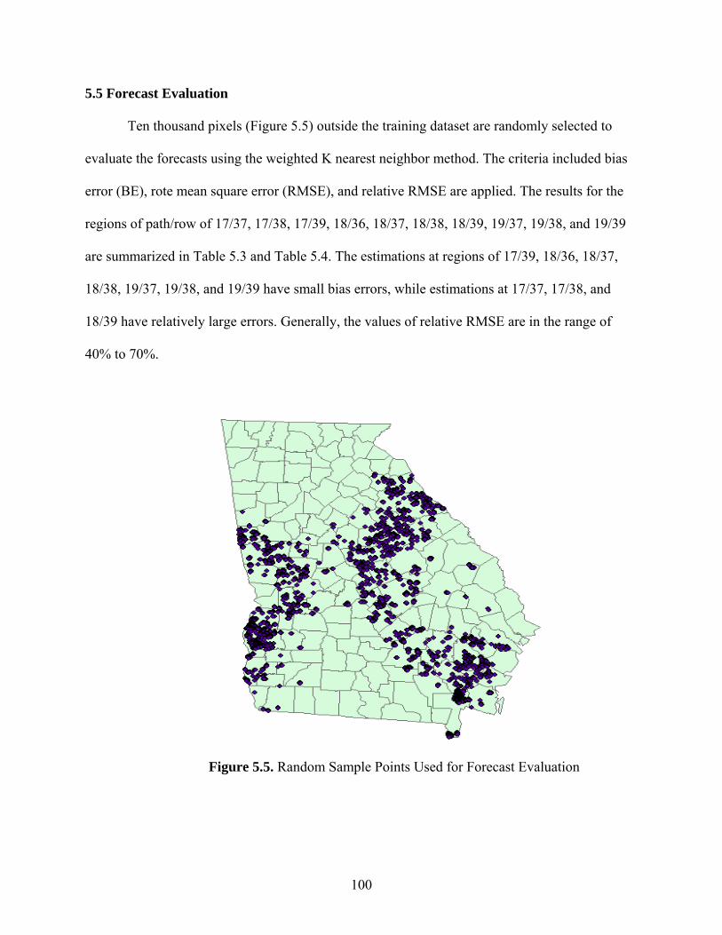
100
5.5 Forecast Evaluation
Ten thousand pixels (Figure 5.5) outside the training dataset are randomly selected to
evaluate the forecasts using the weighted K nearest neighbor method. The criteria included bias
error (BE), rote mean square error (RMSE), and relative RMSE are applied. The results for the
regions of path/row of 17/37, 17/38, 17/39, 18/36, 18/37, 18/38, 18/39, 19/37, 19/38, and 19/39
are summarized in Table 5.3 and Table 5.4. The estimations at regions of 17/39, 18/36, 18/37,
18/38, 19/37, 19/38, and 19/39 have small bias errors, while estimations at 17/37, 17/38, and
18/39 have relatively large errors. Generally, the values of relative RMSE are in the range of
40% to 70%.
Figure 5.5. Random Sample Points Used for Forecast Evaluation
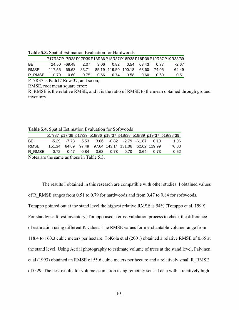
101
Table 5.3. Spatial Estimation Evaluation for Hardwoods P17R37 P17R38 P17R39 P18R36 P18R37 P18R38 P18R39 P19R37 P19R38/39 BE 24.50 -69.48 2.07 3.06 0.82 0.54 63.43 0.77 -2.67 RMSE 117.55 69.63 83.71 85.19 119.50 100.18 63.60 74.05 64.49 R_RMSE 0.79 0.60 0.75 0.56 0.74 0.58 0.60 0.60 0.51 P17R37 is Path17 Row 37, and so on; RMSE, root mean square error; R_RMSE is the relative RMSE, and it is the ratio of RMSE to the mean obtained through ground inventory. Table 5.4. Spatial Estimation Evaluation for Softwoods p17r37 p17r38 p17r39 p18r36 p18r37 p18r38 p18r39 p19r37 p19r38r39 BE -5.29 -7.73 5.53 3.06 -0.82 -2.79 -61.87 0.10 1.06 RMSE 151.34 64.69 97.49 97.64 143.14 131.06 62.02 119.99 76.00 R_RMSE 0.72 0.47 0.84 0.63 0.78 0.70 0.64 0.73 0.52 Notes are the same as those in Table 5.3. The results I obtained in this research are compatible with other studies. I obtained values
of R_RMSE ranges from 0.51 to 0.79 for hardwoods and from 0.47 to 0.84 for softwoods.
Tomppo pointed out at the stand level the highest relative RMSE is 54% (Tomppo et al, 1999).
For standwise forest inventory, Tomppo used a cross validation process to check the difference
of estimation using different K values. The RMSE values for merchantable volume range from
118.4 to 160.3 cubic meters per hectare. ToKola et al (2001) obtained a relative RMSE of 0.65 at
the stand level. Using Aerial photography to estimate volume of trees at the stand level, Paivinen
et al (1993) obtained an RMSE of 55.6 cubic meters per hectare and a relatively small R_RMSE
of 0.29. The best results for volume estimation using remotely sensed data with a relatively high
102
spatial resolution still have a high RMSE and a high R_RMSE. For example, the best results
using JETS-1 (Japanese Earth Resources Satellite-1 with 18 m resolution) have an RMSE of 60
cubic meters per hectare (Schemullius et al 2005); while Tomppo et al (1995) using ERS SAR
(i.e., European Space Agency, Synthetic Aperture Radar) images to estimate volume achieved an
RMSE of 90 cubic meters per hectare and an R_RMSE of 0.584. In my research, the study unit is
25-m, and the RMSE for hardwood is in the range of 63.6 to 119.5, and RMSE of softwoods is in
the range of 62.02 to 151.34. Reese et al (2003) conducted a countywide forest inventory, and
reported the R_RMSE values are 0.58, 0.59, 0.66, and 0.69 at selected areas; they also listed the
values of RMSE in Remniingstorp (e.g. a test region in Sweden) as 21, 32, 52, 87, 109, and 159
cubic meters per hectare.
However, most of the study areas in the previously mentioned publications are smaller
than my study area. They usually used one scene or a small part of a scene of Landsat imagery,
and the forest types in their study areas are simple. For example, the forest species in northern
Europe are relatively more uniform compared to forests in the southern US. The study area in the
research conducted by Tomppo et al is 1000 ha (1999), and ToKola et al used parts of one scene
of Landsat imagery (2001). Using Landsat TM data to predict volume typically will result in
relatively low accuracy at the pixel level (Tomppo 1993, Mouer and Stage 1995, ToKola et al
1996) yet relatively high accuracy for large areas such as the stand or landscape level (Franklin
1986, Poso et al 1987, Ahern et al 1991). It is also of significance that when trees become
mature, the volume increases but the canopy closes, while the relationship between spectral
reflectance and wood volume can be asymptotic and relationships for those higher volumes
become less accurate. Therefore, in the applications of Landsat TM imagery, there is limited
information content for denser and older forests.
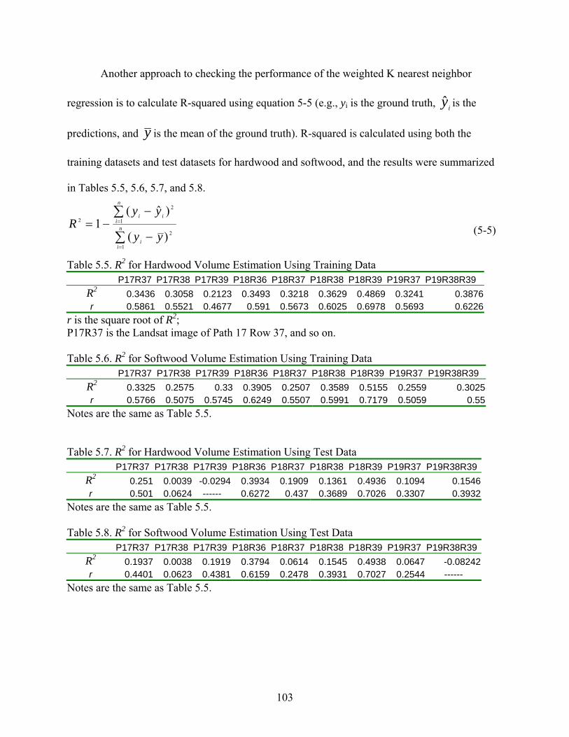
103
Another approach to checking the performance of the weighted K nearest neighbor
regression is to calculate R-squared using equation 5-5 (e.g., yi is the ground truth, iy is the
predictions, and y is the mean of the ground truth). R-squared is calculated using both the
training datasets and test datasets for hardwood and softwood, and the results were summarized
in Tables 5.5, 5.6, 5.7, and 5.8.
Table 5.5. R2 for Hardwood Volume Estimation Using Training Data P17R37 P17R38 P17R39 P18R36 P18R37 P18R38 P18R39 P19R37 P19R38R39
R2 0.3436 0.3058 0.2123 0.3493 0.3218 0.3629 0.4869 0.3241 0.3876r 0.5861 0.5521 0.4677 0.591 0.5673 0.6025 0.6978 0.5693 0.6226
r is the square root of R2; P17R37 is the Landsat image of Path 17 Row 37, and so on. Table 5.6. R2 for Softwood Volume Estimation Using Training Data P17R37 P17R38 P17R39 P18R36 P18R37 P18R38 P18R39 P19R37 P19R38R39
R2 0.3325 0.2575 0.33 0.3905 0.2507 0.3589 0.5155 0.2559 0.3025r 0.5766 0.5075 0.5745 0.6249 0.5507 0.5991 0.7179 0.5059 0.55
Notes are the same as Table 5.5. Table 5.7. R2 for Hardwood Volume Estimation Using Test Data P17R37 P17R38 P17R39 P18R36 P18R37 P18R38 P18R39 P19R37 P19R38R39
R2 0.251 0.0039 -0.0294 0.3934 0.1909 0.1361 0.4936 0.1094 0.1546r 0.501 0.0624 ------ 0.6272 0.437 0.3689 0.7026 0.3307 0.3932
Notes are the same as Table 5.5. Table 5.8. R2 for Softwood Volume Estimation Using Test Data P17R37 P17R38 P17R39 P18R36 P18R37 P18R38 P18R39 P19R37 P19R38R39
R2 0.1937 0.0038 0.1919 0.3794 0.0614 0.1545 0.4938 0.0647 -0.08242r 0.4401 0.0623 0.4381 0.6159 0.2478 0.3931 0.7027 0.2544 ------
Notes are the same as Table 5.5.
∑
∑
=
=
−
−−= n
ii
n
iii
yy
yyR
1
2
1
2
2
)(
)ˆ(1 (5-5)
104
The R2 values calculated using training datasets were bigger than those using test
datasets. The smaller the errors in the estimated wood volume, the bigger are the R2 values.
Therefore, the predictions using images of Path 18 Row 36 and Path 18 Row 39 have smaller
errors, while the inventories using other images have relatively big errors. The R2 values using
images Path 17 Row 38 and Path 17 Row 39 for hardwood volume inventory were close to 0
(Tables 5.7), which indicates big errors in the estimations. For softwood inventory using K
nearest neighbor regression, the R2 values using images Path 17 Row 38 and Path 19 Row 38 and
39 were close to 0, and there were big errors in the estimations. The performance of the K
nearest neighbor regression was also indicated using scatter plots of predictions versus
observations for hardwood and softwood volume using both training datasets and test datasets
(Figures 5.6, 5.7, 5.8, and 5.9).
5.6 Conclusions
Using the FIA mean estimation of volume, I adjusted the estimations using the weighted
K nearest neighbor method and obtained the unbiased estimations. I then summarized the
estimations for hardwoods and softwoods by county for the state of Georgia. I assessed total
volume and mean volume of hardwoods and softwoods at the county level and identified the
regions with high and low volume per hectare in Georgia. Volume per hectare also is an
important indication for forest ecosystems in the state of Georgia. Using 10,000 random pixels, I
evaluated my estimations, and compared these assessments with other available studies. This
research is compatible with other studies.
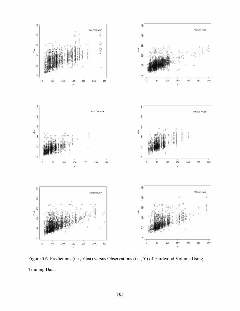
105
Figure 5.6. Predictions (i.e., Yhat) versus Observations (i.e., Y) of Hardwood Volume Using
Training Data.
Y
Yhat
0 50 100 150 200 250 300
050
100
150
200
250
Path17Row37
Y
Yhat
0 50 100 150 200 250 300
050
100
150
200
250
Path17Row38
Y
Yhat
0 50 100 150 200 250 300
050
100
150
200
250
Path17Row39
Y
Yha
t
0 50 100 150 200 250 300
050
100
150
200
250
Path18Row36
Y
Yhat
0 50 100 150 200 250 300
050
100
150
200
250
Path18Row37
Y
Yhat
0 50 100 150 200 250 300
050
100
150
200
250
Path18Row38
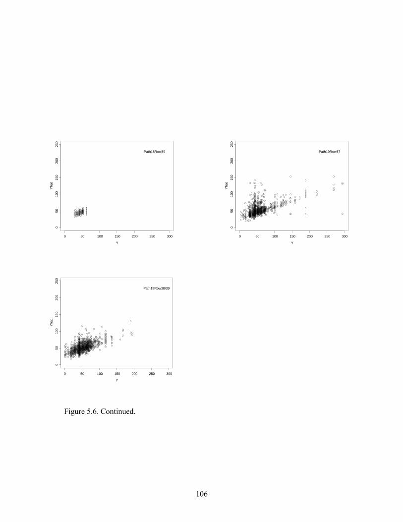
106
Y
Yha
t
0 50 100 150 200 250 300
050
100
150
200
250
Path18Row39
Y
Yha
t
0 50 100 150 200 250 3000
5010
015
020
025
0
Path19Row37
Y
Yhat
0 50 100 150 200 250 300
050
100
150
200
250
Path19Row38/39
Figure 5.6. Continued.
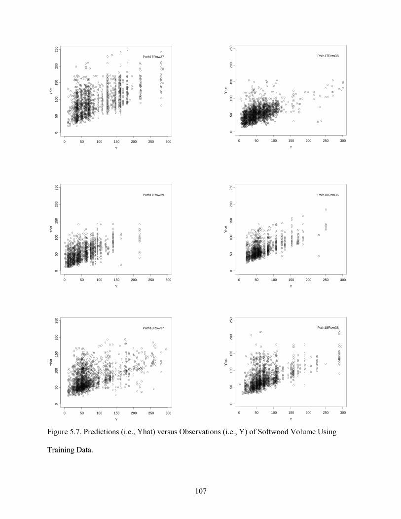
107
Figure 5.7. Predictions (i.e., Yhat) versus Observations (i.e., Y) of Softwood Volume Using
Training Data.
Y
Yhat
0 50 100 150 200 250 300
050
100
150
200
250
Path17Row37
Y
Yhat
0 50 100 150 200 250 300
050
100
150
200
250
Path17Row38
Y
Yhat
0 50 100 150 200 250 300
050
100
150
200
250
Path17Row39
Y
Yhat
0 50 100 150 200 250 300
050
100
150
200
250
Path18Row36
Y
Yhat
0 50 100 150 200 250 300
050
100
150
200
250
Path18Row37
Y
Yhat
0 50 100 150 200 250 300
050
100
150
200
250
Path18Row38
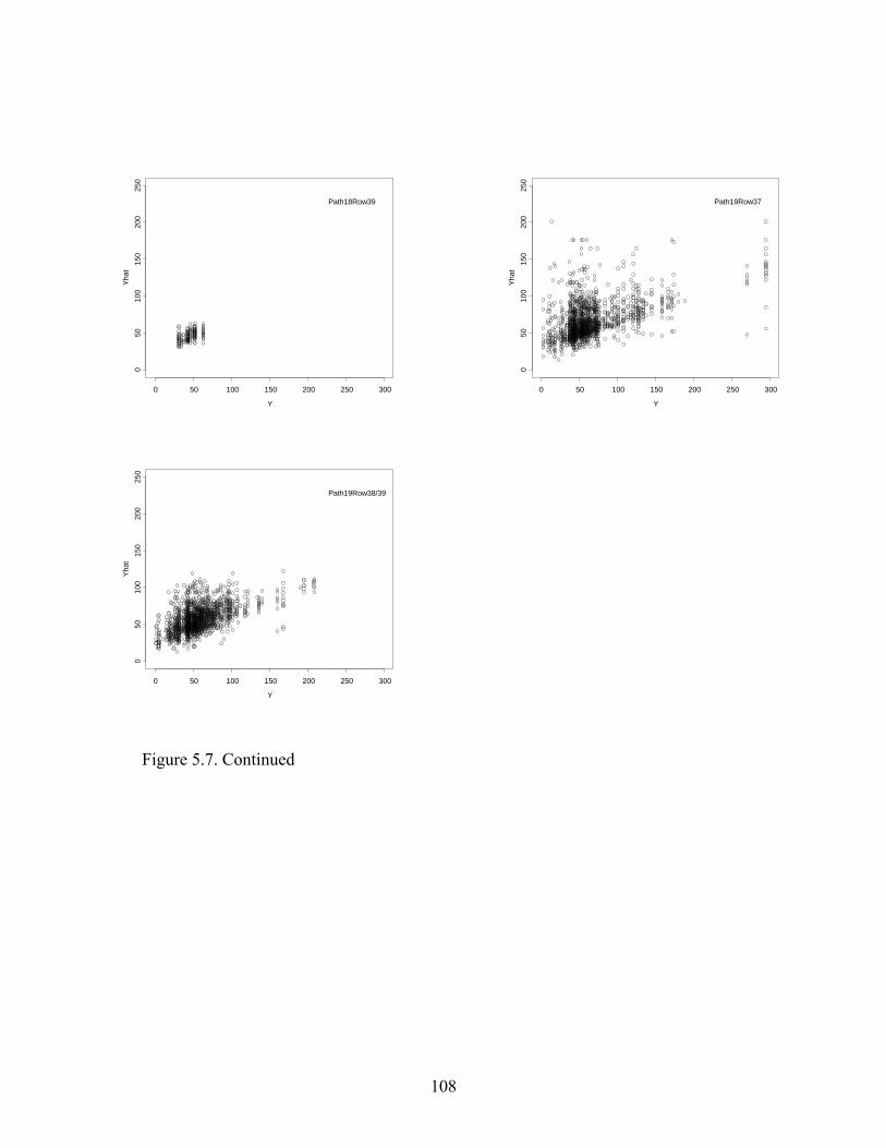
108
Y
Yhat
0 50 100 150 200 250 300
050
100
150
200
250
Path18Row39
Y
Yhat
0 50 100 150 200 250 300
050
100
150
200
250
Path19Row37
Y
Yhat
0 50 100 150 200 250 300
050
100
150
200
250
Path19Row38/39
Figure 5.7. Continued
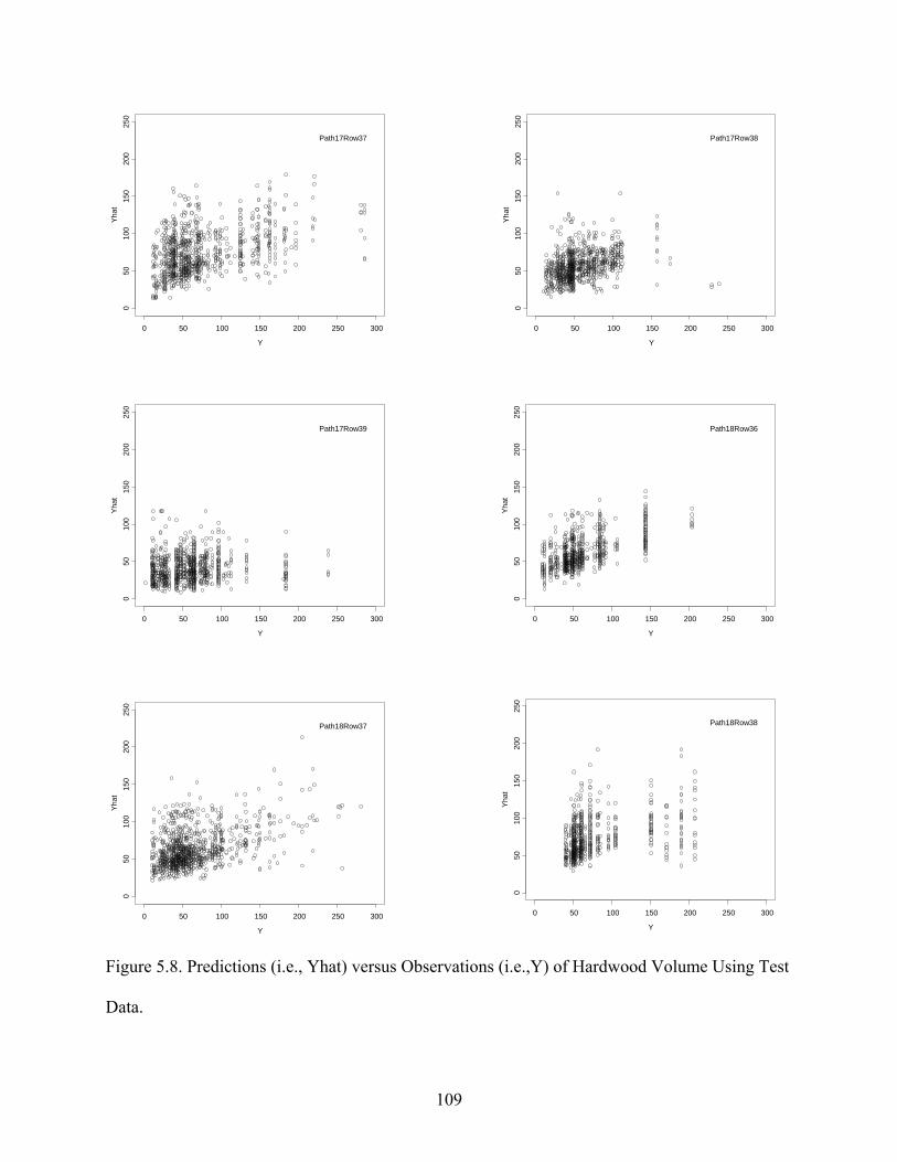
109
Figure 5.8. Predictions (i.e., Yhat) versus Observations (i.e.,Y) of Hardwood Volume Using Test
Data.
Y
Yhat
0 50 100 150 200 250 300
050
100
150
200
250
Path17Row38
Y
Yhat
0 50 100 150 200 250 300
050
100
150
200
250
Path17Row39
Y
Yhat
0 50 100 150 200 250 300
050
100
150
200
250
Path18Row36
Y
Yhat
0 50 100 150 200 250 300
050
100
150
200
250
Path18Row38
Y
Yhat
0 50 100 150 200 250 300
050
100
150
200
250
Path18Row37
Y
Yhat
0 50 100 150 200 250 300
050
100
150
200
250
Path17Row37
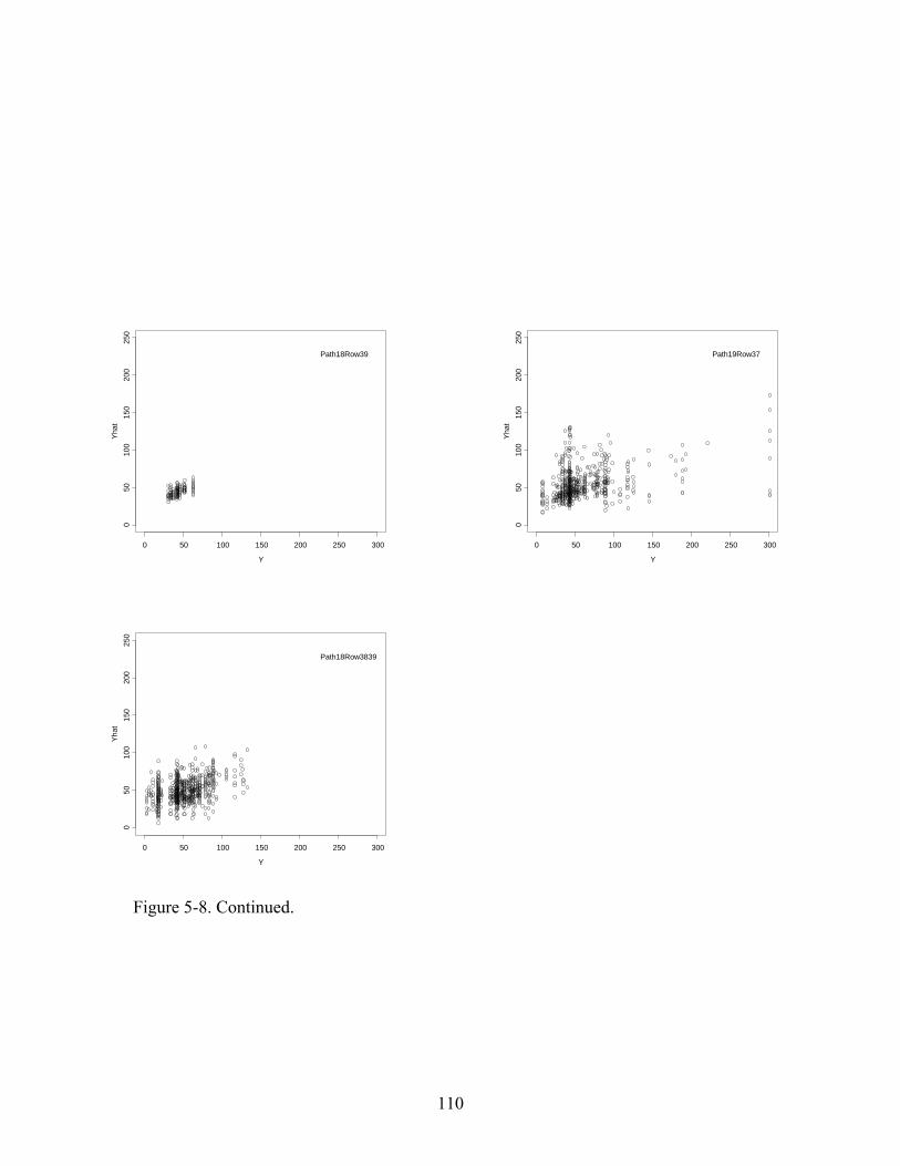
110
Y
Yhat
0 50 100 150 200 250 300
050
100
150
200
250
Path19Row37
Y
Yhat
0 50 100 150 200 250 300
050
100
150
200
250
Path18Row39
Y
Yhat
0 50 100 150 200 250 300
050
100
150
200
250
Path18Row3839
Figure 5-8. Continued.
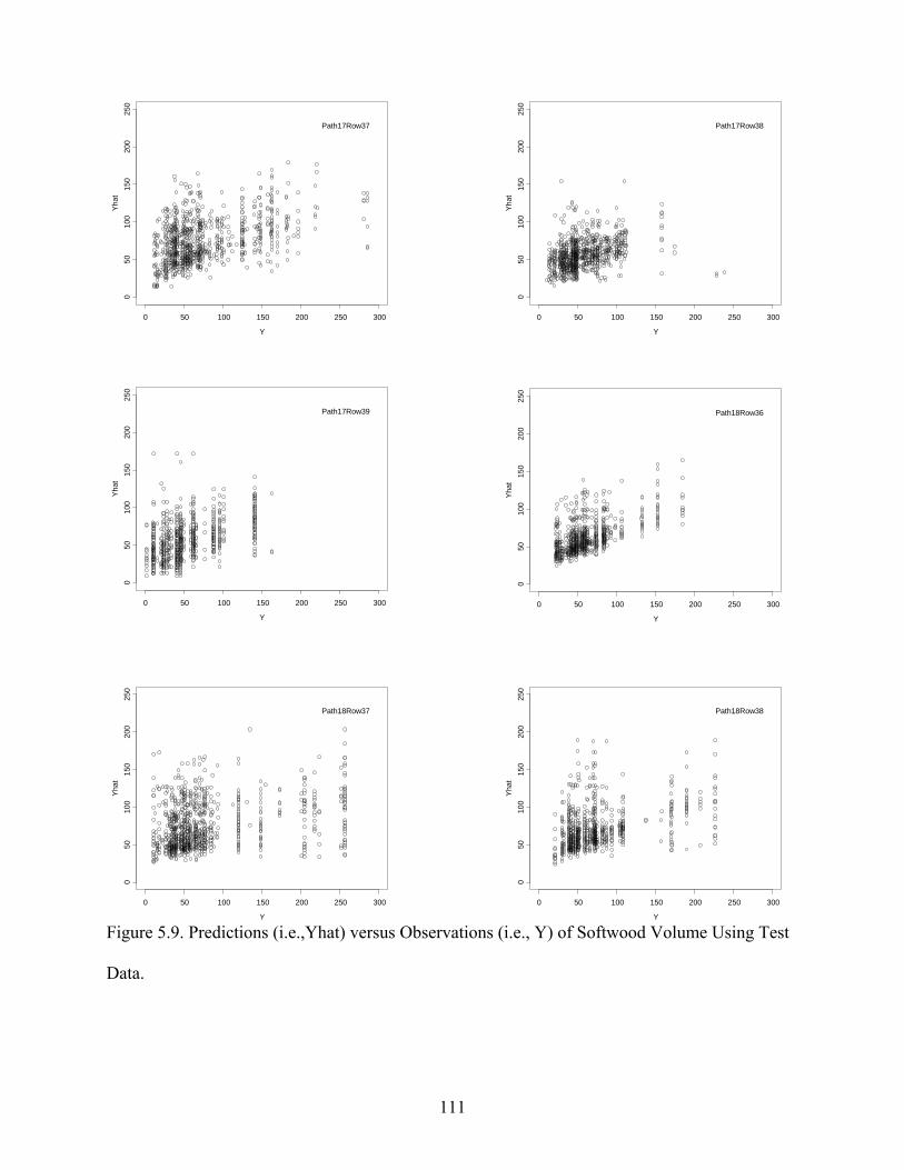
111
Figure 5.9. Predictions (i.e.,Yhat) versus Observations (i.e., Y) of Softwood Volume Using Test
Data.
Y
Yhat
0 50 100 150 200 250 300
050
100
150
200
250
Path17Row38
Y
Yhat
0 50 100 150 200 250 300
050
100
150
200
250
Path18Row36
Y
Yhat
0 50 100 150 200 250 300
050
100
150
200
250
Path17Row39
Y
Yhat
0 50 100 150 200 250 300
050
100
150
200
250
Path18Row37
Y
Yhat
0 50 100 150 200 250 300
050
100
150
200
250
Path18Row38
Y
Yhat
0 50 100 150 200 250 300
050
100
150
200
250
Path17Row37
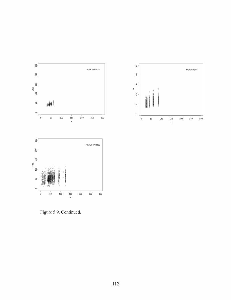
112
Y
Yhat
0 50 100 150 200 250 300
050
100
150
200
250
Path18Row39
Y
Yhat
0 50 100 150 200 250 300
050
100
150
200
250
Path19Row37
Y
Yhat
0 50 100 150 200 250 300
050
100
150
200
250
Path19Row3839
Figure 5.9. Continued.
113
CHAPTER 6
CONCLUSION AND DISCUSSION
6.1 Conclusions
The objective of this research is to develop and apply a remote sensing based approach
for large area forest inventory in order to estimate forest variables with fine spatial resolution
(i.e., a 25-m cell size). The K nearest neighbor method is a popular method and is widely applied
for forest inventory. However, current research of applying K nearest neighbor method for forest
inventory overlooks some of its disadvantages.
Forest is one of the main geographical phenomena, and its attributes have a typical
geographical characteristic, spatial dependence. Therefore, a geostatistical approach is developed
so that forest variables can be predicted using these spatial BLUP methods, i.e., a group of
kriging methods.
Four sub-objectives are addressed in order to obtain the main objective of fine spatial
resolution forest inventory. First, a powerful approach based on the nearest neighbor algorithm is
developed to remove cloud and cloud shadow from the Landsat images so that the Landsat
imagery can be applied as predictors for forest inventory. Second, two disadvantages of K
nearest neighbor method is explored. The selection of K values is improved using statistical tests
and comparisons of cumulative distribution functions. The computation cost can be reduced
using remote sensing data reduction methods while the most useful information is still
maintained in the reduced dataset. Third, a systematic geostatistical approach is developed for
forest inventory. This approach includes spatial/aspatial data exploration, semivriogram
114
modeling, and kriging modeling. The kriging modeling typically includes ordinary kriging,
universal kriging, Cokriging, and regression kriging. Regression kriging is the robust one that
can incorporate both the correlation between predictors and response variables and the spatial
association between predictors and response variables. Regression kriging takes advantages of
regression and kriging. Fourth, for K nearest neighbor method, I explored the distance metrics
and weight schemes. The estimations of K nearest neighbor are improved using improved
distance measurements and weight schemes.
Finally, I use the weighted K nearest neighbor method to forecast volume of hardwoods
and softwoods for each 25-meter pixel across the whole state of Georgia. The estimations are
adjusted using the FIA unbiased mean estimate in order to obtained unbiased estimation. The
estimates are then summarized at county level. Spatial patterns of forest productivity are
characterized using the hardwood and softwood volume per hectare.
6.2 Contributions and Limitations
This study makes several contributions to forest biometrics, natural resources
management, and GIS research. First, remote sensing based up-to-date forest inventory for the
state of Georgia (i.e., state level or larger regions) with fine spatial resolution can be achieved
using geostatistcal modeling or the K nearest nearest neighbor method in a short time.
Geostatistical modeling needs the basic assumption that the variables applied in the models
should be random variables, while there is no assumption for the K nearest neighbor method.
Second, a systematic geostatistical approach is developed and explored in detail for forest
inventory. This geostatistical approach extends from the methods of ordinary and universal
kriging that are applied in the current studies to Cokriging and regression kriging using remote
115
sensing imagery as predictors. The geostatistical approach developed in this research, as one of
the main geospatial technologies, can be applied for any type of natural resources management
including timber, wildlife, range, recreation, and hazards.
Third, the disadvantage of K nearest neighbor (i.e., the selection of K) is addressed using
statistical methods. Typically, using 2 or 3 nearest neighbors resulted in good estimations since a
large value of K in application of K nearest neighbor for prediction will result in relatively
smooth spatial estimations of forest variables, while spatial variability is lost. Additionally, I
develop a SAS program and extend the K nearest neighbor method for remote sensing data
preprocessing, i.e., cloud and cloud shadow removal from Landsat TM imagery. The results
indicate that nearest neighbor is a powerful method for removing clouds and cloud shadows in
Landsat images, and this method can be applied for preprocessing other types of remote sensing
imagery.
There are some limitations of this research. First, the accuracy of inventory estimates
obtained in this work needs improving. Although it is compatible with other studies for forest
inventory and its results are adjusted to the unbiased estimation, its accuracy is rather low.
Second, the estimations at county level are obtained using remote sensing (i.e., Landsat TM
imagery) and modeling. The applications of these results to a specific county need additional
ground truthing and finer resolution data, for example up-to-date aerial photos. Third, there is not
an integrated automatic approach for forest inventory using either the geostatistical approaches
or K nearest neighbor method developed and applied in this research. Applying these approaches
requires use of ArcGIS, Leica Geosystems ERDAS Imagine, ENVI, SAS, Splus and R
programming.

116
6.3 Further Study
Combining Landsat TM imagery with other higher spatial resolution data can improve
the accuracy of spatial estimations. One type higher spatial resolution data is Quick Bird, and
using one scene of Landsat TM image as an example is a practicable approach. This way will
significantly increase the data size. Therefore, the next question to be solved is to develop fast
computation algorithms for processing remote sensing data.
Another interesting step is to understand the difference between the estimations and FIA
values at county level. There are obvious errors in the FIA data. For example, the land area of
softwoods for county Catoosa is 0, while the volume of softwoods is 477971 cubic meters.
Maybe this error resulted from typos in the process of data input by FIA staff. There are certain
uncertainties in the estimations using K nearest neighbor method. Using geospatial simulation
and trying to understand the uncertainty in the predictions also are meaningful.
117
REFERENCES
Anselin, L. 1995. Local indicators of spatial association – LISA. Geographical Analysis, 27: 93-115.
Ahern, F.J., Erdle, T., Maclean, D.A. and I.D. Kneppeck. 1991. A quantitative relationship
between forest growth rates and Thematic Mapper reflectance measurements. International Journal of Remote Sensing, 12:387-400.
Arana, E., P. Delicado, L. and Marti-Bonmati. 2005. Validation procedures in radiological
diagnostic models, neural network and logistic regression. Http://www.econ.upf.es/deehome/what/wpapers/postscripts/414.pdf. Accessed on August 2, 2006.
Ardö, J. 1992. Volume quantification of coniferous forest compartments using spectral radiance
recorded by Landsat Thematic Mapper. International Journal of Remote Sensing, 13: 1779-1786.
Atkinson, P.M. and P. Lewis. 2000. Geostatistical classification for remote sensing: an
introduction. Computers & Geosciences, 26: 361-371. Atkinson, P.M., Webster, R. and P.J. Curran. 1994. Cokriging with airborne MSS imagery.
Remote Sensing of Environment, 50: 335-345. Atkinson, P. M. 1993. The effect of spatial resolution on the experimental variogram of
airborne MSS imagery. International Journal of Remote Sensing, 14: 1005–1011.
Atta-Boateng, J. and J.W.M. Jr. 1998. A method for classifying commercial tree species of an uneven-aged mixed species tropical forest for growth and yield model construction. Forest Ecology and Management, 104: 89-99.
Baath, H., Andreas Gallerspang Goran Hallsby, Lundstrom, A., Lofgren, P., Nillsson, M. and
Goran Zstahl. Remote sensing, field survey, and long-term forescasting: an efficient combination for local assessments of forest fuels. Biomass and Bioenergy, 22:145-147.
Barnsley, M.J. 1999. Digital remote sensing data and their characteristics, In: Paul A. Longley,
Michael F. Goodchild, David J. Maguire and David (Eds) Geographical Information Systems: Principles, Techniques, Applications, and Management, John Wiely & Sons: New Jersey.
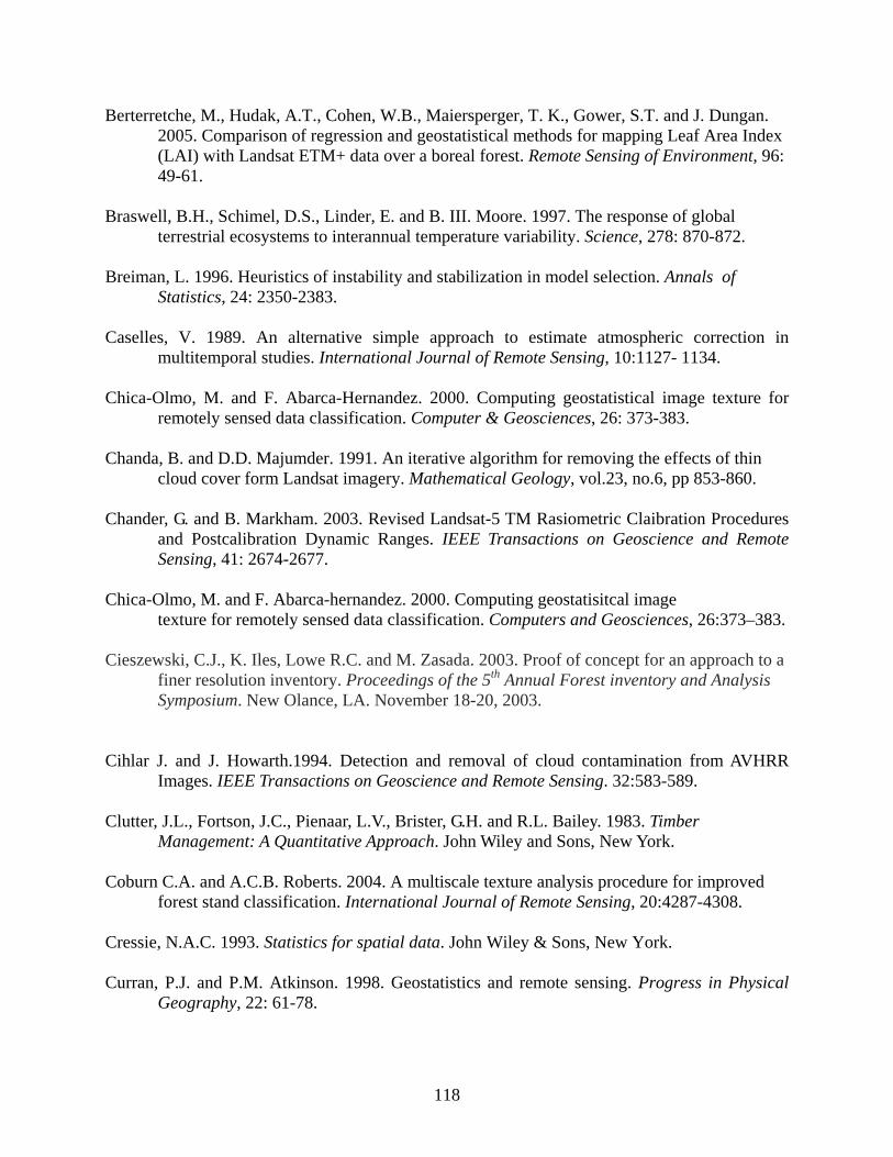
118
Berterretche, M., Hudak, A.T., Cohen, W.B., Maiersperger, T. K., Gower, S.T. and J. Dungan. 2005. Comparison of regression and geostatistical methods for mapping Leaf Area Index (LAI) with Landsat ETM+ data over a boreal forest. Remote Sensing of Environment, 96: 49-61.
Braswell, B.H., Schimel, D.S., Linder, E. and B. III. Moore. 1997. The response of global
terrestrial ecosystems to interannual temperature variability. Science, 278: 870-872. Breiman, L. 1996. Heuristics of instability and stabilization in model selection. Annals of
Statistics, 24: 2350-2383. Caselles, V. 1989. An alternative simple approach to estimate atmospheric correction in
multitemporal studies. International Journal of Remote Sensing, 10:1127- 1134. Chica-Olmo, M. and F. Abarca-Hernandez. 2000. Computing geostatistical image texture for
remotely sensed data classification. Computer & Geosciences, 26: 373-383. Chanda, B. and D.D. Majumder. 1991. An iterative algorithm for removing the effects of thin
cloud cover form Landsat imagery. Mathematical Geology, vol.23, no.6, pp 853-860. Chander, G. and B. Markham. 2003. Revised Landsat-5 TM Rasiometric Claibration Procedures
and Postcalibration Dynamic Ranges. IEEE Transactions on Geoscience and Remote Sensing, 41: 2674-2677.
Chica-Olmo, M. and F. Abarca-hernandez. 2000. Computing geostatisitcal image
texture for remotely sensed data classification. Computers and Geosciences, 26:373–383.
Cieszewski, C.J., K. Iles, Lowe R.C. and M. Zasada. 2003. Proof of concept for an approach to a finer resolution inventory. Proceedings of the 5th Annual Forest inventory and Analysis Symposium. New Olance, LA. November 18-20, 2003.
Cihlar J. and J. Howarth.1994. Detection and removal of cloud contamination from AVHRR
Images. IEEE Transactions on Geoscience and Remote Sensing. 32:583-589. Clutter, J.L., Fortson, J.C., Pienaar, L.V., Brister, G.H. and R.L. Bailey. 1983. Timber
Management: A Quantitative Approach. John Wiley and Sons, New York. Coburn C.A. and A.C.B. Roberts. 2004. A multiscale texture analysis procedure for improved
forest stand classification. International Journal of Remote Sensing, 20:4287-4308. Cressie, N.A.C. 1993. Statistics for spatial data. John Wiley & Sons, New York. Curran, P.J. and P.M. Atkinson. 1998. Geostatistics and remote sensing. Progress in Physical
Geography, 22: 61-78.
119
Curran, P.J. 1988. The semivariogram in remote sensing: an introduction. Remote Sensing of Envrironment, 24: 493-507.
Czaplewski, R.L., Reich, R.M. and Bechtold, W.A. 1994. Spatial autocorrelation in growth of
undisturbed natural pine stands across Georgia. Forest Science, 40:314-328. Curran P.J. and P.M. Atkinson.1998. Geostatistics and remote sensing. Progress in Physical Geography, 22:61-78. Dungan, J.L., Peterson, D.L. and P.J. Curran. 1994. Alternative approaches for mapping
vegetation quantities using ground and image data. In: Michener, W., Stafford, S. & Brunt, J. (eds.). Environmental information management and analysis: ecosystem to global scales. Taylor and Francis, London, UK. pp. 237-261.
Dungan, J.L. 1998. Spatial prediction of vegetation quantities using ground and image data.
International Journal of Remote Sensing, 19: 267-285. Efron B, and R. Tibshirani. 1997. Cross-validation and the bootstrap: Estimating the error rate of
a prediction rule. Journal of the American Statistical Association, 92:548-560. Fazakas, Z. and M. Nilsson. 1996. Volume and forest cover estimation voer southern Sweden
using AVHRR data calibrated with TM data. International Journal of Remote Sensing, 17:1701-1709.
Franklin, J. 1986. Thematic Mapper analysis of coniferous forest structure and composition.
International Journal of Remote Sensing, 7: 1287-1301. Foody, G.M. and D.S. Boyd. 1999. Fuzzy mapping of tropical land cover along an
environmental gradient from remotely sensed data with an artificial neural network. Journal of Geographical Systems, 1: 23-35
Foody, G.M. 2000. Mapping land cover from remotely sensed data with a softened feed forward
neural network classification. Journal of Intelligent and Robotic Systems, 29: 433-449. Fotheringham A. S. and P. Rogerson. 1994. Spatial Analysis and GIS, London: Taylor and
Francis, Ch.2, pp.25-27, Franco-Lopez, Ek, A.R. and M.E. Bauer. 2001. Estimation of forest stand density, volume, and
cover type using the K-nearest neighbors method. Remote Sensing of Environment, 77: 251-274.
Gilbert, B. and K. Lowell. 1997. Forest attributes and spatial autocorrelation and interpolation:
effects of alternative sampling schemata in the boreal forest. Landscape and Urban Planning, 37: 235-244.
Goodchild, M.F. 2004. The validity and usefulness of laws in geographic information science
and geography. Annals of the Association of American Geographers, 94: 284–289.
120
Goodchild M. F.2003.
Http://www.csiss.org/aboutus/presentations/files/goodchild_ucgis_jun03.pdf. University of California, Santa Barbara.
Goovaerts, P. 1997. Geostatistics for natural resources evaluation. Oxford University Press,
New York. Goward, S.N., Tucker, C.J. and D.G. Dye. 1985. North American vegetation patterns observed
with the NOAA-7 advanced very high resolution radiometer. Vegetatio, 64: 3-14. Gunnarsson, F., Holm, S., Holmgren, P., and T. Thuresson. 1998. On the potential of kriging for
forest management planning. Scand. J. For. Res. 13: 237–245. Hardin P.J. and C.N. Thomson. 1992. Fast Nearest Neighbor Classification Methods for
Multispectral Imagery. Professional Geographer, 44: 191-201. Hastie, T., Tibshirani, R. and J. Friedman. 2001. The Elements of Statistical Learning: Data
Mining, Inference, and Prediction. New York: Springer press. 415-420 p. Hechenbichler K. and K.P. Schliep. 2004. Weighted k-Nearest-Neighbor Techniques and
Ordinal Classification. http://www.stat.uni-muenchen.de/sfb386/papers/dsp/paper399.ps. Accessed on October 15, 2006.
Heikkila, J., Nevalainen, S. and T. Tokola. 2002. Estimating defoliationin borealconiferous
forests by combining Landsat TM, aerial photographs and field data. Forest Ecology and Mangement 158:9-23
Hock, B.K., Payn, T.W. and J.W. Shirley. 1993. Uisng a geographic information system and
geostatistics to estimate site index of Pinus radiata for Kaingaroa Forest. New Zealand. N. Z. J. For. Sci., 23:264-277.
Holmström, H. and J.E.S. Fransson. 2003. Combining remotely sensed optical and radar data in
kNN estimation of forest variables. Forest Science, 10: 409-418. Holmstrom, H. 2002. Estimation of single-tree characteristics using the KNN method and
plotwise aerial photograph interpretations. Forest Ecology and Management, 167:303-314.
Holmstrom, H. 2002. Estimation of single-tree characteristics using the KNN method and
plotwise aerial photograph interpretations Forest Ecology and Management, 167:303-314.
121
Holmgren, P. and T. Thuresson. 1997. Applying objectively estimated and spatially continuous forest parameters in tactical planning to obtain dynamic treatment units. Forest Science, 43:317-326.
Holmgren, J., Joyce, S., Nilsson, M. and H. Olsson. 2000. Estimating stem volume and basal
area in forest compartments b combining satellite image data with field data. Scandinavian Journal of Forest Research, 15:103-111.
ITT Company. ENVI Add-Ons FLAASH. http://www.ittvis.com/envi/flaash.asp. Accessed on
July 28, 2006. James M. 1985. Classification Algorithms. New York: John Wiley & Sons. 168 p. Jensen, J.R. 1986. Introductory Digital Image Processing: A Remote Sensing Perspective.
Englewood Cliffs, NJ: Prentice-Hall. 151-169 p. Journel, A. G., Kyriakidis, P.C. and S. Mao. 2000. Correcting the Smoothing Effect of
Estimators: A Spectral Postprocessor. Mathematical Geology, 32: 787-813. Jupp, D. B., Strahler, A. H. and C. E. Woodcock. 1988. Autocorrelation and
regularization in digital images I. Basic theory. IEEE Transactions on Geoscience and Remote Sensing, 26: 463–473.
Kramer, E. Conroy, M.J., Anderson, E.A. Bumback, W.R. and J. Epstein. 2003. The Geogorgia Gap Analysis Project. Institute of Ecology and Georgia Cooperative Fish & Wildlife Research Unit, University of Georgia.
Katila, M. and E. Tomppo. 2002. Stratification by ancillary data in mutisource forest inventries
employing k-nearest-neighbour estimation. Canadian Journal of Forest Research, 32:1548-1561.
Katila, M., Heikkinen, J. and E. Tomppo. 2000. Calibration of small-area estimation for map
errors in multisource forest inventory. Canadian Journal of Forest Research, 30:1329-1339.
Katila, M., E. Tomppo. 2001. Selecting estimation parameters for the Finnish Mulisource
national forest inventory. Remote Sensing of Environment, 76:16-32. Kleinn, C. New technologies and methodologies for national forest inventories.
http://www.fao.org/docrep/005/y4001e/Y4001E03.htm. Accessed on November 22, 2006.
Lark, R. M. 1996. Geostatistical description of texture on an aerial photograph for
discriminating classes of land cover. International Journal of Remote Sensing, 17, 2115–2133.
122
Liu Z.K. and B.R. Hunt. 1984.A new approach to removing cloud cover from satellite imagery. Computer vision, Graphics, and Image Processing, 25: 252-25.
Matheron, G. 1965. Les Variable Regionalisees et leur Estimation. Masson, Paris. McRoberts, R.E., Nelson, M.D. and D.G. Wendt. 2002. tratified estimation of forest area using
satellite imagery, inventory data, and the K-nearest neighbor technique. Remote Sensing of Environment, 82:457-468.
Meng, Q. and C.J. Cieszewski. 2006. Spatial variability and cluster analysis of tree mortality.
Physical Geography, (In press). Miller, H.J. 2004. Tobler’s First Law and Spatial Analysis. Annals of the Association of
American Geographers, 94: 284–289. Mitchell, O.R., Delp, E.J. and P.L.Chen. 1977. Filtering to remove cloud cover in satellite
Imagery. IEEE Transactions on Geoscience Electronics, Vol. GE-15, no.3, pp. 137-141. Moeur, M. and A.R. Stage. 1995. Most similar neighbor: an improved sampling inference
procedure for natural resource planning. Forest Science, 41:337-359. Myers, D.E. 1982. Matrix formulation of cokriging. Mathematic Geology, 14: 249-157. Myers, B. 1996. Http://www.ai-geostats.org/archives/1996/AI-11-96/0039.html. Accessed on
May 1, 2006. Myneni R.B., C.D. Keeling, C.J. Tucker, Asrar, G. and R.R. Nemani. 1997. Increased plant
growth in the northern high latitudes from 1981 to 1991. Nature, 386: 698-702.
Murphy, A.H. and R.W. Katz. 1985. Probability, Statistics, and Decision Making in the Atmospheric Sciences. Boulder, Colo: Westview Press.
Nanos, N. and G. Montero. 2002. Spatial prediction of diameter distribution models. For. Ecol.
Manage. 161: 147–158. Nanos N., Calama R., Montero G., and L. Gil. 2004. Geostatistical prediction of height/diameter
models. Forest Ecology and Management, 195: 221-235. Odeh, I.O.A., McBratney, A.B. and D.J. Chittleborough. 1995. Further results on prediction of
soil properties from terrain attributes: heterotopic cokriging and regression-kring. Geoderma, 67: 215-226.
Odeh, I.O.A. and A.B. McBratnery. 2000. Using AVHRR images for spatial prediction of clay
content in the lower Namoi Valley of eastern Australia. Geoderma, 97: 237-245.
123
Paivinen, R., Pussinen, A. and E. Tomppo. 1993. Assessment of boreal forest stands using field assessment and remote senign, Proceedings of Earsel Conference. ITC Enshedene, the Netherlands. Aprial 19-23, 1993.
Pebesma, E. J. 2004. Multivariable Geostatistics in S: the Gstat Package. Computer &
Geosciences, 30: 683-691. Pebesma, E.J. 2005. The Gstat Package. http://cran.r-project.org/doc/packages/gstat.pdf.
Accessed on November 25, 2005. Poso, S., Paananen, R. and M. Simila 1987. Forest inventory by compartments using satellite
imagery, Silva Fennica, 21: 69-94. Reese, H., Nilsson, M., Pahlen, T.G., Hagner, O., Joyce, S., Tingelof, U., Egberth, M. and H.
Olsson. 2003. Countywide estimation of forest variables using satellite data and field data from the national forest inventory. AMBIO, 32: 542-548.
Reese, H., Nilsson, M., Sandstrom, P. and H. Olsson. 2002. Applications using estimates of
forest parameters derived from satellite and forest inventory data. Computers and Electronics in Agriculture, 37:37-55.
Samra, J.S., Gill, H.S. and V.K. Bhatia. 1989. Spatial stochastic modeling of growth and forest
resource evaluation. Forest Science, 35:663-676. Shao, J. and D. Tu. 1995. The Jackknife and Bootstrap, New York: Springer-Verlag. Short, N.M. 1999. The remote sensing tutorial.
Http://www.fas.org/irp/imint/docs/rst/Sect3/Sect3_1.html. Accessed on May 1, 2005. Simonett, D. S. 1983. Theory, instruments, and techniques. Vol. 1 of Manual of Remote
Sensing. Falls Church, VA: American Society of Photogrammetry, p170. Simpson J.J. and J.R. Stitt. 1998. A procedure for the detection and removal of cloud shadow
form AVHRR data over land. IEEE Transactions on Geoscience and Remote Sensing, 36: 880-897.
Song, M. and D.L. Civco. 2002. A knowledge-based approach for reducing cloud and shadow.
ASPRS-ACSM Annual Conference and FIG XXII Congress, April 22-26. Schmullius C. Lecture 4 Introducing to Modeling.
http://earth.esa.int/dragon/Schmullius4_SAR_Introduction_to_Modelling.PDF. Accessed on Nov.11, 2006.
Tatem, A.J., Lewis, H.G., Atkinson, P.M. and Nixon, M.S. 2001. Land cover mapping from
remotely sensed images at the sub-pixel scale using a Hopfield neural network. IEEE Transactions on Geoscience and Remote Sensing, 39: 781-796.
124
Tobler, W. R. 1970. A computer movie simulating urban growth in the Detroit region. Economic Geography, 46: 234–40.
Tobler, W. 2004. On the first law of geography: a reply. Annals of the Association of American
Geographers, 94: 304–310. Tokola, T., Pitkänen, S., Partinen, S. and E. Muinonen. 1996. Point accuracy of a non-parametric
method in estimation of forest characteristics with different satellite materials. International Journal of Remote Sensing, 17: 2333-2351.
Tokola, T. 2000. The influence of field sample data location on growing stock volume estimation
in Landsat TM-based forest inventory in eastern Finland. Remote Sensing of Environment, 74:422-431.
Tokola, T., Pitkanen, J., Partinens, S. and E. Muinonen. 1996. Point accuracy of a non-
parametric method in estimation of forest characteristics with different satellite materials. International Journal of Remote Sensing, 17:2333-2351.
Tomppo, E. 1991. Satellite imagery-based national inventory of Finland. International Archives
of Photogrammetry and Remote Sensing, 28: 419-424. Tomppo, E. 1993. Multi-source national forest inventory of Finland. In: Proceedings of Ilvessalo
Symposium on National Forest Inventories, August 17-21, Finland. pp. 52-59. Tomppo, E., Goulding, C. and M. Katila. 1999. Adapting Finnish multi-source forest inventory
techniques to the New Zealand preharvest inventory. Scandinavian Journal of Forest Resaearch, 14:182-192.
Tomppo, E., Nilsson, M., Rosengren, M., Aalto, P. and P. Kennedy. 2002. Simultaneous use of
Landsat-TM and IRS-1C WIFS data in estimating large area tree stem volume and aboveground biomass. Remote Sensing of Environment, 82:156-57.
Tomppo E. and M. Halme. 2004. Using coarse scale forest variables as ancillary information and
weighting of variables in K-NN estimation: a genetic algorithm approach. Remote Sensing of Environment, 92: 1–20.
Tomppo E., Mikkela, P., Veijanen, A., Makisara, K., Henttone, H., Katila, M., Pullianinen, J.,
Hallikainen, M. and J. Hyyppa. 1995. Application of ERS_1 SAR data in large area forest inventory. Proceedings of the Second ERS Applicatioins Workshop, London, UK. December 6-8, 1995.
Trotter, C.M., Dymond, J.R. and C.J. Goulding. 1997. Estimation of timber volume in a
coniferous plantation forest using Landsat TM. International Journal of Remote Sensing, 18: 2209-2223.
Tucker, C.J. 1979. Red and photographic infrared linear combinations for monitoring vegetation.
Remote Sensing of Environment, 8: 127-150.
125
Tuominen, S., Fish, S. and S. Poso. 2002. Combining remote sensing, data from earlier
inventories, and geostatistical interpolation in multisource forest inventory. Canadian Journal of Forest Research, 33: 624–634.
Tuominen, S., Fish, S. and S. Poso. 2003. Combining remote sensing, data from earlier
inventories, and geostatistical interpolation in multisource forest inventories. Canadian Journal of Forest Research, 33: 623-634
Tuominen, S., Fish, S. and S. Poso. 2003. Combining remote sensing, data from earlier
inventories, and geostatistical interpolation in multisource forest inventory. Canadian Journal of Forest Research, 33:624-634.
Wackernagel, H. 1994. Multivariate spatial statistics. Geoderma, 62: 83-92. Warren, B.C., Spies, T.A. and G.A. Bradshaw. 1990. Semivariograms of digital imagery for
analysis of conifer canopy structure. Remote Sensing of Environment 34: 167-178. Woodcock, C. E., Strahler, A. H. and Jupp, D. 1988a. The use of variograms in remote
sensing: I. Scene models and simulated images. Remote Sensing of Environment, 25: 323–348.
Woodcock, C. E., Strahler, A.H. and Jupp, D. 1988b. The use of variograms in remote sensing: II. Real digital images. Remote Sensing of Environment, 25:348–379.
Wulder, M., Lavigne, M. and Franklin, S. 1996. High spatial resolution optical image texture for improved estimation of forest stand leaf area index. Canadian Journal of Remote Sensing, 22: 441–449.
Wulder, M., Ledrew, E. F., Franklin, S. E. and Lavigne, M. B. 1998. Aerial image texture information in the estimation of northern deciduous and mixed wood leaf area index (LAI). Remote Sensing of Environment, 64:64–76.
Zhang, C., Franklin, S.E. and M.A. Wulder. 2004. Geostatistical and texture analysis of aribore-
acquired images used in forest classification. International Journal of Remote Sensing, 25: 859-865.
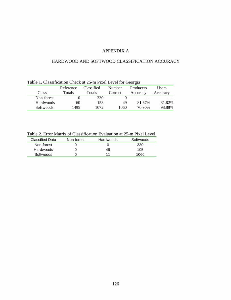
126
APPENDIX A
HARDWOOD AND SOFTWOOD CLASSIFICATION ACCURACY
Table 1. Classification Check at 25-m Pixel Level for Georgia
Class Reference
Totals Classified
Totals Number Correct
Producers Accuracy
Users Accuracy
Non-forest 0 330 0 ----- ----- Hardwoods 60 153 49 81.67% 31.82% Softwoods 1495 1072 1060 70.90% 98.88%
Table 2. Error Matrix of Classification Evaluation at 25-m Pixel Level Classified Data Non-forest Hardwoods Softwoods
Non-forest 0 0 330 Hardwoods 0 49 105 Softwoods 0 11 1060
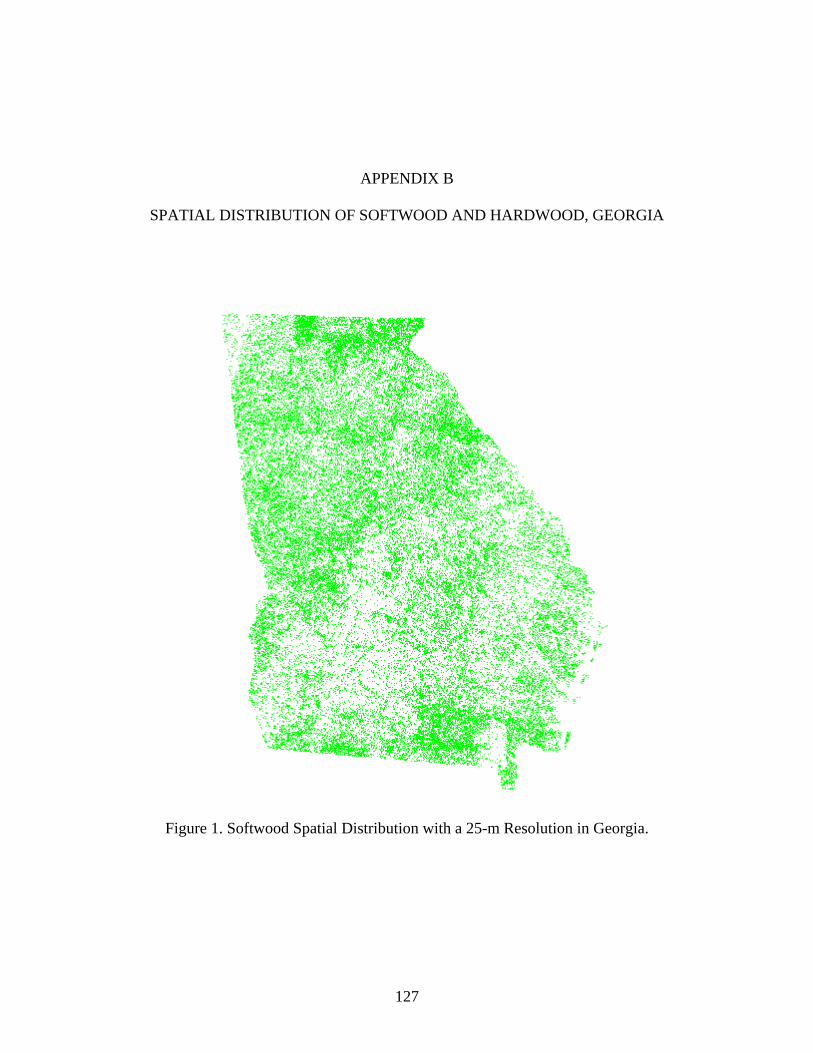
127
APPENDIX B
SPATIAL DISTRIBUTION OF SOFTWOOD AND HARDWOOD, GEORGIA
Figure 1. Softwood Spatial Distribution with a 25-m Resolution in Georgia.
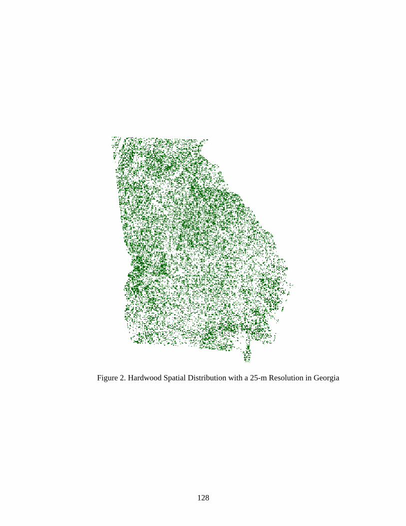
128
Figure 2. Hardwood Spatial Distribution with a 25-m Resolution in Georgia
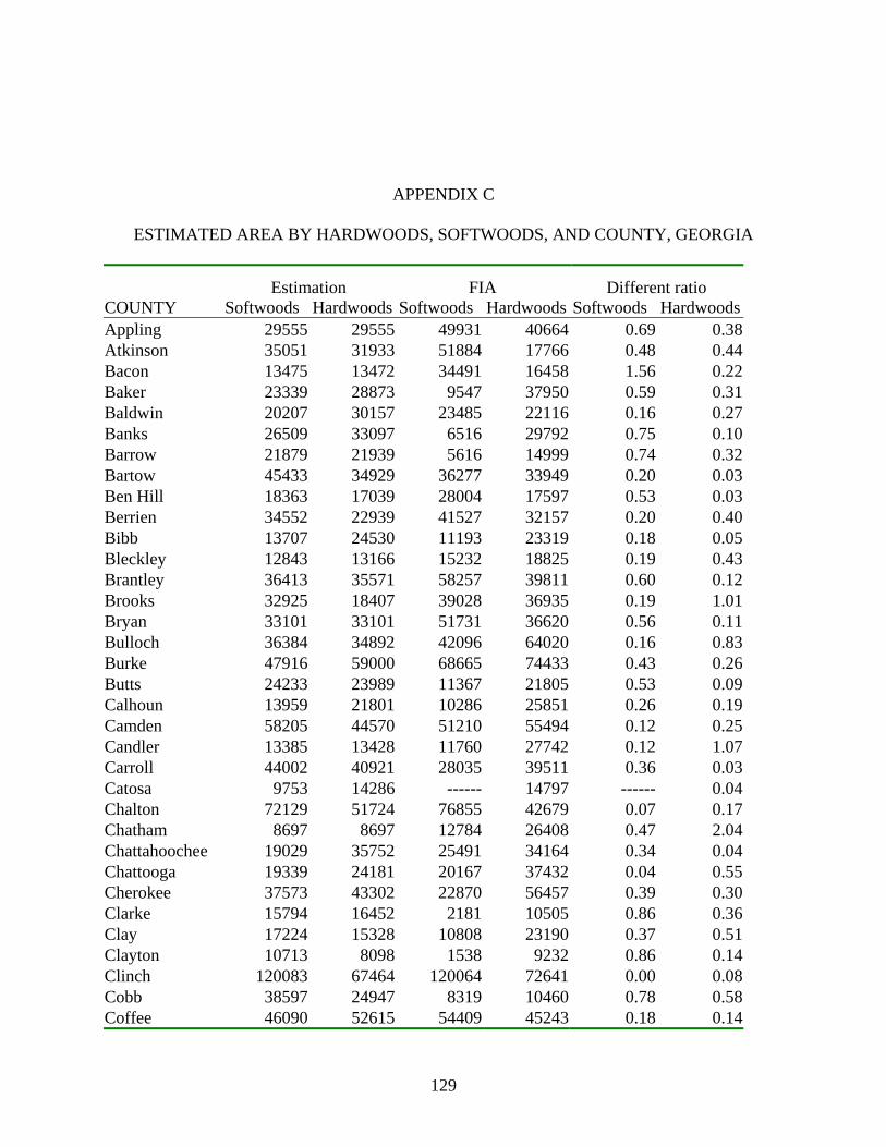
129
APPENDIX C
ESTIMATED AREA BY HARDWOODS, SOFTWOODS, AND COUNTY, GEORGIA
COUNTY Estimation
Softwoods HardwoodsFIA
Softwoods HardwoodsDifferent ratio
Softwoods HardwoodsAppling 29555 29555 49931 40664 0.69 0.38Atkinson 35051 31933 51884 17766 0.48 0.44Bacon 13475 13472 34491 16458 1.56 0.22Baker 23339 28873 9547 37950 0.59 0.31Baldwin 20207 30157 23485 22116 0.16 0.27Banks 26509 33097 6516 29792 0.75 0.10Barrow 21879 21939 5616 14999 0.74 0.32Bartow 45433 34929 36277 33949 0.20 0.03Ben Hill 18363 17039 28004 17597 0.53 0.03Berrien 34552 22939 41527 32157 0.20 0.40Bibb 13707 24530 11193 23319 0.18 0.05Bleckley 12843 13166 15232 18825 0.19 0.43Brantley 36413 35571 58257 39811 0.60 0.12Brooks 32925 18407 39028 36935 0.19 1.01Bryan 33101 33101 51731 36620 0.56 0.11Bulloch 36384 34892 42096 64020 0.16 0.83Burke 47916 59000 68665 74433 0.43 0.26Butts 24233 23989 11367 21805 0.53 0.09Calhoun 13959 21801 10286 25851 0.26 0.19Camden 58205 44570 51210 55494 0.12 0.25Candler 13385 13428 11760 27742 0.12 1.07Carroll 44002 40921 28035 39511 0.36 0.03Catosa 9753 14286 ------ 14797 ------ 0.04Chalton 72129 51724 76855 42679 0.07 0.17Chatham 8697 8697 12784 26408 0.47 2.04Chattahoochee 19029 35752 25491 34164 0.34 0.04Chattooga 19339 24181 20167 37432 0.04 0.55Cherokee 37573 43302 22870 56457 0.39 0.30Clarke 15794 16452 2181 10505 0.86 0.36Clay 17224 15328 10808 23190 0.37 0.51Clayton 10713 8098 1538 9232 0.86 0.14Clinch 120083 67464 120064 72641 0.00 0.08Cobb 38597 24947 8319 10460 0.78 0.58Coffee 46090 52615 54409 45243 0.18 0.14
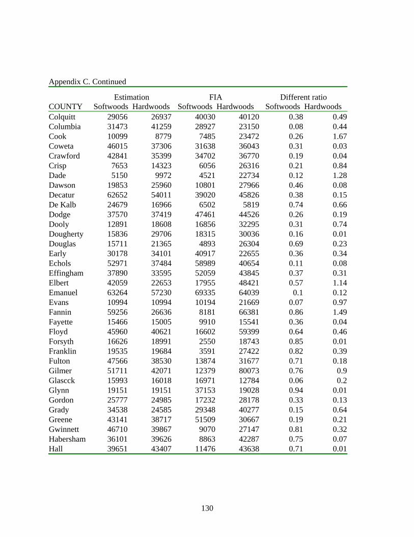
130
Appendix C. Continued
COUNTY Estimation
Softwoods HardwoodsFIA
Softwoods Hardwoods Different ratio
Softwoods Hardwoods Colquitt 29056 26937 40030 40120 0.38 0.49Columbia 31473 41259 28927 23150 0.08 0.44Cook 10099 8779 7485 23472 0.26 1.67Coweta 46015 37306 31638 36043 0.31 0.03Crawford 42841 35399 34702 36770 0.19 0.04Crisp 7653 14323 6056 26316 0.21 0.84Dade 5150 9972 4521 22734 0.12 1.28Dawson 19853 25960 10801 27966 0.46 0.08Decatur 62652 54011 39020 45826 0.38 0.15De Kalb 24679 16966 6502 5819 0.74 0.66Dodge 37570 37419 47461 44526 0.26 0.19Dooly 12891 18608 16856 32295 0.31 0.74Dougherty 15836 29706 18315 30036 0.16 0.01Douglas 15711 21365 4893 26304 0.69 0.23Early 30178 34101 40917 22655 0.36 0.34Echols 52971 37484 58989 40654 0.11 0.08Effingham 37890 33595 52059 43845 0.37 0.31Elbert 42059 22653 17955 48421 0.57 1.14Emanuel 63264 57230 69335 64039 0.1 0.12Evans 10994 10994 10194 21669 0.07 0.97Fannin 59256 26636 8181 66381 0.86 1.49Fayette 15466 15005 9910 15541 0.36 0.04Floyd 45960 40621 16602 59399 0.64 0.46Forsyth 16626 18991 2550 18743 0.85 0.01Franklin 19535 19684 3591 27422 0.82 0.39Fulton 47566 38530 13874 31677 0.71 0.18Gilmer 51711 42071 12379 80073 0.76 0.9Glascck 15993 16018 16971 12784 0.06 0.2Glynn 19151 19151 37153 19028 0.94 0.01Gordon 25777 24985 17232 28178 0.33 0.13Grady 34538 24585 29348 40277 0.15 0.64Greene 43141 38717 51509 30667 0.19 0.21Gwinnett 46710 39867 9070 27147 0.81 0.32Habersham 36101 39626 8863 42287 0.75 0.07Hall 39651 43407 11476 43638 0.71 0.01
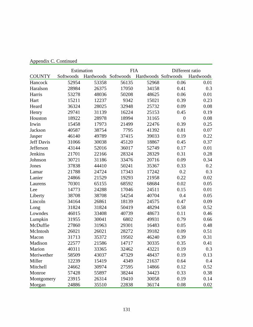
131
Appendix C. Continued
COUNTY Estimation
Softwoods HardwoodsFIA
Softwoods HardwoodsDifferent ratio
Softwoods HardwoodsHancock 52954 53358 56135 52968 0.06 0.01Haralson 28984 26375 17050 34158 0.41 0.3Harris 53278 48036 50208 48625 0.06 0.01Hart 15211 12237 9342 15021 0.39 0.23Heard 36324 28025 32948 25732 0.09 0.08Henry 29741 31139 16224 25153 0.45 0.19Houston 18922 28978 18994 31165 0 0.08Irwin 15458 17973 21499 22476 0.39 0.25Jackson 40587 38754 7795 41392 0.81 0.07Jasper 46140 49789 37415 39033 0.19 0.22Jeff Davis 31066 30038 45120 18867 0.45 0.37Jefferson 43144 52016 36017 52749 0.17 0.01Jenkins 21701 22166 28324 28329 0.31 0.28Johnson 30721 31186 33476 20716 0.09 0.34Jones 37838 44410 50241 35367 0.33 0.2Lamar 21788 24724 17343 17242 0.2 0.3Lanier 24866 21529 19293 21958 0.22 0.02Laurens 70301 65155 68592 68684 0.02 0.05Lee 14773 24288 17046 24511 0.15 0.01Liberty 38708 38708 54254 40704 0.4 0.05Lincoln 34164 26861 18139 24575 0.47 0.09Long 31824 31824 50419 48294 0.58 0.52Lowndes 46015 33408 40739 48673 0.11 0.46Lumpkin 31955 30041 6802 49931 0.79 0.66McDuffie 27860 31963 29301 16483 0.05 0.48McIntosh 26021 26021 28272 39182 0.09 0.51Macon 31713 35372 19502 46240 0.39 0.31Madison 22577 21586 14717 30335 0.35 0.41Marion 40311 33365 32462 43221 0.19 0.3Meriwether 58509 43037 47329 48437 0.19 0.13Miller 12239 15419 4349 21637 0.64 0.4Mitchell 24662 30974 27595 14866 0.12 0.52Monroe 57428 55897 38244 34423 0.33 0.38Montgomery 23915 26314 19410 30058 0.19 0.14Morgan 24886 35510 22838 36174 0.08 0.02
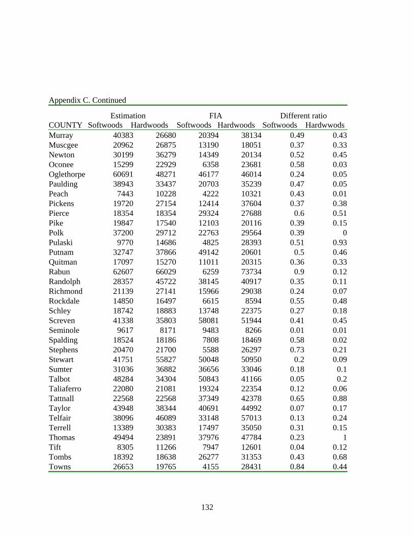
132
Appendix C. Continued
COUNTY Estimation
Softwoods HardwoodsFIA
Softwoods Hardwoods Different ratio
Softwoods HardwwodsMurray 40383 26680 20394 38134 0.49 0.43Muscgee 20962 26875 13190 18051 0.37 0.33Newton 30199 36279 14349 20134 0.52 0.45Oconee 15299 22929 6358 23681 0.58 0.03Oglethorpe 60691 48271 46177 46014 0.24 0.05Paulding 38943 33437 20703 35239 0.47 0.05Peach 7443 10228 4222 10321 0.43 0.01Pickens 19720 27154 12414 37604 0.37 0.38Pierce 18354 18354 29324 27688 0.6 0.51Pike 19847 17540 12103 20116 0.39 0.15Polk 37200 29712 22763 29564 0.39 0Pulaski 9770 14686 4825 28393 0.51 0.93Putnam 32747 37866 49142 20601 0.5 0.46Quitman 17097 15270 11011 20315 0.36 0.33Rabun 62607 66029 6259 73734 0.9 0.12Randolph 28357 45722 38145 40917 0.35 0.11Richmond 21139 27141 15966 29038 0.24 0.07Rockdale 14850 16497 6615 8594 0.55 0.48Schley 18742 18883 13748 22375 0.27 0.18Screven 41338 35803 58081 51944 0.41 0.45Seminole 9617 8171 9483 8266 0.01 0.01Spalding 18524 18186 7808 18469 0.58 0.02Stephens 20470 21700 5588 26297 0.73 0.21Stewart 41751 55827 50048 50950 0.2 0.09Sumter 31036 36882 36656 33046 0.18 0.1Talbot 48284 34304 50843 41166 0.05 0.2Taliaferro 22080 21081 19324 22354 0.12 0.06Tattnall 22568 22568 37349 42378 0.65 0.88Taylor 43948 38344 40691 44992 0.07 0.17Telfair 38096 46089 33148 57013 0.13 0.24Terrell 13389 30383 17497 35050 0.31 0.15Thomas 49494 23891 37976 47784 0.23 1Tift 8305 11266 7947 12601 0.04 0.12Tombs 18392 18638 26277 31353 0.43 0.68Towns 26653 19765 4155 28431 0.84 0.44
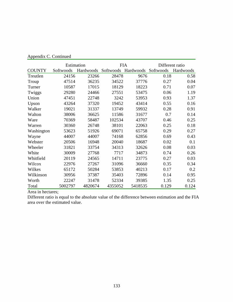
133
Appendix C. Continued
COUNTY Estimation
Softwoods HardwoodsFIA
Softwoods HardwoodsDifferent ratio
Softwoods HardwoodsTreutlen 24156 23266 28478 9676 0.18 0.58Troup 47514 36235 34522 37776 0.27 0.04Turner 10587 17015 18129 18223 0.71 0.07Twiggs 29280 24466 27551 53475 0.06 1.19Union 47451 22748 3242 53953 0.93 1.37Upson 43264 37320 19452 43414 0.55 0.16Walker 19021 31337 13749 59932 0.28 0.91Walton 38006 36625 11586 31677 0.7 0.14Ware 70369 58487 102534 43707 0.46 0.25Warren 30360 26748 38101 22063 0.25 0.18Washington 53623 51926 69071 65758 0.29 0.27Wayne 44007 44007 74168 62856 0.69 0.43Webster 20506 16948 20040 18687 0.02 0.1Wheeler 31821 33754 34313 32626 0.08 0.03White 30009 27768 7717 34873 0.74 0.26Whitfield 20119 24565 14711 23775 0.27 0.03Wilcox 22976 27267 31096 36660 0.35 0.34Wilkes 65172 50284 53853 40213 0.17 0.2Wilkinson 30956 37387 35403 72896 0.14 0.95Worth 22247 31478 52334 39385 1.35 0.25Total 5002797 4820674 4355052 5418535 0.129 0.124Area in hectares; Different ratio is equal to the absolute value of the difference between estimation and the FIA area over the estimated value.
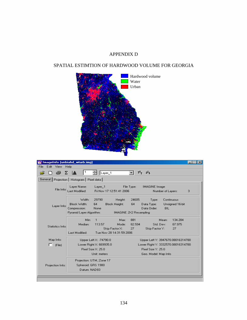
134
APPENDIX D
SPATIAL ESTIMTION OF HARDWOOD VOLUME FOR GEORGIA
Hardwood volume Water Urban
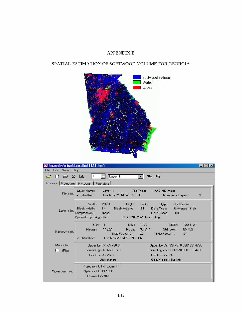
135
APPENDIX E
SPATIAL ESTIMATION OF SOFTWOOD VOLUME FOR GEORGIA
Softwood volume Water Urban