Embed Size (px)
Citation preview
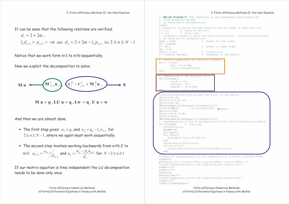
=
==
==
=
∆
−∆+=→∆
=
∆+
∆
∆ =
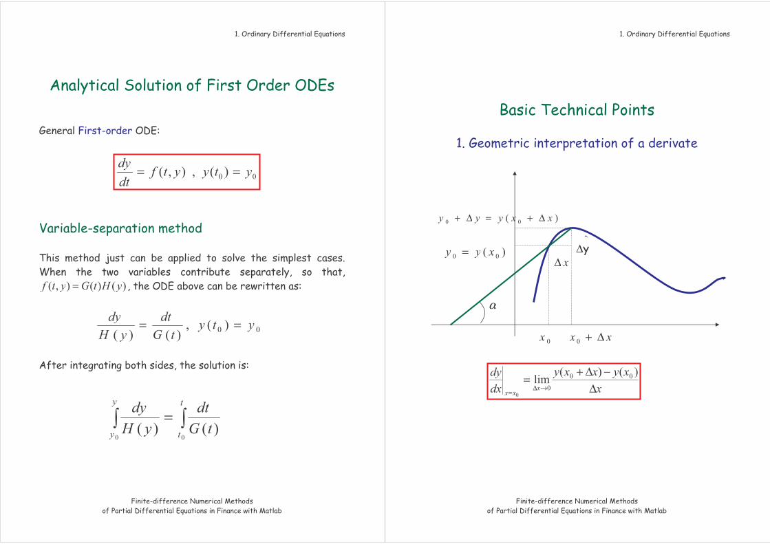
α
∆+=∆+
∆
- - -
-
-
-
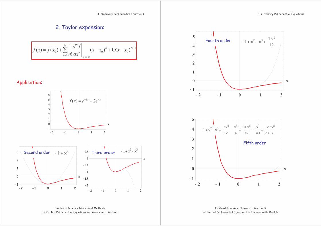
-1+x2- x3
+
==−Ο+−+=
- - -
−− −=
− − −
- 1+ x2
- - -
- 1 + x2 - x3+7x4
12
- - -
-1+x2- x3+7x4
12-x5
4+31x6
360-x7
40+127x8
20160
∆+=∆+≈∆+
∆Ο+∆+=+ ∆+=
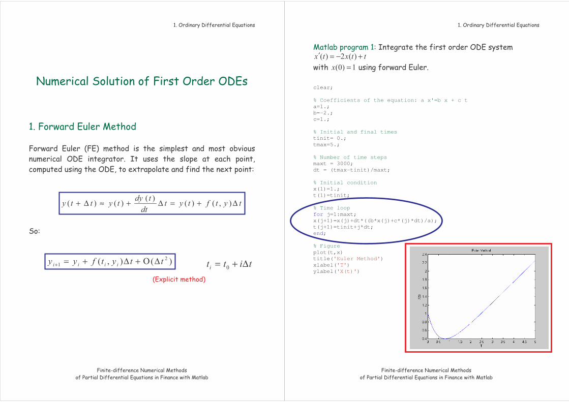
+−=′ = clear; % Coefficients of the equation: a x'=b x + c t a=1.; b=-2.; c=1.; % Initial and final times tinit= 0.; tmax=5.; % Number of time steps maxt = 3000; dt = (tmax-tinit)/maxt; % Initial condition x(1)=1.; t(1)=tinit; % Time loop for j=1:maxt; x(j+1)=x(j)+dt*((b*x(j)+c*(j)*dt)/a); t(j+1)=tinit+j*dt; end; % Figure plot(t,x) title('Euler Method') xlabel('T') ylabel('X(t)')
∆
∆Ο+∆+= −+
∆−=−
∆Ο+∆+= +++
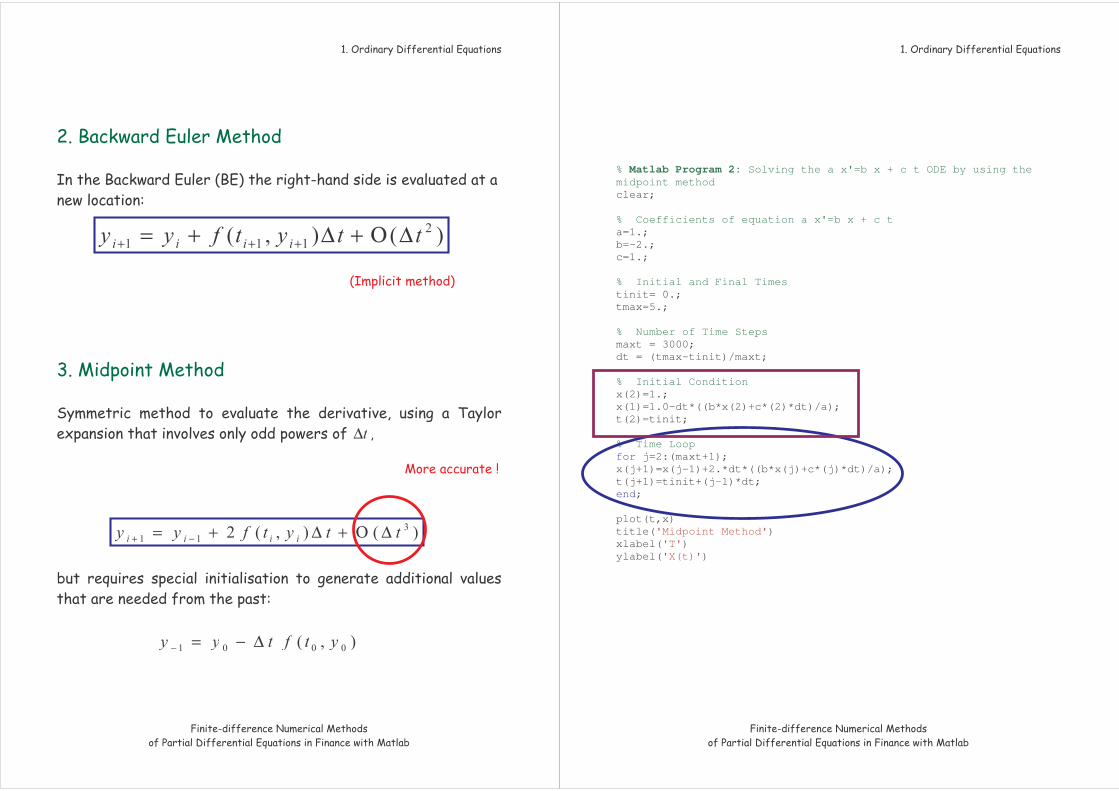
% Matlab Program 2: Solving the a x'=b x + c t ODE by using the midpoint method clear; % Coefficients of equation a x'=b x + c t a=1.; b=-2.; c=1.; % Initial and Final Times tinit= 0.; tmax=5.; % Number of Time Steps maxt = 3000; dt = (tmax-tinit)/maxt; % Initial Condition x(2)=1.; x(1)=1.0-dt*((b*x(2)+c*(2)*dt)/a); t(2)=tinit; % Time Loop for j=2:(maxt+1); x(j+1)=x(j-1)+2.*dt*((b*x(j)+c*(j)*dt)/a); t(j+1)=tinit+(j-1)*dt; end; plot(t,x) title('Midpoint Method') xlabel('T') ylabel('X(t)')
∆∆+∆++=+
∆Ο++=
+∆+∆=
∆=
+
• • •
∆Ο+++++=
+∆+∆=
+∆+∆=
+∆+∆=
∆=
+
=+′+′′ =++
• ≠ ++=
• ℜ∈== ++=
′=′==+′+′′
=+′+′′ =′=
−−=′
=′
′==
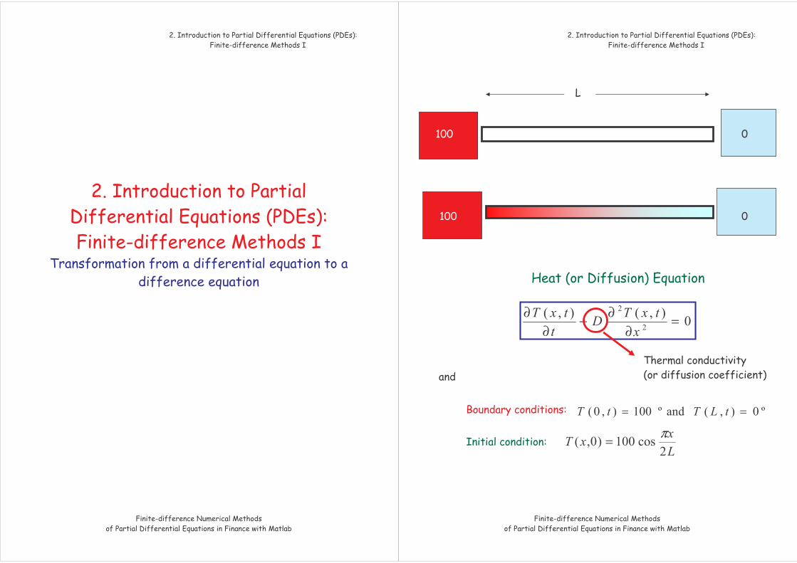
=∂
∂−∂
∂
==
π=
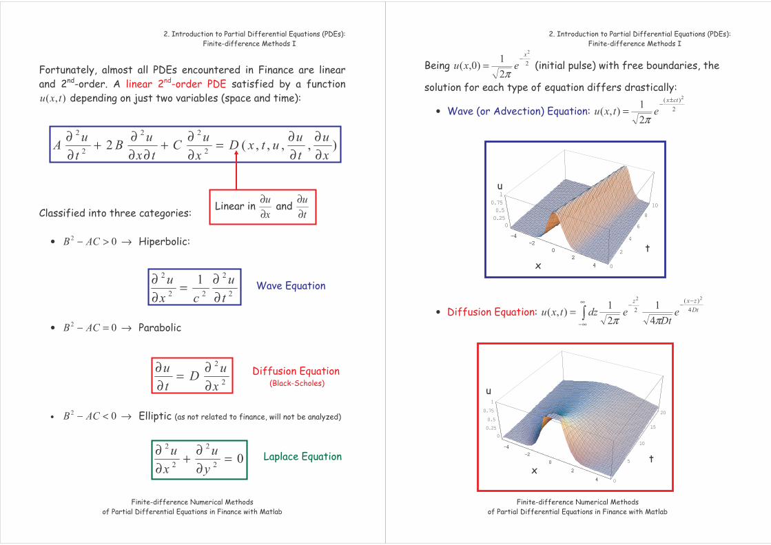
• →>−
• →=−
• →<−
∂∂
∂∂=
∂∂+
∂∂∂+
∂∂
∂∂
∂∂
∂∂=
∂∂
∂∂=
∂∂
=∂∂+
∂∂
−
=π
•
±−
=π
•
−−−∞
∞−=
ππ
-4-2
02
4 0
2
4
6
8
10
00.250.5
0.75
1
-4-2
02
4
-4
-2
0
2
4 0
5
10
15
20
0
0.25
0.5
0.75
1
-4
-2
0
2
4
•
•
•
==
∀Ω∂∈∀=
∂∂+
τλτλ τ λ βα ττ = τ > = =τ →∞→ τ
>∂∂=
∂∂ ττ
τ τξ = ξτ =
=+ξ
ξξ
=∞=
+= −ξ
ξ
∞
−=ξπ
ξ
∞
−=τπ
τ
δ= →±∞→ τ τ τξ =
ξττ δδ −=
=+ξξ
ξδδ
−τ ∞
∞− τ
τ
+= − ξδ ξ
>∂∂=
∂∂ ττ
π= =∞
∞− τδ
τ
δ πττ
−=
∞<<∞− >τ =
ξξδξ −= ∞
∞−
τδ πτ
τ
−−=−
−δ
τ
πττ
−−
∞
∞−=
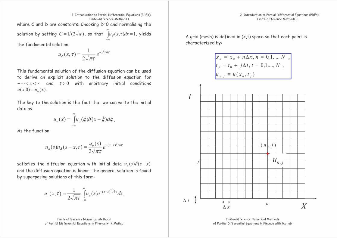
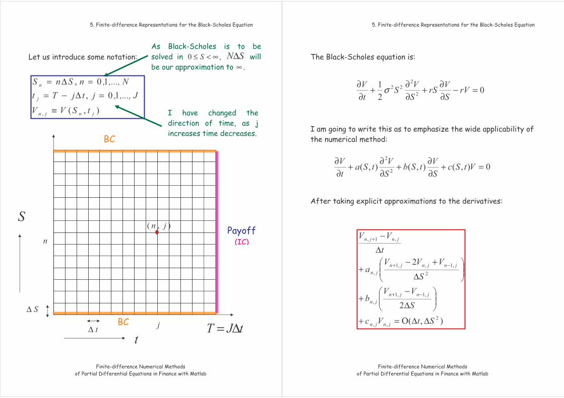
≡=∆+=
=∆+=
∆∆
∂∂=
∂∂
∆Ο+
∆−
=∂∂ +
∆Ο+
∆−
=∂∂ −+
+ + +
∆−
−=∆− −++
( ) −++ −
∆∆−=

% Matlab Program 3: Square-wave Test for the Explicit Method to solve % the Advection Equation clear; % Parameters to define the advection equation and the range in space and % time Lmax = 1.0; % Maximum length Tmax = 1.; % Maximum time c = 1.0; % Advection velocity % Parameters needed to solve the equation within the explicit method maxt = 3000; % Number of time steps dt = Tmax/maxt; n = 30; % Number of space steps nint=15; % The wave-front: intermediate point from which u=0 dx = Lmax/n; b = c*dt/(2.*dx); % Initial value of the function u (amplitude of the wave) for i = 1:(n+1) if i < nint u(i,1)=1.; else u(i,1)=0.; end x(i) =(i-1)*dx; end % Value of the amplitude at the boundary for k=1:maxt+1 u(1,k) = 1.; u(n+1,k) = 0.; time(k) = (k-1)*dt; end % Implementation of the explicit method for k=1:maxt % Time loop for i=2:n % Space loop u(i,k+1) =u(i,k)-b*(u(i+1,k)-u(i-1,k)); end end % Graphical representation of the wave at different selected times plot(x,u(:,1),'-',x,u(:,10),'-',x,u(:,50),'-',x,u(:,100),'-') title('Square-wave test within the Explicit Method I') xlabel('X') ylabel('Amplitude(X)')
∆=
ξ
∆= ξ >ξ
∆
∆∆−= ξ >ξ
∆ ∆
=∂∂
=
=− −=
λ=
∆= λ
<ξ
( )
−+ +→
( ) ( )
−+−++ −
∆∆−+=
∆
∆∆−∆= ξ
≤∆∆
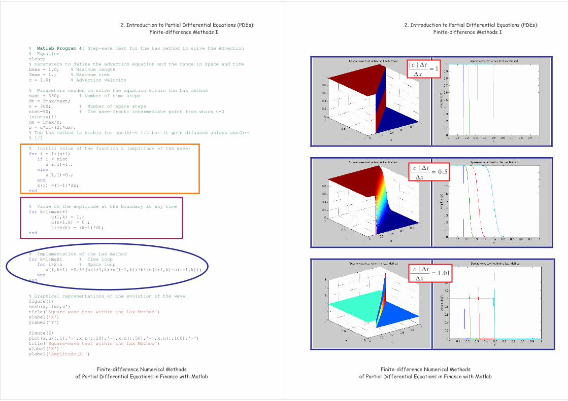
% Matlab Program 4: Step-wave Test for the Lax method to solve the Advection % Equation clear; % Parameters to define the advection equation and the range in space and time Lmax = 1.0; % Maximum length Tmax = 1.; % Maximum time c = 1.0; % Advection velocity % Parameters needed to solve the equation within the Lax method maxt = 350; % Number of time steps dt = Tmax/maxt; n = 300; % Number of space steps nint=50; % The wave-front: intermediate point from which u=0 (nint<n)!! dx = Lmax/n; b = c*dt/(2.*dx); % The Lax method is stable for abs(b)=< 1/2 but it gets difussed unless abs(b)= % 1/2 % Initial value of the function u (amplitude of the wave) for i = 1:(n+1) if i < nint u(i,1)=1.; else u(i,1)=0.; end x(i) =(i-1)*dx; end % Value of the amplitude at the boundary at any time for k=1:maxt+1 u(1,k) = 1.; u(n+1,k) = 0.; time(k) = (k-1)*dt; end % Implementation of the Lax method for k=1:maxt % Time loop for i=2:n % Space loop u(i,k+1) =0.5*(u(i+1,k)+u(i-1,k))-b*(u(i+1,k)-u(i-1,k)); end end % Graphical representations of the evolution of the wave figure(1) mesh(x,time,u') title('Square-wave test within the Lax Method') xlabel('X') ylabel('T') figure(2) plot(x,u(:,1),'-',x,u(:,20),'-',x,u(:,50),'-',x,u(:,100),'-') title('Square-wave test within the Lax Method') xlabel('X') ylabel('Amplitude(X)')
=∆∆
=∆∆
=∆∆
• →>∆∆
• →<∆∆
• →=∆∆
∂∂
∆∆+
∂∂=
∂∂
ξ
∆
∆∆=− ξξ
∆∆∆−±∆
∆∆=
ξ
=ξ ∆≤∆
∆−
=∆− −+−+
∂∂
∂∂=
∂∂
∆Ο+
∆−
=∂∂ +
∆Ο+
∆+−
=∂∂ −+
∂∂=
∂∂
∆∆=α
∆+−
=∆− −++
−++ +−+= ααα
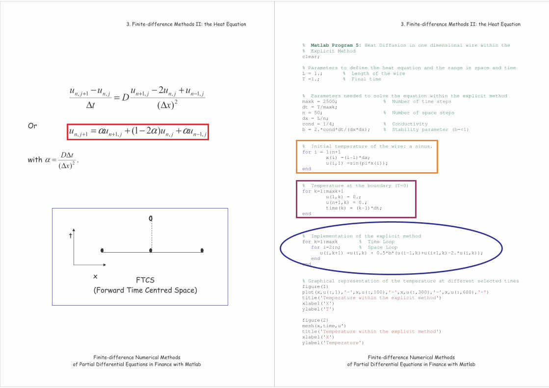
% Matlab Program 5: Heat Diffusion in one dimensional wire within the % Explicit Method clear; % Parameters to define the heat equation and the range in space and time L = 1.; % Length of the wire T =1.; % Final time % Parameters needed to solve the equation within the explicit method maxk = 2500; % Number of time steps dt = T/maxk; n = 50; % Number of space steps dx = L/n; cond = 1/4; % Conductivity b = 2.*cond*dt/(dx*dx); % Stability parameter (b=<1) % Initial temperature of the wire: a sinus. for i = 1:n+1 x(i) =(i-1)*dx; u(i,1) =sin(pi*x(i)); end % Temperature at the boundary (T=0) for k=1:maxk+1 u(1,k) = 0.; u(n+1,k) = 0.; time(k) = (k-1)*dt; end % Implementation of the explicit method for k=1:maxk % Time Loop for i=2:n; % Space Loop u(i,k+1) =u(i,k) + 0.5*b*(u(i-1,k)+u(i+1,k)-2.*u(i,k)); end end % Graphical representation of the temperature at different selected times figure(1) plot(x,u(:,1),'-',x,u(:,100),'-',x,u(:,300),'-',x,u(:,600),'-') title('Temperature within the explicit method') xlabel('X') ylabel('T') figure(2) mesh(x,time,u') title('Temperature within the explicit method') xlabel('X') ylabel('Temperature')
=
∆∆
=
∆∆
∆= ξ
( )
∆
∆∆−=
ξ ≤ξ
<<∆ <<∆
≤
∆∆
∆

∆+−
=∆− +−++++
+
∆+
=
α
ξ
≤ξ ∆ ∆
∞→∆
∆∆=−=
−++−= ++++−
α
ααα
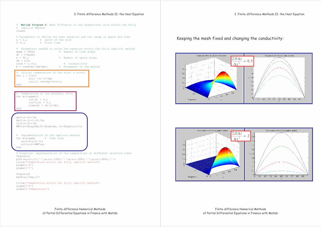
% Matlab Program 6: Heat Diffusion in one dimensional wire within the Fully % Implicit Method clear; % Parameters to define the heat equation and the range in space and time L = 1.; % Lenth of the wire T =1.; % Final time % Parameters needed to solve the equation within the fully implicit method maxk = 2500; % Number of time steps dt = T/maxk; n = 50.; % Number of space steps dx = L/n; cond = 1./4.; % Conductivity b = cond*dt/(dx*dx); % Parameter of the method % Initial temperature of the wire: a sinus. for i = 1:n+1 x(i) =(i-1)*dx; u(i,1) =sin(pi*x(i)); end % Temperature at the boundary (T=0) for k=1:maxk+1 u(1,k) = 0.; u(n+1,k) = 0.; time(k) = (k-1)*dt; end aa(1:n-2)=-b; bb(1:n-1)=1.+2.*b; cc(1:n-2)=-b; MM=inv(diag(bb,0)+diag(aa,-1)+diag(cc,1)); % Implementation of the implicit method for k=2:maxk % Time Loop uu=u(2:n,k-1); u(2:n,k)=MM*uu; end % Graphical representation of the temperature at different selected times figure(1) plot(x,u(:,1),'-',x,u(:,100),'-',x,u(:,300),'-',x,u(:,600),'-') title('Temperature within the fully implicit method') xlabel('X') ylabel('T') figure(2) mesh(x,time,u') title('Temperature within the fully implicit method') xlabel('X') ylabel('Temperature')
=
∆∆
=
∆∆
∆
+−++−=
∆− −++−++++
∆+
∆−
=
α
αξ
≤ξ ∆
−≤≤
++++−+− −++−=+−+ αααααα
−−
−−
=
−+−−+
−+−−+−
−
+
+−
+
+
ααααα
αααααα
ααααα
αααααα
+
+ +
+=+ +++
−+−−+
−+−−+−
+
+−
+
+
ααααα
αααααα
+
+
+++
+
+
+−
+
+=
−
−
+
+−−+−
−+−−+
α
α
ααααα
ααα
αα
+−= +++
+−Μ= +
−++
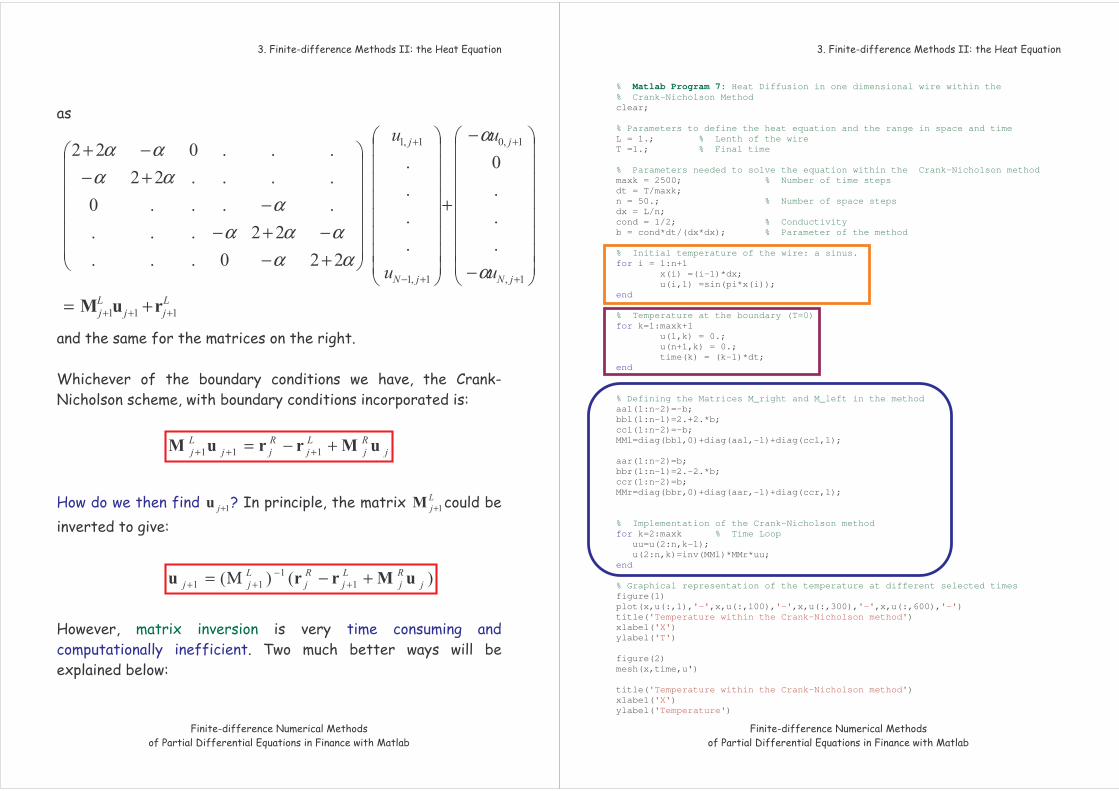
% Matlab Program 7: Heat Diffusion in one dimensional wire within the % Crank-Nicholson Method clear; % Parameters to define the heat equation and the range in space and time L = 1.; % Lenth of the wire T =1.; % Final time % Parameters needed to solve the equation within the Crank-Nicholson method maxk = 2500; % Number of time steps dt = T/maxk; n = 50.; % Number of space steps dx = L/n; cond = 1/2; % Conductivity b = cond*dt/(dx*dx); % Parameter of the method % Initial temperature of the wire: a sinus. for i = 1:n+1 x(i) =(i-1)*dx; u(i,1) =sin(pi*x(i)); end % Temperature at the boundary (T=0) for k=1:maxk+1 u(1,k) = 0.; u(n+1,k) = 0.; time(k) = (k-1)*dt; end % Defining the Matrices M_right and M_left in the method aal(1:n-2)=-b; bbl(1:n-1)=2.+2.*b; ccl(1:n-2)=-b; MMl=diag(bbl,0)+diag(aal,-1)+diag(ccl,1); aar(1:n-2)=b; bbr(1:n-1)=2.-2.*b; ccr(1:n-2)=b; MMr=diag(bbr,0)+diag(aar,-1)+diag(ccr,1); % Implementation of the Crank-Nicholson method for k=2:maxk % Time Loop uu=u(2:n,k-1); u(2:n,k)=inv(MMl)*MMr*uu; end % Graphical representation of the temperature at different selected times figure(1) plot(x,u(:,1),'-',x,u(:,100),'-',x,u(:,300),'-',x,u(:,600),'-') title('Temperature within the Crank-Nicholson method') xlabel('X') ylabel('T') figure(2) mesh(x,time,u') title('Temperature within the Crank-Nicholson method') xlabel('X') ylabel('Temperature')
=
∆∆
=
∆∆
[L,U]=lu(M))
+ =
=
+−−+−
−+−−+
−
−−
−
−
−
ααααα
ααα
αα
• = −−= −≤≤
•
−
−− =
+−= ≥≥−
−≤≤−+=−==+=
−−−
ααα
+−= +++
====
% Matlab Program 8: Heat Diffusion in one dimensional wire within the % Crank-Nicholson Method % by using the LU decomposition. clear; % Parameters to define the heat equation and the range in space and time L = 1.; % Lenth of the wire T = 1.; % Final time % Parameters needed to solve the equation within the Crank-Nicholson method % by using the LU decomposition maxk = 2500; % Number of time steps dt = T/maxk; n = 50.; % Number of space steps dx = L/n; cond = 1./4.; % Conductivity b = cond*dt/(dx*dx); % Parameter of the method % Initial temperature of the wire: a sinus. for i = 1:n+1 x(i) =(i-1)*dx; v(i,1) =sin(pi*x(i)); end % Temperature at the boundary (T=0) for k=1:maxk+1 v(1,k) = 0.; v(n+1,k) = 0.; time(k) = (k-1)*dt; end % Defining the Matrices M_right and M_left in the method aal(1:n-2)=-b; bbl(1:n-1)=2.+2.*b; ccl(1:n-2)=-b; MMl=diag(bbl,0)+diag(aal,-1)+diag(ccl,1); [L,U]=lu(MMl); % LU decomposition aar(1:n-2)=b; bbr(1:n-1)=2.-2.*b; ccr(1:n-2)=b; MMr=diag(bbr,0)+diag(aar,-1)+diag(ccr,1); % Implementation of the LU decomposition within the Crank-Nicholson method for k=2:maxk % Time Loop vv=v(2:n,k-1); qq=MMr*vv; w(1)=qq(1); for j=2:n-1 w(j)=qq(j)-L(j,j-1)*w(j-1); end v(n,k)=w(n-1)/U(n-1,n-1); for i=n-1:-1:2 v(i,k)=(w(i-1)-U(i-1,i)*v(i+1,k))/U(i-1,i-1); end end % Graphical representation of the temperature at different selected times figure(1) plot(x,v(:,1),'-',x,v(:,100),'-',x,v(:,300),'-',x,v(:,600),'-') title('Temperature within the Crank-Nicholson method (LU)') xlabel('X') ylabel('T') figure(2) mesh(x,time,v') title('Temperature within the Crank-Nicholson method (LU)') xlabel('X') ylabel('Temperature')
=
=+++
=+++=+++
++−=
++−=++−=
++=
+
[ ][ ]
[ ]
++−=
++−=
++−=
+
+
+
[ ] +−= −+
−−= =
−
=
++
−+
ω −= ω ω
−−+−= =
−
=
++
ωω
( )[ ] −−−−+ +−−+= ωωωω
( )[ ] −−−+ −−+= ωωω

≡µσ Π ∆
∆−=Π
σµ +=
∆−=Π
∂∂+
∂∂+
∂∂=
σ
∆−
∂∂+
∂∂+
∂∂=Π
σ
∂∂=∆
∆
∆−
∂∂+
∂∂+
∂∂=Π
σ
∂∂+
∂∂=Π
σ
Π=Π
=−
∂∂+
∂∂+
∂∂
σ
σ
σ
σ
•
•
•
•
•
•
= ∞→ = =
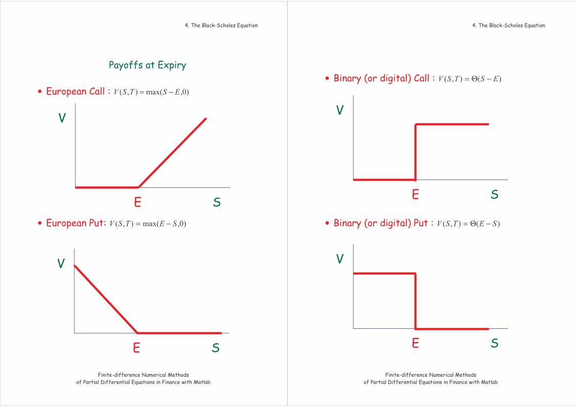
• −=
• −=
• −Θ=
• −Θ=
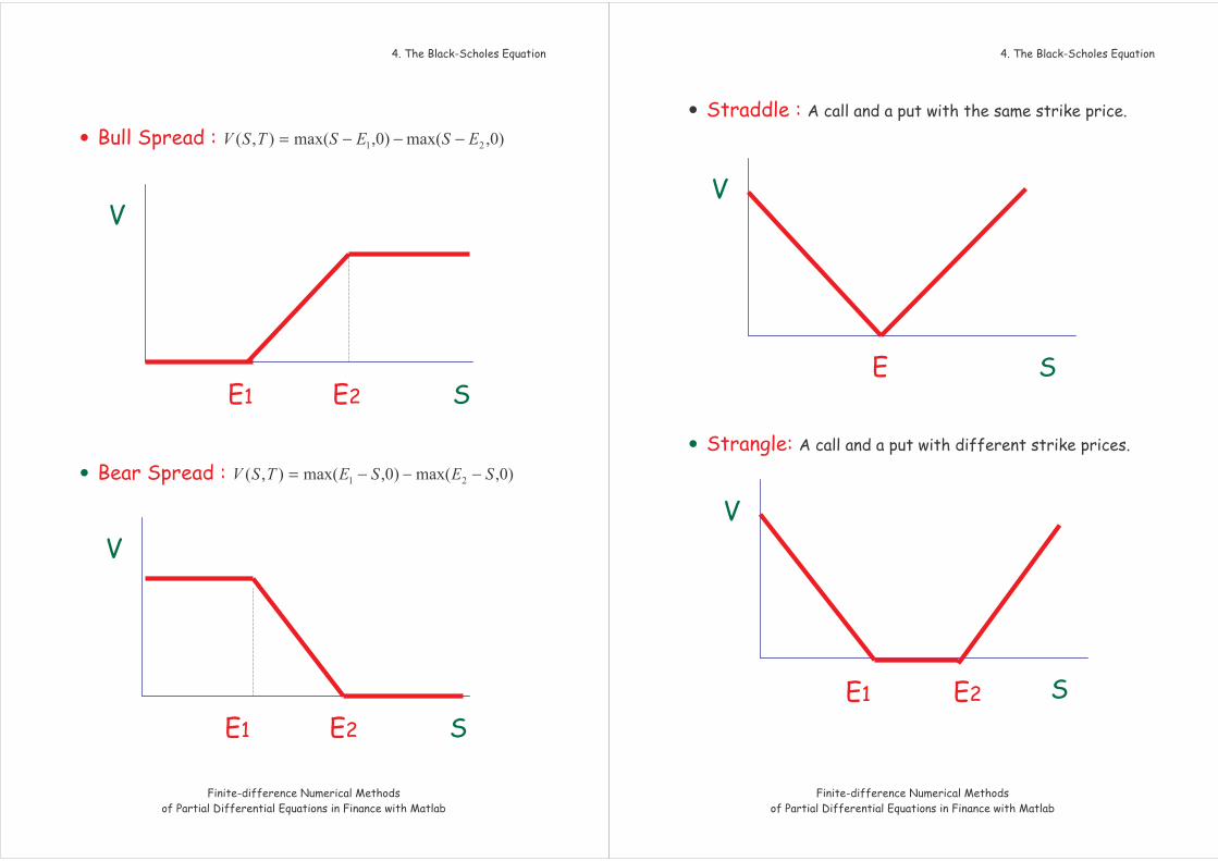
• −−−=
• −−−=
•
•
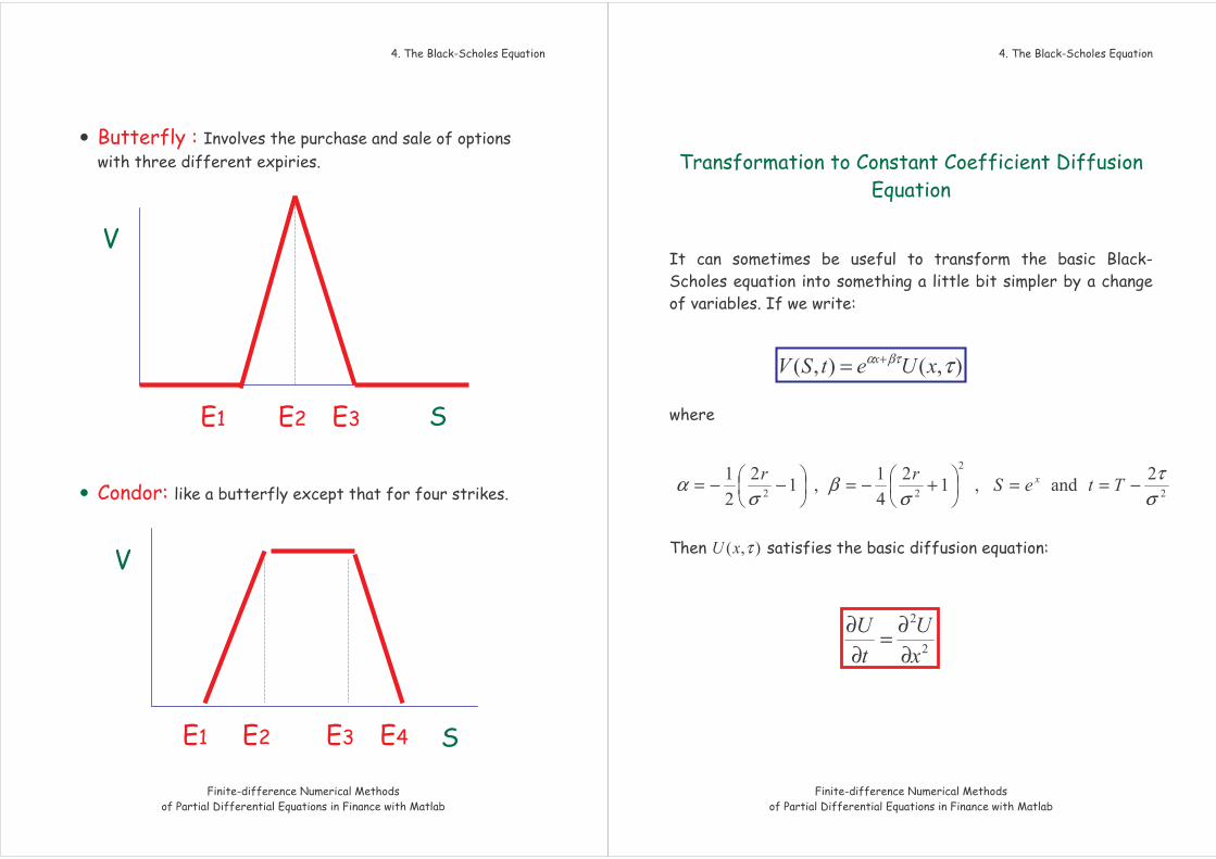
•
•
τ
τβτα +=
στ
σβ
σα −==
+−=
−−=
∂∂=
∂∂
−−= −=τ =ξ
=−
∂∂+
∂∂+
∂∂
σ
=
∂∂+
∂∂+
∂∂
σ
∂∂+
∂∂=
∂∂
σ
τ
ξσ
ξσ
τ ∂∂−+
∂∂=
∂∂
τσξ −+=
τ =
→τ
′−δ
= =
∂∂=
∂∂ στ
τσ
σπττ
′−
−= ′
=′′∞
∞−
′−−
→τσ
τ σπτ
>τ
•
−−−=
−
−++=
σ
σ
−
−−+=
σ
σ
∞−
−=
π
•
−+−−= −−
∞
∞−
′′−−
′=
τσ
σπττ
∞
−−−+′−−−
′′′
−=
σ
σ
σπ
• ∂∂=∆
∆ ∆
•
∂∂=Γ Γ ∆
Γ
• ∂∂=Θ
∆
• σ∂∂=
• ∂∂=ρ
=−
∂∂−+
∂∂+
∂∂
σ
=−
∂∂−+
∂∂+
∂∂
σ
=−
∂∂++
∂∂+
∂∂
σ
−=
=
=−∂∂+
∂∂
σ
[ ]
=−
∂∂−+
∂∂+
∂∂
σ
α α =
=−
∂∂
+−+
∂∂+
∂∂
ασασα
+=
=−
∂∂−+
∂∂+
∂∂+
∂∂+
∂∂
λσ
≡=∆−=
=∆=
∞<≤ ∆ ∞
∆
∆
∆=
=−
∂∂+
∂∂+
∂∂
σ
=+∂∂+
∂∂+
∂∂
∆∆Ο=+
∆−
+
∆+−
+
∆−
−+
−+
+
∆∆=ν
∆∆=ν
Ο+
++
∆+−+
−=
+
−+
νν
ν
νν
[ ]
Ο+
∆++
∆+−+
∆=
+
−+
σ
σ
σ
−= − + − + ∀=
−−−
∆−−∆=
−−=
∆−= =
−∆−= −− −=
=−∂∂
∞→→∂∂
−
=+ −+=
∆∆∆Ο ∆∆∆Ο −∆Ο= ∆∆Ο
∆= ξ
( )[ ]
∆+−∆+∆+=
ννξ
<ξ ∆
•
• ν
<ν
•
( )
νν
ν
≤
≤∆−≤
σ=∆≤∆
( )
σ=≤∆
∆Ο ∆Ο
•
•
∆−
=∂∂≤
∆−
=∂∂≥
−−
++
∆Ο+
∆∆+−∆++−=
∂∂
∆Ο+
∆∆−+∆−−=
∂∂
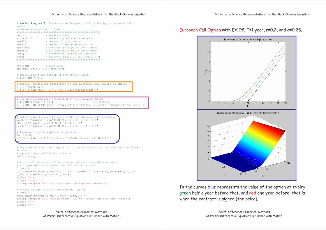
% Matlab Program 9: Evaluates an European Call option by using an explicit method % Parameters of the problem: %%%%%%%%%%%%%%%%%%%%%%%%%%%%%%%%%%%%%%%%%%%%%%%%%%%% r=0.2; % Interest rate sigma=0.25; % Volatility of the underlying M=1600; % Number of time points N=160; % Number of share price points Smax=20; % Maximum share price considered Smin=0; % Minimum share price considered T=1.; % Maturation (expiry)of contract E=10; % Exercise price of the underlying %%%%%%%%%%%%%%%%%%%%%%%%%%%%%%%%%%%%%%%%%%%%%%%%%%%% dt=(T/M); % Time step ds=(Smax-Smin)/N; % Price step % Initializing the matrix of the option value v(1:N,1:M) = 0.0; % Initial conditions prescribed by the European Call payoff at expiry: V(S,T)=max(S-E,0) v(1:N,1)=max((Smin+(0:N-1)*ds-E),zeros(size(1:N)))'; % Boundary conditions prescribed by the European Call: v(1,2:M)=zeros(M-1,1)'; % V(0,t)=0 v(N,2:M)=((N-1)*ds+Smin)-E*exp(-r*(1:M-1)*dt); % V(S,t)=S-Eexp[-r(T-t)] as S -> infininty. % Determining the matrix coeficients of the explicit algorithm aa=0.5*dt*(sigma*sigma*(1:N-2).*(1:N-2)-r*(1:N-2))'; bb=1-dt*(sigma*sigma*(1:N-2).*(1:N-2)+r)'; cc=0.5*dt*(sigma*sigma*(1:N-2).*(1:N-2)+r*(1:N-2))'; % Implementing the explicit algorithm for i=2:M, v(2:N-1,i)=bb.*v(2:N-1,i-1)+cc.*v(3:N,i-1)+aa.*v(1:N-2,i-1); end % Reversal of the time components in the matrix as the solution of the Black-Scholes % equation was performed backwards v=fliplr(v); % Figure of the value of the option, V(S,t), as a function of S % at three different times:t=0, T/2 and T (expiry). figure(1) plot(Smin+ds*(0:N-1),v(1:N,1)','r-',Smin+ds*(0:N-1),v(1:N,round(M/2))','g-',Smin+ds*(0:N-1),v(1:N,M)','b-'); xlabel('S'); ylabel('V(S,t)'); title('European Call Option within the Explicit Method'); % Figure of the Value of the option, V(S,t) figure(2) mesh(Smin+ds*(0:N-1),dt*(0:M-1),v(1:N,1:M)') title('European Call Option value, V(S,t), within the Explicit Method') xlabel('S') ylabel('t')
σ
∆∆Ο=+
∆−
+
∆+−
+
∆−
++
+−+++
+−++++
+
∆∆=ν
∆∆=ν
−= − + − +
Ο+
+−+
∆−++
−−=
++++
+++
+−++
νν
ν
νν
∆∆Ο=++
∆−
+
∆−
+
∆+−
+
∆+−
+
∆−
++
−+
+−+++
−+
+−++++
+
−≤≤
+−
++++++−+
−−+−=+++
νν
ν
νν
−=
∆+−=
+=
+
−−−−−
−−−−−−
=
++
++
−−−−
−−
+
+−
+
+
+−+−+−
+−+−
+++
+++
+=+ +++
+ + =
−−−= =+
∆+−+ −∆=
++
++
+
+−
+
+
+−+−+−
+−+−
+++
+++
+++
++−
++
+−
+
+−+−
+−+−
++
++
+=
+
++
++
=∂∂
=
+−= +++
+−+−++++ −=−=
++−+
+−++
+−
+
+−+−+−+−
+−+−
++
++++
+
=
+−Μ= +
−++
=
++
++
−
−−
−
−
−
−−
−−−
−
• = −−= −≤≤
•
−
−− =
+−= ≥≥−
−≤≤−+===+=
−−−−
+−= +++
====
++=
[ ][ ]
[ ]
++−=
++−=
++−=
+
+
+
[ ] +−= −+
−+
−−= =
−
=
++
−−+−= =
−
=
++
ωω
( )[ ] −−−−+ +−−+= ωωωω
• ∆ ∆
•
•
•
∆∆Ο
∂∂=
∂∂
∆+−
=∆− −++
∆+−
=∆− +−++++
θ
=θ
θ
=θ
∆
∆−=
θ
∆
+−+
∆
+−−=
∆− +−+++−++
θθ
∆∆∆−∆−∆Ο
θ
∆∆∆∆
∆+−
=∆− −+−+
∆+−−
=∆− −−++−+
−−++ −++=+ ννν
∆∆Ο ( )
+∆+∆+∆+=
εεε
++∆
∆+
=
=
=+∆+∆+∆+
εε
εεε
( )
++∆
∆+
=
=
=+∆+∆+∆+
εε
εεε
∆∆=
∆∆
∆−∆∆−∆
=
≥
( ) +−+ +++=
+
∆
−−+−= =
−
=
++
ωω
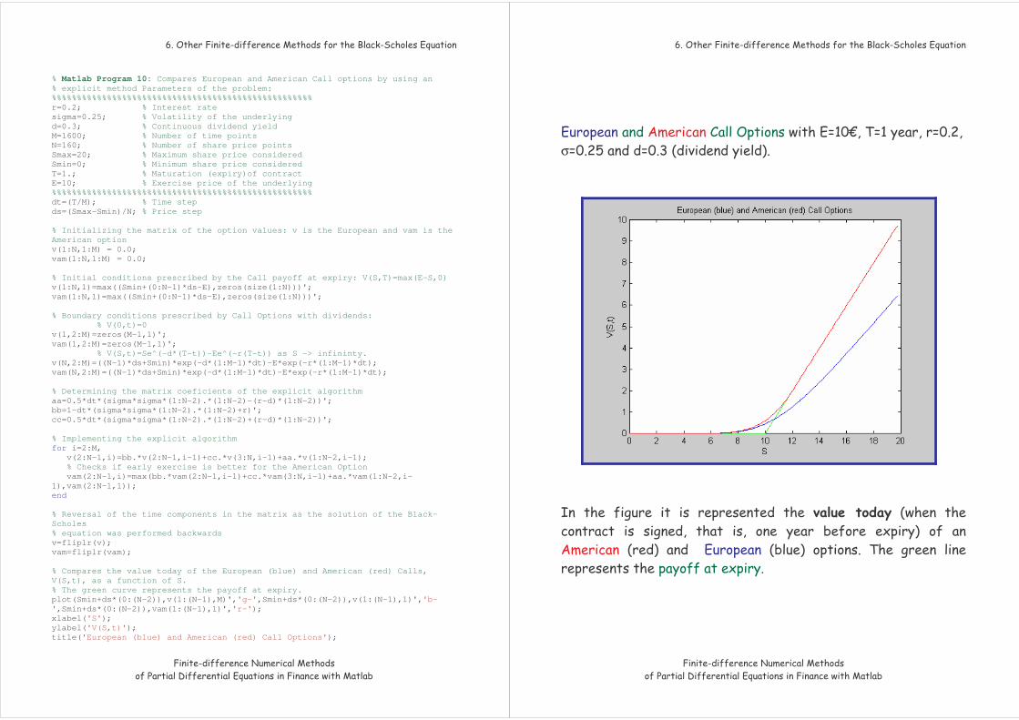
% Matlab Program 10: Compares European and American Call options by using an % explicit method Parameters of the problem: %%%%%%%%%%%%%%%%%%%%%%%%%%%%%%%%%%%%%%%%%%%%%%%%%%%% r=0.2; % Interest rate sigma=0.25; % Volatility of the underlying d=0.3; % Continuous dividend yield M=1600; % Number of time points N=160; % Number of share price points Smax=20; % Maximum share price considered Smin=0; % Minimum share price considered T=1.; % Maturation (expiry)of contract E=10; % Exercise price of the underlying %%%%%%%%%%%%%%%%%%%%%%%%%%%%%%%%%%%%%%%%%%%%%%%%%%%% dt=(T/M); % Time step ds=(Smax-Smin)/N; % Price step % Initializing the matrix of the option values: v is the European and vam is the American option v(1:N,1:M) = 0.0; vam(1:N,1:M) = 0.0; % Initial conditions prescribed by the Call payoff at expiry: V(S,T)=max(E-S,0) v(1:N,1)=max((Smin+(0:N-1)*ds-E),zeros(size(1:N)))'; vam(1:N,1)=max((Smin+(0:N-1)*ds-E),zeros(size(1:N)))'; % Boundary conditions prescribed by Call Options with dividends: % V(0,t)=0 v(1,2:M)=zeros(M-1,1)'; vam(1,2:M)=zeros(M-1,1)'; % V(S,t)=Se^(-d*(T-t))-Ee^(-r(T-t)) as S -> infininty. v(N,2:M)=((N-1)*ds+Smin)*exp(-d*(1:M-1)*dt)-E*exp(-r*(1:M-1)*dt); vam(N,2:M)=((N-1)*ds+Smin)*exp(-d*(1:M-1)*dt)-E*exp(-r*(1:M-1)*dt); % Determining the matrix coeficients of the explicit algorithm aa=0.5*dt*(sigma*sigma*(1:N-2).*(1:N-2)-(r-d)*(1:N-2))'; bb=1-dt*(sigma*sigma*(1:N-2).*(1:N-2)+r)'; cc=0.5*dt*(sigma*sigma*(1:N-2).*(1:N-2)+(r-d)*(1:N-2))'; % Implementing the explicit algorithm for i=2:M, v(2:N-1,i)=bb.*v(2:N-1,i-1)+cc.*v(3:N,i-1)+aa.*v(1:N-2,i-1); % Checks if early exercise is better for the American Option vam(2:N-1,i)=max(bb.*vam(2:N-1,i-1)+cc.*vam(3:N,i-1)+aa.*vam(1:N-2,i-1),vam(2:N-1,1)); end % Reversal of the time components in the matrix as the solution of the Black-Scholes % equation was performed backwards v=fliplr(v); vam=fliplr(vam); % Compares the value today of the European (blue) and American (red) Calls, V(S,t), as a function of S. % The green curve represents the payoff at expiry. plot(Smin+ds*(0:(N-2)),v(1:(N-1),M)','g-',Smin+ds*(0:(N-2)),v(1:(N-1),1)','b-',Smin+ds*(0:(N-2)),vam(1:(N-1),1)','r-'); xlabel('S'); ylabel('V(S,t)'); title('European (blue) and American (red) Call Options');
σ