Derivative Approximation by Finite Differences

David EberlyGeometric Tools, LLChttp://www.geometrictools.com/Copyright c© 1998-2015. All Rights Reserved.

Created: May 30, 2001Last Modified: April 25, 2015

Contents

1 Introduction 2

2 Derivatives of Univariate Functions 2

3 Derivatives of Bivariate Functions 7

4 Derivatives of Multivariate Functions 8

1

1 Introduction

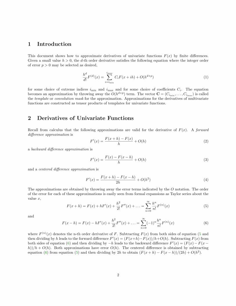
This document shows how to approximate derivatives of univariate functions F (x) by finite differences.Given a small value h > 0, the d-th order derivative satisfies the following equation where the integer orderof error p > 0 may be selected as desired,

hd

d!F (d)(x) =

imax∑i=imin

CiF (x + ih) + O(hd+p) (1)

for some choice of extreme indices imin and imax and for some choice of coefficients Ci. The equationbecomes an approximation by throwing away the O(hd+p) term. The vector C = (Cimin , . . . , Cimax) is calledthe template or convolution mask for the approximation. Approximations for the derivatives of multivariatefunctions are constructed as tensor products of templates for univariate functions.

2 Derivatives of Univariate Functions

Recall from calculus that the following approximations are valid for the derivative of F (x). A forwarddifference approximation is

F ′(x) =F (x + h)− F (x)

h+ O(h) (2)

a backward difference approximation is

F ′(x) =F (x)− F (x− h)

h+ O(h) (3)

and a centered difference approximation is

F ′(x) =F (x + h)− F (x− h)

2h+ O(h2) (4)

The approximations are obtained by throwing away the error terms indicated by the O notation. The orderof the error for each of these approximations is easily seen from formal expansions as Taylor series about thevalue x,

F (x + h) = F (x) + hF ′(x) +h2

2!F ′′(x) + . . . =

∞∑n=0

hn

n!F (n)(x) (5)

and

F (x− h) = F (x)− hF ′(x) +h2

2!F ′′(x) + . . . =

∞∑n=0

(−1)nhn

n!F (n)(x) (6)

where F (n)(x) denotes the n-th order derivative of F . Subtracting F (x) from both sides of equation (5 andthen dividing by h leads to the forward difference F ′(x) = (F (x+h)−F (x))/h+O(h). Subtracting F (x) fromboth sides of equation (6) and then dividing by −h leads to the backward difference F ′(x) = (F (x)−F (x−h))/h + O(h). Both approximations have error O(h). The centered difference is obtained by subtractingequation (6) from equation (5) and then dividing by 2h to obtain (F (x + h)− F (x− h))/(2h) + O(h2).

2

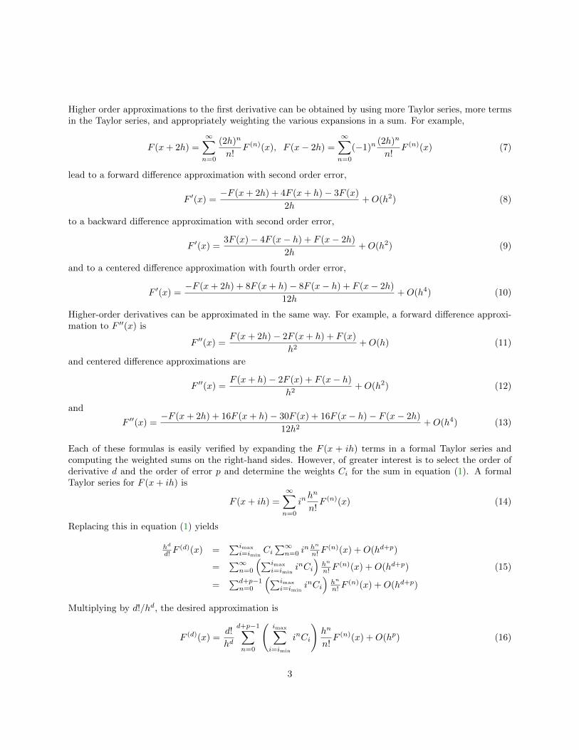
Higher order approximations to the first derivative can be obtained by using more Taylor series, more termsin the Taylor series, and appropriately weighting the various expansions in a sum. For example,

F (x + 2h) =

∞∑n=0

(2h)n

n!F (n)(x), F (x− 2h) =

∞∑n=0

(−1)n(2h)n

n!F (n)(x) (7)

lead to a forward difference approximation with second order error,

F ′(x) =−F (x + 2h) + 4F (x + h)− 3F (x)

2h+ O(h2) (8)

to a backward difference approximation with second order error,

F ′(x) =3F (x)− 4F (x− h) + F (x− 2h)

2h+ O(h2) (9)

and to a centered difference approximation with fourth order error,

F ′(x) =−F (x + 2h) + 8F (x + h)− 8F (x− h) + F (x− 2h)

12h+ O(h4) (10)

Higher-order derivatives can be approximated in the same way. For example, a forward difference approxi-mation to F ′′(x) is

F ′′(x) =F (x + 2h)− 2F (x + h) + F (x)

h2+ O(h) (11)

and centered difference approximations are

F ′′(x) =F (x + h)− 2F (x) + F (x− h)

h2+ O(h2) (12)

and

F ′′(x) =−F (x + 2h) + 16F (x + h)− 30F (x) + 16F (x− h)− F (x− 2h)

12h2+ O(h4) (13)

Each of these formulas is easily verified by expanding the F (x + ih) terms in a formal Taylor series andcomputing the weighted sums on the right-hand sides. However, of greater interest is to select the order ofderivative d and the order of error p and determine the weights Ci for the sum in equation (1). A formalTaylor series for F (x + ih) is

F (x + ih) =

∞∑n=0

inhn

n!F (n)(x) (14)

Replacing this in equation (1) yields

hd

d! F(d)(x) =

∑imax

i=iminCi

∑∞n=0 i

n hn

n! F(n)(x) + O(hd+p)

=∑∞

n=0

(∑imax

i=imininCi

)hn

n! F(n)(x) + O(hd+p)

=∑d+p−1

n=0

(∑imax

i=imininCi

)hn

n! F(n)(x) + O(hd+p)

(15)

Multiplying by d!/hd, the desired approximation is

F (d)(x) =d!

hd

d+p−1∑n=0

(imax∑

i=imin

inCi

)hn

n!F (n)(x) + O(hp) (16)

3

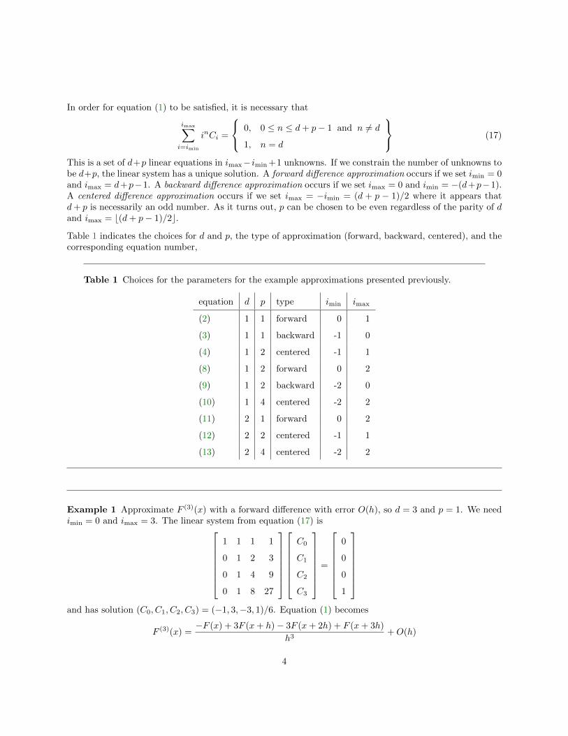
In order for equation (1) to be satisfied, it is necessary that

imax∑i=imin

inCi =

0, 0 ≤ n ≤ d + p− 1 and n 6= d

1, n = d

(17)

This is a set of d+p linear equations in imax− imin +1 unknowns. If we constrain the number of unknowns tobe d+p, the linear system has a unique solution. A forward difference approximation occurs if we set imin = 0and imax = d+p−1. A backward difference approximation occurs if we set imax = 0 and imin = −(d+p−1).A centered difference approximation occurs if we set imax = −imin = (d + p − 1)/2 where it appears thatd + p is necessarily an odd number. As it turns out, p can be chosen to be even regardless of the parity of dand imax = b(d + p− 1)/2c.

Table 1 indicates the choices for d and p, the type of approximation (forward, backward, centered), and thecorresponding equation number,

Table 1 Choices for the parameters for the example approximations presented previously.

equation d p type imin imax

(2) 1 1 forward 0 1

(3) 1 1 backward -1 0

(4) 1 2 centered -1 1

(8) 1 2 forward 0 2

(9) 1 2 backward -2 0

(10) 1 4 centered -2 2

(11) 2 1 forward 0 2

(12) 2 2 centered -1 1

(13) 2 4 centered -2 2

Example 1 Approximate F (3)(x) with a forward difference with error O(h), so d = 3 and p = 1. We needimin = 0 and imax = 3. The linear system from equation (17) is

1 1 1 1

0 1 2 3

0 1 4 9

0 1 8 27

C0

C1

C2

C3

=

0

0

0

1

and has solution (C0, C1, C2, C3) = (−1, 3,−3, 1)/6. Equation (1) becomes

F (3)(x) =−F (x) + 3F (x + h)− 3F (x + 2h) + F (x + 3h)

h3+ O(h)

4

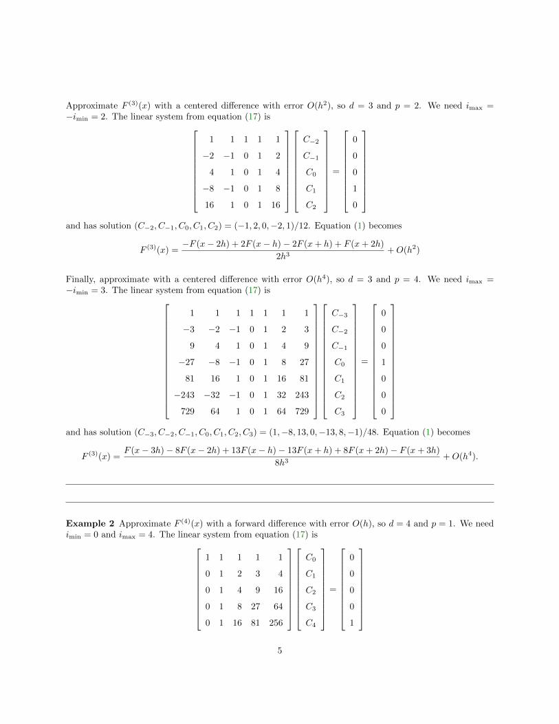
Approximate F (3)(x) with a centered difference with error O(h2), so d = 3 and p = 2. We need imax =−imin = 2. The linear system from equation (17) is

1 1 1 1 1

−2 −1 0 1 2

4 1 0 1 4

−8 −1 0 1 8

16 1 0 1 16

C−2

C−1

C0

C1

C2

=

0

0

0

1

0

and has solution (C−2, C−1, C0, C1, C2) = (−1, 2, 0,−2, 1)/12. Equation (1) becomes

F (3)(x) =−F (x− 2h) + 2F (x− h)− 2F (x + h) + F (x + 2h)

2h3+ O(h2)

Finally, approximate with a centered difference with error O(h4), so d = 3 and p = 4. We need imax =−imin = 3. The linear system from equation (17) is

1 1 1 1 1 1 1

−3 −2 −1 0 1 2 3

9 4 1 0 1 4 9

−27 −8 −1 0 1 8 27

81 16 1 0 1 16 81

−243 −32 −1 0 1 32 243

729 64 1 0 1 64 729

C−3

C−2

C−1

C0

C1

C2

C3

=

0

0

0

1

0

0

0

and has solution (C−3, C−2, C−1, C0, C1, C2, C3) = (1,−8, 13, 0,−13, 8,−1)/48. Equation (1) becomes

F (3)(x) =F (x− 3h)− 8F (x− 2h) + 13F (x− h)− 13F (x + h) + 8F (x + 2h)− F (x + 3h)

8h3+ O(h4).

Example 2 Approximate F (4)(x) with a forward difference with error O(h), so d = 4 and p = 1. We needimin = 0 and imax = 4. The linear system from equation (17) is

1 1 1 1 1

0 1 2 3 4

0 1 4 9 16

0 1 8 27 64

0 1 16 81 256

C0

C1

C2

C3

C4

=

0

0

0

0

1

5

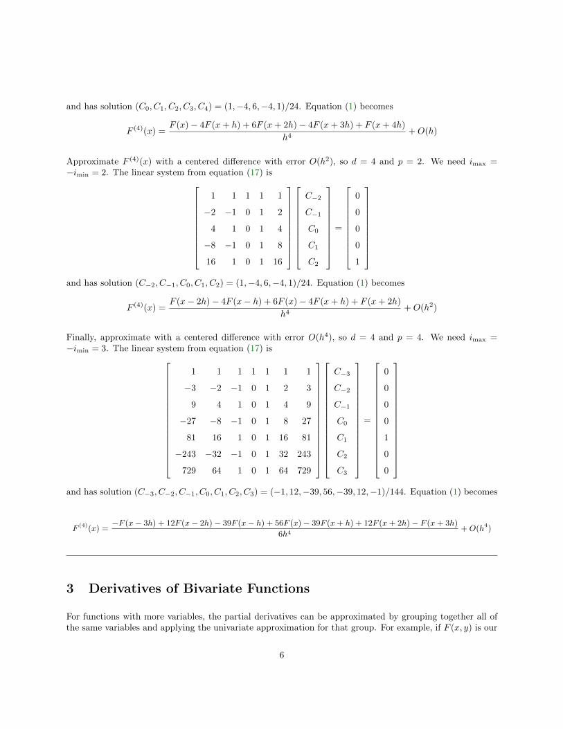
and has solution (C0, C1, C2, C3, C4) = (1,−4, 6,−4, 1)/24. Equation (1) becomes

F (4)(x) =F (x)− 4F (x + h) + 6F (x + 2h)− 4F (x + 3h) + F (x + 4h)

h4+ O(h)

Approximate F (4)(x) with a centered difference with error O(h2), so d = 4 and p = 2. We need imax =−imin = 2. The linear system from equation (17) is

1 1 1 1 1

−2 −1 0 1 2

4 1 0 1 4

−8 −1 0 1 8

16 1 0 1 16

C−2

C−1

C0

C1

C2

=

0

0

0

0

1

and has solution (C−2, C−1, C0, C1, C2) = (1,−4, 6,−4, 1)/24. Equation (1) becomes

F (4)(x) =F (x− 2h)− 4F (x− h) + 6F (x)− 4F (x + h) + F (x + 2h)

h4+ O(h2)

Finally, approximate with a centered difference with error O(h4), so d = 4 and p = 4. We need imax =−imin = 3. The linear system from equation (17) is

1 1 1 1 1 1 1

−3 −2 −1 0 1 2 3

9 4 1 0 1 4 9

−27 −8 −1 0 1 8 27

81 16 1 0 1 16 81

−243 −32 −1 0 1 32 243

729 64 1 0 1 64 729

C−3

C−2

C−1

C0

C1

C2

C3

=

0

0

0

0

1

0

0

and has solution (C−3, C−2, C−1, C0, C1, C2, C3) = (−1, 12,−39, 56,−39, 12,−1)/144. Equation (1) becomes

F (4)(x) =−F (x− 3h) + 12F (x− 2h)− 39F (x− h) + 56F (x)− 39F (x+ h) + 12F (x+ 2h)− F (x+ 3h)

6h4+O(h4)

3 Derivatives of Bivariate Functions

For functions with more variables, the partial derivatives can be approximated by grouping together all ofthe same variables and applying the univariate approximation for that group. For example, if F (x, y) is our

6

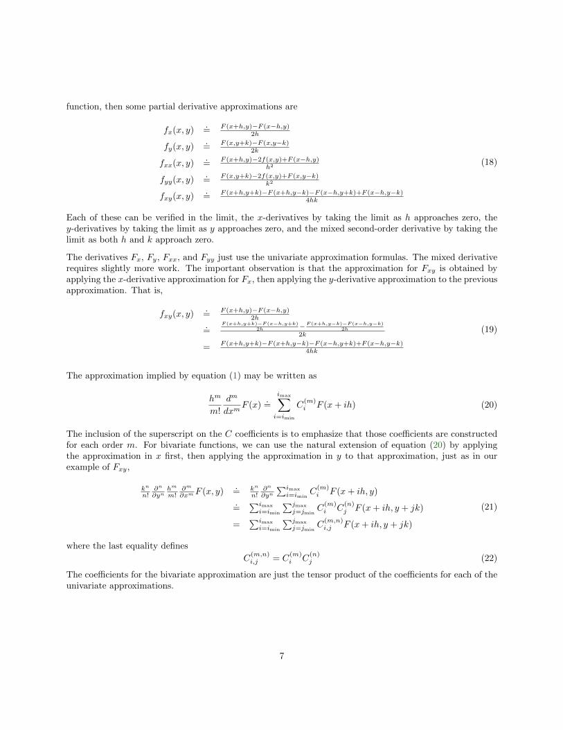
function, then some partial derivative approximations are

fx(x, y).= F (x+h,y)−F (x−h,y)

2h

fy(x, y).= F (x,y+k)−F (x,y−k)

2k

fxx(x, y).= F (x+h,y)−2f(x,y)+F (x−h,y)

h2

fyy(x, y).= F (x,y+k)−2f(x,y)+F (x,y−k)

k2

fxy(x, y).= F (x+h,y+k)−F (x+h,y−k)−F (x−h,y+k)+F (x−h,y−k)

4hk

(18)

Each of these can be verified in the limit, the x-derivatives by taking the limit as h approaches zero, they-derivatives by taking the limit as y approaches zero, and the mixed second-order derivative by taking thelimit as both h and k approach zero.

The derivatives Fx, Fy, Fxx, and Fyy just use the univariate approximation formulas. The mixed derivativerequires slightly more work. The important observation is that the approximation for Fxy is obtained byapplying the x-derivative approximation for Fx, then applying the y-derivative approximation to the previousapproximation. That is,

fxy(x, y).= F (x+h,y)−F (x−h,y)

2h

.=

F (x+h,y+k)−F (x−h,y+k)2h −F (x+h,y−k)−F (x−h,y−k)

2h

2k

= F (x+h,y+k)−F (x+h,y−k)−F (x−h,y+k)+F (x−h,y−k)4hk

(19)

The approximation implied by equation (1) may be written as

hm

m!

dm

dxmF (x)

.=

imax∑i=imin

C(m)i F (x + ih) (20)

The inclusion of the superscript on the C coefficients is to emphasize that those coefficients are constructedfor each order m. For bivariate functions, we can use the natural extension of equation (20) by applyingthe approximation in x first, then applying the approximation in y to that approximation, just as in ourexample of Fxy,

kn

n!∂n

∂ynhm

m!∂m

∂xmF (x, y).= kn

n!∂n

∂yn

∑imax

i=iminC

(m)i F (x + ih, y)

.=

∑imax

i=imin

∑jmax

j=jminC

(m)i C

(n)j F (x + ih, y + jk)

=∑imax

i=imin

∑jmax

j=jminC

(m,n)i,j F (x + ih, y + jk)

(21)

where the last equality defines

C(m,n)i,j = C

(m)i C

(n)j (22)

The coefficients for the bivariate approximation are just the tensor product of the coefficients for each of theunivariate approximations.

7

4 Derivatives of Multivariate Functions

The approximation concept extends to any number of variables. Let (x1, . . . , xn) be those variables and letF (x1, . . . , xn) be the function to approximate. The approximation is

(hm11

m1!

∂m1

∂xm11

· · · hmnn

mn!

∂mn

∂xmn1

)F (x1, . . . , xn)

.=

imax1∑

i1=imin1

· · ·imaxn∑

in=iminn

C(m1,...,mn)(i1,...,in)

F (x1 + i1h1, . . . , xn + inhn) (23)

whereC

(m1,...,mn)(i1,...,in)

= C(m1)i1

· · ·C(mn)in

(24)

is a tensor product of the coefficients of the n univariate approximations.

8