FINITE-VOLUME METHODS

Milovan Perić

CoMeT Continuum Mechanics Technologies GmbH

milovan@continuummechanicstechnologies.de

Introduction

• FV is the most widely used method in CFD (all major commercial codes are based on FV-approach)…

• Starting point: conservation equations in integral form, e.g. generic steady-state conservation equation:

• FV-method is applicable to any grid type (structured or unstructured).

• It requires approximation of derivatives, surface and volume integrals, and interpolation at points other than cell centroids…

• For each control volume, one algebraic equation is obtained…• For the whole solution domain, a system of algebraic equations

needs to be solved.

FV-Methods for Arbitrary CVs – I

• In FV-methods, CVs can be of an arbitrary polyhedral shape.

• The shape of CV-faces is not important when vertices are connected by straight lines and Cartesian base vectors are used.

• Here unstructured grids are considered; structured grid is a special case of an unstructured grid…

• Data is organized in lists: vertex, face and cell list.

• Vertex list contains:

– Vertex index

– Coordinates (x,y,z) of the vertex location.

• The order in which vertices are listed is arbitrary.

FV-Methods for Arbitrary CVs – II

• Face list contains:– Face index;

– Number of vertices defining the face;

– List of indices of vertices which define the face, in the order in which they are connected (counterclockwise; the last listed vertex connects to the first one to close the polygon);

– Coordinates of the face centroid;

– Surface-vector components (face projections to coordinate planes);

– Indices of cells on either side of the face (surface vector points from the first to the second cell);

– Coefficients for the Matrix A multiplying neighbor variable value.

FV-Methods for Arbitrary CVs – III

• Cell list contains:– Cell index;

– Number of faces enclosing the cell;

– List of indices of faces which enclose the cell, in arbitrary order;

– Coordinates of the cell centroid;

– Cell volume;

– Variable values and fluid properties;

– Coefficient AP for the Matrix A and the source term QP .

• Unstructured grids can be: tetrahedral, with mixed shapes up to hexahedra, or arbitrary polyhedral.

• Polyhedra are usually obtained by “dualizing” tetrahedra…

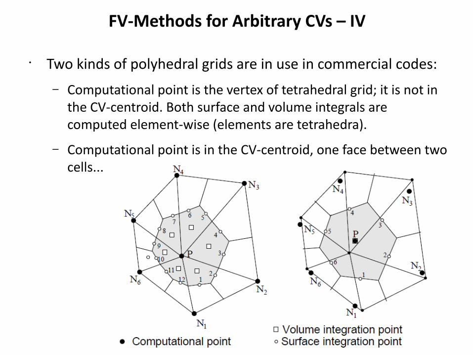
FV-Methods for Arbitrary CVs – IV

• Two kinds of polyhedral grids are in use in commercial codes:– Computational point is the vertex of tetrahedral grid; it is not in

the CV-centroid. Both surface and volume integrals are computed element-wise (elements are tetrahedra).

– Computational point is in the CV-centroid, one face between two cells...

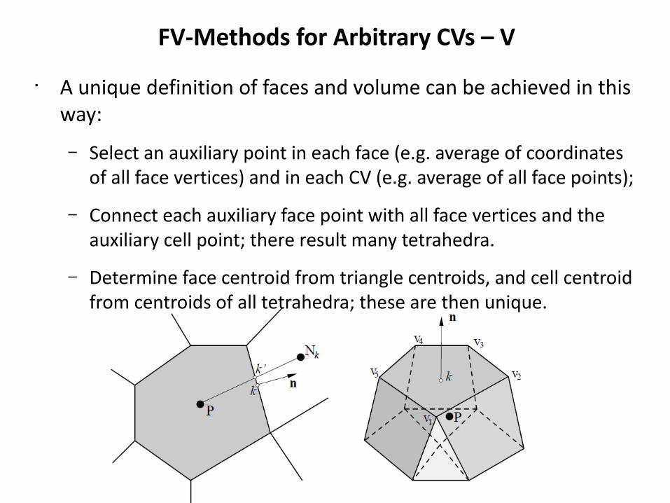
FV-Methods for Arbitrary CVs – V

• A unique definition of faces and volume can be achieved in this way:

– Select an auxiliary point in each face (e.g. average of coordinates of all face vertices) and in each CV (e.g. average of all face points);

– Connect each auxiliary face point with all face vertices and the auxiliary cell point; there result many tetrahedra.

– Determine face centroid from triangle centroids, and cell centroid from centroids of all tetrahedra; these are then unique.

Approximation of Surface Integrals – I

• The integral over closed surface = sum of integrals over faces:

• Here is the component of convection or diffusion vector in the direction normal to cell face, or .

• Two levels of approximation are required:– Approximation of the integral;– Interpolation to integration points in the face (convection)

or approximation of the derivative in the direction normal to the face (diffusion).

• The simplest second-order approximation is the midpoint-rule:

Approximation of Surface Integrals – II • Midpoint rule is the simplest 2nd-order approximation of

surface integrals that is applicable to any polygonal face.

• For any flux vector f,

Approximation of Volume Integrals

• Midpoint rule is the simplest 2nd-order approximation of volume integrals that is applicable to any polyhedral control volume.

• For example, for source terms:

• No interpolation is necessary, but some source terms do require gradients to be approximated at CV-centroid.

• Second order is lost if P is not at the CV-centroid.

Interpolation Schemes – I

• There are many options for computing variable values at face centroid; e.g., linear extrapolation from P:

• Another option is linear extrapolation from Nk, (i.e., linear upwind scheme), or weighting of the two (linear interpolation).

• Simple interpolation delivers value at k’:

Interpolation Schemes – II

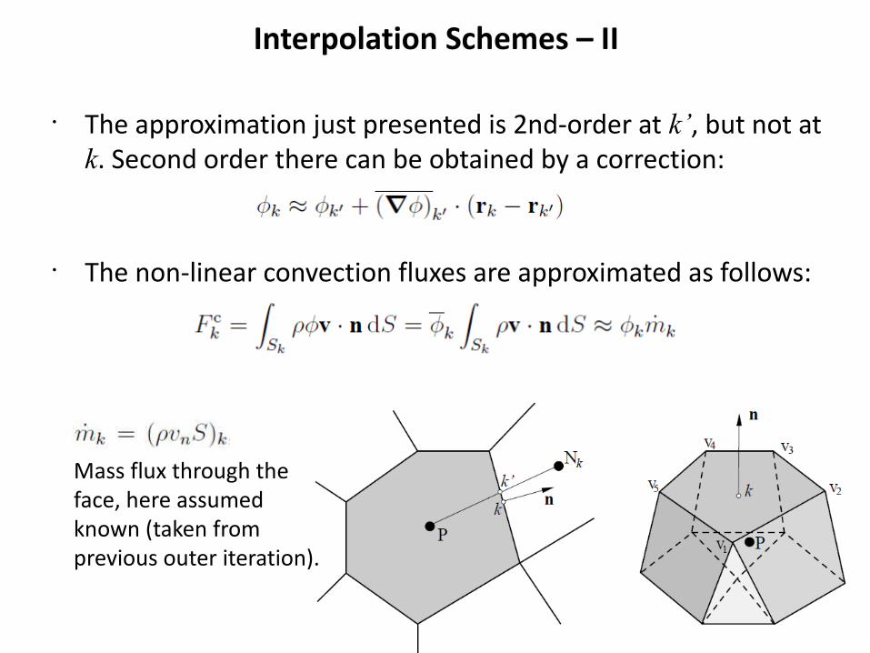
• The approximation just presented is 2nd-order at k’, but not at k. Second order there can be obtained by a correction:

• The non-linear convection fluxes are approximated as follows:

Mass flux through the face, here assumed known (taken from previous outer iteration).

Interpolation Schemes – II

• The approximation just presented is 2nd-order at k’, but not at k. Second order there can be obtained by a correction:

• The non-linear convection fluxes are approximated as follows:

Mass flux through the face, here assumed known (taken from previous outer iteration).

Differentiation Schemes – I

• Gradient at face centroid is needed for diffusive flux:

• Simple central-difference approximation,

is 2nd-order accurate when the line connecting CV-centroids passes through face centroid and is orthogonal to the face.

• A 2nd-order approximation for any situation can be obtained:

– by using coordinate transformation (as in FD-methods);

– by defining auxiliary points on face normal and using extrapolation from CV-centroids.

Differentiation Schemes – II

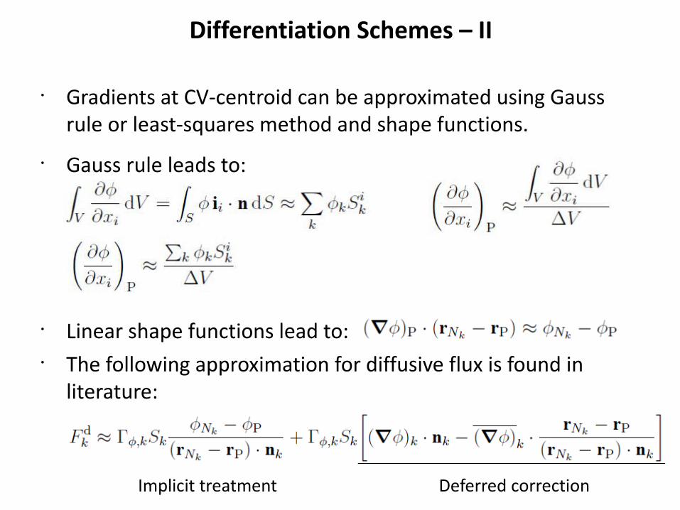
• Gradients at CV-centroid can be approximated using Gauss rule or least-squares method and shape functions.

• Gauss rule leads to:

• Linear shape functions lead to:• The following approximation for diffusive flux is found in

literature:

Deferred correctionImplicit treatment

Differentiation Schemes – III

• The simplest 2nd-order approximation is obtained using auxiliary nodes:

• Variable values at auxiliary nodes can be expressed as:

• leading to:

Non-Conformal Grid Block Interfaces – I

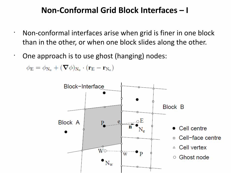
• Non-conformal interfaces arise when grid is finer in one block than in the other, or when one block slides along the other.

• One approach is to use ghost (hanging) nodes:

Non-Conformal Grid Block Interfaces – II

• The same approach applies to node W for cell P in block B.

• Other interpolations are also possible…

• Ghost-node values can be updated after each inner or outer iteration (or in a mixed way)…

• The method is not conservative, unless correction is applied…

Non-Conformal Grid Block Interfaces – III

• Another (conservative) treatment is to map CV-faces from two sides along interface and identify parts of interface which are common to two cells on either side…

• Cells along interface then have more faces and neighbors…

• A special data structure is needed to handle this situation (as for unstructured grids)…

Non-Conformal Grid Block Interfaces – IV

• The original faces are not used in discretization; the coefficient AE for the shaded face of block A is thus zero.

• A list of interface faces is created, which contains:– The indices of the left and right cell that share the face;– The coordinates of face centroid and surface vector components;– The coefficients AR for left cell and AL for right cell.

For sliding grids, face mapping and update of the interface list needs to be done in each time step.

Iterative solver adapted as for parallel computing.

Advantages of FV-Methods

• Most CFD-codes used in industry have been written by engineers – for engineers...

• Most of these codes are based on FV-method (FLUENT, STAR-CD, STAR-CCM+, CFX, OpenFOAM etc.).

• All these codes use midpoint-rule approximation for surface and volume integrals – so they are at most 2nd-order accurate.

• Approximations of gradients are also at most of 2nd-order...

• Some codes use higher-order interpolation (e.g. quadratic or cubic).

• The main reasons for above choices: simplicity, applicability to arbitrary polyhedra, easy coding, easy extraction of data of engineering interest (forces, fluxes etc.), easy code maintenance.

Disadvantages of FV-Methods

• The main disadvantage of FV-methods is the complexity of extension to orders higher than 2nd:

– Approximation of integrals becomes much more complicated (need more than one integration point – in 3D, many more...);

– Interpolation becomes more complicated (must be of at least the same order as integral approximaation);

– Approximation of gradients becomes much more complicated...

– Treatment of boundary conditions becomes more complicated (higher-order one-sided approximations are needed)...

• FV-methods of order higher than 2nd have been published mostly for two-dimensional problems...

Higher-Order Approximations – I

• A fourth-order approximation of surface integral in 2D is the Simpson-rule:

• To retain fourth order, has to be interpolated to face center and cell vertices with approximations of at least fourth order.

Higher-Order Approximations – II • Cubic interpolation in 2D (fit to four nodes):

• For a uniform Cartesian grid, one obtains:

• One can also fit cubic polynomial to 2 nodal values and two derivatives (for face e, using nodes P and E – compact scheme):

• The first term on r.h.s. is the 2nd-order CDS – the rest is the correction to achieve 4th-order approximation.

Uniform Cartesian grid

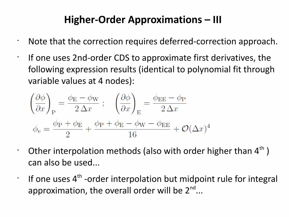
• Note that the correction requires deferred-correction approach.• If one uses 2nd-order CDS to approximate first derivatives, the

following expression results (identical to polynomial fit through variable values at 4 nodes):

• Other interpolation methods (also with order higher than 4th ) can also be used...

• If one uses 4th -order interpolation but midpoint rule for integral approximation, the overall order will be 2nd...

Higher-Order Approximations – III

Higher-Order Approximations – IV

• From a cubic polynomial fit to 4 nodal variable values, one can obtain the derivative at face center:

• For a uniform Cartesian grid, one obtains:

• By fitting a cubic polynomial to variable values and derivatives at 2 nodes, one obtains:

The first term on r.h.s. is the 2nd-order approximation; the rest is a 4th -order correction, which can be treated explicitly (deferred corr.)

Higher-Order Approximations – V

• In 2D, a 4th-order approximation of volume integral can be constructed using a bi-quadratic shape function (requires evaluation of function at 9 locations):

• For a 2D Cartesian grid, the following expressions result:

• In 3D and for arbitrary polyhedral CVs, derivation of 4th-order approximations would be very complicated...

• Finite-difference methods of order higher than 2nd are easier to construct than finite-volume methods of the same order...

What is CFD Nowadays Used for? - I

External aerodynamics(bicycles, motorcycles, cars, trucks, trains...).

LES, ca. 200 mio. CVs

Heat management (all equipment using internal combustion engines, gas turbines etc.).

What is CFD Nowadays Used for? - II

Aerospace (airplanes,rockets, missiles, helicopters etc.) - optimization of lift, drag, stability etc.

What is CFD Nowadays Used for? - V

Lifeboat launching from an offshore platform: safety analysis for boat and passengers...

Electronics cooling

Maritime applications

Biomedical applications