Embed Size (px)
Citation preview

FIRST DETERMINATION OF THE 8Li VALENCE
NEUTRON ASYMPTOTIC NORMALIZATION
COEFFICIENT USING THE 7Li(8Li,7Li)8Li REACTION
by
Derek Howell
B.Sc., Simon Fraser University, 2005
a Thesis submitted in partial fulfillment
of the requirements for the degree of
Doctor of Philosophy
in the
Department of Physics
Faculty of Science
c© Derek Howell 2013
SIMON FRASER UNIVERSITY
Spring 2013
All rights reserved.
However, in accordance with the Copyright Act of Canada, this work may be
reproduced without authorization under the conditions for “Fair Dealing.”
Therefore, limited reproduction of this work for the purposes of private study,
research, criticism, review and news reporting is likely to be in accordance
with the law, particularly if cited appropriately.

APPROVAL
Name: Derek Howell
Degree: Doctor of Philosophy
Title of Thesis: First Determination of the 8Li Valence Neutron Asymptotic
Normalization Coefficient using the 7Li(8Li,7Li)8Li reaction
Examining Committee: Dr. Sarah Johnson,
Senior Lecturer
Chair
Dr. Dugan O’Neil (Senior Supervisor),
Associate Professor
Dr. Barry Davids (Co-Supervisor),
Adjunct Professor
Dr. Levon Pogosian (Supervisor),
Associate Professor
Dr. Eldon Emberly (Internal Examiner),
Associate Professor
Dr. Alan Chen (External Examiner),
Associate Professor, Physics and Astronomy
McMaster University
Date Approved: March 19th, 2013
ii

Partial Copyright Licence

Abstract
Solar neutrino experiments have often been plagued with large uncertainties. With the
recent results from the Borexino Collaboration, for the first time the total uncertainty in
the 7Be solar neutrino flux measurement is smaller than the uncertainty of standard solar
model (SSM) predictions.
Improvement in neutrino experiments must be followed by refinements to the SSM; to
do so requires reduced uncertainties on the parameters used in SSM calculations. One such
value is the astrophysical S-factor describing the 7Be(p,γ)8B reaction, S17(0).
We report here a determination of the asymptotic normalization coefficient (ANC) of
the valence neutron in 8Li from a measurement of the angular distribution of the single
neutron transfer between 8Li and 7Li via the 7Li(8Li,7Li)8Li reaction at 11 MeV. Using
isospin symmetry the 8B ANC has also been calculated and used to infer a value for S17(0)
of 20.2± 4.4 eV b.
iii

To my wife Lisa. Without her love and support, none of this would have been possible.
iv

“Wonder implies the desire to learn”
— Aristotle
v

Acknowledgments
To begin I would like to thank Barry Davids for his guidance and advice that helped me
along with every step. Thanks must also go to Ritu Kanungo and Pat Walden for their
extensive help with the experiment. Thanks to Tom Davinson for sharing his expertise of
the TUDA systems and help in solving system and detector mysteries I would never have
been able to figure out on my own. Thanks to Ian Thompson for his help in understanding
FRESCO and all the calculations that at first seemed overwhelming. Finally, thanks to
countless others who helped. Your help, support and advice, however small, was invaluable.
vi

Contents
Approval ii
Abstract iii
Dedication iv
Quotation v
Acknowledgments vi
Contents vii
List of Tables xi
List of Figures xiv
1 Introduction 1
1.1 Nuclear Astrophysics . . . . . . . . . . . . . . . . . . . . . . . . . . . . . . . . 1
1.2 Thermonuclear Reactions in a Stellar Environment . . . . . . . . . . . . . . . 2
1.2.1 The Proton-Proton Chains . . . . . . . . . . . . . . . . . . . . . . . . 4
1.2.2 CNO cycles . . . . . . . . . . . . . . . . . . . . . . . . . . . . . . . . . 8
1.3 Neutrinos . . . . . . . . . . . . . . . . . . . . . . . . . . . . . . . . . . . . . . 8
1.3.1 Solar Neutrinos . . . . . . . . . . . . . . . . . . . . . . . . . . . . . . . 10
1.4 S17(0) History and Background . . . . . . . . . . . . . . . . . . . . . . . . . . 12
2 Theory 14
2.1 Stellar Reaction Rates . . . . . . . . . . . . . . . . . . . . . . . . . . . . . . . 14
vii

2.1.1 Energy of a Star . . . . . . . . . . . . . . . . . . . . . . . . . . . . . . 15
2.1.2 Tunnelling in a Star . . . . . . . . . . . . . . . . . . . . . . . . . . . . 16
2.1.3 Astrophysical S-Factor . . . . . . . . . . . . . . . . . . . . . . . . . . . 17
2.1.4 The Gamow Window . . . . . . . . . . . . . . . . . . . . . . . . . . . . 19
2.2 Scattering Theory . . . . . . . . . . . . . . . . . . . . . . . . . . . . . . . . . 22
2.2.1 Schrodinger Equation for a Central Potential . . . . . . . . . . . . . . 22
2.2.2 Differential Cross Section and Scattering amplitudes . . . . . . . . . . 24
2.2.3 Phase shifts . . . . . . . . . . . . . . . . . . . . . . . . . . . . . . . . . 26
2.2.4 DWBA . . . . . . . . . . . . . . . . . . . . . . . . . . . . . . . . . . . 29
2.2.5 Partial-wave expansions . . . . . . . . . . . . . . . . . . . . . . . . . . 30
2.3 Indirect Methods . . . . . . . . . . . . . . . . . . . . . . . . . . . . . . . . . . 32
2.3.1 Transfer Reactions . . . . . . . . . . . . . . . . . . . . . . . . . . . . . 32
2.3.2 Asymptotic Normalization Coefficients . . . . . . . . . . . . . . . . . . 35
2.3.3 Extraction of the ANC . . . . . . . . . . . . . . . . . . . . . . . . . . . 38
3 Experimental Procedure 40
3.1 TRIUMF . . . . . . . . . . . . . . . . . . . . . . . . . . . . . . . . . . . . . . 40
3.2 RIB facilities . . . . . . . . . . . . . . . . . . . . . . . . . . . . . . . . . . . . 41
3.2.1 Beam Production . . . . . . . . . . . . . . . . . . . . . . . . . . . . . . 41
3.2.2 Beam Transport and acceleration . . . . . . . . . . . . . . . . . . . . . 42
3.3 TUDA . . . . . . . . . . . . . . . . . . . . . . . . . . . . . . . . . . . . . . . . 42
3.3.1 Detectors . . . . . . . . . . . . . . . . . . . . . . . . . . . . . . . . . . 43
3.4 Experiment Setup . . . . . . . . . . . . . . . . . . . . . . . . . . . . . . . . . 46
3.5 Instrumentation, data acquisition and detector calibration . . . . . . . . . . . 47
3.6 The 7Li(8Li,7Li)8Li reaction . . . . . . . . . . . . . . . . . . . . . . . . . . . . 50
3.6.1 Peripheral nature of the reaction . . . . . . . . . . . . . . . . . . . . . 50
4 Analysis Software 54
4.1 MIDAS . . . . . . . . . . . . . . . . . . . . . . . . . . . . . . . . . . . . . . . 54
4.2 ROOT . . . . . . . . . . . . . . . . . . . . . . . . . . . . . . . . . . . . . . . . 55
4.2.1 Framework . . . . . . . . . . . . . . . . . . . . . . . . . . . . . . . . . 55
4.2.2 Histograms . . . . . . . . . . . . . . . . . . . . . . . . . . . . . . . . . 56
4.2.3 Fitting Histograms . . . . . . . . . . . . . . . . . . . . . . . . . . . . . 56
4.3 FRESCO . . . . . . . . . . . . . . . . . . . . . . . . . . . . . . . . . . . . . . 57
viii
4.3.1 7Li(8Li,7Li)8Li . . . . . . . . . . . . . . . . . . . . . . . . . . . . . . . 57
4.4 SFRESCO . . . . . . . . . . . . . . . . . . . . . . . . . . . . . . . . . . . . . . 59
4.4.1 p + 112Cd elastic scattering . . . . . . . . . . . . . . . . . . . . . . . . 59
4.4.2 Minuit Error . . . . . . . . . . . . . . . . . . . . . . . . . . . . . . . . 62
5 Data Analysis 63
5.1 Detector Calibration . . . . . . . . . . . . . . . . . . . . . . . . . . . . . . . . 63
5.1.1 Energy and Time calibration . . . . . . . . . . . . . . . . . . . . . . . 64
5.1.2 Beam Offset . . . . . . . . . . . . . . . . . . . . . . . . . . . . . . . . . 64
5.1.3 Detector Geometry . . . . . . . . . . . . . . . . . . . . . . . . . . . . . 67
5.1.4 Split Events . . . . . . . . . . . . . . . . . . . . . . . . . . . . . . . . . 68
5.1.5 S2 Crosstalk . . . . . . . . . . . . . . . . . . . . . . . . . . . . . . . . 69
5.2 Data Reduction . . . . . . . . . . . . . . . . . . . . . . . . . . . . . . . . . . . 73
5.2.1 Background Reduction . . . . . . . . . . . . . . . . . . . . . . . . . . . 73
5.2.2 S2 data reduction . . . . . . . . . . . . . . . . . . . . . . . . . . . . . 78
5.2.3 Fitting the S2 data . . . . . . . . . . . . . . . . . . . . . . . . . . . . . 80
5.2.4 Error estimates . . . . . . . . . . . . . . . . . . . . . . . . . . . . . . . 82
5.3 SFRESCO Fit . . . . . . . . . . . . . . . . . . . . . . . . . . . . . . . . . . . 85
6 Angular Distribution Analysis 86
6.1 Binding Potential and Single Particle ANC . . . . . . . . . . . . . . . . . . . 86
6.2 Data fitting . . . . . . . . . . . . . . . . . . . . . . . . . . . . . . . . . . . . . 88
6.2.1 Initial fit . . . . . . . . . . . . . . . . . . . . . . . . . . . . . . . . . . 88
6.2.2 Secondary Fit . . . . . . . . . . . . . . . . . . . . . . . . . . . . . . . . 89
7 Results and Discussion 92
7.1 Previous Results . . . . . . . . . . . . . . . . . . . . . . . . . . . . . . . . . . 92
7.1.1 ANC . . . . . . . . . . . . . . . . . . . . . . . . . . . . . . . . . . . . . 92
7.1.2 S factor . . . . . . . . . . . . . . . . . . . . . . . . . . . . . . . . . . . 93
7.2 New Results . . . . . . . . . . . . . . . . . . . . . . . . . . . . . . . . . . . . . 94
7.2.1 ANC . . . . . . . . . . . . . . . . . . . . . . . . . . . . . . . . . . . . . 94
7.2.2 S factor . . . . . . . . . . . . . . . . . . . . . . . . . . . . . . . . . . . 95
7.3 Future Work . . . . . . . . . . . . . . . . . . . . . . . . . . . . . . . . . . . . 96
7.4 Conclusion . . . . . . . . . . . . . . . . . . . . . . . . . . . . . . . . . . . . . 96
ix

Appendix A FRESCO 98
A.1 FRECO Examples . . . . . . . . . . . . . . . . . . . . . . . . . . . . . . . . . 98
A.1.1 Elastic scattering . . . . . . . . . . . . . . . . . . . . . . . . . . . . . . 98
A.1.2 Transfer Reaction . . . . . . . . . . . . . . . . . . . . . . . . . . . . . 100
A.2 Variable Descriptions . . . . . . . . . . . . . . . . . . . . . . . . . . . . . . . . 103
Appendix B FRESCO Input Code 107
B.1 Elastic Scattering . . . . . . . . . . . . . . . . . . . . . . . . . . . . . . . . . . 108
B.2 Transfer Reaction . . . . . . . . . . . . . . . . . . . . . . . . . . . . . . . . . . 109
B.3 7Li(8Li,7Li)8Li Transfer Reaction . . . . . . . . . . . . . . . . . . . . . . . . 111
B.4 p + 112Cd elastic scattering . . . . . . . . . . . . . . . . . . . . . . . . . . . . 113
B.5 SFRESCO . . . . . . . . . . . . . . . . . . . . . . . . . . . . . . . . . . . . . . 115
Appendix C MINUIT 116
C.1 MIGRAD . . . . . . . . . . . . . . . . . . . . . . . . . . . . . . . . . . . . . . 116
C.2 SCAN . . . . . . . . . . . . . . . . . . . . . . . . . . . . . . . . . . . . . . . . 117
Bibliography 118
x

List of Tables
1.1 Energy of emitted neutrinos from reactions in the pp chains. Reaction 3,
known as the hep reaction, has never been detected due to the extremely
small branching ratio and is only theorized at this time. . . . . . . . . . . . . 7
3.1 Physical dimensions for each element of a LEDA sector. Each element is a
strip along the sector with the given angular size, inner and outer radii, and
physical area. . . . . . . . . . . . . . . . . . . . . . . . . . . . . . . . . . . . . 45
3.2 Variation in the parametrization of potential 2 in Table 4.1 with correspond-
ing single particle ANC values. Included are the corresponding χ2 values
determined by comparison of the computed bound state wavefunction to the
VMC wavefunction of R. Wiringa [33] which may be seen in Figure 6.1. . . . 52
4.1 Interaction potentials used for FRESCO calculation of 7Li(8Li,7Li)8Li reac-
tion at 11 MeV. The “kp” value corresponds to the index of the potential
as it appears in the input file of Figure B.3. Real and imaginary depths, V
and W, are expressed in MeV. Radii and diffusenesses are in fm. The radii of
the optical potentials are reduced, and full radii follow the convention Ri =
ri(A1/3t +A
1/3p ) where i is either V or W. Potential 1 is the optical potential for
the interaction between the 7Li + 8Li nuclei. Potentials 2 and 4 are binding
potentials for the p3/2 and p1/2 orbitals respectively, and potential 10 is the
core-core interaction. . . . . . . . . . . . . . . . . . . . . . . . . . . . . . . . . 58
4.2 SFRESCO data types . . . . . . . . . . . . . . . . . . . . . . . . . . . . . . . 60
4.3 SFRESCO fit results for p + 112Cd elastic scattering from input files displayed
in Figures B.4 and B.6 . . . . . . . . . . . . . . . . . . . . . . . . . . . . . . . 62
xi

5.1 Kinematically calculated range of the recoil and ejectile angles in degrees
from the 7Li(8Li,7Li)8Li reaction. The LEDA detector covers a range from
36 to 60 degrees. . . . . . . . . . . . . . . . . . . . . . . . . . . . . . . . . . . 66
5.2 Calculated beam offset based on asymmetry of elastically scattered 19F events 66
5.3 Total number of events processed in the S2 detector prior to and following the
application of energy gates to the data. The final entry includes all events
after equal energy gates and corrections to events discussed due to energy
splitting between adjacent channels. . . . . . . . . . . . . . . . . . . . . . . . 69
5.4 Contributions to the error for the angular distribution data from the S2 and
LEDA detectors. . . . . . . . . . . . . . . . . . . . . . . . . . . . . . . . . . . 83
6.1 Binding potentials for the p3/2 orbital of the valence neutron of 8Li with
corresponding single particle ANC values from reference [34]. . . . . . . . . . 87
6.2 Parameters for the entrance and exit channel optical potential for the p3/2
orbital interaction between 8Li and 7Li. The fit parameters are the results
of an SFRESCO minimization to the dataset using initial parameters for the
potential taken from reference [34]. . . . . . . . . . . . . . . . . . . . . . . . . 89
6.3 Fit results from SFRESCO for the optical potential parameters, normaliza-
tion, and spectroscopic amplitude for the p3/2 orbital. Limits placed on the
parameters prior to performing the fit are indicated in the individual plots for
each parameter in Figure 6.2. Units for the depths are in MeV, the reduced
radii are in fm, and the diffusenesses are in fm. . . . . . . . . . . . . . . . . . 89
7.1 Calculated squares of ANCs (in fm−1) for p1/2 and p3/2 orbitals and their
sums. Calculations were performed with two NN potentials, V2 and MN. The
ratios of similar quantities for the mirror overlap are given for each potential
[46]. The average of the ratios of the two potentials is also given. . . . . . . . 93
A.1 Interaction potentials used for FRESCO calculation of 14N(7Be,8B)13C reac-
tion at 84 MeV. The “kp” value corresponds to the index of the potential as
it appears in the input file of Figure B.2. Potential depths are in MeV while
radii and diffusenesses are in fm. . . . . . . . . . . . . . . . . . . . . . . . . . 101
A.2 Different types of coupling given by the parameter “kind” in the “&COU-
PLING” heading. . . . . . . . . . . . . . . . . . . . . . . . . . . . . . . . . . . 102
xii

A.3 Integration and trace variables for the &FRESCO entry . . . . . . . . . . . . 103
A.4 Variables for the &PARTITIONS and &STATES entry . . . . . . . . . . . . . 104
A.5 Variables for the &POTENTIAL entry . . . . . . . . . . . . . . . . . . . . . . 105
A.6 Variables for the &OVERLAP entry . . . . . . . . . . . . . . . . . . . . . . . 105
A.7 Variables for the &COUPLING and &CFP entry . . . . . . . . . . . . . . . . 106
A.8 SFRESCO input commands . . . . . . . . . . . . . . . . . . . . . . . . . . . . 106
xiii

List of Figures
1.1 Binding Energy per Nucleon curve. Figure from Reference [3] . . . . . . . . . 3
1.2 Power liberated by the pp chains and one of the CNO cycles as a function of
temperature. The crossover point between the pp chains and the CNO cycles
is roughly at a mass of 1.5 times that of the Sun. The black dot indicates the
temperature of the Sun. Figure taken from Reference [1]. . . . . . . . . . . . 5
1.3 The pp chains with associated branching ratios applicable to the Sun[1].
While an α particle and 4He are the same the use of α in some reactions
is to highlight that this particle is acting as a catalyst and is not the 4He
produced in the chain. . . . . . . . . . . . . . . . . . . . . . . . . . . . . . . . 7
1.4 The C, N, and O isotopes serve as catalysts for the reaction shown in Equation
1.4. The CN cycle on the left and CNO cycle on the right are together referred
to as the CNO bicycle. . . . . . . . . . . . . . . . . . . . . . . . . . . . . . . . 9
1.5 The Solar neutrino energy spectrum for all neutrinos produced in the CNO
cycles and the pp chains with energies listed in Table 1.1 as predicted by the
SSM. Figure from Reference [12]. . . . . . . . . . . . . . . . . . . . . . . . . . 11
2.1 The cross section for the 7Be(p,γ)8B reaction from Reference [23]. The
coloured points represent data from three experiments. The solid curve is
a scaled calculation using the non-resonant Descouvemont and Baye (DB)
theory plus fitted 1+ and 3+ resonances. The dashed curve is the DB fit only,
while the lower solid line is the resonant contribution. . . . . . . . . . . . . . 18
2.2 The S-factor for the 7Be(p,γ)8B reaction from Reference [23]. The solid curve
is a scaled calculation using the non-resonant Descouvemont and Baye (DB)
theory plus fitted 1+ and 3+ resonances. The dashed curve is the DB fit only,
while the lower solid line is the resonant contribution. . . . . . . . . . . . . . 20
xiv

2.3 Overlap of the Maxwell-Boltzmann distribution with the penetration factor
to form the Gamow peak. . . . . . . . . . . . . . . . . . . . . . . . . . . . . . 21
2.4 Stripping reaction with associated coordinates for the reaction X+A→ Y +B
where X = Y + a , and B = A+ a with a being the transferred particle. . . . 33
3.1 ISAC experimental hall . . . . . . . . . . . . . . . . . . . . . . . . . . . . . . 41
3.2 TUDA chamber as arranged in the experiment. . . . . . . . . . . . . . . . . . 43
3.3 Image of the LEDA detector . . . . . . . . . . . . . . . . . . . . . . . . . . . . 44
3.4 Schematic setup of the electronics for the TUDA chamber. . . . . . . . . . . . 48
3.5 DWBA calculations for the 7Li(8Li,7Li)8Li reaction at 13 MeV normalized
to b4. Only the transfer cross section is shown with data sets labeled by the
corresponding binding potential parametrization of Table 3.2. Included are
enlargements of two sections at θ = 0 and θ = 180 in order to assess the
spread at each extreme. Figure from Reference [34] . . . . . . . . . . . . . . . 53
4.1 Data and calculations of proton scattering on 112Cd at 27.90 MeV with initial
and fitted potential parameters. . . . . . . . . . . . . . . . . . . . . . . . . . . 61
5.1 Elastic scattering of 8Li from 19F. The x-axis represents the S2 channel num-
ber starting at x=0 for sector 0 ring 0 and incrementing by ring (i.e. x=1
represents sector 0 ring 1, x=2 represents sector 0 ring 2). Each sector consists
of 48 rings and there are a total of 16 sectors. . . . . . . . . . . . . . . . . . . 65
5.2 Top Left: All events in the S2 with energy detected in a ring between 9 and
12 MeV. Top Right: Events in the S2 with a 3% agreement between ring and
sector energy. Bottom Left: Events excluded between top two histograms.
Bottom Right: All events between 9 and 12 MeV with equal energy and
corrections for events with split energy. . . . . . . . . . . . . . . . . . . . . . . 70
5.3 Top panel shows the cross talk observed in sectors 0 and 15 in the S2 detector
creating an oscillatory output. Bottom panel shows the observed output for
elastic scattering from sector 1. Similar output is observed in all other sectors
as well. Both figures show 8Li elastically scattered from 19F as a function of
S2 ring number. . . . . . . . . . . . . . . . . . . . . . . . . . . . . . . . . . . . 71
5.4 S2 detector mounted in the TUDA chamber. . . . . . . . . . . . . . . . . . . 72
5.5 Sector energy vs. ring energy cut in the S2 detector. . . . . . . . . . . . . . . 74
xv

5.6 TDC spectrum from the S2 detector. The top two figures are the TDC data
from the sectors while the bottom two are from the rings. The figures on the
left hand side represent the full uncut TDC data for either the sectors or the
rings. On the right hand side are the excluded events after energy and timing
cuts are made. . . . . . . . . . . . . . . . . . . . . . . . . . . . . . . . . . . . 75
5.7 Two dimensional laboratory energy vs. angle histogram depicting the S2
data with all energy and time cuts applied. Identification of the various loci
is shown in Figure 5.9. The two faint loci above the beam energy of 11 MeV
located around 12 MeV and 11.5 MeV are from the positive Q value reaction
of the neutron transfer between 8Li and 12C to the ground state and the first
excited state of lithium, 12C(8Li,7Li)13C and 12C(8Li,7Li∗)13C respectively. . 76
5.8 Coincidence events in the LEDA detector are shown in Figure (a). The energy
spectra of the 41.0−43.1 degree bin and the 50.5−52.0 degree bin are shown
in Figures (b) and (c) respectively. The higher energy locus represents 7Li
events and the lower energy locus represents 8Li events. . . . . . . . . . . . . 77
5.9 Two dimensional histogram of data from the S2 detector after final cuts with
identified loci. No evidence for the loci representing the 19F(8Li,8Li∗)19F,
19F(8Li,7Li)20F, 7Li(8Li,8Li)7Li∗, and the 7Li(8Li,7Li)8Li∗ reactions were ev-
ident above the background. . . . . . . . . . . . . . . . . . . . . . . . . . . . . 79
5.10 Data from the S2 detector between 12 and 13 degrees in the laboratory frame.
The green curve represents 8Li and 7Li particles from the 7Li + 8Li reaction.
The black curves are elastic scattering from carbon, elastic scattering from
fluorine, and a background peak that is nearly uniform across all angles in
the S2 detector at the beam energy attributed to elastic scattering from trace
heavy contaminants. The red curve is the sum of the four gaussians and the
linear background. . . . . . . . . . . . . . . . . . . . . . . . . . . . . . . . . . 81
5.11 Measured differential cross section of the 7Li(8Li,8Li)7Li reaction at Elab =
11 MeV following corrections for detector geometry and beam offset. All
statistical and point-to-point systematic errors are included. . . . . . . . . . . 84
6.1 Bound state reduced radial wavefunctions for the valence nucleon in the
A=8, T=1 system. Dots show VMC calculations by R. Wiringa [33] of
〈7Li—8Li〉p3/2. The binding potential parameters are given in Table 3.2. . . . 87
xvi

6.2 Results of the Minuit scan function based on the parameter limits used for
the SFRESCO fit. . . . . . . . . . . . . . . . . . . . . . . . . . . . . . . . . . 90
6.3 Measured and calculated differential cross section for the 7Li(8Li,8Li)7Li reac-
tion at Elab = 11 MeV. Fit results from SFRESCO correspond to the values
shown in Table 6.3. . . . . . . . . . . . . . . . . . . . . . . . . . . . . . . . . . 91
A.1 The FRESCO DWBA calculation of elastic scattering of a deuteron off a 7Li
nucleus at a laboratory energy of 11.8 MeV using the input script of Figure
B.1. . . . . . . . . . . . . . . . . . . . . . . . . . . . . . . . . . . . . . . . . . 100
B.1 Elastic scattering FRESCO input file . . . . . . . . . . . . . . . . . . . . . . . 108
B.2 Transfer reaction FRESCO input file. . . . . . . . . . . . . . . . . . . . . . . 110
B.3 FRESCO input for the 7Li(8Li,7Li)8Li transfer reaction. . . . . . . . . . . . . 112
B.4 FRESCO input file for p + 112Cd elastic scattering. . . . . . . . . . . . . . . 113
B.5 SFRESCO script file for the SFRESCO input file found in Figure B.6. . . . . 114
B.6 SFRESCO input file for the FRESCO input file found in Figure B.4. . . . . . 114
B.7 SFRESCO input file for the 8Li + 7Li elastic scattering fit . . . . . . . . . . . 115
xvii

Chapter 1
Introduction
Nuclear astrophysics focuses on the study of the thermonuclear reactions taking place in
stars and the associated nucleosynthesis of the elements. From the development of standard
solar models (SSMs) to measurements and theoretical estimations of nuclear reaction rates
in a stellar environment, nuclear astrophysics aims to understand the origin of the elements
and the energy generation in stars.
1.1 Nuclear Astrophysics
Shortly following the Big Bang the early universe consisted of little more than hydrogen
and helium and trace amounts of heavier elements. Through the nuclear fusion that took
place in the first stars and subsequent generations of stars the elemental composition that
exists today was established. It is through the synthesis of heavier elements via nuclear
fusion that stars generate the massive amounts of energy that allows them to shine for up
to billions of years.
Direct study of most of the nuclear reactions taking place in a star is not possible for
many reasons. Without being able to directly study the nuclear reactions as they take
place in a star, recreating the reaction in a laboratory is the next best thing. One of the
problems with directly observing a reaction as it occurs in a star as well as recreating the
same reactions in a laboratory is that many of the nuclear reactions taking place in a stellar
environment have vanishingly small cross sections at relevant energies. For example, the
first reaction of the pp chains, the fusion of two protons to form deuterium expressed by
1

CHAPTER 1. INTRODUCTION 2
the reaction p + p → d + e+ + ν, has a theoretically calculated astrophysical S-factor1 of
(4.01 ± 0.04) × 10−22 keVb [1], which results in a reaction rate per particle pair in a star
such as the Sun of
〈σv〉pp = 1× 10−43 cm3s−1, (1.1)
It is only through the sheer number of protons present in the Sun that this reaction occurs
with any regularity.
Experiments must then be designed to study these reactions at higher energies where
the cross section is larger, then extrapolate the results down to astrophysically relevant
energies. Alternatively, experiments can be designed to make indirect measurements of
a stellar reaction. By studying a similar reaction and relating the results via theory to
the desired reaction, the hindrance of a small cross section, or extrapolation error can be
removed or lessened.
This thesis is a study of an indirect measurement of a stellar reaction. The 7Be(p,γ)8B
reaction is a prominent neutrino producing reaction in the Sun that has been the object of
much experimental and theoretical work. A recent high precision measurement indicating
a larger value than previous lower precision measurements [2] has renewed interest in this
reaction. This study aims to determine the asymptotic normalization coefficient (ANC)2
of the valence neutron in 8Li via the elastic transfer reaction 7Li(8Li,7Li)8Li. By taking
advantage of charge symmetry in the mirror system with 7Be and 8B a new value for the
astrophysical S-factor for the 7Be(p,γ)8B reaction, S17(0), will be inferred from the 8Li
valence neutron ANC.
1.2 Thermonuclear Reactions in a Stellar Environment
Regardless of the size or temperature of a star, the nuclear energy generated in a stellar
environment originates from the fusion of lighter elements into heavier elements. The syn-
thesis of heavier elements releases energy in accordance with Einstein’s famous mass-energy
relation in relativity,
E0 = mc2. (1.2)
1See section 2.1.3 for more information on astrophysical S-factors2See section 2.3.2 for more information on ANCs

CHAPTER 1. INTRODUCTION 3
As lighter elements combine and form heavier elements whose mass is less than the combined
mass of their constituents, energy is released in the form of kinetic energy via Einstein’s
equation. This energy is better expressed in terms of the mass difference between initial
and final states.
E = ∆mc2 = (mf −mi)c2. (1.3)
This process is exothermic up to approximately A=60, where the binding energy per nucleon
reaches a maximum as seen in Figure 1.1. Nearly all elements below this peak are produced
as the result of thermonuclear fusion reactions that take place in stars. The observed
abundances in the Universe of elements above the binding energy peak at A ∼ 60 are
thought to arise principally from two different neutron capture processes, the slow (s) and
rapid (r) neutron capture processes.
Figure 1.1: Binding Energy per Nucleon curve. Figure from Reference [3]

CHAPTER 1. INTRODUCTION 4
For the majority of the lifecycle of a star the fusion of hydrogen into helium is the main
source of thermonuclear energy. Two distinct processes, the pp chains and the CNO cycles,
facilitate hydrogen burning3 in a star and will be discussed later in this section. While both
processes work towards the same end, the steps taken and optimal stellar conditions for
each process differ greatly. The net result from either the pp chains or the CNO cycles is
the reaction
4p→ 4He + 2e+ + 2ν, (1.4)
which releases a total 26.73 MeV calculated from Equation 1.3.
Figure 1.2 shows the power obtained from hydrogen burning via the pp chains and the
CNO cycles as a function of stellar temperature. In lower temperature stars such as our
Sun the pp chains are the dominant process. As the temperature increases, as it generally
does in larger stars, the CNO cycles become the dominant process.
The total energy released by the net reaction of Equation 1.4 is 26.73 MeV, but the actual
amount of energy that is absorbed by the star is slightly less than this due to energy lost
from escaping neutrinos. The high densities of stellar material stops all but these neutrinos
from escaping. The neutrinos thus provide the only direct means of observing the reactions
taking place in the core of the Sun.
1.2.1 The Proton-Proton Chains
Following Big Bang Nucleosynthesis (BBN), the isotopic abundances in the early Universe
were approximately 75% hydrogen, 25% helium, 2.5 × 10⁻⁷% deuterium, 4.2 × 10⁻⁷% 3He
and trace amounts of lithium [4] by mass. The first generation of stars consist of the elements
produced in BBN, and therefore contain nothing much heavier than helium. With only the
presence of hydrogen and helium, first generation stars are only able to produce energy
via the pp chains regardless of the temperature. The lack of carbon, nitrogen, and oxygen
needed in the CNO cycles prevents it from taking over as the dominant means of energy
production as indicated in Figure 1.2. The pp chains are also the main method of energy
production in stars whose mass is less than 1.5 times the mass of the Sun, due to the fact
that the temperature of a star is directly related to its mass. As shown in Figure 1.2 the pp
3The term burning is often used to refer to all stellar thermonuclear fusion reactions that consume aspecific element, i.e. hydrogen burning refers to all processes that contribute to consume hydrogen in a star.

CHAPTER 1. INTRODUCTION 5
Figure 1.2: Power liberated by the pp chains and one of the CNO cycles as a function oftemperature. The crossover point between the pp chains and the CNO cycles is roughly ata mass of 1.5 times that of the Sun. The black dot indicates the temperature of the Sun.Figure taken from Reference [1].

CHAPTER 1. INTRODUCTION 6
chains are dominant in low temperature stars.
There are three main branches of the pp chains, each contributing to the total energy
production of the star. The contribution from each branch of the pp chains depend on
the density, temperature, and chemical composition of the star [4]. Figure 1.3 outlines the
different branches of the pp chains with branching ratios for the Sun given. The first step for
all branches of the pp chains begins with two protons coming together to form a deuteron.
This can either occur with one proton emitting a positron and becoming a neutron, or by
the alternative three body pep reaction. Once a deuteron is formed it quickly combines
with another proton to form 3He. At this point the first chain (ppI) completes as two 3He
come together forming a 4He nucleus and emitting two protons.
The initial reaction for the second and third branches occurs by fusing a 3He with a
4He (α particle), synthesizing a 7Be nucleus. An alternative to feeding the ppII and ppIII
branches is the hep reaction. In this reaction a 3He reacts with a proton to form 4He.
This reaction is not part of the main three branches but is mentioned here as it is a high
energy neutrino producing reaction that will be discussed later. Also of note, this reaction
is theorized to contribute only a small fraction to the energy release of the pp chains due to
the slow weak interaction and has never been observed.
From 7Be an electron capture followed by a proton capture will occur to finish the ppII
chain producing a 4He nucleus and releasing the previously consumed α particle. Alterna-
tively, a proton is captured producing 8B, followed by the emission of a positron to form an
excited state of 8Be, which then α-decays emitting the formed 4He nucleus. For the ppII
and ppIII branches I have purposely distinguished the α particle which acts as a catalyst
from the 4He nucleus produced by labelling them differently, even though they are the same
particle.
As previously stated the fusion of 4p → 4He + 2νe + 2e+ releases 26.73 MeV with
only a fraction of that energy absorbed by the star. The energy lost in each branch by
escaping neutrinos produced in the various reactions is outlined in Table 1.1. Subtracting
the escaping neutrino energy from the total energy produced from the synthesis of 4He yields
the total energy gained by a star from each branch of the pp chains. As has been alluded
to, more massive stars that contain an initial amount of carbon, nitrogen, and oxygen will
produce the majority of their energy via the CNO cycles rather than the pp chains.

CHAPTER 1. INTRODUCTION 7
Figure 1.3: The pp chains with associated branching ratios applicable to the Sun[1]. Whilean α particle and 4He are the same the use of α in some reactions is to highlight that thisparticle is acting as a catalyst and is not the 4He produced in the chain.
ID Reaction Neutrino Energy (MeV)
1 p(p,e+ν)d 0.0 to 0.42 2p(e−,ν)d 1.43 3He(p,e+ν)4He 0.5 to 184 7Be(e−,ν)7Li 0.38, 0.865 8B(e+ν)8Be∗ 0 to 18
Table 1.1: Energy of emitted neutrinos from reactions in the pp chains. Reaction 3, knownas the hep reaction, has never been detected due to the extremely small branching ratio andis only theorized at this time.

CHAPTER 1. INTRODUCTION 8
1.2.2 CNO cycles
The CNO cycles are more prominent than the pp chains in second or later generation stars
whose mass is greater than 1.5 times the mass of the Sun. The ppI branch of the pp chains
directly fuses protons together to form helium nuclei. The CNO cycles use heavier elements
present in the star as catalysts to open up faster reactions, just as α particles are used in
the ppII and ppIII chains. There must be an initial amount of one of the CNO elements
present in the star for the CNO cycles to start. Once the process begins the total number
of CNO nuclei doesn’t change, but the ratio of each individual species does. Eventually an
equilibrium is reached where 14N is the most abundant catalyst [1].
The first cycle utilizes carbon and nitrogen isotopes to facilitate the hydrogen burning
of Equation 1.4 and is known as the CNO-I or CN cycle. The sequence of reactions is shown
on the left side of Figure 1.4. On the right side of the figure, the second cycle makes use
of more oxygen isotopes as catalysts in the hydrogen burning process and is referred to as
the CNO-II cycle. The CNO-I cycle produces approximately 1% of the Sun’s energy [1].
In more massive stars than the Sun more channels are opened up allowing for additional
branches in the CNO cycles.
Energy lost due to escaping neutrinos produced in the CNO cycles occurs similarly as
in the pp chains. For more information on the pp chains or the CNO cycles and their
associated reactions, the reader is referred to References [1] and [4].
1.3 Neutrinos
In 1930 Wolfgang Pauli introduced the idea of an undetected particle carrying away the
observed difference of the energy, momentum, and angular momentum between the initial
and final states in beta decay. The neutrino was first detected in 1953 in the Cowan-
Reines neutrino experiment where antineutrinos reacted with protons producing neutrons
and positrons [5]. Up until then, all study had been focused on the electron neutrino, but
in 1962 it was shown by Lederman, Schwartz, and Steinberger that the muon also had its
own neutrino [6]. Thus, when the tau lepton was discovered in 1975 it was postulated to
also have a neutrino associated with it [7].
In the late 1960s when R. Davis ran an experiment to measure the number of neutrinos
coming from the sun using 0.6 kilotons of the dry-cleaning fluid tetrachloroethylene, C2Cl4,

CHAPTER 1. INTRODUCTION 9
Figure 1.4: The C, N, and O isotopes serve as catalysts for the reaction shown in Equation1.4. The CN cycle on the left and CNO cycle on the right are together referred to as theCNO bicycle.

CHAPTER 1. INTRODUCTION 10
via the capture reaction
νe +37 Cl→ e− +37 Al (1.5)
a discrepancy was first discovered between the observed capture rate of 2.55 ± 0.25 SNU and
the theoretical capture rate of 9.3 ± 1.3 SNU [8]. This discrepancy and ensuing controversy
came to be known as the solar neutrino problem.
1.3.1 Solar Neutrinos
Due to the high density in a stellar core, photons from fusion reactions taking place there
have a mean free path of less than 10−10 the radius of the star [9]; this results in none of
the photons created by nuclear fusion exiting the stellar core. One method to directly infer
the reactions taking place in the core of a star is by observing the neutrinos that are able to
exit the star due to their small probability of interaction with matter. For a star whose size
is similar to the Sun the mean free path of a neutrino leaving the core is on the order of 107
that of the radius [10]. This results in essentially all produced neutrinos exiting the Sun’s
core and radiating outward. These exiting neutrinos are the only direct means of detecting
the fusion reactions taking place in the core of a star as any photons produced are quickly
absorbed. As shown in Figures 1.3 and 1.4 and Table 1.1, certain reactions of the pp chains
and the CNO cycles emit neutrinos at a specific energy or in a specific range of energies,
thereby allowing them to be detected and possibly identifying the originating reaction.
Following R. Davis in the late 1960s many experiments have been performed to detect
solar neutrinos through various different channels. The reaction used in the experiment
performed by Davis has a threshold neutrino energy of 0.8 MeV, making it sensitive to
neutrinos from reactions 2, 3, 4, and 5 from Table 1.1 and as shown by the bar labeled
”Chlorine” at the top of Figure 1.5. In 1986 the Kamiokande group in Japan made the first
measurement of solar neutrinos including directional information to screen out background
neutrinos [11]. Using 0.68 kilotons of ultra pure water, Cerenkov radiation was detected
from the recoiling electrons resulting from neutrino electron scattering via the reaction,
νe + e− → νe + e−. (1.6)
With a threshold neutrino energy of 7.5 MeV this reaction allows only neutrinos from
reaction 3 and reaction 5 of Table 1.1 to be detected. The ability to determine the direction
of the incident neutrinos from the electron recoils enabled the experimenters to distinguish

CHAPTER 1. INTRODUCTION 11
neutrinos coming from the Sun from other neutrinos. The same as with Davis’ results the
results of the experiment once again gave a discrepancy between the number of observed
neutrinos and the theoretically calculated value.
Figure 1.5: The Solar neutrino energy spectrum for all neutrinos produced in the CNOcycles and the pp chains with energies listed in Table 1.1 as predicted by the SSM. Figurefrom Reference [12].
In 1991 and 1992, two separate studies: SAGE in Russia [13] and GALLEX in Italy [14],
again confirmed the neutrino deficit. This time the reaction used was
νe +71 Ga→ e− +71 Ge, (1.7)
which has a threshold energy of 0.23 MeV making it sensitive to all the neutrinos listed

CHAPTER 1. INTRODUCTION 12
in Table 1.1. Beginning in 1996, an expanded version of Kamiokande, Super-Kamiokande,
started searching for neutrino interactions. In 1998, after analyzing more than 500 days of
data, Super-K reported finding oscillations in atmospheric neutrinos, and thus, evidence for
neutrino mass [15].
The theory for neutrino flavour mixing and flavour oscillations dates back to 1957 when
Bruno Pontecorvo proposed neutrino-antineutrino oscillations analogous to kaon oscillations
[16]. However, it wasn’t until 1998 when Super-K made its announcement that there was the
first experimental evidence for neutrino oscillations. Shortly following the announcement by
Super-K in 2001, the Sudbury Neutrino Observatory (SNO) in Canada confirmed neutrino
oscillations in neutrinos arriving from the Sun [17]. SNO was able to detect all three flavours
of neutrinos via elastic scattering (ES) on electrons, as well as only electron neutrinos via a
charged current (CC) reaction on deuterium. By comparing the CC solar flux of neutrinos
above a threshold energy of 6.75 MeV, to the Super-Kamiokande Collaboration’s ES flux
rate a 3.3σ difference was observed [18] confirming neutrino oscillations.
Much study and effort has gone into knowing the precise fluxes of neutrinos coming from
the Sun as these are important when making comparisons between observations and SSMs.
The most recent measurement performed by the Borexino Collaboration has reported a 7Be
solar neutrino flux of (3.10 ± 0.15) × 109 cm−2 s−1 [19]. This is the first time the total
uncertainty in the neutrino measurement has been smaller than the uncertainty in the SSM
prediction of the 7Be solar neutrino flux. In the same study a global solar neutrino analysis
resulting in a total flux for pp chain neutrinos of Φpp = 6.06+0.02−0.06 × 1010 cm−2 s−1 and for
CNO neutrinos of ΦCNO < 1.3× 109 cm−2 s−1 at the 95% confidence level was presented.
1.4 S17(0) History and Background
With all that is known about the Sun and the reactions taking place in its core, there is still
uncertainty that surrounds it. Apart from the subdominant hep reaction, reaction 5 of Table
1.1, the neutrino producing reaction of the ppIII branch of the pp chains is the only source
for solar neutrino signals in water Cerenkov solar neutrino experiments: Super-K in Japan
and SNO in Canada. Therefore, predicted rates for these experiments are proportional
to the rate of the 7Be(p,γ)8B radiative capture reaction, which at astrophysically relevant
energies is the most poorly known of all observed reactions in the pp chains. This single
reaction rate uncertainty introduces a large error into the SSMs that go into calculations

CHAPTER 1. INTRODUCTION 13
for theoretical rates for Super-K and SNO.
The zero energy astrophysical S-factor4, S17(0), describing the 7Be(p,γ)8B reaction of
the ppIII branch of the pp chains has been derived from measurements of 7Be + 8B transfer
reactions. Both direct measurements from radiative capture experiments and indirect mea-
surements from Coulomb breakup and transfer reactions provide methods of determining
the value of S17(0).
Direct radiative capture measurements have been performed at relative kinetic energies
as low as 117 keV [20] to obtain values for S17(0), but have been troubled with large
uncertainties both experimentally and theoretically when extrapolating down to relevant
solar energies. Indirect experiments provide other methods of extracting the S-factor that
do not require extrapolating down to astrophysically relevant energies, by instead studying
theoretically related reactions from which the zero energy S factor can be extracted. Recent
published values for S17(0) have a range of S17(0) ≈ 17− 22 eV b [1].
The purpose of this study is to measure the 8Li valence neutron ANC and thereby make
an indirect measurement of S17(0) using the peripheral transfer reaction 7Li(8Li,7Li)8Li.
4For a detailed description of astrophysical S-factors see section 2.1.3.

Chapter 2
Theory
Stellar reaction rate theory and scattering theory are both very well developed theories
that include many details and subtleties. In this chapter, a brief outline of the theory and
calculation that go into determining stellar reaction rates is given. An introduction to basic
scattering theory covering more detailed areas that have a relevance to the work of this
thesis will also be covered.
2.1 Stellar Reaction Rates
To determine which nuclear reactions are taking place in a star and with what frequency,
stellar nucleosynthesis models require values for reaction rates of all possible reactions. The
values for the reaction rates are strongly dependent on the temperature of the star; at
higher temperatures the rates are much greater than at lower temperatures. This is due
to the fact that thermonuclear reactions that take place in a stellar environment occur at
sub-Coulomb barrier energies and thus, must proceed by quantum tunnelling through the
Coulomb barrier. In addition to tunnelling through the Coulomb barrier any resonance at
the energies of colliding pairs of nuclei increases the stellar reaction rates.
The resonant cross section for a pair of nuclei, i, that collide and form a compound
nucleus in a single excited state which subsequently disintegrates into a pair of nuclei, f ,
may be expressed in the simple form [21]
σ =π
k2i
ΓiΓf(Eλ − E)2 + (Γ/2)2
(2.1)
14

CHAPTER 2. THEORY 15
where ki is the wave number of the colliding pair in the center of mass system, and E is their
energy. Eλ represents the resonance energy of the compound system. The parameter Γ is
the total width of the compound nuclear state given by the sum of the individual parameters
Γi and Γf known as the partial widths, which are of the form
Γi = 2kiRPiγ2i . (2.2)
The penetration factor which will be discussed in section 2.1.2 is denoted Pi, and the reduced
width of the nuclear state γ2i satisfies the condition γ2
i ≤ 1. The reduced width corrects
for the probability that a given state may have more than one configuration. The following
sections outline the calculations for reaction rates in a typical stellar environment that occur
via tunnelling.
2.1.1 Energy of a Star
All the variety of nuclei that were discussed in section 1.2 in the interior of a star are part
of a stellar plasma, ionized and in thermal equilibrium. A common simplification to aid
in the description of the interior of a star is to neglect interactions between particles and
approximate it as an ideal gas [4]. Using this simplification, the velocity distribution of the
nuclei in this state follows a Maxwell-Boltzmann distribution.
φ (v) = 4πv2( m
2πkT
)3/2e
(−mv2
2kT
). (2.3)
where the particle mass and velocity are given by m and v respectively, the temperature is
T and k is Boltzmann’s constant. In terms of energy, the Maxwell-Boltzmann distribution
is of the form
φ (E) ∝ Ee(−EkT ) (2.4)
The peak of the distribution is located at a value of E = kT . The peak value of the
curve represents the energy at which any given particle has the highest probability of being
found. Solar core temperatures on the order of 1.57 × 10⁷ K result in the peak of the
Maxwell-Boltzmann distribution being located at an energy of
Epeak ≈ 1.4 keV. (2.5)

CHAPTER 2. THEORY 16
With the Coulomb barrier between two protons on the order of hundreds of keV there is,
classically, little chance of solar particles overcoming the Coulomb barrier.
2.1.2 Tunnelling in a Star
In 1927 Friedrich Hund first took notice of tunnelling when calculating the ground state
of the double-well potential. The first application came shortly after, when in 1928 both
George Gamow, and independently Ronald Gurney and Edward Condon explained alpha
decay with the use of quantum tunnelling [22].
A classical comparison of quantum tunnelling is that of a ball rolling over a hill. If the
initial energy of the ball is not sufficient to surmount the hill it would never be able to
reach the other side and it would simply roll back down. In quantum mechanics however, a
particle can, with a very small probability, tunnel through to the other side, thus crossing
the barrier even though it did not have enough energy to do so classically. The difference is
due to the character of matter in quantum mechanics, namely the wave-particle duality of
matter.
In a star such as the Sun, core temperatures are on the order of 1.5 × 10⁷ K, which
corresponds to an energy of order 1 keV as shown in Equation 2.5. With Coulomb barrier
energies between even the lightest nuclei on the order of a few hundred keV the requirement
for quantum tunnelling is apparent. In addition to the Coulomb barrier, the centrifugal
barrier must also be penetrated if present. The Coulomb barrier is given by the equation
VC(r) =Z1Z2e
2
r, (2.6)
for two particles of charge Z1 and Z2 and separation r. The centrifugal barrier is expressed
as
Vcf (r) =L2
2µr2=`(`+ 1)~2
2µr2. (2.7)
where ` is the quantum number of the orbital angular momentum and µ the reduced mass.
The wave function for a particle in such a potential may be written in the form
ψ(r, θ, φ) =U`(r)
rY`m(θ, φ), (2.8)
where Y`m(θ, φ) are spherical harmonics. The probability of the particle tunnelling through
both barriers is known as its penetration factor, defined as P`
P`(E,Rn) =|U`(∞)|2
|U`(Rn)|2(2.9)

CHAPTER 2. THEORY 17
where U`(∞) represents the free particle at infinity and U`(Rn) represents the reduced radial
wavefunction of the particle at the nuclear radius of the compound nucleus.
The penetration factor from Equation 2.9 involves radial wavefunctions only at distances
r ≥ Rn, and since only the ratio of wave functions outside the nucleus is required, the
penetration factor is independent of the nuclear potential. The solution of the Schrodinger
equation in this instance is a linear combination of the regular and irregular Coulomb
wavefunctions, F` and G`.
U`(Rn) = AF 2` +BG2
` , (2.10)
for constants A and B. Since U`(Rn) must be an outgoing wave the constants must satisfy
the condition A = iB, and the penetration factor is
P`(E,Rn) =1
F`(E,Rn)2 +G`(E,Rn)2. (2.11)
For energies much less than the Coulomb barrier such as in the stellar core, the pene-
tration factor, P`, can be approximated by the zero angular momentum solution [4]
P0 ≈ exp (−2πη) , (2.12)
where η is the Sommerfeld parameter given by η = Z1Z2e2/~v for two particles of charge
Z1e and Z2e, and their relative speed v. In this form the penetration factor is known as
the Gamow Factor. I will return to this in section 2.1.4 after introducing the astrophysical
S-factor.
2.1.3 Astrophysical S-Factor
Nuclear fusion reactions between charged particles in a star are hindered by the Coulomb
barrier, requiring quantum tunnelling through the potential barrier for them to proceed. The
resulting cross sections are extremely small and are not easily measured in an experiment.
For non resonant reactions the cross section, σ, is strongly dependent on the center of
mass energy E and drops rapidly with decreasing energy due to the penetrability of the
Coulomb barrier. By factorizing out the strong energy dependence of the cross section due
to the penetration factor and leaving a function that is relatively constant at low energy, an
experiment can be performed at higher energies and the results extrapolated down to zero
energy with only a small error introduced. The astrophysical S-factor, S(E), is thus defined
by

CHAPTER 2. THEORY 18
σ(E) =1
Ee−2πηS(E), (2.13)
which should only vary slightly with energy when compared to the factored elements. The
1/E factor is a geometrical factor and is associated with the wavelength of the incoming
particle. The exponential factor is the same as shown in Equation 2.12 and represents the
penetrability through the Coulomb barrier.
Figure 2.1: The cross section for the 7Be(p,γ)8B reaction from Reference [23]. The colouredpoints represent data from three experiments. The solid curve is a scaled calculation usingthe non-resonant Descouvemont and Baye (DB) theory plus fitted 1+ and 3+ resonances.The dashed curve is the DB fit only, while the lower solid line is the resonant contribution.

CHAPTER 2. THEORY 19
In Figure 2.1 the cross section for the 7Be(p,γ)8B reaction is shown. As the centre of
mass energy drops below 500 keV the cross section falls off steeply due to the decreased
penetrability, while the S-factor, shown in Figure 2.2, remains fairly constant over the entire
energy range allowing much easier extrapolation down to zero energy.
2.1.4 The Gamow Window
Section 2.1.1 introduced the idea of approximating the energy distribution of a stellar plasma
by a Maxwell-Boltzmann distribution (Equation 2.3). A useful quantity to define is the
reaction rate between two particles
r12 =1
1 + δ12n1n2〈σv〉, (2.14)
where the quantity 〈σv〉 is the thermally averaged reaction rate per particle pair and is
defined by
〈σv〉 =
∫ ∞0
σ(E)φ(v)vdv. (2.15)
By substituting the expression for the Maxwell-Boltzmann distribution from Equation
2.3 into this equation and expressing it in terms of energy we have
〈σv〉 =
√8
πµ(kT )3
∫ ∞0
Eσ(E)e−EkT dE. (2.16)
The reaction rate per particle pair can then be written using the S-factor from Equation
2.13 and the integral becomes
〈σv〉 =
√8
πµ(kT )3
∫ ∞0
S(E)e
(− EkT−√EGE
)dE, (2.17)
where the energy constant EG is given by
EG = 4π2η2E. (2.18)
The two exponentials in Equation 2.17 are dominant at opposite ends of the energy
spectrum, with the e√−EG/E term small at low energies, and the e−E/kT term small at
higher energies. The overlap of these two functions produces the peak shown in Figure 2.3,

CHAPTER 2. THEORY 20
Figure 2.2: The S-factor for the 7Be(p,γ)8B reaction from Reference [23]. The solid curveis a scaled calculation using the non-resonant Descouvemont and Baye (DB) theory plusfitted 1+ and 3+ resonances. The dashed curve is the DB fit only, while the lower solid lineis the resonant contribution.

CHAPTER 2. THEORY 21
Figure 2.3: Overlap of the Maxwell-Boltzmann distribution with the penetration factor toform the Gamow peak.

CHAPTER 2. THEORY 22
referred to as the Gamow peak. The Gamow peak has a maximum at an energy E0 given
by
E0 =
(EGk
2T 2
4
) 13
. (2.19)
If this peak is approximated as a Gaussian, the width of the peak is calculated as
∆ =4
31/2(E0kT )1/2. (2.20)
The Gamow peak provides an effective region for nuclear reactions to occur which are below
the threshold energy of the Coulomb barrier. This energy window, defined by
E = E0 ±∆
2, (2.21)
is often referred to as the Gamow window which represents the most effective energy region
for a thermonuclear reaction to occur.
2.2 Scattering Theory
The time independent Schrodinger equation describes the wavefunctions of stationary states,
such as orbitals and standing waves. It is also used to solve for the cross section of reactions
in terms of the interactions between reacting nuclei. To develop scattering theory I will
start by solving the time-independent Schrodinger equation for a simplified case of a central
potential.
2.2.1 Schrodinger Equation for a Central Potential
The time-independent Schrodinger equation can be written as[− ~2
2µ∇2
r + V (r)
]ψ(r) = Eψ(r). (2.22)
The presence of a purely central potential, V (r) → V (r), makes the choice of working
in spherical coordinates (r, θ, φ) appropriate. In this case the Laplacian takes the form,
∇2 =1
r2
∂
∂r
(r2 ∂
∂r
)+
1
r2 sin θ
∂
∂θ
(sin θ
∂
∂θ
)+
1
r2 sin2 θ
∂2
∂φ2. (2.23)

CHAPTER 2. THEORY 23
Solving the time independent Schrodinger equation is simplified by separation of vari-
ables, where
ψ(r, θ, φ) = R(r)Θ(θ)Φ(φ). (2.24)
Choosing the separation constants, ` and m` should be done with some foresight, as they
correspond to the orbital angular momentum quantum numbers. Combining equations 2.22,
2.23, and 2.24 results in three separate differential equations for the functions R(r), Θ(θ),
and Φ(φ):
1
r2
d
dr
(r2 d
dr
)R(r) =
[`(`+ 1)
r2+
2µ
~2[(V (r)− E)
]R(r) (2.25a)
sin θd
dθ
(sin θ
d
dθ
)Θ(θ) =
[m2` − `(`+ 1) sin2 θ
]Θ(θ) (2.25b)
d2Φ(φ)
dφ2= −m2
`Φ(φ) (2.25c)
The solutions to Equation 2.25c are by far the simplest, giving:
Φ(φ) = eim`φ (2.26)
with requirements that m` be an integer. Solutions to Equation 2.25b are of the form
Θm`` (θ) =
(sin θ)|m`|
2``!
[d
d(cos θ)
]`+|m`|(cos2 θ − 1)`, (2.27)
and are known as the associated Legendre functions (Pm`` ) where ` is a non negative integer.
Often the functions for Θ and Φ will be combined to form spherical harmonics,
Y m`` (θ, φ) =
√(2`+ 1)
4π
(`−m`)!
(`+m`)!(−1)m`Pm`` (cos θ)eim`φ (2.28)
with requirements:
` = 0, 1, 2, 3, . . .
m` = 0,±1,±2, . . . ,±`
Up until this point the solutions have been completely independent of the potential
which only admits radial dependence. As such, the solutions already obtained for the

CHAPTER 2. THEORY 24
angular components of the Schrodinger equation given in Equation 2.28 will be the same
for all potentials that have no angular dependence. The remaining radial equation which
exhibits a central potential dependence can be slightly simplified with the introduction of a
new function,
u(r) ≡ rR(r) (2.29)
with which Equation 2.25a simplifies to
− ~2
2µ
d2u(r)
dr2+
[V (r) +
~2
2µ
`(`+ 1)
r2
]u(r) = Eu(r). (2.30)
This equation is often referred to as the radial Schrodinger equation. To further solve
the radial Schrodinger equation an explicit function for the potential is required.
2.2.2 Differential Cross Section and Scattering amplitudes
In nuclear astrophysics a meeting point between experimental results and theoretical cal-
culations is often the differential cross section. The differential cross section, dσdΩ , describes
the angular distribution of particles scattered by some potential V(r) for polar angles θ,
measured from the beam direction, and azimuthal angle φ [24]. The scattering potential
V(r) is the same as the one which appears in Equation 2.22. For scattering of one particle
on another, r represents the relative coordinate between the two particles.
Expressing the differential cross section as the ratio of measured scattered angular flux,
js, in units of particles per unit time per steradian to incident flux, ji, in units of particles
per unit area per unit time gives the expression
dσ
dΩ=jsji. (2.31)
The flux can be defined as a measure of the number of particles per unit time per unit
area and is equivalent to the probability density of particles multiplied by the velocity.
j = v|ψ|2. (2.32)
An incident beam of well collimated, uniform energy particles, can be expressed as a
plane wave. Choosing the coordinate system such that the beam is solely in the +z direction
with amplitude A, the incident wavefunction is expressed as

CHAPTER 2. THEORY 25
ψi = Aeikiz. (2.33)
Resulting in an incident flux of
ji = |A|2~kiµ, (2.34)
where ki = µvi/~. The wavefunction for the scattered particles need only be expressed at
values of large r, at the detector, outside the range of the scattering potential. An outgoing
spherical wave will asymptotically be proportional to eikf r/r at large r, and vary with the
angles θ and φ. Confining the angular dependence of the scattered wave in the function
f(θ, φ), the scattered wave can be written as
ψs = Af(θ, φ)eikf r
r. (2.35)
From this the scattered flux is found to be
js = |A|2~kf |f(θ, φ)|2
µr2. (2.36)
The scattered angular flux per steradian is related to scattered flux by a factor of r2
resulting in
js = |A|2~kf |f(θ, φ)|2
µ. (2.37)
Putting these expressions for the incident and scattered flux into Equation 2.31 results
in a differential cross section of
dσ
dΩ=kfki|f(θ, φ)|2. (2.38)
In the case of elastic scattering the wave number ratio is one and we are left with
dσ
dΩ= |f(θ, φ)|2. (2.39)
The amplitude A of each of the functions is irrelevant as we see the differential cross section
is independent of the overall normalization it provides. The function f(θ, φ) is called the
scattering amplitude which has units of length, and in general is complex valued [24].

CHAPTER 2. THEORY 26
2.2.3 Phase shifts
Consider the Schrodinger equation (2.22) with boundary conditions for a typical elastic
scattering experiment. An incident flux ji originating from a source hits a target, and a
scattered flux js radiates outward in all directions. A solution of the form
ψasym(r) = ψi(r) + ψs(r) (2.40)
will exist where the incident wave, ψi(r) represents the incident beam, and ψs(r) is an
outgoing scattered wave [25]. The label ”asymptotic” is used to indicate that this is a
solution located in free space outside the range of the interaction potential. Putting in the
expression for the incident and scattered waves from equations 2.33 and 2.35 and setting
the normalization to one we have
ψasym(r) = eikz + f(θ, φ)eikr
r. (2.41)
The solution to the Schrodinger equation worked out in section 2.2.1 can be expressed
as a series of partial waves,
ψ(r) =∑`m
a`mYm` (θ, φ)
u`(r)
r, (2.42)
with the spherical harmonics given in Equation 2.28 and the function u(r) satisfying the
radial Schrodinger equation in Equation 2.30. As previously shown, the incident wave can
be expressed as a plane wave, which is the same solution as if the scattering potential
were identically zero. The normalization of the incident wave was shown to cancel in the
calculation of the differential cross section, and thus will be set to unity here as it will be of
no consequence in further calculations. The plane wave solution can then be expanded as
ψi = eikiz =∑`
(2`+ 1)i`j`(kr)P`(cos θ), (2.43)
where j` is a spherical Bessel function, and P` is a Legendre polynomial. The set of Legendre
polynomials forms an orthogonal and complete set over angles 0 ≤ θ ≤ π, satisfying the
orthogonality and normalization conditions [24]
∫ π
0P`(cos θ)P`′(cos θ) sin θdθ =
2
2`+ 1δ``′ (2.44)

CHAPTER 2. THEORY 27
Note the radial dependence of Equation 2.43 is located only in the Bessel function j`(kr),
thus a similar solution to Equation 2.22 with a scattering potential will be of the form
ψ =∑`
(2`+ 1)i`A`R`(r)P`(cos θ), (2.45)
where the radial function R`(r) satisfies the partial wave equation,
1
r2
d
drr2 d
drR`(r) +
[k2 − U(r)− `(`+ 1)
r2
]R`(r) = 0, (2.46)
with substitutions k = (2µE/~2)1/2 and U(r) = (2µ/~2)V (r). Outside the range of the
potential U(r), this differential equation is satisfied by the spherical Bessel functions, j`(kr)
and n`(kr). Since we need only consider the solutions outside the range of the potential when
solving for the differential cross section we can take the solution as a linear combination of
the two functions [25],
R`(r) = cos(δ`)j`(kr)− sin(δ`)n`(kr). (2.47)
In the limit of kr →∞ the asymptotic forms of the Bessel functions are
j`(kr) 'sin(kr − 1
2π`)
kr, (2.48a)
n`(kr) '− cos(kr − 1
2π`)
kr, (2.48b)
giving rise to the corresponding asymptotic expression for R`(r),
R`(r) 'sin(kr − 1
2π`+ δ`)
kr. (2.49)
Comparing the asymptotic limits of the zero scattering solution given in Equation 2.43
and the scattering solution of Equation 2.45, the apparent effect a short range scattering
potential has is expressed as a phase shift of the radial function by the factor δ` at large r.
Substituting into Equation 2.41 the results of equations 2.43 and 2.45 with corresponding
asymptotic limits given by equations 2.48a and 2.49 respectively, and using Euler’s formula
to express the sine functions in terms of complex exponentials we obtain

CHAPTER 2. THEORY 28
∑`
(2`+ 1)i`P`(cos θ)A`ei(kr−
12π`+δ`) + e−i(kr−
12π`+δ`)
2ikr
=∑`
(2`+ 1)i`P`(cos θ)ei(kr−
12π`) + e−i(kr−
12π`)
2ikr+ f(θ, φ)
eikr
r.
(2.50)
Collecting term as coefficients of the e−ikr and eikr terms yields two separate equa-
tions which due to orthogonality must each be satisfied. Collecting terms for the negative
exponential yields the equation,
∑`
(2`+ 1)i`P`(cos θ)A`ei( 1
2π`−iδ`)
=∑`
(2`+ 1)i`P`(cos θ)ei12π`,
(2.51)
taking advantage of the linear independence of the Legendre polynomials this expression
requires
A` = eiδ` , (2.52)
to be satisfied. Using this result and collecting terms for the positive exponential,
∑`
(2`+ 1)i`P`(cos θ)eiδ`ei(−12π`+iδ`)
=∑`
(2`+ 1)i`P`(cos θ)e−i12π` +
f(θ, φ)
r.
(2.53)
Solving this equation for the scattering amplitude and again using the linear independence
of the Legendre polynomials results in an expression for the scattering amplitude,
f(θ, φ) =1
2ik
∑`
(2`+ 1)i`P`(cos θ)e−i12π`[e2iδ` − 1
]. (2.54)
Introducing the partial wave transfer matrix (T-matrix) element defined as
T` = eiδ` sin δ`, (2.55)
with the relationship e−i12π` = i−`, expression 2.54 is further simplified to
f(θ) =1
k
∑`
(2`+ 1)P`(cos θ)T`. (2.56)

CHAPTER 2. THEORY 29
Assuming no spin polarization, the φ dependence may be dropped due to the spherical
symmetry. Putting this result into Equation 2.39 gives an expression for the differential
cross section in terms of the T-matrix,
dσ
dΩ=
∣∣∣∣∣1k∑`
(2`+ 1)P`(cos θ)T`
∣∣∣∣∣2
(2.57)
or in terms of the phase shift
dσ
dΩ=
∣∣∣∣∣ `k∑`
(2`+ 1)P`(cos θ)eiδ` sin δ`
∣∣∣∣∣2
(2.58)
Integrating the differential cross section over all directions and making use of the or-
thonormality and normalization condition of the Legendre polynomials shown in Equation
2.44 , the total elastic cross section is
σ =4π
k2
∑`
(2`+ 1) sin2 δ`. (2.59)
We will now look at transfer reactions from a distorted wave Born approximation
(DWBA) approach.
2.2.4 DWBA
In the Born approximation (BA), solutions of a scattering potential are obtained by treating
the scatterer as a perturbation to free space or to a homogeneous medium. While in the
simplest cases of BA the incident waves are plane waves, in the DWBA incident waves are
solutions to a part, V1, of the potential V = V1 + V2, where V2 is treated as a perturbation
to some potential V1 that is easily solved by other methods.
As an example consider the transfer reaction,
X +A→ Y +B (2.60)
where X = Y + a, and B = A + a with a being the transferred particle. The scattering
can be described in terms of the nuclei of the entrance partition, X + A, in which the
projectile-target interaction will be given as
VXA = VaA + UY A. (2.61)

CHAPTER 2. THEORY 30
The first part of the interaction, VAa, is the binding potential for the valence particle and
the core A. The second potential, UY A, is the core-core potential describing the scattering
between the two cores. The binding potential is real valued, while the core-core potential
may be complex. In this representation, known as the prior form, the transfer matrix from
Equation 2.55 is given by
TDWBAprior = 〈χ(−)
f φAφB| (VAa + UY A − Ui) |χ(+)i φY φX〉, (2.62)
where χi and χf are the distorted waves in the initial and final channels, and the factors
of φ are square integrable states of the participating nuclei. A similar expression can be
written for the exit channel where the interaction is expressed in the form
VY B = VY a + VY A. (2.63)
This is referred to as the post form of the T-matrix
TDWBApost = 〈χ(−)
f φAφB| (VY a + VY A − Uf ) |χ(+)i φY φX〉. (2.64)
The conventional DWBA makes the assumption that both the entrance and exit channel
wave functions use the corresponding one-channel optical potentials, Ui and Uf , that fit
the elastic scattering. These entrance and exit optical potentials are used to generate the
corresponding distorted waves χi and χf and may be complex. The scattering amplitude
can then be calculated from
f(θ) = − µ
2π~2T, (2.65)
and should be the same regardless of the use of the prior or post form. Using the relationship
between the scattering amplitude and differential cross section from Equation 2.39, the
differential cross section can then be calculated.
2.2.5 Partial-wave expansions
The total wavefunction given by
ΨMTκJT
= |(LJp)J, Jt; JT 〉, (2.66)

CHAPTER 2. THEORY 31
with projectile spin Jp, target spin Jt, relative partial wave orbital angular momentum L,
and total system angular momentum JT is represented in partial waves using the coupling
order
L + Jp = J; J + Jt = JT. (2.67)
In each partition the partial wave expansion of the wavefunction is
ΨMTκJT
=∑
LJpJJtMµpMjµt
φJp(ξp)φJt(ξt)iLYM
L (Rκ)
1
Rκfα(Rκ)〈LMJpµp|JMJ〉〈LMJJtµt|JTMT 〉.
(2.68)
where ξp and ξt are the internal coordinates of the projectile and target. The term fα(Rκ)
is the radial wave function where the set κ, (LJp)J, Jt; JT has been abbreviated by the
single variable α. The iL factors are included to simplify the spherical Bessel expansion of
the incoming plane wave [26].
In a direct reaction all channels, or modes of break-up must be considered. Each channel
will have a wavefunction and thus a solution to the Schrodinger equation. Adopting the
coupled reaction channels (CRC) formalism the coupled partial-wave equations are of the
form
[Eκpt − TκL(Rκ)− Uκ(Rκ)] fα(Rκ) =∑α′,Γ>0
iL′−LV Γ
α:α′(Rκ)fα′(Rκ)
+∑
α′,κ′ 6=κiL′−L
∫ Rm
0Vα:α′(Rκ, Rκ′)fα′(Rκ′)dRκ′ .
(2.69)
where the partial-wave kinetic energy operator is
TκL(Rκ) = − ~2
2µκ
(d2
dR2κ
− L(L+ 1)
R2κ
). (2.70)
The term Uκ(Rκ) is the diagonal optical potential with nuclear and Coulomb components,
and Rm is a radius limit larger than the ranges of Uκ(Rκ) and of the coupling terms.
The local coupling interactions of multipolarity Γ are given by V Γα:α′(Rκ), and the non-
local couplings between mass partitions are given by Vα:α′(Rκ, Rκ′). They are defined as
Vα:α′ = 〈φpαφtα|Hm − E|φpα′φtα′〉 (2.71)

CHAPTER 2. THEORY 32
and for the non-local case the post and prior forms are
〈φpαφtα|Hm − E|φpα′φtα′〉 =
V postα:α′ + [Tα + Uα − Eα]Kα:α′ ,
and
V priorα:α′ +Kα:α′
[Tα′ + Uα′ − Eα′
].
(2.72)
where
V postα:α′ = 〈φpαφtα|Vα|φpα′φtα′〉,
V priorα:α′ = 〈φpαφtα|Vα′ |φpα′φtα′〉,
Kα:α′ = 〈φpαφtα|φpα′φtα′〉.
(2.73)
The wavefunction overlap operator Kα:α′ arises from the non-orthogonality between
the transfer basis states defined around different centers in different mass partitions. The
scattering theory discussed up to this point has been very general; the next section will deal
with more specific scattering mechanisms important for this study.
2.3 Indirect Methods
Many capture reactions that take place in a stellar environment prove difficult to measure
at astrophysically relevant energies in a laboratory. The Coulomb repulsion between the
particles makes the cross section at these low energies extremely small, making experiments
at these energies practically impossible. One method of bypassing this hurdle is to develop
an indirect method of inferring the desired reaction rate from measurements at high energies.
The astrophysical S-factor discussed in section 2.1.3 is often determined at higher en-
ergies and extrapolated down to zero energy. This method is not ideal as some error in
extrapolation is introduced. Another method of determining the S-factor at zero energy
is from the asymptotic normalization coefficient (ANC) which is dependent on the bound
state ANC but not on the continuum properties [24].
2.3.1 Transfer Reactions
There are two basic types of transfer reactions: pickup and stripping reactions. A pickup
reaction is a reaction where the projectile gains, or picks up, a valence nucleon or cluster of

CHAPTER 2. THEORY 33
nucleons from the target. In a stripping reaction the target nucleus gains, or strips, a valence
nucleon or cluster of nucleons from the projectile. Both describe the same basic reaction
of transferring up to several nucleons between projectile and target where the difference is
simply the direction in which the transfer proceeds.
Consider a stripping reaction where a projectile transfers a neutron to a target nucleus
with the coordinate system shown in Figure 2.4. In the case of this stripping reaction the
Figure 2.4: Stripping reaction with associated coordinates for the reaction X +A→ Y +Bwhere X = Y + a , and B = A+ a with a being the transferred particle.
initial bound state of the projectile and the final bound state of the residual nucleus will
satisfy the eigenvalue equations:
[HX − εX ]φX(r) = 0, (2.74a)
[HB − εB]φB(r′) = 0, (2.74b)
for Hamiltonians HX = Tr + VX(r) and HB = Tr′ + VB(r′), while the difference of the
eigenvalues εX and εB gives the Q-value for the reaction. From the matrix elements of the
Hamiltonian for the three bodies involved the dynamical details of the transfer coupling
arise [24]. This Hamiltonian for the two cores, Y and A, and the valence particle, a, shown
in Figure 2.4 can be written as

CHAPTER 2. THEORY 34
H = Tr + TR + VX(r) + VB(r′) + UAY (RY ), (2.75)
where UAY (RY ) is the core-core optical potential. The Hamiltonian can be expanded in
both prior and post forms as discussed in section 2.2.4, producing identical solutions. If
the wavefunctions are all described by only s-wave (` = 0) states, the remnant term can
be neglected, and the interaction potential has a small range, then at sub-Coulomb-barrier
incident energies the details of the nuclear potentials become irrelevant. The radial wave
equation, for transfer reactions, can then be simplified to
u`′(R′)D0
[1 + ρ2
eff
2µX~2
εX
]= Du`′(R
′), (2.76)
where ρeff parametrizes the finite-range effective radius of the rate of oscillation of the
source wave function ψi(R), and µX is the reduced mass of the valence particle in the
projectile. The effective zero-range coupling constant for sub-Coulomb transfer, D, is given
by
D = (1 + k2Xρ
2eff )D0, (2.77)
for a bound-state wave number kX =√
2µXεX/~2 of the projectile.
From the details of the projectile bound state the parameters D0 and D may be derived
[24]. The zero-range constant is defined by the integral
D0 =√
4π
∫ ∞0
rV0(r)u0(r)dr, (2.78)
and the parameter D can be found from the integral
D =√
4π
∫ ∞0
sinh(kXr)
kXV0(r)u0(r)dr. (2.79)
Comparing equations 2.78 and 2.79, as the range of the potential becomes smaller the
value of D approaches that of D0. The finite-range effective radius, ρeff , of Equation 2.77
is a measure of the mean radius of the potential V0(r). It is also important to note that the
parameter D reflects the asymptotic strength of the wavefunction u0(r) as r → ∞, as it is
the magnitude of this tail which is important in sub-Coulomb reactions:
u0(r) −−−→r→∞
2µX~2
1√4πDe−kXr. (2.80)

CHAPTER 2. THEORY 35
The strength of the tail of the wavefunction is an important term which will be discussed
in the next section.
2.3.2 Asymptotic Normalization Coefficients
Consider again the generic transfer reaction illustrated in Figure 2.4.
X +A→ Y +B, (2.81)
where X = Y + a, B = A + a, and a is the transferred particle. Proceeding in a DWBA
framework for analysis, the amplitude of this reaction summed over all spin projections Ma
of the transferred particle a at a relative kinetic energy Ei and center of mass reaction angle
θ is
M(Ei, cos θ) =∑Ma
〈χ(−)f IBAa(rAa)|∆V |IXY a(rY a)χ
(+)i 〉, (2.82)
where χ(+)i and χ
(−)f are the distorted waves in the initial and final channels, ∆V is the
transition operator, or interaction potential, which can be expressed in both the post and
prior forms,
∆Vpost = VY a + UY A − Uf , (2.83a)
∆Vprior = VAa + UY A − Ui. (2.83b)
The first term of equations 2.83a and 2.83b, VY a and VAa, is a binding potential between the
core nucleus and the valence particle, while the UY A terms are the core-core potentials. The
final term of each equation is the optical potential, which can be written for the initial and
final channels as Ui and Uf respectively. The binding potentials are real, but the core-core
potential and optical potentials will typically have both real and imaginary components.
The final terms in Equation 2.82, of the form Iαβγ(rβγ), are the overlap functions of the
bound state wavefunctions of particles α, β, and γ; where α is the bound state of particles
β and γ. The overlap functions are given by the expression

CHAPTER 2. THEORY 36
Iαβγ(rβγ) = 〈φβ(ξβ)φγ(ξγ)|φα(ξβ, ξγ ; rβγ)〉
=∑
`αm`αjαmjα
〈JβMβjαmjα |JαMα〉〈JγMγ`αm`α |jαmjα〉
i`αY`αm`α (rβγ)Iαβγ`αjα(rβγ),
(2.84)
for bound state wavefunctions φ, with internal coordinates ξ which include spin-isospin
variables, and the spin and spin projections J and M . The rβγ parameter is the relative
coordinate of nuclei β and γ, with r = r/r. The values of jα and mjα are the total angular
momentum of particle γ and its projection in the nucleus α = (βγ). The orbital angular
momentum and its projection of the relative motion between particle β and γ in the bound
state of α are given by `α and m`α , while the terms of the form 〈j1m1j2m2|j3m3〉 are Clebsch
Gordan coefficients. The spherical harmonics, Y`αm`α (rβγ), and the radial overlap function,
Iαβγ`αjα(rβγ), describe the angular and radial dependences respectively.
The radial overlap function is often approximated by a model wavefunction of the bound
state α as
Iαβγ`αjα(rβγ) = Aβγ`αjαφnα`αjα(rβγ), (2.85)
where Aβγ`αjα is an amplitude that is related to the spectroscopic factor, Sβγ`αjα , by the
relationship
Sβγ`αjα = |Aβγ`αjα |2. (2.86)
Here we have introduced the spectroscopic factor, Sβγ`αjα , for the nucleus α in the config-
uration of (βγ) with quantum numbers `α and jα.
The reduced DWBA cross section, expressed as σDW`BjB`XjX , is dependent upon the optical
model parameters and geometric parametrization of the potentials used to reproduce the
bound states. Expressing the differential cross section for the reaction of Equation 2.81 in
terms of σDW`BjB`XjX results in
dσ
dΩ=∑jBjX
SAa`BjBSY a`XjXσDW`BjB`XjX
. (2.87)
Since the reduced DWBA cross section depends on the optical potential parameters and
the geometric parameters of the potentials used to calculate the bound states, the extracted
values of the phenomenological spectroscopic factors are also model dependent [27].

CHAPTER 2. THEORY 37
Spectroscopic factors are essentially defined by the overlap function between the wave-
functions of the nucleus X with its valence nucleon, a, and the wavefunction of the nucleus
Y , where X = Y + a. The dominant contribution to the spectroscopic factor for peripheral
transfer reactions comes from the surface and outer regions of the nuclei.
As a model independent quantity, the asymptotic normalization coefficient (ANC) can
be used in the DWBA calculation without the same problems as the spectroscopic factor.
Defining the ANC, Cαβγ`αjα , as the amplitude of the tail of the radial overlap function
Iαβγ`αjα(rβγ) −−−−−→rβγ>RN
Cαβγ`αjα
W−ηβγ ,`α+ 12(−2κβγrβγ)
rβγ, (2.88)
where RN is the nuclear interaction radius between β and γ, W−ηα,`α+ 12(−2κβγrβγ) is the
Whittaker function which describes the asymptotic behaviour of the bound state wavefunc-
tion of two particles. Where the wavenumber given by κβγ =√
2µβγεβγ and the Sommerfeld
parameter ηβγ are of the bound state α = (βγ).
Defining the single particle ANC, b, as the amplitude of the tail of the bound-state
wavefunction at large r gives the relation
φnα`αjα −−−−−→rβγ>RN
bβγ`αjαW−ηβγ ,`α+ 1
2(−2κβγrβγ)
rβγ. (2.89)
From equations 2.85, 2.88, and 2.89 the relationship between the ANC, the single particle
ANC and the spectroscopic factor for the bound state α is obtained.
(Cαβγ`j
)2= Sβγ`jb
2βγ`j . (2.90)
Two important properties of the DWBA analysis arise due to this condition. First,
it guarantees the correct absolute normalization of the peripheral DWBA amplitude [27].
Secondly, the calculated DWBA differential cross section’s dependence on the geometry of
the bound state wavefunction is significantly reduced. To illustrate this, Equation 2.87 is
rewritten using Equation 2.90
dσ
dΩ=∑jBjX
(CBAa`BjB )2
b2Aa`BjB
(CXY a`XjX )2
b2Y a`XjXσDW`BjB`XjX . (2.91)
For peripheral reactions, only values where rY a > RX and rAa > RB will contribute to
the DWBA radial integrals, where rY a and rAa are the separations, andRX andRB represent
the nuclear interaction radii between the constituents of both nuclei X and B. Therefore, each

CHAPTER 2. THEORY 38
of the bound state wavefunctions entering the expression for σDW`BjB`XjX can be approximated
by its asymptotic form, with the product of the single particle ANCs containing the only
dependence on the geometry of the bound state potentials. Reparameterizing, we may write
the differential cross section as
dσ
dΩ=∑jBjX
(CBAa`BjB )2(CXY a`XjX )2R`BjB`XjX , (2.92)
where the factor
R`BjB`XjX =σDW`BjB`XjX
b2Aa`BjBb2Y a`XjX
(2.93)
contains all the dependence on the geometry of the bound state potentials. This results
in the parameterization of the peripheral reaction differential cross section in terms of the
ANCs of the initial and final states, which are insensitive to the geometries of the bound
state potentials, rather than the spectroscopic factors.
The ANC of any projectile or target bound-state wavefunction may also be expressed
as the asymptotic coefficient of the Whittaker function, which, for uncharged particles is a
decaying exponential [24].
u`(r) −−−→r>Rn
C`W−η,`+ 12(−2kpr) ≈ C`e−kpr, (2.94)
where kp is the bound-state wavenumber of the projectile or target.
Comparing Equation 2.94 to Equation 2.80 the ANC is related to the parameter D, the
asymptotic strength of the wavefunction, by
C` =2µp~2
1√4πD. (2.95)
As was shown in section 2.3.1, transfer reactions at sub-Coulomb energies are dependent
on the strength of the exponential tail of a bound-state wavefunction, and thus are dependent
on the ANC.
2.3.3 Extraction of the ANC
Transfer reactions have been used extensively to extract spectroscopic factors and when
peripheral, to extract ANC values [28]. Analyzing a transfer experiment using DWBA
theory, the spectroscopic factors are extracted from the data by a ratio of the differential
cross sections

CHAPTER 2. THEORY 39
dσdΩ
exp
dσdΩ
theory= Sexp. (2.96)
Consider again the transfer reaction from section 2.2.4, A(X,Y )B, where X = Y + a
and B = A + a with a being the transferred particle or cluster. The exact transfer matrix
elements in the prior and post forms are
T exactprior = 〈Ψ(−)exact|VAa + UY A − Ui|ΦIY :IX (rY a)χki(Ri)〉, (2.97a)
T exactpost = 〈ΦIA:IB (rAa)χkf(Rf )|VY a + UY A − Uf |Ψ(+)exact〉. (2.97b)
Replacing one of the exact solutions by a distorted wave multiplying a corresponding
bound state, φ(r)χ(R), will give the DWBA transfer matrix,
TDWBAfi = 〈χ(−)
f (Rf )ΦIA:IB (rf )|V |ΦIY :IX (rY a)χi(Ri)〉, (2.98)
where the transfer operator V contains the appropriate core-core (UY A), binding (VAa, VY a),
and optical (Ui, Uf ) potentials for either a prior or post form. Inputting values for the
required potentials allows a DWBA differential cross section to be calculated and compared
to the experimental cross section to extract the spectroscopic factor from Equation 2.96.
The spectroscopic factor along with the single particle ANC can be used in conjunction with
Equation 2.90 to obtain a value for the ANC.
For the specific case of the 7Be(p,γ)8B reaction, the numerical relationship between
S17(0) and the 8B ANCs can be expressed by the relationship [29, 30],
S17(0) = 38.6(C2p1/2
(8B) + C2p3/2
(8B)) eV b fm. (2.99)
This relationship arises from the purely peripheral nature of the reaction and the relationship
between the overlap functions and the ANC described in Equation 2.88

Chapter 3
Experimental Procedure
In this chapter details on the experimental facilities and equipment used will be given. As
well the reaction being studied will be discussed.
The experiment was performed using the TUDA (TRIUMF-U.K. detector array) cham-
ber in the ISAC I facility at TRIUMF in Vancouver, Canada. Two different detectors were
used in the TUDA chamber; a LEDA detector and an S2 detector. The Louvain-Edinburgh
Detector Array [31] (LEDA) is a single sided silicon strip detector that was specifically
designed for use with the TUDA chamber and the S2 is a double sided silicon strip detector.
3.1 TRIUMF
Founded in 1968 by Simon Fraser University, the University of British Columbia and the
University of Victoria, TRIUMF is Canada’s national laboratory for particle and nuclear
physics and currently has 17 member universities located across Canada. The lab is based
around a 520 MeV H− cyclotron that is capable of producing a current exceeding 1012 H−
ions per second and delivering multiple beams at different energies simultaneously.
The lab was originally used for the production and study of mesons, but with the addition
of the ISAC facilities many avenues of research with the production of radioactive ion beams
have opened up.
40

CHAPTER 3. EXPERIMENTAL PROCEDURE 41
3.2 RIB facilities
The two ISAC (Isotope Separator and ACcelerator) facilities utilize linear accelerators for
post-acceleration of radioactive and stable ion beams to deliver the desired beam to a number
of detectors such as DRAGON, 8pi, TITAN, and TUDA.
Figure 3.1: ISAC experimental hall
3.2.1 Beam Production
The radioactive ion beams used in the ISAC facilities are produced at ISAC using the ISOL
(isotope separation on-line) technique. A suitable target such as silicon carbide, tantalum,
or niobium is bombarded with protons from the 520 MeV cyclotron producing a myriad of
radioactive and stable nuclei. The produced nuclei then diffuse out of the target and are
ionized; the specific ion of interest is separated by mass and delivered as a low energy ion
beam into the low-energy beam transport section (LEBT).

CHAPTER 3. EXPERIMENTAL PROCEDURE 42
3.2.2 Beam Transport and acceleration
In the LEBT, the beam is pre-bunched and transported through a switchyard to either the
low-energy experimental area or an eight meter long radio frequency quadrupole (RFQ), to
accelerate the beam of mass number A up to a fixed energy of 150A keV while also providing
transverse focussing. The following section, the medium-energy beam transport (MEBT)
section chops and strips the beam to the final charge state to mass number ratio ranging
from 1/7 ≤ q/A ≤ 1/3. The beam is then rebunched and transported into the drift tube
linac (DTL), which provides final acceleration to experiments in the ISAC I hall up to an
energy of 1.8A MeV via a series of successively larger copper vacuum tanks within the skin
of which the RF field oscillates back and forth against the phase of the central anode. The
final stage before arriving at the experiment is the high-energy beam transport (HEBT)
section in which several quadrupoles and rebunchers maintain the time structure and focus
the beam.
For high-energy experiments in the ISAC II hall the DTL beam is deflected along an
S-bend transfer line to the ISAC-II super conducting linac (SC-linac) for acceleration above
the Coulomb barrier to a maximum energy ranging from 6.5A MeV to 16.5A MeV depending
on the q/A value.
3.3 TUDA
The TUDA chamber shown in Figure 3.2 comprises two cylindrical sections used to house
the detectors on either side of the target chamber. Detectors can be placed either upstream
or downstream of the target in the cylindrical sections for detection of scattering events at
both forward and backward scattering angles.
The end flange of the chamber is easily removed allowing the entire detector assembly to
be withdrawn from the chamber along sliding rails. The target chamber houses the target
ladder upon which a number of targets, collimators and diagnostics may be placed in the
target position allowing for easy changes without breaking the vacuum.

CHAPTER 3. EXPERIMENTAL PROCEDURE 43
Figure 3.2: TUDA chamber as arranged in the experiment.
3.3.1 Detectors
LEDA
One of the two detectors used in the experiment was a single-sided silicon strip detector
called a Louvain-Edinburgh Detector Array, or LEDA. This detector consisted of 8 separate
sectors each with 16 elements (see the upper left corner of Figure 3.2 and Figure 3.3), and
are p-n junction type reverse-biased strip detectors. The active area of the silicon is set
in a transmission style printed circuit board (PCB) mount, containing the voltage tracks
connecting the strips on the front side and the back side via ultrasonically-bonded wires to
the output connector, which is of the unprotected insulation-displacement connector (IDC)
type [31].
The pitch between strips for a sector can be found in Table 3.1 along with the active
area for each strip. The energy resolution of individual detector elements for 5.486 MeV α
particles is approximately 23 keV FWHM. A more detailed account of the LEDA detector
can be found in Reference [31].
In this experiment, the LEDA detector was mounted 72 mm downstream from the

CHAPTER 3. EXPERIMENTAL PROCEDURE 44
Figure 3.3: Image of the LEDA detector

CHAPTER 3. EXPERIMENTAL PROCEDURE 45
Element No. ∆φ (deg) Inner radius (cm) Outer radius (cm) Area (cm2)
1 39.82 5.000 5.490 1.792 40.00 5.500 5.990 1.973 40.17 6.000 6.490 2.154 40.30 6.500 6.990 2.325 40.42 7.000 7.490 2.506 40.52 7.500 7.990 2.687 40.61 8.000 8.490 2.868 40.69 8.500 8.990 3.049 40.76 9.000 9.490 3.2210 40.82 9.500 9.990 3.4011 40.88 10.000 10.490 3.5812 40.93 10.500 10.990 3.7613 40.98 11.000 11.490 3.9414 35.89 11.500 11.990 3.6115 28.75 12.000 12.490 3.0116 18.91 12.500 12.990 2.06
Table 3.1: Physical dimensions for each element of a LEDA sector. Each element is a stripalong the sector with the given angular size, inner and outer radii, and physical area.

CHAPTER 3. EXPERIMENTAL PROCEDURE 46
target ladder in the TUDA chamber and covered an angular range of 36 to 60 degrees in
the laboratory frame.
S2
The second type of detector used in the experiment was an S2, a double sided silicon strip
detector. The S2 detector consists of a single element that is divided into 16 sectors on
the backside and 48 rings on the front and is a p-n junction type reverse-biased detector.
Having an inner radius of 11.535 mm and an outer radius of 35.000 mm, the ring separation
on the junction side is 100 µm. The separation between sectors on the ohmic side is 200
µm.
The S2 detector was mounted 130 mm downstream from the target ladder in the TUDA
chamber and covered an angular range of 5 to 15 degrees in the lab frame.
3.4 Experiment Setup
With the LEDA and S2 detectors mounted 72 mm and 130mm downstream from the target
ladder in the TUDA chamber the resulting laboratory angular coverage was 36 - 60 degrees
for the LEDA and 5 - 15 degrees for the S2. The placement of the two detectors was chosen
such that there would be a coincident detection between 7Li nuclei in the S2 detector between
lab angles of 5 - 10 degrees and 8Li nuclei between 47 - 59 degrees in the LEDA.
The interference between elastic scattering and neutron transfer in the 7Li(8Li,7Li)8Li
reaction produces characteristic oscillations in the differential cross section as a function of
the scattering angle. From the analysis of the differential cross section the ANC for the
valence neutron in 8Li can be determined.
The target used was 7LiF on a carbon backing. The target and backing thickness were
25 µg/cm2, and 10 µg/cm2 respectively. A 7LiF target was chosen due to the compound
being stable in air. Although a pure 7Li target would have been optimal, it would have
required special handling to prevent oxidation.
Prior to the radioactive beam being delivered to the TUDA chamber, the beam line was
tuned with a stable 16O4+ beam. Mounted on the target ladder within the TUDA chamber
were 10 mm, 2 mm, and 1 mm collimators to aid during beam tuning. At the back of the
TUDA chamber a Faraday cup (FCup) was mounted to read the beam current. Following
beam tuning with the stable beam the radioactive 8Li2+ beam was sent through with a

CHAPTER 3. EXPERIMENTAL PROCEDURE 47
reading on the FCup at the back of the TUDA chamber of 5-7 pA. In order to measure the
total flux of beam particles to be used for normalization purposes a channeltron electron
multiplier was also placed in the TUDA chamber.
3.5 Instrumentation, data acquisition and detector calibra-
tion
The LEDA and the S2 detectors were instrumented via IDC cabling to preamplifier units
which sat directly behind the detectors in the TUDA chamber. An external refrigeration
cooling system using a mixture of 50% ethanol and 50% water circulated coolant throughout
a network of hoses and copper tubes attached to the PCB to prevent overheating of the
preamplifiers due to them being confined within a vacuum.
Figure 3.4 shows a schematic display of the electronics used in the data acquisition for the
TUDA chamber. The output from the preamplifiers, along with other I/O connections such
as pulser inputs, and preamp power were routed via coaxial cable connections on the rear
flange. The signals then proceeded into a copper shielded electronics shack which houses the
instrumentation and data acquisition systems. The copper shielding used in the electronics
shack effectively forms a Faraday cage, reducing background noise which may interfere with
the low voltage signals and sensitive instrumentation. A separate clean ground is also used
within the electronics shack to further reduce background interference.
The data acquisition electronics is based around VME using VME ADCs (Silena 9418
analog to digital converters), TDCs (CAEN V767 time to digital converters) and scalers
(CAEN V560). There is also a custom module for overall control of the data acquisition
system which was designed and built at the Daresbury laboratory. Data readout is via the
VME bus. The system consists of 512 ADC and TDC channels with 32 scaler channels
which are housed in two VME crates linked by a SBS VME→ VME interconnect. This link
makes the two VME crates appear as one as far as access from the VME control CPU is
concerned. During this experiment the system was set to trigger on a coincidence between
the RF of the beam acceleration system and a signal in either Si detector.
The Silena 9418 is a single width VME module with a high resolution analog to digital
converter, excellent integral and differential linearity, fast conversion time and programmable
features. The structure of the 9418 is that of a multi-stretcher configuration connected to a
high speed conversion module allowing the storing of up to 32 simultaneous pulses that can

CHAPTER 3. EXPERIMENTAL PROCEDURE 48
p
quad discr.LeCroy 8212
junction box
shaping amplifier
RAL 109
ADCSILENA 9418
n
-Vbiastest+
8x16 16x8 4x32
preampRAL 109
logicfan-in/outLeCroy 429
Individually instrumenteddetector elements (x128)
quad coinc.(OR)
LeCroy 622
shaped logic units
Edinburgh4x
32
TDCCAEN V767
start
ECL-NIMconverterEG&G EC1601
8x164x32
DelayB007
quad coinc.(AND)
LeCroy 622 DelayB007
DelayB007
RF signal86 ns
Beamcontrol
Visual scalerCH2logic
fan-in/outLeCroy 429
SACDaresbury
quad coinc.(OR)
LeCroy 622
LM2
quad coinc.(AND)
LeCroy 622
mai
n ex
perim
enta
l trig
ger
trigger
trigg
er ≥
500
ns
befo
re p
eak
of s
hapi
ng a
mpl
ifier o
utpu
t
MVME 2431
ScalerCAEN V560N
Nr. A0...15
Nr. B01
trigger
gate
VME crate
CH1
min widthoutput
shaped output86 ns
Optically islolated signals
Figure 3.4: Schematic setup of the electronics for the TUDA chamber.

CHAPTER 3. EXPERIMENTAL PROCEDURE 49
be converted in a fast sequence. The conversion section and the linear gate stretcher are
both separated PCB modules, ”Piggy - Back” plugged on the multilayer VME motherboard.
The resolution, with a conversion time of 10 µs for all channels, is obtained using a fast 12
bit ADC. A sliding scale compensation technique has been implemented in order to improve
the differential linearity. Major functions like rise time protection and low level threshold
are software programmable with respective resolutions of 4 and 8 bits. Rise time protection
can be monitored externally and a full functionality test of the board can be performed.
The CAEN V767 is a one-unit wide VME 6U module that houses 128 independent
time to digital conversion channels. The unit houses four TDC chips, developed by the
CERN/ECPMIC Division. The TDC is a General Purpose time-to-digital converter, with
32 channels per chip. The integrated circuit is developed as a full custom device in com-
plementary metal oxide semiconductor (CMOS) 0.7 µm technology, and allows ”COMMON
START” operation with a typical bin size of 0.8 ns. All channels can be enabled for the
detection of rising and/or falling edges and for each channel there is a digital adjust for the
zero-ing of any offsets and pedestals.
The data acquisition processor is a Motorola MVME2431 single width VME board mod-
ule. This contains a PowerPC 750 microprocessor running at 350 MHz with 32 Mbyte of
SDRAM, an on-board fast Ethernet controller and a 64 bit VME interface. The LynxOS
real time software kernel is used (release 3.1.0). LynxOS is a UNIX-like system enhanced
for real-time use. The OS is initially booted from a Sun workstation but once the data
acquisition software components are loaded and running no further access to the Sun is
required unless additional software components are required by manual intervention.
All components of the data acquisition software system are controlled and monitored
via MIDAS (Multi Instance Data Acquisition System). Remote connections from outside
the electronics shack enabled starting and stopping of data acquisition without needing to
enter the electronics shack. Data was stored in separate data files, each approximately 200
megabytes in size, corresponding to roughly 2 hours of beam time.
An energy calibration run was performed before the experiment commenced and im-
mediately following it using a triple alpha source containing the isotopes Plutonium-239
(239Pu), Americium-241 (241Am), and Curium-244 (244Cm), each of which have two alpha
peaks at energies of 5.105 and 5.156 MeV, 5.443 and 5.486 MeV, and 5.763 and 5.805 MeV
respectively. Pulser data obtained before the experiment were used to calibrate the TDCs
for post experiment analysis.

CHAPTER 3. EXPERIMENTAL PROCEDURE 50
It should be noted here that while the intention was to detect the low energy recoils in
the LEDA detector in coincidence with the small scattering angle ejectiles detected in the
S2 this was not the result. Possibly due to a power outage and reinitialization of the data
acquisition system (DAQ) after initial calibration and setup, a software threshold in the
discriminators or ADCs reverted to a higher default value, which prevented the DAQ from
triggering on the low energy recoils required for coincidence. Unfortunately, due to presence
of other coincidences between the S2 and LEDA detectors at similar energies, this oversight
was not realized until the run was completed, during the data analysis phase. While not
having coincident 7Li to separate the desired 8Li events from the large background at low
angles due to elastic scattering from 19F and 12C created many unexpected difficulties,
the data from the S2 detector were still reliable, albeit with larger errors and for a reduced
angular range than if the coincident nuclei had been recorded. This will be further discussed
in Chapter 5.
3.6 The 7Li(8Li,7Li)8Li reaction
The reaction that is the focus of this thesis is the 7Li(8Li,7Li)8Li reaction. The benefit
of studying this reaction over previous direct reactions that have been studied for S17(0)
analysis is apparent upon examination of Equation 2.91. The two ANC terms CBAalBjB and
CXY alXjX , as well as the single particle ANC terms bAalBjB and bY alBjB , are identical for this
reaction, thereby simplifying the expression and reducing the associated errors. As well,
indirect measurements do not suffer from the large uncertainties due to extrapolation down
to zero energy that direct measurements require.
3.6.1 Peripheral nature of the reaction
In order to obtain valence particle spectroscopic information from a transfer reaction the
theoretical prediction for the reaction cross section is normalized to the experimental data,
see Equation 2.96. This is provided that the theoretical calculation involved a bound state
wavefunction normalized to unity.
The dependence of the cross section on the overall normalized bound state wavefunction
has been tested in References [28] and [32]. Results have shown that the spectroscopic
factor S in Equation 2.96 is not constant but largely model dependent. This is due to
the fact that the cases tested refer to transfer reactions of a peripheral nature, where only

CHAPTER 3. EXPERIMENTAL PROCEDURE 51
the tail of the overlap wavefunction between initial and final states contribute significantly
to the transfer cross section. For a peripheral reaction the DWBA transfer matrix from
Equation 2.98 expressed in the prior form for the lithium transfer reaction of this study can
be expressed with the initial and final bound state wavefunctions replaced by the peripheral
approximation from Equation 2.89:
TPRIORfi =
⟨bW (2κr)
r| (V7Li+n + U7Li+7Li − U7Li+8Li) |b
W (2κr)
r
⟩. (3.1)
Extracting the single particle ANCs, we are left with the model independent Whittaker
function describing the initial and final states. The single particle ANC, b, will then simply
be a factor multiplying the overlap of the initial and final states. From Equation 2.57 the
relationship between the differential cross section and the transfer matrix will introduce a
factor of b4. This normalization of the theoretical differential cross section in Equation 2.96
results in
dσdΩ
peripheral
expt
dσdΩ
peripheral
theory
b4
= Sb4 = Constant, (3.2)
for a peripheral reaction.
By maintaining a constant spectroscopic amplitude for all calculations and varying the
depth of the binding potential to reproduce the binding energy, the theoretical differential
cross section for the transfer reaction should only vary by the normalization factor b4. The
calculated values for ( dσdΩ)theory for the lithium transfer reaction using different radii and
diffuseness for the binding potential normalized to b4 are displayed in Figure 3.5
From the plot shown in Figure 3.5 the elastic transfer reaction 7Li(8Li,7Li)8Li shows
a peripheral behaviour. There is a small contribution from the nuclear interior at higher
scattering angles as can be seen by the spreading out of the calculated differential cross
sections. As the experimental data from this experiment does not exceed 110 in the center
of mass frame this will not be an issue and the reaction can be considered peripheral for the
purpose of DWBA analysis.
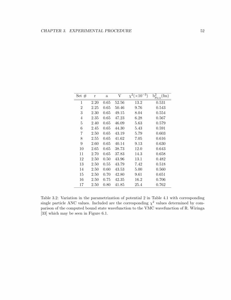
CHAPTER 3. EXPERIMENTAL PROCEDURE 52
Set # r a V χ2(×10−3) b2p3/2
(fm)
1 2.20 0.65 52.56 13.2 0.5312 2.25 0.65 50.46 9.76 0.5433 2.30 0.65 49.15 8.04 0.5544 2.35 0.65 47.23 6.28 0.5675 2.40 0.65 46.09 5.63 0.5796 2.45 0.65 44.30 5.43 0.5917 2.50 0.65 43.19 5.79 0.6038 2.55 0.65 41.62 7.05 0.6169 2.60 0.65 40.14 9.13 0.63010 2.65 0.65 38.73 12.0 0.64311 2.70 0.65 37.83 14.3 0.65812 2.50 0.50 43.96 13.1 0.48213 2.50 0.55 43.79 7.42 0.51814 2.50 0.60 43.53 5.00 0.56015 2.50 0.70 42.80 9.61 0.65116 2.50 0.75 42.35 16.2 0.70617 2.50 0.80 41.85 25.4 0.762
Table 3.2: Variation in the parametrization of potential 2 in Table 4.1 with correspondingsingle particle ANC values. Included are the corresponding χ2 values determined by com-parison of the computed bound state wavefunction to the VMC wavefunction of R. Wiringa[33] which may be seen in Figure 6.1.
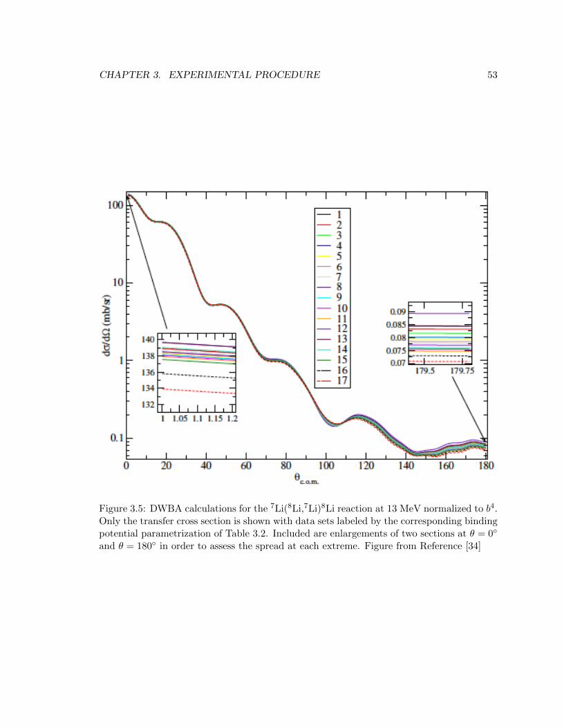
CHAPTER 3. EXPERIMENTAL PROCEDURE 53
Figure 3.5: DWBA calculations for the 7Li(8Li,7Li)8Li reaction at 13 MeV normalized to b4.Only the transfer cross section is shown with data sets labeled by the corresponding bindingpotential parametrization of Table 3.2. Included are enlargements of two sections at θ = 0
and θ = 180 in order to assess the spread at each extreme. Figure from Reference [34]

Chapter 4
Analysis Software
Modern day nuclear physics experiments require sophisticated software for acquiring, sort-
ing, calibrating, reducing and analyzing the data. Many programs are written specifically
to perform a single calculation or task and are generally maintained as needed by a single
user or a small user group. There also exists a large group of software programs that are
developed and widely used across the field. Two of these widely used programs that are used
in this thesis will be discussed in this chapter. The first software program is ROOT, which
is used for calibration and sorting of data collected from the experiment. The second piece
of software is FRESCO and the associated SFRESCO codes used for performing DWBA
calculations and fitting theoretical cross sections to the data. Before discussing those topics
the data acquisition system used will be briefly discussed.
4.1 MIDAS
The TUDA data acquisition system MIDAS is built from a package of software components
and techniques originally developed for Eurogam but is now considerably extended and used
for a wide range of applications. The applications of MIDAS currently include Eurogam,
Euroball, Exogam, Megha, Charissa, GREAT, TIARA and others.
The Midas GUI is based on a script language known as Tcl/Tk. Although Sun originally
sponsored this development, in recent years the package is available on a wide range of
hardware platforms including Sun Solaris and Microsoft Windows. Tcl/Tk has a Motif-like
graphical user interface which makes it fully compatible with the CDE window manager
used on Sun Solaris systems. All documentation and files for MIDAS can be found at
54

CHAPTER 4. ANALYSIS SOFTWARE 55
http://npg.dl.ac.uk/MIDAS/index.html.
4.2 ROOT
ROOT was developed in the context of the NA49 experiment at CERN to handle the large
amount of data produced by the experiment. Around 10 terabytes of data were generated per
run which provided the ideal environment for developers Rene Brun and Fons Rademakers
to develop and test their conceived object oriented design for next generation data analysis.
ROOT was to replace aging FORTRAN libraries that had reached their limits and could
not scale up to the challenges offered by the Large Hadron Collider due to amounts of data
a few orders of magnitude larger than anything seen before [35].
The experiment of this thesis by no means had the large amount of data that ROOT
was originally designed to handle, as data files are on the order of 200 megabytes per run;
however, ROOT still provided an excellent environment for data calibration, sorting events,
and fitting histograms.
ROOT is not a standalone program, it is a data analysis framework. For the command
line and script processor, ROOT uses CINT as its C++ interpreter. Along with ROOT, a
software program called tudaROOT written by Jonty Pearson was used to convert the data
files from the experiment, originally in the MIDAS format, into ROOT data files. For more
details concerning ROOT or for source code please refer to Reference [35].
4.2.1 Framework
Working inside an existing framework eliminates the need to develop tools and code for basic
routines and algorithms. An apt comparison to programming inside a framework is building
a house in a city. In a city there is already infrastructure in place for plumbing, electricity,
and telephone; these are not needed to be developed, merely connected. Building a house in
the country where none of this infrastructure exists and needs to be developed along with
the house is similar to programming outside a framework, where all the infrastructure needs
to be developed along with the program.
Another benefit of working within a framework is that the routines and algorithms in
the framework have already been tested and found accurate and reliable. A drawback of
a framework is that you are constrained to work within its boundaries, which in the case
of the ROOT framework did not pose a problem for the analysis for the experiment of this

CHAPTER 4. ANALYSIS SOFTWARE 56
thesis. The main uses of the ROOT framework here are reduction, calibration and sorting
of data, as well as collecting events into histograms and the fitting of the histograms. Most
of these applications will be discussed in Chapter 5. Before getting to that, I will briefly
touch on ROOT’s handling of histograms.
4.2.2 Histograms
Histograms are a basic component of data analysis in nuclear physics experiments. They
provide a simple method of displaying a large number of events, as well as a visual means
of reducing data by implementing cuts via either kinematics or timing conditions. The his-
togram class in the ROOT framework supports one, two, and three dimensional histograms
with either one byte, short, integer, float, or double values per channel. All histograms
support fixed or variable bin sizes.
Filling a histogram in the ROOT framework is performed by a simple “FILL” command
with a required call value based on the data being collected. The histogram class contains
a “Fill” method which computes the bin number corresponding to the given arguments
and increments the bin. Several other methods exist that perform the functions of adding,
dividing and multiplying histograms together or by a constant value. The ability to easily
create and fill histograms is only one of the many benefits granted by working in the ROOT
framework.
4.2.3 Fitting Histograms
The advantage of using the ROOT framework to fit histograms is evident when fitting
multiple histograms. By using an input file to define predetermined limits, fit results can
quickly be obtained and compared for various kinematic or timing cuts. The framework
also supports fitting multiple peaks in a single range and background estimates.
The minimization package used by ROOT, MINUIT1, originally written in FORTRAN
by Fred James, was converted to a C++ class by Rene Brun. The “MINUIT” package
acts on a multi parameter FORTRAN function to which one must give the generic name
“FCN”. The function “Fit” defines the MINUIT fitting procedure as being being either a
chi-squared or binned likelihood minimization. It is the task of MINUIT to find the values
of the parameters which give the best fit.
1For more information on the MINUIT package see Appendix C
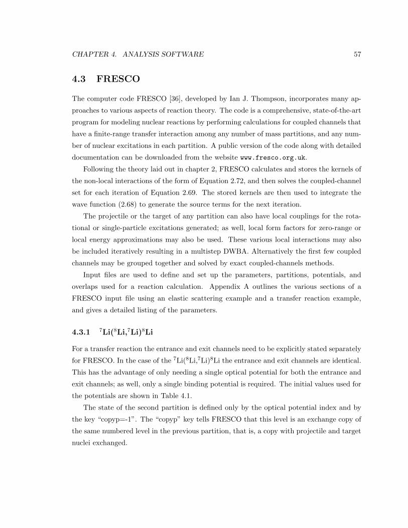
CHAPTER 4. ANALYSIS SOFTWARE 57
4.3 FRESCO
The computer code FRESCO [36], developed by Ian J. Thompson, incorporates many ap-
proaches to various aspects of reaction theory. The code is a comprehensive, state-of-the-art
program for modeling nuclear reactions by performing calculations for coupled channels that
have a finite-range transfer interaction among any number of mass partitions, and any num-
ber of nuclear excitations in each partition. A public version of the code along with detailed
documentation can be downloaded from the website www.fresco.org.uk.
Following the theory laid out in chapter 2, FRESCO calculates and stores the kernels of
the non-local interactions of the form of Equation 2.72, and then solves the coupled-channel
set for each iteration of Equation 2.69. The stored kernels are then used to integrate the
wave function (2.68) to generate the source terms for the next iteration.
The projectile or the target of any partition can also have local couplings for the rota-
tional or single-particle excitations generated; as well, local form factors for zero-range or
local energy approximations may also be used. These various local interactions may also
be included iteratively resulting in a multistep DWBA. Alternatively the first few coupled
channels may be grouped together and solved by exact coupled-channels methods.
Input files are used to define and set up the parameters, partitions, potentials, and
overlaps used for a reaction calculation. Appendix A outlines the various sections of a
FRESCO input file using an elastic scattering example and a transfer reaction example,
and gives a detailed listing of the parameters.
4.3.1 7Li(8Li,7Li)8Li
For a transfer reaction the entrance and exit channels need to be explicitly stated separately
for FRESCO. In the case of the 7Li(8Li,7Li)8Li the entrance and exit channels are identical.
This has the advantage of only needing a single optical potential for both the entrance and
exit channels; as well, only a single binding potential is required. The initial values used for
the potentials are shown in Table 4.1.
The state of the second partition is defined only by the optical potential index and by
the key “copyp=-1”. The “copyp” key tells FRESCO that this level is an exchange copy of
the same numbered level in the previous partition, that is, a copy with projectile and target
nuclei exchanged.

CHAPTER 4. ANALYSIS SOFTWARE 58
kp Interaction V VSO rV aV WV rW aW rC Ref.
1 7Li + 8Li 175 0.64 0.8 16.9 1.09 0.8 1.3 [34]2 (n + 7Li)p3/2
43.19 0.0 2.5 0.65 2.5 [38]
4 (n + 7Li)p1/242.14 4.9 2.391 0.520 2.391 [39]
10 7Li + 7Li 4.66 0.173 1.617 5.60 1.589 0.397 1.3 [40]
Table 4.1: Interaction potentials used for FRESCO calculation of 7Li(8Li,7Li)8Li reactionat 11 MeV. The “kp” value corresponds to the index of the potential as it appears in theinput file of Figure B.3. Real and imaginary depths, V and W, are expressed in MeV.Radii and diffusenesses are in fm. The radii of the optical potentials are reduced, and full
radii follow the convention Ri = ri(A1/3t +A
1/3p ) where i is either V or W. Potential 1 is
the optical potential for the interaction between the 7Li + 8Li nuclei. Potentials 2 and 4are binding potentials for the p3/2 and p1/2 orbitals respectively, and potential 10 is thecore-core interaction.
With no optical potential for the 8Li+7Li reaction at 11 MeV to be found in the litera-
ture, the initial optical potential used is taken from Reference [34]. The parameters of this
potential are derived from systematic studies of 8Li elastic scattering data at laboratory
energies from 13 to 20 MeV with targets in the mass range of 1 to 58 amu [41]. Separate
binding potentials are needed for both the p3/2 and p1/2 states for the valence neutron in 8Li.
The p3/2 binding potential is taken from Reference [38], while the p1/2 binding potential is
taken from Reference [39]. The core-core potential is a volume-dominated optical potential
for the interaction between 7Li and 7Li taken from a study at laboratory energies from 5 to
40 MeV [40].
The overlap and coupling is also simplified due to the symmetry of the reaction and only
requires the overlap for the valence neutron on 7Li. The spectroscopic amplitude, however,
must appear twice, once for each vertex in the reaction. The initial values for the p3/2
and p1/2 spectroscopic amplitudes are set to the values from Reference [33]. During the
fitting process the p3/2 spectroscopic amplitude is allowed to vary while the p1/2 amplitude
remains fixed at the initial value. Due to the requirement of each amplitude to appear in
the FRESCO input file twice, the actual value of the spectroscopic factor for each orbital
is given by the product of the amplitudes for the entrance and exit channels [42]. With
the reduced amount of usable data collected during the experiment the number of degrees
of freedom to fit for both spectroscopic amplitudes would have significantly reduced the
quality of or even limited the possibility of obtaining a convergent fit. Lacking the angular

CHAPTER 4. ANALYSIS SOFTWARE 59
coverage to separately determine both the p1/2 and p3/2 spectroscopic amplitudes the p1/2
spectroscopic amplitude is held fixed. This is discussed further in Section 5.3
This input file provides a starting place for fitting theoretical calculations to the data.
Initial fits are performed to adjust the entrance and exit optical potential by fixing the
spectroscopic amplitudes at currently accepted values and allowing only the optical potential
parameters to vary. Once a χ2 minimization is reached for the optical potential, the resulting
values are substituted in as starting values for a new minimization where the optical potential
for the entrance and exit channels as well as the p3/2 spectroscopic amplitude are fit. Full
details of the analysis and results from the SFRESCO fit can be found in section 5.3.
4.4 SFRESCO
A first calculation of the cross section using FRESCO will often produce results that differ
from experimental data. Whether the reaction model is too simplified or the input parame-
ters are not accurate enough the FRESCO calculation may be improved upon by using the
program SFRESCO, the Search version of FRESCO. SFRESCO uses the MINUIT routines
to search for a χ2 minimum when comparing the outputs of FRESCO with datasets.
Along with a standard input file as described in section 4.3, an input file for SFRESCO
and a SFRESCO script are required to perform a SFRESCO minimization. The input file
specifies the FRESCO input and output files, the number and types of the search variable,
and the experimental data sets to be compared against. The script is a simple method of
entering commands to SFRESCO to perform the fit as desired; alternatively the commands
may be entered manually via the command line. As a simple example of a SFRESCO
minimization, an elastic scattering example of a proton scattering off of 112Cd is provided
below.
4.4.1 p + 112Cd elastic scattering
The following example is from the FRESCO User’s Guide which may be found at the
website www.fresco.org.uk. A basic input file (Figure B.4) for FRESCO is required that
defines the energy, partitions, states, and the potentials needed for the calculation. The
potential is defined here using the “type” variable which indicates the shape of the potential.
Type 0 is for Coulomb potentials, type 1 for volume central potentials, type 2 for surface

CHAPTER 4. ANALYSIS SOFTWARE 60
central potentials, type 3 for spin-orbit potentials for the projectile, and type 4 for spin-orbit
potentials for the target.
The SFRESCO input file shown in Figure B.6 begins with the filename of the FRESCO
input file and the desired output filename. The following line indicates the number of pa-
rameters to be fit followed by the number of experimental datasets. The header “&variable”
lists the parameters to vary during the minimization. In this example all the parameters are
variables of the interaction potential and are of the type “kind=1”. The individual variables
are identified by the values of: “kp”, the index of the potential, “pline”, the line within the
potential, and “col”, the column number for the given line. The optional “potential” value
is used to override the default values given in the FRESCO input file. A final “step” value
sets the initial magnitude for trial changes. Other optional values not included are minimum
and maximum values for the parameter, “valmin” and “valmax”, respectively.
Type Description
0 Angular distribution for fixed energy1 Excitation and angular cross-section double distributions2 Excitation cross section for fixed angle3 Excitation function for the total, reaction, fusion, or inelastic cross section4 Excitation phase shift for fixed partial wave5 Desired factor for bound-state search6 Specific experimental constraint on some search parameter.
Table 4.2: SFRESCO data types
Experimental datasets are identified by their “type”. A list of the different types available
are summarized in Table 4.2. A data file may be used to input the dataset by entering a
filename, or the data can be listed in the input file by replacing the filename with “data”
as is done in this example. A value may be supplied for the number of data points to read
in; if a value is not supplied all the listed data are used. The value of “iscale” indicates the
units of the data and is -1 for relative data, 0 for absolute data in units of fm2/sr, 1 for
b/sr, 2 for mb/sr, and 3 for µb/sr. To indicate the desired format for the output, “idir” is
set to -1 for cross section data given as astrophysical S factors, 0 for data given in absolute
units, and 1 as a ratio to Rutherford. The reference frame for which the dataset is given is
indicated by the value of the input parameter “lab” and is “T” or “F” for laboratory angles
and cross sections. Finally, if “abserr” is true, the third column of the dataset is treated as

CHAPTER 4. ANALYSIS SOFTWARE 61
absolute errors.
1.2
1.0
0.8
0.6
0.4
0.2
0.0
σ/σ
R
18016014012010080604020
Center of Mass Scattering Angle (degrees)
Experimental data
Fitted parameters Initial parameters
Figure 4.1: Data and calculations of proton scattering on 112Cd at 27.90 MeV with initialand fitted potential parameters.
SFRESCO may be run using an input script, as shown in Figure B.5, or by directly
interacting with the command line. When multiple minimizations are required or the run
time is long a script proves useful. A minimum set of commands is required and includes: the
SFRESCO input filename, “min”, “migrad”, “end”, and “plot”. The “min” command calls
MINUIT interactively using the starting values and variables defined in the SFRESCO input
file. This is followed by “migrad” which within MINUIT performs a MIGRAD2 search. The
“end” command returns to SFRESCO from MINUIT, the “plot” command is not required
for a minimization; its function is to produce a file with the data and theory curves for
display with the program xmgr, a 2d plotting tool. Many more commands are available and
a full list may be found in appendix A.
2For more information on MINUIT and the MIGRAD minimizer please refer to Appendix C

CHAPTER 4. ANALYSIS SOFTWARE 62
Parameter Initial Value Final Value
V 45.5 MeV 52.18 MeVW 1.5 MeV 2.90 MeV
WD 4.5 MeV 8.18 MeVr0 1.17 fm 1.18 fm
Table 4.3: SFRESCO fit results for p + 112Cd elastic scattering from input files displayedin Figures B.4 and B.6
The results of the SFRESCO minimization from the input of Figures B.4 and B.6 are
displayed in Figure 4.1. The initial FRESCO calculation is shown as well as the final
FRESCO calculation using the final values for the parameters that were varied. The fitted
parameters are displayed in Table 4.3.
4.4.2 Minuit Error
From SFRESCO, the solution of a minimization problem using Minuit is itself straightfor-
ward. The calculation or interpretation of the resulting parameter uncertainties is consider-
ably more complicated. Specific complications for this fit arise from multi-parameter error
definition and interpretation. With more than one free parameter problems may arise in
interpreting errors from Minuit. The output from Minuit gives an error matrix from which
the individual parameter error values are calculated.
The error matrix, also called the covariance matrix, is the inverse of the matrix of
second derivatives. The diagonal elements of the error matrix are the variances (squares
of the standard deviations) of the corresponding parameters, and the off-diagonal elements
indicate the degree of correlation, positive or negative, between the corresponding pairs
of parameters [43]. Calculations of the error in this fashion take into account effects of
correlations among parameters.
In order to ensure accurate error values from the fitting procedure an extra call was made
to Minuit instructing it to calculate the Hessian matrix. The call calculates the full matrix
of second derivatives of the function with respect to the currently variable parameters, and
inverts it, printing out the resulting error matrix.

Chapter 5
Data Analysis
Progressing from a collection of signals in various ADCs, and TDCs to a final result requires
many different stages of data processing and analysis. The next two chapters discuss details
of the data reduction and analysis, as well as the fitting of theory to the results of the
experiment.
5.1 Detector Calibration
The first step before performing data reduction is to perform energy and time calibrations for
the detectors and associated electronics. This ensures that all detected events are properly
adjusted for variations between the separate elements. Specific problems with detector
readouts may also need to be identified and addressed. Other steps involving the physical
properties of the detectors ranging from actual position relative to the beam spot and
amount of active area present in an azimuthal range need to be calculated and corrected.
Once all this initial calibration is complete, the data extraction and subsequent analysis can
commence. Applying gates on the energy and time spectra to select areas of interest can
reduce background and aid in identifying loci, eventually leading to a final reduction of the
data for fitting. After removing as much background as possible and applying appropriate
adjustments and corrections, the theory can be fit to data to obtain the final results.
63

CHAPTER 5. DATA ANALYSIS 64
5.1.1 Energy and Time calibration
As was discussed in Chapter 3, the detectors were calibrated before the experiment and
immediately following it using a triple–α source. The α peaks are fit with gaussian functions,
resulting in a centroid channel number for each energy peak in each ADC. These centroid
channel numbers are then fit with a linear function to reproduce the known energies of the
α’s corrected for energy loss from SRIM calculations [44]. The energy calibration for each
ADC channel consists of an offset and a gain variable.
The TDCs were calibrated using a pulser prior to the commencement of the run. The
pulse generator was connected to all TDC channels. The result is a readout where all
channels are triggered with a simultaneous event. From this pulser data the individual
TDC channels were calibrated by applying an offset value to raw data during analysis. The
calibrated data from the TDC shows a uniform time from the pulser whereas before the
calibration slight variations on the timing were present due to variations in the individual
electronics of each channel.
5.1.2 Beam Offset
The presence of 19F in the target resulted in elastic scattering which could be analyzed for
detector calibration. Comparing the absolute numbers of scattered 8Li among the sectors
detected in the S2 detector between laboratory angles of 5 to 15 degrees an asymmetry
shown in Figure 5.1, is observed. This asymmetry arises from a slight displacement of the
beam spot from the center of the detectors.
The calculated angular range for the recoil and ejectile from the 7Li(8Li,7Li)8Li reaction
can be seen in Table 5.1. The LEDA detector covers a range from 36 to 60 degrees in the
laboratory frame. For a coincidence event in this range one particle is detected at the lower
range of accepted angles by the LEDA detector, while the other event is detected near the
middle of the detector’s range. This fact aided in the confirmation of the beam offset. Due
to the beam offset the angular coverage of each sector in the detector is shifted. Sectors that
are closer to the beam axis have an angular range that is shifted down, while sectors on the
opposite side of the detector where the beam axis is shifted away from the sector result in
an upward shift in the angular range. Comparing these coincidence events an asymmetry
is also observed. Although the effect is much smaller in the LEDA than in the S2 due to
the differences between the angular size of each detector, this asymmetry observed in both

CHAPTER 5. DATA ANALYSIS 65
20x103
15
10
5
0
Inte
gra
ted C
ounts
75070065060055050045040035030025020015010050
S2 Channel Number
Figure 5.1: Elastic scattering of 8Li from 19F. The x-axis represents the S2 channel numberstarting at x=0 for sector 0 ring 0 and incrementing by ring (i.e. x=1 represents sector 0ring 1, x=2 represents sector 0 ring 2). Each sector consists of 48 rings and there are a totalof 16 sectors.

CHAPTER 5. DATA ANALYSIS 66
detectors indicates a beam offset from the detector centers.
Ejectile angle () Recoil angle ()
35 49.5238 47.0941 44.5844 42.0247 39.4150 36.7753 34.0956 31.4059 28.68
Table 5.1: Kinematically calculated range of the recoil and ejectile angles in degrees fromthe 7Li(8Li,7Li)8Li reaction. The LEDA detector covers a range from 36 to 60 degrees.
Using the data from 19F elastically scattered events a minimization was performed to
determine the offset of each detector from the beam axis. By varying the offset values and
thus the correlated scattering angle the asymmetry is minimized and the beam offset is
determined.
S2 offsetRun Group x (±0.001) (cm) y (±0.001) (cm)
1 0.061 0.1442 0.058 0.1433 0.082 0.1194 0.023 0.117
Table 5.2: Calculated beam offset based on asymmetry of elastically scattered 19F events
On account of the superior angular resolution due to segmentation in the S2 detector as
well as significantly higher event counts, the offset for the S2 detector introduces a larger
effect than the offset for the LEDA detector. Due to the larger spacing of the rings the
effect of the offset was found to be negligible in the LEDA detector. The offset values from
the minimization from the S2 data are displayed in Table 5.1.2 in units of centimeters. The
multiple entries for the offset correspond to groupings of run files from the experiment. Each
significant change to the offset is correlated with a logged change in the beam tune during

CHAPTER 5. DATA ANALYSIS 67
the experiment. Since the effect of the offset on the data from the LEDA detector was
negligible no offset was used for the data from the LEDA.
5.1.3 Detector Geometry
Corrections for the amount of active area present in a given angular range due to inactive
areas of the detectors, as well as the effects of the offset between the beam spot and the
detector centers, are accounted for via Monte Carlo simulations. A program was written to
evaluate the fraction of events striking the active area of each detector segment as a function
of laboratory angle.
The Monte Carlo program generates a large number of events with a random scattering
angle within a preset range. Each event is then compared to the detector geometry and
it is determined whether it impacted a region of active area on the detector and is thus
considered a good hit, or impacted a dead region and is counted as a miss. The detector
efficiency for a given angular range is calculated as the number of good hits in that angular
range divided by the total number of events simulated.
For the S2 detector the width of each bin is set to 1.0 degree and a total of 5 × 10⁷
events are generated in each bin. The LEDA detector was simulated with bin sizes ranging
from 1.6 to 2.5 corresponding to the distinct rings in the detector. As well as the primary
event the LEDA also required the simulation of a second event on the opposite side of the
detector within a range corresponding to the coincident recoil. The number of primary
events generated for the LEDA detector was 107 with each primary generating a single
coincident recoil event.
The resulting geometric coverage of each 1 (laboratory angle) bin in the S2 detector
ranged from 12% for bins on the edge of the detector to 78%. The decision to use 1 bin
sizing in the S2 detector rather then the natural bin size from the individual rings of the
detector was due to the effect of the offset. Due to the small size of the rings the offset
created large shifts in the scattering angle between opposite sides of a single ring. By using
a much larger bin size than the physical size of a ring, binning errors introduced from the
offset are reduced. This choice to use large bin sizes in the S2 detector was also due to
the lack of coincident recoils and resulting difficulty separating the data from background
events. The high statistics in a given bin provided a reliable means for precise data reduction
through the multiple peak fitting procedure discussed in section 5.2.3.
The geometric efficiency of the S2 as a function of scattering angle varies over a large
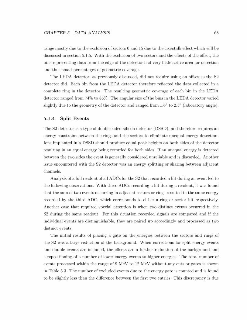
CHAPTER 5. DATA ANALYSIS 68
range mostly due to the exclusion of sectors 0 and 15 due to the crosstalk effect which will be
discussed in section 5.1.5. With the exclusion of two sectors and the effects of the offset, the
bins representing data from the edge of the detector had very little active area for detection
and thus small percentages of geometric coverage.
The LEDA detector, as previously discussed, did not require using an offset as the S2
detector did. Each bin from the LEDA detector therefore reflected the data collected in a
complete ring in the detector. The resulting geometric coverage of each bin in the LEDA
detector ranged from 74% to 85%. The angular size of the bins in the LEDA detector varied
slightly due to the geometry of the detector and ranged from 1.6 to 2.5 (laboratory angle).
5.1.4 Split Events
The S2 detector is a type of double sided silicon detector (DSSD), and therefore requires an
energy constraint between the rings and the sectors to eliminate unequal energy detection.
Ions implanted in a DSSD should produce equal peak heights on both sides of the detector
resulting in an equal energy being recorded for both sides. If an unequal energy is detected
between the two sides the event is generally considered unreliable and is discarded. Another
issue encountered with the S2 detector was an energy splitting or sharing between adjacent
channels.
Analysis of a full readout of all ADCs for the S2 that recorded a hit during an event led to
the following observations. With three ADCs recording a hit during a readout, it was found
that the sum of two events occurring in adjacent sectors or rings resulted in the same energy
recorded by the third ADC, which corresponds to either a ring or sector hit respectively.
Another case that required special attention is when two distinct events occurred in the
S2 during the same readout. For this situation recorded signals are compared and if the
individual events are distinguishable, they are paired up accordingly and processed as two
distinct events.
The initial results of placing a gate on the energies between the sectors and rings of
the S2 was a large reduction of the background. When corrections for split energy events
and double events are included, the effects are a further reduction of the background and
a repositioning of a number of lower energy events to higher energies. The total number of
events processed within the range of 9 MeV to 12 MeV without any cuts or gates is shown
in Table 5.3. The number of excluded events due to the energy gate is counted and is found
to be slightly less than the difference between the first two entries. This discrepancy is due

CHAPTER 5. DATA ANALYSIS 69
Range Number of Events
9 - 12 MeV 7.90× 10⁷
Equal Energy Gate 6.27× 10⁷
Omitted 1.55× 10⁷
Equal Energy + corrections 6.61× 10⁷
Table 5.3: Total number of events processed in the S2 detector prior to and following theapplication of energy gates to the data. The final entry includes all events after equal energygates and corrections to events discussed due to energy splitting between adjacent channels.
to a double counting effect in the un-gated range from split energy events. The final entry in
Table 5.3 includes the corrections from the energy gate as well as from split energy events.
It is slightly greater than the number of events processed with only the energy gate due to
the inclusion of events that are excluded by the 9 to 12 MeV energy window due to energy
splitting effects previously discussed.
Two dimensional histograms depicting the events detected in the S2 detector between
9 and 12 MeV are displayed in Figure 5.2. The top left panel represents the first entry in
Table 5.3. The top right panel shows the events remaining after removing all events that
did not have equal energies within 3% between the sectors and rings of the detector. In
the bottom left panel the events omitted between the top two panels are displayed, and the
final panel shows the events after the energy gate and corrections for split energy events are
included.
5.1.5 S2 Crosstalk
During the first stages of sorting the collected data from the S2 detector a peculiarity was
noticed in the two sectors located immediately adjacent to the pinout region, where signals
emerge on the detector. These sectors (sector 0 and sector 15) show an oscillatory pattern
overlaid on top of the expected 1sin4(θ/2)
function for elastically scattered 8Li events from a
19F nucleus. The top panel of Figure 5.3 shows the elastically scattered events from the 19F
nuclei for sectors 0 and 15. The bottom panel depicts the expected and typical results for
an elastic scattering spectrum which is observed in all other sectors.
The two sectors 0 and 15 are different from the other sectors since they are adjacent to
the edge of the detector in terms of azimuthal angle and the tracks over the silicon wafer to

CHAPTER 5. DATA ANALYSIS 70
Lab Angle (degrees)6 8 10 12 14
Energ
y (
keV
)
9000
9500
10000
10500
11000
11500
12000
Entries 7.902168e+07Entries 7.902168e+07
1
10
210
310
410
Energy vs Scattering Angle
Lab Angle (degrees)6 8 10 12 14
Energ
y (
keV
)
9000
9500
10000
10500
11000
11500
12000
Entries 6.267803e+07Entries 6.267803e+07
1
10
210
310
410
Energy vs Scattering Angle
Lab Angle (degrees)6 8 10 12 14
Energ
y (
keV
)
9000
9500
10000
10500
11000
11500
12000
Entries 1.552979e+07Entries 1.552979e+07
1
10
210
310
Energy vs Scattering Angle
Lab Angle (degrees)6 8 10 12 14
En
erg
y (
ke
V)
9000
9500
10000
10500
11000
11500
12000
Entries 6.611961e+07Entries 6.611961e+07
1
10
210
310
410
Energy vs Scattering Angle
Figure 5.2: Top Left: All events in the S2 with energy detected in a ring between 9 and 12MeV. Top Right: Events in the S2 with a 3% agreement between ring and sector energy.Bottom Left: Events excluded between top two histograms. Bottom Right: All eventsbetween 9 and 12 MeV with equal energy and corrections for events with split energy.

CHAPTER 5. DATA ANALYSIS 71
Figure 5.3: Top panel shows the cross talk observed in sectors 0 and 15 in the S2 detectorcreating an oscillatory output. Bottom panel shows the observed output for elastic scatteringfrom sector 1. Similar output is observed in all other sectors as well. Both figures show 8Lielastically scattered from 19F as a function of S2 ring number.

CHAPTER 5. DATA ANALYSIS 72
the inner strips. The suspected cause of the problem is a type of crosstalk or inter-strip effect
(i.e. a hit somewhere other than the active area defined by the p+ and n+ implantation)
[45]. Requiring equal energies in the sectors and rings of the S2 detector was tested as a
solution to the observed crosstalk effect. However, even with a stringent requirement of a
1% agreement between energies from the two sides of the detector, the oscillatory behavior
was still observed.
Figure 5.4: S2 detector mounted in the TUDA chamber.
After further investigation of the matter without discovering a concrete solution, it was

CHAPTER 5. DATA ANALYSIS 73
decided to omit the events from sectors 0 and 15 in the S2 detector. These two sectors
amount to under 1/8 of the active area of the detector. The exclusion of the two sectors
is only a minor problem, as the statistics at the small scattering angles covered by the S2
detector are quite sufficient even with the omitted events.
5.2 Data Reduction
Following implementation of the corrections and techniques discussed in the previous sec-
tions of this chapter, the spectra are analyzed and further refinements are made by imposing
energy and timing cuts. Optimizing the cuts and the gates on the data, the background is
reduced while accepting as many good events as possible. Identifying the remaining back-
ground peaks helps when applying multiple peak fits to the data in the S2 detector. By
performing a multiple peak fit the data in the S2 can be extracted even though a recoil
coincident event with the LEDA detector was not available.
5.2.1 Background Reduction
With previous background reduction and corrections applied, the data from the S2 detector
is further constrained by energy and time cuts. Previous energy gates between the rings and
sectors in the S2 detector as discussed in section 5.1.4 ensure that the energy deposited in
the rings and sectors agrees within 3%. This value is used as a rough initial cut to remove
most background events in the S2. A further refinement by means of a manually created
gate results in the sector energy vs. ring energy cut shown in Figure 5.5.
Timing data is also used to gate on the loci of interest and reduce background events.
Identification of various peaks in the TDC data was done by placing tight windows on known
loci in the energy spectrum and assessing the corresponding peak in the timing data. A
timing window is placed between channels 306 and 328 on the ring channels and between
channels 310 and 328 on the sector channels. When both the refined energy cut and the
timing cut are applied, the energy-angle data from the S2 detector appear in Figure 5.7.
TDC spectra for the S2 detector are shown in Figure 5.6. The spectra include full TDC
data before any energy or timing cuts are made for both the sectors and the rings as well
as the comparison following the implementation of energy and timing cuts.
Data from the LEDA detector were easily reduced by using coincidences to separate
events of interest from background. The kinematics of the 7Li(8Li,7Li)8Li reaction are such

CHAPTER 5. DATA ANALYSIS 74
Figure 5.5: Sector energy vs. ring energy cut in the S2 detector.

CHAPTER 5. DATA ANALYSIS 75
Entries 5.798843e+07
240 250 260 270 280 290 300 310 320 330
310
410
510
610
710
Entries 5.798843e+07TDC004 valS2 Sector TDC
Channel
Cou
nt
Entries 7700769
240 250 260 270 280 290 300 310 320 330
310
410
510
Entries 7700769TDC006 valS2 Sector TDC Remaining
Channel
Cou
nt
Entries 5.798843e+07
240 250 260 270 280 290 300 310 320 330
410
510
610
Entries 5.798843e+07TDC003 valS2 Ring TDC
Channel
Cou
nt
Entries 7700769
240 250 260 270 280 290 300 310 320 330
410
510
Entries 7700769TDC005 valS2 Ring TDC Remaining
Channel
Cou
nt
Figure 5.6: TDC spectrum from the S2 detector. The top two figures are the TDC datafrom the sectors while the bottom two are from the rings. The figures on the left hand siderepresent the full uncut TDC data for either the sectors or the rings. On the right handside are the excluded events after energy and timing cuts are made.

CHAPTER 5. DATA ANALYSIS 76
Lab Angle (degrees)6 8 10 12 14
En
erg
y (
ke
V)
9000
9500
10000
10500
11000
11500
12000
Entries 5.404774e+07Entries 5.404774e+07
1
10
210
310
410
Energy vs Scattering Angle
Figure 5.7: Two dimensional laboratory energy vs. angle histogram depicting the S2 datawith all energy and time cuts applied. Identification of the various loci is shown in Figure5.9. The two faint loci above the beam energy of 11 MeV located around 12 MeV and 11.5MeV are from the positive Q value reaction of the neutron transfer between 8Li and 12C tothe ground state and the first excited state of lithium, 12C(8Li,7Li)13C and 12C(8Li,7Li∗)13Crespectively.
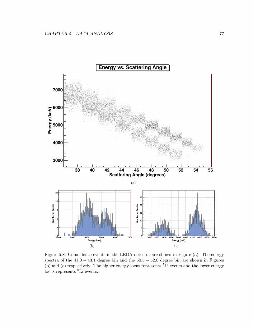
CHAPTER 5. DATA ANALYSIS 77
Scattering Angle (degrees)38 40 42 44 46 48 50 52 54 56
En
erg
y (
ke
V)
3000
4000
5000
6000
7000
hEvsTheta5vEntries 2983
Mean x 44.6
Mean y 5270RMS x 4.844
RMS y 998.7
hEvsTheta5vEntries 2983
Mean x 44.6
Mean y 5270RMS x 4.844
RMS y 998.7Energy vs. Scattering Angle
(a)hEvsTheta5v_py
Entries 3025
Mean 5740
RMS 381.3
Energy (keV)
4500 5000 5500 6000 6500 7000
Nu
mb
er
of
En
trie
s
0
5
10
15
20
25
hEvsTheta5v_py
Entries 3025
Mean 5740
RMS 381.3ProjectionY of binx=3
(b)
hEvsTheta5v_py
Entries 1664
Mean 3983
RMS 471.7
Energy (keV)
3000 3200 3400 3600 3800 4000 4200 4400 4600 4800
Nu
mb
er
of
En
trie
s
0
5
10
15
20
25
hEvsTheta5v_py
Entries 1664
Mean 3983
RMS 471.7ProjectionY of binx=8
(c)
Figure 5.8: Coincidence events in the LEDA detector are shown in Figure (a). The energyspectra of the 41.0 − 43.1 degree bin and the 50.5 − 52.0 degree bin are shown in Figures(b) and (c) respectively. The higher energy locus represents 7Li events and the lower energylocus represents 8Li events.

CHAPTER 5. DATA ANALYSIS 78
that the angular range of both the recoil and the ejectile fall within the range of the LEDA
detector. When placing the energy cuts care was taken to ensure events were not double
counted. Following the detection of an event inside the 8Li window and coincidence event
inside the 7Li window, the individual energies are summed and compared to an acceptance
gate on their total energy. The total energy gate is corrected for energy loss through the
target and dead layer of the LEDA detector based on energy loss calculations from SRIM
[44]. Energy loss through the target is on the order of 80 keV, while energy loss through
the dead layer of the LEDA ranged from 130 keV to 180 keV. Longitudinal and lateral
straggling were also calculated and found to be on the order of 2.03 and 1.25 respectively
through the target and 2.16 and 1.57 respectively in the detectors for 8Li at 11 MeV.
Figure 5.8 shows the detected coincidences of 7Li and 8Li in the LEDA detector. The
top panel depicts the data at a scattering angle of 39 degrees and the bottom panel at a
scattering angle of 49 degrees. The 7Li events are located at a higher energy than the 8Li
events at a given angle. Due to the coincidence requirement and the total energy gate the
background in the LEDA is effectively reduced to zero.
5.2.2 S2 data reduction
Initial plans for data analysis were for the 8Li events in the S2 detector to be separated out
from the large number of background events due to elastic scattering through coincidences
with 7Li in the LEDA detector. The kinematics of the 7Li(8Li,7Li)8Li reaction are such that
when the 8Li recoil is incident within the angular range of the S2, then the low energy 7Li
recoil would fall within the angular range of the LEDA detector. As previously mentioned,
this did not happen because no LEDA events at low energy were recorded.
This abnormally high cutoff energy in the LEDA detectors could originate from one of
two scenarios; either the cutoff value was set in post processing software or in the hardware.
Following the discovery of the missing coincidence, all software programs were checked to
ensure the low energy coincidence events from the LEDA were not being removed in data
processing. After no artificially introduced cutoff value was discovered in the software, the
conclusion that it was a low threshold for the Silena 9418/6V ADCs was reached. Typical
thresholds for the ADC for a TUDA experiment omit the lowest 48 channels [45], however
it appears that somehow all events in the lowest 128 channels of the ADC were discarded
resulting in the coincidence events being discarded. The cause for the abnormally high
thresholds is unknown, but appeared to be a default setting of a previous experiment [45].

CHAPTER 5. DATA ANALYSIS 79
Laboratory Angle (degrees)5 6 7 8 9 10 11 12 13 14
En
erg
y (
ke
V)
9200
9400
9600
9800
10000
10200
10400
10600
10800
11000
hEvsThetaEntries 4.166598e+07
Mean x 7.863
Mean y 1.079e+04
RMS x 2.296
RMS y 153.2
hEvsThetaEntries 4.166598e+07
Mean x 7.863
Mean y 1.079e+04
RMS x 2.296
RMS y 153.2
10
210
310
410
Energy vs Scattering Angle
Energy vs. Scattering Angle
19F(8Li,8Li)19F
12C(8Li,8Li)12C
7Li(8Li,7Li)8Li
7Li(8Li,8Li)7Li7Li(8Li,7Li*)8Li
12C(8Li,8Li*)12C
7Li(8Li,8Li*)7Li1H(8Li,7Li)2H
1H(8Li,8Li)1H
Figure 5.9: Two dimensional histogram of data from the S2 detector after final cuts withidentified loci. No evidence for the loci representing the 19F(8Li,8Li∗)19F, 19F(8Li,7Li)20F,7Li(8Li,8Li)7Li∗, and the 7Li(8Li,7Li)8Li∗ reactions were evident above the background.

CHAPTER 5. DATA ANALYSIS 80
While these coincidence events were missed, the data from the S2 detector are not
completely lost. With the extensive background reduction and tight cuts placed on the data
as previously discussed, the lithium events are separable in a limited range. In Figures 5.7
and 5.9 the 8Li and 7Li elastic scattering locus can be seen separated from the background
due to elastic scattering off of carbon and fluorine above 12 degrees.
5.2.3 Fitting the S2 data
Without the coincidences to separate the 8Li and 7Li elastic scattering locus from the
background, a multiple peak fit for the S2 data is required. Even though the S2 detector
collected data between 4.7 and 15.7 degrees in the laboratory frame, the kinematics of
the reactions made separating the lithium locus from the larger carbon and fluorine loci
impossible at angles below 9 degrees. From 9 degrees and up the lithium peak is sufficiently
separated from the background to perform a reliable multiple peak fit.
The full multi-peak fit includes: a linear background, three gaussians for 8Li scattered
from lithium, carbon, and fluorine respectively, and a fourth gaussian for a background
peak. The fourth gaussian describes a small peak with a nearly uniform energy profile over
the entire angular range which we attribute to elastic scattering from heavy contaminants;
Fe, Te, Ba, and Pb were all known to be present in the target at trace levels. The tail of this
locus is visible in Figure 5.7 around an energy of 10.8 MeV above the fluorine elastic locus .
Performing the fit while excluding this background gaussian resulted in a poor overall fit to
the data; however, the resulting values for the amplitude of the lithium peak are similar to
the fits with the background gaussian included. The average change in the integral of the
lithium peak was a reduction of 1% when including the background peak.
Constraints placed on the fitting parameters for the multiple peak fit were left fairly
loose. The individual widths of the gaussians are required to be within 50% of each other,
while the mean values of the fits are required to be within 5% of the calculated values taking
into account kinematics and energy loss calculations.
A typical multiple peak fit for the S2 data is shown in Figure 5.10. In green is the
elastic lithium peak, and in red is the total fit. The black peaks are elastic scattering from
carbon, fluorine and trace heavy contaminants. The small peaks located around 9.6 MeV
and 9.9 MeV, which are not shown in Figure 5.10 but are visible in Figure 5.9, are inelastic
scattering to the first excited state in 8Li and 7Li. The peak at 9.6 MeV is the 8Li from
inelastic scattering to the first excited state of 8Li at 0.98 MeV from carbon. The peak at 9.9

CHAPTER 5. DATA ANALYSIS 81
Entries 1472727
Energy (keV)10100 10200 10300 10400 10500 10600 10700 10800 10900
Num
ber
of E
vents
210
310
410
510
Entries 1472727Li Integral = 734158 +/ 5414 for 11MeV_xy.root
Li Exchange
Carbon
Fluorine
Heavy Contaminants
Figure 5.10: Data from the S2 detector between 12 and 13 degrees in the laboratory frame.The green curve represents 8Li and 7Li particles from the 7Li + 8Li reaction. The blackcurves are elastic scattering from carbon, elastic scattering from fluorine, and a backgroundpeak that is nearly uniform across all angles in the S2 detector at the beam energy attributedto elastic scattering from trace heavy contaminants. The red curve is the sum of the fourgaussians and the linear background.

CHAPTER 5. DATA ANALYSIS 82
MeV is attributed to 8Li from inelastic scattering to the first excited state in 7Li at 0.48 MeV
from the 7Li(8Li,7Li)8Li reaction. Due to the small size of these peaks their contributions
are included in a linear background. Also approximated as a part of the linear background
is the small peak located above the beam energy around 11.3 MeV, also not shown in Figure
5.10 but visible in Figure 5.9, which is the result of scattering to the first excited state of
7Li in the neutron transfer reaction with carbon. The small peaks are omitted from view in
Figure 5.10 to show the details in a narrower range around the peaks of interest. The small
excess of events above the fit at the low energy tail of the “Li Exchange” peak amounts to
only 0.37% of the total 8Li and 7Li events from the 7Li(8Li,7Li)8Li reaction deduced from
the fit.
5.2.4 Error estimates
The errors assigned to the reduced data from the S2 and LEDA detectors are the results of
multiple sources. As each detector requires unique data analysis methods, their sources of
errors will be discussed separately.
For the S2 detector the large number of events resulted in small statistical error values.
Typical statistical errors from the gaussian fits are on the order of ±1.5% or less. The
largest sources of error for the S2 data are due to systematics. These errors arise from
the extensive measures required to reduce the background and the difficulty in accurately
performing multiple peak fits. The similar timing and energy of 8Li nuclei scattered at small
angles from either 19F or 7Li enabled the use of the 19F peak to estimate the systematic error
due background reduction cuts and fitting. By comparing the peaks for the 19F scattering
before and after implementing background reduction an estimated error of ±5% due to the
energy and time gates placed on the S2 data is estimated. The final source of error for
the S2 detector arises from a variation in the determined beam offset position. Varying the
offset by 0.10 cm in all directions and comparing the results, a systematic error of ±4.7%
from the beam offset applies to the S2 data.
The errors for the data from the LEDA detector have similar sources as the errors for
the data from the S2 detector; their values however, are notably different. Starting with
the much higher statistical uncertainty for the angular range of the LEDA detector the
statistical errors range from ±3% to ±6% and are the most significant source of error for
the LEDA data. The ability to use a coincident detection to separate the LEDA data from
the background either eliminated or greatly reduced the systematic errors compared to the

CHAPTER 5. DATA ANALYSIS 83
S2 data. Systematic errors due to the placement of the gates on the coincidence events in
the LEDA are determined by shifting the position of the gate and comparing the results.
Even with unreasonably large shifts applied to the coincidence gate the change in the results
is minimal, translating into a systematic error of only ±0.6%. The same method of varying
the beam offset position as employed for the S2 data results in a systematic error on the
LEDA data due to the beam offset of ±2.5%. This value is lower then the value for the S2
detector due to the rings being larger in the LEDA detector and thus less sensitive to slight
offsets from the central position.
Detector Statistical Error Systematic Error Total
S2 0.3-1.5% 6.9% 6.9 - 7.1%LEDA 2.8-6.2% 2.6% 3.8 - 6.7%
Table 5.4: Contributions to the error for the angular distribution data from the S2 andLEDA detectors.
The error associated with the Monte Carlo program for determining detector geometrical
coverage discussed in Section 5.1.3 has been included in the error values for the beam offset
for each detector. The method used to estimate the error from the beam offset also accounted
for the error associated with the Monte Carlo program itself when the value was calculated.
Total error values for the various angular bins covered by the S2 and LEDA detectors
after adding the separate sources of systematic error together in quadrature with the statis-
tical error fall into the range of ±4% to ±7%. Even with the significantly larger statistics
in the S2 detector compared with the LEDA detector, the error on the S2 data is larger
than that from the LEDA due to the extra measures required to extract the data from
background events.
The final results of all the data reduction, multiple peak fitting and error analysis dis-
cussed in this chapter are shown in Figure 5.11. Data for the S2 includes the offset correc-
tions and has the data binned in 1 degree bins in the laboratory frame. The LEDA data
are presented using the natural bin size based on the ring spacings. These results are used
to fit the optical potential parameters and spectroscopic amplitude using SFRESCO.

CHAPTER 5. DATA ANALYSIS 84
103
104
105
Diffe
renti
al Cro
ss S
ecti
on (
arb
itra
ry u
nit
s)
1101009080706050403020
Center of Mass Angle (degrees)
Measured Differential Cross Section
Figure 5.11: Measured differential cross section of the 7Li(8Li,8Li)7Li reaction at Elab = 11MeV following corrections for detector geometry and beam offset. All statistical and point-to-point systematic errors are included.

CHAPTER 5. DATA ANALYSIS 85
5.3 SFRESCO Fit
Our initial intentions were to run the experiment at three separate energies (8 MeV, 11 MeV,
and 13 MeV). With the three separate runs the spectroscopic amplitude could be individually
fit at all energies since its value is energy independent. The only energy dependent values
in the fit are the parameters for the entrance and exit channel optical potentials. Due to
limited beam time the decision was made to omit the 8 MeV run during the experiment.
The run at 13 MeV displayed a broad background of unknown origin in both detectors
that dwarfed all other signals in the LEDA detector and is of comparable size to the other
peaks in the S2 detector. An unfortunate effect of this large background is a peak height of
only one tenth the peak height observed in the 11 MeV run for data in the LEDA detector.
Another problem is that the multi-peak fit in the S2 is prone to very large systematic errors.
The resulting errors with the small number of events and difficulty of accurately reducing
the background resulted in the 13 MeV data being unusable.
The optical potential for the interaction between the 8Li and 7Li nuclei at 11 MeV
was initially set to the values from the potential for the interaction at 13 MeV taken from
reference [34]. The FRESCO input file used for all SFRESCO fits is shown in Figure
B.3 and the SFRESCO input file is of the form shown in Figure B.7. Included in this
SFRESCO input file are variables for the normalization of the dataset and the spectroscopic
amplitude. The variable ”norm1” is required to fit for the normalization of the dataset
to the calculated absolute differential cross section determined by SFRESCO. The p3/2
spectroscopic amplitude fit value is initially set at the value from Wiringa [33]. These
details will be further discussed in Chapter 6.

Chapter 6
Angular Distribution Analysis
The results of the data extraction, processing, and reduction will be discussed in this chapter,
highlighting the details of the fitting process and different methods used in obtaining an
accurate fit.
6.1 Binding Potential and Single Particle ANC
The spectroscopic amplitude obtained from a SFRESCO fit is the square root of the spec-
troscopic factor, S, shown in Equation 2.90. In order to calculate the p3/2 ANC from the
spectroscopic factor, the single particle ANC given by the parameter bp3/2in Equation 2.90,
is required.
Table 3.2 shows various valence neutron binding potentials that were examined for the
8Li nucleus. Potential 7, the binding potential of Davids and Typel [38] produced the best
quality of fit of published potentials when the computed bound state wavefunction was
compared to the Variational Monte Carlo (VMC) wavefunction of R. Wiringa [33] shown in
Figure 6.1. From the variation of the binding potential parameters an improvement to the
quality of fit when compared to the VMC results of R. Wiringa was obtained.
The fit results from all the potentials listed in Table 3.2 are shown in Figure 6.1, the
best fitting parameters to the VMC wavefunction of R. Wiringa are from potential 14. The
parameters of this new potential and the Davids and Typel potential are shown in Table
6.1. These binding potentials are both for the p3/2 orbital; as explained above, the binding
potential for the small p1/2 orbital component is held fixed. The potential used for the p1/2
orbital is given in Table 4.1. The fitting process described next is performed using potential
86

CHAPTER 6. ANGULAR DISTRIBUTION ANALYSIS 87
Figure 6.1: Bound state reduced radial wavefunctions for the valence nucleon in the A=8,T=1 system. Dots show VMC calculations by R. Wiringa [33] of 〈7Li—8Li〉p3/2
. The bindingpotential parameters are given in Table 3.2.
Pot # V (MeV) rV (fm) aV (fm) b2(fm−1) Ref
1 43.19 2.50 0.65 0.604 [38]2 43.53 2.50 0.60 0.560 [34]
Table 6.1: Binding potentials for the p3/2 orbital of the valence neutron of 8Li with corre-sponding single particle ANC values from reference [34].

CHAPTER 6. ANGULAR DISTRIBUTION ANALYSIS 88
2 from Table 6.1 for the p3/2 orbital. Further calculations will thus be using the square of
the single particle ANC value of 0.560, obtained from reference [34].
6.2 Data fitting
Without previously determined values for the parameters of the optical potential the prob-
lem is to fit for both the optical potential parameters and the spectroscopic amplitude
simultaneously. An initial fit is performed for only the optical potential parameters while
the normalization factor and the spectroscopic amplitude are held fixed. A secondary fit is
then performed using the results from the initial fit as starting values for the optical potential
parameters, and the normalization and spectroscopic amplitude are allowed to vary. It was
required to add a fitting parameter for the normalization as it could not be measured during
the experiment due to unreliable readings from the channeltron. The purpose of the initial
fit is to reduce the degrees of freedom by fixing variables that have previously determined
values and allowing a subset of the variables to approach their minima independently.
6.2.1 Initial fit
As previously discussed in section 4.3.1 no optical potential for the 8Li+7Li reaction at
exactly 11 MeV is to be found in the literature, therefore the parameters of this potential
are derived from systematic studies of 8Li elastic scattering data at laboratory energies from
13 to 20 MeV with targets in the mass range of 1 to 58 amu [41]. The core-core potential
for the interaction between 7Li and 7Li is shown in Table 4.1. The full FRESCO input file
is the same as that shown in box B.3 except for the binding potential discussed in section
6.1.
The spectroscopic amplitudes for the p1/2 and p3/2 orbitals are fixed at the values derived
from variational Monte Carlo calculations of 0.0737 and 0.868 respectively [33]. The initial
value for the normalization factor is set at 9.4 × 10⁻², which was determined by varying
only the normalization parameter. The results of the initial fit are shown in Table 6.2 along
with the initial values for the optical potential. The parameters for this initial fit are left
unconstrained.
These results shown in Table 6.2 are used as starting values for the optical potential
parameters in a secondary fit. This secondary fit allows for the optical potential parameters,
the spectroscopic amplitude, and the normalization factor to be fit simultaneously.

CHAPTER 6. ANGULAR DISTRIBUTION ANALYSIS 89
V (MeV) rV (fm) aV (fm) W (MeV) rW (fm) aW (fm)
Initial 175 0.64 0.8 16.9 1.09 0.8Fit 175 0.50 0.96 5.3 1.5 0.53
Table 6.2: Parameters for the entrance and exit channel optical potential for the p3/2 or-bital interaction between 8Li and 7Li. The fit parameters are the results of an SFRESCOminimization to the dataset using initial parameters for the potential taken from reference[34].
6.2.2 Secondary Fit
The results of the initial fit shown in Table 6.2 are used as starting parameters for the optical
potential in a new fit where the spectroscopic amplitude for the p3/2 orbital is varied as a fit
parameter. Prior to the secondary fit, a Minuit scan1 for each fit parameter is performed.
The purpose of running the Minuit scan is to aid in selecting the limits to be placed on the
fitting parameters and in ensuring these limits are not too narrow. Results of the Minuit
scan can be seen in Figure 6.2. Constraints placed on the fit parameters are on the order of
±20%. The results from the secondary SFRESCO minimization are summarized in Table
6.3. The results of the fit are also displayed in Figure 6.3, which shows the SFRESCO fit
to the data as a solid line and the data as points.
V rV aV W rW aW norm a3/2
Value 173.8 0.4995 0.957 5.28 1.514 0.531 9.35×10⁻³ 0.884Error 2.8 0.0084 0.017 0.37 0.021 0.082 0.44×10⁻³ 0.218
Table 6.3: Fit results from SFRESCO for the optical potential parameters, normalization,and spectroscopic amplitude for the p3/2 orbital. Limits placed on the parameters prior toperforming the fit are indicated in the individual plots for each parameter in Figure 6.2.Units for the depths are in MeV, the reduced radii are in fm, and the diffusenesses are infm.
Due to the omission of the data from the 8 MeV and 13 MeV runs on account of the
problems discussed in Chapter 5, the theoretical fit to the data is limited to the single
dataset from the 11 MeV run. This limitation of using only a single dataset results in a
1For more information on the Minuit scan function please refer to Appendix C.

CHAPTER 6. ANGULAR DISTRIBUTION ANALYSIS 90
120
100
80
60
40
20
0
χ2−
χ2
min
190180170160150
V
160
140
120
100
80
60
40
20
0
χ2−
χ2
min
0.70.60.50.40.3rV
800
600
400
200
0
χ2−
χ2
min
1.21.11.00.90.80.70.6 aV
35
30
25
20
15
10
5
χ2−
χ2
min
7.06.56.05.55.0
W
150
100
50
0
χ2−
χ2
min
1.71.61.51.41.3rW
40
30
20
10
χ2−
χ2
min
0.80.70.60.50.40.3aW
20
15
10
5
χ2−
χ2
min
13x10-3
12111098
norm
2.5
2.0
1.5
1.0
0.5
χ2−
χ2
min
1.101.051.000.950.900.850.80a3/2
Figure 6.2: Results of the Minuit scan function based on the parameter limits used for theSFRESCO fit.

CHAPTER 6. ANGULAR DISTRIBUTION ANALYSIS 91
1
10
100
1000
Diffe
renti
al Cro
ss S
ecti
on (
mb/sr
)
120100806040208Li Center of Mass Scattering Angle
Figure 6.3: Measured and calculated differential cross section for the 7Li(8Li,8Li)7Li reactionat Elab = 11 MeV. Fit results from SFRESCO correspond to the values shown in Table 6.3.
substantial error for the final extracted value of the spectroscopic amplitude. The initial
objective of fitting for the spectroscopic amplitude at the three beam energies to reduce the
error was not realized.

Chapter 7
Results and Discussion
From the results of the fit for the spectroscopic amplitude in Chapter 6 the ANC for the
valence neutron in 8Li is determined and a value for S17(0) is calculated. The value obtained
for the S factor is discussed and compared to previously measured and calculated values.
7.1 Previous Results
There have been numerous estimates made of the astrophysical S factor S17(0) through
direct and indirect methods. The paper by R. H. Cyburt, B. Davids, and B. K. Jennings of
Reference [2] has a compilation of previously measured values of S17. Using these previous
values for the S factor two estimates are recommended by the authors:
S17(0) = 20.7± 1.2 eV b, (7.1)
using only results from radiative capture experiments, and
S17(0) = 17.5± 2.5 eV b, (7.2)
from experiments that used Coulomb dissociation reactions. The errors for both of these
values arise from assuming the complete independence of the individual data sets used to
calculate the values.
7.1.1 ANC
The previous measurement resulted in a value for the p3/2 orbital ANC for 8Li of
92

CHAPTER 7. RESULTS AND DISCUSSION 93
C2p3/2
= 0.384± 0.038 fm−1 (7.3)
The reaction of the study was 13C(7Li,8Li)12C at 63 MeV [32]. A value was also obtained
from the same study for the p1/2 orbital of
C2p1/2
= 0.048± 0.006 fm−1 (7.4)
Of particular interest is the ratio between C2p1/2
and C2p3/2
, the two ANC values, which
was measured for the first time in this study. The error is derived from the uncertainties
arising from the angular range used in the fits and uncertainties in the optical potentials.
C2p1/2
C2p3/2
= 0.13± 0.02. (7.5)
7.1.2 S factor
In order to calculate the S17(0) from the 8Li ANC the ratio between the ANCs of the mirror
systems 〈8B(2+)|7Be(32
−)〉 and 〈8Li(2+)|7Li(3
2
−)〉 is required. In Reference [46], the relation
between ANCs and charge symmetry breaking nucleon-nucleon (NN) interactions in mirror
states is studied. Ratios between mirror ANCs are calculated using two separate effective
NN potentials: the Volkov potential V2 [47], and the Minnesota (MN) potential [48].
C2p1/2
C2p3/2
C2p
8B 0.0886 0.6850 0.7736V2 8Li 0.0706 0.6539 0.7244
Ratio 1.256 1.048 1.0688B 0.0811 0.5602 0.6413
MN 8Li 0.0682 0.5193 0.5875Ratio 1.189 1.079 1.092
RatioAverage 1.22 ± 0.03 1.06 ± 0.02 1.08 ± 0.01
Table 7.1: Calculated squares of ANCs (in fm−1) for p1/2 and p3/2 orbitals and their sums.Calculations were performed with two NN potentials, V2 and MN. The ratios of similarquantities for the mirror overlap are given for each potential [46]. The average of the ratiosof the two potentials is also given.

CHAPTER 7. RESULTS AND DISCUSSION 94
Experimental measurements of the 8Li neutron ANC from Reference [32], and the 8B
proton ANC from Reference [28] were compared with the theoretically calculated values. In
both cases the experimentally determined ANC values were much smaller than the calculated
values, but the 8B/8Li ANC ratios were in excellent agreement.
Using the theoretically determined ratios along with experimental values for the 8Li
ANCs from Reference [32], the S factor, S17(0), was calculated in Reference [46]. Using the
V2 potential a value of S17(0) = 17.8 ± 1.7 eV b was obtained, and a value of 18.2 ± 1.8
eV b was obtained using the Minnesota (MN) potential.
The most recent evaluation, reported by Adelberger et al.,
S17(0) = 20.8± 0.7(expt)± 1.4(theor) eVb (7.6)
from Reference [1] is based only on direct radiative capture measurements.
7.2 New Results
The results presented in Chapter 6 will be analyzed and compared to previously published
values. Calculated values for the 8Li p3/2 ANC and resulting S17(0) are presented and
discussed.
7.2.1 ANC
Referring to Figure B.3 the p3/2 spectroscopic amplitude appears twice in the FRESCO
input file, once for the entrance channel and once for the exit channel. Equation 2.87 shows
that it is the product of the spectroscopic factors of the entrance and exit channels that
contribute to the differential cross section. Since the spectroscopic amplitudes are directly
related to the spectroscopic factors through Equation 2.86, and due to the symmetry of the
lithium transfer reaction only one of the spectroscopic amplitudes for a given orbital needs
to be fit while the second may remain fixed. The results of the SFRESCO fit shown in Table
6.3 give the spectroscopic amplitude for the entrance channel p3/2 coupling value with the
exit channel p3/2 coupling value fixed at the initial value of 0.868. From these values the
spectroscopic factor S, shown in Equation 2.90, is calculated to be
S3/2 = 0.77± 0.19. (7.7)

CHAPTER 7. RESULTS AND DISCUSSION 95
From Equation 2.90 the ANC value for a given orbital is calculated from the spectroscopic
factor and the single particle ANC. Using the single particle ANC value for potential 2 from
Table 6.1, the p3/2 ANC value is calculated,
C2p3/2
(8Li) = 0.43± 0.11 fm−1. (7.8)
Without being able to separately fit for both the p1/2 and p3/2 spectroscopic amplitudes,
the p1/2 ANC must be calculated from the p3/2 ANC. The ratio between the two ANC values
is taken from experimental results [32] and shown in Equation 7.5. Theoretical calculations
using the MN potential have also been shown to agree with this ratio [46]. The V2 potential
however predicts a much lower ratio of 0.108. Using the experimentally determined ratio
that agrees with the MN predicted ratio results in a p1/2 ANC of
C2p1/2
(8Li) = 0.056± 0.016 fm−1. (7.9)
These values are in good agreement with previous measurements by L. Trache et al.
from Reference [32]. From the 13C(7Li,8Li)12C neutron transfer reaction at 9 MeV/nucleon
values of C2p3/2
(8Li) = 0.384±0.038 fm−1 and C2p1/2
(8Li) = 0.048±0.006 fm−1 were obtained.
Using the average of the ratio between the 8Li and 8B nuclei for the V2 and MN poten-
tials from Table 7.1, the 8B ANC values are calculated from the expressions C2p1/2
(8B) =
1.22C2p1/2
(8Li), and C2p3/2
(8B) = 1.06C2p3/2
(8Li) to be
C2p1/2
(8B) = 0.068± 0.020 fm−1, (7.10)
and
C2p3/2
(8B) = 0.46± 0.11 fm−1. (7.11)
Excellent agreement is observed when comparing these results to previously measured values
of G. Tabacaru et. al, C2p1/2
(8B) = 0.052± 0.006 fm−1 and C2p3/2
(8B) = 0.414± 0.043 fm−1
[29].
7.2.2 S factor
From the calculated 8B ANCs from section 7.2.1 the astrophysical S factor, S17(0), is cal-
culated using Equation 2.99. A value of
S17(0) = 20.2± 4.4 eVb, (7.12)

CHAPTER 7. RESULTS AND DISCUSSION 96
is obtained.
This value is slightly larger than but completely consistent with that implied by previous
ANC measurements. Compared to values from previous Coulomb dissociation experiments
from Reference [2], the discrepancy between the values is on the order of 1σ. When compared
to the higher value obtained from previous radiative capture experiments from Reference
[2], and the latest evaluation from Reference [1] shown in Equation 7.6, there is excellent
agreement.
7.3 Future Work
Due to limitations discussed in Chapter 3, the amount of usable data collected in this
experiment was significantly less than expected, resulting in a large uncertainty on the
spectroscopic amplitude. The results obtained are somewhat less precise than previous
measurements. With increased data, at multiple beam energies, the error would certainly
be reduced due to better optical model parameter determination.
A future study could investigate the transfer reaction 12C(8Li,7Li)13C which has a pos-
itive Q-value of 2.9 MeV. The positive Q-value makes separating events from background
straight forward. As well, there are available optical potentials between lithium and carbon
in the literature at select energies.
7.4 Conclusion
For the first time the 7Li(8Li,7Li)8Li reaction has been studied. The 8Li valence neutron p3/2
ANC has been measured, finding C2p3/2
(8Li) = 0.43 ± 0.11 fm−1. Using the experimentally
measured ratio between the p1/2 and p3/2 ANC values the p1/2 ANC is calculated, resulting
in C2p1/2
(8Li) = 0.056± 0.016 fm−1. Using the average of the V2 and MN potentials the 8B
ANC values are calculated as C2p1/2
(8B) = 0.068 ± 0.20 fm−1 and C2p3/2
(8B) = 0.46 ± 0.11
fm−1 for the p1/2 and p3/2 orbitals respectively. From these values the astrophysical S factor,
S17(0) is calculated to be S17(0) = 20.2± 4.4 eV b.
S17(0), the astrophysical S factor for the radiative capture reaction 7Be + p → 8B +
γ, has been determined through a measurement of the ANC in the mirror nuclear system.
Due to the large uncertainty, the present result is consistent with both the radiative capture
measurements, and the previous indirect ANC determinations, which imply a smaller value

CHAPTER 7. RESULTS AND DISCUSSION 97
of S17(0). Improvements to the current ANC determination could be achieved with mea-
surements of 8Li + 7Li elastic scattering of similar precision at different 8Li beam energies.

Appendix A
FRESCO
This appendix contains FRESCO examples and tabled listings of the input parameters used
to create a FRESCO input file.
A.1 FRECO Examples
An input file for a FRESCO calculation defines all the required potentials and parameters
for the specified reaction. There are two different styles in which the input file can be
created: a standard input, or a namelist style. In the standard input file all the variables
must be inputted in a precisely formatted style where each column of the input text file is
reserved for a certain variable. Rows are divided into groups corresponding to the various
cards defining a logical grouping of variables for different aspects of the input. In a namelist
style input file the user defines the card of interest by a character string and each variable
may be freely defined by use of a “variable=value” command. The namelist style input is
much easier to read and understand and as such will be the only type of input file used here.
A.1.1 Elastic scattering
As a first example, elastic scattering of deuterons incident on 7Li will be calculated. Elastic
scattering is the simplest calculation that can be performed with FRESCO as both the
projectile and target remain in their ground states, and no particles are transferred. The
incident energy of the deuterons is set to 11.8 MeV. All input code for FRESCO may be
found in appendix B.
98

APPENDIX A. FRESCO 99
The first line of the input file is reserved for a character string of maximum 80 characters
for identification and naming purposes. It has no effect on the FRESCO calculation. The
“NAMELIST” command informs FRESCO that the input is in the namelist style and not the
standard input. The first section under the header, “&FRESCO” introduces the parameters
involved in the numerical calculations. The parameters include but are not limited to: limits
and step sizes for the radius used in integrating the Schrodinger equation, starting and
maximum values of the total angular momentum to include, start and end angles for the
output cross section as well as step size, and the laboratory energy of the projectile. Refer
to Table A.3 in appendix A for a complete listing of parameters and their functions.
Under the “&PARTITION” header all the mass partitions and the corresponding chan-
nels to be considered in the reaction are stated. Information for the name, mass and proton
number of the projectile and target are input. Value names for the projectile information
are followed by a “p” and value names for the target information are followed by a “t”. The
Q-value for the reaction is given by the value named “qval” and is in MeV. The number of
states to include in this partition is given by the value of “nex”. Each pair of states must
then be defined under the following header “&STATES”.
The spin, parity and excitation energy for each pair of projectile and target states
are defined under the “&STATES” header. The optical potential for the distorted wave
describing the relative motion between the projectile and target is given by the index “cpot”.
If multiple pairs of states are to be included in the calculation this header must be repeated
once for each pair.
The final information required to complete a simple elastic scattering example is the
optical potential for the interaction between the nuclei. All parameters for the potentials
to be used in a calculation are contained under the “&POT” header and must be specified
for each required potential. Potentials are identified by an index labeled “kp”, with all
parameters following the index. The atomic mass of the interacting nuclei and the Coulomb
radius are defined with parameters “at/ap” and “rc”. These “at/ap” values are used to
calculate the physical radii from the expression R = rc(ap1/3 + at1/3), while the rc term
is the reduced Coulomb radius. The real, volume, Woods-Saxon potential parameters are
given by “V”, “rv” and “av”, while the imaginary volume parameters are given by “W”,
“rw” and “aw”. Spin-orbit interaction parameters use the names “vso”, “rso” and “aso”.
The “&OVERLAP” and “&COUPLING” headers are used to define non-local coupling

APPENDIX A. FRESCO 100
form factors for rearrangement reactions which are not required for elastic scattering calcu-
lations and will be discussed in section A.1.2.
0 50 100 150 200
Deuteron Scattering angle (degrees)
0
1
10
100
Cro
ss s
ectio
n (
mb
/sr)
DWBA 7Li(D,D)7Li elastic scattering, E=11.80 MeV.
Figure A.1: The FRESCO DWBA calculation of elastic scattering of a deuteron off a 7Linucleus at a laboratory energy of 11.8 MeV using the input script of Figure B.1.
A.1.2 Transfer Reaction
To create a FRESCO input file for a transfer reaction only a small number of additions need
to be added to an elastic scattering input file. Among those additions are new potentials
describing the two-body interactions between the core nuclei and the transferred nucleon
or cluster; this is known as the binding potential. Two binding potentials are in general
required, one for the entrance channel and one for the exit channel. An extra core-core

APPENDIX A. FRESCO 101
potential is also required which describes the interaction of the two core nuclei in the absence
of the transferred nucleon or cluster. On top of the additional potentials required, the
headers “&OVERLAP” and “&COUPLING” are also used for transfer reactions.
The input file for the reaction 14N(7Be,8B)13C is given as an example of a transfer
reaction calculation in FRESCO. Partition headers are required for both the entrance and
exit channels as they are no longer identical as they were for the case of elastic scattering.
The collection of potentials used is summarized in Table A.1. Notice the inclusion of the
entrance and exit channel optical potentials, as well as binding potentials for each. The core-
core binding potentials and interactions are often indexed as “10” for simple identification.
kp Interaction V VSO rV aV WV rW aW rC
1 7Be + 14N 79.1 0.763 0.88 36.0 0.837 0.98 0.6972 8B + 13C 85.2 3.3 0.91 39.3 3.76 1.02 2.9393 p + 13C 54.0 1.3 0.65 1.34 p + 7Be 44.675 4.898 2.391 0.520 2.39110 7Be + 13C 54.3 0.92 0.79 29.9 1.03 0.69 1.0
Table A.1: Interaction potentials used for FRESCO calculation of 14N(7Be,8B)13C reactionat 84 MeV. The “kp” value corresponds to the index of the potential as it appears in theinput file of Figure B.2. Potential depths are in MeV while radii and diffusenesses are infm.
Overlap functions are needed in calculations of transfer reactions. Similar to the po-
tentials, each overlap is indexed by an index labeled “kn1”. For a nuclear state φi that
is transformed into the state φf by the removal of some nucleons, then the overlap wave
function can be expressed as
χf :i(r) = 〈φf (ξf )|φi(ξf , r)〉 (A.1)
The partial wave components of each overlap function can be written as the sum of an
amplitude times the normalized wave functions φ, see Equations 2.84, 2.85 and 2.86. These
amplitudes are referred to as the spectroscopic amplitudes or coefficients of fractional parent-
age. The square moduli of the spectroscopic amplitudes are the spectroscopic factors which
are related to the ANCs through Equation 2.90.
In the overlap input the composite nucleus is given by the partition “ic1” while the core
is given by the partition “ic2”, and the overlap refers to either the projectile for “in=1”

APPENDIX A. FRESCO 102
or the target for “in=2”. The overlap has “nn” number of nodes, “`” relative angular
momentum, “sn” for the spin of the transferred particle, and total angular momentum “j”
in the composite state. The potential used in the calculation of the state is indexed by
the parameter “kbpot”. The binding energy “be” of the transferred particle may also be
introduced under this heading.
kind Type of Coupling
1 Spin Transfer2 Electromagnetic Coupling3 Single particle excitation for projectile4 Single particle excitation for target5 Transfer coupling for zero-range corrections6 Transfer coupling for local energy approximation corrections7 Transfer coupling for finite-range corrections8 Transfer coupling for non-orthogonality corrections
Table A.2: Different types of coupling given by the parameter “kind” in the “&COUPLING”heading.
The “&COUPLING” header gives the required information to calculate the couplings
of states. The type of transfer is given by the parameter “kind” and is described in Table
A.2. The coupling is from all states in partition “icfrom” to all states in partition “icto”
and is included in the reverse direction unless “icto < 0”. Following the “&COUPLING”
header the amplitudes of all the overlaps to be included in the calculation need to be defined.
This is done in the “&CFP” (coefficients of fractional parentage) header where “in=1” for
the projectile or “in=2” for the target, “ib” and “ia” corresponds to the state index of the
composite and core states respectively, and “kn” is the index of the corresponding overlap
function. The spectroscopic amplitude is given by the final parameter “a”.
The spectroscopic amplitude “a” is a signed value, and is not the spectroscopic factor
from Equation 2.85. Typically the spectroscopic amplitudes will be the square roots of the
spectroscopic factors [37]. For transfers out of or into closed shells of N antisymmetrised
nucleons, the spectroscopic factors will contain factors of N, so the spectroscopic amplitudes
needed by FRESCO will typically need to already contain factors of√N . In this example,
the spectroscopic amplitude for the p1/2 component of the valence proton in 8B is set to
zero, so only the remaining p3/2 component is considered.

APPENDIX A. FRESCO 103
A.2 Variable Descriptions
&FRESCO namelist variables
Variable Meaning
hcm Step length for integration of the radial part of the Schrodinger equation.rmatch Maximum radius to integrate the Schrodinger equation.rintp Step length for calculation of the local coupling kernels.rnl Range for non-locality.hnl Step length of non-local variable Rκ′ in Vα:α′(Rκ, Rκ′) of equation 2.69centre Central point of kernel calculation.jtmin Initial value for total angular momentum.jtmax Final value for total angular momentum.absend If in the interval max(0,jtmin) < J < jtmax the absorption in the elastic
channel is smaller than absend millibarns for three consecutive sets, thecalculation stops. When absend<0, it takes the full J-interval.
thmin Starting angle for output cross sections.thmax Final angle for output cross section.thinc Step size for output angle in degrees in the center of mass frame.it0 Solve coupled channels by at least this number of iterations.iter Solve coupled channels by a maximum of iter iterations.iblock The number of pairs of excitation levels that are coupled exactly by
blocking together. For DWBA, it0=iter=0 and iblock=1.nnu Number of Gaussian integration point used in non-local transfer kernels
(multiples of 6).elab Laboratory energy of projectile.
Trace variables to control the output.chans ≥1 Print decremented list of coupled partial waves for each J/π set.smats ≥1 Print absorption and reaction cross section.xstable=1 Save table of calculated cross sections to file fort.16.
Table A.3: Integration and trace variables for the &FRESCO entry

APPENDIX A. FRESCO 104
&PARTITIONS and &STATES
Variable Meaning
namep/namet name to identify the projectile/traget.massp/masst mass number of the projectile/target.zp/zt Z of the projectile/target.nex number of pairs of excitation of projectile and/or target.
If < 0 then cross section for this partition are not printed.pwf if T, use coupled Coulomb wavefunction necessary for
long ranged Coulomb multipoles.qval Q value of this partition, relative to the Q-value of the
other partitions, for Ep = Et = 0.
Jp/Jt spin state of the projectile/target.bandp/bandt > 0 for positive parity state, and < 0 for negative parity.
The value of band defines the rotational band : all states ofthe same band may be coupled by rotational mechanisms.
copyp/copyt if positive, then this level is a copy of a previouslevel number (COPY < IA) in the same partition.if copyp < 0, then this level is an exchange copy ofthe same IA numbered level in the previous partitionabs(COPY). A copy with projectile and target nuclei exchangedcopyt = -IC, then the target state is an exchanged projectile.If that state has spin zero, then only even partial waves are allowed.COPYs are needed to define identical states of one nucleus indifferent pairings IA. Spectroscopic amplitudes should be definedfor only the original ‘copied’ level.
eq/et excitation energy of state relative to ground state for projectile/target.KP index of optical potential for this pair of excited states.cpot index of potential for interaction of nuclei in the described state.
Table A.4: Variables for the &PARTITIONS and &STATES entry

APPENDIX A. FRESCO 105
&POTENTIAL
Variable Meaning
kp Index of potential.ap/at atomic mass of projectile/target.rc Coulomb radius.
V, rv, av real volume Woods-Saxon potential parameters.W, rw, aw imaginary volume Woods-Saxon potential parameters.vso, rso, aso spin-orbit interaction parameters.
All radii follow the convention Ri = ri(A1/3t +A
1/3p ).
Table A.5: Variables for the &POTENTIAL entry
&OVERLAP
Variable Meaning
kn1 Index of overlap.ic1/ic2 Partition numbers of core and composite nuclei.in 1 for projectile single particle state, 2 for target.nn, l, sn Principal, orbital angular momentum and spin quantum numbers of
valence nucleon.j Total angular momentum of valence nucleon.kbpot Index of binding potential.be Binding energy of valence nucleon.isc =1 to vary depth of binding potential in order to reproduce be.
=0 to vary energy but keep potential fixed.
Table A.6: Variables for the &OVERLAP entry

APPENDIX A. FRESCO 106
&COUPLING
Variable Meaning
icto / icfrom Coupling states from partition icfrom to partition icto.kind Specify the type of coupling.ip1, ip2, ip3 kind specific variables.
&CFP
Variable Meaning
in 1 for projectile overlap, 2 for targer.ib Excitation state of composite nucleus.ia Excitation state of the core nucleus.kn Bound state form factor. kn1 from the &OVERLAP entry.a Spectroscopic amplitude.
Table A.7: Variables for the &COUPLING and &CFP entry
SFRESCO Input commands
Command Operation
Q Query status of search variables.SET var val Set variable number var to val.FIX var Fix variable number var (set step=0).STEP var step Unfix variable var with step step.SCAN var val1 val2 step Scan raviable var from val1 to val2 in steps of step.SHOW List all datasets with current predictions and χ values.LINE plotfile Write file (default: search.plot) with theoretical curves only.READ file Read plot output file for further searches.READ snapfile If the name of snapfile contains the string ’snap’,
read last set of snap output snapfile from aprevious fort.105. file.
ESCAN emin emax estep Scan lab. energy in incident channel.MIN Call MINUIT interactively.MIGRAD In MINUIT, perform MIGRAD search.END Return to SFRESCO from MINUIT.PLOT plotfile Write file (default: search.plot) with data and theory curve.EX Exit (also at end of input file).
Table A.8: SFRESCO input commands

Appendix B
FRESCO Input Code
All the code for FRESCO and SFRESCO input files for the examples presented in this thesis
are located in this appendix. The input files for the analysis of the data are also located in
this appendix.
107

APPENDIX B. FRESCO INPUT CODE 108
B.1 Elastic Scattering
DWBA 7 Li (D,D)7 Li e l a s t i c s c a t t e r i n g , E=11.80 MeV.NAMELIST
&FRESCOhcm=0.10 rmatch=25 r in t p =0.5 hnl =0.100 r n l=5jtmin =0.0 jtmax =50.0 absend =.00010thmin =0.00 thmax=180.0 th inc =0.25chans=1 smats=1 xs tab l=1 e lab =11.8 /
&PARTITION namep=’deuteron ’ massp=2.0 zp=1namet=’Li7 ’ masst =7.0 zt=3qval =0.0 pwf=F nex=1 /
&STATES jp =0.0 bandp=1 ep=0.0 cpot=1j t =1.5 bandt=−1 et =0.0 /
&p a r t i t i o n /
&POT kp=1 at =7.0 at =2.0 rc =1.30V=78.0 rv =1.05 av=0.95w=30.0 rw=1.04 aw=0.95vso =6.4 r so =1.04 aso =0.95 /
&pot /&over lap /&coup l ing /
Figure B.1: Elastic scattering FRESCO input file

APPENDIX B. FRESCO INPUT CODE 109
B.2 Transfer Reaction
DWBA 14N(7Be , 8B)13C s i n g l e proton t r a n s f e r , E=84.0 , MeVNAMELIST&FRESCO
hcm=0.100 rmatch =40.00 r i n tp =0.20 hnl =0.100 r n l =3. c en t r e =0.00jtmin =0.0 jtmax =70.0 absend=−0.0010 thmin=0.0 thmax=90.00th inc =0.50 i t 0=1 i t e r =1 i b l o c k=0 nnu=24 chans=1 smats=2xs tab l=1 e lab =84.0 unitmass =1.000 f i n e c =137.03599d0 /
&PARTITION namep=’Be7 ’ massp=7.0169 zp=4 namet=’14N’masst =14.0033 zt=7 qval =0.0000 pwf=T nex=1 /
&STATES jp =1.5 bandp=−1 ep =0.0000 cpot=1 j t =1.0bandt=1 et =0.0000 /
&PARTITION namep=’B8 ’ massp=8.0246 zp=5 namet=’C13 ’masst =13.0033 zt=6 qval =−7.414 pwf=T nex=1 /
&STATES jp=2 bandp=1 ep =0.0000 cpot=2 j t =0.5bandt=−1 et =0.0000 /
&p a r t i t i o n /
&POT kp=1 ap=7.0 at =14.0 rc =0.697v=79.1000 rv =0.7630 av=0.8800w=36.0000 rw=0.8370 aw=0.9800 /
&POT kp=2 ap=1.0000 at =0.0000 rc= 2.9390v=85.2000 rv =3.3000 av=0.9100w=39.3000 rw=3.7600 aw=1.0200 /

APPENDIX B. FRESCO INPUT CODE 110
&POT kp=3 ap=0.0 at =13. rc =1.3v=54. rv =1.3 av=0.650 /
&POT kp=4 ap=1.000 at =0.000 rc =2.391v=44.675 rv =2.391 av=0.520vso =4.898 r so =2.391 aso =0.520 /
&POT kp=10 ap=7.0 at =13. rc =1.v=54.3 rv =0.92 av=0.79w=29.9 rw=1.03 aw=0.69 /
&pot /
&OVERLAP kn1=10 i c 1=2 i c 2=1 in=2 nn=1 l=1 sn =0.5j =0.5 kbpot=8 be =7.5506 i s c =1 /
&OVERLAP kn1=1 i c 1=1 i c 2=2 in=1 nn=1 l=1 sn =0.5j =1.5 kbpot=4 be =0.1370 i s c =1 /
&OVERLAP kn1=2 i c 1=1 i c 2=2 in=1 nn=1 l=1 sn =0.5j =0.5 kbpot=4 be =0.1370 i s c =1 /
&OVERLAP kn1=3 i c 1=1 i c 2=2 in=1 nn=1 l=1 sn =0.5j =1.5 kbpot=4 be =0.05 i s c =1 /
&over lap /
&COUPLING i c t o=−2 ic f rom=1 kind=7 ip1=1 ip2=−1 ip3=10 /&CFP in=2 ib=1 i a=1 kn=10 a=0.777 /&CFP in=1 ib=1 i a=1 kn=1 a=1.0 /&CFP in=1 ib=1 i a=1 kn=2 a=0.0 /&cfp /&coup l ing /
Figure B.2: Transfer reaction FRESCO input file.

APPENDIX B. FRESCO INPUT CODE 111
B.3 7Li(8Li,7Li)8Li Transfer Reaction
DWBA c a l c u l a t i o n o f Exchange t r a n s f e r 7 Li (8 Li , 7 Li )8 Li , 11MeVNAMELIST
&FRESCO hcm=0.10 rmatch=20 r i n t p =0.2 hnl =0.100r n l=5 cent r e =0.0 jtmin =0.0 jtmax =10.0absend =.001 thmin =1.00 thmax=180.00th inc =1.0 i p s =0.05 i t 0=1 i t e r =1 nnu=24chans=1 smats=1 xs tab l=1 e lab =11.0 /
&PARTITION namep=’8−Li ’ massp=8. zp=3namet=’7−Li ’ masst=7 zt=3 qval =0.0 nex=1 /
&STATES jp =2.0 bandp=+1 ep=0.0 cpot=1j t =1.5 bandt=−1 et =0.0 /
&PARTITION namep=’7−Li ’ massp=7. zp=3namet=’8−Li ’ masst=8 zt=3 qval =0.0 nex=1 /
&STATES cpot=1 copyp=−1 /
&p a r t i t i o n /
# Entrance and Exit Channel&POT kp=1 ap=7.0 at =8.0 rc =1.3
V=175 rv =0.64 av=0.8W=16.9 rw=1.09 aw=0.8 /
# Davids−Typel b inding p o t e n t i a l p3/2&POT kp=2 ap=1.0 at =0.0 rc =2.5
V=43.19 Vso=0.0 rv =2.5av=0.65 /

APPENDIX B. FRESCO INPUT CODE 112
# Esbensen−Bertsch binding p o t e n t i a l p1/2&POT kp=4 ap=1.0 at =0.0 rc =2.391
V=42.14 vso =4.9 rv =2.391av=0.52 /
# Potthast volume−dominated 7Li−7Li p o t e n t i a l at 11 MeV# Core−Core p o t e n t i a l
&POT kp=10 ap=7.0 at =7.0 rc =1.3V=4.66 rv =0.173 av=1.617W=5.60 rw=1.589 aw=0.397 /
&pot /# p3/2 over lap
&OVERLAP kn1=1 i c 1=1 i c 2=2 in=1 kind=0 nn=1l=1 sn =0.5 j =1.5 kbpot=2 be =2.03229 i s c =1 /
&OVERLAP kn1=2 i c 1=2 i c 2=1 in=2 kind=0 nn=1l=1 sn =0.5 j =1.5 kbpot=2 be =2.03229 i s c =1 /
# p1/2 over lap&OVERLAP kn1=3 i c 1=1 i c 2=2 in=1 kind=0 nn=1
l=1 sn =0.5 j =0.5 kbpot=4 be =2.03229 i s c =1 /&OVERLAP kn1=4 i c 1=2 i c 2=1 in=2 kind=0 nn=1
l=1 sn =0.5 j =0.5 kbpot=4 be =2.03229 i s c =1 /&over lap /
&COUPLING i c t o=2 ic f rom=1 kind=7 ip1=0 ip2=−1 ip3=10 /# 3/2 COUPLING
&CFP in=1 ib=1 i a=1 kn=1 a=0.868 /&CFP in=2 ib=1 i a=1 kn=2 a=0.868 /
# 1/2 COUPLING&CFP in=1 ib=1 i a=1 kn=3 a=0.0737 /&CFP in=2 ib=1 i a=1 kn=4 a=0.0737 /&cfp /&coup l ing /
Figure B.3: FRESCO input for the 7Li(8Li,7Li)8Li transfer reaction.

APPENDIX B. FRESCO INPUT CODE 113
B.4 p + 112Cd elastic scattering
p + 112Cd e l a s t i c s c a t t e r i n g , E=27.90 MeVNAMELIST
&FRESCOhcm=0.100 rmatch =20.000 r i n tp =1.00 hnl =0.100 r n l =10.00cent r e =0.00 jtmin =0.0 jtmax =20.0 absend =0.0100thmin =0.00 thmax=180.00 th inc =2.00i p s =0.0000 i t 0=0 i t e r =1 i b l o c k=0 chans=1 smats=2 xs tab l=1e lab (1)=27.9000 /
&PARTITION namep=’Proton ’ massp=1.0000 zp=1 nex=1namet=’112Cd’ masst =112.0000 zt=48qval =0.0000/
&STATES jp =0.5 ptyp=1 ep =0.0000cpot=1 j t =0.0 ptyt=1 et =0.0000/
&p a r t i t i o n / ! END OF DEFINING PARTITIONS
&pot kp= 1 type= 0 p (1 :3)=112 .000 0 .0000 1.2000/&pot kp= 1 type= 1 p(1:6)= 45.500 1 .1700 0 .7500 1 .5000 1 .3200 0.6100/&pot kp= 1 type= 2 p(1:6)= 0.000 0 .0000 0 .0000 3 .5000 1 .3200 0.6100/&pot kp= 1 type= 3 p(1:3)= 6.200 1 .0100 0.7500/&pot / ! END OF DEFINING POTENTIALS
&over lap / ! END OF DEFINING OVERLAPS
&COUPLING /
Figure B.4: FRESCO input file for p + 112Cd elastic scattering.

APPENDIX B. FRESCO INPUT CODE 114
112Cd . searchp l o t ss− i n i t . p l o tqminscanmigradendp lo t ss− f i t . p l o t
Figure B.5: SFRESCO script file for the SFRESCO input file found in Figure B.6.
’112Cd . f r i n ’ ’112Cd . f rout ’4 1&v a r i a b l e kind=1 name=’r0 ’ kp=1 p l i n e=2 c o l=2 p o t e n t i a l =1.171 step =0.01/&v a r i a b l e kind=1 name=’V’ kp=1 p l i n e=2 c o l=1 p o t e n t i a l =45.50 s tep =0.1/&v a r i a b l e kind=1 name=’W’ kp=1 p l i n e=2 c o l=4 p o t e n t i a l =1.5 s tep =0.1/&v a r i a b l e kind=1 name=’WD’ kp=1 p l i n e=3 c o l=4 p o t e n t i a l =4.5 s tep =0.1/&data i s c a l e =0 i d i r =1 lab=F po in t s=28 abse r r=T/22 . 0 .548 0 .04426 . 0 .475 0 .02430 . 0 .481 0 .01434 . 0 .502 0 .01038 . 0 .447 0 .00942 . 0 .256 0 .00546 . 0 .115 0 .00350 . 0 .144 0 .00454 . 0 .371 0 .01158 . 0 .612 0 .01262 . 0 .678 0 .01466 . 0 .499 0 .01070 . 0 .248 0 .00574 . 0 .086 0 .00378 . 0 .119 0 .00482 . 0 .289 0 .00986 . 0 .463 0 .01490 . 0 .485 0 .01594 . 0 .398 0 .01298 . 0 .235 0 .007102 . 0 .123 0 .004106 . 0 .087 0 .003110 . 0 .135 0 .004114 . 0 .198 0 .006118 . 0 .225 0 .009122 . 0 .223 0 .009126 . 0 .189 0 .006130 . 0 .161 0 .005
&
Figure B.6: SFRESCO input file for the FRESCO input file found in Figure B.4.

APPENDIX B. FRESCO INPUT CODE 115
B.5 SFRESCO
’ Li2 Exchange11 . f r i n ’ ’ Li2 Exchange11 . f rout ’6 1&v a r i a b l e kind=1 name=’V’ kp=1 p l i n e=2 c o l=1 step =0.1/&v a r i a b l e kind=1 name=’rv ’ kp=1 p l i n e=2 c o l=2 step =0.1/&v a r i a b l e kind=1 name=’av ’ kp=1 p l i n e=2 c o l=3 step =0.1/&v a r i a b l e kind=1 name=’W’ kp=1 p l i n e=2 c o l=4 step =0.1/&v a r i a b l e kind=1 name=’rw ’ kp=1 p l i n e=2 c o l=5 step =0.1/&v a r i a b l e kind=1 name=’aw ’ kp=1 p l i n e=2 c o l=6 step =0.1/&v a r i a b l e kind=5 name=’norm1 ’ datase t=1 datanorm =0.0094 /&v a r i a b l e kind=2 name=’a3 /2 ’ na f rac=1 a f r a c =0.868 step =0.01/&data type=0 po in t s=13 energy =11.0 i d i r =0 i s c a l e =2 lab=F abse r r=T/21.44663 266365.1 18975.7623.59555 165623.7 11884.3725.74572 116030.2 8379.32527.89728 75926.23 5532.7730.05036 44744.02 3336.14432.20510 27413.07 2292.6678.42747 421.9482 20.9086484.07995 461.7515 22.5646189.34119 438.7153 21.3488494.44160 349.5466 18.1939699.38766 302.1436 16.84404103.9448 285.5333 16.96672108.3533 281.2268 16.96982&
Figure B.7: SFRESCO input file for the 8Li + 7Li elastic scattering fit

Appendix C
MINUIT
Minuit was probably the first minimization program to offer full user choice from a selection
of several minimization algorithms. When Minuit was first introduced none of the algorithms
known at the time was good enough to be universal. When fitting a function users were
encouraged to find an algorithm that worked best for them. In the years since Minuit was
first introduced algorithms have improved considerable to the point where user selection is
all but unnecessary. There are still the occasional users who require alternative minimizers
and thus the option for user choice is still present in Minuit.
Minuit currently offers five commands which can be used to find a smaller function value
as well as a few other commands to help with minimization. This appendix will describe
the two commands that were used in this study, MIGRAD and SCAN. For a full description
of all the commands please see reference [49].
C.1 MIGRAD
As a variable-metric method with inexact line search, a stable metric updating scheme, and
checks for positive definiteness this is the best minimizer for nearly all functions. The SET
STRATEGY command may be used to adjust the run time at the cost of reliability. A value
of 0 for the SET STRATEGY command will run much faster than a value of 2 but will not
be as reliable.
The main weakness of MIGRAD is its heavy dependence on the first derivatives. If the
first derivatives of the fitting parameters are very inaccurate MIGRAD will fail miserably.
116

APPENDIX C. MINUIT 117
If the first derivatives are a problem, they can be calculated analytically inside a multipa-
rameter Fortran function. If this is not possible the user can try other methods to improve
the accuracy of Minuit’s numerical approximation by adjusting various other values.
C.2 SCAN
The SCAN command is not intended to be a minimizer. Its purpose is to scan the function,
one parameter at a time by adjusting the parameter by a set step size to cover the entire
range of values set by the limits on the parameter. The number of points to be scanned is
40 by default but can range up to 100. This is a useful command to debug a user function
or to find a reasonable starting point for minimization. The command also presents the
curve resulting from each parameter scan in order to show the approximate behaviour of
the function over the scanned values.

Bibliography
[1] E. G. Adelberger et al., “Solar fusion cross sections. II. The pp chain and CNO cycles,”
Rev. Mod. Phys., vol. 83, pp. 195–245, Apr 2011.
[2] R. H. Cyburt, B. Davids, and B. K. Jennings, “Determination of S17(0) from published
data,” Phys. Rev. C, vol. 70, p. 045801, Oct 2004.
[3] B. Mattson, “Imagine the universe.” http://imagine.gsfc.nasa.gov/docs/
teachers/elements/imagine/05.html, Accessed in 2012.
[4] W. S. Rolfs, C. E. & Rodney, Cauldrons in the Cosmos. The University of Chicago
Press, 1988.
[5] F. Reines and C. L. Cowan, “Detection of the free neutrino,” Phys. Rev., vol. 92,
pp. 830–831, Nov 1953.
[6] G. Danby, J.-M. Gaillard, K. Goulianos, L. M. Lederman, N. Mistry, M. Schwartz, and
J. Steinberger, “Observation of high-energy neutrino reactions and the existence of two
kinds of neutrinos,” Phys. Rev. Lett., vol. 9, pp. 36–44, Jul 1962.
[7] M. L. Perl et al., “Evidence for anomalous lepton production in e+− e− annihilation,”
Phys. Rev. Lett., vol. 35, pp. 1489–1492, Dec 1975.
[8] J. N. Bahcall, Unsolved Problems in Astrophysics. Princeton University Press, 1997.
[9] J. N. Bahcall, “Solar neutrinos. I. Theoretical,” Phys. Rev. Lett., vol. 12, pp. 300–302,
Mar 1964.
[10] G. Feinberg, “The neutrino in astrophysics,” Proceedings of the Royal Society of Lon-
don. Series A. Mathematical and Physical Sciences, vol. 285, no. 1401, pp. 257–262,
1965.
118

BIBLIOGRAPHY 119
[11] K. S. Hirata et al., “Search for correlation of neutrino events with solar flares in
Kamiokande,” Phys. Rev. Lett., vol. 61, pp. 2653–2656, Dec 1988.
[12] J. N. Bahcall, A. M. Serenelli, and S. Basu, “New solar opacities, abundances, helio-
seismology, and neutrino fluxes,” The Astrophysical Journal Letters, vol. 621, no. 1,
p. L85, 2005.
[13] A. I. Abazov et al., “Search for neutrinos from the Sun using the reaction
71Ga(νe ,e−)71Ge,” Phys. Rev. Lett., vol. 67, pp. 3332–3335, Dec 1991.
[14] P. Anselmann et al., “Solar neutrinos observed by GALLEX at Gran Sasso,” Physics
Letters B, vol. 285, no. 4, pp. 376 – 389, 1992.
[15] Y. Fukuda et al., “Constraints on neutrino oscillation parameters from the measurement
of day-night solar neutrino fluxes at super-Kamiokande,” Phys. Rev. Lett., vol. 82,
pp. 1810–1814, Mar 1999.
[16] S. M. Bilenky and B. Pontecorvo, “Lepton mixing and neutrino oscillations,” Physics
Reports, vol. 41, no. 4, pp. 225 – 261, 1978.
[17] Q. R. Ahmad et al., “Direct evidence for neutrino flavor transformation from neutral-
current interactions in the Sudbury neutrino observatory,” Phys. Rev. Lett., vol. 89,
p. 011301, Jun 2002.
[18] Q. R. Ahmad et al., “Measurement of the rate of νe + d → p + p + e− interactions
produced by 8B solar neutrinos at the sudbury neutrino observatory,” Phys. Rev. Lett.,
vol. 87, p. 071301, Jul 2001.
[19] G. Bellini et al., “Precision measurement of the 7Be solar neutrino interaction rate in
borexino,” Phys. Rev. Lett., vol. 107, p. 141302, Sep 2011.
[20] B. W. Filippone, A. J. Elwyn, C. N. Davids, and D. D. Koetke, “Proton capture cross
section of 7Be and the flux of high energy solar neutrinos,” Phys. Rev. C, vol. 28,
pp. 2222–2229, Dec 1983.
[21] T. Teichmann and E. P. Wigner, “Sum rules in the dispersion theory of nuclear reac-
tions,” Phys. Rev., vol. 87, pp. 123–135, Jul 1952.
[22] P. A. Tipler and R. A. Llewellyn, Modern Physics. W. H. Freeman and Company, 2000.

BIBLIOGRAPHY 120
[23] A. R. Junghans, E. C. Mohrmann, K. A. Snover, T. D. Steiger, E. G. Adelberger, J. M.
Casandjian, H. E. Swanson, L. Buchmann, S. H. Park, A. Zyuzin, and A. M. Laird,
“Precise measurement of the 7Be(p,γ)8B S factor,” Phys. Rev. C, vol. 68, p. 065803,
Dec 2003.
[24] Ian J. Thompson and Filomena M. Nunes, Nuclear Reactions for Astrophysics. Cam-
bridge University Press, 2009.
[25] L. E. Ballentine, Quantum Mechanics: A Modern Development. World Scientific, 2003.
[26] R. Pike and P. Sabatier, Scattering. Academic Press, 2002.
[27] A. M. Mukhamedzhanov, H. L. Clark, C. A. Gagliardi, Y.-W. Lui, L. Trache, R. E.
Tribble, H. M. Xu, X. G. Zhou, V. Burjan, J. Cejpek, V. Kroha, and F. Carstoiu,
“Asymptotic normalization coefficients for 10B →9 Be + p,” Phys. Rev. C, vol. 56,
pp. 1302–1312, Sep 1997.
[28] A. Azhari, V. Burjan, F. Carstoiu, C. A. Gagliardi, V. Kroha, A. M. Mukhamedzhanov,
F. M. Nunes, X. Tang, L. Trache, and R. E. Tribble, “Asymptotic normalization coef-
ficients and the 7Be(p,γ)8B astrophysical S factor,” Phys. Rev. C, vol. 63, p. 055803,
Apr 2001.
[29] G. Tabacaru, A. Azhari, J. Brinkley, V. Burjan, F. Carstoiu, C. Fu, C. A. Gagliardi,
V. Kroha, A. M. Mukhamedzhanov, X. Tang, L. Trache, R. E. Tribble, and S. Zhou,
“Scattering of 7Be and 8B and the astrophysical S17 factor,” Phys. Rev. C, vol. 73,
p. 025808, Feb 2006.
[30] H. M. Xu, C. A. Gagliardi, R. E. Tribble, A. M. Mukhamedzhanov, and N. K. Tim-
ofeyuk, “Overall normalization of the astrophysical S factor and the nuclear vertex
constant for 7Be(p,γ)8B reactions,” Phys. Rev. Lett., vol. 73, pp. 2027–2030, Oct 1994.
[31] T. Davinson, W. Bradfield-Smith, S. Cherubini, A. DiPietro, W. Galster, A. Laird,
P. Leleux, A. Ninane, A. Ostrowski, A. Shotter, J. Vervier, and P. Woods, “Louvain-
Edinburgh detector array (LEDA): A silicon detector array for use with radioactive
nuclear beams,” Nuclear Instruments and Methods in Physics Research Section A: Ac-
celerators, Spectrometers, Detectors and Associated Equipment, vol. 454, no. 2 - 3,
pp. 350 – 358, 2000.

BIBLIOGRAPHY 121
[32] L. Trache, A. Azhari, F. Carstoiu, H. L. Clark, C. A. Gagliardi, Y.-W. Lui, A. M.
Mukhamedzhanov, X. Tang, N. Timofeyuk, and R. E. Tribble, “Asymptotic normal-
ization coefficients for 8B →7 Be + p from a study of 8Li →7 Li + n,” Phys. Rev. C,
vol. 67, p. 062801, Jun 2003.
[33] R. B. Wiringa, “Two-cluster distribution functions.” http://www.phy.anl.gov/
theory/research/overlap/, 2011.
[34] S. Wright, “ANC for the valence neutron in 8Li from a study of 8Li(7Li,8Li)7Li a
mirrored approach to S17(0),” Master’s thesis, University of Surrey, UK, 2006.
[35] R. B. . F. Rademakers, “ROOT User’s Guide v5.26.” http://root.cern.ch/drupal/
content/users-guide.
[36] I. J. Thompson, “Coupled reaction channels calculations in nuclear physics,” Computer
Physics Reports, vol. 7, no. 4, pp. 167 – 212, 1988.
[37] I. J. Thompson, “Fresco user’s guide.” http://www.fresco.org.uk/, 2010.
[38] B. Davids and S. Typel, “Electromagnetic dissociation of 8B and the astrophysical S
factor for 7Be(p,γ)8B,” Phys. Rev. C, vol. 68, p. 045802, Oct 2003.
[39] H. Esbensen and G. Bertsch, “Effects of E2 transitions in the coulomb dissociation of
8B,” Nuclear Physics A, vol. 600, no. 1, pp. 37 – 62, 1996.
[40] K. Potthast, H. Brand, H. Freiesleben, P. Rosenthal, B. Kamys, H. gen. Schieck, and
L. Sydow, “Global optical model potentials for symmetrical lithium systems: 6Li +6 Li,
7Li +7 Li at Elab = 5 → 40 MeV,” Nuclear Physics A, vol. 614, no. 1, pp. 95 – 111,
1997.
[41] F. D. Becchetti, W. Z. Liu, K. Ashktorab, J. F. Bajema, J. A. Brown, J. W. Janecke,
D. A. Roberts, J. J. Kolata, K. L. Lamkin, A. Morsad, R. J. Smith, X. J. Kong,
and R. E. Warner, “Systematics of 8Li induced radioactive beam reactions: E=13˘20
MeV,” Phys. Rev. C, vol. 48, pp. 308–318, Jul 1993.
[42] I. J. Thompson. Private Communication, 2009.
[43] W. T. Eadie, D. Drijard, F. James, M. Roos, and B. Sadoulet, Statistical Methods in
Experimental Physics. Elsevier Science Ltd, 1971.

BIBLIOGRAPHY 122
[44] J. F. Ziegler, M. Ziegler, and J. Biersack, “SRIM - The stopping and range of ions
in matter,” Nuclear Instruments and Methods in Physics Research Section B: Beam
Interactions with Materials and Atoms, vol. 268, no. 11-12, pp. 1818 – 1823, 2010. 19th
International Conference on Ion Beam Analysis.
[45] T. Davinson. Private Communication, 2006.
[46] N. K. Timofeyuk and P. Descouvemont, “Asymptotic normalization coefficients for
mirror virtual nucleon decays in a microscopic cluster model,” Phys. Rev. C, vol. 71,
p. 064305, Jun 2005.
[47] A. Volkov, “Equilibrium deformation calculations of the ground state energies of 1p
shell nuclei,” Nuclear Physics, vol. 74, no. 1, pp. 33 – 58, 1965.
[48] D. Thompson, M. Lemere, and Y. Tang, “Systematic investigation of scattering prob-
lems with the resonating-group method,” Nuclear Physics A, vol. 286, no. 1, pp. 53 –
66, 1977.
[49] F. James, “Minuit reference manual.” http://wwwasdoc.web.cern.ch/wwwasdoc/
minuit/minmain.html, Accessed in 2012.
![Precision determination of absolute neutron ux › pdf › 1801.03086.pdf · uence to determine doses to patients, particularly boron neutron capture therapy treatments [2, 3, 4]](https://img.pdfslide.net/doc/110x75/5f04db827e708231d4100ed9/precision-determination-of-absolute-neutron-ux-a-pdf-a-180103086pdf-uence.jpg)