Embed Size (px)
Citation preview

First Order Optimality Conditions forConstrained Nonlinear Programming
Lecture 9, Continuous Optimisation
Oxford University Computing Laboratory, HT 2006
Notes by Dr Raphael Hauser ([email protected])
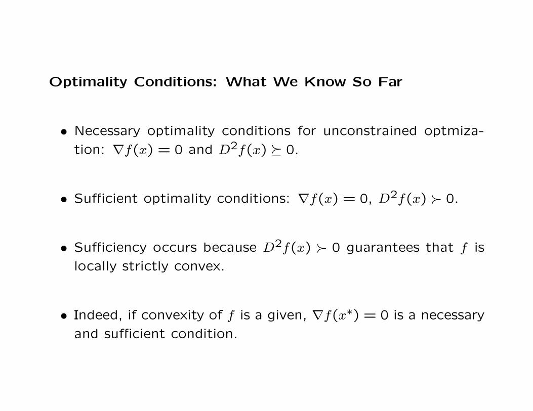
Optimality Conditions: What We Know So Far
• Necessary optimality conditions for unconstrained optmiza-
tion: ∇f(x) = 0 and D2f(x) � 0.
• Sufficient optimality conditions: ∇f(x) = 0, D2f(x) � 0.
• Sufficiency occurs because D2f(x) � 0 guarantees that f is
locally strictly convex.
• Indeed, if convexity of f is a given, ∇f(x∗) = 0 is a necessary
and sufficient condition.
• In the exercises, we used the fundamental theorem of linear
inequalities to derive the LP duality theorem. This yielded
the necessary and sufficient optimality conditions
ATy = c, y ≥ 0
Ax ≤ b
cTx − bTy = 0
for the LP problem
(P) maxx∈Rn
cTx
s.t. Ax ≤ b.
• Writing (P) in the form
min f(x)
s.t. gi(x) ≥ 0 (i = 1, . . . , m),
the optimality conditions can be rewritten as
∇f(x) −m∑
i=1
yi∇gi(x) = 0
gi(x) ≥ 0 (i = 1, . . . , m)
yT(Ax − b) = 0, that is,[ g1(x) ... gm(x) ]y = 0.
• We will see that the last condition could have been strength-
ened to yigi(x) = 0 for all i.
• LP is the simplest example of a constrained convex optimi-
sation problem: minimise a convex function over a convex
domain. Again convexity implies that first order conditions
are enough.
More generally, let
(NLP) minx∈Rn
f(x)
s.t. gi(x) = 0, (i ∈ E),
gj(x) ≥ 0 (j ∈ I).
The following will emerge under appropriate regularity assump-
tions:
i) Convex problems have first order necessary and sufficient
optimality conditions.
ii) In general problems, second order conditions introduce local
convexity.
I. First Order Necessary Optimality Conditions
Definition 1 Let x∗ ∈ Rn be feasible for the problem (NLP).
We say that the inequality constraint gj(x) ≥ 0 is active at x∗ if
g(x∗) = 0. We write A(x∗) := {j ∈ I : gj(x∗) = 0} for the set of
indices corresponding to active inequality constraints.
Of course, equality constraints are always active, but we will
account for their indices separately.
If J ⊂ E ∪ I is a subset of indices, we will write
• gJ for the vector-valued map that has gi (i ∈ J ) as compo-
nents in some specific order,
• g for gE∪I.
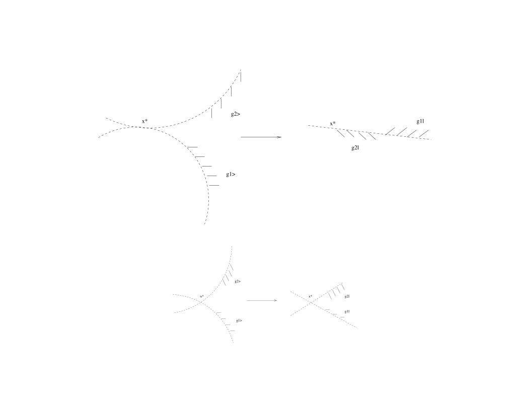
Definition 2: If {∇gi : i ∈ E ∪ A(x∗)} is a linearly independent
set of vectors, we say that the linear independence constraint
qualification (LICQ) holds at x∗.
g2l
x* g1lx*g2>
g1>
x* g2l
g1l
g2>
g1>
x*
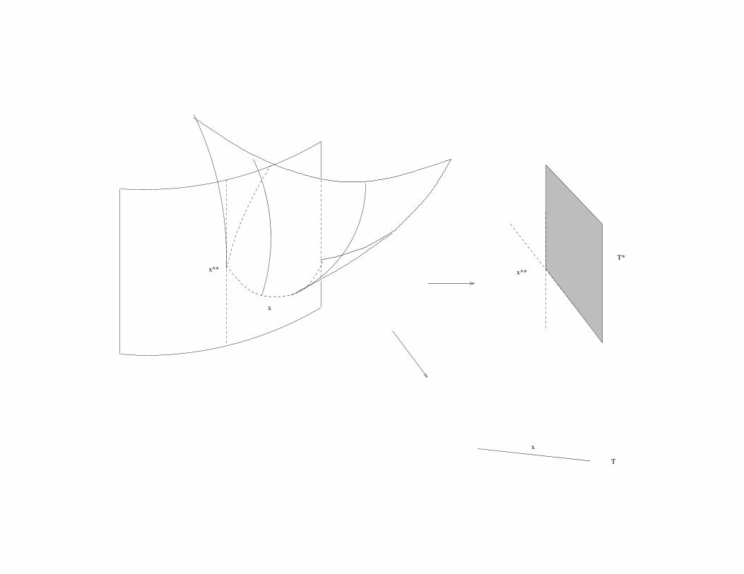
T
T*
x
x
x^*x^*
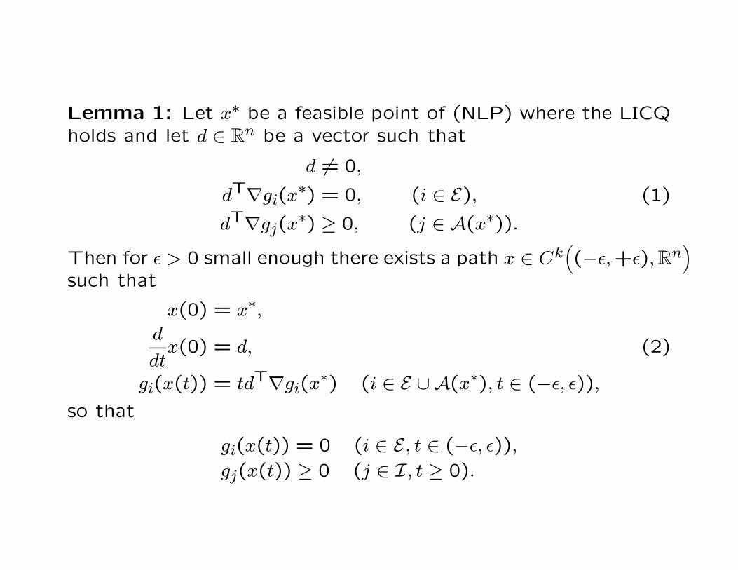
Lemma 1: Let x∗ be a feasible point of (NLP) where the LICQ
holds and let d ∈ Rn be a vector such that
d 6= 0,
dT∇gi(x∗) = 0, (i ∈ E),
dT∇gj(x∗) ≥ 0, (j ∈ A(x∗)).
(1)
Then for ε > 0 small enough there exists a path x ∈ Ck(
(−ε,+ε), Rn)
such that
x(0) = x∗,
d
dtx(0) = d,
gi(x(t)) = tdT∇gi(x∗) (i ∈ E ∪ A(x∗), t ∈ (−ε, ε)),
(2)
so that
gi(x(t)) = 0 (i ∈ E, t ∈ (−ε, ε)),
gj(x(t)) ≥ 0 (j ∈ I, t ≥ 0).
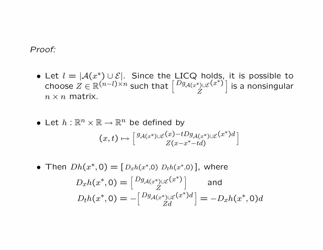
Proof:
• Let l = |A(x∗) ∪ E|. Since the LICQ holds, it is possible to
choose Z ∈ R(n−l)×n such that
[
DgA(x∗)∪E(x∗)
Z
]
is a nonsingular
n × n matrix.
• Let h : Rn × R → Rn be defined by
(x, t) 7→[ gA(x∗)∪E(x)−tDgA(x∗)∪E(x
∗)d
Z(x−x∗−td)
]
• Then Dh(x∗,0) = [ Dxh(x∗,0) Dth(x∗,0) ], where
Dxh(x∗,0) =[
DgA(x∗)∪E(x∗)
Z
]
and
Dth(x∗,0) = −[
DgA(x∗)∪E(x∗)d
Zd
]
= −Dxh(x∗,0)d
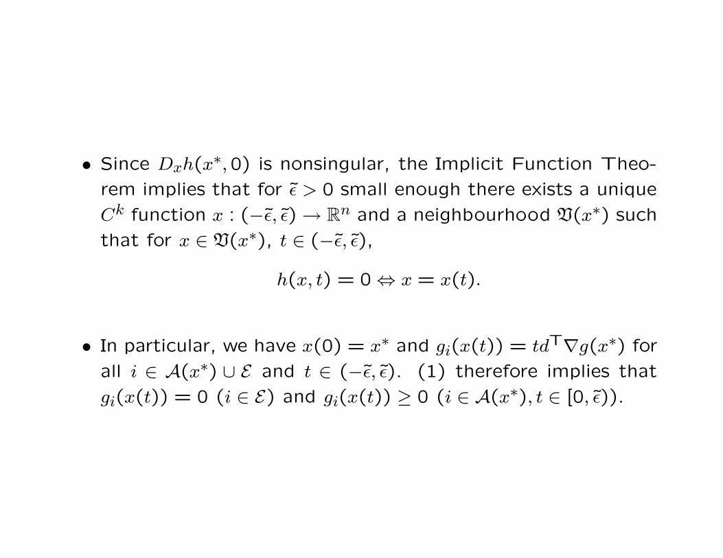
• Since Dxh(x∗,0) is nonsingular, the Implicit Function Theo-
rem implies that for ε̃ > 0 small enough there exists a unique
Ck function x : (−ε̃, ε̃) → Rn and a neighbourhood V(x∗) such
that for x ∈ V(x∗), t ∈ (−ε̃, ε̃),
h(x, t) = 0 ⇔ x = x(t).
• In particular, we have x(0) = x∗ and gi(x(t)) = tdT∇g(x∗) for
all i ∈ A(x∗) ∪ E and t ∈ (−ε̃, ε̃). (1) therefore implies that
gi(x(t)) = 0 (i ∈ E) and gi(x(t)) ≥ 0 (i ∈ A(x∗), t ∈ [0, ε̃)).
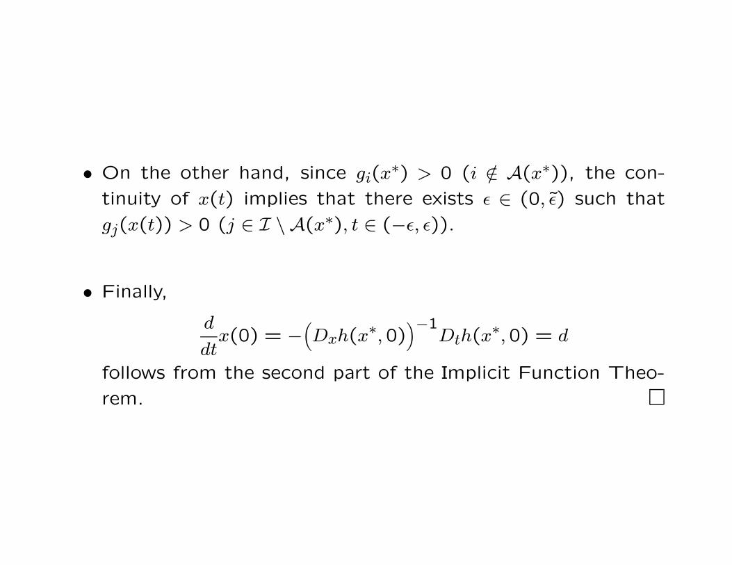
• On the other hand, since gi(x∗) > 0 (i /∈ A(x∗)), the con-
tinuity of x(t) implies that there exists ε ∈ (0, ε̃) such that
gj(x(t)) > 0 (j ∈ I \ A(x∗), t ∈ (−ε, ε)).
• Finally,
d
dtx(0) = −
(
Dxh(x∗,0))−1
Dth(x∗,0) = d
follows from the second part of the Implicit Function Theo-
rem.
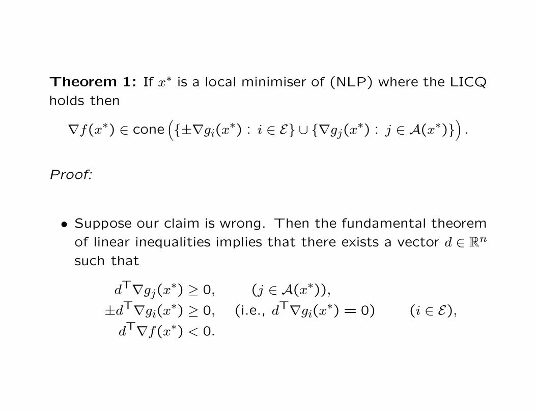
Theorem 1: If x∗ is a local minimiser of (NLP) where the LICQ
holds then
∇f(x∗) ∈ cone(
{±∇gi(x∗) : i ∈ E} ∪ {∇gj(x
∗) : j ∈ A(x∗)})
.
Proof:
• Suppose our claim is wrong. Then the fundamental theorem
of linear inequalities implies that there exists a vector d ∈ Rn
such that
dT∇gj(x∗) ≥ 0, (j ∈ A(x∗)),
±dT∇gi(x∗) ≥ 0, (i.e., dT∇gi(x
∗) = 0) (i ∈ E),
dT∇f(x∗) < 0.
• Since d satisfies (1), Lemma 1 implies that there exists a
path x : (−ε, ε) → Rn that satisfies (2).
• Taylor’s theorem then implies that
f(x(t)) = f(x∗) + td∇f(x∗) + O(t2) < f(x∗)
for 0 < t � 1.
• Since (2) shows that x(t) is feasible for t ∈ [0, ε), this con-
tradicts the assumption that x∗ is a local minimiser.
Comments:
• The condition
∇f(x∗) ∈ cone(
{±∇gi(x∗) : i ∈ E} ∪ {∇gj(x
∗) : j ∈ A(x∗)})
is equivalent to the existence of λ ∈ R|E∪I| such that
∇f(x∗) =∑
i∈E∪I
λi∇gi(x∗), (3)
where λj ≥ 0 (j ∈ A(x∗)) and λj = 0 for (j ∈ I \ A(x∗)).
• x∗ was assumed feasible, that is, gi(x∗) = 0 for all i ∈ E and
gj(x∗) ≥ 0 for all j ∈ I.
Thus, Theorem 1 shows that when x∗ is a local minimiser where
the LICQ holds, then the following so-called Karush-Kuhn-Tucker
(KKT) conditions must hold:
Corollary 1: There exist Lagrange multipliers λ ∈ R|I∪E| such
that
∇f(x) −∑
i∈I∪E
λi∇gi(x) = 0
gi(x) = 0 (i ∈ E)
gj(x) ≥ 0 (j ∈ I)
λjgj(x) = 0 (j ∈ I)
λj ≥ 0 (j ∈ I).
We can formulate this result in slightly more abstract form in
terms of the Lagrangian associated with (NLP):
L : Rn × R
m → R
(x, λ) 7→ f(x) −m∑
i=1
λigi(x).
The balance equation
∇f(x) −∑
i∈I∪E
λi∇gi(x) = 0
says that the derivative of the Lagrangian with respect to the x
coordinates is zero.
Putting all the pieces together, we obtain the following result:
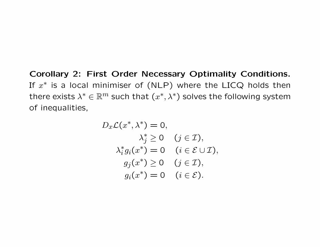
Corollary 2: First Order Necessary Optimality Conditions.
If x∗ is a local minimiser of (NLP) where the LICQ holds then
there exists λ∗ ∈ Rm such that (x∗, λ∗) solves the following system
of inequalities,
DxL(x∗, λ∗) = 0,
λ∗j ≥ 0 (j ∈ I),
λ∗i gi(x
∗) = 0 (i ∈ E ∪ I),
gj(x∗) ≥ 0 (j ∈ I),
gi(x∗) = 0 (i ∈ E).

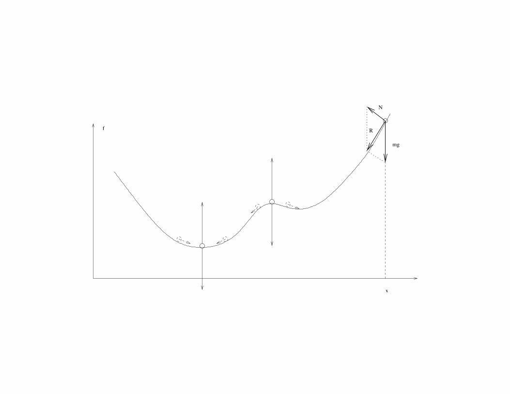
Mechanistic Motivation of KKT Conditions:
A useful picture in unconstrained optimisation is to imagine a
point mass m or an infinitesimally small ball that moves on a
hard surface
F :={
(x, f(x)) : x ∈ Rn}
without friction.
x
f
mg
N
R
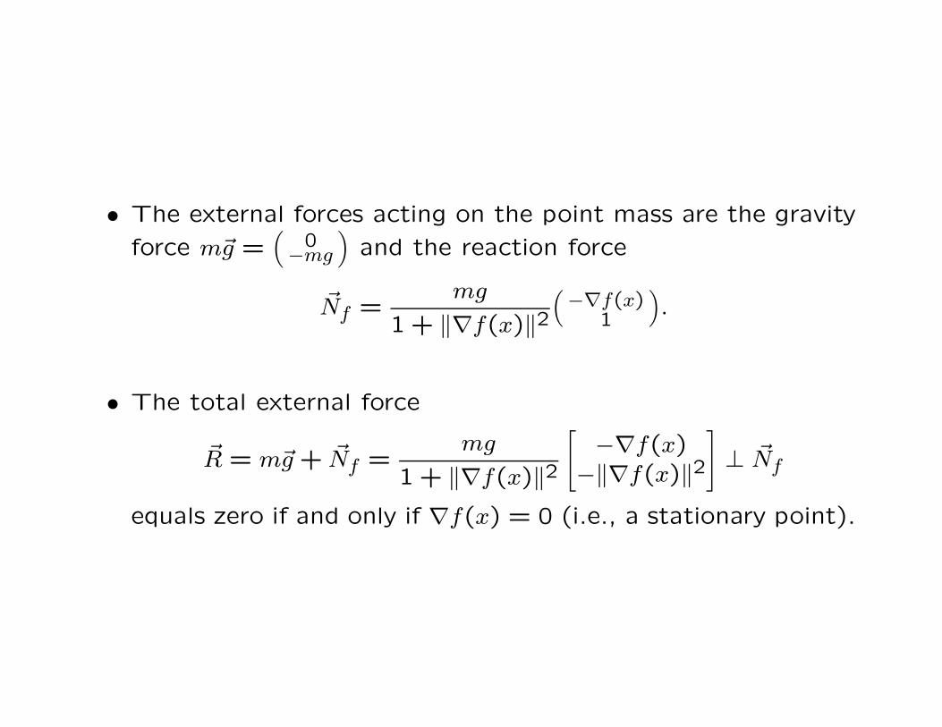
• The external forces acting on the point mass are the gravity
force m~g =(
0−mg
)
and the reaction force
~Nf =mg
1 + ‖∇f(x)‖2
(
−∇f(x)1
)
.
• The total external force
~R = m~g + ~Nf =mg
1 + ‖∇f(x)‖2
[
−∇f(x)
−‖∇f(x)‖2
]
⊥ ~Nf
equals zero if and only if ∇f(x) = 0 (i.e., a stationary point).
• When the test mass is slightly moved from a local maximiser,
then the external forces will pull it further away.
• In a neighbourhood of a local minimiser they will restore the
point mass to its former position.
• This is expressed by the second order optimality conditions:
an equilibrium position is stable if D2f(x) � 0 and instable if
D2f(x) ≺ 0.
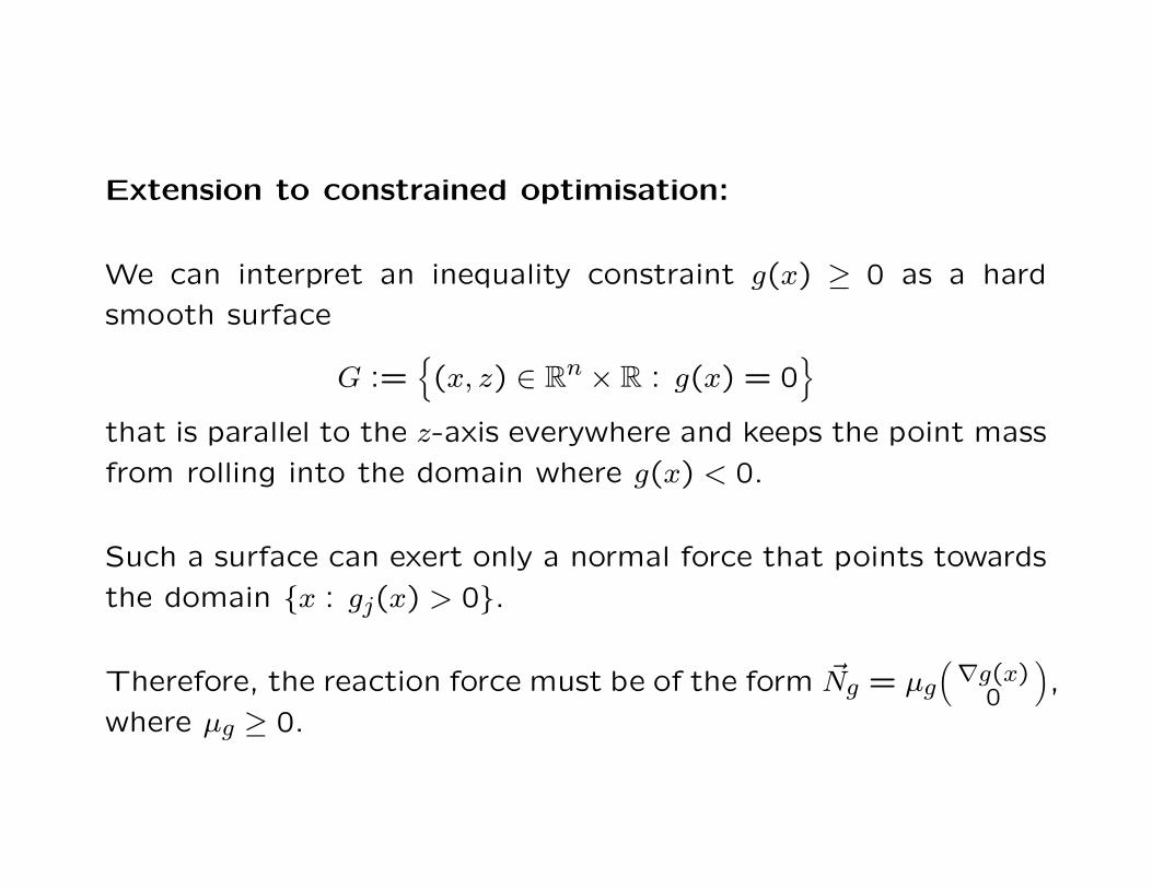
Extension to constrained optimisation:
We can interpret an inequality constraint g(x) ≥ 0 as a hard
smooth surface
G :={
(x, z) ∈ Rn × R : g(x) = 0
}
that is parallel to the z-axis everywhere and keeps the point mass
from rolling into the domain where g(x) < 0.
Such a surface can exert only a normal force that points towards
the domain {x : gj(x) > 0}.
Therefore, the reaction force must be of the form ~Ng = µg
(
∇g(x)0
)
,
where µg ≥ 0.
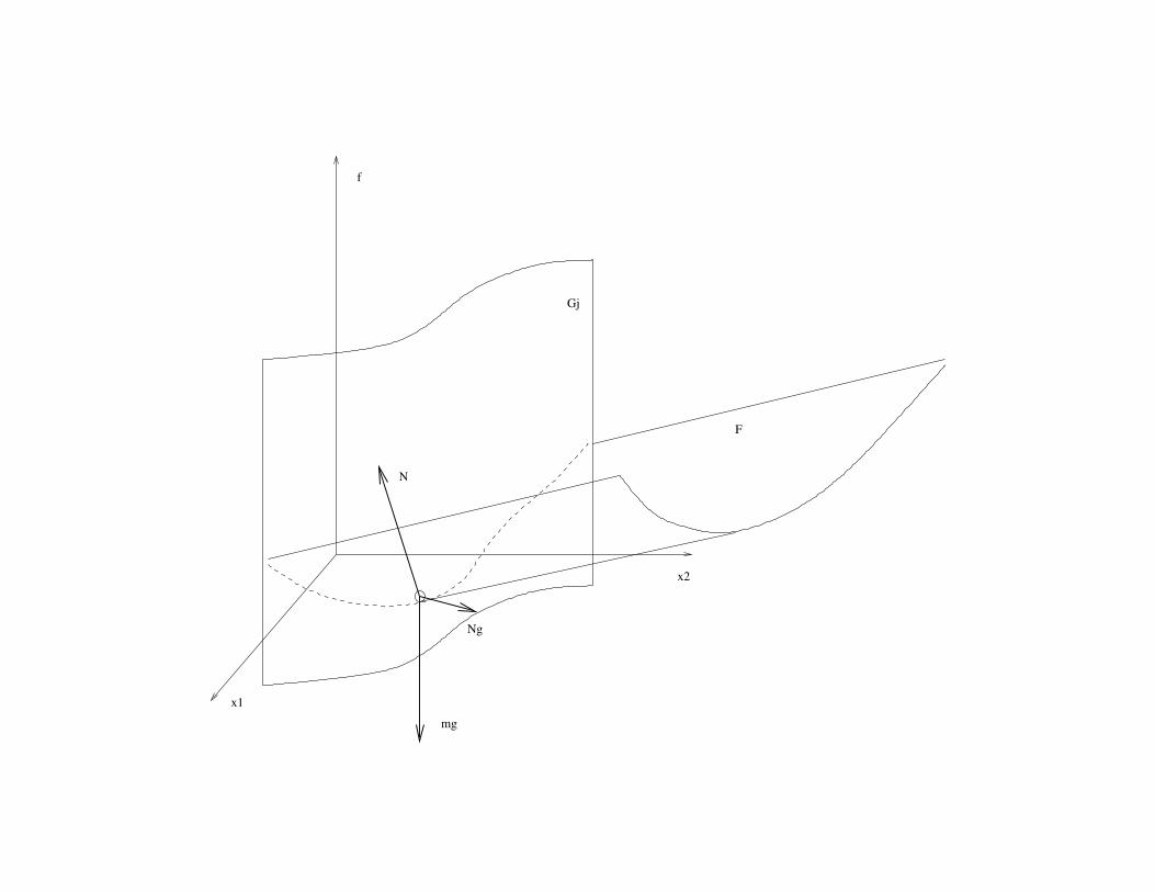
x2
x1
f
mg
N
Ng
F
Gj
• In the picture the point mass is at rest and does not roll to
lower terrain if the sum of external forces is zero, that is,~Nf + ~Ng + m~g = 0.
• Since ~Nf = µf
(
−∇f(x)1
)
for some µf ≥ 0, we find
µf
[
−∇f(x)1
]
+ µg
[
∇g(x)0
]
+
[
0−mg
]
= 0,
from where it follows that µf = mg and
∇f(x) = λ∇g(x) (4)
with λ = µ/mg ≥ 0.
• When multiple inequality constraints are present, the the bal-
ance equation (4) must thus be replaced with
∇f(x) =∑
j∈I
λj∇gj(x)
for some λj ≥ 0.
• Since constraints for which gj(x) > 0 cannot excert a force
on the test mass, we must set λj > 0 for these indices, or
equivalently, the equation λjgj(x) = 0 must hold for all j ∈ I.
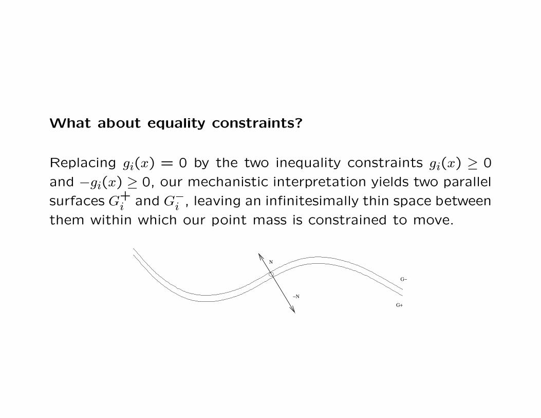
What about equality constraints?
Replacing gi(x) = 0 by the two inequality constraints gi(x) ≥ 0
and −gi(x) ≥ 0, our mechanistic interpretation yields two parallel
surfaces G+i and G−
i , leaving an infinitesimally thin space between
them within which our point mass is constrained to move.
−N
N
G−
G+
The net reaction force of the two surfaces is of the form
λ+i ∇gi(x) + λ−
i ∇(−gi)(x) = λi∇gi(x),
where we replaced the difference λ+i −λ−
i of the bound-constrained
variables λ+i , λ−
i ≥ 0 by a single unconstrained variable λi =
λ+i − λ−
i .
Note that in this case the conditions λ+i gi(x) = 0, λ−
i (−gi(x)) = 0
are satisfied automatically, since gi(x) = 0 if x is feasible.
G2
f
N2
N1
N
x*
x1
F
G1
x2

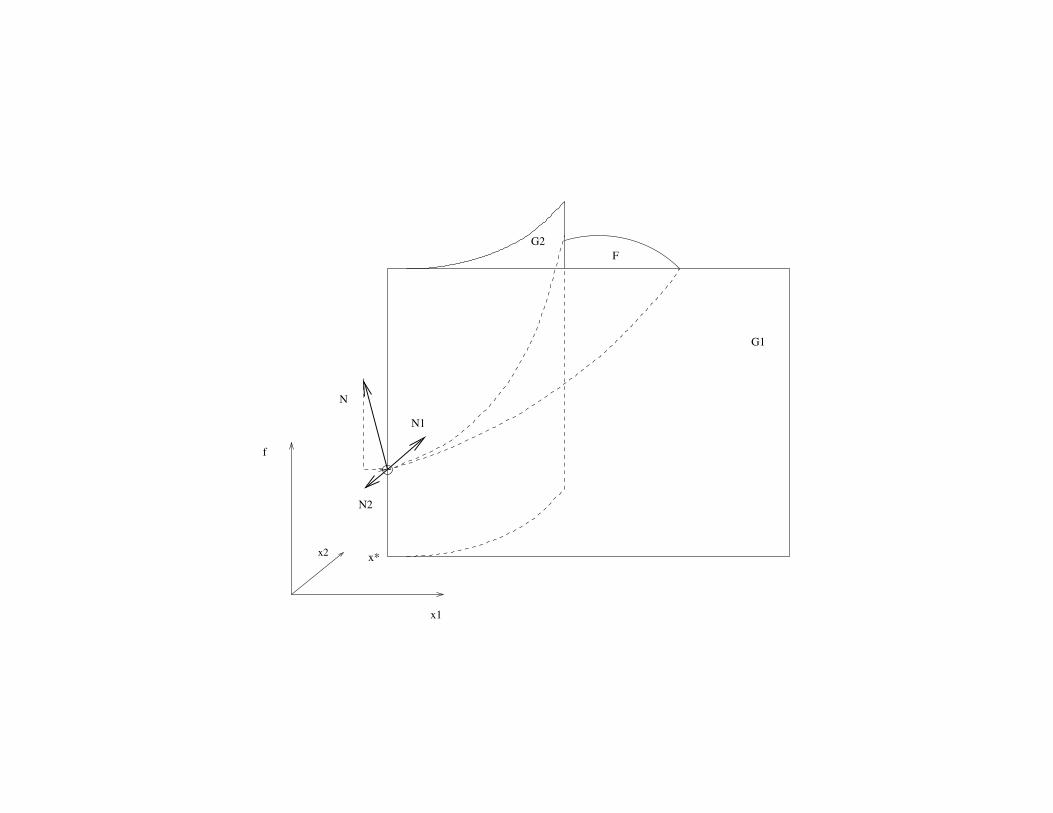
There are situations in which our mechanical picture is flawed:
if two inequality constraints have first order contact at a local
minimiser then they cannot annul the horizontal part of ~Nf .
When there are more constraints constraints, then generalisa-
tions of this situation can occur. In order to prove the KKT
conditions, we must therefore make a regularity assumption like
the LICQ.

Reading Assignment: Lecture-Note 9.