Embed Size (px)
Citation preview
OPTIMALITY CONDITIONS FOR DISJUNCTIVEPROGRAMS WITH APPLICATION TOMATHEMATICAL PROGRAMS WITH
EQUILIBRIUM CONSTRAINTS
Michael L. Flegel 1, Christian Kanzow 2, and Jirı V. Outrata 3
Preprint 256 October 2004
1,2 University of WurzburgInstitute of Applied Mathematics and StatisticsAm Hubland97074 WurzburgGermany
e-mail: [email protected]@mathematik.uni-wuerzburg.de
3 Academy of SciencesInstitute of Information Theory and Automation18208 PragueCzech Republic
e-mail: [email protected]
October 29, 2004
Abstract. We consider optimization problems with a disjunctive structure of the feasibleset. Using Guignard-type constraint qualifications for these optimization problems andexploiting some results for the limiting normal cone by Mordukhovich, we derive differentoptimality conditions. Furthermore, we specialize these results to mathematical programswith equilibrium constraints. In particular, we show that a new constraint qualification,weaker than any other constraint qualification used in the literature, is enough in orderto show that a local minimum results in a so-called M-stationary point. Additional as-sumptions are also discussed which guarantee that such an M-stationary point is in fact astrongly stationary point.
Key Words. disjunctive programs, mathematical programs with equilibrium constraints,M-stationarity, strong stationarity, Guignard constraint qualification.
1 Introduction
In the past decade applied mathematicians have been paying increasing interest to opti-mization problems where, among the constraints, so-called equilibrium constraints occur.This equilibrium is described mostly by a (lower-level) optimization problem, a variationalinequality or a complementarity problem. Following [10], all these problems are currentlytermed mathematical programs with equilibrium constraints, or MPECs. Most of them canbe written down in form of (smooth) nonlinear programs which, however, do not satisfymost of the standard constraint qualifications (CQs). This has lead to several weakenedstationarity notions that have been introduced in connection with optimality conditionsand numerical approaches.
Among these new stationarity notions an important role is played by a concept as-sociated with the generalized differential calculus of Mordukhovich, cf. [26, 13, 24, 14].Following [19], we will call it M-stationarity. The advantage of this concept consists, aboveall, in the fact that it requires only very weak constraint qualifications, cf. [4, 25]. Simul-taneously, starting with [10], another, stronger, stationarity notion has been investigated([23, 15]), referred to by the moniker strong stationarity in [19]. Strong stationarity is thenatural candidate for a stationarity concept for MPECs, because it is equivalent to thestandard KKT conditions if the MPEC can be expressed as a standard nonlinear program.As mentioned above, however, this stationarity concept is too restrictive in the context ofMPECs.
In this paper we will investigate the above mentioned stationarity notions by means of ageneral disjunctive program which embeds most MPECs considered in the literature so far.In particular, we will show that local minimizers are M-stationary under an appropriatevariant of the Guignard CQ [7], known to be the weakest CQ used in classical nonlinearprogramming. Moreover, we will derive a new condition which, together with this variantof Guignard CQ, ensures the strong stationarity of local minimizers.
Finally, these results will then be translated to the language of MPECs where theconstraints are described by a complementarity problem. In particular, we will show thatM- and strong stationarity indeed amount to the well-known conditions common in theliterature of these programs. Additionally, a new constraint qualification is introduced tosuch MPECs by transferring the variant of Guignard CQ for our disjunctive programs toan MPEC setting. This yields the weakest result known to date, M-stationarity as a firstorder condition under this very weak CQ.
The organization of the paper is as follows. Section 2 is devoted to some preliminaryresults including important definitions and some initial observations. The main resultsfor the disjunctive program are collected in Section 3. Finally, in Section 4, we apply theresults of Section 3 to a standard MPEC, where the equilibrium is modelled by a nonlinearcomplementarity problem. We then close with some final remarks in Section 5.
Our notation is standard. The n-dimensional Euclidean space is denoted by Rn, itsnonnegative and nonpositive orthant by Rn
+ and Rn−, respectively. If unclear from context,
the size of a zero vector is denoted by an appropriate subscript: 0n is the zero vector in Rn.Given a vector x ∈ Rn, its components are denoted by xi. Furthermore, given an index
3
set ω ⊆ 1, . . . , n, we denote by xω ∈ R|ω| the vector consisting of those componentsxi corresponding to the indices in ω. The same terminology applies to functions. Givena function F : Rn → Rm, we denote its Jacobian by ∇F (z) ∈ Rm×n. If m = 1, thegradient ∇F (z) ∈ Rn is considered a column vector. We call a set valued function amultifunction. Given such a multifunction Φ : Rp ⇒ Rq, its graph is defined by gph Φ :=(u, v) ∈ Rp+q | v ∈ Φ(u). Finally, given an arbitrary set K ⊆ Rn, it’s polar is defined byK := v ∈ Rn | vT w ≤ 0∀w ∈ K.
2 Preliminaries
For the reader’s convenience we start with the definitions of several basic notions in vari-ational analysis which will be extensively used throughout the paper.
Let A ⊆ Rn be an arbitrary closed set and u ∈ A. The nonempty cone
TA(u) := lim supτ0
A− u
τ
:= d ∈ Rn | ∃uk ⊂ A,∃τk 0 : uk → u,uk − u
τk
→ d
is called the contingent (also Bouligand or tangent) cone to A at u. Consider the familyof closed sets Ai, i = 1, . . . , k, and a point u ∈
⋂ki=1 Ai. Then it follows directly from the
above definition that
TSki=1 Ai
(u) =k⋃
i=1
TAi(u). (1)
Furthermore, we use the contingent cone to define the Frechet normal cone
NA(u) := (TA(u)) (2)
to A at u. Note that the Frechet normal cone is sometimes referred to as the regularnormal cone. This is most notably the case in [18]. Again, if we consider the family ofclosed sets Ai, i = 1, . . . , k, and a point x ∈
⋂ki=1 Ai, it follows from (1) and the properties
of the polar cone that
NSki=1 Ai
(u) =(TSk
i=1 Ai(u)
)=
k⋂i=1
(TAi(u)) =
k⋂i=1
NAi(u) (3)
(see [1, Theorem 3.1.9]).The cornerstone of the generalized differential calculus of Mordukhovich is the limiting
normal cone, also called the Mordukhovich normal cone, defined by
NA(u) := lim supu′
A→u
NA(u′)
:= limk→∞
wk | ∃uk ⊂ A : limk→∞
uk = u, wk ∈ NA(uk).
4
In contrast to the Frechet normal cone, NA(u) can be nonconvex, but admits a widelydeveloped calculus, cf. [11, 18]. In this calculus, an important role is played by stabilityof multifunctions reflecting the local structure of A. This will become important when weintroduce constraint qualifications further down. Note that if NA(u) = NA(u), we say thatthe set A is (normally) regular at u.
Consider now the general mathematical program
minimize f(z)subject to F (z) ∈ Λ,
(4)
where f : Rn → R, F : Rn → Rm are continuously differentiable functions and Λ ⊆ Rm isa nonempty closed (possibly nonconvex) set. It is clear that the constraint F (z) ∈ Λ canalso incorporate geometric constraints of the form z ∈ Ω, where Ω ⊆ Rn is an arbitraryclosed set.
Utilizing the normal cones introduced above, we are now able to define two stationarityconcepts which will play a central role in this paper.
Definition 2.1 Let z be feasible for the program (4).
(a) We say that z is M-stationary if there exists a KKT vector λ ∈ NΛ(F (z)) such that
0 = ∇f(z) + (∇F (z))T λ. (5)
(b) We say that z is strongly stationary if there exists a KKT vector λ ∈ NΛ(F (z)) suchthat
0 = ∇f(z) + (∇F (z))T λ. (6)
Note that M- and strong stationarity may be expressed as
0 ∈ ∇f(z) + (∇F (z))T NΛ(F (z))
and0 ∈ ∇f(z) + (∇F (z))T NΛ(F (z)),
respectively.The name M-stationarity is motivated by the fact that it involves the Mordukhovich
normal cone. It was coined in the context of MPECs by Scholtes [20]. Similarly, we usethe name strong stationarity in accordance with [19], where it was also used in the contextof MPECs. In the MPEC setting, strong stationarity is sometimes also referred to asprimal-dual stationarity [15].
As already mentioned, M-stationarity is a weaker stationarity concept than strongstationarity. However, the limiting normal cone (though nonconvex in general) has anextensive calculus, whereas the fuzzy calculus, developed for the Frechet normal cone isnot useful for our purposes.
Having introduced stationarity concepts for the program (4), we now turn our attentionto constraint qualifications. To this end, we need the concept of calmness of multifunctionsand the closely related idea of upper Lipschitz continuity.
5
Definition 2.2 Let Φ : Rp ⇒ Rq be a multifunction with a closed graph and (u, v) ∈ gph Φ.We say that Φ is calm at (u, v) provided there exist neighborhoods U of u, V of v, and amodulus L ≥ 0 such that
Φ(u′) ∩ V ⊂ Φ(u) + L‖u′ − u‖B for all u′ ∈ U . (7)
If (7) holds true with V = Rq, Φ is said to be locally upper Lipschitz continuous at u, cf.[17].
Note that calmness is sometimes also referred to as pseudo upper Lipschitz continuity(see, e.g., [26]) and that in [18] both calmness and local upper Lipschitz continuity arereferred to as calmness.
To obtain a constraint qualification for the program (4), we define a multifunctionM : Rm ⇒ Rn associated with the constraint system of (4) in the following fashion:
M(p) := z ∈ Rn |F (z) + p ∈ Λ . (8)
We can now use this multifunction to define a constraint qualification under which M-stationarity is a first order optimality condition. This is made precise in the followingtheorem, a proof of which may be found, e.g., in [14, Theorem 2.4].
Theorem 2.3 Let z be a local minimizer of (4). If the multifunction M (see (8)) is calmat (0, z), z is M-stationary.
Note that if we drop the continuous differentiability of f and F in favor of Lipschitzcontinuity near z of these functions, the result of Theorem 2.3 remains true if we stateM-stationarity (5) in terms of the subgradient of f and the coderivative of an appropriatefunction, see [26] for details.
A constraint qualification better known in nonlinear programming is the Mangasarian-Fromovitz constraint qualification (MFCQ). We define a generalization of this CQ.
Definition 2.4 Let z be feasible for the program (4). We say that the generalized Manga-sarian-Fromovitz constraint qualification (GMFCQ) holds at z if the implication
∇F (z)T λ = 0
λ ∈ NΛ(F (z))
=⇒ λ = 0 (9)
holds.
If Λ = Rm− , the condition (9) reduces to the classical Mangasarian-Fromovitz constraint
qualification, justifying the name GMFCQ.We now show that M-stationarity is a first order condition under GMFCQ.
Corollary 2.5 Let z be a local minimizer of the program (4) at which GMFCQ holds.Then z is M-stationary.
6
Proof. Due to Theorem 2.3, it suffices to show that GMFCQ implies the calmness of M at(0, z). From [12, Corollary 4.4], we readily infer that GMFCQ implies the so-called Aubinproperty of M around (0, z). Since this property is stronger than the required calmness(see, e.g., [18, Definition 9.36]), the result follows.
For more information on the Aubin property, we refer the reader to the book by Rock-afellar and Wets [18].
Having discussed both calmness and GMFCQ as constraint qualifications, we now in-troduce generalizations of the Abadie and Guignard constraint qualifications known fromstandard nonlinear programming.
Definition 2.6 Let z be feasible for the program (4).
(a) We say that the generalized Abadie constraint qualification (GACQ) holds at z if
TF−1(Λ)(z) = L(z), (10)
whereL(z) := h ∈ Rn | ∇F (z) h ∈ TΛ(F (z)) (11)
is called the linearized cone at z.
(b) We say that the generalized (or dual) Guignard constraint qualification (GGCQ)holds at z if
NF−1(Λ)(z) = (L(z)) . (12)
To justify the names of the above constraint qualifications, we apply them to a standardnonlinear program that takes the form
minimize f(z)subject to g(z) ≤ 0, h(z) = 0,
(13)
with continuously differentiable f : Rn → R, g : Rn → Rm, and h : Rn → Rp. To formulatethis program in the fashion of (4), we set
F (z) := (g(z), h(z)) and Λ := Rm− × 0p.
It is then easily verified that
L(z) = d ∈ Rn | ∇gi(z)T d ≤ 0, ∀i ∈ Ig,
∇hi(z)T d = 0, ∀i = 1, . . . , p ,
where Ig := i | gi(z) = 0 is the set of active inequality constraints.Clearly, in this case GACQ and GGCQ reduce to the standard definitions of Abadie
and Guignard CQ, respectively, as they are most commonly stated, see, e.g., [1]. However,Guignard [7] originally stated her CQ in the primal form. Her definition is equivalent to
7
the above dual characterization of Guignard CQ if Λ is convex. In the nonconvex casethe relationship is not as straightforward. Since Guignard CQ is commonly defined usingthe dual formulation (see, e.g., [16, 1, 6, 21]), however, we feel justified in calling (12) thegeneralized Guignard CQ.
Note that since NF−1(Λ)(z) = TF−1(Λ)(z) by definition (see (2)), GACQ at z obviouslyimplies GGCQ at z. Furthermore, as proved in [9, Proposition 1], calmness of M at (0, z)implies GACQ at z. Together with the discussion preceding Corollary 2.5, this yields thefollowing chain of implications:
GMFCQ at z =⇒ calmness of M at (0, z) =⇒ GACQ at z =⇒ GGCQ at z. (14)
In general, none of the implications can be reversed. Specifically, the following exampledemonstrates that GGCQ does not, in general, imply GACQ.
Example 2.7 Consider the program
minimize z21 + z2
2
subject to
[z21
z22
]∈ Λ := Λ1 ∪ Λ2,
with Λ1 := R+ × 0 and Λ2 := 0 × R+. Obviously, the origin is the unique minimizer.It is then easily verified that the contingent cone takes the form
TF−1(Λ)(0) = h ∈ R2 | h1h2 = 0,
while the linearized cone takes the form
L(0) = h ∈ R2 | (0, 0)h ∈ TΛ(0) = R2.
Obviously, TF−1(Λ)(0) 6= L(0), so GACQ is not satisfied. However, it is easily verified that
TF−1(Λ)(0) = 0 = L(0),
demonstrating that GGCQ does hold.
An important question surrounding GACQ and GGCQ is their connection with op-timality conditions. It is known that if Λ is convex, strong stationarity is a first orderoptimality condition under GGCQ and hence under GACQ (see the arguments followingDefinition 2.6). In the following sections we will investigate how this can be extended tononconvex Λ.
Another question is when we might expect strong stationarity to be a first order opti-mality condition. Since f is continuously differentiable, we have the well-known optimalitycondition
0 ∈ ∇f(z) + NF−1(Λ)(z), (15)
cf., e.g., [18, Theorem 6.12]. Unfortunately, we only have the inclusion
NF−1(Λ)(z) ⊃ (∇F (z))T NΛ (F (z)) (16)
8
which turns out to be an equality provided GMFCQ is satisfied at z and Λ is (normally)regular at F (z) (see [18, Theorem 6.14]). However, this condition never holds for equilib-rium constraints. This question is important, because we need to have equality in (16) inorder to explicitly determine the cone NF−1(Λ)(z), and with it to be able to verify whetherstrong stationarity holds.
3 The Disjunctive Program
In this section we will investigate GACQ and GGCQ in context with M- and strong sta-tionarity under the structural assumption that
Λ =k⋃
i=1
Λi, (17)
where all Λi, i = 1, . . . , k, are convex polyhedra. This assumption is satisfied by a largeclass of equilibrium constraints, see Section 4 for an example of this.
The sets Λi are called components and with each z ∈ Λ we associate the index set I(z)of active components defined by
I(z) := i ∈ 1, . . . , k | F (z) ∈ Λi .
For the remainder of this section, we will confine ourselves to the program
minimize f(z)
subject to F (z) ∈ Λ =⋃k
i=1 Λi,(18)
where the constraints are given by (17).For such a program, we are indeed able to show that M-stationarity is a necessary first
order condition under GGCQ and hence GACQ.
Theorem 3.1 Let z be a local minimizer of the program (18). Then, if GGCQ is satisfiedat z, z is M-stationary.
Proof. As mentioned in the previous section, relation (15) holds true. Thus, due to GGCQat z, one has
0 ∈ ∇f(z) + (L(z)). (19)
By definition of the polar cone, this means that h = 0 is the (unique) solution of theprogram
minimize ∇f(z)T hsubject to ∇F (z) h ∈ TΛ(F (z)).
(20)
By virtue of (1),
TΛ(F (z)) =⋃
i∈I(z)
TΛi(F (z)).
9
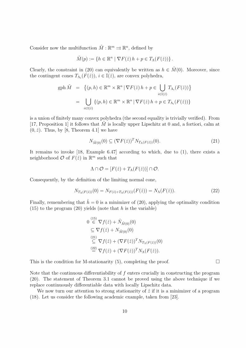
Consider now the multifunction M : Rm ⇒ Rn, defined by
M(p) := h ∈ Rn | ∇F (z) h + p ∈ TΛ(F (z)) .
Clearly, the constraint in (20) can equivalently be written as h ∈ M(0). Moreover, sincethe contingent cones TΛi
(F (z)), i ∈ I(z), are convex polyhedra,
gph M =(p, h) ∈ Rm × Rn |∇F (z) h + p ∈
⋃i∈I(z)
TΛi(F (z))
=
⋃i∈I(z)
(p, h) ∈ Rm × Rn |∇F (z) h + p ∈ TΛi(F (z))
is a union of finitely many convex polyhedra (the second equality is trivially verified). From[17, Proposition 1] it follows that M is locally upper Lipschitz at 0 and, a fortiori, calm at(0, z). Thus, by [8, Theorem 4.1] we have
NM(0)(0) ⊆ (∇F (z))T NTΛ(F (z))(0). (21)
It remains to invoke [18, Example 6.47] according to which, due to (1), there exists aneighborhood O of F (z) in Rm such that
Λ ∩ O = [F (z) + TΛ(F (z))] ∩ O.
Consequently, by the definition of the limiting normal cone,
NTΛ(F (z))(0) = NF (z)+TΛ(F (z))(F (z)) = NΛ(F (z)). (22)
Finally, remembering that h = 0 is a minimizer of (20), applying the optimality condition(15) to the program (20) yields (note that h is the variable)
0(15)∈ ∇f(z) + NM(0)(0)
⊆ ∇f(z) + NM(0)(0)
(21)
⊆ ∇f(z) + (∇F (z))T NTΛ(F (z))(0)
(22)= ∇f(z) + (∇F (z))T NΛ(F (z)).
This is the condition for M-stationarity (5), completing the proof.
Note that the continuous differentiability of f enters crucially in constructing the program(20). The statement of Theorem 3.1 cannot be proved using the above technique if wereplace continuously differentiable data with locally Lipschitz data.
We now turn our attention to strong stationarity of z if it is a minimizer of a program(18). Let us consider the following academic example, taken from [23].
10
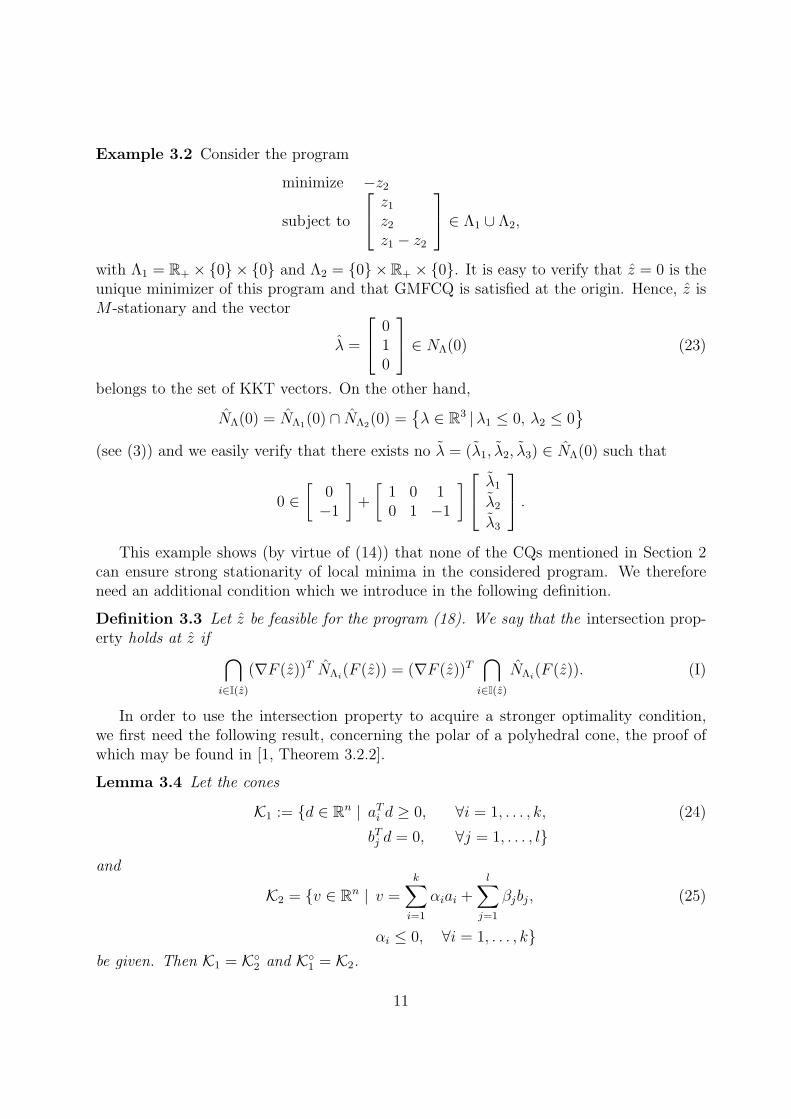
Example 3.2 Consider the program
minimize −z2
subject to
z1
z2
z1 − z2
∈ Λ1 ∪ Λ2,
with Λ1 = R+ × 0 × 0 and Λ2 = 0 ×R+ × 0. It is easy to verify that z = 0 is theunique minimizer of this program and that GMFCQ is satisfied at the origin. Hence, z isM -stationary and the vector
λ =
010
∈ NΛ(0) (23)
belongs to the set of KKT vectors. On the other hand,
NΛ(0) = NΛ1(0) ∩ NΛ2(0) =λ ∈ R3 |λ1 ≤ 0, λ2 ≤ 0
(see (3)) and we easily verify that there exists no λ = (λ1, λ2, λ3) ∈ NΛ(0) such that
0 ∈[
0−1
]+
[1 0 10 1 −1
] λ1
λ2
λ3
.
This example shows (by virtue of (14)) that none of the CQs mentioned in Section 2can ensure strong stationarity of local minima in the considered program. We thereforeneed an additional condition which we introduce in the following definition.
Definition 3.3 Let z be feasible for the program (18). We say that the intersection prop-erty holds at z if ⋂
i∈I(z)
(∇F (z))T NΛi(F (z)) = (∇F (z))T
⋂i∈I(z)
NΛi(F (z)). (I)
In order to use the intersection property to acquire a stronger optimality condition,we first need the following result, concerning the polar of a polyhedral cone, the proof ofwhich may be found in [1, Theorem 3.2.2].
Lemma 3.4 Let the cones
K1 := d ∈ Rn | aTi d ≥ 0, ∀i = 1, . . . , k,
bTj d = 0, ∀j = 1, . . . , l
(24)
and
K2 = v ∈ Rn | v =k∑
i=1
αiai +l∑
j=1
βjbj,
αi ≤ 0, ∀i = 1, . . . , k
(25)
be given. Then K1 = K2 and K
1 = K2.
11
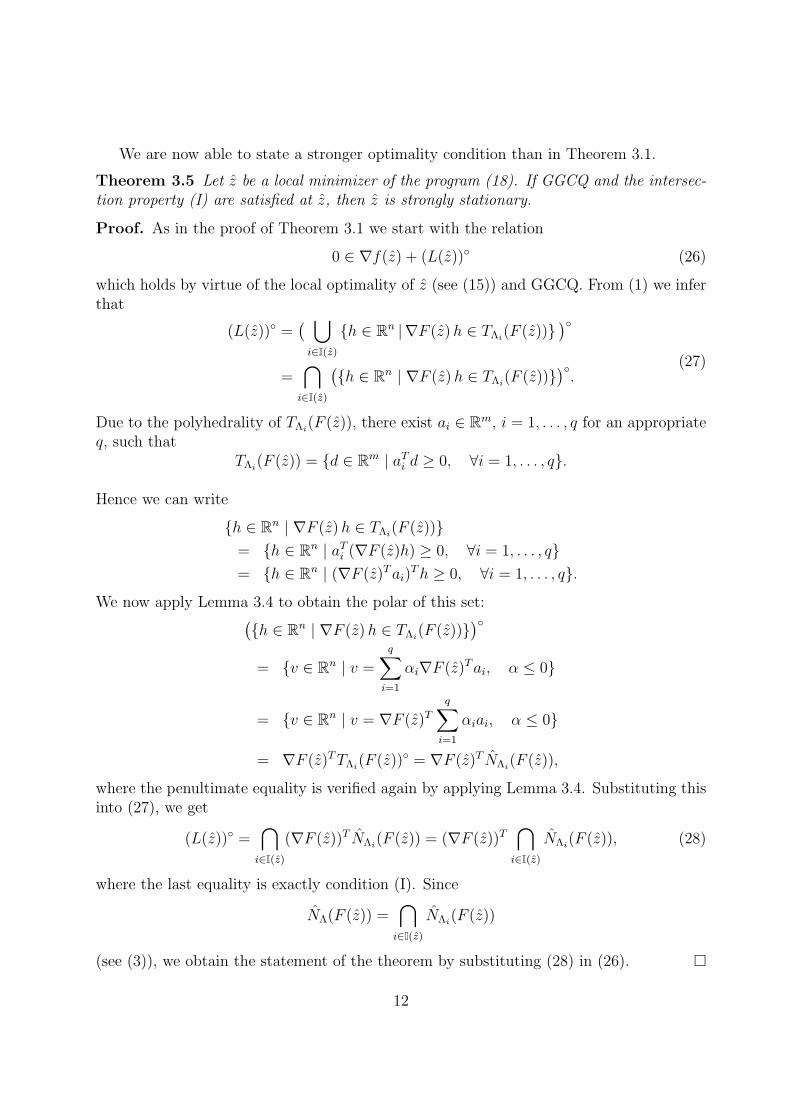
We are now able to state a stronger optimality condition than in Theorem 3.1.
Theorem 3.5 Let z be a local minimizer of the program (18). If GGCQ and the intersec-tion property (I) are satisfied at z, then z is strongly stationary.
Proof. As in the proof of Theorem 3.1 we start with the relation
0 ∈ ∇f(z) + (L(z)) (26)
which holds by virtue of the local optimality of z (see (15)) and GGCQ. From (1) we inferthat
(L(z)) =( ⋃
i∈I(z)
h ∈ Rn |∇F (z) h ∈ TΛi(F (z))
)=
⋂i∈I(z)
(h ∈ Rn | ∇F (z) h ∈ TΛi
(F (z)))
.(27)
Due to the polyhedrality of TΛi(F (z)), there exist ai ∈ Rm, i = 1, . . . , q for an appropriate
q, such thatTΛi
(F (z)) = d ∈ Rm | aTi d ≥ 0, ∀i = 1, . . . , q.
Hence we can write
h ∈ Rn | ∇F (z) h ∈ TΛi(F (z))
= h ∈ Rn | aTi (∇F (z)h) ≥ 0, ∀i = 1, . . . , q
= h ∈ Rn | (∇F (z)T ai)T h ≥ 0, ∀i = 1, . . . , q.
We now apply Lemma 3.4 to obtain the polar of this set:(h ∈ Rn | ∇F (z) h ∈ TΛi
(F (z)))
= v ∈ Rn | v =
q∑i=1
αi∇F (z)T ai, α ≤ 0
= v ∈ Rn | v = ∇F (z)T
q∑i=1
αiai, α ≤ 0
= ∇F (z)T TΛi(F (z)) = ∇F (z)T NΛi
(F (z)),
where the penultimate equality is verified again by applying Lemma 3.4. Substituting thisinto (27), we get
(L(z)) =⋂
i∈I(z)
(∇F (z))T NΛi(F (z)) = (∇F (z))T
⋂i∈I(z)
NΛi(F (z)), (28)
where the last equality is exactly condition (I). Since
NΛ(F (z)) =⋂
i∈I(z)
NΛi(F (z))
(see (3)), we obtain the statement of the theorem by substituting (28) in (26).
12
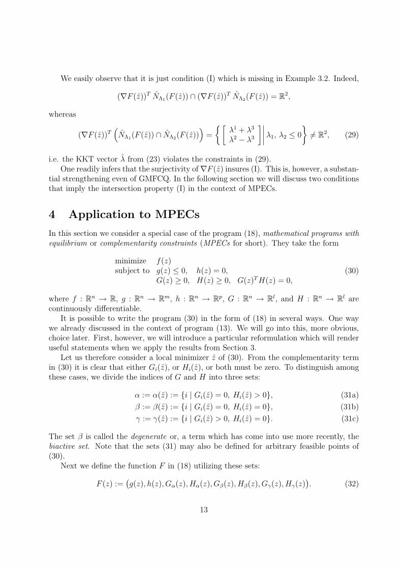
We easily observe that it is just condition (I) which is missing in Example 3.2. Indeed,
(∇F (z))T NΛ1(F (z)) ∩ (∇F (z))T NΛ2(F (z)) = R2,
whereas
(∇F (z))T(NΛ1(F (z)) ∩ NΛ2(F (z))
)=
[λ1 + λ3
λ2 − λ3
]∣∣∣∣ λ1, λ2 ≤ 0
6= R2, (29)
i.e. the KKT vector λ from (23) violates the constraints in (29).One readily infers that the surjectivity of∇F (z) insures (I). This is, however, a substan-
tial strengthening even of GMFCQ. In the following section we will discuss two conditionsthat imply the intersection property (I) in the context of MPECs.
4 Application to MPECs
In this section we consider a special case of the program (18), mathematical programs withequilibrium or complementarity constraints (MPECs for short). They take the form
minimize f(z)subject to g(z) ≤ 0, h(z) = 0,
G(z) ≥ 0, H(z) ≥ 0, G(z)T H(z) = 0,(30)
where f : Rn → R, g : Rn → Rm, h : Rn → Rp, G : Rn → Rl, and H : Rn → Rl arecontinuously differentiable.
It is possible to write the program (30) in the form of (18) in several ways. One waywe already discussed in the context of program (13). We will go into this, more obvious,choice later. First, however, we will introduce a particular reformulation which will renderuseful statements when we apply the results from Section 3.
Let us therefore consider a local minimizer z of (30). From the complementarity termin (30) it is clear that either Gi(z), or Hi(z), or both must be zero. To distinguish amongthese cases, we divide the indices of G and H into three sets:
α := α(z) := i | Gi(z) = 0, Hi(z) > 0, (31a)
β := β(z) := i | Gi(z) = 0, Hi(z) = 0, (31b)
γ := γ(z) := i | Gi(z) > 0, Hi(z) = 0. (31c)
The set β is called the degenerate or, a term which has come into use more recently, thebiactive set. Note that the sets (31) may also be defined for arbitrary feasible points of(30).
Next we define the function F in (18) utilizing these sets:
F (z) :=(g(z), h(z), Gα(z), Hα(z), Gβ(z), Hβ(z), Gγ(z), Hγ(z)
). (32)
13
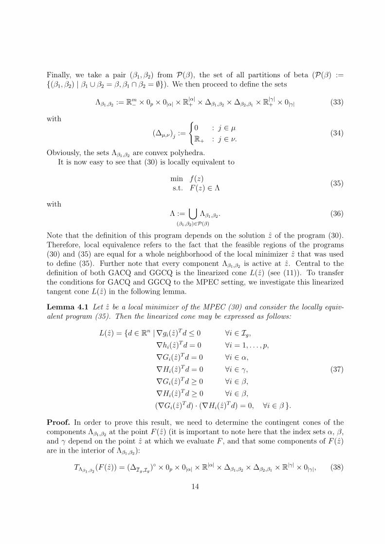
Finally, we take a pair (β1, β2) from P(β), the set of all partitions of beta (P(β) :=(β1, β2) | β1 ∪ β2 = β, β1 ∩ β2 = ∅). We then proceed to define the sets
Λβ1,β2 := Rm− × 0p × 0|α| × R|α|
+ ×∆β1,β2 ×∆β2,β1 × R|γ|+ × 0|γ| (33)
with
(∆µ,ν)j :=
0 : j ∈ µ
R+ : j ∈ ν.(34)
Obviously, the sets Λβ1,β2 are convex polyhedra.It is now easy to see that (30) is locally equivalent to
min f(z)s.t. F (z) ∈ Λ
(35)
withΛ :=
⋃Λβ1,β2 .
(β1,β2)∈P(β)
(36)
Note that the definition of this program depends on the solution z of the program (30).Therefore, local equivalence refers to the fact that the feasible regions of the programs(30) and (35) are equal for a whole neighborhood of the local minimizer z that was usedto define (35). Further note that every component Λβ1,β2 is active at z. Central to thedefinition of both GACQ and GGCQ is the linearized cone L(z) (see (11)). To transferthe conditions for GACQ and GGCQ to the MPEC setting, we investigate this linearizedtangent cone L(z) in the following lemma.
Lemma 4.1 Let z be a local minimizer of the MPEC (30) and consider the locally equiv-alent program (35). Then the linearized cone may be expressed as follows:
L(z) = d ∈ Rn |∇gi(z)T d ≤ 0 ∀i ∈ Ig,
∇hi(z)T d = 0 ∀i = 1, . . . , p,
∇Gi(z)T d = 0 ∀i ∈ α,
∇Hi(z)T d = 0 ∀i ∈ γ,
∇Gi(z)T d ≥ 0 ∀i ∈ β,
∇Hi(z)T d ≥ 0 ∀i ∈ β,
(∇Gi(z)T d) · (∇Hi(z)T d) = 0, ∀i ∈ β .
(37)
Proof. In order to prove this result, we need to determine the contingent cones of thecomponents Λβ1,β2 at the point F (z) (it is important to note here that the index sets α, β,and γ depend on the point z at which we evaluate F , and that some components of F (z)are in the interior of Λβ1,β2):
TΛβ1,β2(F (z)) = (∆Ig ,Ig
) × 0p × 0|α| × R|α| ×∆β1,β2 ×∆β2,β1 × R|γ| × 0|γ|, (38)
14
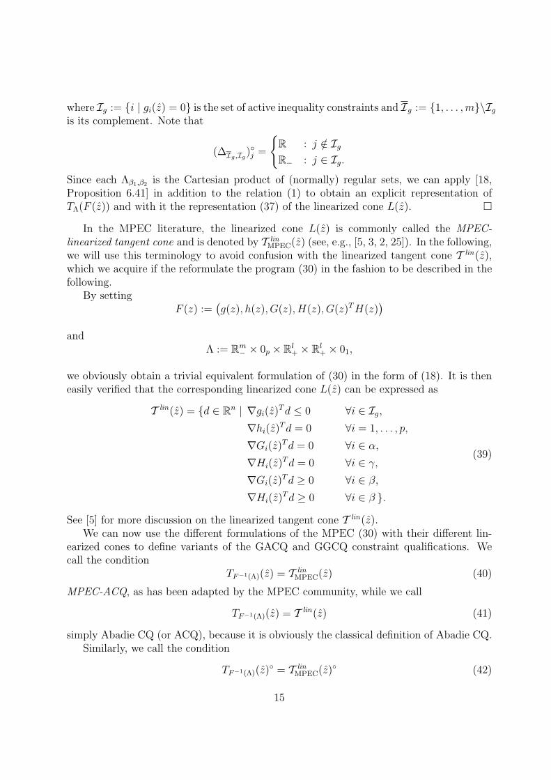
where Ig := i | gi(z) = 0 is the set of active inequality constraints and Ig := 1, . . . ,m\Ig
is its complement. Note that
(∆Ig ,Ig)j =
R : j /∈ Ig
R− : j ∈ Ig.
Since each Λβ1,β2 is the Cartesian product of (normally) regular sets, we can apply [18,Proposition 6.41] in addition to the relation (1) to obtain an explicit representation ofTΛ(F (z)) and with it the representation (37) of the linearized cone L(z).
In the MPEC literature, the linearized cone L(z) is commonly called the MPEC-linearized tangent cone and is denoted by T lin
MPEC(z) (see, e.g., [5, 3, 2, 25]). In the following,we will use this terminology to avoid confusion with the linearized tangent cone T lin(z),which we acquire if the reformulate the program (30) in the fashion to be described in thefollowing.
By settingF (z) :=
(g(z), h(z), G(z), H(z), G(z)T H(z)
)and
Λ := Rm− × 0p × Rl
+ × Rl+ × 01,
we obviously obtain a trivial equivalent formulation of (30) in the form of (18). It is theneasily verified that the corresponding linearized cone L(z) can be expressed as
T lin(z) = d ∈ Rn | ∇gi(z)T d ≤ 0 ∀i ∈ Ig,
∇hi(z)T d = 0 ∀i = 1, . . . , p,
∇Gi(z)T d = 0 ∀i ∈ α,
∇Hi(z)T d = 0 ∀i ∈ γ,
∇Gi(z)T d ≥ 0 ∀i ∈ β,
∇Hi(z)T d ≥ 0 ∀i ∈ β .
(39)
See [5] for more discussion on the linearized tangent cone T lin(z).We can now use the different formulations of the MPEC (30) with their different lin-
earized cones to define variants of the GACQ and GGCQ constraint qualifications. Wecall the condition
TF−1(Λ)(z) = T linMPEC(z) (40)
MPEC-ACQ, as has been adapted by the MPEC community, while we call
TF−1(Λ)(z) = T lin(z) (41)
simply Abadie CQ (or ACQ), because it is obviously the classical definition of Abadie CQ.Similarly, we call the condition
TF−1(Λ)(z) = T linMPEC(z) (42)
15
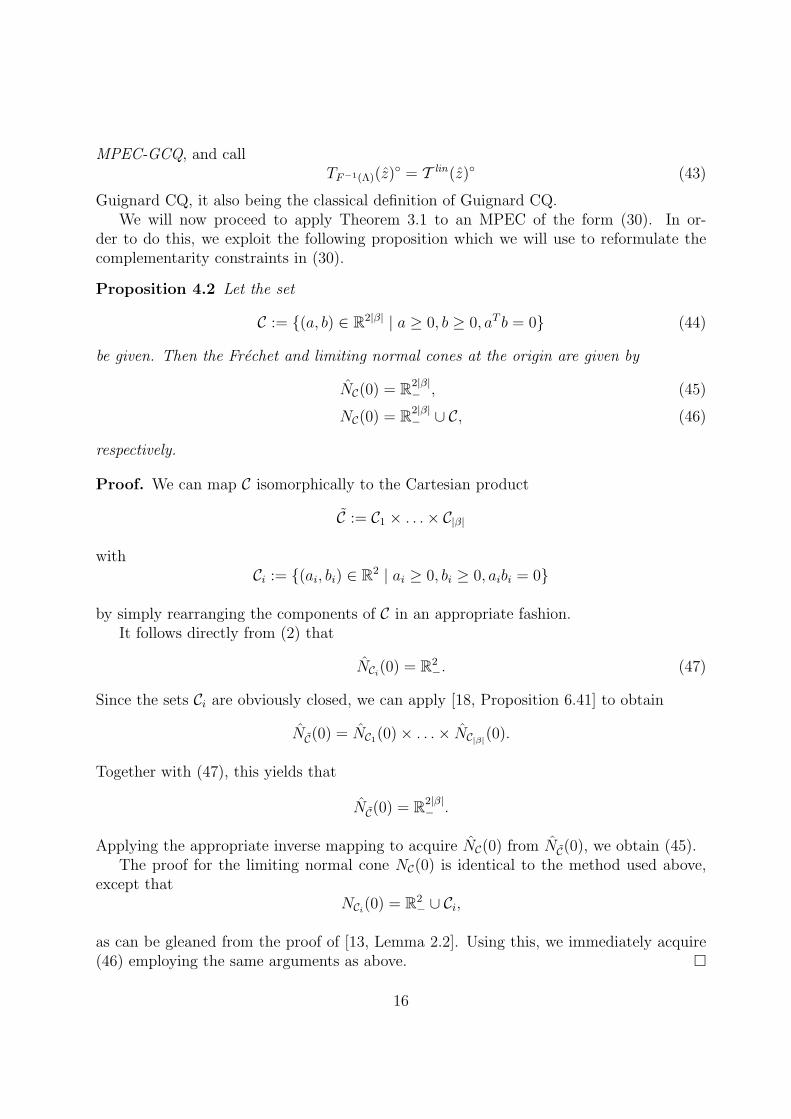
MPEC-GCQ, and callTF−1(Λ)(z) = T lin(z) (43)
Guignard CQ, it also being the classical definition of Guignard CQ.We will now proceed to apply Theorem 3.1 to an MPEC of the form (30). In or-
der to do this, we exploit the following proposition which we will use to reformulate thecomplementarity constraints in (30).
Proposition 4.2 Let the set
C := (a, b) ∈ R2|β| | a ≥ 0, b ≥ 0, aT b = 0 (44)
be given. Then the Frechet and limiting normal cones at the origin are given by
NC(0) = R2|β|− , (45)
NC(0) = R2|β|− ∪ C, (46)
respectively.
Proof. We can map C isomorphically to the Cartesian product
C := C1 × . . .× C|β|
withCi := (ai, bi) ∈ R2 | ai ≥ 0, bi ≥ 0, aibi = 0
by simply rearranging the components of C in an appropriate fashion.It follows directly from (2) that
NCi(0) = R2
−. (47)
Since the sets Ci are obviously closed, we can apply [18, Proposition 6.41] to obtain
NC(0) = NC1(0)× . . .× NC|β|(0).
Together with (47), this yields that
NC(0) = R2|β|− .
Applying the appropriate inverse mapping to acquire NC(0) from NC(0), we obtain (45).The proof for the limiting normal cone NC(0) is identical to the method used above,
except thatNCi
(0) = R2− ∪ Ci,
as can be gleaned from the proof of [13, Lemma 2.2]. Using this, we immediately acquire(46) employing the same arguments as above.
16
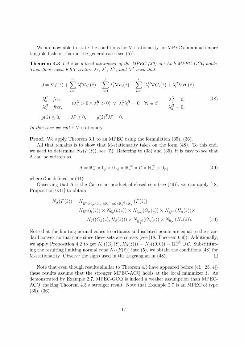
We are now able to state the conditions for M-stationarity for MPECs in a much moretangible fashion than in the general case (see (5)).
Theorem 4.3 Let z be a local minimizer of the MPEC (30) at which MPEC-GCQ holds.Then there exist KKT vectors λg, λh, λG, and λH such that
0 = ∇f(z) +m∑
i=1
λgi∇gi(z) +
p∑i=1
λhi∇hi(z)−
l∑i=1
[λG
i ∇Gi(z) + λHi ∇Hi(z)
],
λGα free,
λHγ free,
(λGi > 0 ∧ λH
i > 0) ∨ λGi λH
i = 0 ∀i ∈ βλG
γ = 0,
λHα = 0,
g(z) ≤ 0, λg ≥ 0, g(z)T λg = 0.
(48)
In this case we call z M-stationary.
Proof. We apply Theorem 3.1 to an MPEC using the formulation (35), (36).All that remains is to show that M-stationarity takes on the form (48). To this end,
we need to determine NΛ(F (z)), see (5). Referring to (33) and (36), it is easy to see thatΛ can be written as
Λ = Rm− × 0p × 0|α| × R|α|
+ × C × R|γ|+ × 0|γ| (49)
where C is defined in (44).Observing that Λ is the Cartesian product of closed sets (see (49)), we can apply [18,
Proposition 6.41] to obtain
NΛ(F (z)) = NRm−×0p×0|α|×R|α|
+ ×C×R|γ|+ ×0|γ|
(F (z))
= NRm−(g(z))×N0p(h(z))×N0|α|(Gα(z))×NR|α|
+(Hα(z))×
NC((Gβ(z), Hβ(z)))×NR|γ|+
(Gγ(z))×N0|γ|(Hγ(z)). (50)
Note that the limiting normal cones to orthants and isolated points are equal to the stan-dard convex normal cone since these sets are convex (see [18, Theorem 6.9]). Additionally,
we apply Proposition 4.2 to get NC((Gβ(z), Hβ(z))) = NC((0, 0)) = R2|β|− ∪ C. Substititut-
ing the resulting limiting normal cone NΛ(F (z)) into (5), we obtain the conditions (48) forM-stationarity. Observe the signs used in the Lagrangian in (48).
Note that even though results similar to Theorem 4.3 have appeared before (cf. [25, 4])these results assume that the stronger MPEC-ACQ holds at the local minimizer z. Asdemonstrated by Example 2.7, MPEC-GCQ is indeed a weaker assumption than MPEC-ACQ, making Theorem 4.3 a stronger result. Note that Example 2.7 is an MPEC of type(35), (36).
17
We now turn our focus to strong stationarity. In the previous section, the intersectionproperty (I) was needed in addition to GGCQ in order for strong stationarity to be anecessary first order condition. We now state which form (I) assumes in an MPEC setting.
To this end, we first introduce an auxiliary program associated with the MPEC (30) atan arbitrary feasible point z: Given a partition (β1, β2) ∈ P(β), let NLP∗(β1, β2) denotethe following nonlinear program:
minimize f(z)subject to g(z) ≤ 0, h(z) = 0,
Gα∪β1(z) = 0, Hα∪β1(z) ≥ 0,Gγ∪β2(z) ≥ 0, Hγ∪β2(z) = 0.
(51)
Note that the program NLP∗(β1, β2) depends on the vector z.Furthermore, the linearized tangent cone of the NLP∗(β1, β2) (51) is given by
T linNLP∗(β1,β2)(z) = d ∈ Rn |∇gi(z)T d ≤ 0, ∀i ∈ Ig,
∇hi(z)T d = 0, ∀i = 1, . . . , p,
∇Gi(z)T d = 0, ∀i ∈ α ∪ β1,
∇Hi(z)T d = 0, ∀i ∈ γ ∪ β2,
∇Gi(z)T d ≥ 0, ∀i ∈ β2,
∇Hi(z)T d ≥ 0, ∀i ∈ β1 .
(52)
It is easily verified that
T linMPEC(z) =
⋃T lin
NLP∗(β1,β2)(z)(β1,β2)∈P(β)
(53)
(compare (37) with (52)).We are now able to characterize the intersection property (I) for MPECs.
Lemma 4.4 The intersection property (I) amounts to
T linMPEC(z) = T lin(z) (IMPEC)
for programs of type (30).
Proof. First, let us consider the Frechet normal cone to the set Λβ1,β2 at the point F (z).This is simply the polar of TΛβ1,β2
(F (z)) (see (38)):
NΛβ1,β2(F (z)) = ∆Ig ,Ig
× Rp × R|α| × 0|α| × (∆β1,β2) × (∆β2,β1)
× 0|γ| × R|γ|. (54)
We now insert this expression on the left hand side of (I) (note that all (β1, β2) ∈ P(β) are
18
active): ⋂(∇F (z))T NΛβ1,β2
(F (z))(β1,β2)∈P(β)
=⋂∑i∈Ig
µgi∇gi(z) +
p∑i=1
µhi∇hi(z) +
∑i∈α∪β
µGi ∇Gi(z) +
∑i∈γ∪β
µHi ∇Hi(z) |
(β1,β2)∈P(β)µgIg≥ 0, µG
β2≤ 0, µH
β1≤ 0
=⋂
T linNLP∗(β1,β2)(z)
(β1,β2)∈P(β)
= T linMPEC(z), (55)
where the penultimate equality is acquired by applying Lemma 3.4 to (52), and the finalequality is verified by taking the polar of (53) and applying [1, Theorem 3.1.9].
We now turn our attention to the right hand side of (I), again inserting (54):
(∇F (z))T⋂
NΛβ1,β2(F (z))
(β1,β2)∈P(β)
= (∇F (z))Tµ | µ ∈
⋂ (∆Ig ,Ig
× Rp × R|α| × 0|α| ×∆β1,β2
×∆β2,β1
× 0|γ| × R|γ|)(β1,β2)∈P(β)
= (∇F (z))Tµ | µ ∈ ∆Ig ,Ig
× Rp × R|α| × 0|α| × R|β|− × R|β|
− × 0|γ| × R|γ|=
∑i∈Ig
µgi∇gi(z) +
p∑i=1
µhi∇hi(z) +
∑i∈α∪β
µGi ∇Gi(z) +
∑i∈γ∪β
µHi ∇Hi(z) |
µgIg≥ 0, µG
β ≤ 0, µHβ ≤ 0
= T lin(z). (56)
Again, the last equality is verified by applying Lemma 3.4 to (39).Finally, equations (55) and (56) represent the left and right hand sides of (I), respec-
tively, showing that (I) does indeed reduce to (IMPEC) in an MPEC setting.
We now use this result to apply Theorem 3.5 to an MPEC.
Theorem 4.5 Let z be a local minimizer of the MPEC (30) at which MPEC-GCQ as wellas (IMPEC) holds. Then there exist KKT vectors λg, λh, λG, and λH such that
0 = ∇f(z) +m∑
i=1
λgi∇gi(z) +
p∑i=1
λhi∇hi(z)−
l∑i=1
[λG
i ∇Gi(z) + λHi ∇Hi(z)
],
λGα free,
λHγ free,
λGβ ≥ 0,
λHβ ≥ 0,
λGγ = 0,
λHα = 0,
g(z) ≤ 0, λg ≥ 0, g(z)T λg = 0.
(57)
In this case we call z strongly stationary.
19
Proof. We apply Theorem 3.5 using the formulation (IMPEC) of the intersection property(I). We then proceed identical to the proof of Theorem 4.3, substituting the Frechet normalcone N for the limiting normal cone N where appropriate.
The only difference is that we obtain NC((Gβ(z), Hβ(z))) = NC(0, 0) = R2|β|− when we
apply Proposition 4.2.Substituting the resulting Frechet normal NΛ(F (z)) into (6) yields the conditions (57)
for strong stationarity, completing the proof.
The result of Theorem 4.5 may be acquired using a different approach, which we willinvestigate with the aid of the following lemma, the proof of which follows immediatelyfrom the definition of Guignard CQ, MPEC-GCQ and the intersection property (IMPEC).
Lemma 4.6 Let z be a feasible point of the MPEC (30). Then standard Guignard CQholds in z if and only if MPEC-GCQ and (IMPEC) hold in z.
Consider the program (13) and the corresponding set Λ. Clearly, NΛ(u) = NΛ(u) forany u, and so the two cases from Definition 2.1 coincide. We then speak only about theexistence of a KKT vector. It is well-known that in such a case the existence of a KKTvector is a necessary first order optimality condition under standard Guignard CQ (see,e.g., [1]). Furthermore, it can be easily shown that the concept of strong stationarity isequivalent to the existence of a KKT vector for an MPEC if we conside it as a nonlinearprogram of the form (13) (see, e.g., [2]).
Together with this result, the statement of Theorem 4.5 follows immediately fromLemma 4.6.
Conversely, consider the following theorem, originally due to [6].
Theorem 4.7 Let a feasible point z of the MPEC (30) be given. Further suppose thatfor every continuously differentiable objective function f which assumes a local minimizerat z under the constraints of the MPEC (30), there exists a KKT vector λ such that theconditions (57) for strong stationarity hold. Then Guignard CQ holds at z.
Proof. Recalling that the classical KKT conditions at z of the MPEC (30) are equivalentz being strongly stationary (see, e.g., [2]), this result immediately follows from [1, Theorem6.3.2].
Together with the preceeding discussion, it follows that Theorem 4.7 and Lemma 4.6together yield that strong stationarity is, in a sense, equivalent to the assumption pairMPEC-GCQ and (IMPEC).
This shows (IMPEC) to be the minimum we need to assume in addition to MPEC-GCQin order to have strong stationarity be a necessary first order condition. Unfortunately,(IMPEC) is not easy to verify. We therefore dedicate the remainder of this section to findingsufficient conditions for (IMPEC).
The spadework for this has been done by Pang and Fukushima [15], albeit with aslightly different purpose in mind. We will therefore extensively fall back on their resultsin the following discussion.
To this end, we must first introduce the concept of nonsingularity, as used in [15, 22].
20
Definition 4.8 Given the linear system
Ax ≤ b, Cx = d, (58)
an inequality aix ≤ bi is said to be nonsingular if there exists a feasible solution of thesystem (58) which satisfies this inequality strictly. Here ai denotes the i-th row of thematrix A.
We will now apply nonsingularity to the linearized tangent cone T lin(z) (see (39)). To thisend we introduce two new sets: Let βG denote the subset of β consisting of all indicesi ∈ β such that the inequality ∇Gi(z)T d ≥ 0 is nonsingular in the system defining T lin(z).Similarly, we denote by βH the nonsingular set pertaining to the inequalities∇Hi(z)T d ≥ 0.Note that βG and βH depend on z.
Using the sets βG and βH renders the following representation of T lin(z) (cf. (39)):
T lin(z) = d ∈ Rn | ∇gi(z)T d ≤ 0 ∀i ∈ Ig,
∇hi(z)T d = 0 ∀i = 1, . . . , p,
∇Gi(z)T d = 0 ∀i ∈ α ∪ β\βG,
∇Hi(z)T d = 0 ∀i ∈ γ ∪ β\βH ,
∇Gi(z)T d ≥ 0 ∀i ∈ βG,
∇Hi(z)T d ≥ 0 ∀i ∈ βH .
(59)
We will now also use the sets βG and βH to define the following assumption (A). Note that(A) is equivalent to [15, (A2)] by Lemma 1 of the same reference.
(A) Given the feasible point z, there exists a partition (βGH1 , βGH
2 ) ∈ P(βG ∩ βH) suchthat ∑
i∈Ig
λgi∇gi(z) +
p∑i=1
λhi∇hi(z)−
∑i∈α∪β
λGi ∇Gi(z)−
∑i∈γ∪β
λHi ∇Hi(z) = 0
=⇒
λG
i = 0, ∀i ∈ βGH1
λHi = 0, ∀i ∈ βGH
2 .
We are now able to prove that assumption (A) implies the intersection property (IMPEC).
Lemma 4.9 If a feasible point z of the MPEC (30) satisfies assumption (A), it also sat-isfies the intersection property (IMPEC).
Proof. By looking at the representation (39) and (37) of T lin(z) and T linMPEC(z) respectively,
it follows immediately thatT lin
MPEC(z) ⊆ T lin(z),
21
and henceT lin(z) ⊆ T lin
MPEC(z).
Therefore, all that remains to be shown is that
T linMPEC(z) ⊆ T lin(z). (60)
Also recall thatT lin
MPEC(z) =⋂
T linNLP∗(β1,β2)(z)
(β1,β2)∈P(β)
(61)
(see (53)). Now to prove (60), we take an arbitrary v ∈ T linMPEC(z). By virtue of (61), we
havev ∈ T lin
NLP∗(β1,β2)(z) ∀(β1, β2) ∈ P(β). (62)
Consider the specific partition of β given by
β1 := βH\βGH2 , β2 := β\β1. (63)
Here (βGH1 , βGH
2 ) ∈ P(βG ∩ βH) is a partition of βG ∩ βH that satisfies assumption (A).Note that βG\βGH
1 ⊆ β2.Since v ∈ T lin
NLP∗(β1,β2)(z) as well as v ∈ T lin
NLP∗(β2,β1)(z), we can apply Lemma 3.4
to both of these cones, yielding the existence of vectors u = (ug, uh, uG, uH) and w =(wg, wh, wG, wH) with
ugi ≥ 0 ∀i ∈ Ig, wg
i ≥ 0 ∀i ∈ Ig,
uGi ≥ 0 ∀i ∈ β2, wG
i ≥ 0 ∀i ∈ β1,
uHi ≥ 0 ∀i ∈ β1, wH
i ≥ 0 ∀i ∈ β2
such that
v = −∑i∈Ig
ugi∇gi(z)−
p∑i=1
uhi∇hi(z) +
∑i∈α∪β
uGi ∇Gi(z) +
∑i∈γ∪β
uHi ∇Hi(z)
= −∑i∈Ig
wgi∇gi(z)−
p∑i=1
whi ∇hi(z) +
∑i∈α∪β
wGi ∇Gi(z) +
∑i∈γ∪β
wHi ∇Hi(z).
(64)
The choice of the sets β1 and β2 guarantee, in particular, that
uGi ≥ 0 ∀i ∈ βG\βGH
1 , wGi ≥ 0 ∀i ∈ βGH
1 ,
uHi ≥ 0 ∀i ∈ βH\βGH
2 , wHi ≥ 0 ∀i ∈ βGH
2 .(65)
Taking the difference of the two representations of v in (64) and applying assumption (A)yields that
uGi − wG
i = 0 ∀i ∈ βGH1 and
uHi − wH
i = 0 ∀i ∈ βGH2 .
22
Together with (65), this yields that
uGi ≥ 0 ∀i ∈ βG and uH
i ≥ 0 ∀i ∈ βH .
Finally, applying Lemma 3.4 to the representation (59) of T lin(z) yields that v ∈ T lin(z).This concludes the proof.
The purpose of introducing assumption (A) was to offer a more tangible and more easilyverifiable property than the intersection property (IMPEC). Determining the sets βG andβH requires checking whether an inequality is nonsingular in the sense of Definition 4.8.To avoid having to do this, we introduce the following concept, stronger than assumption(A).
Definition 4.10 Let a feasible point z of the MPEC (30) be given. The partial MPEC-LICQ is said to hold at z if the implication
∑i∈Ig
λgi∇gi(z) +
p∑i=1
λhi∇hi(z)−
∑i∈α∪β
λGi ∇Gi(z)−
∑i∈γ∪β
λHi ∇Hi(z) = 0
=⇒
λG
β = 0
λHβ = 0
holds.
Note that partial MPEC-LICQ obviously implies assumption (A) since βGH1 ⊆ β and
βGH2 ⊆ β. This, together with Lemmas 4.6 and 4.9, and the discussion following Lemma
4.6 gives the following corollary.
Corollary 4.11 Let z be a local minimizer of the MPEC (30) satisfying MPEC-GCQ.Furthermore, let z satisfy any one of the following conditions
(a) intersection property (IMPEC);
(b) assumption (A);
(c) partial MPEC-LICQ.
Then there exist a KKT vector λ = (λg, λh, λG, λH) satisfying the relations (57), i.e. z isstrongly stationary.
A few notes on Corollary 4.11 are in order. If we replace MPEC-GCQ with the strongerMPEC-ACQ, statements (b) and (c) have already been shown in [2]. If MPEC-GCQis replaced by the still stronger assumption that all the associated nonlinear programsNLP∗(β1, β2) satisfy the standard Abadie CQ, statement (b) has been shown in [15].
23
5 Final Remarks
In this paper, we have introduced new constraint qualifications and new stationarity con-cepts for a class of difficult optimization problems with disjunctive constraints. In partic-ular, we have shown that specializations of these concepts result in new conditions for alocal minimizer of an MPEC to be an M-stationary point and, under additional conditions,to be a strongly stationary point. We believe, however, that our general results can alsobe specialized to other optimization problems, and that they would give new insights intothese problems as well. We leave this as a future research topic.
Acknowledgments
The third author would like to express his gratitude to the Grant Agency of the Academyof Sciences of the Czech Republic for its support with Grant IAA1075402.
References
[1] M. S. Bazaraa and C. M. Shetty, Foundations of Optimization, vol. 122 ofLecture Notes in Economics and Mathematical Systems, Springer-Verlag, Berlin, Hei-delberg, New York, 1976.
[2] M. L. Flegel and C. Kanzow, On the Guignard constraint qualification for math-ematical programs with equilibrium constraints. Institute of Applied Mathematics andStatistics, University of Wurzburg, Preprint 248, October 2002.
[3] , A Fritz John approach to first order optimality conditions for mathematicalprograms with equilibrium constraints, Optimization, 52 (2003), pp. 277–286.
[4] , A direct proof for M-stationarity under MPEC-ACQ for mathematical programswith equilibrium constraints. Institute of Applied Mathematics and Statistics, Univer-sity of Wurzburg, Preprint, May 2004.
[5] , Abadie-type constraint qualification for mathematical programs with equilibriumconstraints, Journal of Optimization Theory and Applications, 124 (2005), pp. ???–???
[6] F. J. Gould and J. W. Tolle, A necessary and sufficient qualification for con-strained optimization, SIAM Journal on Applied Mathematics, 20 (1971), pp. 164–172.
[7] M. Guignard, Generalized Kuhn-Tucker conditions for mathematical programmingproblems in a Banach space, SIAM Journal on Control, 7 (1969), pp. 232–241.
[8] R. Henrion, A. Jourani, and J. Outrata, On the calmness of a class of multi-functions, SIAM Journal on Optimization, 13 (2002), pp. 603–618.
[9] R. Henrion and J. V. Outrata, Calmness of constraint systems with applications,Tech. Report 929, Weierstrass-Institut fur Angewandte Analysis und Stochastik, 2004.
24
[10] Z.-Q. Luo, J.-S. Pang, and D. Ralph, Mathematical Programs with EquilibriumConstraints, Cambridge University Press, Cambridge, UK, 1996.
[11] B. S. Mordukhovich, Generalized differential calculus for nonsmooth and set-valuedmappings, Journal of Mathematical Analysis and Applications, (1994), pp. 250–288.
[12] , Lipschitzian stability of constraint systems and generalized equations, NonlinearAnalysis, Theory, Methods & Applications, 22 (1994), pp. 173–206.
[13] J. V. Outrata, Optimality conditions for a class of mathematical programs withequilibrium constraints, Mathematics of Operations Research, 24 (1999), pp. 627–644.
[14] , A generalized mathematical program with equilibrium constraints, SIAM Jounralof Control and Optimization, 38 (2000), pp. 1623–1638.
[15] J.-S. Pang and M. Fukushima, Complementarity constraint qualifications andsimplified B-stationarity conditions for mathematical programs with equilibrium con-straints, Computational Optimization and Applications, 13 (1999), pp. 111–136.
[16] D. W. Peterson, A review of constraint qualifications in finite-dimensional spaces,SIAM Review, 15 (1973), pp. 639–654.
[17] S. M. Robinson, Some continuity properties of polyhedral multifunctions, Mathe-matical Programming Study, 14 (1981), pp. 206–214.
[18] R. T. Rockafellar and R. J.-B. Wets, Variational Analysis, vol. 317 of A Seriesof Comprehensive Studies in Mathematics, Springer, Berlin, Heidelberg, 1998.
[19] H. Scheel and S. Scholtes, Mathematical programs with complementarity con-straints: Stationarity, optimality, and sensitivity, Mathematics of Operations Re-search, 25 (2000), pp. 1–22.
[20] S. Scholtes, Convergence properties of a regularization scheme for mathematicalprograms with complementarity constraints, SIAM Journal on Optimization, 11 (2001),pp. 918–936.
[21] P. Spellucci, Numerische Verfahren der nichtlinearen Optimierung, InternationaleSchriftenreihe zur Numerischen Mathematik: Lehrbuch, Birkhauser, Basel · Boston ·Berlin, 1993.
[22] J. Stoer and C. Witzgall, Convexity and Optimization in Finite Dimensions I,vol. 163 of Die Grundlehren der mathematischen Wissenschaften in Einzeldarstellun-gen, Springer-Verlag, Berlin · Heidelberg · New York, 1970.
[23] J. J. Ye, Optimality conditions for optimization problems with complementarity con-straints, SIAM Journal on Optimization, 9 (1999), pp. 374–387.
25
[24] , Constraint qualifications and necessary optimality conditions for optimizationproblems with variational inequality constraints, SIAM Journal on Optimization, 10(2000), pp. 943–962.
[25] , Necessary and sufficient optimality conditions for mathematical programs withequilibrium constraints, Journal on Mathematical Analysis and Applications, (2005),pp. ??–??
[26] J. J. Ye and X. Y. Ye, Necessary optimality conditions for optimization prob-lems with variational inequality constraints, Mathematics of Operations Research, 22(1997), pp. 977–997.
26