FIRST-PRINCIPLES INVESTIGATION OF FUNCTIONALIZATION OF ... · FIRST-PRINCIPLES INVESTIGATION OF FUNCTIONALIZATION OF GRAPHENE Yaprak Korkmaz M.S. in Physics Supervisor: Prof. Dr

FIRST-PRINCIPLES INVESTIGATION OFFUNCTIONALIZATION OF GRAPHENE

a thesis

submitted to the department of physics

and the graduate school of engineering and science

of bilkent university

in partial fulfillment of the requirements

for the degree of

master of science

By

Yaprak Korkmaz

January, 2013

I certify that I have read this thesis and that in my opinion it is fully adequate,

in scope and in quality, as a thesis for the degree of Master of Science.

Prof. Dr. Oguz Gulseren(Advisor)



Assoc. Prof. Dr. Ceyhun Bulutay



Assist. Prof. Hande Toffoli

Approved for the Graduate School of Engineering and Science:

Prof. Dr. Levent OnuralDirector of the Graduate School

ii

ABSTRACT

FIRST-PRINCIPLES INVESTIGATION OFFUNCTIONALIZATION OF GRAPHENE

Yaprak Korkmaz

M.S. in Physics

Supervisor: Prof. Dr. Oguz Gulseren

January, 2013

The graphene sheet is a single-atom thick novel material and attracts great

interest due to its unique features. However, it is a metallic material with no

bandgap, which makes it difficult to integrate in electronic applications. Adatom

adsorption is one of the promising ways to make this structure functional. To

this end, electronic and structural properties of graphene have been investigated

by using density functional theory formalism in order to understand atomic level

interaction between halogen adatoms and graphene layer. The most common

adatom, hydrogen, has also been studied. In this study, plane-wave, pseudo-

potential density functional theory calculations were carried out using generalized

gradient approximations for the exchange correlation potential with the Quantum

Espresso package. In order to obtain fully relaxed structures, geometry optimiza-

tion has been performed in all of the calculations. The adatom-graphene system

is modelled with a 4 × 4 graphene supercell. Adsorption energies of halogen

adatoms and dimers adsorbed on highly symmetric positions on graphene layer

are calculated. Different configurations of adatoms have been tested. Specific

properties such as band structure and density of states of these system have been

investigated. The results show that a fully covered graphene layer is stable and

optimized structures exhibit a band gap of a few eV. The most stable structure

among halogen adatoms is the fluorine adsorbed on graphene. It has the highest

electronegativity, which is the reason for high electron transfer from the graphene

layer. This is the reason of the formation of covalent bonds. Furthermore, the

most stable configuration is found to be chair configuration with the halogen

atoms alternating in both sides of the layer.

Keywords: graphene, adsorption on graphene, graphane, halogen atoms, DFT,

plane-wave pseudo-potential calculations.

iii

OZET

GRAFENIN ISLEVLESTIRILMESININ ILK PRENSIPTEKNIKLERIYLE INCELENMESI

Yaprak Korkmaz

Fizik, Yuksek Lisans

Tez Yoneticisi: Prof. Dr. Oguz Gulseren

Ocak, 2013

Tek atom kalınlıgındaki grafen, bilinen ilk iki boyutlu nanomalzemedir ve ben-

zersiz ozellikleri nedeniyle oldukca ilgi cekmektedir. Ancak, kimyasal olarak

aktif olmayan ve bant boslugu olmayan bu malzemenin, elektronik uygula-

malarda kullanımı zor olmaktadır. Cesitli atomların grafen uzerine yapısması

bu malzemeyi islevsel hale getirmenin bir yoludur. Bu sebeple atomik boyutta

grafen ve halojen atomlarının etkilesimlerini incelemek icin, islevlestirilmis grafen

sisteminin elektronik ve yapısal ozellikleri yogunluk fonksiyonları teorisi kul-

lanılarak irdelenmistir. Halojen atomlarının yanı sıra, sıkca kullanılan hidro-

jen atomunun baglanması da calısılmıstır. Hesaplamalar, duzlem dalga sanki

potansiyel metodu ve genellestirilmis gradiyent yaklasımı kullanılarak Quantum

Espresso paketi ile yapılmıstır. Yapısan atom ve grafen sistemi 4 × 4 periyodik

yapıda modellenmistir. Halojen atomları ve dimer grafenin yuksek simetrideki

noktalarına konulup baglanma enerjileri hesaplanmıstır. Farklı konfigurasyon-

daki yapılar karsılastırılarak denenmistir. Sistemlerin bant diyagramı ve durum

yogunluk ozellikleri cıkarılmıstır. Calısmalar sonucunda, grafen yuzeyine atom

baglanmasının bir kac elektronvolt buyuklugunde bant aralıgına sahip kararlı

yapılar olusturdugu gozlemlenmistir. Calısılan yapıların arasında en kararlısı flor

atomlarının baglandıgı sistemdir. Yuksek elektron cekme ozelligi bu yapının ko-

valent bag olusturmasına ve kararlı olmasına neden olur. Ayrıca, en kararlı kon-

figurasyon halojen atomlarının grafenin alt ve ust yuzeyine yapısan durumudur.

Anahtar sozcukler : grafen, grafen uzerinde baglanma, halojen atomları, yogunluk

fonksiyonları teorisi, duzlem dalga sanki potansiyel hesapları.

iv

Acknowledgement

I would like to direct my special thanks to my supervisor, Professor Oguz Gulseren

for giving me opportunity to work with him, helping me in solving different

problems and for his encourage during the period of this work. His willingness to

answer every questions I have had and his ability to recognize interesting ideas at

an early stage has made this thesis complete. His unfailing support, guidance and

excellent discussions are very valuable. I also had great support from my family.

I thank them for their understanding and endless love through the duration of

my studies.

v

Contents

1 Introduction 1

1.0.1 The Graphene Structure . . . . . . . . . . . . . . . . . . . 3

1.0.2 Tailoring Structural and Electronic properties of Graphene 8

1.0.3 A Brief Survey of the Atomic and Molecular Adsorption on

Graphene . . . . . . . . . . . . . . . . . . . . . . . . . . . 12

2 Methodology 24

2.0.4 Density Functional Theory . . . . . . . . . . . . . . . . . . 24

2.0.5 Practical Implementation of the DFT Formalism . . . . . . 28

2.0.6 Computational Details . . . . . . . . . . . . . . . . . . . . 32

3 Results and Discussion 38

3.1 Calculation of Binding Energy . . . . . . . . . . . . . . . . . . . . 38

3.2 Hydrogen Adsorption . . . . . . . . . . . . . . . . . . . . . . . . . 41

3.3 Fluorine Adsorption . . . . . . . . . . . . . . . . . . . . . . . . . 56

3.4 Chlorine Adsorption . . . . . . . . . . . . . . . . . . . . . . . . . 58

vi

CONTENTS vii

3.5 Bromide Adsorption . . . . . . . . . . . . . . . . . . . . . . . . . 67

3.6 Iodine Adsorption . . . . . . . . . . . . . . . . . . . . . . . . . . . 79

4 Conclusions 80

A Quantum Espresso Package 88

List of Figures

1.1 Schematic representation of Diamond and Graphite structures . . . . . 1

1.2 Schematic representation of single layer graphene . . . . . . . . . . . 3

1.3 Crystal structure of single layer graphene . . . . . . . . . . . . . . . . 4

1.4 High symmetry points G,K,M in reciprocal space . . . . . . . . . . . 5

1.5 Electronic band structure and density of states of single layer graphene

as calculated within DFT formalism. . . . . . . . . . . . . . . . . . 6

1.6 Chair configuration hydrogenated graphene. . . . . . . . . . . . . . . 12

1.7 Boat configuration hydrogenated graphene. . . . . . . . . . . . . . . 13

2.1 Density Functional Theory Iteration Scheme [1]. . . . . . . . . . . . . 28

2.2 Cohesive Energy of AA stacking graphite calculated within Local

Density Approximation(red curve) Generalized Gradient Approxima-

tion(green curve) and VDW-DF (blue curve) . . . . . . . . . . . . . 35

2.3 Cohesive Energy of AB stacking graphite calculated within PAW Pseu-

dopotential (red curve) and Ultrasoft Pseudopotential (green curve)

and VDW-DF (blue curve). . . . . . . . . . . . . . . . . . . . . . . 35

2.4 Cohesive Energy of AA stacking graphite calculated within PAW Pseu-

dopotential (red curve) and Ultrasoft Pseudopotential (green curve) . . 36

viii

LIST OF FIGURES ix

2.5 Cutoff energy convergence graph of AA stacking graphite. . . . . . . . 36

2.6 Minimum energy lattice parameter of single layer graphene. a=2.4662A 37

2.7 k-point convergence graph of single layer graphene. . . . . . . . . . . 37

3.1 Single sided hydrogenated graphene. . . . . . . . . . . . . . . . . . . 40

3.2 Dimer hydrogen adsorbed graphene. . . . . . . . . . . . . . . . . . . 40

3.3 Chair configuration hydrogenated graphene. . . . . . . . . . . . . . . 41

3.4 Boat configuration hydrogenated graphene. . . . . . . . . . . . . . . 42

3.5 Zigzag configuration hydrogenated graphene. . . . . . . . . . . . . . 43

3.6 Armchair configuration hydrogenated graphene. . . . . . . . . . . . . 44

3.7 Band structure and density of states of singleside configuration hydro-

genated graphene of 1× 1 unit cell. . . . . . . . . . . . . . . . . . . 45

3.8 Band structure and density of states of dimer adsorbed hydrogenated

graphene of 1× 1 unit cell. . . . . . . . . . . . . . . . . . . . . . . . 45

3.9 Band structure and density of states of chair configuration hydro-


3.10 Band structure and density of states of chair configuration hydro-


3.11 Band structure and density of states of boat configuration hydrogenated


3.12 Band structure and density of states of zigzag configuration hydro-


3.13 Single F adsoption on top of the carbon atom on graphene. . . . . . . 48

LIST OF FIGURES x

3.14 Single F adsoption in the middle of carbon-carbon bond on graphene. . 48

3.15 Single F adsoption in the middle of hexagon on graphene. . . . . . . . 49

3.16 F2 adsorption in the middle of the carbon-carbon bond on graphene. . 49

3.17 F2 adsorption in the middle of hexagon on graphene . . . . . . . . . . 50

3.18 Single sided fluorinated graphene. . . . . . . . . . . . . . . . . . . . 50

3.19 Chair configuration of fluorinated graphene. . . . . . . . . . . . . . . 51

3.20 Armchair configuration of fluorinated graphene. . . . . . . . . . . . . 51

3.21 Boat configuration of fluorinated graphene. . . . . . . . . . . . . . . 52

3.22 Zigzag configuration of fluorinated graphene. . . . . . . . . . . . . . 52

3.23 Band structure and density of states of top side dimer fluorinated


3.24 Band structure and density of states of singleside configuration fluori-

nated graphene of 1× 1 unit cell. . . . . . . . . . . . . . . . . . . . 53

3.25 Band structure and density of states of singleside dimer fluorinated


3.26 Band structure and density of states of chair configuration fluorinated


3.27 Band structure and density of states of boat configuration fluorinated


3.28 Band structure and density of states of zigzag configuration fluorinated


3.29 Single chlorine adsorption on top of carbon atom on graphene. . . . . 60

LIST OF FIGURES xi

3.30 Single chlorine adsorption in the middle of carbon-carbon bond on

graphene. . . . . . . . . . . . . . . . . . . . . . . . . . . . . . . . . 60

3.31 Single chlorine adsorption in the middle of hexagon on graphene. . . . 60

3.32 Cl2 adsorption on top of carbon atom on graphene. . . . . . . . . . . 61

3.33 50 percent singlesided coverage of Cl atoms on graphene. . . . . . . . 61

3.34 Single sided chlorinated graphene. . . . . . . . . . . . . . . . . . . . 62

3.35 Chair configuration of chlorinated graphene. . . . . . . . . . . . . . . 62

3.36 Boat configuration of chlorinated graphene. . . . . . . . . . . . . . . 63

3.37 Band structure and density of states of singleside configuration chlori-

nated graphene of 1× 1 unit cell. . . . . . . . . . . . . . . . . . . . 64

3.38 Band structure and density of states of chair configuration chlorinated


3.39 Band structure and density of states of nonbonded chair configuration

chlorinated graphene of 1× 1 unit cell. . . . . . . . . . . . . . . . . . 65

3.40 Band structure and density of states of boat configuration chlorinated


3.41 Band structure and density of states of zigzag configuration chlorinated


3.42 Br2 adsorption on top of carbon atom on graphene. . . . . . . . . . . 69

3.43 Half coverage singlesided coverage of Br atoms on graphene. . . . . . . 69

3.44 Single sided bromide graphene. . . . . . . . . . . . . . . . . . . . . . 70

3.45 Nonbonded chair configuration of bromide graphene. . . . . . . . . . 70

3.46 Chair configuration of bromide graphene. . . . . . . . . . . . . . . . 71

LIST OF FIGURES xii

3.47 Boat configuration of bromide graphene. . . . . . . . . . . . . . . . . 71

3.48 Band structure and density of states of singleside monolayer half cov-

erage bromide graphene of 1× 1 unit cell. . . . . . . . . . . . . . . . 72

3.49 Band structure and density of states of singleside configuration bromide



bromide graphene of 1× 1 unit cell. . . . . . . . . . . . . . . . . . . 73

3.51 Band structure and density of states of chair configuration bromide


3.52 Band structure and density of states of boat configuration bromide


3.53 Half coverage singlesided coverage of I atoms on graphene. . . . . . . 75

3.54 Single sided iodine graphene. . . . . . . . . . . . . . . . . . . . . . . 75

3.55 Nonbonded chair configuration of iodine graphene. . . . . . . . . . . 76

3.56 Chair configuration of iodine graphene. . . . . . . . . . . . . . . . . 76

3.57 Band structure and density of states of singleside monolayer half cov-

erage iodine graphene of 1× 1 unit cell. . . . . . . . . . . . . . . . . 77

3.58 Band structure and density of states of singleside configuration iodine



iodine graphene of 1× 1 unit cell. . . . . . . . . . . . . . . . . . . . 78

3.60 Band structure and density of states of chair configuration iodine


A.1 Quantum Espresso input file sample. . . . . . . . . . . . . . . . . . . 90

LIST OF FIGURES xiii

A.2 Quantum Espresso output file sample. . . . . . . . . . . . . . . . . . 91

A.3 Quantum Espresso output file sample. . . . . . . . . . . . . . . . . . 93

List of Tables

1.1 Literature values of binding energy in Graphane (CH). Binding

energy (BE), band gap (Eg) . . . . . . . . . . . . . . . . . . . . . 15

1.2 Literature values of binding energy in Fluorographene (CF) Bind-

ing energy (BE), band gap (Eg) . . . . . . . . . . . . . . . . . . . 18

1.3 Literature values of binding energy of halogens on graphene. Bind-

ing energy (BE), band gap (Eg) . . . . . . . . . . . . . . . . . . . 20

1.4 Halogen dimers in perpendicular-to-plane configurations . . . . . 20

1.5 Halogen dimers in in-plane configurations . . . . . . . . . . . . . . 21

1.6 Literature values of binding energy of single halogens at different

positions. Binding energy (BE) . . . . . . . . . . . . . . . . . . . 22

3.1 Reference Energy Values for Different Elements. Bond length

(BL), dimer energy (DE), atomic energy (AE), binding energy (BE) 39

xiv

LIST OF TABLES xv

3.2 Calculated structural properties and binding energy of different

configurations of graphane: lattice constant (a)(A), buckling (Ch)

(A), distance between C atoms, H-C atoms and H atoms are

(dC−C),(dC−H), (dH−H) (A) respectively. Angle between carbon

and hydrogen atoms (θC−C−H), binding energy per bond (BE)(eV),

Energy gap (Eg) (eV), formation energy of dimer adsorbed: 0.375

eV. . . . . . . . . . . . . . . . . . . . . . . . . . . . . . . . . . . . 42

3.3 Calculated structural properties and binding energy of single flu-

orine adsorption at different high symmetry points of graphene:

lattice constant (a) (A), buckling (Ch) (A), distance between car-

bon atoms, fluorine-carbon atoms,fluorine atoms are given (dC−C),

(dC−F ), (dF−F ) respectively (A). Angle between carbon and fluo-

rine atoms (θC−C−F ) and binding energy per bond (BE)(eV) . . . 56


configurations of graphene fluoride: lattice constant (a) (A), buck-

ling (Ch) (A), distance between carbon atoms, fluorine-carbon

atoms,fluorine atoms are given (dC−C), (dC−F ), (dF−F ) respectively

(A). Angle between carbon and fluorine atoms (θC−C−F ), binding

energy per bond (BE)(eV), dimer energy (DE)(eV) and Band Gap

(Eg)(eV) . . . . . . . . . . . . . . . . . . . . . . . . . . . . . . . . 56

3.5 Calculated structural properties and binding energy of single chlo-

rine adsorption at different high symmetry points of graphene:

lattice constant (a) (A), buckling (Ch) (A), distance between car-

bon atoms, chlorine-carbon atoms,chlorine atoms are given (dC−C),

(dC−Cl), (dCl−Cl) respectively (A). Angle between carbon and flu-

orine atoms (θC−C−Cl) and binding energy per bond (BE)(eV) . . 58

LIST OF TABLES xvi


configurations of chlorinated graphene : lattice constant (a) (A),

buckling (Ch) (A), distance between carbon atoms, chlorine-carbon

atoms,chlorine atoms are given (dC−C), (dC−Cl), (dCl−Cl) respec-

tively (A). Angle between carbon and fluorine atoms (θC−C−Cl)

and binding energy per bond (BE)(eV), Band Gap (Eg) (eV) . . . 58

3.7 Calculated structural properties and binding energy of single bro-

mide adsorption at different high symmetry points of graphene:

different configurations of bromide-graphene: lattice constant (a)

(A), buckling (Ch) (A), distance between carbon atoms, bromide-

carbon atoms, bromide atoms are given (dC−C), (dC−Br), (dBr−Br)

respectively (A). and binding energy per bond (BE)(eV) . . . . . 67


configurations of bromide-graphene: lattice constant (a) (A), buck-

ling (Ch) (A), distance between carbon atoms, bromide-carbon

atoms, bromide atoms are given (dC−C), (dC−Br), (dBr−Br) respec-

tively (A). Angle between carbon and bromide atoms (θC−C−Cl),

binding energy per bond (BE)(eV), dimer energy (DE) (eV), Band

Gap (Eg) (eV) . . . . . . . . . . . . . . . . . . . . . . . . . . . . . 67

3.9 Calculated structural properties and binding energy of single io-

dine adsorption at different high symmetry points of graphene: dif-

ferent configurations of iodine-graphene: lattice constant (a) (A),

buckling (Ch) (A), distance between carbon atoms, iodine-carbon

atoms, iodine atoms are given (dC−C), (dC−Br), (dBr−Br) respec-

tively (A). Angle between carbon and iodine atoms (θC−C−I) and

binding energy per bond (BE)(eV) . . . . . . . . . . . . . . . . . 79

LIST OF TABLES xvii

3.10 Calculated structural properties and binding energy of differ-

ent configurations of iodine-graphene: lattice constant (a) (A),

buckling (Ch) (A), distance between carbon atoms, iodine-carbon

atoms, iodine atoms are given (dC−C), (dC−I), (dI−I) respectively

(A). Angle between carbon and iodine atoms (θC−C−I), binding

energy per bond (BE)(eV), dimer energy (DE) (eV), Band Gap

(Eg) (eV) . . . . . . . . . . . . . . . . . . . . . . . . . . . . . . . 79

Chapter 1

Introduction

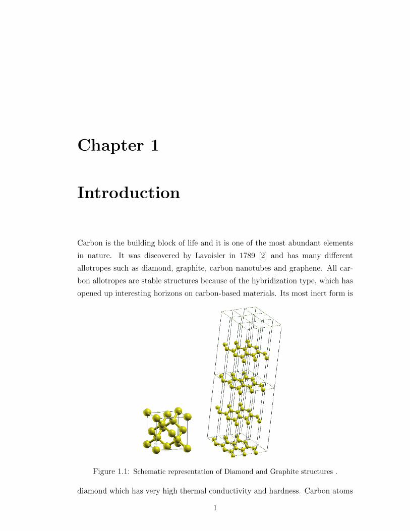
Carbon is the building block of life and it is one of the most abundant elements

in nature. It was discovered by Lavoisier in 1789 [2] and has many different

allotropes such as diamond, graphite, carbon nanotubes and graphene. All car-

bon allotropes are stable structures because of the hybridization type, which has

opened up interesting horizons on carbon-based materials. Its most inert form is

Figure 1.1: Schematic representation of Diamond and Graphite structures .

diamond which has very high thermal conductivity and hardness. Carbon atoms

1

in diamond structure make tetrahedral bonds. It is an insulating material with

a large band gap. It transmits all the spectrum of light which makes it very

valuable material in industrial applications.

Graphite is another important carbon structure. Layers of carbon atoms are

stacked on each other forming three dimensional structure. These layers are held

together by weak van der Waals forces. One of the very first studies of graphite

structure is by B.T Kelly in 1981. [3] In this study, the elastic properties of

graphite have been reviewed, displacement and irradiation effects of atoms in the

graphite structure have been studied in detail.

After the discovery of graphite, it was believed that fabrication of monolayer

graphite structure is not possible due to the thermal instability. However, the

material called ”graphene” was exfoliated in 2004 by Geim and K.S. Novoselov

[4, 5]. This monolayer structure has amazing properties and lead researchers

to work in quantum relativistic effects and low dimensional physics despite its

short history of syntesis. However, this structure is chemically inert and in order

to make this material chemically active different approaches have been tried at

different levels of sophistication.

Adatom adsorption is a method to make graphene active and has become

very popular over the last few years. The primary goal of this thesis is to study

theoretically adatom and dimer adsorption on graphene. To this aim, we have

investigated structural properties of several atoms and dimers.

This thesis is composed from four chapters. In this chapter, the basics of

graphene crystal structure and its place in condensed matter world have been

briefly reviewed. Moreover, the important studies on graphene in the scope of

tailoring electronic and structural properties have been summarized. The fol-

lowing chapter covers theoretical background of Density Functional Theory (the

schemes and approximations that we have used are also explained). Chapter 3

and 4 present the calculations, results and concluding remarks, respectively. Fi-

nally, a brief discussion on Quantum Espresso Package [6] is included at the end

of the thesis.

2

1.0.1 The Graphene Structure

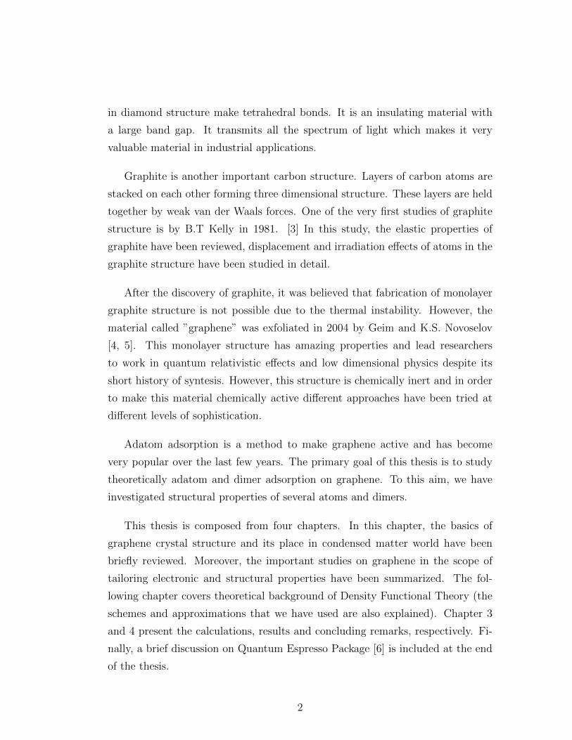
Graphene is a two dimensional, one carbon-atom thick material with each C atom

forming three bonds with each of its nearest neighbors. It can be considered

as a building block of carbon materials of other dimensionalities such as the

0 dimensional bucky ball, 1 dimensional carbon nanotubes and 3 dimensional

graphite. It has become very popular over the last few years because it represents

Figure 1.2: Schematic representation of single layer graphene .

new type of material which offers a strong ground for applications. [7]

Graphene is the first two-dimensional material with high crystal quality. It

was believed that two dimensional materials are thermodynamically unstable and

thus can not be used in applications. However, the soft crumbling in the third

dimension in graphite made it possible to fabricate this structure.

Graphene has a honeycomb lattice, as shown in figure 1.3 with lattice vectors

in real space are given by

a1 =a√

3

2x+

a

2y (1.1)

a2 =a√

3

2x− a

2y (1.2)

where a =√

3acc and acc = 1.42 Angstrom is the carbon-carbon distance in

3

a1

a2

Figure 1.3: Crystal structure of single layer graphene .

graphene. Reciprocal lattice vectors in momentum space are given by

b1 =b

2x+

b√

3

2y (1.3)

b2 =b

2x− b

√3

2y (1.4)

where b = 4πa√3.

In contrast to diamond, the carbon atoms in graphitic materials are sp2 hy-

bridized. Carbon has four valence orbitals (2s,2px,2py, 2pz). Graphene sheet

is formed when s, px and py orbitals are combined forming σ(bonding) and σ∗

(antibondig) orbitals. The remaining pz orbital extends along the z direction on

the graphene sheet. The interaction among pz orbitals creates the delocalized π

(bonding) and π∗ (antibonding) orbitals [8, 9]. Graphene consists of covalently

bonded carbon atoms and this strong binding comes from the σ bonds. However,

the fourth valence electron does not contribute to the covalent bond, instead

these pz orbitals form weakly interacting graphene layers. The high symmetry

points of the reciprocal space and the band structure for graphene are shown in

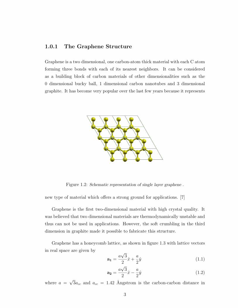
Figure 1.4 and 1.5 respectively. At low temperatures, cosine like energy band

is linear, E = hvFk, and therefore, it also has linear dependence of density of

states at the K point. At the edge of the Brillouin zone, these two linearly dis-

persing bands touch each other. That is called Dirac point and electrons and

4

Figure 1.4: High symmetry points G,K,M in reciprocal space .

holes at the corners of the Brillouin zone have zero effective mass and these are

called massless Dirac fermions. This reduction in mass of the fermions is caused

by the interaction with the periodic potential of honeycomb lattice. It has the

honeycomb shape lattice with two equivalent carbon sublattices. Since each of

two sublattices should contribute as two different wavefunctions at Dirac points,

they are known as pseudospin and shown by σ in Dirac Hamiltonian [7]

H = hvF

0 kx − ikykx + iky 0

= hvF~σ · ~k (1.5)

where ~k is the quasiparticle particle, ~σ is the 2D Pauli matrix, vF plays the role of

speed of light. They are 1/2 spin particles (fermions). Moreover, these particles

have very high mobility, they have velocity of an effective speed of light (vF = 106

m/s) and it is independent of temperature between 10 to 100 K. These charge

carriers can travel thousands of interatomic distance before colliding.

This exceptional property of high mobility gives rise to the anomalous quan-

tum Hall effect when they are exposed to magnetic field at high temperatures.

Underlying theory of Hall effect is as follows. When the electric current is flowing

in the wire in the x direction and a magnetic field Bz applied normal to the wire

in the z direction. An additional electric field normal to both of these fields is

created. Hall conductivity is given by σ = ν e2

h. where ν is the filling factor and

depending on this constant (integer or fractional) Hall effect is named as inte-

ger quantum Hall effect or fractional Hall effect and Hall constant for electron

5

−20

−15

−10

−5

0

5

10

Energ

y (

eV

)

Γ K M K 1 2

DOS(electron/eV)

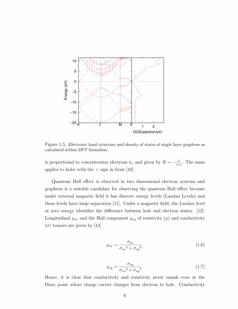
Figure 1.5: Electronic band structure and density of states of single layer graphene ascalculated within DFT formalism.

is propertional to concentration electrons ne and given by R = − 1nee

. The same

applies to holes with the + sign in front [10].

Quantum Hall effect is observed in two dimensional electron systems and

graphene is a suitable candidate for observing the quantum Hall effect because

under external magnetic field it has discrete energy levels (Landau Levels) and

these levels have large separation [11]. Under a magnetic field, the Landau level

at zero energy identifies the difference between hole and electron states. [12].

Longitudinal ρxx and the Hall component ρxy of resistivity (ρ) and conductivity

(σ) tensors are given by [12]

ρxx =σxx

σxx2 + σxy2(1.6)

ρxy =σxy

σxx2 + σxy2(1.7)

Hence, it is clear that conductivity and resistivity never vanish even at the

Dirac point where charge carrier changes from electron to hole. Conductivity

6

for graphene is given by [7]

σxy =±4e2

h(N +

1

2) (1.8)

where N denotes the Landau level and 4 comes from the double spin degeneracy.

This explains pretty well that graphene’s conductivity tensor exhibits neither

standard quantum Hall Effect nor fractional Hall effect. It exhibits anomolous

quantum Hall effect.

Another very interesting feature of graphene is that it has minimum con-

ductivity and zero resistivity. Since it is a zero band gap semiconductor, the

resistivity change is almost zero.

From an experimental point of view, it is not useful for device applications.

Indeed, introducing a band gap is an important step to overcome this difficulty.

Last but not least, graphene’s extraordinary unique features are promising for

electronics and photonics. Its charge carriers have unique features. Further,

perhaps even greater their mobility remains the same under ambient conditions

e.g. by changing electronic structure, by exposing to magnetic field, by doping

etc. Therefore, graphene can be used as a transistors. Low switching time is

important in order a transistor to be more efficient. Graphenes low resistance

contacts is another advantage to reduce the switching time. It might be possible

to introduce transistors at THz frequency range by the graphene based electronics

[7].

7

1.0.2 Tailoring Structural and Electronic properties of

Graphene

In this section, various theoretical studies will be addressed on tailoring the elec-

tronic structure of graphene. There are many different ways to change the crys-

tallographic structure of graphene. In order for graphene to be used in future

electronic devices, the Fermi level should be tuned to change graphene from

metal to semiconductor. In other words, the band gap should be controllable in

this stable and relatively inert material.

One of the most important ways of changing the electronic structure of

graphene is doping which can be investigated by changing the number of elec-

trons of the system. Doping can be obtained by several methods such as taking

the advantage of supporting substrate, by means of external internal stress and

adsorption of proper donors or acceptors.

Graphene on different substrates have been investigated by numerous works.

Especially, intercalation of layer of atoms between graphene and its host has been

studied in various works. Silicon carbide is one of the most common materials

used as a host because graphene grows nearly decoupled from silicon carbide

substrate [13]. Then, intercalation by different atoms gives rise the change in the

work function due to doping. In a recent study by Sandin et al. [13] ab initio

calculations have been performed for different intercalation structures for Na in

graphene on SiC substrate. They showed that Na electron dopes the graphene and

it intercalates in between graphene layer and silicon carbide substrate. In fact,

when graphene is grown on the silicon face of this substrate leading to formation

of monolayer graphene covalently bonded to the substrate (buffer layer), graphene

becomes insulator with a large band gap. However, when they adsorbed Na atoms

between the buffer layer and substrate, electron doping was found to increase and

work function decreased accordingly. On the other hand, when the Na atom was

placed in between the graphene layer and the SiC substrate they observed a shift

of the Dirac point but the linear behavior of band structure was observed to

remain the same.

8

The role of the covalent and metallic intercalation of graphene on SiC sub-

strate has been studied by many other scientists. Deretzis et al. [14] presented a

density functional theory study of hydrogen and lithium intercalation of graphene

on SiC substrate. They showed that hydrogen and lithium adsorption causes the

buffer layer to be detached from the silicon carbide surface. Hydrogen intercala-

tion gives rise minimal perturbation at the Dirac point while lithium intercalation

creates the highly n-doped system with the Dirac cone to shift to the valence band

of SiC substrate.

Another hydrogen intercalation study of graphene on SiC substrate is by

Hiebel et al. [15] and Boukhvalov [16]. They have performed density functional

theory calculation for epitaxial graphene on SiC. Boukhvalov observed a small

band gap opening by hydrogenization and fluorination of graphene on SiC.

The main goal of these studies is to decrease the strong interaction between

buffer layer and SiC. Since it has been shown that first C layer (buffer layer)

on SiC displays graphene like structure, intercalation by atoms would lead to

electronic structure modification.

Yet another group, Garces et al. [17] have pointed out the importance of

dielectric material on graphene-based technologies. Although, it is known to be

a challenge to deposit dielectric oxide on graphene due to the inert nature of

graphene, it enhances the overall graphene device performance.

Dedkov et al. [18] studied iron layer intercalation between graphene and nickel

(111) surface. Voloshina et al [19] have also performed electronic structure cal-

culations to investigate the properties of graphene on ferromagnetic substrate by

intercalating metal. They calculated adsorption energy of several systems such

as graphene on top of Ni(111) surface, graphene on top of Al (111) surface and

intercalation of aluminium layer between graphene and Ni(111) surface. Com-

paring the results, graphene on nickel surface seems to be more stable than the

others. Since Ni is a 3d metal, hybridization is observed between graphene’s π

and nickel’s d states. This interaction has then changed the electronic structure

of graphene considerably. It causes shift of graphene’s band to higher energies.

Graphene on the Ni substrate with aluminium layer intercalation on the other

9

hand still gives the Dirac point. This system doesn’t deviate from the normal

electronic structure properties of the graphene layer. Using a metallic substrate

without intercalation of any other atom is another promising way in integrated

electronics. Xu et al. [20] studied the interface structure between graphene and

copper (111) and nickel (111) surface. They showed that nickel has much larger

cohesive energy than copper. That is due to the strong interaction between open

d-orbitals. Andrew et al. [21] used crystal copper surface (111), (100) and on

both substrate graphene was caused to the shift of Dirac crossing and to open

bandgap.

Besides using different kind of materials as a host, there are numerous studies

of intrinsic defects on graphene. There are different types of defects such as inter-

sitial defects, vacancy defects, Stone-Wales defects [22]. Li et al. [23] emphasized

the importance of the vacancy on graphene as a simplest intrinsic defect. They

performed ab initio calculations to study defect formation energies. In literature,

there are numerous studies on alkaline earth metals on graphene as a hydrogen

storage material because they are believed to be very strong adatoms since bulk

cohesive energy is quite weak therefore they do not cluster on top of graphene.

Thus, Hussain et al. [24] have choosen calcium atoms as a dopant for hydro-

gen storage on graphene. They concluded that binding energy of Ca atoms on

graphene is higher than its bulk cohesive energy resulting in the stability of the

calcium doped graphene system. On the other hand, band structure of graphene

can also be tailored by doping. Attaccalite et al. [25] have already investigated

that for high concentrations of dopants, linearity of bands at Dirac points is bro-

ken. In addition to this, they have also estimated that Fermi velocity is also

altered by doping. Further, Wu et al [26] introduced different configurations

of vacancies in hydrogenated graphene and fluorinated graphene. The resulting

structure is chain-like vacancy in both hydrogenated and fluorinated graphene.

The importance of the stress and strain on graphene structure calculations

has been pointed out by different groups. In order to transform this inert layer in

to a chemically active one, Andres et al. [27] studied the effect of tensile stress on

σ and π bonds. By performing ab initio study of hydrogen on large clusters and

periodic graphene structure. They concluded that stess affects π bonds giving rise

10

to more strong binding to the adsorbed atoms. Wen et al [28] studied graphene

crystals over a wide pressure range. They realized that band gap width increases

linearly with pressure however, band gap slightly decreases at very high pressures.

It is stated that stability of structure is correlated with the band gap i.e. less

stable structures have smaller gaps. Thus, graphene crystals are not very stable

at very high pressures e.g., 300GPa.

11

1.0.3 A Brief Survey of the Atomic and Molecular Ad-

sorption on Graphene

Many theoretical studies have been performed in order to understand the in-

teraction between graphene and adsorbed atoms. Researchers have investigated

several important schemes to find stable configurations and have reported im-

portant properties of these systems such as charge transfer between adatom and

graphene, work function difference in the energy band diagram. The main goal

of these works is to change hybridization from sp2 to sp3. When the adatom is

adsorbed on graphene, the additional electron is localized on pz like orbital thus

is a suitable candidate to form covalent bond along z direction. On the other

hand, in-plane carbon-carbon bond becomes longer and weakened by keeping the

same crystal structure. That means that the structure is on the way to become

sp3 hybridized structure giving rise to opening a bandgap. [27]

In the pioneering work by Sofo et al. [29], it has been predicted that hy-

drogen can be adsorbed on graphene. This structure is called ”graphane” and

the stability of this structure has also been verified experimentally by Elias et

al. [30]. In this structure, each carbon atom binds to an additional hydrogen

thus changes the structural and electronic properties of the whole system. The

resulting stable structures are chair-like and boat-like configurations of graphane.

Chair configuration is hydrogen atoms alternating on both sides of graphene and

boat like configurations is hydrogen atoms alternating on both sides of graphene

in pairs. They obtained the carbon-carbon distance value as 1.52 A. Boat-like

Figure 1.6: Chair configuration hydrogenated graphene.

12

Figure 1.7: Boat configuration hydrogenated graphene.

configuration on the other hand, has two different C-C bond length depending

on the H-H distance. For both of these structures the C-H distance is 1.1 A,

which complies with those found in literature. The chair configuration is more

stable than the boat configuration. On the other hand, they revealed that boat

and chair conformers show semiconducting behavior with band gaps very close to

each other, (3.5 eV and 3.7 eV respectively). Charge density analysis shows that

charge transfers are from hydrogen to carbon atom. Phonon calculations show

that boat configuration has higher frequency than chair one, because of the closer

distance of first nearest neighbor hydrogen atoms in boatlike structure. Last but

not least, they found chair-like graphane as stable as fluorographene which is the

most stable structure in halogen atom adsorption on graphene and graphane is

even more stable than graphite and other hydrocarbons such as cyclohexane ben-

zene etc. Although, graphane has a large band gap which makes this structure

inappropriate for the applications, hydrogen doping might be a good starting

point to tune the bandgap and the density of charge carriers in conduction band.

Following this study, a year later, it was theoretically verified by Boukhvalov

et al [31] that the chair-like configuration of graphane is the most favorable struc-

ture. The chemisorption energy as a function of hydrogen concentration was cal-

culated. The chair-like conformer was found to experience vertical buckling with

around 0.45 A which complies with the experimental buckling value of graphane

by Elias et al. [30] C-H bond length is around 1.2 A which is consistent with the

results of Sofo et al. [29].

Strain engineering on reversible hydrogenation of graphene has been suggested

13

by Pereira et al. [32]. Boat and chair configurations with symmetric and anti-

symmetric structures were considered. The results show that the antisymmetric

configuration is energetically more stable. Symmetric configurations displays the

sp2 hybridization of graphene with a band gap of 0.26 eV whereas the antisym-

metric configuration gives the value of 3.35 eV for the band gap.

Stability of halogens (F, Cl, Br, I) on graphene have been also studied by

Medeiros et al. [33]. The graphane structure was also studied for comparison

purposes. It was concluded that the chair configuration of graphane is less stable

than fluorinated graphene.

Following this, numerous possible configurations of hydrogenated graphene

and fluorinated graphene structures has been studied by Leenaerts et al. [34]. The

results show that the chair configuration of graphane is the most stable structure.

In addition to the chair configuration, boat, zigzag and armchair configurations

have also been investigated in detail. It is clear that zigzag configuration which

has not been studied before Leenaerts et al. is found to be more stable than boat

and armchair configurations. The resulting structural and electronic properties

of graphane shows that the charge transfer between hydrogen and carbon is very

small due to the similar electron affinity of these atoms. Further, band gap value

is found to be 3.70 eV for chair graphane.

The comparative analysis of fluorinated and hydronated graphene structures

have been performed by Sahin et al [35]. Chair configuration of hydrogenated

graphene is less stable than fluorinated graphene as in the previously mentioned

studies. They have also worked on different decorations of flourine atoms on

graphene which is going to be investigated in detail below.

Different than previously held concepts of graphane, nature of single sided

hydrogenated graphene has been studied by Subrahmanyam et al. [36]. Different

concentration with different initial distance of hydrogens at different coverages

on graphene have been studied. Consistent with experimental observations, their

results indicate that 50 percent coverage gives the most stable structure. For

comparison purposes with the other data in table 1, only full coverage with initial

hydrogen-carbon distance less than 1.2 A will be displayed in table 1.

14

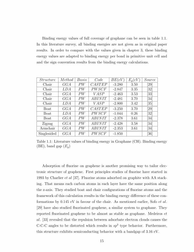
Binding energy values of full coverage of graphane can be seen in table 1.1.

In this literature survey, all binding energies are not given as in original paper

results. In order to compare with the values given in chapter 3, these binding

energy values are adapted to binding energy per bond in primitive unit cell and

and the sign convention results from the binding energy calculations.

Structure Method Basis Code BE(eV ) Eg(eV ) SourceChair GGA PW CASTEP -3.280 3.50 [29]Chair LDA PW PWSCF -2.847 3.35 [32]Chair GGA PW V ASP -2.463 3.53 [33]Chair GGA PW ABINIT -2.481 3.70 [34]Chair LDA PW V ASP -2.800 3.42 [35]

Boat GGA PW CASTEP -3.250 3.70 [29]Boat LDA PW PWSCF -1.044 0.26 [32]Boat GGA PW ABINIT -2.378 3.61 [34]

Zigzag GGA PW ABINIT -2.428 3.58 [34]Armchair GGA PW ABINIT -2.353 3.61 [34]

Singlesided GGA PW PWSCF -1.850 [36]

Table 1.1: Literature values of binding energy in Graphane (CH). Binding energy(BE), band gap (Eg)

Adsorption of fluorine on graphene is another promising way to tailor elec-

tronic structure of graphene. First principles studies of fluorine have started in

1993 by Charlier et al [37]. Fluorine atoms adsorbed on graphite with AA stack-

ing. That means each carbon atoms in each layer have the same position along

the z-axis. They studied boat and chair configurations of fluorine atoms and the

framework of this calculation results in the binding energy difference of these con-

formations by 0.145 eV in favour of the chair. As mentioned earlier, Sofo et al.

[29] have also studied fluorinated graphene, a similar system to graphane. They

reported fluorinated graphene to be almost as stable as graphane. Medeiros et

al. [33] revealed that the repulsion between adsorbate electron clouds causes the

C-C-C angles to be distorted which results in sp3 type behavior. Furthermore,

this structure exhibits semiconducting behavior with a bandgap of 3.16 eV.

15

A comparative study of graphane and fluorinated graphene have been per-

formed by Leenaerts et al. [34]. Stability analysis of structures shows that the

zigzag configuration is more stable than boat and armchair configurations. The

calculations show that boat and chair conformations have high Young modu-

lus which makes these structures quite strong. Overall, the result of this study

shows larger values compared to the previously performed experimental works,

however, they attribute the reason to the nature of defects in the samples used

in experimental studies.

The scope of carbonmonofluoride and graphane has also been investigated by

Artyukhov et al. [38]. As in the study of Leenaerts et al. [34], three different

conformations e.g chair boat and zigzag or armchair conformations have been

studied which was called chair, bed and washboard or gauche chair, respectively.

To avoid confusion, it is referred as the usual names here. For both fluorographene

and hydrogenated graphene, armchair configuration turned out to be more stable

than zigzag and boat configurations. Considering chair configuration as a refer-

ence energy, fluorinated graphene armchair and boat configurations have 0.071

eV and 0.148 eV respective energies per primitive unit cell . In hydrogenated

graphene on the other hand, armchair and boat configurations have 0.055 eV and

0.103 eV energies with respect to chair one. The difference between fluorinated

graphene and hydrogenated graphene is that fluorinated graphene conformations

longer carbon carbon distance in optimized structures because of more electron

cloud repulsion in this. Further, C-H and C-F distances are 1.112 A and 1.382 A

respectively, which in turn leads the approval of previous studies.

In another work, Samarakoon et al [39] first principles density functional

theory calculations have been performed to understand electronic and structural

properties of fluorographene and graphane. They studied so called chair, boat,

stirrup and twist boat configurations. Stirrup conformation is such that fluorine

atoms alternates on both sides of zigzag direction of carbon atoms whereas in

the twist boat configurations are atoms alternates only in zigzag or armchair

direction. Comparing these structures, chair configuration is the most stable one,

indeed, it is consistent with the other studies. Stirrup conformation is even more

stable than boat and twistboat conformation. Fluorinated graphene found to be

16

more stable than graphane. All the binding energies are in very good agreement

with the study of Leeanerts et al. [34]. Band gap values are 3.1 eV for the chair

conformation and 3.5 eV for the stirrup configurations which are also similar with

the previously held experimental and density functional theory based studies.

It has been revealed by Sahin et al. [35] that the fluorine atom coverage effects

the important properties of the structure. It was found that C4F , C2F boat, C2F

chair, CF chair conformations are stable. The important point here is that some

of the optimized structures might results in unstable structures such as CF boat

conformation. They performed this particular calculations by density functional

perturbation theory. Although band gap of the fluorinated graphene structures

are ranging from 69 meV to 3 eV, GW0 approximations have been carried out to

correct the gap value because density functional theory calculations is known to

underestimate gap values. Hence, CF structure with band gap of 7.49 eV which

is in fact a way too large compared to DFT calculation result. However, apply-

ing strain to the system results in reduction of band gap value. On the other

hand C2F chair structure exhibits metallic behavior which can be the reason of

odd number of electrons in the primitive unit cell. There are several methods to

analyze charge transfer. In order to obtain the accurate results with the method

they use, they subtract charge density of isolated carbon and fluorine atoms from

the resulting value. The resulting charge transfer is from the middle of C-C bond

and to F atom. This is a reasonable result considering the electronegativity of

fluorine atom compared to carbon atom. Moreover, fully covered chair configu-

ration is nonmagnetic system however, upon vacancy with a single fluorine atom,

a magnetic moment in the system is created because of the unpaired π orbitals

of that single fluorine atom. This study suggest that concentration of fluorine

atom change gives rise to the creation of different structures and some external

applications leads possibility to change electronic and elastic properties.

In the experimental side of this work, the very first study of fully covered

fluorinated graphene studied by Nair et al [40], it has been suggested that fluo-

rinated graphene has bandgap of 3 eV and another work by Robinson et al [41]

have revealed that single side adsoption creates large band gap at different con-

centration of flourine atoms on graphene. Recent study by Kwon et al. [42] shows

17

that fluorination on graphene tailor adhesion, friction and charge transport prop-

erties of graphene. Friction on graphene is known to arise from flexural phonons,

thus functionalization of graphene increases friction. Furthermore, their result

revealed that fluorinated graphene has 2.9 eV bandgap which also complies with

the theoretical calculation results. In order to verify the experimental results,

density functional theory calculation has been performed. They have approved

the possibility of single sided fluorination by 25 percent fluorination. Full cover-

age of fluorine atoms on the other hand, gives that the chair like conformation is

the most stable structure. Elastic properties of graphene e.g bending and stiffness

constants which is not going to be discussed here in detail, however, calculations

result in the increase of frictional forces with fluorination process and that is all

about the bending and stiffness constants. Cheng et al. [43] showed that through

the reduction process of multilayer fluorinated graphene, it is possible to produce

conductive material which might be a milestone for fluorine adsroption based

graphene and its applications.

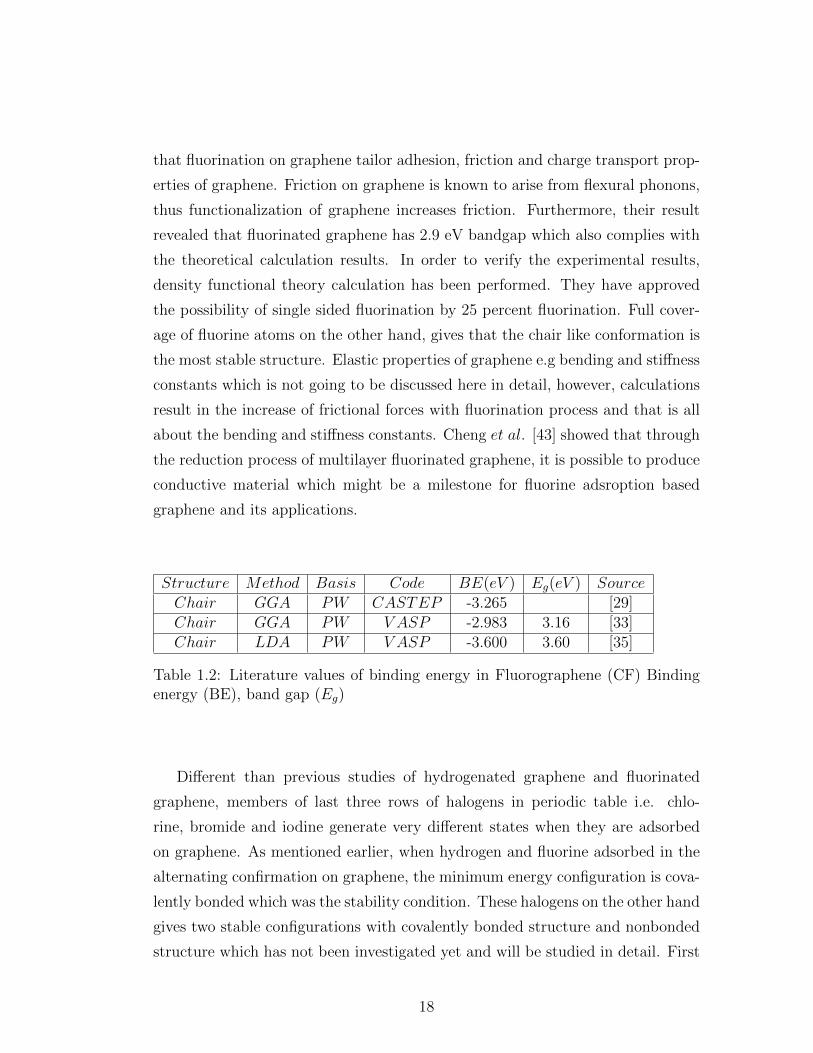
Structure Method Basis Code BE(eV ) Eg(eV ) SourceChair GGA PW CASTEP -3.265 [29]Chair GGA PW V ASP -2.983 3.16 [33]Chair LDA PW V ASP -3.600 3.60 [35]

Table 1.2: Literature values of binding energy in Fluorographene (CF) Bindingenergy (BE), band gap (Eg)

Different than previous studies of hydrogenated graphene and fluorinated

graphene, members of last three rows of halogens in periodic table i.e. chlo-

rine, bromide and iodine generate very different states when they are adsorbed

on graphene. As mentioned earlier, when hydrogen and fluorine adsorbed in the

alternating confirmation on graphene, the minimum energy configuration is cova-

lently bonded which was the stability condition. These halogens on the other hand

gives two stable configurations with covalently bonded structure and nonbonded

structure which has not been investigated yet and will be studied in detail. First

18

of all, different configurations of halogen atoms on graphene in addition to cova-

lently bonded fluorinated graphene and graphane have been studied by Medeiros

et al. [33] There are two different configurations as bonded and nonbonded for

chlorine, bromide and iodine atoms. Indeed, bonded configuration is not dif-

ferent from fluorinated and hydrogenated graphene whereas in the nonbonded

configuration, van der Waals type interaction play an important role. The struc-

tural properties of nonbonded system is indeed different than the bonded system.

Lattice parameter of nonbonded system is closer than those of bonded system.

Increase interaction between carbon atoms with smaller lattice parameter makes

corresponding carbon-adsorbate atoms weak enough which tends to behave as

van der Waals type interaction. Also, the repulsion between adsorbate atoms

which are close to each other, forces adatoms to go away. Further, when the

repulsion is compansated by the weak van der waals interactions, adatom find its

equilibrium. Therefore, exchange correlation potential should be approximated

by van der waals density functional theory instead of local density functional the-

ory. Comparing the structural properties of all systems, they revealed that as the

atomic radius increases C-C-C angles also increases. In the electronic structure

part of the study, it is found that charge transfer depends on halogen polarizabil-

ity. Since bromide and iodine have higher polarizability charge transfer direction

is not the same with the direction of fluorine and chlorine. Another study by Di

et al. [44] has also investigated graphane like structures i.e. fluorine, chlorine and

bromide on graphene. They have calculated chair configuration of these atoms

with the full coverage of graphene, the results are shown in table 1.3

Very recent studies in the scope of chlorination performed by Yang et al.

[45], Ijas et al. [46] and Sahin et al. [47]. Yang et al. [45]. The results in single

atom adsorption are shown in table 1.6. Different concentration of chlorine atoms

on graphene have also been studied. Unlike hydrogenization, it was found that

Cl adatom has two configurations for the full coverage, bonded and nonbonded.

Nonbonded configuration is energetically more favorable than bonded configura-

tion which has covalent interaction between them. Double sided chlorination is

even more stable than single sided chlorination. Further, single sided 25 percent

coverage is the most stable with the binding energy of -1.61 eV.

19

Atom− Structure Method Basis Code BE(eV ) Eg(eV ) SourceCl −Nonbonded GGA PW V ASP -0.669 - [33]Cl −Bonded -0.066 1.53

Br −Nonbonded GGA PW V ASP -0.080 - [33]Br −Bonded 1.255 -I −Nonbonded GGA PW V ASP 1.265 - [33]I −Bonded 2.500 -

Cl −Bonded GGA PW CASTEP 2.463 1.66 [44]Br −Bonded GGA PW CASTEP 2.108 - [44]

Table 1.3: Literature values of binding energy of halogens on graphene. Bindingenergy (BE), band gap (Eg)

Dimer Structure C-dimer Distance Binding energy(eV)F2 Bridge 3.47 -0.214

Hollow 3.70 -0.187Top 3.46 -0.218

Cl2 Bridge 4.21 -0.208Hollow 4.34 -0.193Top 4.21 -0.210

Br2 Bridge 4.51 -0.229Hollow 4.67 -0.207Top 4.45 -0.214

I2 Bridge 4.74 -0.375Hollow 4.85 -0.352Top 4.73 -0.379

Table 1.4: Halogen dimers in perpendicular-to-plane configurations

There are two types of adsorption on graphene. The modes of these adsorption

types are known as physisorption and chemisorption. In the case of chemisorption,

the nature of bond is covalent or ionic at some level. On the other hand, if the

case is physisorption, a weak interaction between adsorbate and graphene takes

place. So far, we have reviewed local density functional theory studies which

are all about the adsorbates strongly bound on graphene. There is no strong

interaction between adsorbate atoms, however if there is any covalently bonded

molecules adsorbed on graphene, the structure and its approximation for the

exchange correlation potential changes considerably. Local and semilocal density

functional theory approximation will have no success to understand such weak

behavior between adsorbates and graphene. Hence, a new approximation called

20

Dimer Structure C-dimer Distance Binding energy(eV)F2 Bridge 3.17 -0.231

Hollow − alongx 3.23 -0.227Hollow − alongy 3.24 -0.225

Hollow − along√32x 3.23 -0.226

Bridge− alongy 3.26 -0.222Cl2 Bridge 3.58 -0.259



Bridge− alongy 3.63 -0.251Br2 Bridge 3.74 -0.296



Bridge− alongy 3.78 -0.288I2 Bridge 3.80 -0.523



Bridge− alongy 3.81 -0.512

Table 1.5: Halogen dimers in in-plane configurations

van der Waals density functional approach is needed. Further description in this

theory can be seen in chapter 2.

21

In this purpose, adsorption of halogen dimers on graphene has been studied

by Rudenko et al. [48]. In-plane bridge configuration is the most stable whereas

binding energy decreases by increasing the distance of dimer and graphene. How-

ever, fluorine dimer at large distances has inversely proportional behavior which

shows that this structure has ionic bonding as well. That means that even at

large distances electron density might overlap between that of graphene without

any need to the van der Waals term. The investigation by only generalized gra-

dient approximation for fluorine dimer also approves the idea that in the absence

of van der Waals term, fluorine dimer has still interaction with graphene. Charge

transfer analysis also complies with this result. Considerable amount of charge

transfer to fluorine dimer is present, it accepts electrons more than iodine and

bromide dimer. The corresponding binding energy and relevant distances are

shown in table 1.4-1.5. It is clear that there are not so much difference in bind-

ing energy of such configurations for in-plane configurations and perpendicular

to plane configurations altough the binding energy in-plane and perpendicular to

plane configurations differ.

Atom Site Method Basis Code BE(eV )/atom SourceF TOP GGA PW CASTEP 2.273 [44]F BRIDGE 1.906F HOLLOW 2.046Cl TOP GGA PW CASTEP 1.025 [44]Cl BRIDGE 1.024Cl HOLLOW 1.021Br TOP GGA PW CASTEP 0.769 [44]Br BRIDGE 0.767Br HOLLOW 0.764

Cl TOP LDA PW V ASP -1.130 [45]Cl TOP GGA -0.880F TOP LDA PW V ASP -2.570 [45]

Cl TOP V DW −DF PW FHI − aims -1.212 [46]Cl BRIDGE -1.210Cl HOLLOW -1.196

Table 1.6: Literature values of binding energy of single halogens at differentpositions. Binding energy (BE)

22

Until now, we have made literature survey on the full coverage and dimer ad-

sorption on graphene. Another possibility in adsorbed graphene studies is surely

to investigate how the single adatom tailor the bonding and structural proper-

ties of graphene. For this purpose Di et al. [44] changed adatom concentration

to understand stable configurations. When there is only one adatom is present,

fluorinated graphene is the only chemisorbed structure while chlorinated and bro-

mide structures may only be chemisorbed by full coverage due to adsorbed atom

interaction. They tried different high symmetry sites for single flourine adatom

to find its stable position. This is the top side position which gives the smallest

fluorine-graphene distance. In the charge density analysis, the charge density

overlap has been investigated in fluorine system whereas bromide and iodine has

a little overlap in the charge density. Chlorine and bromide adatom exhibits sim-

ilar adsorption energies. The resulting adsorption energies can be seen in table

1.6.

Amongst the most recent works, one of the noteworthy studies is by Yang et

al. [45]. The resulting binding energy comparison exhibits that Cl atom prefers

top position with 2.53 A C-Cl distance. They have also performed for single

F and H atoms adsorption for comparison purposes. Ijas et al. [46] found top

position most stable one. In the same way, Sahin et al. [47] have also found top

position of single Chlorine adatom with the binding energy of 1.16 eV by van der

Waals correction. The results are summerized in table 1.6.

23

Chapter 2

Methodology

2.0.4 Density Functional Theory

Since the 1970’s, Density Functional Theory (DFT) has been extensively used for

the study of the electronic structure of atoms, molecules and solids, usually with

very good agreement with experimental data and in many cases, with relatively

low computational cost when compared to other more elaborate methods within

many-body theory. The formalism is based on the Hohenberg-Kohn theorem

which states that the ground-state energy of the system can be expressed as

a functional of the ground-state single-particle density. The theorem, however,

does not provide the form of this universal functional, which is unknown and,

therefore, approximations have to be made. Within DFT one writes the total

energy of the interacting system as a sum of different terms:

E[n] = T [n] +∫Vion(r)n(r) d 3r +

1

2

∫ n(r)n(r′)

|r− r′|d 3r d 3r′ + Exc[n(r)] . (2.1)

Here, T [n] is the kinetic energy of a non-interacting system with the same den-

sity n as the fully interacting system, Vion(r) is the electron-ion potential. The

third term represents the Coulomb interaction and the term Exc[n] represents the

remaining contribution to the total energy. That is the part whose exact form

is unknown and which has to be approximated. The first term, kinetic energy is

24

written as

T [n] = −1

2

∑i

∫ϕi∇ 2 ϕ∗i d

3r (2.2)

The most popular approach within DFT is that due to Kohn and Sham (Kohn-

Sham DFT). Here, the problem of a system of interacting electrons is reduced

to problem of non-interacting electrons moving in an effective potential which

includes the effects of the Coulomb interaction between the electrons. In this

approach, the non-interacting energy is calculated exactly from the one-electron

orbitals obtained from a set of one-electron Schrodinger-like equations in which

the effects of exchange and correlation between the electrons appear in an effective

but local one-electron potential. Suppose that we have a number N of non-

interacting electrons subject to an external potential. The wave function ϕk(r)

of these electrons are then obtained from the Kohn-Sham equation. [1](−1

2∇ 2 + Vion(r) + VH(r) + VXC(r)

)ϕi(r) = εi ϕi(r) , (2.3)

where VH(r) is the Hartree potential and given by

VH(r) =1

2

∫ n(r′)

|r− r′|d 3r′ . (2.4)

and exchange-correlation potential, VXC(r) is given by the functional derivative;

VXC(r) =δEXC [n(r)]

δn(r)(2.5)

According to Pauli exclusion principle only one electron is allowed to occupy any

single orbital or at most two electrons if we consider spin. We can thus have one

spin-up electron and one spin-down electron in every orbital. When we solve this

potential, we realize that the lowest total energy is obtained, i.e, the ground state

energy, if we put the electrons in the orbitals with the smallest eigenvalues, of

course taking due account of the Pauli exclusion principle. This is referred to as

the aufbau principle. The total particle density of the N electron system is just

the sum of the individual densities |ϕi(r)|2 of every electron. Thus,

n(r) = 2∑i

|ϕi(r)|2 . (2.6)

where factor 2 comes from spin states. Moreover, Hohenberg and Kohn showed

that the functional for the total energy is minimized by the correct ground-state

25

density pertinent to the potential V (r) . When we change the external poten-

tial V (r) every single orbital being a solution to the Kohn Sham equation will

also change. Thus, the density will change too. We can then hope to find an

external potential V (r), called the Kohn-Sham potential, such that the particle

density becomes identical to the particle density of a fully interacting system of

N electrons. One can show that there is a unique potential which yields the exact

interacting one-electron density of the system when it is calculated as the sum of

the squares of the one-electron orbitals - one for each electron of the system.

The most difficult problem in electronic structure calculations is to deal with

electron-electron interactions. Electrons with the same spin should be spatially

separated and it reduces the Coulomb energy. This is called exchange energy and

it is solved by Hartree-Fock approximation. Furthermore, electrons with oppo-

site spins also repel each other due to Coulomb interactions. Thus, the coulomb

energy is reduced at the cost of increasing kinetic energy. The difference between

many body energy and calculated Hartree-Fock energy is called correlation en-

ergy [1]. The simplest approach to describe exchange-correlation energy is the

local-density approximation (LDA) in which the exchange-correlation part of the

potential is taken to be the exchange-correlation contribution to the chemical

potential of the homogenoeus but interacting electron gas of a density equal to

the local density of the inhomogeneous system. The exchange correlation energy

of the inhomogeneous system is calculated by dividing the system into pieces so

small that the density in each piece can be considered to be constant and equal to

the local density of the inhomogeneous system at that point. The total exchange-

correlation energy of the inhomogeneous system is then obtained as the sum of

the exchange-correlation energies of these homogenous pieces. Thus,

EXC [n] =∫εxc(n(r))n(r) d3r , (2.7)

where εxc(n) is the exchange-correlation energy per particle of an homogeneous

non-interacting electron gas of density n . The latter quantity is easily obtained

by realizing that the solutions to Schrodingers equation of the gas are just plane

waves the densities of which are constant. Minimizing the exchange-correlation

expression under the additional constraint of keeping the number of particles

26

constant yieldsδEXC(r)

δn(r)=

[∂n(r)εXC(r)]

∂n(r), (2.8)

Then, on top of the LDA, one usually tries to improve matters by adding a

number of terms involving local gradients of different orders of the one-electron

density. When gradient corrections are added;

EXC [n] =∫εxc(n(r), |∇n(r)|, ...) d3r , (2.9)

Although the Kohn-Sham approach leads to the enormous simplification of re-

ducing the interacting many-body problem to an equivalent one-electron prob-

lem, one is still forced to solve one-electron Schrodinger equations in realistic

three-dimensional systems. In extended systems of low symmetry this is often a

formidable task defying the most sophisticated computational machinery.

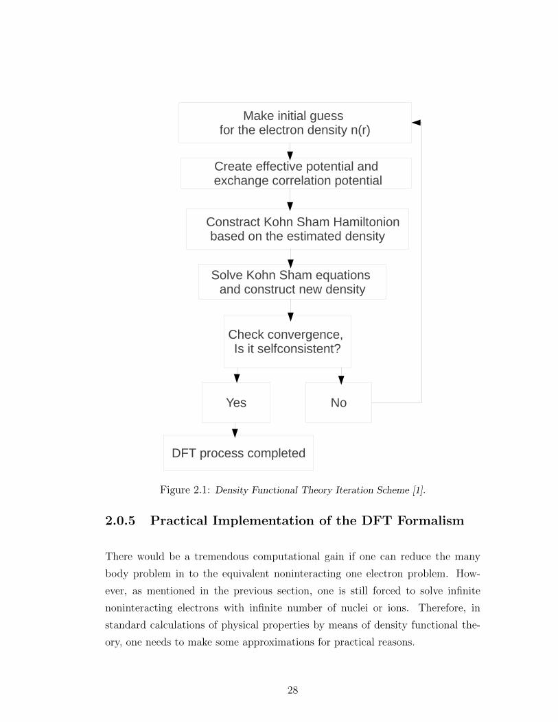
2.0.4.1 DFT Algorithm

In practice, Kohn-Sham equations are solved numerically by an iterative pro-

cedure called self-consistency loop. The process starts with initial guess of the

density and creating effective potential and exchange correlation potentials. By

solving Kohn-Sham equations, a new density is constructed. It is a cyclic step and

in each step, energy is calculated and the process should converge at the ground

state energy. If there is geometry optimization, ionic relaxation takes place in

the end of each steps. Atoms are moved in the end of each cyclic step. When

forces are minimized on the system, the ionic relaxation ends. The diagram of

this process is shown in figure 2.1.

27

��

��

��

��

��!�"�� #

$�� %�

&'(��

Figure 2.1: Density Functional Theory Iteration Scheme [1].

2.0.5 Practical Implementation of the DFT Formalism

There would be a tremendous computational gain if one can reduce the many

body problem in to the equivalent noninteracting one electron problem. How-

ever, as mentioned in the previous section, one is still forced to solve infinite

noninteracting electrons with infinite number of nuclei or ions. Therefore, in

standard calculations of physical properties by means of density functional the-

ory, one needs to make some approximations for practical reasons.

28

2.0.5.1 Crystal Lattice Structure and Bloch Theorem

It is impossible deal with infinite number of electrons in extended system with low

symmetry. For instance in solids, there are infinitely many number of electrons

nuclei and ions. Therefore, it is beneficial to use crystal structure. Since it has the

translational symmetry, periodic boundary conditions makes the process hugely

simplified. A crystal structure is defined by the primitive lattice vectors and the

coordinates of atoms in a primitive unit cell. The primitive lattice vector is given

by

R = n1a1 + n2a2 + n3a3 , (2.10)

where n1, n2, n3 are intergers and a1, a2, a3 are primitive lattice vectors in real

space. In order to describe electronic behavior, one has to work in reciprocal

space (also called momentum space). It is inverse space of the real space. [49]

The reciprocal lattice vector is given by

G = m1b1 +m2b2 +m3b3 , (2.11)

where m1,m2,m3 are intergers and b1, b2, b3 are primitive lattice vectors in

reciprocal space. Any position vector R and reciprocal lattice vector G defines

the reciprocal space;

exp (iGR) = 1 , (2.12)

Translational periodicity of the Brilloin zone allows us to write the potential

as ;

V (r + R) = V (r) , (2.13)

Notice that we write the potential in single particle Hamiltonian. Bloch theorem

states that one can write the wave function in a periodic potential in the form of

a plane waves times a function with the periodicity of the lattice [1].

ψi(r) = exp (ik.R) fi(r) , (2.14)

where fi(r) has the full periodicity of the lattice. One can expand this function

in terms of discrete plane-wave basis set with reciprocal lattice vectors G

fi(r) =∑G

ci,G exp (iG.R) , (2.15)

29

where ci,G are plane wave coefficient. Then we have the wavefunction as

ψi(r) =∑G

ci,k+G exp (i(k + G).R) , (2.16)

Primitive unit cell of the reciprocal space is called Brilloine zone. Usually k points

in the Brilloine zone is sampled such that electronic wavefunctions in k space is

represented by the single k point. [1] There are several important schemes for k

point sampling. Monkhorst-Pack scheme is very useful and widely used method

for k point sampling. This simple formula propesed by Monkhorst and Pack [50]

and defines uniform set of points which is given by

kn1,n2,n3 =∑i

2ni −Ni − 1

2Ni

Gi , (2.17)

where Gi are the primitive lattice vectors of the reciprocal lattice.[51] The choice

of k point depend on the type of crystal structure and it represents uniform grid

of the structure. Further, perhaps even greater this formula defines the periodic

structure which enables electronic structure calculation easier.

2.0.5.2 Plane Waves

Using plane waves as basis set for the electronic structure calculations have several

important aspects. Bloch Theorem is the starting point because this theorem

defines the relation of discrete plane wave basis set. It is not possible to expand

wave function by using infinite number of plane wave basis set. However, one can

reduce this required plane wave basis set by introducing kinetic energy cutoff.

Plane waves with smaller kinetic energy is of utmost importance at that point

because plane waves smaller than some particular cutoff energy is not going to be

taken in to account. It enables easier calculation of energy derivatives and thus

very adequete approach for atomic relaxation and etc. Moreover, it introduces

periodic boundary conditions to the system and it is easy to make calculation

by fourier transformation method. On the other hand, using plane wave basis

set might in some cases cause some errors. Especially, they are not enough to

define the behavior of core electrons therefore, it only gives accurate results for

30

the valence electrons and one needs to use help of pseudopotential method for

the behavior of core states.

2.0.5.3 Pseudopotentials and PAW

It is very difficult to deal with highly localized states such as core electrons due

to strong ionic potential in this region. In the majority of modern electronic

structure calculations the nuclear attraction potentials as well as the atomic core

electrons are pseudized away and replaced by smooth potentials causing slowly

varying densities in the core of the atoms. In this approach, valence states should

be orthogonal to the core states. Thus, the standart electron ion interaction

is replaced by the smooth pseudopotential in the calculations. Pseudoatomic

wavefunctions oscillates slower and that means it requires less number of plane

waves. In principle, core electrons are treated as frozen electrons and they have

no contribution to the chemical bonds. Therefore, the only contribution comes

from valence states. Several important schemes are devised for pseudopotential

approximation. In this thesis, the Projector Augmented wave method [52] is

always followed and it is one the most important way of treating the rapidly

oscillating wavefunction.

2.0.5.4 Van der Waals Interactions

Total potential energy between a pair of neutral atoms or molecules are approx-

imated by Lennard Jones potential which is written as [53]

φ(r) = −4ε

[(σ

r

)6

−(σ

r

)12], (2.18)

where ε is the depth of the potential well, and σ is the distance at which inter-

particle potential is zero and r is the distance between particles. This potential

has two terms, the attractive term which includes van der waals interactions with

r−6 term and the repulsive term which is proportional to r−12. The latter is

associated with the Pauli exclusion principle which states that two fermions can

not be in the same state.

31

Van der Waals interaction, r−6 term on the other hand, arises from the long

range interaction of electrons in the system. Quantum thermal fluctuations will

always induce a dipole even in the neutral atom. The resulting electric field

polarizes the other atom with the order of r−3. The interaction is then in the

order of r−6. This correlation effect is also known as London dispersion and the

resulting are attractive. In electronic structure calculations, this term has often

been neglegted, however, in the scope of physisorption as mentioned above, van

der Waals interactions play an important role. Although it does not care with the

sharing of electrons like in covalent bond or ionic bonds, the long range effects

of electrons are have also considerable effects. Furthermore, in first principle

calculations, it is possible to include C6 term as an extra term to take care of

these long range interactions. As it has been also verified in this thesis, the

contribution of van der Waals interactions can not be neglected.

2.0.6 Computational Details

Our calculations have been performed using Quantum Espresso package. [6]. In

each electronic step Quantum Espresso calculates the forces on the system and

then slightly corrects the initial guess of the density. This procedure continues

with number of electronic step until the total electronic energy is minimized.

This iteration ends until the change in the energy change of each consecutive

selfconsistency step is less than 10−4 Rydberg. When the estimated energy error

is less than 10−6 Rydberg the selfconsistency is achieved.

In order to build the unit cell these hexagonal lattice of carbon structures

and corresponding adsorbates system, XCRYSDEN package [54] is used. The

system is periodic in three dimensions with 20 A along z axis in order to prevent

interactions in this directions. The periodic supercell of 4 × 4 was used with

generalized gradient approximation of Perdew Burke Ernzerhof (PBE) for the

exchange correlation energies. For comparison purposes we have also tested local

density approximations in some particular systems. Quantum espresso input file

overrides the value of exchange correlation type from the pseudopotential part

of the code. In the case of physisorption is studied, exchange correlation part

32

is treated with van der Waals interaction which is implemented in Quantum

Espresso package. Plane wave basis set is used with kinetic energy cutoff of 625

eV. Kinetic energy cutoff for the charge density and potential is usually taken to

be four times higher than the kinetic energy cutoff for the wavefunctions in order

this parameter to be accurately converged. Indeed, testing of this parameters is

mandatory for the accurate results.

33

2.0.6.1 Geometry Optimization and Single Point Energy Calculations

During the geometry optimization, atomic positions are changed until all the

forces on the structure becomes less than the convergence parameter. In this

thesis, structural optimization is performed using Broyden-Fletcher-Goldfarb-

Shanno (BFGS) algorithm. In every iteration, forces and total energy are cal-

culated and atomic positions change in a small distance. We have performed

single point energy calculation in order to test some external parameters, such

as kpoint convergence, energy cutoff convergency. We have investigated inter-

layer distance of graphite structure by performing single point energy runs using

different approximations. It is important to notice the position of minima, if

it exists. The single point energy calculations by local density approximations

results in 3.59 Angstrom interlayer distance whereas van der Waals corrections

gives 3.69 Angstrom. Generalized gradient approximation doesn’t exhibit an en-

ergy barrier, thus minimum value of interlayer distance is difficult to obtain. It

is already known that generalized gradient approximation tends to overestimate

lattice constant although it gives good cohesive energy. In order to investigate

the cohesive energy difference by use of different pseudopotential, single energy

runs have been performed. Different cut-off energies have been tested for all

systems. 500 eV is found to be suitable parameter for both graphite and single

layer graphene system. Although higher cut-off energies give lower energies, it

doesn’t effect the result considerably. The minimum energy lattice constant of

single layer graphene is obtained as 2.4662 A with 1.423 A C-C distance. Further,

k-point convergence test have been performed in order approximations to work

well enough. K-points are set according to the Monkhorst-Pack scheme. K-point

mesh depends on cell size, hence the k-point convergence tests have been per-

formed for each of the different cells individually. In figure 2.7, it is shown that

convergence has been achieved when 225 k-points are used in the calculation.

34

−0.3

−0.2

−0.1

0

0.1

0.2

0.3

0.4

0.5

0.6

2 3 4 5 6 7 8 9

Coh

esiv

e E

nerg

y (e

V)

Interlayer distance (Å)

LDAGGA

VDW−DF

Figure 2.2: Cohesive Energy of AA stacking graphite calculated within Local Den-sity Approximation(red curve) Generalized Gradient Approximation(green curve) andVDW-DF (blue curve)

−0.25

−0.2

−0.15

−0.1

−0.05

0

0.05

0.1

0.15

0.2

0.25

2 3 4 5 6 7 8 9

Coh

esiv

e E

nerg

y (e

V)


GGALDA

VDW−DF

Figure 2.3: Cohesive Energy of AB stacking graphite calculated within PAW Pseu-dopotential (red curve) and Ultrasoft Pseudopotential (green curve) and VDW-DF(blue curve).

35

−0.1

−0.05

0

0.05

0.1

0.15

0.2

0.25

2 3 4 5 6 7 8 9

Coh

esiv

e E

nerg

y (e

V)


PAWUltrasoft

Figure 2.4: Cohesive Energy of AA stacking graphite calculated within PAW Pseu-dopotential (red curve) and Ultrasoft Pseudopotential (green curve) .

−587

−586.5

−586

−585.5

−585

−584.5

−584

−583.5

−583

200 250 300 350 400 450 500 550 600 650

To

tal E

nerg

y (

eV

)

Ecut (eV)

Energy Cutoff Parameter

Figure 2.5: Cutoff energy convergence graph of AA stacking graphite.

36

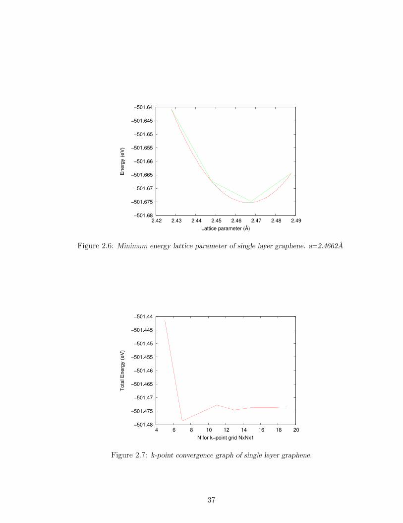
−501.68

−501.675

−501.67

−501.665

−501.66

−501.655

−501.65

−501.645

−501.64

2.42 2.43 2.44 2.45 2.46 2.47 2.48 2.49

Ene

rgy

(eV

)

Lattice parameter (Å)

Figure 2.6: Minimum energy lattice parameter of single layer graphene. a=2.4662A

−501.48

−501.475

−501.47

−501.465

−501.46

−501.455

−501.45

−501.445

−501.44

4 6 8 10 12 14 16 18 20

To

tal E

ne

rgy (

eV

)

N for k−point grid NxNx1

Figure 2.7: k-point convergence graph of single layer graphene.

37

Chapter 3

Results and Discussion

Several researchers have investigated several important schemes to find stable

configurations of hydrogen or halogen atoms adsorbed on graphene and have re-

ported important properties of these systems such as charge transfer between

adatom and graphene, work function difference in the energy band diagram. The

main goal of these works is to change hybridization from sp2 to sp3. When the

adatom is adsorbed on graphene, the additional electron is localized on pz like

orbital thus is a suitable candidate to form covalent bond along z direction. This

results in opening a band gap, which would be enormous distribution for elec-

tronic devices. For this purpose, a variety of systems and approximations are

investigated which will be useful to understand electronic and structural prop-

erties of functionalized graphene. Stability of these systems are investigated by

comparing binding energy values.

3.1 Calculation of Binding Energy

Binding energies are calculated using

EB = Ead−gra − Egra − nEad , (3.1)

38

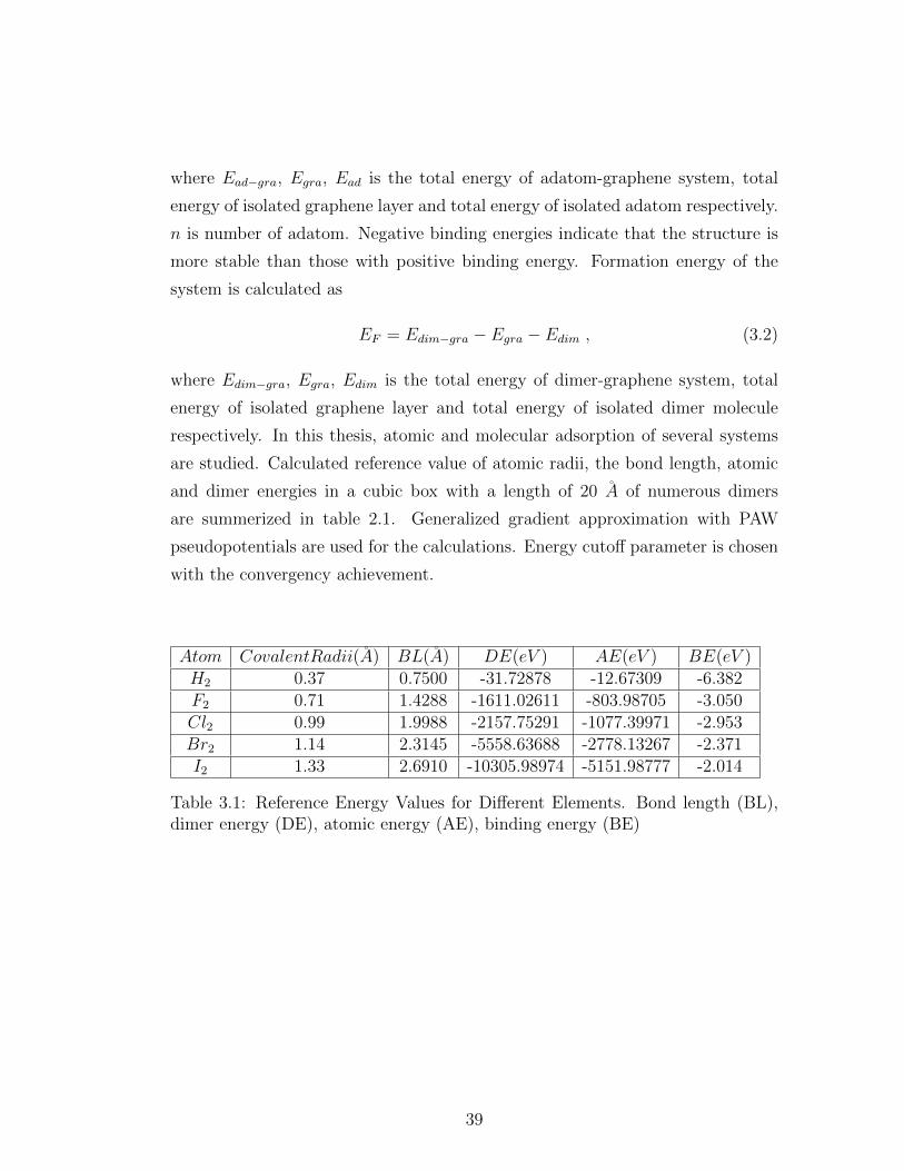
where Ead−gra, Egra, Ead is the total energy of adatom-graphene system, total

energy of isolated graphene layer and total energy of isolated adatom respectively.

n is number of adatom. Negative binding energies indicate that the structure is

more stable than those with positive binding energy. Formation energy of the

system is calculated as

EF = Edim−gra − Egra − Edim , (3.2)

where Edim−gra, Egra, Edim is the total energy of dimer-graphene system, total

energy of isolated graphene layer and total energy of isolated dimer molecule

respectively. In this thesis, atomic and molecular adsorption of several systems

are studied. Calculated reference value of atomic radii, the bond length, atomic

and dimer energies in a cubic box with a length of 20 A of numerous dimers

are summerized in table 2.1. Generalized gradient approximation with PAW

pseudopotentials are used for the calculations. Energy cutoff parameter is chosen

with the convergency achievement.

Atom CovalentRadii(A) BL(A) DE(eV ) AE(eV ) BE(eV )H2 0.37 0.7500 -31.72878 -12.67309 -6.382F2 0.71 1.4288 -1611.02611 -803.98705 -3.050Cl2 0.99 1.9988 -2157.75291 -1077.39971 -2.953Br2 1.14 2.3145 -5558.63688 -2778.13267 -2.371I2 1.33 2.6910 -10305.98974 -5151.98777 -2.014

Table 3.1: Reference Energy Values for Different Elements. Bond length (BL),dimer energy (DE), atomic energy (AE), binding energy (BE)

39

Figure 3.1: Single sided hydrogenated graphene.

Figure 3.2: Dimer hydrogen adsorbed graphene.

40

Figure 3.3: Chair configuration hydrogenated graphene.

3.2 Hydrogen Adsorption

We begin with hydrogenated graphene called ”graphane” [29] which is to our

knowledge one among the very first studied adsorbate on single layer graphene for

band gap engineering through chemical modification. Hydrocarbons are simplest

commonly found organic componds of nature. Sofo et al., found that graphane

is two dimensional covalently bonded hydrocarbon. There are numerous studies

on graphane, hence, the results reported here can be compared with the previous

works. Attachment of the hydrogen atoms leads each carbon atoms of graphene

to make an additional bond giving rise to change in hybridization by crumpling

the structure. Starting with fully covered single sided hydrogenated graphene

structure, different configurations of graphane have been studied. The relaxation

process have been performed and minimum energy lattice constant has been ob-

tained. The unit cell of the graphene sheet is 4 × 4 since it is not possible to

perform all configurations in a smaller unit cell. Energy cutoff parameter is set

to 625 eV. Results are summarized in table 3.1.

The results show that the lattice parameter is longer than the lattice pa-

rameter of single layer graphene. The behavior for smaller lattice constant is

41

Figure 3.4: Boat configuration hydrogenated graphene.

Configuration a Ch dC−C dC−H dH−H θC−C−H BE/bond Eg

Single sided 2.83 0.020 1.637 1.074 1.636 90.20 -1.570 1.257Dimer adsorbed 2.49 0.000 1.413 3.351 0.730 90.00 -5.985 -

Chair 2.54 0.463 1.537 1.109 2.520 107.03 -3.286 3.352Boat 2.50 0.647 1.531 1.104 2.202 107.09 -3.181 3.233

Zigzag 2.44 1.035 1.585 1.106 2.242 105.11 -3.108 2.784Armchair 2.42 1.090 1.551 1.102 2.179 106.28 -3.102

Table 3.2: Calculated structural properties and binding energy of different config-urations of graphane: lattice constant (a)(A), buckling (Ch) (A), distance betweenC atoms, H-C atoms and H atoms are (dC−C),(dC−H), (dH−H) (A) respectively.Angle between carbon and hydrogen atoms (θC−C−H), binding energy per bond(BE)(eV), Energy gap (Eg) (eV), formation energy of dimer adsorbed: 0.375 eV.

different. Strong covalent character of carbon-carbon bond makes correspond-

ing carbon-hydrogen interactions weaker. Furthermore, since hydrogen atoms

becomes closer, they form dimer molecule and escape. This result has led us

to study hydrogen dimer molecules on top of graphene layer. Indeed, van der

Waals interaction plays important role for the present interaction, therefore, we

used vdW functional for the exchange correlation part of the total energy as op-

posed to the previous case that has been performed with generalized gradient ap-

proximation. It seems dimer molecule adsorption on graphene gives more stable

structure when compared to the binding energy of previous calculation. How-

ever, formation energy of this structure is 0.375 eV which indicates instability.

42

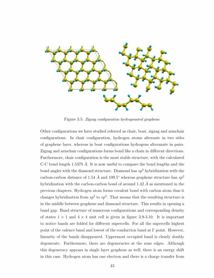
Figure 3.5: Zigzag configuration hydrogenated graphene.

Other configurations we have studied referred as chair, boat, zigzag and armchair

configurations. In chair configuration, hydrogen atoms alternate in two sides

of graphene layer, whereas in boat configurations hydrogens alteranate in pairs.

Zigzag and armchair configurations forms bond like a chain in different directions.

Furthermore, chair configuration is the most stable structure, with the calculated

C-C bond length 1.5379 A. It is now useful to compare the bond lengths and the

bond angles with the diamond structure. Diamond has sp3 hybridization with the

carbon-carbon distance of 1.54 A and 109.5◦ whereas graphene structure has sp2

hybridization with the carbon-carbon bond of around 1.42 A as mentioned in the

previous chapters. Hydrogen atom forms covalent bond with carbon atom thus it

changes hybridization from sp2 to sp3. That means that the resulting structure is

in the middle between graphene and diamond structure. This results in opening a

band gap. Band structure of numerous configurations and corresponding density

of states 1 × 1 and 4 × 4 unit cell is given in figure 3.9-3.10. It is important

to notice bands are folded for different supercells. For all the supercells highest

point of the valence band and lowest of the conduction band at Γ point. However,

linearity of the bands disappeared. Uppermost occupied band is clearly doubly

degenerate. Furthermore, there are degeneracies at the zone edges. Although

this degeneracy appears in single layer graphene as well, there is an energy shift

in this case. Hydrogen atom has one electron and there is a charge transfer from

43

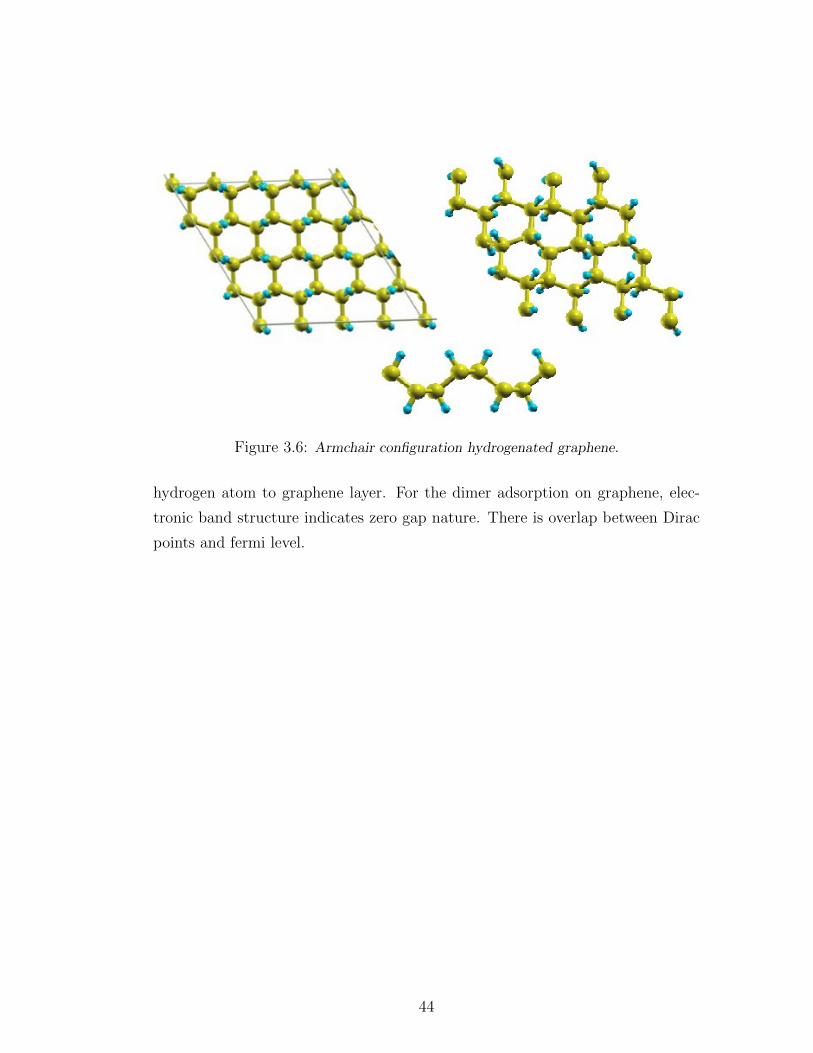
Figure 3.6: Armchair configuration hydrogenated graphene.

hydrogen atom to graphene layer. For the dimer adsorption on graphene, elec-

tronic band structure indicates zero gap nature. There is overlap between Dirac

points and fermi level.

44

−20

−15

−10

−5

0

5

En

erg

y (

eV

)

Γ K M K 1 2 3 4

DOS(electron/eV)

H−pdos

Figure 3.7: Band structure and density of states of singleside configuration hydro-genated graphene of 1× 1 unit cell.

−20

−15

−10

−5

0

5

Energ

y (

eV

)

Γ K M KDOS(electron/eV)

Figure 3.8: Band structure and density of states of dimer adsorbed hydrogenatedgraphene of 1× 1 unit cell.

45

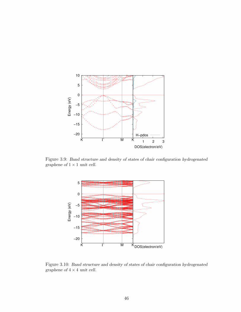
−20

−15

−10

−5

0

5

10

En

erg

y (

eV

)

Γ K M K 1 2 3

DOS(electron/eV)

H−pdos

Figure 3.9: Band structure and density of states of chair configuration hydrogenatedgraphene of 1× 1 unit cell.

−20

−15

−10

−5

0

5

Energ

y (

eV

)


Figure 3.10: Band structure and density of states of chair configuration hydrogenatedgraphene of 4× 4 unit cell.

46

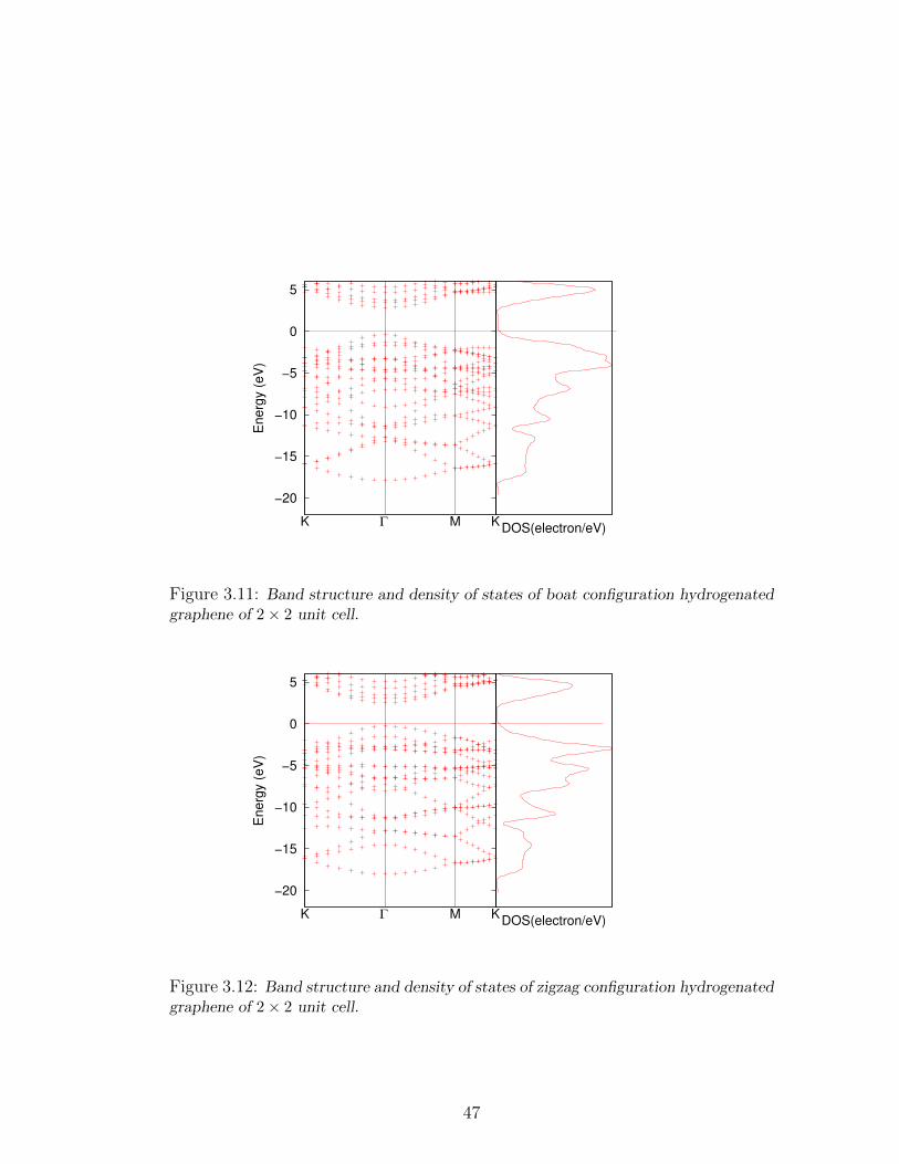
−20

−15

−10

−5

0

5

En

erg

y (

eV

)


Figure 3.11: Band structure and density of states of boat configuration hydrogenatedgraphene of 2× 2 unit cell.

−20

−15

−10

−5

0

5

Energ

y (

eV

)


Figure 3.12: Band structure and density of states of zigzag configuration hydrogenatedgraphene of 2× 2 unit cell.

47

Figure 3.13: Single F adsoption on top of the carbon atom on graphene.

Figure 3.14: Single F adsoption in the middle of carbon-carbon bond on graphene.

48

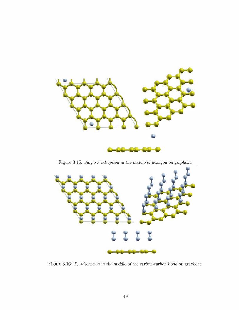
Figure 3.15: Single F adsoption in the middle of hexagon on graphene.

Figure 3.16: F2 adsorption in the middle of the carbon-carbon bond on graphene.

49

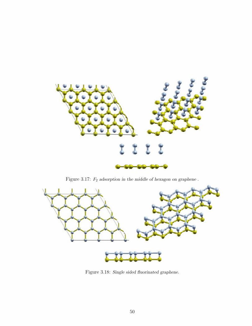
Figure 3.17: F2 adsorption in the middle of hexagon on graphene .

Figure 3.18: Single sided fluorinated graphene.

50

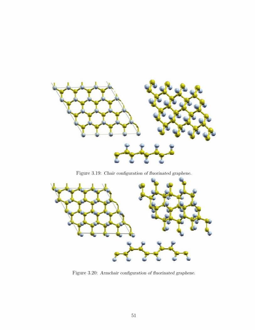
Figure 3.19: Chair configuration of fluorinated graphene.

Figure 3.20: Armchair configuration of fluorinated graphene.

51

Figure 3.21: Boat configuration of fluorinated graphene.

Figure 3.22: Zigzag configuration of fluorinated graphene.

52

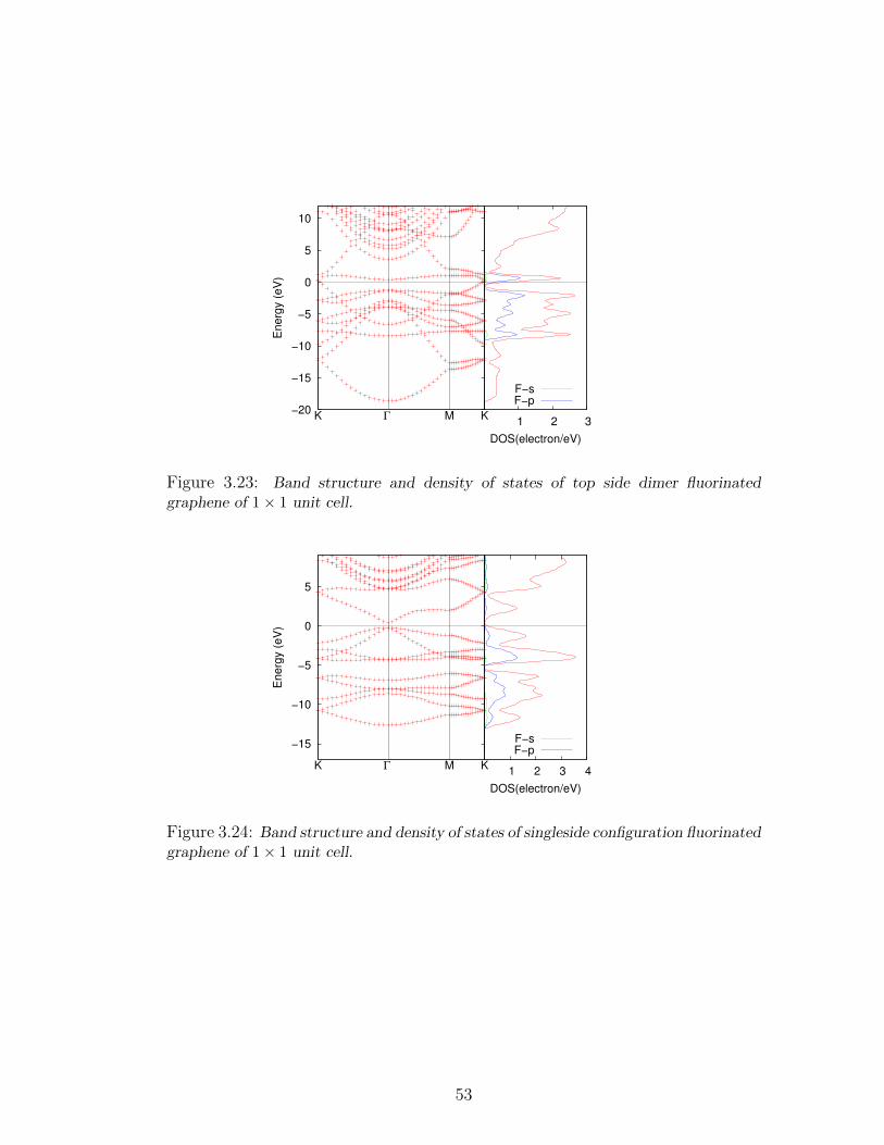
−20

−15

−10

−5

0

5

10

Energ

y (

eV

)

Γ K M K 1 2 3

DOS(electron/eV)

F−sF−p

Figure 3.23: Band structure and density of states of top side dimer fluorinatedgraphene of 1× 1 unit cell.

−15

−10

−5

0

5

Energ

y (

eV

)

Γ K M K 1 2 3 4

DOS(electron/eV)

F−sF−p

Figure 3.24: Band structure and density of states of singleside configuration fluorinatedgraphene of 1× 1 unit cell.

53

−15

−10

−5

0

5

10

Energ

y (

eV

)

Γ K M K 1 2 3 4

DOS(electron/eV)

F−sF−p

Figure 3.25: Band structure and density of states of singleside dimer fluorinatedgraphene of 1× 1 unit cell.

−15

−10

−5

0

5

10

Energ

y (

eV

)

Γ K M K 1 2 3 4

DOS(electron/eV)

F−sF−p

Figure 3.26: Band structure and density of states of chair configuration fluorinatedgraphene of 1× 1 unit cell.

54

−15

−10

−5

0

5

Energ

y (

eV

)

Γ K M K 2 4 6 8 10

DOS(electron/eV)

F−sF−p

Figure 3.27: Band structure and density of states of boat configuration fluorinatedgraphene of 2× 2 unit cell.

−20

−15

−10

−5

0

5

10

Energ

y (

eV

)

Γ K M K 2 4 6 8 10

DOS(electron/eV)

F−sF−p

Figure 3.28: Band structure and density of states of zigzag configuration fluorinatedgraphene of 2× 2 unit cell.

55

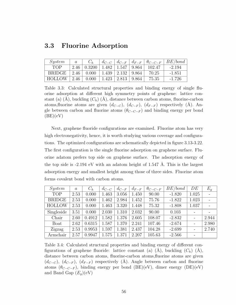
3.3 Fluorine Adsorption

System a Ch dC−C dC−F dF−F θC−C−F BE/bondTOP 2.46 0.3200 1.482 1.547 9.864 102.47 -2.194

BRIDGE 2.46 0.000 1.439 2.132 9.864 70.25 -1.851HOLLOW 2.46 0.000 1.423 2.813 9.864 75.35 -1.726

Table 3.3: Calculated structural properties and binding energy of single flu-orine adsorption at different high symmetry points of graphene: lattice con-stant (a) (A), buckling (Ch) (A), distance between carbon atoms, fluorine-carbonatoms,fluorine atoms are given (dC−C), (dC−F ), (dF−F ) respectively (A). An-gle between carbon and fluorine atoms (θC−C−F ) and binding energy per bond(BE)(eV)

Next, graphene fluoride configurations are examined. Fluorine atom has very

high electronegativity, hence, it is worth studying various coverage and configura-

tions. The optimized configurations are schematically depicted in figure 3.13-3.22.

The first configuration is the single fluorine adsorption on graphene surface. Flu-

orine adatom prefers top side on graphene surface. The adsorption energy of

the top side is -2.194 eV with an adatom height of 1.547 A. This is the largest

adsorption energy and smallest height among those of three sides. Fluorine atom

forms covalent bond with carbon atoms.

System a Ch dC−C dC−F dF−F θC−C−F BE/bond DE EgTOP 2.53 0.000 1.463 3.056 1.450 90.00 -1.820 1.025 -

BRIDGE 2.53 0.000 1.462 2.984 1.452 75.76 -1.822 1.023 -HOLLOW 2.53 0.000 1.463 3.320 1.448 75.32 -1.808 1.037 -

Singleside 3.51 0.000 2.030 1.310 2.032 90.00 0.103 - -Chair 2.60 0.4912 1.582 1.376 2.605 108.07 -2.832 - 2.944Boat 2.62 0.6315 1.587 1.370 2.241 107.46 -2.674 - 2.980

Zigzag 2.53 0.9953 1.597 1.381 2.437 104.28 -2.699 - 2.740Armchair 2.57 0.9947 1.575 1.371 2.207 105.63 -2.566 -

Table 3.4: Calculated structural properties and binding energy of different con-figurations of graphene fluoride: lattice constant (a) (A), buckling (Ch) (A),distance between carbon atoms, fluorine-carbon atoms,fluorine atoms are given(dC−C), (dC−F ), (dF−F ) respectively (A). Angle between carbon and fluorineatoms (θC−C−F ), binding energy per bond (BE)(eV), dimer energy (DE)(eV)and Band Gap (Eg)(eV)

56

Then, dimer molecules adsorption on graphene have been studied. The opti-

mal adsorption positions on graphene surface are determined and binding energies

are calculated. The results show that adsorption energy and adatom heights are

very similar to each other for different adsorption sides. Still, bridge side is more

favorable with 2 meV difference. Furthermore, final F-F bond distance is around

1.45 A. The resulting C-F distance shows that there is a van der Waals interaction

present between fluorine dimer and carbon atoms. Also, full coverage of fluorine

atoms on graphene are considered. The structure called fluorographene in which

carbon atoms alternates on top and bottom sides of the graphene layer is the most

stable structure. Indeed, graphene planar surface are buckled and carbon-carbon

bond length increased. The angle between graphene surface and adsorbed atom

is around 109◦. Hence, it is obvious that fluorographene is sp3 like rehybridized.

Moreover, the binding energy of boat configuration slightly less than chair con-

figuration which is due to F-F repulsion. Finally, zigzag configuration is found to

be more stable than armchair configuration.

57

3.4 Chlorine Adsorption

System a Ch dC−C dC−Cl dCl−Cl θC−C−Cl BE/bondTOP 2.46 0.000 1.423 3.234 9.864 89.79 -1.103

BRIDGE 2.46 0.000 1.424 3.294 9.864 77.52 -1.101HOLLOW 2.46 0.000 1.423 3.535 9.864 78.39 -1.102

Table 3.5: Calculated structural properties and binding energy of single chlo-rine adsorption at different high symmetry points of graphene: lattice constant(a) (A), buckling (Ch) (A), distance between carbon atoms, chlorine-carbonatoms,chlorine atoms are given (dC−C), (dC−Cl), (dCl−Cl) respectively (A). An-gle between carbon and fluorine atoms (θC−C−Cl) and binding energy per bond(BE)(eV)

Third system is chlorinated graphene. Again, three different positions of single

and dimer chlorine atoms has been considered i.e top, bridge and hollow. Binding

energies at different sides appears to be rather similar. This is due to relatively

large radius of chlorine atom compared to fluorine. It has very large lattice

constant for single side adsorption. For smaller lattice constant, the stronger

carbon-carbon bond makes corresponding carbon-chlorine bond weaker, hence

chlorine atoms form layer structure. The dimer adsorption doesn’t give different

binding energies at different positions. However, it forms chlorine layers with the

distance 3.9 A between them. Only the top side adsorption is presented in table

3.6. For the full coverage of chlorine, the chair configuration exhibits different

behavior than chair configuration of fluorinated graphene.

System a Ch dC−C dC−Cl dCl−Cl θC−C−Cl BE/bond DE EgTOP 2.59 0.000 1.499 4.112 3.970 90.19 -0.632 1.587 -

Singleside 5.19 0.000 2.995 1.651 3.000 90.03 2.827 - -NB Chair 2.60 0.000 1.501 3.722 2.594 90.00 -0.472 - -

Chair 2.91 0.5079 1.755 1.750 2.910 106.79 -0.030 - 1.908Boat 3.02 0.6242 1.748 1.718 2.577 106.97 0.365 - 0.930

Table 3.6: Calculated structural properties and binding energy of different con-figurations of chlorinated graphene : lattice constant (a) (A), buckling (Ch) (A),distance between carbon atoms, chlorine-carbon atoms,chlorine atoms are given(dC−C), (dC−Cl), (dCl−Cl) respectively (A). Angle between carbon and fluorineatoms (θC−C−Cl) and binding energy per bond (BE)(eV), Band Gap (Eg) (eV)

There are two stable configurations in chair structure, referred as, nonbonded

58

and bonded. For smaller lattice constant, chlorine atoms exhibit nonbonded sta-

ble configurations. The repulsion between nonbonded atoms and carbon atoms

are compansated with van der Waals forces, as a result, atoms reach their equi-

librium position. In the bonded system on the other hand, there is a strong

covalent character, because carbon-chlorine bond is stronger. Boat configuration

gives positive binding energy value, therefore it is not stable configuration. Zigzag

and armchair initial configurations forms completely different lattice, therefore

graphene layer doesn’t remain in its original honeycomb shape. Band structure

calculations show that chlorine adsorption results in energy gap for chair and

boat conformations.

59

Figure 3.29: Single chlorine adsorption on top of carbon atom on graphene.

Figure 3.30: Single chlorine adsorption in the middle of carbon-carbon bond ongraphene.

Figure 3.31: Single chlorine adsorption in the middle of hexagon on graphene.

60

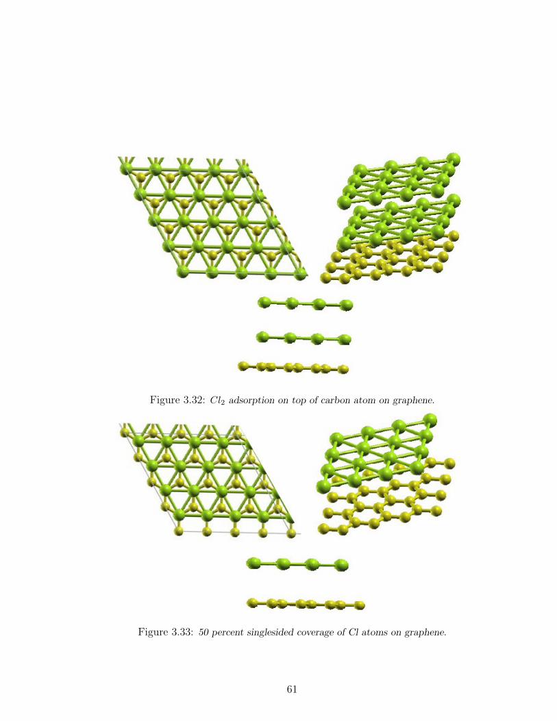
Figure 3.32: Cl2 adsorption on top of carbon atom on graphene.

Figure 3.33: 50 percent singlesided coverage of Cl atoms on graphene.

61

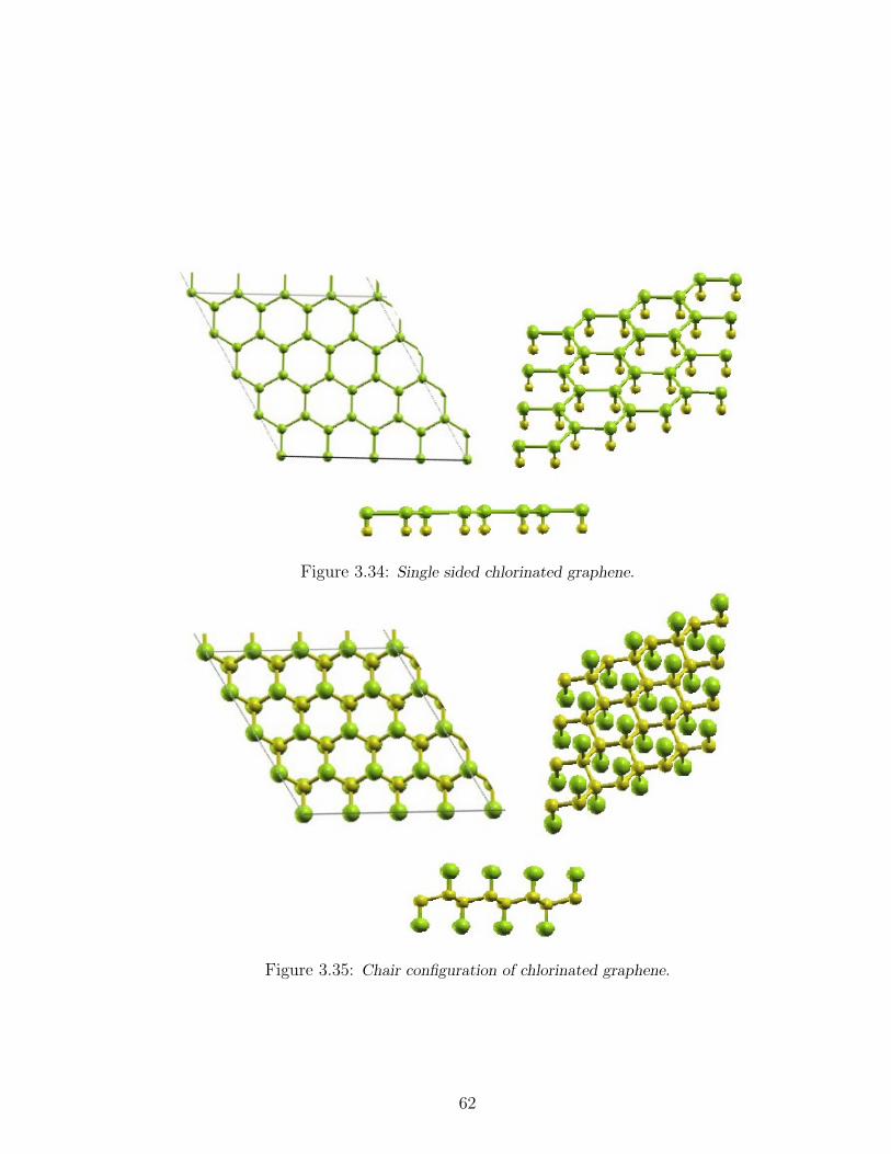
Figure 3.34: Single sided chlorinated graphene.

Figure 3.35: Chair configuration of chlorinated graphene.

62

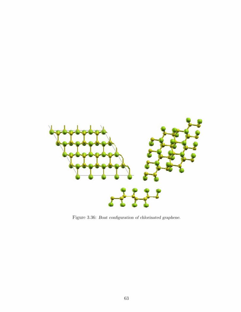
Figure 3.36: Boat configuration of chlorinated graphene.

63

−20

−15

−10

−5

0

5

En

erg

y (

eV

)

Γ K M K 2 4 6 8

DOS(electron/eV)

Cl−sCl−p

Figure 3.37: Band structure and density of states of singleside configuration chlori-nated graphene of 1× 1 unit cell.

−20

−15

−10

−5

0

5

Ene

rgy (

eV

)

Γ K M K 2 4 6 8

DOS(electron/eV)

Cl−sCl−p

Figure 3.38: Band structure and density of states of chair configuration chlorinatedgraphene of 1× 1 unit cell.

64

−20

−15

−10

−5

0

5

10

En

erg

y (

eV

)

Γ K M K 2 4

DOS(electron/eV)

Cl−sCl−p

Figure 3.39: Band structure and density of states of nonbonded chair configurationchlorinated graphene of 1× 1 unit cell.

−20

−15

−10

−5

0

5

Ene

rgy (

eV

)

Γ K M K 2 4 6 8 10

DOS(electron/eV)

Cl−sCl−p

Figure 3.40: Band structure and density of states of boat configuration chlorinatedgraphene of 2× 2 unit cell.

65

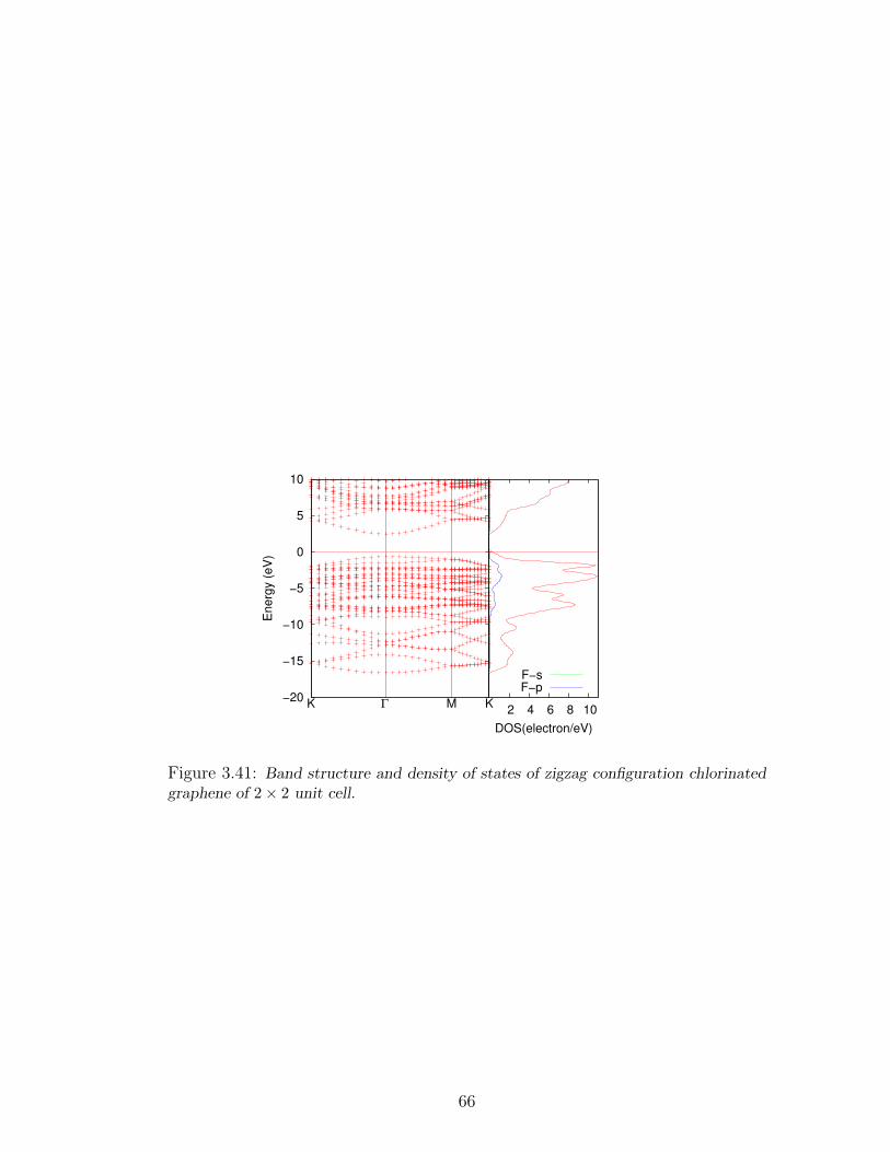
−20

−15

−10

−5

0

5

10

En

erg

y (

eV

)

Γ K M K 2 4 6 8 10

DOS(electron/eV)

F−sF−p

Figure 3.41: Band structure and density of states of zigzag configuration chlorinatedgraphene of 2× 2 unit cell.

66

3.5 Bromide Adsorption

System a Ch dC−C dC−Br dBr−Br BE/bondTOP 2.46 0.00 1.423 3.445 9.84 -0.871

BRIDGE 2.46 0.00 1.424 3.509 9.84 -0.871HOLLOW 2.46 0.00 1.423 3.731 9.84 -0.871

Table 3.7: Calculated structural properties and binding energy of single bromideadsorption at different high symmetry points of graphene: different configura-tions of bromide-graphene: lattice constant (a) (A), buckling (Ch) (A), distancebetween carbon atoms, bromide-carbon atoms, bromide atoms are given (dC−C),(dC−Br), (dBr−Br) respectively (A). and binding energy per bond (BE)(eV)

System a Ch dC−C dC−Br dBr−Br θC−C−Br BE/bond DE EgTOP 2.72 0.0000 1.574 3.864 4.071 90.0 0.219 2.435 -

Singleside 5.75 0.0000 3.319 1.827 3.320 90.0 3.743 - -NB Chair 2.72 0.0000 1.570 3.906 2.7207 90.0 0.225 - -

Chair 3.10 0.4961 1.861 1.924 3.108 105.4 1.364 - -Boat 3.24 0.5645 1.828 1.907 2.776 104.6 1.741 - -

Table 3.8: Calculated structural properties and binding energy of different con-figurations of bromide-graphene: lattice constant (a) (A), buckling (Ch) (A),distance between carbon atoms, bromide-carbon atoms, bromide atoms are given(dC−C), (dC−Br), (dBr−Br) respectively (A). Angle between carbon and bromideatoms (θC−C−Cl), binding energy per bond (BE)(eV), dimer energy (DE) (eV),Band Gap (Eg) (eV)

The same configurations have been tested for bromide adsorption. Single bro-

mide adsorption on graphene doesn’t exhibit any difference in binding energies.

For the full coverage of bromide the results of 4×4 unit cell are presented in table

3.8. For the full coverage of dimer bromide molecules, there is no difference in the

binding energy at different high symmetry sides. After the structures are fully

relaxed, the second atom on dimer molecule escapes and bromide atoms form

layer structure. Bromide adsorption also exhibits non-bonded chair configuration

like in the case of chlorographene. Again, chair configuration is the most favor-

able structure compared to the other configurations. However, bromide graphene

does not exhibit stability. Indeed, it has higher radius and this shows that the

expected final carbon-adsorbate bond length to be higher. Zigzag and armchair

configurations of bromide atoms deformed the graphene structure, thus resulted

67

in different structure. Moreover, there is no gap in the band structure in figures

3.37-3.41.

68

Figure 3.42: Br2 adsorption on top of carbon atom on graphene.

Figure 3.43: Half coverage singlesided coverage of Br atoms on graphene.

69

Figure 3.44: Single sided bromide graphene.

Figure 3.45: Nonbonded chair configuration of bromide graphene.

70

Figure 3.46: Chair configuration of bromide graphene.

Figure 3.47: Boat configuration of bromide graphene.

71

−20

−15

−10

−5

0

5

En

erg

y (

eV

)

Γ K M K 2 4

DOS(electron/eV)

Br−sBr−p

Figure 3.48: Band structure and density of states of singleside monolayer half coveragebromide graphene of 1× 1 unit cell.

−20

−15

−10

−5

0

5

Ene

rgy (

eV

)

Γ K M K 2 4 6 8

DOS(electron/eV)

Br−sBr−p

Figure 3.49: Band structure and density of states of singleside configuration bromidegraphene of 1× 1 unit cell.

72

−15

−10

−5

0

5

10E

ne

rgy (

eV

)

Γ K M K 2 4 6 8

DOS(electron/eV)

Br−sBr−p

Figure 3.50: Band structure and density of states of nonbonded chair configurationbromide graphene of 1× 1 unit cell.

−20

−15

−10

−5

0

5

Energ

y (

eV

)

Γ K M K 2 4 6 8

DOS(electron/eV)

Br−sBr−p

Figure 3.51: Band structure and density of states of chair configuration bromidegraphene of 1× 1 unit cell.

73

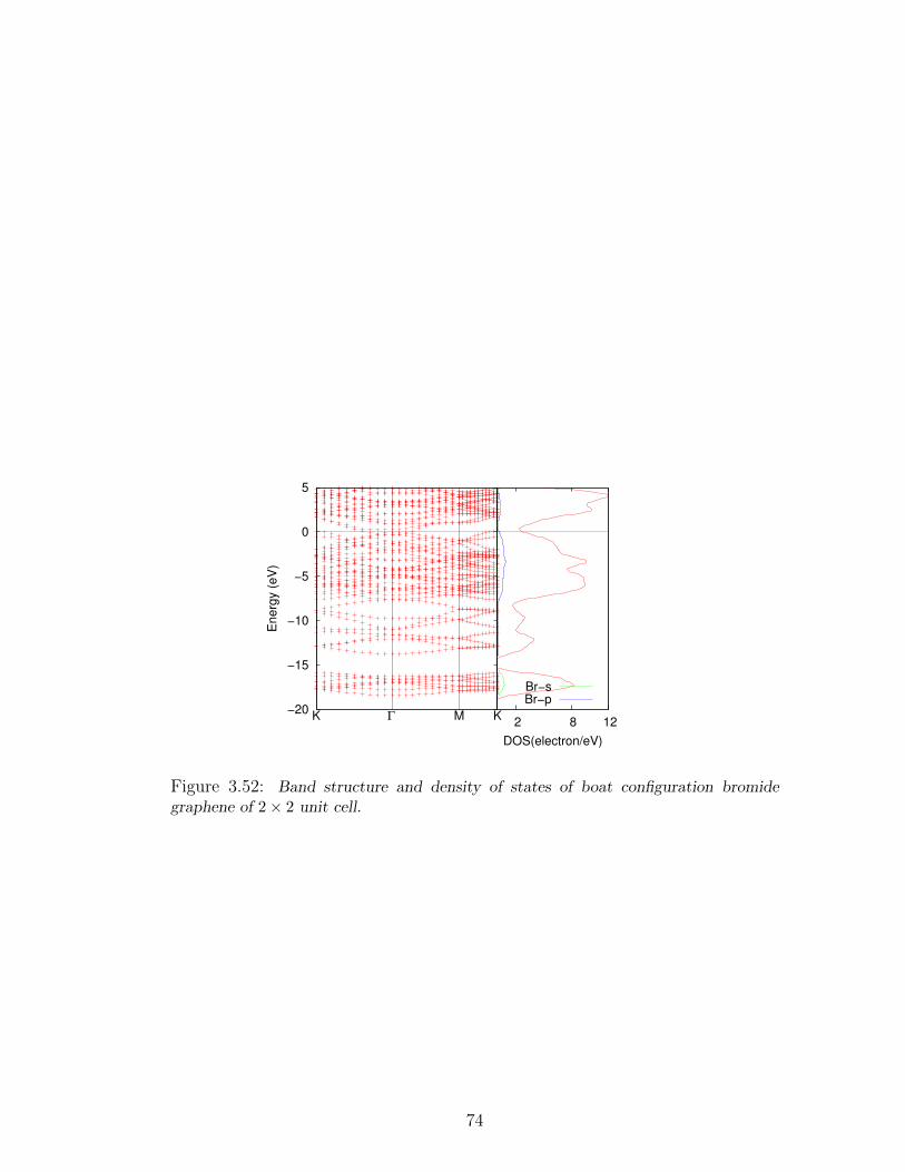
−20

−15

−10

−5

0

5

En

erg

y (

eV

)

Γ K M K 2 8 12

DOS(electron/eV)

Br−sBr−p

Figure 3.52: Band structure and density of states of boat configuration bromidegraphene of 2× 2 unit cell.

74

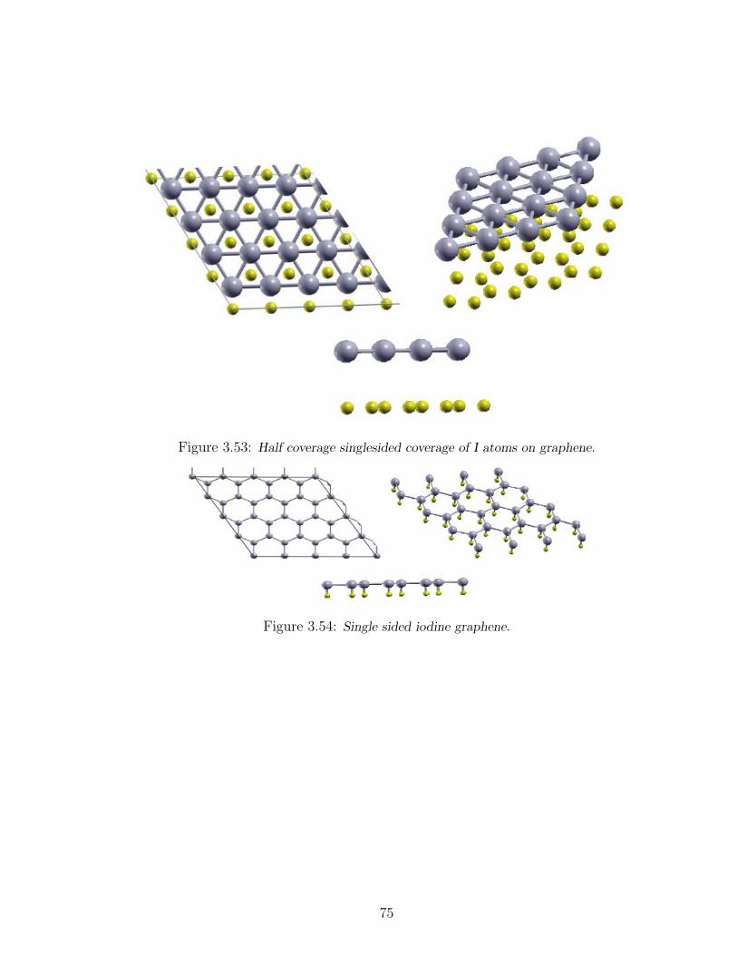
Figure 3.53: Half coverage singlesided coverage of I atoms on graphene.

Figure 3.54: Single sided iodine graphene.

75

Figure 3.55: Nonbonded chair configuration of iodine graphene.

Figure 3.56: Chair configuration of iodine graphene.

76

−20

−15

−10

−5

0

5

En

erg

y (

eV

)

Γ K M K 2 4 6 8

DOS(electron/eV)

I−sI−p

Figure 3.57: Band structure and density of states of singleside monolayer half coverageiodine graphene of 1× 1 unit cell.

−15

−10

−5

0

5

Ene

rgy (

eV

)

Γ K M K 2 4 6 8

DOS(electron/eV)

I−sI−p

Figure 3.58: Band structure and density of states of singleside configuration iodinegraphene of 1× 1 unit cell.

77

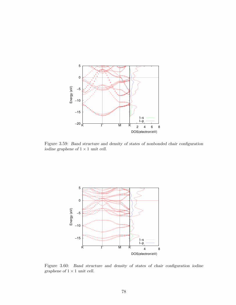
−20

−15

−10

−5

0

5

En

erg

y (

eV

)

Γ K M K 2 4 6 8

DOS(electron/eV)

I−sI−p

Figure 3.59: Band structure and density of states of nonbonded chair configurationiodine graphene of 1× 1 unit cell.

−15

−10

−5

0

5

Energ

y (

eV

)

Γ K M K 4 8

DOS(electron/eV)

I−sI−p

Figure 3.60: Band structure and density of states of chair configuration iodinegraphene of 1× 1 unit cell.

78

3.6 Iodine Adsorption

System a Ch dC−C dC−I dI−I BE/bondTOP 2.46 0.000 1.423 3.717 9.84 -0.669

BRIDGE 2.46 0.000 1.424 3.786 9.84 -0.670HOLLOW 2.46 0.000 1.423 3.968 9.84 -0.670

Table 3.9: Calculated structural properties and binding energy of single iodineadsorption at different high symmetry points of graphene: different configurationsof iodine-graphene: lattice constant (a) (A), buckling (Ch) (A), distance betweencarbon atoms, iodine-carbon atoms, iodine atoms are given (dC−C), (dC−Br),(dBr−Br) respectively (A). Angle between carbon and iodine atoms (θC−C−I) andbinding energy per bond (BE)(eV)

System a Ch dC−C dC−I dI−I θC−C−I BE/bond EgSingleside 6.40 0.000 3.700 2.030 3.7014 - 4.445 -NB Chair 2.96 0.000 1.707 4.000 2.960 - 1.594 -

Chair 3.39 0.4294 1.998 2.61 3.392 102.47 2.623 -

Table 3.10: Calculated structural properties and binding energy of different con-figurations of iodine-graphene: lattice constant (a) (A), buckling (Ch) (A), dis-tance between carbon atoms, iodine-carbon atoms, iodine atoms are given (dC−C),(dC−I), (dI−I) respectively (A). Angle between carbon and iodine atoms (θC−C−I),binding energy per bond (BE)(eV), dimer energy (DE) (eV), Band Gap (Eg) (eV)

Iodine is the largest atom in halogen columns, thus larger initial bond length

was set in order to be able to perform relaxation. As in the previous cases, sin-

gle atom adsorption results in stable structure with -0.67 eV. However, binding

energy does not differ at different high symmetry sides. Full iodine coverage in

chair configuration results in a very large lattice constant. Furthermore, boat,

zigzag and armchair configurations of iodine atoms deformed graphene’s honey-

comb structure. Possible configurations of iodine adsoption can be seen in figures

3.53-3.56. Moreover, iodine dimer adsorption gives 2.748 eV bonding energy.

Overall, this structure is not stable and corresponding band structures show that

there is no energy gap in these structures.

79

Chapter 4

Conclusions

The functionalization of graphene by hydrogen or halogen atoms has been inves-

tigated by plane-wave pseudo-potential calculations based on density functional

theory. It has been investigated that the structures of full coverage of fluorinated

graphene and hydrogenated graphene have similar structures. The fourth valence

electrons of carbon atoms participate covalent bonds. π bands are removed in

the electronic band structure of adsorbed graphene system leading to opening

a band gap. In these adsorbed systems every carbon atom forms 4 bonds thus,

they change the sp2 graphene structure to sp3 by increasing the bond lengths and

decresing bond angles of graphene structure. Fluorine is the lightest atom among

halogen atoms. Stability decreases as the radius of atoms increase and weakening

in electronegativity. Heavier compounds like chlorine, bromide and iodine atoms

exhibit ionic bonding and they do not exhibit very high and strong binding. It

is also clear from the adatom heights in these structures, i.e. 3-4 A which shows

that binding is not covalent type. For the single adatom adsorption only the

fluorine atom is chemically adsorbed on graphene. Chlorine single adatom on

the other hand, exhibits physisorption which shows that chlorine and graphene

interacts weakly. Dimer molecules are found to be relaxed around 3.3 A which

suggests that no bond formation between dimers and carbon atoms of graphene.

Therefore, graphene keeps its original planar structure. For the full coverage,

chair configuration is the most stable structure for all of the systems. Moreover,

80

boat configuration is the second highest among the most stable structure. Smaller

binding energy results from repulsion of the smaller F-F distance positioned on

the same side. For armchair and zigzag configurations there is a considerable

alteration in the planar structure of graphene. The resulting bromide-graphene

and iodine-graphene system exhibits positive binding energy, consequently it is

difficult to use these systems in electronic application, large amount of energy is

required in order to obtain efficient materials. Overall, halogen atoms are useful

for technological applications, adsorption of these atoms in various configura-

tions tailor electronic structure of graphene. Therefore, these systems are very

promising candidates for the future technologies.

81

Bibliography

[1] M. C. Payne, M. P. Teter, D. C. Allan, T. A. Arias, and J. D. Joannopoulos,

“Iterative minimization techniques for ab initio total-energy calculations:

molecular dynamics and conjugate gradients,” Rev. Mod. Phys, vol. 64, 1992.

[2] A. Lavoisier, “Trait lmentaire de chimie,” 1789.

[3] B. T. Kelly, “Physics of graphite,” Applied Science, 1981.

[4] K. S. Novoselov, A. K. Geim, S. V. Morozov, D. Jiang, Y. Zhang, S. V.

Dubonos, I. V. Grigorieva, and A. A. Firsov, “Electric field effect in atomi-

cally thin carbon films,” Science, vol. 306, no. 5696, pp. 666–669, 2004.

[5] K. S. Novoselov, D. Jiang, T. Booth, V. Khotkevich, S. M. Morozov, and

A. K. Geim., “Two dimensional atomic crystals,” PNAS, vol. 102, no. 30,

pp. 10451–10453, 2005.

[6] P. Giannozzi, S. Baroni, N. Bonini, M. Calandra, R. Car, C. Cavazzoni,

D. Ceresoli, G. Chiarotti, M. Cococcioni, I. Dabo, A. D. Corso, S. Giron-

coli, S. Fabris, G. Fratesi, R. Gebauer, U. Gerstmann, C. Gougoussis,

A. Kokalj, M. Lazzeri, L. Martin-Samos, N. Marzari, F. Mauri, R. Maz-

zarello, S. Paolini, A. Pasquarello, L. Paulatto, C. Sbraccia, S. Scandolo,

G. Sclauzero, A. P. Seitsonen, A. Smogunov, P. Umari, and R. M. Wentz-

covitch, “Quantum espresso: a modular and open-source software project for

quantum simulations of materials,” Journal of Physics: Condensed Matter,

vol. 21, 2009.

[7] A. K. Geim and K. S. Novoselov, “The rise of graphene,” Nature Materials,

vol. 6, pp. 183–191, 2007.

82

[8] P. Wallace, “The band theory of graphite,” Physical Review, vol. 71, no. 9,

pp. 622–634, 1947.

[9] S.-M. M. Dubois, Z. Zanolli, X. Declerck, and J.-C. Charlier, “Electronic

properties and quantum transport in graphene based nanostructures,” The

European Physical Journal B, vol. 72, no. 1, pp. 1–24, 2009.

[10] M. A. Omar, “Elementary solid state physics,” 1978.

[11] A. Tzalenchuk, S. L. Avila, A. Kalaboukhov, S. Paolillo, M. Syvjrvi, R. Yaki-

mova, O. Kazakova, T. J. B. M. Janssen, and V. F. . S. Kubatkin, “Towards

a quantum resistance standard based on epitaxial graphene,” Nature Nan-

otechnology, vol. 5, 2010.

[12] A. H. C. Neto, F. Guinea, N. M. R. Peres, K. S. Novoselov, and A. Geim,

“The electronic properties of graphene,” Reviews of Modern Physics, vol. 81,

2009.

[13] A. Sandin, T. Jayasekera, J. E. Rowe, K. W. Kim, M. B. Nardelli, and

D. B. Dougherty, “Multiple coexisting intercalation structures of sodium in

epitaxial graphene-sic interfaces,” Physical Review B, vol. 85, no. 125410,

2012.

[14] I. Deretzis and A. L. Magna, “Role of covalent and metallic intercalation on

the electronic properties of epitaxial graphene on sic(001),” Physical Review

B, vol. 84, 2011.

[15] F. Hiebel, P. Mallet, J. Y. Veuillen, and L. Magaut, “Graphene on the carbon

face of sic: Electronic structure modification by hydrogen intercalation,”

Physical Review B, vol. 83, no. 075438, 2011.

[16] D. W. Boukhvalov, “Modeling of epitaxial graphene functionalization,” Nan-

otechnology, vol. 22, no. 5, 2011.

[17] N. Y. Garces, V. D. Wheeler, and D. K. Gaskill, “Graphene functionaliza-

tion and seeding for dielectric deposition and device integration,” Journal of

Vacuum Science and Technology B, vol. 30, 2012.

83

[18] Y. S. Dedkov, M. Fonin, U. Rdiger, and C. Laubshat, “Graphene-protected

iron layer on ni(111),” Applied Physics Letters, vol. 93, 2008.

[19] E. N. Voloshina, A. Generalov, M. Weser, S. Bttcher, K. Horn, and Y. S.

Dedkov, “Structural and electronic properties of the graphene/ al/ ni(111)

intercalation system,” New Journal of Physics, vol. 13, 2011.

[20] Z. Xu and M. j. Buehler, “Interface structure and mechanics between

graphene and metal substrates: a first principle study,” Condens. Matter,

vol. 22, 2010.

[21] A. L. Walter, S. Nie, A. Bostwick, K. S. Kim, L. Moreschini, Y. J. Chang,

D. Innocenti, K. Horn, K. F. McCarty, and E. Rotenberg, “Electronic struc-

ture of graphene on single-crystal copper substrates,” Phys. Rev. B, vol. 84,

2011.

[22] A. J. Stone and D. J. Wales, “Theoretical studies of icosahedral c60 and

some related species,” Chem. Phys. Lett., vol. 128, 1986.

[23] L. Li, S. Reich, and J. Robertson, “Defect energies of graphite: Density-

functional calculations,” Phys. Rev. B, vol. 72, 2005.

[24] T. Hussain, B. Pathak, M. Ramzan, T. A. Maark, and R. Ahuja, “Calcium

doped graphane as a hydrogen storage material,” Appl. Phys. Lett., vol. 100,

2012.

[25] C. Attaccalite, A. Grneis, T. Pichler, and A. Rubio, “Ab-initio band struc-

ture of doped graphene,” http://arxiv.org/abs/0808.0786, 2008.

[26] B. R. Wu and C. K. Yang, “Electonic structures of graphane with vacancies

and graphene adsorbed with fluorine atoms,” Aip Advances, vol. 2, 2012.

[27] P. L. D. Andres and J. A. Verges, “First-principles calculation of the effect

of stress on the chemical activity of graphene,” Appl. Phys. Lett., vol. 93,

2008.

[28] X. D. Wen, L. Hand, V. Labet, T. Yang, R. Hoffmann, N. W. Ashcroft,

A. R. Oganov, and A. O. Lyakhov, “Graphane sheets and crystals under

pressure,” PNAS, vol. 108, no. 17, 2011.

84

[29] J. O. Sofo, A. S. Chaudhari, and G. D. Barber, “Graphane: A two dimen-

sional hydrocarbon,” Phys. Rev. B, vol. 75, 2007.

[30] D. C. Elias, R. R. Nair, T. M. G. Mohiuddin, S. V. Morozov, P. Blake, M. P.

Halsall, A. C. Ferrari, D. W. Boukhvalov, A. K. Geim, and K. S. Novoselov,

“Control of graphenes properties by reversible hydrogenation: Evidence for

graphane,” Science, vol. 323, 2009.

[31] D. Boukhvalov, M. L. Katsnelson, and A. Lichtenstein, “Hydrogen on

graphene: Electronic sturcture, total energy, structural distortions and mag-

netism from first principles calculations,” Phys. Rev. B, vol. 77, 2008.

[32] V. M. Pereira and A. H. C. Neto, “Strain engineering of graphene’s electronic

structure,” Phys. Rev. Lett., vol. 103, 2009.

[33] P. V. C. Medeiros, A. J. S. Mascarenhas, F. de B. Mota, and C. M. C. D.

Castilho, “A dft study of halogen atoms adsorbed on graphene layers,” Nan-

otechnology, vol. 21, 2010.

[34] O. Leenarts, H. Peelaers, A. D. H. Nieves, B. Partoens, and F. M. Peeters,

“First principle investigation of graphene fluoride and graphane,” Phys. Rev.

B, vol. 82, no. 195436, 2010.

[35] H. Sahin, M. Topsakal, and S. Ciraci, “Structures of fluorinated graphene

and their signatures,” Physical Review B, vol. 83, 2011.

[36] K. Subrahmanyam, P. Kumar, U. Maitra, A. Govindaraj, K. P. S. S. Hem-

bram, U. V. Waghmare, and C. N. R. Rao, “Chemical storage of hydrogen

in few layer graphene,” PNAS, vol. 108, no. 7, 2011.

[37] J. C. Charlier, X. Gonze, and J. P. Michenaud, “First principles study of

graphite monofluoride (cf)n,” Physical Review B, vol. 47, 1993.

[38] V. I. Artyukhov and L. A. Chernozatonskii, “Structure and layer interaction

in carbonmonofluoride and graphane,” Phys. Chem A, vol. 114, 2010.

[39] D. K. Samarakoon, Z. Chen, C. Nicolas, and X.-Q. Wang, “Structural and

electronic properties of fluorographene,” Small, vol. 7, no. 7, 2011.

85

[40] R. R. Nair, W. C. Ren, R. Jalil, I. Riaz, V. G. Kravets, L. Britnell,

P. Blake, F. Shedin, A. S. Mayorov, S. Yuan, M. I. Katsnelson, H. M.

Cheng, W. Strupinski, L. G. Bulusheva, A. V. Okotrub, K. S. Novoselov,

A. K. Geim, I. V. Grigorieva, and A. N. Grigorenko, “Fluorographene: A

two dimensional counterpart of teflon,” Small, vol. 6, no. 24, 2010.

[41] J. T. Robinson, J. S. Burgess, C. E. Junkermeier, S. C. Badescu, T. L. Rei-

necke, F. K. Perkins, M. K. Zalalutdniov, J. W. Baldwin, J. C. Culbertson,

P. E. Sheehan, and E. S. Snow, “Properties of fluorinated graphene films,”

Nano Letters, vol. 10, 2010.

[42] S. Kwon, J. H. Ko, K. J. Jeon, Y. H. Kim, and J. Y. Park, “Enhanced

nanoscale friction on fluorinated graphene,” Nano Lett., vol. 12, 2012.

[43] S. H. Cheng, K. Zou, F. Okino, H. R. Gutierrez, A. Gupta, N. Shen, P. C.

Eklund, J. O. Sofo, and J. Zhu, “Reversible fluorination of graphene: Ev-

idence of a two dimensional wide bandgap semiconductor,” Phys. Rev. B,

vol. 81, 2010.

[44] L. Di, Y. Y. Rong, X. Yang, and Z. X. Yu, “Stability, defect and elec-

tronic properties of graphane-like carbon halogen compounds,” Chin. Phys.

B, vol. 20, no. 11, 2011.

[45] M. Yang, L. Zhou, J. Wang, Z. Liu, and Z. Liu, “Evolutionary chlorina-

tion of graphene: From charge transfer complex to covalent bonding and

nonbonding,” Phys. Chem. C, vol. 116, 2012.

[46] M. Ijas, P. Havu, and A. Harju, “Fracturing graphene by chlorination: a

theoretical viewpoint,” Phys. Rev. B, vol. 85, 2012.

[47] H. Sahin and S. Ciraci, “Chlorine adsorption on graphene: Chlorographene,”

Phys. Chem. C., vol. 116, 2012.

[48] A. N. Rudenko, F. J. Keil, M. I. Katsnelson, and A. I. Lichtenstein, “Ad-

sorption of diatomic halogen molecules on graphene: A van der waals density

functional study,” Phys. Rev. B, vol. 82, 2010.

[49] E. Kaxiras, Atomic and Electronic Structure of Solids. 2003.

86

[50] H. J. Monkhorst and J. D. Pack, “Special points for brilloin-zone integra-

tions,” Phys. Rev. B, vol. 13, no. 12, 1976.

[51] R. Martin, “Electronic structure basic theory and practical methods,” 2004.

[52] P. E. Blochl, “Projector augmented-wave method,” Phys. Rev. B, vol. 50,

no. 24, 1994.

[53] M. P. Marder, “Condensed matter physics,” 2010.

[54] A. Kokalj Comp. Mater. Sci., vol. 28, p. 155, 2003.

87

Appendix A

Quantum Espresso Package

Quantum espresso is an open source package under the terms of General Public

License for the electronic structure calculations. Density functional theory and

its approximations are all implemented in this program which enables calculation

of quantum mechanical systems. Hence, it is very practical for crystal structure

and surface structure calculations which are the main tool of quantum chemistry

measurements. Quantum espresso package is written mostly in Fortran 95 and

C and Fortran 77. Parallellization is also possible by MPI (message passing

interface) libraries [6] which reduces computational cost considerably.

Gianozzi et al. [6] implemented many different concepts in the code. These

useful implementations are ground state energy calculation of Kohn Sham or-

bitals, pseudopotential approximations for the exchange correlation potentials,

supercell approach, structural optimization schemes, ab initio molecular dynamics

schemes, calculation of magnetic systems, density functional perturbation theory

calculations etc. It has several different codes in it which are devoted for differ-

ent type of calculations. These codes are called PWscf, CP, PHonon, Atomic,

PWcond, GIPAW, XSPECTRA, Wannier90, PostProc, PWggui.

Three namelists control, system and electrons should be present in the input

file. Control should indicate flux of the calculations whereas system namelist

defines the structural and electronic properties of the system. Electrons namelist

88

on the other hand, exhibits which algorithms to be used for the self consistent

solutions. Other mandatory fields are input cards which are shown in last three

titles called atomic species, atomic positions and kpoints. Atomic species defines

which type of the atomic species, pseudopotential are used. Atamic positions

build the crystal lattice structure and k points part is used for the brilloin zone

integration in the reciprocal space. In order to run this input file one must type

pw.x < inputfile > outputfile.

89

Figure A.1: Quantum Espresso input file sample.

90

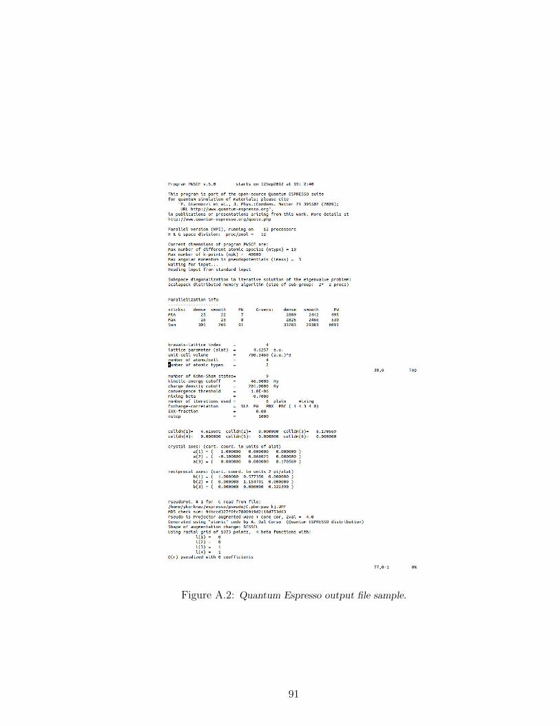
Figure A.2: Quantum Espresso output file sample.

91

92

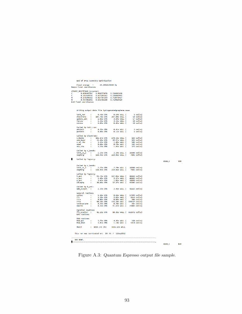
Figure A.3: Quantum Espresso output file sample.

93

Documents

FIRST-PRINCIPLES INVESTIGATION OF FUNCTIONALIZATION OF ... · FIRST-PRINCIPLES INVESTIGATION OF FUNCTIONALIZATION OF GRAPHENE Yaprak Korkmaz M.S. in Physics Supervisor: Prof. Dr