1

Fiscal, Distributional and Efficiency Impacts of Land and Property Taxes

Andrew Coleman & Arthur Grimes *

Paper presented to Tax Session, New Zealand Association of Economists

July 2009

Draft – not for quotation without permission of the authors. Abstract Land taxes are known to be amongst the most efficient forms of taxation since land is an immobile factor; property (capital value) taxes are less efficient owing to the tax on improvements. However there is little international (or New Zealand) evidence regarding the distributional impacts of land and property taxes. Nor is there much New Zealand evidence on their potential fiscal implications or about the taxes’ impacts on asset values and debt positions. We explore impacts that may arise from a range of land and property taxes that differ across certain features (e.g. comprehensiveness and degree of grand-fathering). Both partial and general equilibrium models are used. The results provide a basis for considering alternative taxation options that may be considered domestically. JEL Codes: H21, H22, H24

* Andrew Coleman is Senior Fellow at Motu Economic & Public Policy Research. Arthur Grimes is Senior Fellow at Motu Economic & Public Policy Research and Adjunct Professor at the University of Waikato. The authors thank the New Zealand Treasury for partial funding of the study, together with support from the Marsden Fund of the Royal Society of New Zealand (grant 07-MEP-003, Home Ownership and Neighbourhood Wellbeing) and the Foundation for Research, Science and Technology (programme MOTU0601 Infrastructure) for funding aspects relevant to each programme. Chris Young (Motu) and Trinh Le (NZIER) provided expert assistance with data extraction. Access to the SoFIE data used in this study was provided by Statistics New Zealand in a secure environment designed to give effect to the confidentiality provisions of the Statistics Act, 1975. The results in this study and any errors contained therein are those of the authors, not Statistics New Zealand or of any other organisation.

2

1 Introduction Many developed countries are facing the prospect of significant structural central government budget deficits (IMF, 2009). While not affected as badly as some countries, New Zealand’s budgetary situation has also turned to deficit (New Zealand Government, 2009). These pressures make it sensible to revisit both expenditure decisions and revenue-raising options. This paper addresses aspects of the latter, focusing on land and property taxes. Some economies raise a material proportion of tax revenues by way of land and/or property taxes.1 In New Zealand, local government raises approximately 60% of its revenue requirements through local authority ‘rates’ variously levied on land values or capital values of properties (McCluskey et al, 2006). The central government does not employ such taxes, although their use has been mooted since at least 1844 when Governor FitzRoy attempted (unsuccessfully) to introduce a tax on both land and improvements.2 We analyse fiscal, distributional and efficiency effects of land taxes and/or property taxes. Additional revenues raised through such taxes could be used (and is used in our modelling) to reduce other tax revenues, with expenditures being left unchanged. Thus we are interested in modelling the effects of a fiscally-neutral change to the tax structure. Our analysis covers the effects both of a “land tax” (i.e. a tax on land value) and of a “property tax” (i.e. a tax on capital values of property, being the sum of improvements plus land value).3 For much of the analysis we will be specific about whether we are dealing with a tax solely on land value (a land tax) or on total capital values (property tax). In some cases, where we wish to be more general, we refer to land/property taxes. Certain variants to basic land/property taxes are also explored. In applying the analysis to New Zealand data, we utilise existing valuations (rateable values) performed by Quotable Value New Zealand (QVNZ) for all New Zealand properties. These valuations, which already split capital values into land and improvement values, have an existing statutory basis and are used currently as the base for local authority rates revenues. Our theoretical and empirical work is intended as a purely positive analysis of the effects involved. We make no claims that one taxation regime has net benefits relative to another; rarely is it possible in public policy to achieve a pure Pareto improvement in which no individual is made worse off. We focus instead on elucidating a range of

1 Hong Kong raises over 35% of government revenue from its property base. The property tax rate is currently set at 15% of rental value (less a 20% deduction for maintenance) equating to 0.75% p.a. of property value using a net yield of 5% p.a. (Hong Kong Democratic Foundation, 1996; Hong Kong Government, 2006). 2 FitzRoy’s proposal was to tax country land (wild or cultivated) at 2d per acre per annum, with a tax on houses at a rate of £1 p.a. per room excluding the first three rooms, garrets, outhouses and closets (Goldsmith, 2008). 3 Conceptually, “land value” is best thought of as unimproved land value; i.e. the value prior to any drainage, landscaping, etc. In practice, land incorporates some improvements and this may lead to taxation of “land improvements” even with a land tax; see Franzsen (2009) for discussion of regimes that attempt to tax only unimproved land. In this paper, unless otherwise indicated, we abstract from this complication.

3

impacts that might occur following introduction of a central government land/property tax. We begin with a brief summary of prior treatments of land and property taxes, including previous New Zealand contributions. These contributions can be considered in the context of generally recognised properties of sound taxation systems, including efficiency and distributional (equity) considerations. We follow this summary with a partial equilibrium treatment of the effects of a land/property tax on individual land/property values. While the partial equilibrium analysis helps to cement key concepts, it ignores system-wide effects that may produce quite different results in aggregate. We therefore also adopt a general equilibrium approach to gauge economy-wide results of the introduction of a property tax. The general equilibrium model, designed to reflect key stylised properties of the New Zealand economy, produces some material insights that are not at first apparent from a partial equilibrium approach. The paper’s empirical work assesses fiscal and distributional impacts within New Zealand that might occur following a shift towards land/property taxes. Unless otherwise stated, all property values and related data in the empirical analysis refer to 2006. In part this is due to data availability, but it is also a sensible precaution in an environment where property values first increased and then decreased after that date. Fiscal implications cover a range of possibilities, depending on the breadth of the tax base (e.g. whether the tax is on land or property); whether all land types (residential, industrial, commercial, agricultural, forestry, other) are included equally; whether different rules apply to owner-occupied residential properties versus investor-owned (and/or holiday) properties; whether local authority land and/or “Maori land” is included; etc. We use QVNZ valuations to form each of the tax bases wherever possible. In some cases, where we wish to estimate the value of a more restrictive property definition, we use other estimates of specific values. Our purpose in these calculations is to estimate the quantum of tax revenue that may be raised by certain land and property tax variants, which may then be used to reduce revenues from existing tax sources (e.g. personal income taxes or company taxes). In order to examine distributional impacts, we utilise two separate combinations of data at differing levels of aggregation. In each case, the data relate to the household sector, omitting consideration of wider impacts (i.e. we do not consider distributional implications of changes in the values of agricultural, forestry, industrial and commercial properties). We use census and QVNZ data pertaining to territorial local authorities (TLAs) and area units (AU) that enable us to examine relationships, at these levels of aggregation, between household incomes, land taxes and property taxes. Separately, we use household level data obtained from Statistics New Zealand’s Survey of Family Income and Expenditure (SoFIE) to examine relationships between property values, household incomes, household wealth and other variables that are relevant for distributional considerations.

4

2 Context Taxation reduces the disposable incomes of those paying the tax in order to provide sufficient revenue to meet (central and/or local) government expenditures. As well as reducing overall disposable incomes, the design of the tax system has distributional impacts and generally distorts economic activity relative to activities under a tax-free environment.4 In light of these effects, several properties of ‘good’ tax systems are commonly postulated including: allocative efficiency (minimising “excess burdens” at each point of time); dynamic efficiency (minimising misallocation of resources across time); administrative efficiency and transparency; minimising avoidance/evasion; horizontal equity (equal treatment of people in equal situations); and vertical equity (tax burden rises as ability to pay increases). Land taxes are an ancient form of taxation (Dye and England, 2009) and have commonly been recognised as meeting at least some of the tests for a good tax system. Mill (1865, Book 5, Chapter 2, §5) supported adoption of a land tax, particularly one levied on the increment to land values over and above those at a fixed point in time. His reasoning was that the increment in land values was due to general societal influences and that this increment should therefore form the basis for government revenues required for the upkeep of society. George (1880) expanded on Mill’s reasoning, and favoured a land tax as a form of taxation that does not diminish effort or investment while at the same time taxing private value earned from community efforts. The analytical basis for Mill’s and George’s approach was rooted in the insights of Ricardo (1817) - and before him the physiocrats - that land values impound the rents available to land-owners arising from location-specific factors. Modern spatial economics analyses of urban development and the impacts of new infrastructure investments on land values embody a related analytical approach (Roback, 1982; Haughwout, 2002). The favourable allocative efficiency properties of a land tax may be illustrated with reference to the principles of ‘second-best’ taxation (Ramsey, 1927). In efficiency terms, a first-best tax (e.g. a lump-sum tax) does not alter the structure of production, consumption or investment relative to the untaxed economy. In the absence of a lump-sum tax,5 efficiency requires that the tax system be structured to reproduce, as closely as possible, the static and dynamic outcomes under a lump-sum tax.6 To meet this criterion, tax rates should be graduated to reflect their impact on final allocations. Thus, for efficiency, tax rates should be highest on items that, in equilibrium, will have the least change in quantity in response to the imposition of the tax. Land can be treated as an item that has (virtually) a completely inelastic supply, with the quantity being given by “nature” and so fulfils this criterion.7,8

4 Exceptions may occur in cases where the imposition of a tax corrects for a non-existent (or insufficient) market price for a good that has real resource costs; e.g. a carbon tax. 5 With international migration, even a poll tax cannot be regarded as a lump-sum tax since people can migrate to avoid it. 6 Note that this efficiency objective may clash with distributional (equity) considerations, and hence policy trade-offs may need to be made. 7 This statement embodies slight inaccuracies in cases where reclamation is allowed, or where a tax is levied only on economic land and some land is allowed to revert to non-economic uses after the imposition of a tax (e.g. from marginal farmland to mountain tussock).

5

The allocative efficiency properties of a land tax do not automatically flow through to a property (capital value) tax since improvements (e.g. buildings, walls, drainage, etc) are subject to tax under a property tax system, whereas they are not taxed under a land tax. Thus the supply of improvements is affected by a property tax, resulting in distorted resource allocation (McLeod et al, 2001; p.31).9 Given the existence of the local authority rating system, a central government land/property tax would perform very well in terms of administrative efficiency. All valuations required to provide the tax base are already performed and taxes (rates) are already levied comprehensively on property owners by two levels of government (Territorial Local Authorities and Regional Councils). Thus a central government land/property tax could be added as an adjunct to the current system with virtually no additional administrative cost. Furthermore, the ability to avoid (or evade) the tax is virtually non-existent since the land/property is valued by an independent agency and the land/property is available as collateral in cases of non-payment of tax. Taxation of land/property would extend the central government tax base, not just by taxing an asset that has hitherto not been taxed directly at central government level, but also - and more significantly - by taxing non-New Zealanders. Foreign owners of land/property would be obliged to pay the tax (as they currently do for rates). In practice, as shown in succeeding sections, existing foreign owners of land/property at the time of the tax’s establishment would bear the present discounted value of the future tax stream. One complication of land/property taxes (and of local authority rates) is that some households are “property rich but income poor”; this may particularly be the case for retired households. In these cases, systems already exist within some local authorities whereby rates (tax) payments can be accrued against the value of the property, to be met when the property is sold or from the estate.10 In these cases, government would accrue the tax owed to it and would fund the lost cash-flow through other means (e.g. debt-financing, backed by the accrued tax asset). Distributional impacts of land taxes depend not only on the direct impact of the tax, but also on the nature of other fiscal changes occurring at the same time, as well as on general equilibrium reactions of asset and other prices to the package of tax changes. Plummer (2009) reviews international evidence on distributional impacts of a switch between land and property taxes, finding that area-specific features are important in

8 Accordingly, Milton Friedman considered that “the least bad tax is the property tax on the unimproved value of land” (Blaug, 1980). 9 One consequence is that urban development is likely to be relatively more land-extensive (i.e. sprawling) under a property (capital value) tax system than under a land tax system (Oates and Schwab, 2009). 10 See: Local Government Rates Inquiry Panel (2007) that stated (p.13): “The rates postponement scheme operated by a consortium of councils, which is in effect a home equity release or reverse mortgage scheme limited to rates, and the home equity release or reverse mortgage schemes currently being provided by private sector financial institutions may assist some ratepayers.” McLeod et al (2001; p.28) also noted the importance of such a scheme with respect to cash-flows in relation to their suggested Risk Free Return Method (RFRM) of asset taxation.

6

determining both who gains/loses, and the overall progressivity/regressivity of such a change. The lack of consensus concerning distributional impacts of land/property taxes makes a New Zealand-specific analysis of the effects important if such a tax were to be considered here. We begin such an analysis in this paper. New Zealand is an ideal place in which to examine the impacts of land and property taxes since the country has a long history of implementing each form of tax (Hargreaves, 1991; Dowse and Hargreaves, 1999; Franzsen, 2009). New Zealand local authorities were first authorised to levy a property tax in 1844. McCluskey et al (2006) document local authority practices with land value and capital value taxes (and also on annual rental value, similar in concept to capital value). The Local Government Rates Inquiry Panel (2007) found that 56.1% of New Zealand local government revenue was sourced from property taxes (of various forms) in 2005/06. McLeod et al (2001; p.26) showed that the proportion of taxation raised through property taxes was lower in New Zealand than in Australia or the United States. Taking into account all levels of government (federal, state and local), Grimes (2003) found New Zealand’s share of property taxes in government revenue was relatively low, at 5.7%, compared with a 20 country) OECD average of 8.3%; as a share of GDP, New Zealand’s property tax share was also relatively low at 1.8% compared with the average rate of 2.4%. 3 Partial Equilibrium Effects of a Land Tax 3.1 Outline Initial effects of a change in land/property tax rates can be ascertained through the use of partial equilibrium models of land/property valuations.11 We analyse a number of separate regimes, providing both general results and specific numerical examples. Partial equilibrium calculations, by definition, leave out broader economy-wide effects that may impact back on the market in question (in this case, the property market). We provide one example to show the potential impact of such feedbacks prior to a more comprehensive general equilibrium analysis in the next section. Our main focus in the examples that follow is on the effects of a land tax rather than a property (capital value) tax for the efficiency reasons discussed above. For the numerical examples we use a tax rate of 1% p.a. (i.e. a tax payment of $2,000 p.a. for a land parcel valued at $200,000). We analyse one case with a property (capital value) tax for comparison. In addition to a flat rate tax on land value (the most common form of land tax) we examine two alternatives. The first involves gradual introduction of a land tax over a number of years. Such a tax may be considered if cash-flow impacts of full immediate imposition of such a tax were regarded as problematic. The second involves taxing just the increment of land value above some starting value, as per the tax structure implied by Mill. This option involves several complications, but it is nevertheless still feasible to arrive at valuations for variants of this option. 3.2 Simple Land Tax Consider the purchase price of a plot of land at the end of year i=0 that pays the owner an after-income-tax rental stream of Y(1+π)i in years i=1, …, ∞; π is the annual rate of land 11 The analysis here draws on, and extends, that in Oates and Schwab (2009).

7

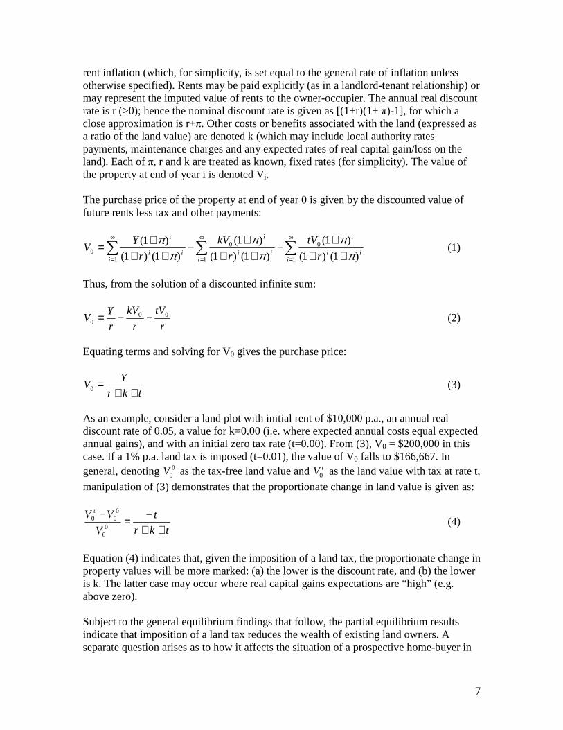
rent inflation (which, for simplicity, is set equal to the general rate of inflation unless otherwise specified). Rents may be paid explicitly (as in a landlord-tenant relationship) or may represent the imputed value of rents to the owner-occupier. The annual real discount rate is r (>0); hence the nominal discount rate is given as [(1+r)(1+ π)-1], for which a close approximation is r+π. Other costs or benefits associated with the land (expressed as a ratio of the land value) are denoted k (which may include local authority rates payments, maintenance charges and any expected rates of real capital gain/loss on the land). Each of π, r and k are treated as known, fixed rates (for simplicity). The value of the property at end of year i is denoted Vi. The purchase price of the property at end of year 0 is given by the discounted value of future rents less tax and other payments:

∑∑∑∞

=

∞

=

∞

= +++

−++

+−

+++=

1

i0

1

i0

1

i

0 )1()1(

)1(

)1()1(

)1(

)1()1(

)1(

iii

iii

iii r

tV

r

kV

r

YV

ππ

ππ

ππ

(1)

Thus, from the solution of a discounted infinite sum:

r

tV

r

kV

r

YV 00

0 −−= (2)

Equating terms and solving for V0 gives the purchase price:

tkr

YV

++=0 (3)

As an example, consider a land plot with initial rent of $10,000 p.a., an annual real discount rate of 0.05, a value for k=0.00 (i.e. where expected annual costs equal expected annual gains), and with an initial zero tax rate (t=0.00). From (3), V0 = $200,000 in this case. If a 1% p.a. land tax is imposed (t=0.01), the value of V0 falls to $166,667. In general, denoting 0

0V as the tax-free land value and tV0 as the land value with tax at rate t,

manipulation of (3) demonstrates that the proportionate change in land value is given as:

tkr

t

V

VV t

++−=

−0

0

000 (4)

Equation (4) indicates that, given the imposition of a land tax, the proportionate change in property values will be more marked: (a) the lower is the discount rate, and (b) the lower is k. The latter case may occur where real capital gains expectations are “high” (e.g. above zero). Subject to the general equilibrium findings that follow, the partial equilibrium results indicate that imposition of a land tax reduces the wealth of existing land owners. A separate question arises as to how it affects the situation of a prospective home-buyer in

8

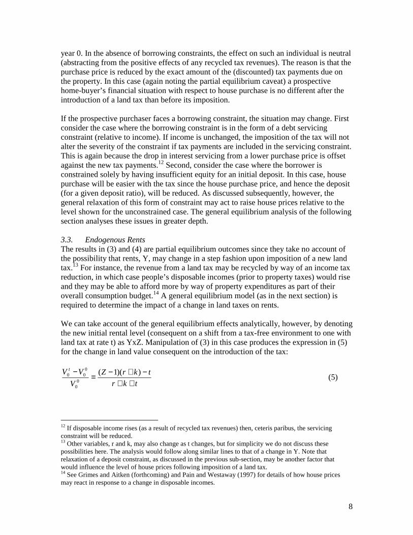
year 0. In the absence of borrowing constraints, the effect on such an individual is neutral (abstracting from the positive effects of any recycled tax revenues). The reason is that the purchase price is reduced by the exact amount of the (discounted) tax payments due on the property. In this case (again noting the partial equilibrium caveat) a prospective home-buyer’s financial situation with respect to house purchase is no different after the introduction of a land tax than before its imposition. If the prospective purchaser faces a borrowing constraint, the situation may change. First consider the case where the borrowing constraint is in the form of a debt servicing constraint (relative to income). If income is unchanged, the imposition of the tax will not alter the severity of the constraint if tax payments are included in the servicing constraint. This is again because the drop in interest servicing from a lower purchase price is offset against the new tax payments.12 Second, consider the case where the borrower is constrained solely by having insufficient equity for an initial deposit. In this case, house purchase will be easier with the tax since the house purchase price, and hence the deposit (for a given deposit ratio), will be reduced. As discussed subsequently, however, the general relaxation of this form of constraint may act to raise house prices relative to the level shown for the unconstrained case. The general equilibrium analysis of the following section analyses these issues in greater depth. 3.3. Endogenous Rents The results in (3) and (4) are partial equilibrium outcomes since they take no account of the possibility that rents, Y, may change in a step fashion upon imposition of a new land tax.13 For instance, the revenue from a land tax may be recycled by way of an income tax reduction, in which case people’s disposable incomes (prior to property taxes) would rise and they may be able to afford more by way of property expenditures as part of their overall consumption budget.14 A general equilibrium model (as in the next section) is required to determine the impact of a change in land taxes on rents. We can take account of the general equilibrium effects analytically, however, by denoting the new initial rental level (consequent on a shift from a tax-free environment to one with land tax at rate t) as YxZ. Manipulation of (3) in this case produces the expression in (5) for the change in land value consequent on the introduction of the tax:

tkr

tkrZ

V

VV t

++−+−=

− ))(1(0

0

000 (5)

12 If disposable income rises (as a result of recycled tax revenues) then, ceteris paribus, the servicing constraint will be reduced. 13 Other variables, r and k, may also change as t changes, but for simplicity we do not discuss these possibilities here. The analysis would follow along similar lines to that of a change in Y. Note that relaxation of a deposit constraint, as discussed in the previous sub-section, may be another factor that would influence the level of house prices following imposition of a land tax. 14 See Grimes and Aitken (forthcoming) and Pain and Westaway (1997) for details of how house prices may react in response to a change in disposable incomes.

9

Using our previous example (Y=$10,000; r=0.05; k=0.00; t=0.01), if Z were 1.2 (i.e. a 20% upward shift in rents consequent on the tax) there would be no change in the purchase price of the land. This result is important in considering the effects of imposing a land tax. In general, if the new tax revenue is used to reduce other taxes, the value of rents will change (most probably upwards, given the increase in disposable incomes) and so a partial equilibrium estimate of the downward effects of the tax on land values may be overstated. 3.4 Property Tax Analysis of the impacts of a land tax on land prices can be extended to the impacts of the introduction of a property tax on property prices (i.e. on the sale price or capital value of the property). In order to model this generally, we allow the tax on land value (t) to differ from the tax on improvements (s), and also allow ‘other’ rates of costs or benefits to differ, with rate k for land and j for improvements. The latter is particularly important since the costs of depreciation/maintenance for improvements is likely to be much higher than that for land. The initial annual rental stream from improvements is denoted M. We denote the year 0 value of the property as H0. Since H equals the value of land plus the value of improvements, we can use the same methods as in (1) – (3) to derive the value of H0 as:

sjr

M

tkr

YH

+++

++=0 (6)

Assuming no changes in Y or M consequent on the introduction of a land or improvements tax (i.e. the partial equilibrium case), we can manipulate (6) to examine the effects of tax changes on initial property value. Analytically, the simplest case is where t=s and k=j in which case the impact of a change in property taxes from zero to t (=s) is given again by equation (4). From the discussion following (4) we know that the higher is k or j, the smaller is the proportionate change in property price following the imposition of a tax. In practice, we expect j>k, possibly for two reasons. The first is that the rate of maintenance costs on improvements is likely to exceed that on land. This explanation is consistent with current tax schedules which treat depreciation on structures differently from depreciation of land. The second is that zoning and/or topographical constraints mean that urban land may be in less elastic supply than improvements, in which case real capital gains expectations for land for urban uses may exceed those for improvements. If it is the case that j>k, the proportionate effect on property prices of the introduction of a property tax (with t=s) will be less than that indicated by (4). We can examine the impacts of the imposition of a land tax only (i.e. s=0) on the overall property price. In practice, this will be the chief indicator of impact for a property owner. Using the same terminological approach as before, we can manipulate (6) to show the proportionate change as:

10

)]/)(())[((

)(00

000

YMkrjrtkr

jrt

H

HH t

++++++−=

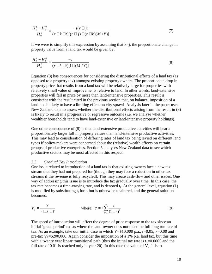
− (7)

If we were to simplify this expression by assuming that k=j, the proportionate change in property value from a land tax would be given by:

)]/(1)[(00

000

YMtkr

t

H

HH t

+++−=

− (8)

Equation (8) has consequences for considering the distributional effects of a land tax (as opposed to a property tax) amongst existing property owners. The proportionate drop in property price that results from a land tax will be relatively large for properties with relatively small value of improvements relative to land. In other words, land-extensive properties will fall in price by more than land-intensive properties. This result is consistent with the result cited in the previous section that, on balance, imposition of a land tax is likely to have a limiting effect on city sprawl. Analysis later in the paper uses New Zealand data to assess whether the distributional effects arising from the result in (8) is likely to result in a progressive or regressive outcome (i.e. we analyse whether wealthier households tend to have land-extensive or land-intensive property holdings). One other consequence of (8) is that land-extensive productive activities will bear a proportionately larger fall in property values than land-intensive productive activities. This may lead to consideration of differing rates of land tax being levied on different land types if policy-makers were concerned about the (relative) wealth effects on certain groups of productive enterprises. Section 5 analyses New Zealand data to see which productive sectors may be most affected in this respect. 3.5 Gradual Tax Introduction One issue related to introduction of a land tax is that existing owners face a new tax stream that they had not prepared for (though they may face a reduction in other tax streams if the revenue is fully recycled). This may create cash-flow and other issues. One way of addressing this issue is to introduce the tax gradually over time. In this case, the tax rate becomes a time-varying rate, and is denoted ti. At the general level, equation (1) is modified by substituting ti for t, but is otherwise unaltered, and the general solution becomes:

τ++=

kr

YV0 where: ∑

∞

= +=

1 )1(ii

i

r

trτ (9)

The speed of introduction will affect the degree of price response to the tax since an initial ‘grace period’ exists where the land-owner does not meet the full long run rate of tax. As an example, take our initial case in which Y=$10,000 p.a., r=0.05, k=0.00 and pre-tax V0=$200,000. Again consider the imposition of a 1% p.a. land tax, but this time with a twenty year linear transitional path (thus the initial tax rate is t1=0.0005 and the full rate of 0.01 is reached only in year 20). In this case the value of V0 falls to

11

$176,858,15 which can be compared with the fall to $166,667 with full immediate introduction. Thus a gradual introduction of the tax alleviates cash-flow issues for existing land-owners in the early years of the tax, and results in a lesser fall in land (and property) values than immediate introduction. The counterpart to these outcomes is that initial tax revenues raised by the tax are reduced, and so there is less land tax revenue to recycle in other forms. 3.6 Incremental Tax Base Another approach to alleviating initial cash-flow impacts of the tax is to levy the tax only on the increments of land value over and above some initial level. This approach is in keeping with the idea mooted by Mill. It escapes the potential “fairness” criticism that existing owners were not aware of the potential tax liability when purchasing the property. By taxing only the increment in property values, the tax, in effect, becomes a form of capital gains tax on property.16 This version of the tax is more complicated to model because even the taxation of incremental value will cause the initial land value to fall by the discounted amount of the future tax stream. Thus the increment above initial (pre-tax) values will disappear for some years until such time as capital gains are sufficient to raise land value back beyond the pre-tax level. In order to model this option effectively, we assume that there is some threshold level of land value, X, that is not taxed, and that all increments above this level are taxed. We assume that X is set such that X≤ tV0 ; thus land values do not fall below the threshold

value even after the imposition of the (incremental) tax. The expression determining land value now becomes:

∑∑∑∞

=

∞

=

∞

= ++−+

−++

+−

+++=

1

i0

1

i0

1

i

0 )1()1(

])1([

)1()1(

)1(

)1()1(

)1(

iii

iii

iii r

XVt

r

kV

r

YV

ππ

ππ

ππ

(10)

which solves as:

))((0 tkrr

rtX

tkr

YV

++++

++=

π (11)

From (11), one can solve for the threshold value that equals the new (lower) level of land prices by equating X with V0, to give:

15 This value is found through numerical solution rather than from a closed form solution. 16 Administratively, however, an incremental land tax is far simpler to implement than an accrual capital gains tax (which can cause major cash-flow problems in particular years for the taxpayer) and does not have the lock-in problems of a capital gains tax on realised capital gains.

12

rttkrr

YrXV

−++++==

))((

)(0 π

π (12)

For our standard example (Y=$10,000; r=0.05; k=0.00; t=0.01) with π=0.02, the threshold value becomes $189,189. Thus even though only increments above the new land value are taxed, land value still falls by 5.4% (given these parameter choices). If π=0.04, the threshold value falls further to $183,673 (an 8.2% fall). Thus as inflation rises, the new market value of land falls, despite only the increment to the land value (above its new initial equilibrium) being taxed. The reason for this result is that the incremental tax considered here is one that taxes nominal capital gains, rather than real capital gains. If only real capital gains were taxed, (i.e. if the threshold was set so that X=00V and indexed at rate (1+π), no tax would be

collected on the inflation component. 3.7 Taxation of “Betterment” Due to Infrastructure Improvements One situation in which real capital gains may arise is where a specific infrastructure investment (or new local amenity) raises local land values (Roback, 1982; Haughwout, 2002; Grimes and Liang, forthcoming). A related situation is where land is rezoned, for instance from agricultural to residential use (Grimes and Liang, 2009). The rise in land values in this situation is sometimes termed “betterment”. Betterment can be captured by the infrastructure investor if that investor owns the land serviced by the new investment;17 otherwise (in the absence of taxation or development levies) it accrues to private land-owners who may not have funded the investment. In this latter situation, (some portion of) betterment can be captured if the rise in land values attributable to the infrastructure investment is taxed.18 In order to differentiate this form of tax from the prior example (in which the inflation component of land value gains is taxed), we concentrate here solely on the taxation of real capital gains. (Formally, this is equivalent to taxing nominal gains and setting π=0 in our analysis.) We consider two alternatives. First, we consider the effectiveness of a general (real) land tax in taxing betterment values. Second, we consider the effectiveness of an incremental (real) land tax for the same purpose. For the first alternative, assume that a land tax (at rate t) is in place and that a specific plot of land earns rent Y p.a. Based on our past derivations the value of the plot is initially given by (3) [i.e. V0=Y/(r+k+t)]. A public infrastructure project is then built that raises the annual rental stream to Y*; thus the new plot value is: V*0=Y*/(r+k+t). In the absence of a land tax, the present discounted value of the extra rents to the land-owner would be (Y*-Y)/(r+k); with a land tax, the difference is reduced to (Y*-Y)/(r+k+t). 17 For an historical example in New Zealand see New Zealand Government Railways Department (1927). 18 In 1870, Sir Julius Vogel, as part of his massive public works scheme, proposed a small betterment tax on private properties that increased in value as a result of the proposed new railway. The proceeds of the tax were intended to part-fund the investment. Woods (1935) documents that the proposed tax was rejected by Parliament, whose “representatives were, in the main, land-owners.” For a review of modern international and New Zealand practices in this respect, see SGS Economics and Planning (2007).

13

Thus, in the latter case, some of the betterment value accrues to government as tax revenue (in this partial equilibrium setting). The amount accruing to government as a result of the interaction of betterment with land taxes (denoted B) is given by:

))((

)*(

tkrkr

YYtB

+++−= (13)

Based on our previous example (r=0.05; k=0.00) and with t variously set to 0.00 and 0.01, the zero tax case produces a betterment value of $20 for every $1 p.a. rise in rents, whereas the 1% land tax case produces an after-tax betterment value to the land-owner of $16.667. A 1% land tax therefore only captures one-sixth of the betterment value in this case. With the second alternative, only real incremental land value is taxed (at rate t). Using previous results, the value of a plot of land that experiences an unexpected rise in land rents from Y to Y* becomes:

tkr

YY

kr

YV

++−+

+= *

0 (14)

The first term on the right hand side of (14) is the existing land value (prior to the rise in rents) which is invariant to the incremental land tax. The second term in (14) reflects the rise in land value consequent on the rental rise. Of this increment, the proportion (r+k)/(r+k+t) accrues to the land-owner while t/(r+k+t) accrues to government. Using the same numerical example as before, if t=0.00, land value rises by $20 for every $1 p.a. rise in land rents; whereas with t=0.01, the land value rise is $16.667; i.e. the same result as for the general land tax case. However, since the real incremental land tax is not levied on existing land values (by definition) or on the inflation component of future rises in land values (also by definition), the tax rate could realistically be set considerably higher than could a general land tax rate. Consider, for instance, a policy that was targeted at taxing real capital gains on land at rate c. That could be achieved through a capital gains tax (at rate c) on the one-off annual capital gain, or it could be achieved by equating the desired rate of capital gains tax with the government’s share of betterment through an annual incremental land tax at rate t where, from the analysis following (14):

)1(

)(

c

ckrt

−+= (15)

For instance, with a desired capital gains tax of 30% and with r=0.05 and k=0.00, an incremental land tax rate of 2.14% p.a. would result in 30% of the real capital gain (in present discounted value terms) accruing to government. Cash-flows from an incremental land value tax would differ from a capital gains tax since the former would be spread over the indefinite future whereas a ‘pure’ capital gains tax is due immediately (within

14

one year) of the capital gain being apparent. In many jurisdictions, cash-flow concerns with regard to the taxpayer means that the capital gain is only payable on realisation of the property, which creates lock-in effects and other complications. These issues are much less problematic in the case of an incremental land tax. 4 General Equilibrium Effects of a Property Tax 4.1 Outline We utilise the model detailed in Coleman (2009) to analyse broader implications of a property tax on the housing market. The model, which extends that of Ortalo-Magné and Rady (2006), is a multi-cohort steady state model in which each cohort chooses its housing type at each stage in life from a range of four options subject to a lifetime budget constraint and a credit constraint. The credit constraint imposes both a minimum deposit requirement on house purchase and a maximum servicing constraint in relation to current income. All mortgages are table mortgages; thus, with a rising income profile over a person’s lifetime, the credit constraint is most likely to bind in earlier years of adulthood. The budget constraint is affected not just by lifetime income (which is set exogenously for each person/family19) and by housing and goods expenditures (which are endogenous) but also by taxation rates. In the baseline model without a property tax, agents face a GST rate of 12.5% and a two-step income tax regime with a lower marginal tax rate of 20% and an upper marginal tax rate of 33% on current incomes. In our simulations, we vary the tax rates, subject to maintenance of a balanced fiscal position. The exogeneity of agents’ incomes means that we do not allow for any production changes as a result of taxation changes. For instance, we do not account for any rise in productivity as a result of shifting from an income tax to a property tax. Our simulations will therefore understate net benefits of such a tax shift if productivity improvements would eventuate from such a tax switch in the actual economy. The four housing choices for each family are, from lowest to highest: (a) share a rental apartment with others; (b) rent an apartment without sharing; (c) live in an owner occupied apartment; (d) live in an owner-occupied house. Utility increases as the family moves up the ladder from (a) to (d). An agent with net savings can either invest in financial assets or in an investment property (apartment) so that returns are equated across the two investments; the latter investment provides the rental stock for categories (a) and (b) above. The supply elasticities for both apartments and houses are set as parameters in the model enabling simulations to differ according to how elastic is the supply of apartments and houses in the model economy. Other important parameters relate to the lifetime income profile, utility from each housing type and from goods consumption, and the specifics of the credit constraint. Because buyers face a table mortgage (i.e. a flat mortgage repayment schedule) an increase in the inflation rate creates conditions in which the credit constraint is more likely to bind; inflation also interacts with the tax system to create a wedge between borrowing and lending rates when inflation is non-zero. We

19 The model can be thought of as pertaining to either a person or a family; we refer to “family” or “agent” in the following.

15

focus on the zero inflation case so as to concentrate on the situation in which inflation does not distort outcomes. We have also conducted simulations with a positive inflation rate (at 2% p.a.) and the broad nature of the reported results are robust to this change. Another important aspect is the nature of bequests in the model. Agents bequeath the value of their apartment/house (if they own one in their final period of life), but do not bequeath financial assets (i.e. they run down their financial wealth to zero by time of death by consuming through their lifetime). This raises the issue of who receives the bequest. Our simulations assume that each agent receives a bequest from someone at the corresponding point in the income scale (i.e. a person at the 75th percentile in his cohort’s income scale receives a bequest from a person who has just died who was also at the 75th percentile in her income scale). Another alternative is that each agent faces an even chance of receiving a bequest or no bequest (though the size of the bequest, if received, again relates to the agent’s place on the income scale). Results from using the two approaches are broadly similar and we solely report the results using the simpler bequest specification. A key assumption that affects our results is the nature of the housing supply elasticity. We simulate the model with two contrasting assumptions. First, we assume that housing supply is perfectly inelastic. This assumption may approximate the case of a land tax that is levied on all unimproved land in the economy. In that case, while the supply of land to housing may not be perfectly inelastic, all land will be affected by the land tax and so there is no wedge created between housing land and agricultural land, and hence no reason to expect land to be reallocated from one use to another.20 Second, we assume that housing supply is elastic, with an elasticity of unity at equilibrium.21 This may be more appropriate for cases either where a tax on improvements is being considered (since new improvements will be forthcoming as long as the value of improvements exceeds the cost of building them22) or where a land or property tax is imposed on housing, with agricultural land taxed at a lower rate (or exempt) and where there are no controls on conversion of land between alternative uses. The inelastic supply case is closest in concept to the assumptions underlying our partial equilibrium examples with exogenous rents.23 Under all sets of assumptions, prices adjust to ensure a steady state equilibrium in the housing market across all types of houses. First, we run the model with a baseline set of parameters in which GST and income tax rates are set as outlined above, with no property tax. We then impose a property tax of 0.5% p.a. on all (owner-occupied and investor-

20 However, where land improvements are taxed, the long run supply of improved land for residential purposes may not be perfectly inelastic, especially in the longer term. 21 This parameter choice is designed to reflect the long run elasticity of dwellings (but not necessarily residential land) with respect to population. 22 Grimes and Aitken (forthcoming). 23 McLeod et al (2001) draw the distinction between the elasticity of supply of improvements and land within their analysis of existing tax benefits for housing. They state (p.97): “in the long term, the supply of housing is highly elastic such that marginal home buyers will still capture material tax benefits. The land upon which houses are built is in fixed supply so that tax benefits arising on this part of the housing asset will be capitalised into land value.”

16

owned) houses.24 In order to ensure fiscal neutrality, we offset the resulting income to government by: (a) reducing GST, or (b) reducing income tax. In the latter case, we reduce income tax rates so that all agents’ income tax payments are reduced proportionately. The model does not include land separately from improvements which is the reason that we describe the new tax as a property tax rather than as a land tax. As discussed above, the inelastic supply case may be closer to a land tax in which all land in the economy is subject to the same tax rate. Other tax variants could be simulated within this model although, being a steady state model, the tax on incremental value and the gradual tax introduction cases (considered in the partial equilibrium analysis), cannot be simulated here. One alternative simulation that we did investigate was to exempt owner-occupied housing from the property tax so that only investment properties were taxed. This resulted in the virtually complete collapse of the rental market. We do not consider this result to be just an artefact of the model; in reality, a distortion of this nature could severely impact on renters and could have major welfare consequences. 4.2 Inelastic Housing Supply Initially we examine the general equilibrium effects of a shift in taxes under the assumption that housing (and apartment) supply is perfectly inelastic. We simulate two tax changes relative to the baseline tax structure. Letting (tl, tu, tg, tp) be the vector of tax rates pertaining to the lower marginal income tax rate, upper marginal income tax rate, GST rate and property tax rate respectively, our baseline model adopts the tax vector (20%, 33%, 12.2%, 0%).25 Table 4.1 (column 1) reports the resulting outcomes for key variables in the model with this tax structure. The price of apartments and houses are set at $238,600 and $394,900 respectively; annual rent of $12,550 represents a rental yield of just over 5% (on the apartment price) which equals the return on financial assets (5%) plus a small allowance for rates and other housing costs. There are slightly fewer dwellings than families, since some agents choose to “flat” (share an apartment) with others; 88% of households own their own home.26 Home-owning households initially borrow to purchase their property resulting in a household gross debt ratio (relative to GDP) of 69%. Many (mainly middle-aged) households hold financial assets with household net financial assets relative to

24 In section 5, we show that, in fiscal revenue terms, a 0.5% property tax is approximately equivalent to a 1% land tax. 25 GST is set as a residual in the model to ensure that the fiscal position is balanced. Technically, this leads to slight variations in the model’s GST rate from the statutory rate in some simulations (including the baseline); the differences are immaterial and do not affect the tenor of the results. 26 Fewer families than this own their own home, since some families double-up by sharing a house; we focus on the “household homeownership rate” rather than the “family homeownership rate” since the former corresponds to the usual measure cited in policy discussion. The homeownership rate here is artificially high relative to the figure for the actual economy, but it is changes in this rate across simulations, rather than its level, that will concern us henceforth.

17

GDP standing at 28.3%. It is changes to these baseline values (rather than the values themselves) that we will be primarily interested in once we alter the tax parameters. Column 2 provides the steady state outcomes for the case where all property is taxed at a rate of 0.5% p.a. and GST is reduced (to 8.8%) in order to leave the fiscal balance unchanged. As in our partial equilibrium example, apartment and house prices both fall by approximately 10%; thus the present discounted value of the tax is impounded in the property price. Accordingly, gross household debt (required to purchase a property) declines and household net financial assets increase. Rents are almost unaffected by the tax switch, being subject to two offsetting forces: First, with an unchanged rental yield, there is pressure for rents to decline since the purchase price of property has declined but, second, the annual tax is passed on to renters, almost exactly offsetting the first effect. The inelastic supply means that the aggregate number of dwellings does not change, while the homeownership rate increases slightly. The latter reflects an easing in the deposit aspect of the credit constraint since the required deposit to purchase a property has decreased with the decline in purchase prices. Column 3 provides the steady state outcomes where income tax rates are reduced when the property tax is introduced, and GST is left (approximately) unchanged. Prices of properties again impound the bulk of the present discounted value of the property tax, although some substitution between houses, apartments and goods consumption leaves house prices (and to a lesser extent, apartment prices) a little above their level in the GST case.27 The homeownership rate again rises slightly relative to the baseline case (for the same reasons as before), debt levels decline and net financial assets of households increase. These results are broadly as expected from our partial equilibrium analysis given the assumption of completely inelastic supply. The debt and net financial asset results are particularly interesting from a macroeconomic perspective. The household balance sheet, inter alia, comprises property as an asset and mortgage debt as a liability. If a tax is introduced that lowers the value of property assets, the offset is a reduction in gross debt and an increase in net financial assets. At a macroeconomic level, debt, at the margin, is financed from offshore. Thus the steady state effect of a reduction in property prices (as a result of a land/property tax) is a reduction in New Zealand’s gross and net offshore debt and a rise in its net international investment position (NIIP).28 As a result, debt servicing costs will be reduced resulting in a sustained rise in the current account balance. Put simply, high domestic property prices for an indebted country raise the portion of the country’s production that is paid annually to foreigners. While macroeconomic benefits might accrue from imposition of a land/property tax, it is important also to analyse welfare changes at the level of the individual family. Since the model is one in which agents maximise lifetime utility subject to constraints, we can use

27 Note that the reduction in GST leads to a less favourable valuation of housing relative to goods consumption than in the income tax reduction case. 28 To the extent that foreigners own some of the property directly, the reduction in the value of their property equity in New Zealand will also lead to an initial rise in the NIIP.

18

the utility outcome for each agent to measure whether utility rises or falls in each case. Furthermore, we can compare the degree of utility changes across the income spectrum to see how welfare changes according to lifetime earnings. Figure 4.1 divides families into deciles according to lifetime incomes. It charts the average steady state change in utility for households in that decile, firstly for the GST-financed land tax (labelled G) and secondly for the income tax-financed land tax (labelled I). The actual levels of the utility changes need not concern us, but the overall utility changes are important; in addition, the patterns across deciles and the comparison of the G versus I changes are instructive. Every decile experiences a substantial improvement in welfare under both financing options. For most deciles, there is little to choose between the income tax or GST options. Some deciles experience greater welfare improvements than others, generally caused by a greater alleviation of the credit constraint for agents at a specific stage of the income spectrum. Agents in the sixth decile experience a particularly large comparative improvement in welfare. Differing parameters on the credit constraint may shift where some of these larger jumps in utility occur, so not too much emphasis should be placed on this latter result. Agents in the first five deciles experience a larger improvement in utility than agents in the top four deciles (under both financing options). Poorer agents are more likely to rent at some stages of their life, and they benefit from the (GST or income) tax reductions, while not having to pay higher rents following the introduction of the property tax. Richer agents are less likely to rent and so gain less. However, being property owners, they benefit from lower house prices since they have to pay lower servicing costs on their mortgages over their lifetimes. This result is the corollary of the reduction at the macroeconomic level in the country’s gross debt servicing bill. How is it that all deciles can benefit from the change when, by assumption, aggregate GDP is unchanged? One reason is that the tax base has been widened to include imputed rentals, thus enabling a broader base, lower rate tax regime to emerge with a reduced overall excess burden caused by taxation. A separate cause is that initial holders of property suffer a reduction in their property wealth as the initial property price falls.29 This once-only welfare cost on a particular generation is reflected in a permanent welfare gain for all future generations who pay lower servicing costs to foreigners given the lower property values. 4.3 Elastic Housing Supply We repeat the same three tax options with the single change to the model that there is elastic supply for both apartments and houses. As discussed previously, this may be an appropriate assumption with regard to improvements (since the cost of supplying improvements is not directly affected by a property tax) and may be appropriate with respect to land if the taxation on housing land is treated differently to agricultural land and land can be shifted between alternative uses. Results are shown in Table 4.2. 29 Given that we are using a steady state model, this cost is not incorporated into our welfare figures.

19

Some results differ substantially from those with perfectly inelastic supply. In particular, the elastic supply assumption means that - compared with the inelastic case - apartment and house prices change by much less relative to baseline under either tax-financing option. Accordingly, rents rise to maintain required rental yields for landlords. This results in annual rents increasing to incorporate virtually the entire annual property tax payment. The increased tax on housing results in a decline in the number of properties in the economy (i.e., under both financing options, more people share a flat than under the baseline case). Furthermore (not shown separately in the table), there is a change in the mix of dwellings, with a substantial decline in the number of houses and an increase in the number of apartments. The household homeownership rate also falls slightly as property increases in cost (once property tax is added to other ownership costs). Nevertheless, as in the inelastic case, the household debt ratio falls driven principally by the change in dwelling mix from houses to apartments and also, in part, by the reduced number of properties against which to borrow. Accordingly, net financial assets again increase. These effects are in the same direction, but are not as strong, as in the inelastic supply case. Figure 4.2 depicts welfare changes by deciles for each financing option with elastic supply. Overall welfare gains are positive but less than in the inelastic case; seven of the ten deciles show a net welfare gain under each tax financing option. With the GST option, the strongest benefit arises for the lowest decile households. This group is most likely to rent and so faces a higher rental bill for a given housing choice; however, they are also more likely to share a house at some stage of their life. The reduction in utility that arises from sharing is more than compensated by the increase in purchasing power that they obtain as a result of the reduced GST rate.30 Other low income deciles also benefit from a reduced GST rate. Higher decile households benefit most when income taxes are reduced consequent on the introduction of the property tax. This result reflects our choice that the income tax reduction is set so that all individuals face the same percentage reduction in income tax payments. Thus higher income individuals gain a greater dollar reduction in taxes than do poorer individuals. Figure 4.2 indicates that it would be possible to design the income tax reduction so that lower (higher) decile individuals had a greater (lower) percentage cut in income tax payments, essentially by cutting the lower (upper) marginal tax rate by more (less) than the cuts that we have adopted. In so doing, all deciles could be made better off through imposition of a property tax offset by an income tax reduction.31 The elastic supply case, modelled in this sub-section, may under-estimate the price effects and over-estimate the rent effects of a tax switch, especially if the tax switch were fully comprehensive and applied only to land. Nevertheless, it usefully indicates the direction of changes that might occur relative to the inelastic case as elasticity of

30 This result could be dependent on the utility attributed to sharing a rental property rather than renting it outright. Therefore not too much emphasis should be placed on this particular outcome. 31 Again it should be noted that we do not account here for any productivity benefits that may accrue, across all income deciles, from a reduction in income taxes.

20

residential land supply increases. This may be especially relevant if a fully comprehensive tax were not adopted and/or if a property tax rather than a land tax were adopted. The elasticity will also vary according to the time period considered; the supply may be highly inelastic in the short-medium term but more elastic in the long term. The outcomes of the inelastic example reflects the basic properties of Ramsey taxation, discussed above, that optimal taxation involves taxing items for which the allocation does not change as a result of the tax. A comprehensive tax on an inelastically supplied commodity therefore results in superior outcomes than a tax on commodities that are in elastic supply. 5 Fiscal Impacts of a Land/Property Tax We use Quotable Value New Zealand (QVNZ) rateable values for 2006 to estimate the tax base upon which a land tax or a property tax could be levied in New Zealand. QVNZ’s rateable values already form the basis for land/property taxes that exist in the form of local authority rates and thus provide a statutory basis for a central government land/property tax. Currently, valuations are updated every three years for most local authorities. Thus using 2006 data, we have valuations for 2004, 2005 and 2006. We set these all onto a 2006 basis by updating the 2004 and 2005 valuations using movements in the national house price index through to 2006.32 House values comprise more than half of all rateable values (for both land and property) across New Zealand. While each class of property and each area will exhibit some idiosyncratic movement relative to this index, we consider that the resulting estimates are sufficiently accurate to assess the overall effects of the introduction of a new tax. Table 5.1 presents the valuation data across several categories. First, we present data for the total of all properties valued across New Zealand (“Total – All properties”). Included in this total are public buildings, public land and conservation forestry. It is unlikely that such properties would be subject to a land/property tax; thus we include a second total (“Total – ECFO”) that excludes the conservation forestry estate and ‘other’ properties (where the latter are mainly public buildings and public land). This total is then decomposed into four groups: Residential; Commercial Forestry; Agriculture; and Industrial/Commercial/Mining. We follow QVNZ’s categories in this decomposition except that we allocate “lifestyle” properties (both vacant and improved) to residential rather than to agriculture. (Lifestyle properties represent 13% of resulting total residential capital value and 56% of resulting agricultural capital value; if lifestyle properties were allocated instead to “agriculture”, they would comprise 36% of total agriculture value.) For each of the major categories listed above, we present data for total land value, total capital value (and improvements separately), the number of assessments (i.e. number of properties in that category), the average land value and capital value per assessment, and the ratio of land value to capital value for that category. The latter calculation is useful in judging how different sectors would be affected by a land tax versus a capital value tax (for a given revenue target).

32 Source: Reserve Bank of New Zealand website.

21

We provide additional information according to ownership definitions. We use central government accounts to obtain figures for central government owned land and property, and Statistics New Zealand data for local government owned property. The residual is attributed to private ownership. Separately, we use Te Puni Kokiri data to itemise the value of land under the aegis of the Maori trustee (i.e. “Maori land”).33 We also use census data to provide a pro rata estimate of residential land and property that is investor-occupied.34 The latter two categories are useful if consideration were given to exempting certain kinds of properties from a tax. The first two ownership categories may effectively be exempted from any land/property tax which is why we list their values here. We cannot deduct their totals directly from “Total-ECFO” since the latter has already deducted the value of public buildings/land and conservation forestry from “Total – All properties”. The deductions in that case totalled $24.9 billion (land value) and $84.1 billion (capital value); these deductions compare with estimated total central and local government holdings of $20 billion (land value) and $51.8 billion (capital value). Estimated central and local government holdings are therefore less than the deductions already applied to the Total category. Hence it is reasonable to consider that the bulk of these deductions pertain to government holdings and so we do not make further deductions for government holdings from the Total-ECFO category. Several key results are apparent from Table 5.1 (where all ratios are specified relative to Total-ECFO unless otherwise noted). First, Residential comprises 65% of all land values and 69% of all capital values. Second, if owner-occupier households were exempt from a tax, the tax base would shrink by approximately 41% (land value) or 43% (capital value). Third, while land-based industries are often regarded as the “backbone” of the economy, Agriculture and Commercial Forestry together comprise just 24% of all land value in the economy, and an even smaller percentage of capital values. Fourth, for both Residential and Industrial/Commercial/Mining, land values comprise around one-half of capital value; by contrast, the ratios for Agriculture and Commercial Forestry are around four-fifths. Thus a single rate proportional land value tax (with no exemptions) would fall more heavily on existing property owners within land-based industries. Fifth, the average Agriculture land value (per assessment) is over five times that for Residential, while the capital value ratio is 3½ times as great. Thus, if each property was owned by a single occupying household, a proportionate tax would hit agricultural-based households considerably harder than it would hit residential households. These results suggest that consideration may be given (under either a land value or a capital value tax) to a differential rate applied to land classified as (and used as) Agriculture or Commercial Forestry. 33 Other forms of Maori-owned land are not included here. However, even with a broader Maori ownership definition, the numbers listed in Te Puni Kokiri’s (2008) “The Maori Asset Base” relating to Maori property are very small relative to the aggregate values for “Total-ECFO”. 34 The remaining housing is owned by an owner-occupier either directly or through a family trust. This calculation assumes that owner-occupied and investor-owned properties are, on average, of equal value. If owner-occupied homes average a higher (lower) value, our pro rata estimate of investor-owned housing will be an over- (under-)estimate.

22

Table 5.2 provides more detail on the Residential sector, being the largest sector in terms of property values. Slightly more than two-thirds of the value lies within the “residential dwelling” category that includes detached and semi-detached houses. The average capital valuation of each assessed property in this category is $380,000 compared with the average assessed value for apartments/etc at $335,000. Owners of lifestyle properties (with improvements) have the highest average assessed values at almost $600,000. The table also shows that the over 90,000 properties currently being held vacant (but potentially usable for residential purposes) have an average land value of $215,000. A land tax at 1% p.a. therefore amounts to a $2,150 p.a. tax on holdings of each property which may encourage the freeing up of such properties for development. Table 5.3 presents potential revenue figures from a hypothetical 1% p.a. land tax. Initially, we use the full “Total-ECFO” tax base from Table 5.1 based on 2006 values. As discussed previously, the tax base may shrink as a result of such a tax; conversely, introduction of such a tax may not be feasible until at least 2011, so property values may have increased relative to 2006 by that time.35 The third column presents estimates of the initial year land tax revenues both for the full Total-ECFO category and for each sector. Estimates are also provided on the basis that certain sectors (or sub-sectors) may be exempted. The fourth column presents estimates of the initial year revenues from a property tax (i.e. on capital values) that raises the same aggregate revenue as a 1% land tax (excluding consideration of any differing movements in land values and improvements). The resulting capital value tax is set at 0.549%. Consistent with Table 5.1, comparison of the two columns demonstrates that a land value tax would raise more from the commercial forestry and agriculture sectors than would a capital value tax, while a capital value tax would raise more from the industrial/ commercial/mining sectors. The residential sector, in aggregate, would pay similar amounts of tax in either case. (In the following section, however, we show that considerable differences would occur within the residential sector.) The complete exclusion of agriculture and forestry from either tax base would lose between 17% and 24% of total revenue; exclusion of owner-occupied residential housing would lose over 40% of revenues. Exclusion of both agriculture/forestry and owner-occupied housing would emasculate the tax base; revenues would amount to just 36% and 40% of the total potential tax base for a land tax or property tax respectively. Table 5.4 provides a 20 year table of estimated revenues for three different land tax cases (property tax cases would be identical given the same assumptions and using a 0.549% capital value tax rate in place of the 1% land value tax rate). We assume that 2011 land values (after imposition of the tax) are the same as for 2006, and we apply the tax to all sectors within Total-ECFO. Column 1 of the table provides the land value tax base if land

35 Property values continued to increase for two years after 2006, followed by some retracement. We make no forecast of property movements between now and 2011. The reader can easily scale property values and tax revenues up or down compared with those in the table.

23

inflation proceeds at a constant rate of 2% p.a. The second column applies the 1% p.a. land tax to this tax base. The third and fourth columns relate to examples from our partial equilibrium discussion. Column 3 models the revenues obtained with a twenty year gradual introduction of the full land tax, where the initial year’s tax rate is set at 0.05%, rising linearly in 0.05% steps each year until 2030 when the full 1% rate is reached. (Thus revenues in year 2030 are identical to those in the previous column, but revenue in earlier years is reduced.) Column 4 models the revenue implications of a 1% land value tax only on the increments to land value over and above the 2011 level. Thus in the first year, no tax is collected. As land inflation raises the value of land, the tax take increases, reaching approximately one-third of the full level after twenty years.36 In all calculations above, we do not separately model the effects on revenues of excluding Maori-trustee land from the tax base. The numbers are too small to result in a material change in revenues. We note, however, that any exemptions (e.g. for Maori-trustee land, owner-occupier housing, agriculture and forestry) creates incentives to reclassify lands into the exempted sectors. Current classification systems are designed to be resistant to such pressures, but the pressures would no doubt increase if tax rates increased. The most difficult dichotomy to police would possibly be any differentiation between owner-occupied and other housing (whether for an exemption or for a differential tax rate).37 6 Distributional Impacts: Community Level Plummer (2009) documents a paucity of data on the distributional effects of both a land tax and a property tax (and of one relative to the other). In part, the difficulty in determining distributional impacts stems from having to place the land/property tax change in the context of an overall tax policy change in order to consider the combined effects of tax changes as one package rather than as individual components. General equilibrium outcomes that may differ from partial equilibrium assessments of outcomes further complicates the task of determining distributional effects. In addition, a decision has to be made regarding whether to concentrate on initial wealth impacts of the policy change or on subsequent cash-flow impacts. Internationally, one of the difficulties of judging distributional impacts of a land tax (combined with any other tax change) is that data on land values are often sketchy. New Zealand has the advantage that it already starts with a statutory basis for assessing land values in addition to capital values, and thus can analyse distributional considerations based on current official valuation methods.

36 Given the comparatively low tax take for a 1% rate when taxing only incremental values (even compared to the 20 year gradual introduction case), consideration could be given to a higher tax rate in the incremental case if greater revenues were sought. 37 In order to police this distinction, one would possibly need a legally binding declaration from the legal owner (each year) that at least one of the legal owners lived in the house as their main residence for the majority of the year. This would raise the issue of whether a family trust met the criterion.

24

Initially we examine distributional impacts at the community level, where “community” is defined initially at the area unit (AU) level. (In section 7, we analyse data at the household level.) Statistics New Zealand divides New Zealand into 1,919 AU’s which can be considered as tightly defined suburbs (for example, Manukau City has 91 AU’s). We use 1,733 of these AU’s (omitting AU’s that have little or no population such as offshore islands or inlets). We also examine results at the territorial local authority level (TLA), with New Zealand divided into 73 TLA’s. For each community (at AU and TLA level), we obtain Statistics New Zealand 2006 census data and QVNZ 2006 valuation data38 for the following variables (with shortened names in brackets):

- median residential dwelling (RD) land value (MLV); - median RD improvements value (MIV); - median RD capital value, i.e. land plus improvements (MCV); - ratio of median RD land value to median RD capital value (MRAT); - median household income (HHY); - homeownership proportion (HOP).39

These data are collected so that we can examine the cross-sectional relationships between dwelling values and each of household income and homeownership rates. We are particularly interested to test the following hypotheses that would indicate that a land/property tax has features reflecting a progressive tax outcome. Relative to a null hypothesis of no relationship, we test the alternative hypotheses that:

- areas with high incomes have high land values per dwelling; - areas with high incomes have high improvement values per dwelling; - areas with high incomes have high capital values per dwelling; - areas with high incomes have high land relative to capital values per

dwelling. If a positive relationship is found when examining the first three hypotheses we can conclude, from our work in sections 3 and 4, that imposition of a land/property tax will, on average, affect the wealth of higher income households more than that of lower income households.40 The fourth hypothesis is a test of the hypothesis that a land tax is more progressive (across householders) than is a property (capital value) tax (McCluskey et al, 2006). We also examine the relationships between homeownership proportions and each of land values, improvement values, capital values and the land/capital value ratio to help infer what effects changes in these variables may have on homeownership prospects.

38 Valuation data relating to 2004 and 2005 are updated to 2006 using the national house price index. 39 I.e. the proportion of dwellings owned by at least one person living in that dwelling or by a family trust involving at least one resident. 40 Strictly, this statement relies on homogeneity of outcomes within each AU (or TLA). By testing the relationships across two spatial scales (AU and TLA) we can examine whether the degree of aggregation significantly affects the results.

25

Our approach involves analysing a sequence of bivariate relationships since we are aiming at uncovering systematic associations between the variables. This approach cannot attribute causality to the relationships, but we can at least ascertain whether observed associations are consistent with certain hypotheses. We begin by examining the relationship between median household income and the housing data. The top half of Table 6.1 presents AU and TLA level estimates in which we regress lnHHY against each of lnMLV, lnMIV, lnMCV and MRAT plus a constant.41 Use of two different spatial scales enables us to check whether results are affected by size of surveyed unit; we can have greater confidence in the applicability of the results to smaller aggregations if the results from these two aggregations are similar. At both AU and TLA levels, median household incomes are positively related to each of median land value, improvement value and capital value. The results are similar across AU and TLA spatial scales, albeit with slightly higher coefficients at the smaller spatial (AU) scale. The implication of these results is that higher income households tend to live in houses that have higher land values, improvements and capital values. A tax on either land value or capital value therefore appears to be broadly progressive. Consistent with results reported by McCluskey et al using 2001 data, we find that higher income households tend to live in areas where houses have relatively high ratios of land value to capital value. The implication of this result is that a land value tax will be more progressive than a capital value tax, using household income as the yardstick for progressivity. While these results reflect the nation-wide relationships, they may be driven by differences that exist chiefly across TLAs (e.g. by city versus rural differences). We can extract this influence by estimating the AU level equations with the inclusion of a dummy variable for each of the 73 TLAs. The reported slope coefficients then solely measure the relationship between household income and the relevant housing variable within (rather than across) TLAs. This set of estimates is provided in the lower portion of the table. Coefficients on the value variables remain similar to those without the TLA dummies, albeit with a smaller estimated slope for the relationship between household income and land values. Once we extract the cross-TLA differences, the ratio of land to capital values is no longer significant. Thus the observed relationship between household incomes and the ratio of land to capital values at a national level appears to be explained by a cross-TLA, rather than a within-TLA, relationship.42 41 We have estimated the relationships using both linear and logarithmic specifications. The two approaches provide similar results; the logged relationships are useful in that they can be interpreted as elasticities and they make more economic sense in relation to the value variables. MRAT is already expressed as a ratio; logging that variable makes less economic sense, so we use the raw variable. 42 This result differs from that in McCluskey et al (2006) who found a significant relationship even with the inclusion of TLA dummies. Their data covered different years and their relationship had a different functional form; further research into these differing results is therefore warranted.

26

Results for equations that regress the homeownership rate against each of the same variables are presented in Table 6.2. Here we find that the TLA spatial scale is too coarse to produce significant results. At the AU level, the estimates imply that homeownership is higher in areas with high land, improvement and capital values, and lower in areas with high land to capital value ratios. These results indicate that homeowners prefer to locate in “better” (more expensive) areas within TLAs. The negative relationship between homeownership and the ratio of land to capital values implies that homeowners tend to have a higher than average ratio of improvements relative to capital value than do landlords. An implication of this result is that a land value tax would, initially at least, impact more heavily on landlords than an owner-occupiers relative to a property tax. 7 Distributional Impacts: Household Level The community level results indicate that household incomes are positively related to land values and capital values. These results are robust across the two spatial scales used to define communities and are robust to inclusion of TLA fixed effects. There is nevertheless the possibility that the aggregation process, even to an area unit level, may result in an inaccurate portrayal of distributional effects at the household level. We use data from Statistics New Zealand’s 2006 wave of the Survey of Family Income and Expenditure (SoFIE), that includes a wealth survey component, to examine distributional issues at the household level. SoFIE is an official longitudinal survey that is designed to be representative of the New Zealand population. The fine-grained nature of questions in SoFIE, together with the weighting procedures that make the responses representative of the entire population, makes this survey an ideal tool to examine tax impacts at a micro level. The SoFIE wealth survey includes data for the capital value of the household’s owner-occupied house in cases where someone in the household owns the house. Also included is the date of valuation; we update all capital values to 2006 using the national House Price Index, as before. Land values are not available within SoFIE, so our analysis here is of the relationship between property values and other variables of interest.43 Our analysis begins with examination of the relationship between household income and the household’s tenancy status (renter44 or owner-occupier) and, for the latter, the household’s owner-occupied property value.45 Table 7.1 presents a matrix of household incomes by house value, with weights accorded to each cell. Household capital values are presented using the following categories (in 2006 $s): 43 To the extent that land values rise more than proportionately with property values, any positive (negative) links between capital values and other variables will be magnified (attenuated) with regard to land values. 44 All households that are not owner-occupiers are henceforth termed ‘renters’. This includes those “renting” from a family trust; i.e. owner-occupation status in the SoFIE analysis does not include people who reside in a family trust-owned home. 45 Additional (investment or holiday) properties are considered separately.

27

(i) $0 [i.e. renter]; (ii) ($0, $150,000]; (iii) ($150,000, $250,000]; (iv) ($250,000, $350,000]; (v) ($350,000, $500,000]; (vi) >$500,000.

Household incomes are presented by quintile, resulting in the following values:

(i) <$25,030; mean: $14,835; (ii) ($25,030, $43,737); mean: $33,717; (iii) ($43,737, $66,782); mean: $54,799; (iv) ($66,782, $100,850); mean: $82,364; (v) >$100,850; mean: $177,159.

Each cell in the table (other than the final row) represents the proportion of households in that income quintile that owns a house within the relevant capital value category (or, if in the first column, rents a house). The final row presents the proportion of the population that is within that capital value category. Thus 43.2% of households do not live in an owner-occupied home. Of the 56.8% of households that are owner-occupiers, most have properties with a capital value between $150,000 and $500,000, i.e. categories (iii)-(v). For the top income quintile, the proportion of homeowners in each category rises as house values rise, whereas for the lowest income quintile, the proportion of homes that are owned are most heavily weighted to houses below $250,000. These observations, which are consistent with the remaining data in the table, suggest a positive relationship between household incomes and property values. We test this relationship more formally by running a (log) regression of household income (lnHY) on capital value (lnCV) for those households that live in an owner-occupied house. The regression, reported below Table 7.1, uses population weights; thus the effective population size represented by the sample is 938,780 households. On average a 1% increase in capital value is associated with a 0.42% increase in household income; this relationship is tightly specified with a 95% confidence interval for the elasticity of 0.378 to 0.463. The estimated elasticity is higher than that estimated with AU data, which in turn is higher than that estimated with TLA data. Thus as the unit of aggregation is reduced, the estimated elasticity for this relationship rises. The SoFIE-based regression results indicate that the initial wealth effect and the subsequent direct cash-flow impact of a property tax will be greater for higher income households than for lower income households. The household-level coefficients can be used to indicate the potential for income tax reductions that would leave typical households (at specified household income levels) with the same cash-flows. We take three households with annual household incomes of $50,000, $75,000 and $100,000 respectively. Using the SoFIE regression relationship, the households would respectively own a house worth $193,929, $508,055 and $1,006,184. A 0.5% p.a. property tax would

28

result in annual tax payments respectively of $970, $2,540 and $5,031, representing 1.9%, 3.4% and 5.0% of pre-tax annual income. A property tax combined with a constant percentage point reduction in income taxes across the board would therefore leave lower income households better off and higher income households worse off than without the tax change (i.e. a move towards greater progressivity).46 These estimates, however, only cover first round cash-flow effects and do not incorporate the effects of tax changes on rents or, more generally, on renters. They nevertheless indicate a potential for reasonable personal tax reductions while at the same time maintaining or enhancing progressivity. The positive relationship between household incomes and capital value of owned homes is mirrored in the rental market. Table 7.2 divides the sample into three categories based on their rental status. Category (i) pays no rent; category (ii) pays rent of up to $6,550 p.a. while category (iii) pays annual rent above this level. One feature of the data is that (a weighted) 71.6% of households pay no rent. This exceeds the 56.8% of households that live in owner-occupied homes. One cause of this difference is likely to be the treatment of family trust-owned homes that do not charge rent to the “tenants” who live in them. Of those who pay rent, a clear gradation is found across incomes between those who pay “high” rents relative to those who pay low rents. The lowest income quintile has fewer people paying high rents than low rents; whereas this is reversed for the higher quintiles and the ratio of high/low rents increases as the household income quintile rises. This result is formalised (below Table 7.2) with a regression of lnHY on (log of) annual rent (lnRENT) for the sub-sample of those who pay a positive value of rent. The slope coefficient of 0.49 is similar to that for the regression of lnHY on lnCV (0.42). The importance of this result is that if a property (or land) tax were to be reflected proportionately in rents, the same progressivity characteristics that apply to owner-occupiers would also apply (and in a similar manner) to renters. The relationships in Tables 7.1 and 7.2 reflect the relationship between housing variables and household incomes. Another way of assessing the distributional effects of a property tax is to examine the relationship between ownership of property and net worth (wealth) rather than income. This information is presented in Table 7.3, relating the quintiles of net worth to capital value (using the same capital value categories as in Table 7.1). The relationship between the two variables is stark. Over 96% of households in the lowest net worth quintile do not own a home. For the top net worth quintile, the proportion of homeowners increases in line with the capital value category. Over 38% of that quintile own a property worth more than $500,000. By contrast, only 6% of the second highest net worth quintile owns a property of at least that value. The figures in the table demonstrate that a property tax would be progressive, not just according to an income measure, but also according to a wealth measure.

46 A greater reduction in top personal tax rates and lesser reduction in bottom personal tax rates would also be possible while retaining a shift to a more progressive tax system.

29

Across the full (weighted) sample, 14.2% of households owns one or more “investment” properties (i.e. a house which is not their primary residence). Ownership of a second house is most concentrated in those who reside in a category (vi) owner-occupied house (i.e. one worth more than $500,000); 31.3% of this group own additional property. This reduces to 19.9% and 16.5%, 10.5% and 9.2% for categories (v), (iv) (iii) and (ii) residents respectively. For owner-occupiers, the impact of a property tax therefore tends to rise according to the value of their primary residence since owners-occupiers who reside in more expensive homes also, on average, have higher exposures to other property assets.47 Separately, we have examined whether there is a relationship between capital value categories and mortgage servicing ratios in order to examine whether a property tax would hit certain owners harder than others in a cash-flow sense. We define the mortgage service ratio (MSR) as mortgage payments/household income, and regress MSR against lnHY (and a constant). We find no significant relationship between the two,48 indicating that owners of high value homes are no more (or less) likely to face cash-flow problems related to mortgage servicing than owners of low value homes if a property tax were introduced. We examine how a property tax might impact on groups of people with differing characteristics. Table 7.4 tabulates the six capital value categories against the number of children in a house, the ethnicity of the highest income earner in the household,49 and the household’s retirement status.50 In each case, the proportion of the relevant group can be compared against the “total” proportion in that capital value category to see in which categories the group is over- or under-represented. Households with more than 3 children are under-represented in the top three capital value categories, and are strongly over-represented in the rental category. A similar, but slightly less marked, result occurs for households with 3 children. The implication of these results is that a tax on property value will tend to impact least on larger families. However, there are two caveats: First, if large families live in expensive rental accommodation, they may face a significant impact of a property tax indirectly through subsequent rental cash outflows (but not through an initial loss of wealth). Second, we cannot be sure how many of the large families live in family-trust-owned properties and thus be in category (i) in the table. From other information, we know that many households in Housing New Zealand Corporation (“state”) houses include at least 3 children; thus it appears that

47 10.6% of “renters” own a non-owner-occupied property; i.e. a similar proportion to those who reside in category (ii) and (iii) houses. Renters have a greater likelihood of residing in an apartment than do house-owners; 20.0% of renters live in an apartment, compared with between 6.0% and 7.2% for each of categories (ii)-(iv) and just 3.7% to 4.4% for categories (v) and (vi). Thus a property tax would impact more on owners of stand-alone homes than on those of apartments. 48 The coefficient on lnHY is 0.0090 with a t-value of 0.75; the equation R2 is 0.0002. 49 In cases where the highest income earner states more than one ethnicity, the variable is prioritised according to the ordering: Pakeha, Maori, Pacific, Asian, Other. 50 A “retired household” is defined as one in which at least one person reports that they are retired and no-one else in the household is working. All other households are included in the “not retired” category.

30

neither of these caveats is likely to over-turn the implication that households with large numbers of children are more likely to live in less expensive (owned or rented) accommodation. “Retired” households are much more likely than other households to own their own property (75.9% of retired households directly own their house compared with 55.7% of non-retired households). They are over-represented in each of the ownership categories relative to the total population. Retired households are therefore more prone to suffering an initial capital value loss than non-retired households upon introduction of a property tax. Furthermore, if a property tax was introduced with an offsetting reduction in income tax rates, it might be expected that many retired households would gain less from the offsetting income tax reduction than households who have members employed in the workforce. A revenue-neutral land or property tax is therefore likely to impact most heavily on the older property-owning population with benefits to the young and, possibly, also to older renters. The impact of a property tax on housing equity (in the capital sense) across age-groups is, however, more complicated. Most retired people fully own their own property (i.e. with no debt attached) whereas younger owners are more likely to have a mortgage (and their share of equity in the house will tend to reduce as the their age reduces). If a tax were introduced that reduced all property values by 10%, those who own a house without debt would lose 10% of their housing equity whereas those who initially had only 10% of the equity in their home (i.e. who had a 90% loan to value ratio) would lose their entire housing equity. In this sense, young homeowners would face greater losses, on average, than older homeowners.51 Conversely, in a present value sense, they would have more to gain from an offsetting reduction in income taxes. This illustrates that it is important also to consider the full life-cycle consequences of a switch in tax policy when considering distributional implications. The Maori and Pacific populations are greatly under-represented in ownership categories (iii) – (vi), and Pacific families are also under-represented in category (ii). Correspondingly, both are strongly over-represented in the rental category. Both populations will therefore suffer significantly less initial capital value loss than the rest of the population upon introduction of a land/property tax. Furthermore, if their rental houses are generally in low capital value areas, they will face smaller rental rises (in dollar terms) than renters in higher value suburbs. The overall effect of a switch to a property tax from other tax bases on the Maori/Pacific population would, however, depend on what offsetting tax changes were being made. For instance, a reduction solely in the top marginal tax rate may result in a disadvantageous outcome for these population groups, whereas a cut to lower marginal tax rates may result in an overall improvement. The overall tax incidence on particular household and

51 This also raises an issue that introduction of a land/property tax would reduce the collateral that borrowers have in a house, potentially creating riskier exposures for lenders on existing loans (but not on new loans made after the introduction of the tax). This is a purely transitional issue, but potentially a major one not just for home loans but also for loans to productive enterprises, especially in land-based industries.

31

population groups, and the general equilibrium impacts of changes on overall prices in the economy, are important factors to consider for all of the cases that we have examined in this section. 8 Conclusions The fiscal outlook for New Zealand, while not as parlous as in many countries, is still such that some action on fiscal policy is required. Our focus is on the potential for actions on the taxation side that may involve a land tax or a property (capital value) tax. We examine whether significant fiscal revenues could be raised through such taxes. We also examine the effects of a fiscally neutral switch towards land/property taxes away from other tax streams. One reason for focusing on the potential addition of a land tax to the central government’s fiscal armoury is that such a tax has favourable efficiency properties relative to other taxation options. To a first order approximation, the economy’s supply of land is fixed and a tax therefore does not alter the aggregate allocation of this resource. Landowners must pay the tax wherever they are located and whatever the land is used for. By contrast, consumption and income taxes distort allocations by altering labour supply, investment and savings choices and even a poll tax can affect the allocation of resources via migration decisions. Unlike a land tax, a property tax distorts behaviour by changing the net return on improvements, so impacting on investment in structures and other improvements. A switch of some of the existing tax burden from distorting taxes to a land tax may be considered if improvements in allocative efficiency, and thence per capita incomes, are sought. A tax on land could have non-trivial effects both on aggregate fiscal revenues and on individual households and firms (including farms). On the fiscal front, using 2006 figures, we show that a 1% p.a. tax on all non-government land could raise approximately $4.6 billion annually (rising to $6.7 billion annually by 2030 with 2% p.a. land inflation). To place these numbers in perspective, $4.6 billion represents 20% of all income tax revenue forecast for 2009/10. The top personal tax rate of 38% applies above an income threshold of $70,000 p.a. Total income tax revenue raised on those earning above this figure is forecast to be $9.8 billion for 2009/10. If the top personal tax rate were reduced to 33%, the direct loss in income tax would be $491 million, which represents just 11% of the revenue from a 1% p.a. land tax. While a 1% p.a. land tax could result in significant fiscal revenues - so enabling material reductions in other tax rates - it would also have other major effects and its impact would fall more heavily on some sectors of society than on others. One currently untaxed sector that it would fall on is foreign-domiciled owners of New Zealand property, who otherwise pay no income tax and who pay no GST if they do not purchase goods and services in New Zealand. A shift to a land tax would therefore widen the tax base not just in terms of the base of assets on which tax is raised but also in terms of the number of people (i.e. non-New Zealand residents) who become taxpayers. The tax paid by non-New Zealanders contributes a net benefit to the country that exists over and above any efficiency (productivity) benefits that might accrue from the tax shift.

32

The overall effects of a switch to land/property taxes would depend both on what other tax changes are made at the same time (e.g. to GST or income tax) and on the structure of the economy (which determines general equilibrium prices and allocations). Our partial and general equilibrium analyses (sections 3 and 4) demonstrate that certain key parameters (e.g. housing supply elasticities) and the exact nature of the tax (e.g. land versus property tax, incremental versus flat tax, etc) will lead to different outcomes. We therefore cannot be definitive about the overall impacts of a land/property tax. Nevertheless, we can use the foregoing analysis to make some informed judgements about the effects of certain tax policy options under different circumstances. Consider the effects of a comprehensive flat land/property tax funded by a proportionate reduction in income taxes. In this case, with inelastic supply, we may expect land/property prices to fall with rents remaining broadly unchanged. The present discounted value of the tax is effectively reflected in the initial price of the land/property; rents remain unaffected since the tax (which landlords indirectly forward to renters) is offset by the reduced rent required to yield a market return on the reduced initial value of the property. With elastic supply, rents rise since the change in supply means that prices do not fall by the full present discounted value of the tax while the tax is still shifted to renters. In this latter case, the owner-occupancy rate falls slightly as owners’ housing costs rise; in the former (inelastic) case, the owner-occupancy rate rises slightly as more people are able to afford (cheaper) houses despite the housing tax requirements. In all our general equilibrium simulations, aggregate indebtedness of the economy declines with the introduction of a land/property tax, essentially because New Zealanders borrow less to finance domestic property holdings. At a conceptual level, the value of New Zealanders’ housing assets and liabilities fall but, at the margin, the liabilities are sourced from foreign savers and a land/property tax reduces the amount of foreign capital that must be borrowed to fund domestic property. Owners of existing property would incur a loss of wealth following introduction of a land/property tax unless there were perfectly elastic supply. Even in this latter case, if the owners retained the property they would face the present discounted value of the future land/property tax flow (although of course they would also be in receipt of tax reductions from other sources). With a flat land/property tax, the wealth loss would be proportionate to the existing value of land/property. Owners of land-extensive residential properties (including lifestyle properties), farms and forests would be liable for the largest losses in proportion to their property holdings if a land tax were introduced (since improvements would not be taxed in that case). Those with no property holdings would not face an immediate wealth loss. The effect on their rents would depend on the supply elasticity; the less elastic is supply, the less that rents would rise following introduction of the tax. In relation both to current income and current wealth, each of a land and a property tax would tend to be broadly progressive, with higher income (and higher wealth) households tending to bear the greatest burden of a new tax.52 The retired cohort would be more 52 However overall progressivity would depend crucially on the nature of other offsetting taxation changes.

33

likely than younger cohorts to incur a wealth loss given the higher initial value of their housing assets. They would also likely face an increased overall tax burden if a land/property tax was matched by an income tax reduction, simply because their incomes tend to be low in relative terms. Younger cohorts would face reduced current and future income taxes that, on balance, would more than make up for their higher lifetime land tax payments. Wealth losses would tend to be concentrated more upon Pakeha and Asian communities than on Maori and Pacific communities given the low rates of homeownership amongst these latter two ethnic groups. Households with three or more dependent children, on average, would suffer lower wealth losses than households with fewer or no children given existing homeownership patterns. Variants of a flat land tax could be envisaged if a different balance of outcomes was wanted. For instance, if cash-flows amongst already retired households was of key concern, a land tax could be levied only on the increment of land value above some base level or the tax could be introduced with a gradual increase in the tax rate over time. If the financial situation of farmers was of particular concern, a reduced rate on farmland (as defined by an independent body such as QVNZ) could be considered. For a number of reasons (including maintaining the viability of the rental market) it is difficult to see exemption of owner-occupied homes being a viable policy option. We have not modelled the productivity impacts of a switch away from income taxes to a land (or property) tax. Results from the wider tax literature53 indicate that the reduction in distortions to labour supply and investment resulting from lower personal and company tax rates could be expected to lead to some improvement in labour productivity and hence per capita living standards. It appears that fiscal revenues can therefore be enhanced at the same time as reducing excess burdens caused by distortionary taxation. While these aspects favour a land tax, distributive aspects of such a tax will remain a central issue in considering its merits. We make no claims as to which distributive concerns should prevail. Instead, our empirical and modelling results are intended to provide assistance to policy-makers in considering whether certain sets of tax changes result in acceptable trade-offs in order to achieve the fiscal and efficiency enhancements potentially on offer.

53 For instance, see Kneller et al (1999) and Bleaney et al (2001).

34

References Blaug, Mark. 1980. ‘Review of Robert V. Andelson: Critics of Henry George: A Centenary Appraisal of their Strictures on Progress and Poverty’, Economica, New Series, 47, no. 188, 471-472. Bleaney, Michael, Norman Gemmell & Richard Kneller. 2001. ‘Testing the Endogenous Growth Model: Public Expenditure, Taxation, and Growth over the Long Run’, Canadian Journal of Economics, 34(1), 36-57. Coleman, Andrew. 2009. Potential Long Term Effects of Residential Capital Gains Taxes, paper presented to New Zealand Association of Economists conference, Wellington, July. Dowse, G & R. Hargreaves. 1999. ‘Rating Systems in New Zealand’, in W. J. McCluskey (ed.) Property Tax: An International Comparative Review, UK: Ashgate Publishing. Dye, Richard F. & Richard W. England (eds). 2009. Land Value Taxation: Theory, Evidence and Practice, Cambridge, Mass.: Lincoln Institute of Land Policy. Dye, Richard F. & Richard W. England. 2009. ‘The Principles and Promises of Land Value Taxation’, in: Dye, Richard F. & Richard W. England (eds), op. cit., 3-10. Franzsen, Riel. 2009. ‘International Experience’, in: Dye, Richard F. & Richard W. England (eds), op. cit., 28-47. George, Henry. 1880. Progress and Poverty, New York: D. Appleton and Co. Goldsmith, Paul. 2008. We Won, You Lost. Eat That!, Auckland: David Ling Publishing. Grimes, Arthur. 2003. "Economic Growth and the Size and Structure of Government: Implications for New Zealand", New Zealand Economic Papers, 37(1), 151-174. Grimes, Arthur & Andrew Aitken. Forthcoming. ‘Housing Supply, Land Costs and Price Adjustment’, Real Estate Economics. Grimes, Arthur & Yun Liang. 2009. ‘Spatial Determinants of Land Prices: Does Auckland's Metropolitan Urban Limit Have an Effect?’, Applied Spatial Analysis and Policy, 2, 23-45 Grimes, Arthur & Yun Liang. Forthcoming. ‘Bridge to Somewhere: Valuing Auckland’s Northern Motorway Extensions’, Journal of Transport Economics and Policy. Hargreaves, R. 1991. ‘Is Site Value Still an Appropriate Basis for Property Taxation? In: International Conference on Property Taxation and its Interaction with Land Policy, Cambridge, Mass: Lincoln Institute of Land Policy

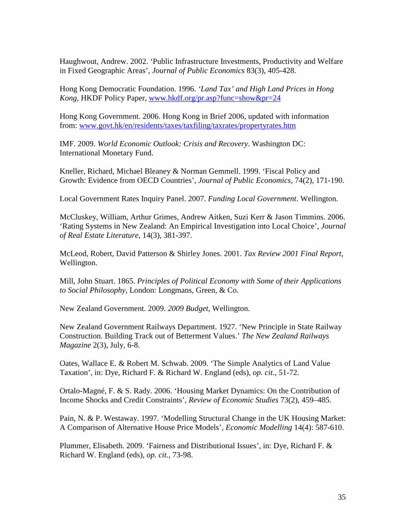
35

Haughwout, Andrew. 2002. ‘Public Infrastructure Investments, Productivity and Welfare in Fixed Geographic Areas’, Journal of Public Economics 83(3), 405-428. Hong Kong Democratic Foundation. 1996. ‘Land Tax’ and High Land Prices in Hong Kong, HKDF Policy Paper, www.hkdf.org/pr.asp?func=show&pr=24 Hong Kong Government. 2006. Hong Kong in Brief 2006, updated with information from: www.govt.hk/en/residents/taxes/taxfiling/taxrates/propertyrates.htm IMF. 2009. World Economic Outlook: Crisis and Recovery. Washington DC: International Monetary Fund. Kneller, Richard, Michael Bleaney & Norman Gemmell. 1999. ‘Fiscal Policy and Growth: Evidence from OECD Countries’, Journal of Public Economics, 74(2), 171-190. Local Government Rates Inquiry Panel. 2007. Funding Local Government. Wellington. McCluskey, William, Arthur Grimes, Andrew Aitken, Suzi Kerr & Jason Timmins. 2006. ‘Rating Systems in New Zealand: An Empirical Investigation into Local Choice’, Journal of Real Estate Literature, 14(3), 381-397. McLeod, Robert, David Patterson & Shirley Jones. 2001. Tax Review 2001 Final Report, Wellington. Mill, John Stuart. 1865. Principles of Political Economy with Some of their Applications to Social Philosophy, London: Longmans, Green, & Co. New Zealand Government. 2009. 2009 Budget, Wellington. New Zealand Government Railways Department. 1927. ‘New Principle in State Railway Construction. Building Track out of Betterment Values.’ The New Zealand Railways Magazine 2(3), July, 6-8. Oates, Wallace E. & Robert M. Schwab. 2009. ‘The Simple Analytics of Land Value Taxation’, in: Dye, Richard F. & Richard W. England (eds), op. cit., 51-72. Ortalo-Magné, F. & S. Rady. 2006. ‘Housing Market Dynamics: On the Contribution of Income Shocks and Credit Constraints’, Review of Economic Studies 73(2), 459–485. Pain, N. & P. Westaway. 1997. ‘Modelling Structural Change in the UK Housing Market: A Comparison of Alternative House Price Models’, Economic Modelling 14(4): 587-610. Plummer, Elisabeth. 2009. ‘Fairness and Distributional Issues’, in: Dye, Richard F. & Richard W. England (eds), op. cit., 73-98.

36

Ramsey, F. P. 1927. ‘A Contribution to the Theory of Taxation’, The Economic Journal, 37, 47-61. Ricardo, David. 1817. On the Principles of Political Economy and Taxation, London: John Murray. Roback, Janet. 1982. ‘Wages, Rents and the Quality of Life’, Journal of Political Economy 90, 1257-1278. SGS Economics and Planning. 2007. Value Capture Mechanisms: International Models and their Relevance to New Zealand, Wellington: Ministry for the Environment. Woods, N.S. 1935. ‘The Birth of Our Railways - The Great Public Works Policy of 1870. Part II” The New Zealand Railways Magazine 10(2), May, 43-44.

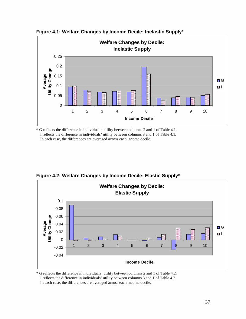
37

Figure 4.1: Welfare Changes by Income Decile: Inela stic Supply*

Welfare Changes by Decile:Inelastic Supply

0

0.05

0.1

0.15

0.2

0.25

1 2 3 4 5 6 7 8 9 10

Income Decile

Ave

rage

Util

ity C

hang

e

G

I

* G reflects the difference in individuals’ utility between columns 2 and 1 of Table 4.1. I reflects the difference in individuals’ utility between columns 3 and 1 of Table 4.1. In each case, the differences are averaged across each income decile. Figure 4.2: Welfare Changes by Income Decile: Elast ic Supply*

Welfare Changes by Decile:Elastic Supply

-0.04

-0.02

0

0.02

0.04

0.06

0.08

0.1

1 2 3 4 5 6 7 8 9 10

Income Decile

Ave

rage

U

tility

Cha

nge

G

I

* G reflects the difference in individuals’ utility between columns 2 and 1 of Table 4.2. I reflects the difference in individuals’ utility between columns 3 and 1 of Table 4.2. In each case, the differences are averaged across each income decile.

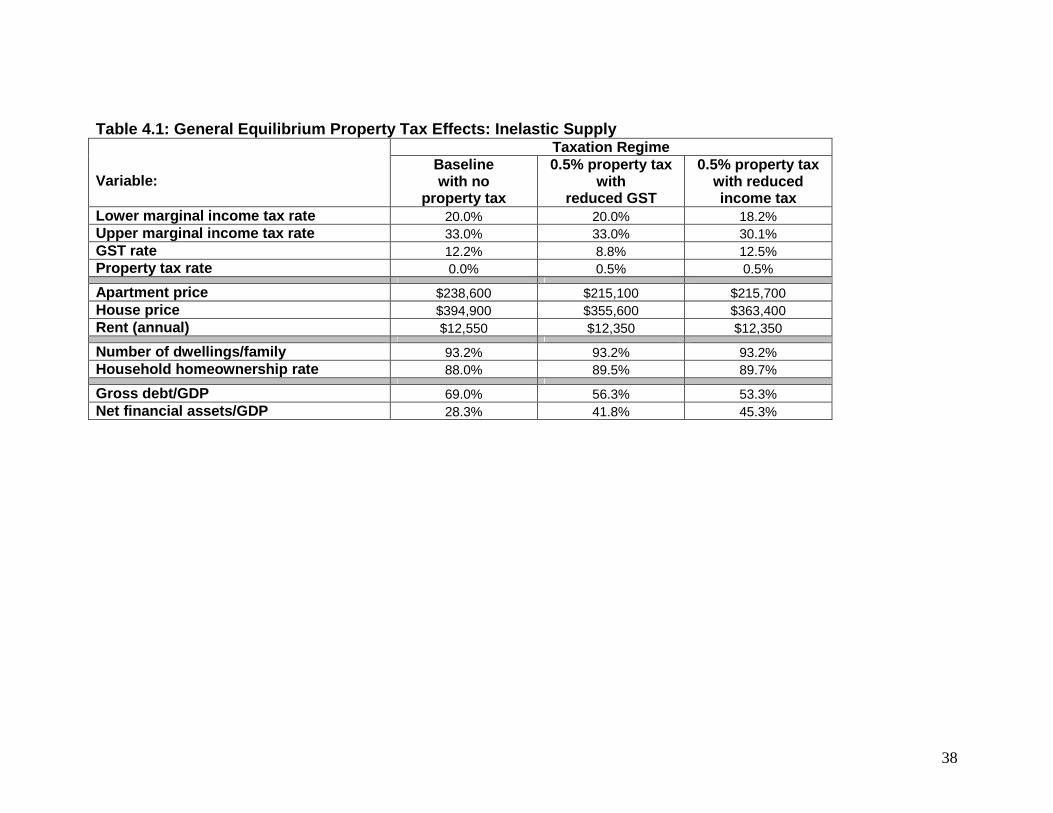
38

Table 4.1: General Equilibrium Property Tax Effects : Inelastic Supply Taxation Regime

Variable:

Baseline with no

property tax

0.5% property tax with

reduced GST

0.5% property tax with reduced income tax

Lower marginal income tax rate 20.0% 20.0% 18.2% Upper marginal income tax rate 33.0% 33.0% 30.1% GST rate 12.2% 8.8% 12.5% Property tax rate 0.0% 0.5% 0.5%

Apartment price $238,600 $215,100 $215,700 House price $394,900 $355,600 $363,400 Rent (annual) $12,550 $12,350 $12,350

Number of dwellings/family 93.2% 93.2% 93.2% Household homeownership rate 88.0% 89.5% 89.7%

Gross debt/GDP 69.0% 56.3% 53.3% Net financial assets/GDP 28.3% 41.8% 45.3%

39

Table 4.2: General Equilibrium Property Tax Effects : Elastic Supply Taxation Regime

Variable:

Baseline with no

property tax

0.5% property tax with

reduced GST

0.5% property tax with reduced income tax

Lower marginal income tax rate 20.0% 20.0% 18.2% Upper marginal income tax rate 33.0% 33.0% 30.1% GST rate 12.3% 9.0% 12.6% Property tax rate 0.0% 0.5% 0.5%

Apartment price $225,300 $221,700 $222,000 House price $384,500 $376,100 $378,000 Rent (annual) $11,850 $12,800 $12,700

Number of dwellings/family 93.9% 92.4% 92.5% Household homeownership rate 90.0% 89.7% 88.3%

Gross debt/GDP 60.3% 55.0% 56.9% Net financial assets/GDP 30.9% 38.4% 41.9%

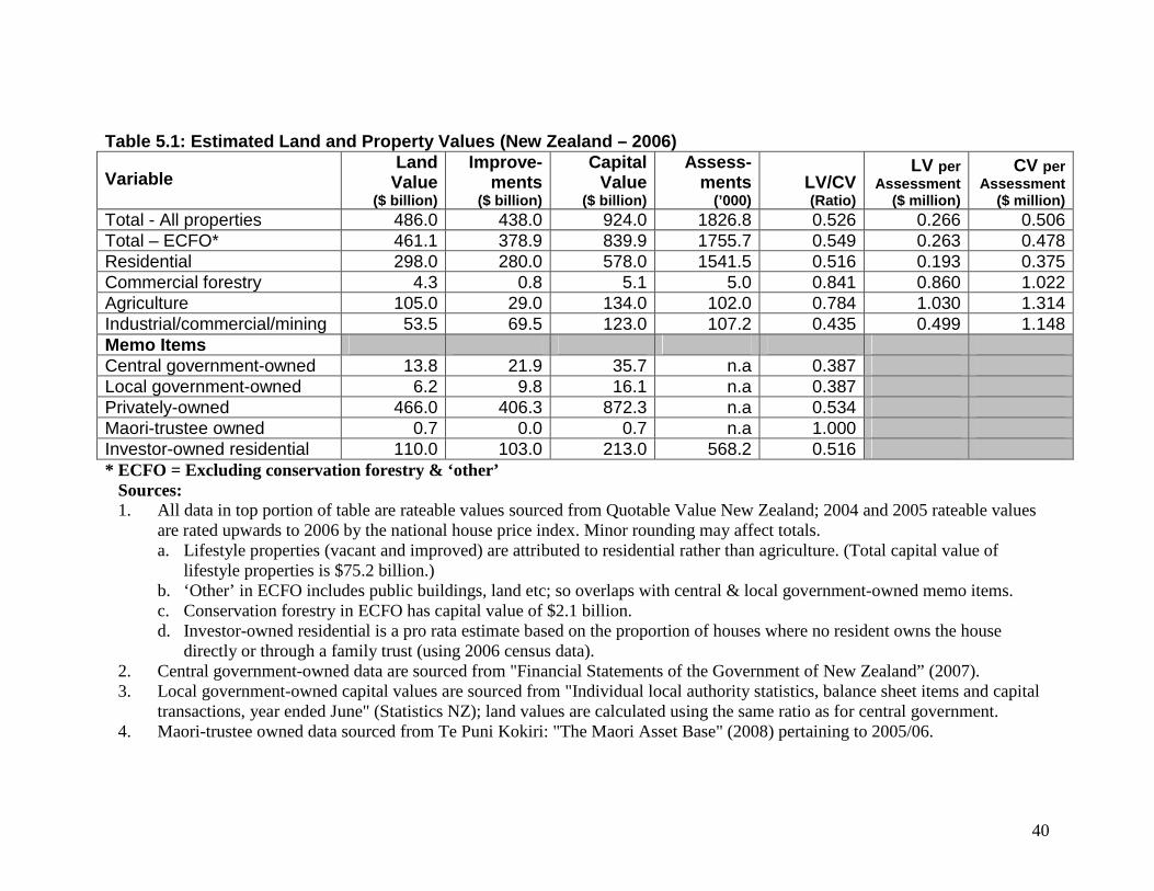
40

Table 5.1: Estimated Land and Property Values (New Zealand – 2006)

Variable

Land Value

($ billion)

Improve- ments

($ billion)

Capital Value

($ billion)

Assess- ments

(’000) LV/CV (Ratio)

LV per Assessment

($ million)

CV per Assessment

($ million) Total - All properties 486.0 438.0 924.0 1826.8 0.526 0.266 0.506 Total – ECFO* 461.1 378.9 839.9 1755.7 0.549 0.263 0.478 Residential 298.0 280.0 578.0 1541.5 0.516 0.193 0.375 Commercial forestry 4.3 0.8 5.1 5.0 0.841 0.860 1.022 Agriculture 105.0 29.0 134.0 102.0 0.784 1.030 1.314 Industrial/commercial/mining 53.5 69.5 123.0 107.2 0.435 0.499 1.148 Memo Items Central government-owned 13.8 21.9 35.7 n.a 0.387 Local government-owned 6.2 9.8 16.1 n.a 0.387 Privately-owned 466.0 406.3 872.3 n.a 0.534 Maori-trustee owned 0.7 0.0 0.7 n.a 1.000 Investor-owned residential 110.0 103.0 213.0 568.2 0.516 * ECFO = Excluding conservation forestry & ‘other’ Sources:

1. All data in top portion of table are rateable values sourced from Quotable Value New Zealand; 2004 and 2005 rateable values are rated upwards to 2006 by the national house price index. Minor rounding may affect totals. a. Lifestyle properties (vacant and improved) are attributed to residential rather than agriculture. (Total capital value of

lifestyle properties is $75.2 billion.) b. ‘Other’ in ECFO includes public buildings, land etc; so overlaps with central & local government-owned memo items. c. Conservation forestry in ECFO has capital value of $2.1 billion. d. Investor-owned residential is a pro rata estimate based on the proportion of houses where no resident owns the house

directly or through a family trust (using 2006 census data). 2. Central government-owned data are sourced from "Financial Statements of the Government of New Zealand” (2007). 3. Local government-owned capital values are sourced from "Individual local authority statistics, balance sheet items and capital

transactions, year ended June" (Statistics NZ); land values are calculated using the same ratio as for central government. 4. Maori-trustee owned data sourced from Te Puni Kokiri: "The Maori Asset Base" (2008) pertaining to 2005/06.

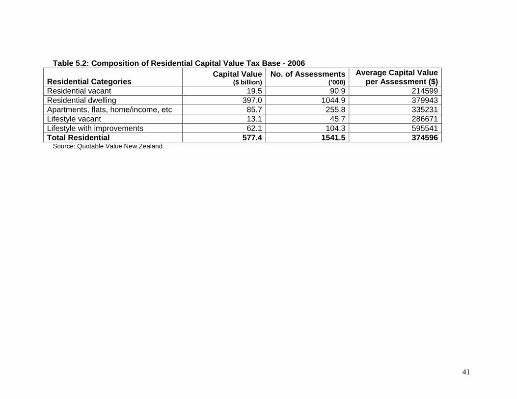
41

Table 5.2: Composition of Residential Capital Value Tax Base - 2006

Residential Categories Capital Value

($ billion) No. of Assessments

(’000) Average Capital Value

per Assessment ($) Residential vacant 19.5 90.9 214599 Residential dwelling 397.0 1044.9 379943 Apartments, flats, home/income, etc 85.7 255.8 335231 Lifestyle vacant 13.1 45.7 286671 Lifestyle with improvements 62.1 104.3 595541 Total Residential 577.4 1541.5 374596

Source: Quotable Value New Zealand.

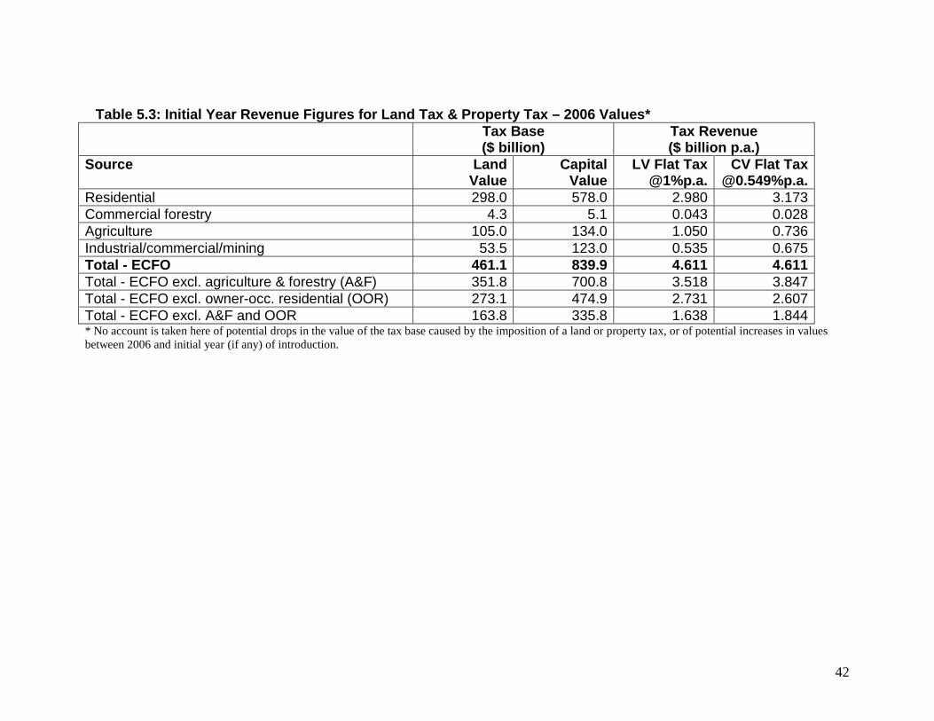
42

Table 5.3: Initial Year Revenue Figures for Land Ta x & Property Tax – 2006 Values*

Tax Base ($ billion)

Tax Revenue ($ billion p.a.)

Source

Land Value

Capital Value

LV Flat Tax @1%p.a.

CV Flat Tax @0.549%p.a.

Residential 298.0 578.0 2.980 3.173 Commercial forestry 4.3 5.1 0.043 0.028 Agriculture 105.0 134.0 1.050 0.736 Industrial/commercial/mining 53.5 123.0 0.535 0.675 Total - ECFO 461.1 839.9 4.611 4.611 Total - ECFO excl. agriculture & forestry (A&F) 351.8 700.8 3.518 3.847 Total - ECFO excl. owner-occ. residential (OOR) 273.1 474.9 2.731 2.607 Total - ECFO excl. A&F and OOR 163.8 335.8 1.638 1.844 * No account is taken here of potential drops in the value of the tax base caused by the imposition of a land or property tax, or of potential increases in values between 2006 and initial year (if any) of introduction.

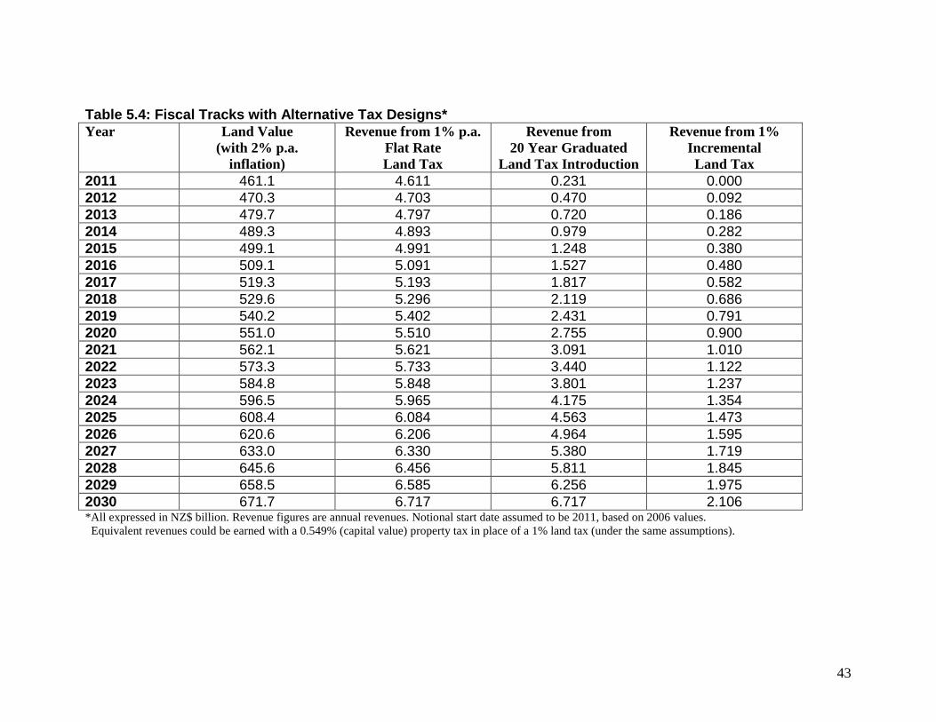
43

Table 5.4: Fiscal Tracks with Alternative Tax Desig ns* Year Land Value

(with 2% p.a. inflation)

Revenue from 1% p.a. Flat Rate Land Tax

Revenue from 20 Year Graduated

Land Tax Introduction

Revenue from 1% Incremental Land Tax

2011 461.1 4.611 0.231 0.000 2012 470.3 4.703 0.470 0.092 2013 479.7 4.797 0.720 0.186 2014 489.3 4.893 0.979 0.282 2015 499.1 4.991 1.248 0.380 2016 509.1 5.091 1.527 0.480 2017 519.3 5.193 1.817 0.582 2018 529.6 5.296 2.119 0.686 2019 540.2 5.402 2.431 0.791 2020 551.0 5.510 2.755 0.900 2021 562.1 5.621 3.091 1.010 2022 573.3 5.733 3.440 1.122 2023 584.8 5.848 3.801 1.237 2024 596.5 5.965 4.175 1.354 2025 608.4 6.084 4.563 1.473 2026 620.6 6.206 4.964 1.595 2027 633.0 6.330 5.380 1.719 2028 645.6 6.456 5.811 1.845 2029 658.5 6.585 6.256 1.975 2030 671.7 6.717 6.717 2.106 *All expressed in NZ$ billion. Revenue figures are annual revenues. Notional start date assumed to be 2011, based on 2006 values. Equivalent revenues could be earned with a 0.549% (capital value) property tax in place of a 1% land tax (under the same assumptions).

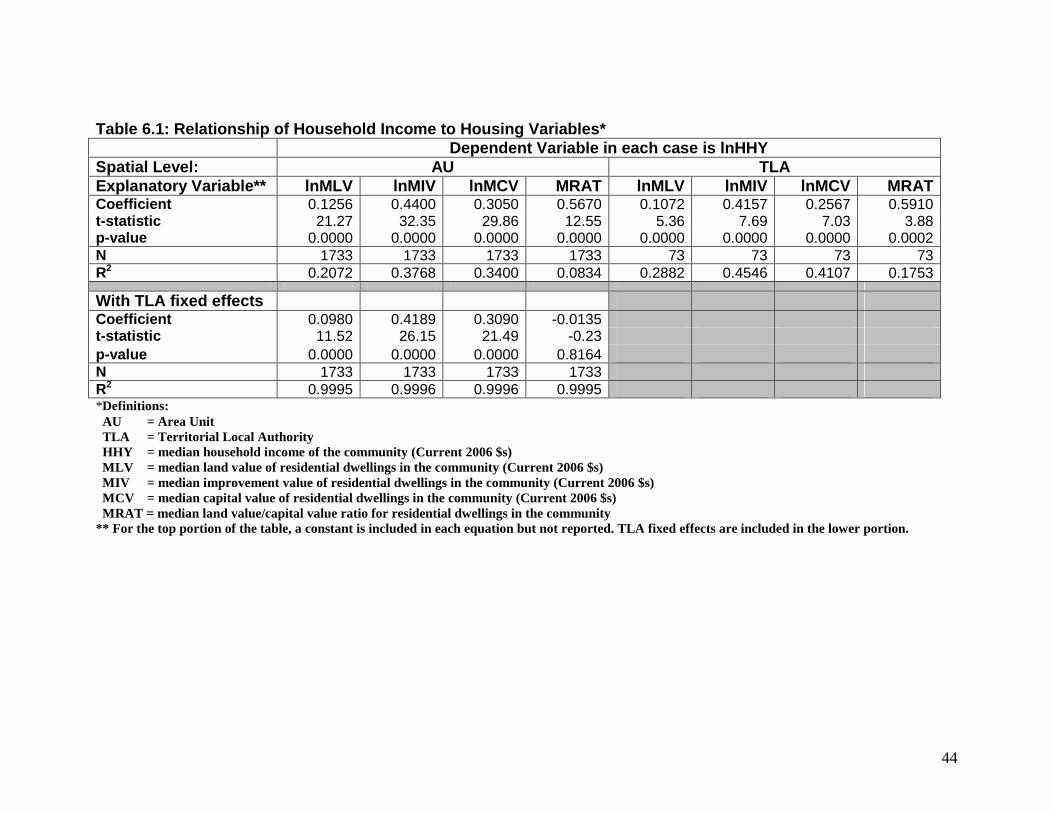
44

Table 6.1: Relationship of Household Income to Hous ing Variables* Dependent Variable in each case is lnHHY Spatial Level: AU TLA Explanatory Variable** lnMLV lnMIV lnMCV MRAT lnMLV lnMIV lnMCV MRAT Coefficient 0.1256 0.4400 0.3050 0.5670 0.1072 0.4157 0.2567 0.5910 t-statistic 21.27 32.35 29.86 12.55 5.36 7.69 7.03 3.88 p-value 0.0000 0.0000 0.0000 0.0000 0.0000 0.0000 0.0000 0.0002 N 1733 1733 1733 1733 73 73 73 73 R2 0.2072 0.3768 0.3400 0.0834 0.2882 0.4546 0.4107 0.1753

With TLA fixed effects Coefficient 0.0980 0.4189 0.3090 -0.0135 t-statistic 11.52 26.15 21.49 -0.23 p-value 0.0000 0.0000 0.0000 0.8164 N 1733 1733 1733 1733 R2 0.9995 0.9996 0.9996 0.9995 *Definitions: AU = Area Unit TLA = Territorial Local Authority HHY = median household income of the community (Current 2006 $s) MLV = median land value of residential dwellings in the community (Current 2006 $s) MIV = median improvement value of residential dwellings in the community (Current 2006 $s) MCV = median capital value of residential dwellings in the community (Current 2006 $s) MRAT = median land value/capital value ratio for residential dwellings in the community ** For the top portion of the table, a constant is included in each equation but not reported. TLA fixed effects are included in the lower portion.

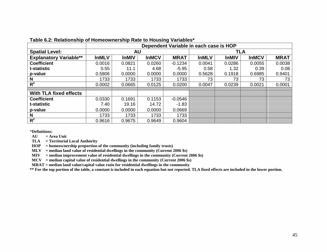
45

Table 6.2: Relationship of Homeownership Rate to Ho using Variables* Dependent Variable in each case is HOP Spatial Level: AU TLA Explanatory Variable** lnMLV lnMIV lnMCV MRAT lnMLV lnMIV lnMCV MRAT Coefficient 0.0016 0.0821 0.0260 -0.1234 0.0041 0.0286 0.0055 0.0038 t-statistic 0.55 11.1 4.68 -5.95 0.58 1.32 0.39 0.08 p-value 0.5806 0.0000 0.0000 0.0000 0.5628 0.1918 0.6985 0.9401 N 1733 1733 1733 1733 73 73 73 73 R2 0.0002 0.0665 0.0125 0.0200 0.0047 0.0239 0.0021 0.0001

With TLA fixed effects Coefficient 0.0330 0.1691 0.1153 -0.0546 t-statistic 7.40 19.16 14.72 -1.83 p-value 0.0000 0.0000 0.0000 0.0669 N 1733 1733 1733 1733 R2 0.9616 0.9675 0.9649 0.9604 *Definitions: AU = Area Unit TLA = Territorial Local Authority HOP = homeownership proportion of the community (including family trusts) MLV = median land value of residential dwellings in the community (Current 2006 $s) MIV = median improvement value of residential dwellings in the community (Current 2006 $s) MCV = median capital value of residential dwellings in the community (Current 2006 $s) MRAT = median land value/capital value ratio for residential dwellings in the community ** For the top portion of the table, a constant is included in each equation but not reported. TLA fixed effects are included in the lower portion.

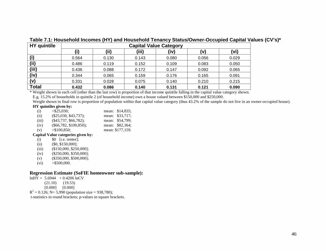
46

Table 7.1: Household Incomes (HY) and Household Ten ancy Status/Owner-Occupied Capital Values (CV’s)* Capital Value Category HY quintile

(i) (ii) (iii) (iv) (v) (vi) (i) 0.564 0.130 0.143 0.080 0.056 0.029 (ii) 0.486 0.119 0.152 0.109 0.083 0.050 (iii) 0.436 0.088 0.172 0.147 0.092 0.065 (iv) 0.344 0.065 0.159 0.176 0.165 0.091 (v) 0.331 0.028 0.075 0.140 0.210 0.215 Total 0.432 0.086 0.140 0.131 0.121 0.090 * Weight shown in each cell (other than the last row) is proportion of that income quintile falling in the capital value category shown. E.g. 15.2% of households in quintile 2 (of household income) own a house valued between $150,000 and $250,000. Weight shown in final row is proportion of population within that capital value category (thus 43.2% of the sample do not live in an owner-occupied house). HY quintiles given by:

(i) <$25,030; mean: $14,835; (ii) ($25,030, $43,737); mean: $33,717; (iii) ($43,737, $66,782); mean: $54,799; (iv) ($66,782, $100,850); mean: $82,364; (v) >$100,850; mean: $177,159.

Capital Value categories given by: (i) $0 [i.e. renter]; (ii) ($0, $150,000]; (iii) ($150,000, $250,000]; (iv) ($250,000, $350,000]; (v) ($350,000, $500,000]; (vi) >$500,000.

Regression Estimate (SoFIE homeowner sub-sample): lnHY = 5.6944 + 0.4206 lnCV

(21.10) (19.53) [0.000] [0.000]

R2 = 0.126; N= 5,990 (population size = 938,780); t-statistics in round brackets; p-values in square brackets.

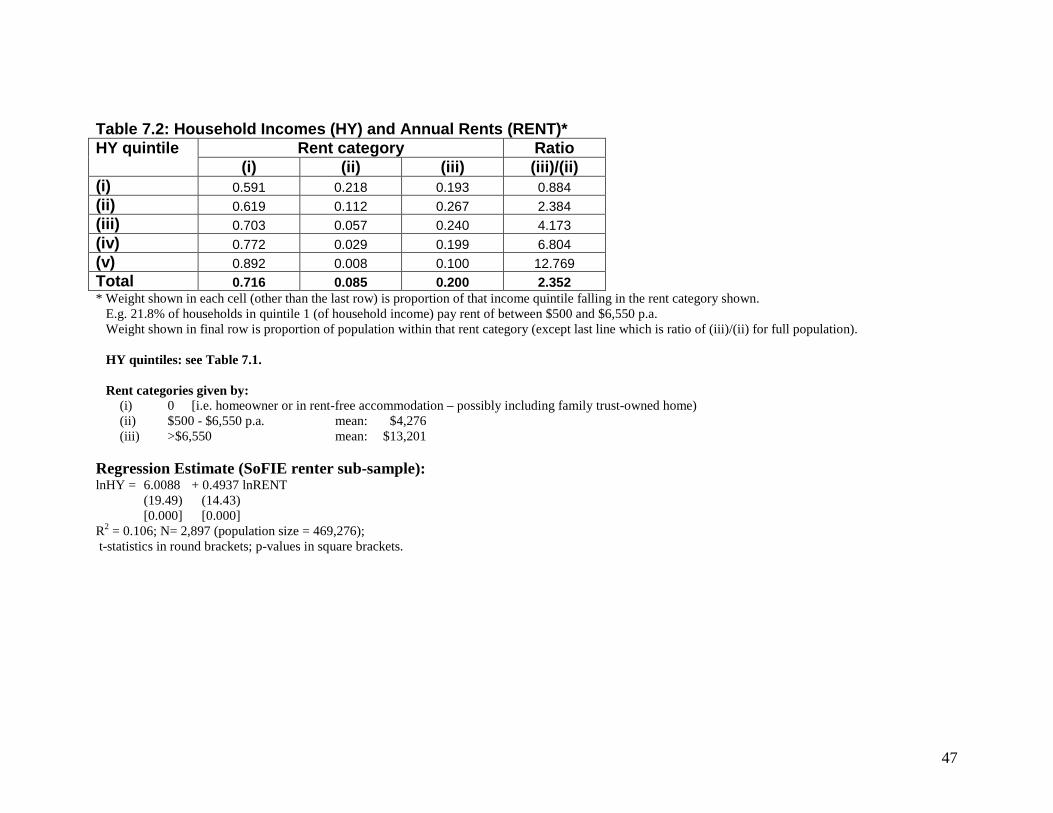
47

Table 7.2: Household Incomes (HY) and Annual Rents (RENT)* Rent category Ratio HY quintile

(i) (ii) (iii) (iii)/(ii) (i) 0.591 0.218 0.193 0.884 (ii) 0.619 0.112 0.267 2.384 (iii) 0.703 0.057 0.240 4.173 (iv) 0.772 0.029 0.199 6.804 (v) 0.892 0.008 0.100 12.769 Total 0.716 0.085 0.200 2.352 * Weight shown in each cell (other than the last row) is proportion of that income quintile falling in the rent category shown. E.g. 21.8% of households in quintile 1 (of household income) pay rent of between $500 and $6,550 p.a. Weight shown in final row is proportion of population within that rent category (except last line which is ratio of (iii)/(ii) for full population). HY quintiles: see Table 7.1. Rent categories given by:

(i) 0 [i.e. homeowner or in rent-free accommodation – possibly including family trust-owned home) (ii) $500 - $6,550 p.a. mean: $4,276 (iii) >$6,550 mean: $13,201

Regression Estimate (SoFIE renter sub-sample): lnHY = 6.0088 + 0.4937 lnRENT

(19.49) (14.43) [0.000] [0.000]

R2 = 0.106; N= 2,897 (population size = 469,276); t-statistics in round brackets; p-values in square brackets.

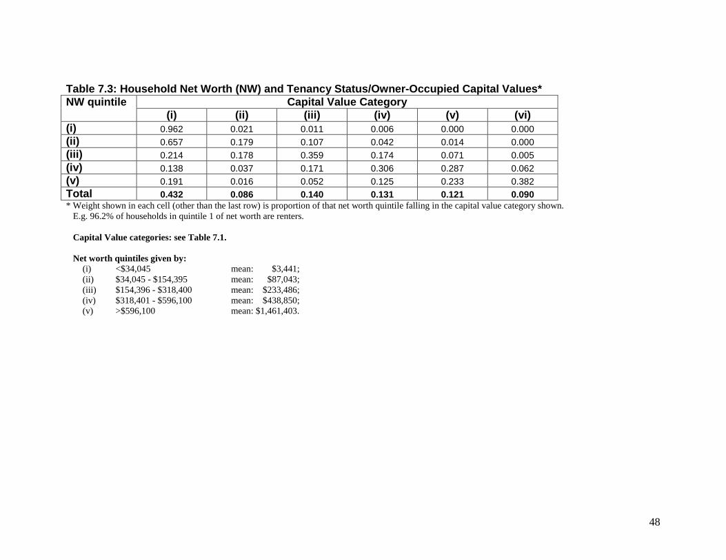
48

Table 7.3: Household Net Worth (NW) and Tenancy Sta tus/Owner-Occupied Capital Values* Capital Value Category NW quintile

(i) (ii) (iii) (iv) (v) (vi) (i) 0.962 0.021 0.011 0.006 0.000 0.000 (ii) 0.657 0.179 0.107 0.042 0.014 0.000 (iii) 0.214 0.178 0.359 0.174 0.071 0.005 (iv) 0.138 0.037 0.171 0.306 0.287 0.062 (v) 0.191 0.016 0.052 0.125 0.233 0.382 Total 0.432 0.086 0.140 0.131 0.121 0.090 * Weight shown in each cell (other than the last row) is proportion of that net worth quintile falling in the capital value category shown. E.g. 96.2% of households in quintile 1 of net worth are renters. Capital Value categories: see Table 7.1. Net worth quintiles given by:

(i) <$34,045 mean: $3,441; (ii) $34,045 - $154,395 mean: $87,043; (iii) $154,396 - $318,400 mean: $233,486; (iv) $318,401 - $596,100 mean: $438,850; (v) >$596,100 mean: $1,461,403.

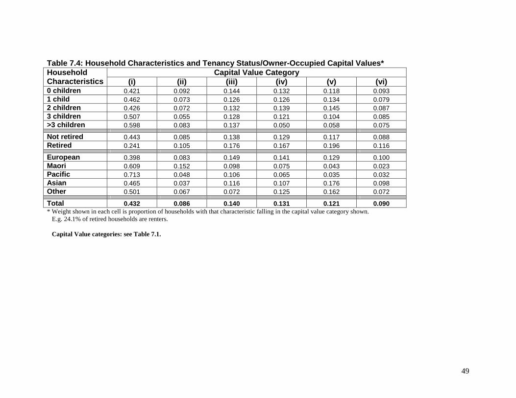
49

Table 7.4: Household Characteristics and Tenancy St atus/Owner-Occupied Capital Values* Capital Value Category Household

Characteristics (i) (ii) (iii) (iv) (v) (vi) 0 children 0.421 0.092 0.144 0.132 0.118 0.093 1 child 0.462 0.073 0.126 0.126 0.134 0.079 2 children 0.426 0.072 0.132 0.139 0.145 0.087 3 children 0.507 0.055 0.128 0.121 0.104 0.085 >3 children 0.598 0.083 0.137 0.050 0.058 0.075

Not retired 0.443 0.085 0.138 0.129 0.117 0.088 Retired 0.241 0.105 0.176 0.167 0.196 0.116

European 0.398 0.083 0.149 0.141 0.129 0.100 Maori 0.609 0.152 0.098 0.075 0.043 0.023 Pacific 0.713 0.048 0.106 0.065 0.035 0.032 Asian 0.465 0.037 0.116 0.107 0.176 0.098 Other 0.501 0.067 0.072 0.125 0.162 0.072

Total 0.432 0.086 0.140 0.131 0.121 0.090 * Weight shown in each cell is proportion of households with that characteristic falling in the capital value category shown. E.g. 24.1% of retired households are renters. Capital Value categories: see Table 7.1.