NBER WORKING PAPER SERIES

DISTRIBUTIONAL IMPACTS OF THESELF-SUFFICIENCY PROJECT

Marianne P. BitlerJonah B. GelbachHilary W. Hoynes

Working Paper 11626http://www.nber.org/papers/w11626

NATIONAL BUREAU OF ECONOMIC RESEARCH1050 Massachusetts Avenue

Cambridge, MA 02138September 2005

Correspondence to Hoynes at UC Davis, Department of Economics, 1152 Social Sciences and HumanitiesBuilding, One Shields Avenue, Davis, CA 95616-8578, phone (530) 752-3226, fax (530) 752-9382, orhwhoynes@ucdavis.edu; Gelbach at gelbach@glue.umd.edu; or Bitler at bitler@ppic.org. We are gratefulto Human Resources Development Canada for funding this experiment and to SDRC for research supportand for making the SSP data available. We thank Douglas Tattrie and Kevin Milligan for helpfulconversations and Peter Huckfeldt for research assistance. All conclusions in this paper are solely theresponsibility of the authors, and do not represent the opinions or conclusions of HDRC, SDRC, theCanadian government, the sponsors of the Self-Sufficiency Project, or any other institution. The viewsexpressed herein are those of the author(s) and do not necessarily reflect the views of the National Bureauof Economic Research.

©2005 by Marianne P. Bitler, Jonah B. Gelbach and Hilary W. Hoynes. All rights reserved. Short sectionsof text, not to exceed two paragraphs, may be quoted without explicit permission provided that full credit,including © notice, is given to the source.

Distributional Impacts of the Self-Sufficiency ProjectMarianne P. Bitler, Jonah B. Gelbach and Hilary W. HoynesNBER Working Paper No. 11626September 2005JEL No. J2, I38, H53

ABSTRACT

A large literature has been concerned with the impacts of recent welfare reforms on income,earnings, transfers, and labor-force attachment. While one strand of this literature relies onobservational studies conducted with large survey-sample data sets, a second makes use of datagenerated by experimental evaluations of changes to means-tested programs. Much of the overallliterature has focused on mean impacts. In this paper, we use random-assignment experimental datafrom Canada's Self-Sufficiency Project (SSP) to look at impacts of this unique reform on thedistributions of income, earnings, and transfers. SSP offered members of the treatment group agenerous subsidy for working full time. Quantile treatment effect (QTE) estimates show there wasconsiderable heterogeneity in the impacts of SSP on the distributions of earnings, transfers, and totalincome; heterogeneity that would be missed by looking only at average treatment effects. Moreover,these heterogeneous impacts are consistent with the predictions of labor supply theory. During theperiod when the subsidy is available, the SSP impact on the earnings distribution is zero for thebottom half of the distribution. The SSP earnings distribution is higher for much of the upper thirdof the distribution except at the very top, where the earnings distribution is the same under eitherprogram or possibly lower under SSP. Further, during the period when SSP receipt was possible, theimpacts on the distributions of transfer payments (IA plus the subsidy) and total income (earningsplus transfers) are also different at different points of the distribution. In particular, positive impactson the transfer distribution are concentrated at the lower end of the transfer distribution whilepositive impacts on the income distribution are concentrated in the upper end of the incomedistribution. Impacts of SSP on these distributions were essentially zero after the subsidy was nolonger available.

Marianne BitlerPublic Policy Institute of California500 Washington StreetSan Francisco, CA 94111bitler@ppic.org

Jonah GelbachDepartment of EconomicsUniversity of MarylandCollege Park, MD 20742gelbach@glue.umd.edu

Hilary HoynesDepartment of EconomicsUniversity of California, Davis1152 Social Sciences and HumanitiesBuildingOne Shields AvenueDavis, CA 95616-8578and NBERhwhoynes@ucdavis.edu

1

I. Introduction

As we move into the 21st century, government assistance for poor families has undergone

major reform across Europe, Canada and the United States. In some cases, changes have taken

place within traditional government welfare programs (e.g., the SSP demonstration in Canada

and welfare reform in the United States) to reduce the negative work incentives embodied in

programs that taxed away welfare benefits at a high rate with each extra dollar in earnings. In

other cases, new programs have been added or expanded providing in-work subsidies for low

income workers and families. Prominent examples of these policies are the United States’ Earned

Income Tax Credit and the United Kingdom’s Working Family Tax Credit. Further, a recent

report identifies nine OECD countries (including the United States and United Kingdom) that

offer in-work subsidies (Owens 2005). A common feature of these program changes is

expanding the financial gains to working. In so doing, the goal of the policy changes is to ‘make

work pay’ and increase self sufficiency.

In this dynamic policy environment, a large literature has developed.1 A common feature

of this literature is the focus on the mean impacts of the policy of interest. In this paper, we make

an important contribution to the literature by using a simple nonparametric estimator — quantile

treatment effects, or QTEs — to estimate the impact of an important policy change on the

distribution of earnings and income outcomes.

Many governments have conducted randomized experiments to assess the impacts of

generous financial incentives for work on welfare and employment among cash assistance

recipients. One such experiment, the Self-Sufficiency Project (SSP), has received an enormous

1 For example, in the United States, Grogger & Karoly (2005) provide a summary of welfare reform and Hotz & Scholz (2003) and Eissa & Hoynes (Forthcoming) provide reviews of the Earned Income Tax Credit. Blundell & Hoynes (2004) compare the United States’ and United Kingdom’s in-work policies, and evaluations of the Working Family Tax Credit appear in Blundell et al., (2005), Brewer et al., (2005), Francesconi & van der Klauw (2004), Gregg & Harkness (2003), and Leigh (2004). Bargain & Orsini (2004) and Smith et al., (2003) use cross-country data to evaluate European reforms.

2

amount of attention due to its ability to increase earnings and income. For example, findings

about SSP were cited in numerous U.K. government documents as inspiration for reforms

instituted by the Labour government in the late 1990s. SSP was sponsored by Human Resources

Development Canada and conducted by the Social Research Demonstration Corporation. SSP

was designed to test the impact of a generous earnings subsidy for full-time work on long-term

welfare participants.

Between 1992 and 1995, SSP randomly assigned a group of single-parent recipients and

applicants for income assistance (IA) in two provinces, New Brunswick and British Columbia, to

treatment and control groups. Control group members faced the rules of IA in their home

province. Treatment group members who had been on IA for 12 of the previous 13 months were

eligible for a generous earnings supplement if they could find full time work (at least 30 hours a

week) at or above the minimum wage within a year. The earnings supplement was one-half the

difference between their earnings and a benchmark earnings level ($30,000 in New Brunswick

and $37,000 in British Columbia) and was available for 36 months. Persons receiving the

supplement had to forego their IA payments, although if they gave up the supplement, they could

receive IA if they were otherwise eligible.

Several final reports (Michalopoulos et al., 2002 and Ford et al., 2003), and a large

number of research papers (e.g., Blank et al. , 2000; Card & Hyslop, 2004; Card et al., 2001;

Connolly & Gottschalk, 2003; Foley, 2004; Foley & Schwartz 2002; Harknett & Gennetian,

2003; Kamionka & Lacroix, 2003; Lise et al., 2005; Michalopoulos et al., 2005; Zabel et al.,

2004) have looked at the overall impacts of the SSP experiment on income, earnings, labor force

attachment, unemployment durations, wages, wage growth, job choice, and marriage. These

papers find that the program increased employment, earnings, and income considerably during

3

the years when the supplement was available, while having little or no impacts after the

supplement was no longer available.

Existing literature focuses on SSP’s mean impacts, in the full sample and in demographic

subgroups. Mean impacts, however, may conceal heterogeneous impacts across the distribution

of earnings and income. For example, SSP generates an increase in total income and net wages at

30 hours of work and above. The income gains are substantial — most families had after-tax

annual incomes $3,000–$7,000 higher with SSP than they would have had if they had worked

the same number of hours under IA (Michalopoulos et al., 2002). Static labor supply theory

predicts that this increase in nonlabor income would lead some recipients to increase work and

leave IA, thereby increasing earnings and income. On the other hand, workers who would work

full-time under IA-only assignment receive a windfall payment under SSP, which could lead to

much smaller (and possibly negative) earnings effects based on standard labor supply analysis.

In this paper, we move beyond mean impacts and examine the impacts of SSP on the

distribution of earnings, transfers, and income using QTE estimation.2 We estimate the QTEs

very simply as the difference in outcomes at various quantiles of the treatment (SSP) and control

(IA-only) group distributions. Thus, QTEs tell us how the earnings distribution changes when we

assign SSP treatment randomly. The QTE is a simple nonparametric estimator that requires only

that the treatment is randomly assigned. As we discuss in more detail below, QTEs identify only

the impact of treatment on the distribution; this impact is distinct from, and in general not equal

to, the distribution of treatment effects (as well as other interesting estimates, such as the

treatment effect on people whose control-group outcome would have been the median, etc.).

2 A host of authors have used QTEs (e.g., Heckman, Smith, & Clements, 1997; Firpo, 2004). Friedlander & Robins (1997) estimate QTEs to evaluate the impact of employment training programs in early welfare-reform experiments. Bitler, Gelbach, & Hoynes (Forthcoming) examine the impact of a welfare-reform experiment in Connecticut in the mid-1990s on AFDC and Food Stamp payments, earnings, and total income.

4

In this paper, we contribute to the literature on the impacts of financial incentives on

labor supply and to the existing experimental literature including our own earlier work (Bitler et

al., Forthcoming) in three ways. First, SSP is an important policy that has received a great deal of

attention in the international policy arena, influencing adoption of new policies and experiments

in Europe. The minimum work requirement and relatively generous benefits make the policy

unique and have important implications for the impacts of the policy. For example, SSP moved

long term recipients into the labor force much more quickly than they would have under Income

Assistance while nearly paying for itself, costing a scant $4000 more per recipient over a 5-year

period than Income Assistance (Michalopoulos et al., 2002). Our distributional analysis adds to

our understanding of SSP in a fundamental way.3 Second, the SSP experiment is unusual in that

it provides data on wages and hours thereby allowing for a much richer analysis of the labor

supply implications relative to our earlier work (Bitler et al., Forthcoming). Finally, to our

knowledge we are the first to explore empirically the validity of the rank preservation

assumption — that is the assumption that one’s spot in the distribution of income (or earnings or

transfers) is invariant to program assignment. If rank preservation holds, then the QTEs we

present are identical to the distribution of treatment effects, and can be used to assess how

individuals at various points in a distribution are affected by the program. Understanding the

extent to which people move across the distribution is important for interpretation of the results.

Our results show that the SSP program indeed had heterogeneous impacts across the

earnings, transfer, and income distributions. During the period when the subsidy is available, the

impact of SSP on the earnings distribution is zero for the bottom half of the distribution. The SSP

3 Michalopoulos et al. (2002, 2005) examine the impact of SSP on poverty rates and on ranges of hours worked and hourly wage rates. While this provides some insight into the distributional analysis, our analysis is more comprehensive in that it also analyzes impacts on earnings, income, and transfers. We also examine the full 54 month follow-up period rather than analyzing data from a few months, making our results more representative of the longer run impacts of SSP. Finally, their analyses focus on wages among the employed. By contrast, we consider the distribution of wages for everyone, which takes account of the changes in employment rates and allows for more clean interpretation of the results.

5

earnings distribution is higher for much of the upper third of the distribution except at the very

top, where the earnings distribution is the same under either program or possibly lower under

SSP. Further, during the SSP receipt period, the impacts on the distributions of transfer payments

(IA plus the subsidy) and total income (earnings plus transfers) are also different at different

points of these distributions. Positive impacts on the transfer distribution are concentrated at the

lower end of the transfer distribution. By contrast, positive impacts on the income distribution

are concentrated at the upper end of the income distribution, suggesting that within this group of

long term welfare recipients, the program benefited the top of the distribution more than the

bottom.4 Impacts of SSP on these distributions were essentially zero or negative after the subsidy

was no longer available.5

We argue that these findings are consistent with labor supply theory — workers respond

to the financial incentives by changing their hours worked and, in some cases, reducing the

reservation wages at which they will just be willing to take a job. We can explore these pathways

more convincingly in this setting because we have data on wages and hours.

Finally, our tests of rank preservation suggest that there is some evidence of rank reversal

(along observable dimensions).

The remainder of this paper is organized as follows. In Section II, we discuss the SSP

experiment and the financial incentives in IA and SSP. In Section III, we use theoretical

predictions about labor supply to discuss the expected effects of SSP on labor supply, welfare

receipt, and income. Section IV discusses the empirical methods and Section V describes our

data and presents descriptive statistics and reviews the mean treatment effects. Our main QTE

4 As we discuss below, a person whose transfer payments are at the bottom of the transfers distribution will not necessarily have income at the bottom of the income distribution (in fact, we would typically expect the opposite to be true). 5 Note that persons assigned to the supplement group could always obtain Income Assistance (indefinitely) if they were income eligible and not receiving the supplement. This suggests that we might not see large “losers” in the supplement group as IA provided a safety net. This is in contrast to the findings for welfare recipients facing time limits in the post-TANF policy setting in the U.S. (Bitler et al., Forthcoming).

6

results are presented in Section VI. We explore the validity of the rank preservation assumption

in Section VII and we conclude in Section VIII.

II. SSP, Income Assistance, and the SSP Experiment

The SSP experiment randomly assigned welfare recipients to a treatment group — who

could obtain SSP — or a control group — who had access only to the existing Income

Assistance (IA) program. In this paper, we use data from the SSP Recipient sample which

consists of about 6,000 single parents aged 19 or older in British Columbia and New Brunswick

who had been on IA for at least 12 month of the last 13 months.6 Random assignment began in

November 1992 and ended in March 1995. We begin by describing the financial incentives in IA

and SSP. This will provide background for discussing the expected impact of SSP, which we

cover in the next section.

Income assistance was (at the time of the SSP experiment) Canada’s universal cash safety

net program.7 The program covers all demographic groups and, in particular, is available to

families without children as well as those with children. Benefits are means tested using income

and asset tests, and eligibility thresholds and benefit levels vary by province and family size. The

IA benefit structure is typical of means-tested transfer programs and is characterized by a

guaranteed income (the benefit received if the family has no other income) and a benefit

reduction rate or phase-out rate which dictates how the benefit is reduced as earned income

increases. The IA program is quite generous — in 1992 the annual guarantee for a single-parent

family with one child was $13,752 in British Columbia and $8,964 in New Brunswick. As is

6 We exclude the SSP Plus sample (293 observations) from our analysis because we wish to focus on the impact of the financial incentives in SSP alone, which may be confounded with the effects of the employment services also offered in SSP Plus (e.g., Michalopoulos et al., 2002). We also ignore the SSP Applicant sample, made up of new applicants at the time of random assignment, who had to stay on welfare for 12 months to become eligible for the supplement. 7 Information about IA is drawn from Barrett, Doiron, Green, & Riddell, 1996; Michalopoulos et al., 2002; and Ford et al., 2003.

7

common with welfare programs, the long-run benefit reduction rate was very high, leading to

large work disincentives. Specifically, in 1992, IA recipients in New Brunswick faced a 100 per

cent benefit reduction rate for every dollar earned over $200 per month. In British Columbia, the

disregard was also $200 a month while the benefit reduction rate was 75 per cent for 12 out of

each 36 months and 100 per cent for the other 24 months out of 36.8

The SSP earnings supplement is a negative-income-tax style transfer payment with a

minimum hours of work restriction. In particular, to be eligible for a supplement payment, one

had to work full-time (an average of at least 30 hours a week over a four-week period) at one or

more jobs paying at least the minimum wage. During the experimental period, the minimum

wage in British Columbia started at $5.50 an hour and increased to $7.15 in 1998 and the

minimum wage in New Brunswick ranged from $5.00 an hour at the beginning of the period to

$5.50 in 1996. Supplement recipients could not receive IA at the same time as they received the

supplement, but supplement recipients could return to IA at any time (if income and otherwise

eligible) and could also rejoin the supplement group if they met the hours and wage restrictions

while the supplement was available. The ongoing IA eligibility suggests that members of the

treatment group had a safety net if they could not find work. Lastly, to target the program to

long-term welfare recipients, eligibility for the supplement required having been on IA for 12 of

the past 13 months.

The supplement is equal to one-half the difference between recipient earnings and a

benchmark earnings amount (unearned income was not considered when calculating the

8 In September 1995, New Brunswick increased the earnings disregard for the first 12 months on aid to a flat amount of $200 or a 35 per cent disregard (whichever was larger) for 6 months and then $200 or 30 per cent for 6 months. In April 1996, the flat disregard of $200 per month was eliminated in British Columbia. In 1996, federal funding for IA was reduced and converted to a block grant. Some provinces — including British Columbia — responded by reducing benefit levels or tightening eligibility requirements. In 1996, British Columbia established sanctions for anyone who quit a job without just cause, barring IA eligibility for 6 months. Later in 1996, British Columbia made its eligibility determination process more stringent. In addition, in 1996, British Columbia created a “Family Bonus” of $103 per child (for all low-income families with children), and reduced IA benefits by the same amount. New Brunswick introduced a similar Child Tax Benefit, but it was much smaller (up to $250 per child per year).

8

supplement payment). At the beginning of the experiment, the benchmark was $37,000 in British

Columbia and $30,000 in New Brunswick.9 This benefit structure is equivalent to a guaranteed

income which begins at an earnings level of the minimum hours point times the minimum wage

and is then phased out using a 50 per cent benefit reduction rate with a breakeven point equal to

the earnings benchmark. SSP represented a substantial increase in the financial incentives for

work compared to the incentives in the IA program.

The SSP experiment gave recipients 12 months to establish full-time work and take up

the supplement. If recipients did not take-up the supplement within 12 months, they were

ineligible to obtain it at all. Employers were not informed of supplement receipt by the provinces

and program participants had to mail in pay-stubs to obtain supplement payments. Takers could

receive the supplement for up to three years from the time when it started. Importantly, they

could not bank the supplement for later use.

III. Expected Impacts of the SSP Supplement

To motivate our interest in measuring the impact of SSP on the distribution of earnings

and income, it is useful to outline the incentives facing welfare recipients in the SSP and IA

groups. We should note that this section describes incentives for individuals and does not,

therefore, map directly into our QTE measures of impacts of SSP on the distributions.

We examine potentially heterogeneous impacts of SSP on earnings, transfers, and income

through two channels. We begin with a static labor supply model where women can freely

choose hours of work at the given offered wage and offered wages are constant. (Note that we

use women to refer to persons in the experiment for expediency: 96 per cent of those in our final

9 The earnings benchmarks were adjusted each year for inflation. For more on the annual earnings benchmarks see Michalopoulos et al., (2002).

9

sample were females.) We then discuss the expected impacts on wages using the dynamic search

model in Card & Hyslop (2004).

To guide the discussion, Figure 1 presents a stylized budget constraint for IA and SSP.

The figure plots hours of work on the horizontal axis and income (from IA/SSP and earnings) on

the vertical axis. The IA portion of the budget set goes from hours of 0 to H1 (the IA breakeven

point): if the woman does not work, she gets the maximum IA benefit. Then, for each additional

dollar in earnings, the IA benefit is reduced by one dollar resulting in a slope of 0 for the IA

budget constraint.10 If assigned to the SSP group, a woman is eligible for SSP if she works

beyond the hours restriction labeled H* in Figure 1. At H*, income increases by the SSP

supplement, which is equal to one-half of the difference between earnings and the benchmark

earnings amount, labeled E2. Therefore, the slope of the SSP portion of the budget set is one-half

of the hourly wage w. In this stylized figure, the minimum hours restriction is set below the IA

breakeven point (H*< H1). This may not be the case for all families — those with higher wages

may have H*>H1.11

We begin by considering the static labor supply model with constant wages. The idea is

to compare the labor supply incentives for someone facing IA-only to the counterfactual state of

the world in which she is assigned to SSP. Consider the case in which a woman would choose

not to work when assigned to IA only. Depending on her preferences, assignment to SSP may

lead her to enter the labor market and work hours H, where H2>H>H*. Alternatively, she may

continue to work zero hours and receive the maximum IA payment. The same qualitative

predictions hold for a woman who, when assigned to IA only, chooses to receive IA and work

below the hours restriction H*.

10 This stylized budget constraint captures neither the flat earnings disregards in IA nor the lower than 100 per cent tax rate that held in some periods. These features do not alter the qualitative statements that we make here. 11 In addition, the stylized budget constraint shows that the SSP payment at H* is larger than the IA guarantee which is true for (at least) minimum-wage workers. In general, the maximum SSP payment is inversely related to the wage.

10

We next consider a woman who, when assigned to the IA-only group, eventually leaves

IA and works at hours levels above H1. In the counterfactual assignment to SSP, she finds

herself in the “windfall” group where she is eligible for SSP and gains income without any

change in behavior. Ashenfelter (1983) referred to this as a “mechanical” induced eligibility

effect. This effect leads to an ambiguous impact on hours worked depending on whether or not

the 30 hour per week requirement (H*) is above or below the IA breakeven point (H1). SSP

leads to an increase in nonlabor income and a decrease in the net wage, both of which lead to a

decrease in desired hours. However, if H* is above H1 (not as drawn in Figure 1), it is possible

that to obtain the SSP supplement, the woman may need to increase her hours. Importantly, for

the vast bulk of women in this group, we do not expect the increase in desired hours that is

experienced by the nonworking group discussed above. We instead expect hours to decrease for

the bulk of the women. Lastly, consider a woman who might have eventually left IA and worked

at a high level, say H>H2 (yielding income too high for SSP eligibility). She may be induced to

decrease her hours, compared to her counterfactual choice under IA only, to become eligible for

SSP. Ashenfelter (1983) refers to this group as having a “behavioral” induced eligibility effect.12

Now consider the impact of SSP in the context of a dynamic search model. Card &

Hyslop (2004) outline such a model and find that SSP should induce women to search more

intensely; they might also accept jobs with lower reservation wages than they would under

counterfactual IA in order to become eligible for the supplement. Further, Card & Hyslop (2004)

find that a woman’s reservation wage decreases as she approaches the one-year time limit for

establishing eligibility for SSP. These results need not imply that wages will decrease throughout

the distribution, however. SSP requires work at the minimum wage or higher — so lower-skill

12 During months 1–54, only 1.8 per cent of the British Columbia control sample, and 1.8 per cent of the New Brunswick control sample had monthly earnings that would make them ineligible for SSP (under random-assignment eligibility levels), suggesting that a small share of the overall distribution might face such a behavioral induced eligibility effect.

11

women are unable to reduce their reservation wage below the minimum. Consequently, the

reduction in wages will be concentrated at upper end of the wage distribution.

In sum, the expected impacts on earnings are heterogeneous and may be negative, zero,

or positive. The static labor supply model predicts no change in earnings at the bottom of the

distribution, an increase in earnings in the middle of the distribution, with little change (and

possibly a reduction) in earning at the top of the distribution. There might also be reductions

somewhat below the top of the earnings distribution, if income effects dominate for those women

who would not receive IA when assigned to the control group but would be income-eligible for

SSP holding constant their behavior. Further, the dynamic search model implies that earnings

may decrease due to a reduction in reservation wages, and this is also likely to be concentrated at

the top of the earnings distribution (if high-wage individuals are also high-earnings individuals).

Therefore we can assess the contribution of these two channels — hours and wages — to the

changes in earnings.

This discussion can also be extended to consider impacts of SSP on transfer income (IA

plus SSP if eligible) and total income. The increase in transfers is likely to be concentrated at the

bottom of the transfer distribution (among those with lower welfare use) with small or no gains

at the top of the transfer distribution. The impact on the distribution of income depends on the

relative change in earnings and transfers but is likely to be zero at the bottom of the distribution

(where women stay on IA) and higher at the top of the distribution (where high-skill women get

the windfall of SSP).

IV. QTE Methodology

The evaluation reports present mean differences between treatments and controls for

employment, income, wages, transfers, and children’s outcomes at each of the follow-up surveys

12

(e.g., Michalopoulos et al., 2002). Given random assignment to the program, these mean

differences are reliable estimates of the true mean impact of the program. The above discussion

of the impacts of SSP suggest that mean impacts may conceal heterogeneous impacts across the

distribution. Here we outline the quantile treatment effect (QTE) estimator that we use to

examine the impact of SSP on the entire distribution of earnings (and transfer payments and total

income).

The QTE for quantile q may be estimated very simply as the difference across treatment

status in the quantiles of outcomes for the two groups (treatments and controls). To understand

QTE, imagine that we take a large group of people — say, N=N1+N0 in number — and

randomly assign N1 of them to SSP and N0 of them to IA. For concreteness, suppose we are

interested in the effect of SSP on the 25th quantile of the earnings distribution. The 25th quantile

of the SSP group's earnings distribution is the smallest level of earnings such that at least 25 per

cent of SSP-assigned people have earnings below that level. Similarly, the 25th quantile of the IA

group's earnings distribution is the smallest level of earnings such that at least 25 per cent of IA-

assigned people have earnings below that level. The QTE at the 25th quantile is the difference in

these two earnings levels. Thus, QTEs tell us how the earnings distribution changes when we

assign SSP treatment randomly. Other quantile treatment effects are estimated analogously, and

we evaluate the distributions at 99 centiles.

One important methodological distinction is between quantile treatment effects and

quantiles or other features of the treatment effect distribution. To understand the distinction, it

will be helpful to briefly introduce a model of causal effects. Let Ti=1 if observation i receives

the treatment, and 0 otherwise. Let Yi(t) be i's counterfactual value of the outcome Y if i has Ti=t.

The fundamental evaluation problem is that for any i, at most one element of the pair (Yi(0),

13

Yi(1)) can ever be observed: we cannot observe someone who is simultaneously treated and not

treated.

Evaluation methodology focuses on inferences concerning various features of the joint

distribution of (Y(0),Y(1)). In particular, the marginal distributions F0(y) and F1(y) are always

identified, where Ft(y)= Pr[Yi(t)< y] for a randomly drawn i. There is an enormous literature

concerning this model and the assumptions under which it is useful. See, for example, papers by

Heckman et al., (1997) or Imbens & Angrist (1994) for further details.

Quantile treatment effects are features of the marginal distributions F0(y) and F1(y). For

treatment assignment t, the qth quantile of distribution Ft is defined as yq(t) ≡ inf{y:Ft(y)≥q}. The

quantile treatment effect for quantile q is then simply the difference in the two qth quantiles of

the two distributions:

Δq = yq(1) - yq(0).

Our above example concerning the QTE for the 25th quantile involves setting q=0. 25. Thus the

estimated quantile treatment effect is the simple difference between quantiles of the distribution

for the treatment and control groups

By contrast, for observation i, the treatment effect is δi= Yi(1)-Yi(0), and the cumulative

distribution of treatment effects may be written as G(d)= Pr[δi ≤ d] for randomly chosen i. Thus,

unlike quantile treatment effects, quantiles of the distribution of treatment effects cannot be

written as features of the marginal distributions. Rather, they require more detailed knowledge of

the joint distribution (e.g., further assumptions about it).

Under some conditions, the distribution of treatment effects is recoverable from the

quantile treatment effects. For example, if the treatment effect is equal for all observations then

the distribution G is degenerate and is fully identified by the mean impact. However, the above

discussion of labor supply impacts suggests that such a homogeneity restriction is not valid here.

14

Second, if people’s ranks in the distributions are the same regardless of whether they are

assigned to treatment or control group (e.g., there is rank preservation across treatment status),

then the QTE at quantile q tells us the treatment effect for the person located at quantile q in the

given distribution. Under rank preservation, all features of the distribution of treatment effects

that can be associated with an observed characteristic are identified. Rank preservation is a

strong assumption and will fail here if, for example, preferences for work do not map one-to-one

with rank in the distribution.

In this project we present estimates of the QTE. We do not rely on the rank preservation

assumption (although in section VII, we explore empirically the validity of this assumption). We

fully recognize that this approach does not identify the distribution of treatment effects, nor does

it identify the impact for people at given quantiles. In particular, the discussion of the expected

effects of SSP above relies on an individual model of behavior that we cannot, in general, fully

identify with only the QTEs. Instead, our method identifies the impact of the SSP treatment on

the distributions of earnings, transfers, and income. Identifying these effects does allow one to

examine some important issues — for example, how SSP affects the lower end of the earnings

distribution compared to its effects on the higher end of the distribution. This knowledge can be

very important in policy evaluation — where the distributions of outcomes in two different

regimes are compared and social welfare calculations are applied. The advantage of our approach

is that it is fully nonparametric and we require no further assumptions beyond random

assignment of the treatment. In fact, this is the natural analog to estimating mean impacts in

experimental studies by simply differencing means for the treatment and control groups.

As we will show below in Table 1, the SSP treatment and control samples are well

balanced and there are few statistical differences in the observables in the two groups.

Accordingly, we present simple QTEs and do not adjust for any covariates. Were there clearly

15

significant differences in baseline characteristics between the two groups, we could appropriately

adjust for them by using inverse propensity score weighting, as implemented in Bitler et al.,

(Forthcoming), and formally discussed in Firpo (2004) and Wooldridge (2003).

V. Data, Descriptive Statistics and Mean Impacts

We use data made available by SRDC to outside researchers upon completion of an

application process. SRDC obtained administrative data on IA participation and payment

amounts from provincial records covering a period of up to 4 years before random assignment

and as many as 95 months after. The experiment tracked SSP participation and supplement

payment data. Information on monthly employment, earnings, usual hours, usual weeks, wages,

and other outcomes come from retrospective surveys conducted at baseline, and at 18, 36, and 54

months after random assignment. This is one distinction between the SSP experiment and many

U.S. experiments, where earnings data come from administrative records of the Unemployment

Insurance system rather than self reports, while wages and hours are generally unavailable.

Demographic data — including information on the sample members’ number of children,

educational attainment, age, race and ethnicity, language, nativity, marital status, and work

history — were collected at the baseline interview.

The full Recipient sample (excluding the 293 members of the SSP Plus sample) includes

a total of 5,685 persons — 2,858 in the treatment (SSP) group and 2,827 in the control (IA-only)

group. We limit our analysis to persons with complete data on earnings, hours, and wages for

months 1–54.13 Our final estimation sample includes 3,875 persons — 1,991 in the SSP group

and 1,884 in the IA-only group.14,15

13 Based on personal communication with Douglas Tattrie of SRDC, we have realigned the transfer data so that the months are consistent across the different outcome measures. We have aligned transfers relative to the month when earnings were received. We have replaced IA payments for a given month with those for the following month to reflect the fact that IA payments are issued for the preceding month’s earnings. Supplement payments generally

16

Our unit of observation is the person-month, with 54 months of data leading to a sample

of 209,250. We choose to analyze the data at the person-month level because IA and SSP

benefits are calculated monthly. We have also estimated models using averages over various

time periods and the results are qualitatively similar to those presented here (some of these are

discussed below in Section VII).16 Treatment group members could begin getting the supplement

as soon as they began working full-time and gave up IA, but they had only one year to establish

eligibility for the supplement. They could receive at most 36 months of supplement payments

after the month when they first established eligibility. Thus, we examine two time periods:

months 1–48, the period during which persons assigned to the treatment group could have gotten

the supplement; and months 49–54, after which all supplement payments should have ended. Our

outcome measures include: monthly earnings, average monthly wages (averaged over multiple

jobs), usual weekly hours (for that month), total monthly transfers (IA payments plus supplement

payments if eligible), and total monthly income (earnings + total transfers).17

correspond to the previous month's earnings or even at times to two months’ previous earnings. We adjust the supplement payments to be those of the following month if the first supplement payment was in the first month after the month of random assignment and those of the second month after this month (t+2) if the first supplement payment was the second month after random assignment or after. This adjusts for the fact that there was a delay between processing the pay stubs and issuing the SSP supplements. 14 The first source for loss of observations is persons who do not complete the 54-month survey (833 observations). In addition, we also drop observations with a 54-month survey that have missing earnings or hours for any month in 1–54 and several hundred cases where the 54 month interview occurred before the 54th month after random assignment (together these result in 977 observations being dropped, of which 336 were interviewed before month 54, 611 were missing an hours or earnings observation in months 1–54, and 30 were missing hours or earnings and were interviewed before month 54). 15 We examine the selectivity of our sample selection in several ways. First, the IA and SSP payments are available for all observations for all months. Our estimates for total transfers and IA alone using the full sample are virtually identical to those reported here as are estimates for total transfers and IA alone estimated for only the sample in the 54 month survey. Further, the probability of an observation being dropped from the sample does not statistically differ between the treatment and control group. 16 There are reasonable arguments in favor of using either person-months or person-level averages as the unit of analysis. In general, using person-months will increase the number of zero and outlying values, while using averages will reduce the incidence of zeros and outlying values. 17 We have also estimated QTEs for the highest wage during a given month and total monthly hours. The results were quite similar to those reported here for average wage and for weekly hours. We settled on presenting QTEs for weekly hours because this made it easier for us to examine the SSP supplement eligibility threshold (30 hours a week), and because the monthly hours (like the monthly earnings) have been standardized to reflect the average number of weeks per month.

17

Tables 1 and 2 present pre-reform and post-reform mean differences between the

treatment and control groups. Standard errors for these tables are calculated using simple T-tests.

All other standard error calculations in the paper (including those for QTEs and mean differences

across quantile in demographic characteristics) account for within-person statistical dependence

using bootstrapping. Our bootstrap procedure uses nonoverlapping person-level blocks (i.e., we

resample persons in an iid fashion and then use the full profiles of each resampled woman's

outcomes). We use 500 nonparametric bootstrap replications and then calculate standard errors

using the percentile method. Thus, the endpoints for the 90 per cent confidence intervals for a

particular quantile are the smallest bootstrap estimate for that quantile less than or equal to the 5th

percentile of the bootstrap estimates for that quantile and the largest bootstrap estimate for that

quantile that is greater than or equal to the 95th percentile of the bootstrap estimates for that

quantile.

We begin by examining whether the treatment and control groups are well-balanced (as

would be expected given random assignment). Table 1 presents means for a wide array of pre-

random assignment measures separately for the treatment and control groups. There are several

things to note from Table 1. First, as would be expected from the random assignment process,

the characteristics of the SSP group are very similar to the characteristics of the IA group. T-tests

of the equality of means suggest that for a vast array of pre-random assignment measures

(including many more variables than we present in the table), the treatment and control groups

do not differ in a statistically significant sense. There are three exceptions: the IA group is 3.0

percentage points less likely to have completed only high school (relative to high school dropout

and some post-secondary) with a p-value of 0. 052; 2 percentage point more likely to be

unemployed at baseline (p-value of 0.076); and the IA group received welfare for 0.6 fewer

months out of the 36 preceding random assignment (p-value of 0.015). A joint test across the 16

18

pre-random assignment measures listed in Table 1 plus seven others denoting whether various

measures are missing fails to reject equality of means (the χ2(23)=29. 78, with a p-value of

0.1559), suggesting that our sample is well balanced across the treatment and control groups.

Table 1 also demonstrates that these women are relatively disadvantaged. About one-half

of the group has never been married and half have not completed high school. About half of each

group is of Canadian descent (not shown), another 10 per cent of each group is of First Nations

ancestry, around 1–2 per cent of each sample is Black, and around 5 per cent are Asian (not

shown). Not surprisingly, given that they were all on IA for 12 of the previous 13 months, only

about 6 per cent were working full-time and 10–11 per cent were working part-time at random

assignment. The groups were fairly evenly split across the two provinces; 52 per cent of the

control group was in British Columbia at random assignment versus 53 per cent of the treatment

group.

Table 2 presents mean impacts for the full sample and by province. We report means and

treatment effects for months 1–48 and for months 49–54. The first four rows present average

monthly values of earnings, weekly hours, average monthly wages, IA payments, total

government payments (IA+SSP), and total income (earnings + total government transfers). (Note

that earnings, hours, and wages are all 0 when the person is not working. This is not standard,

especially for wages, but is the only available option if we want to avoid conditioning on

working, which is obviously affected by random assignment.) The second and third panels

present these same figures for British Columbia and New Brunswick.

The table shows that during the supplement receipt period, SSP led to substantial,

statistically significant increases in employment and earnings. For example, in months 1–48

monthly earnings were, on average, $72 higher per month in the SSP group. Availability of SSP

led to a reduction of $73 per month in IA benefits, but total government transfers were $58

19

higher for the SSP group. Overall, these results show that over the four years following random

assignment, the impact of SSP on average total monthly income was $130 (an increase of about

14 per cent compared to the estimated IA group baseline monthly income of $922). The last

three columns echo the findings widely noted by others that the earnings and income differences

decrease substantially (and are no longer significant in the case of income) after the end of the

supplement availability period (during months 49–54). The earnings and transfers rows show

that the increase in average earnings of $32 is offset by a decline of $33 in average transfers.18

The 2nd and 3rd panels show that the mean impacts are larger and longer lasting in New

Brunswick compared to British Columbia. For example in the first 48 months, the mean

treatment effect on earnings is $59 or 20 per cent of control group earnings in British Columbia

compared to $85 or 36 per cent in New Brunswick. After the end of the SSP period, no

significant effects remain in British Columbia while the mean earnings effect in New Brunswick

remains a statistically significant $57. These differences echo the results in earlier research

(Michalopoulos et al., 2002).19

VI. Quantile Treatment Effects

Earnings QTEs

Figures 2 and 3 introduce the QTE estimates. Figure 2 plots quantiles of the monthly

earnings distribution using person-month observations for the SSP and IA groups for the SSP

receipt period — the first 48 months following random assignment. (We also include horizontal

lines for the means for the two groups for reference.) The solid line represents the SSP group and

the dashed line represents the IA group. The vertical difference between the lines at a given 18 Note that IA does not quite equal total transfers for months 49–54, the period when, in theory, no one should obtain the supplement. However, our method for aligning the supplement payments with earnings (discussed in footnote 14) is not perfect, and a very small share of persons still report supplement payments in months 49–54 even after realigning transfers. 19 Differences across provinces have also been found for family structure outcomes (Harknett & Gennetian, 2003).

20

quantile is an estimate of the SSP treatment effect on the earnings distribution at that quantile —

the QTE. These QTEs are plotted in Figure 3. For comparison purposes, the mean treatment

effect is plotted as a horizontal (dashed) line, and the 0-line is provided for reference. Dotted

lines represent the bootstrapped two-sided 90 per cent confidence intervals.20 The variation in the

impact across the quantiles of the distributions is unmistakably significant, both statistically and

substantively. This figure shows that for monthly earnings in the SSP receipt period, the QTEs

are zero for about two-thirds of all person-months. This result occurs because monthly earnings

are identically 0 for 65 per cent of person-months in the SSP group over the first 48 months and

73 per cent of corresponding IA group person-months. For quantiles 66–94, SSP group earnings

quantiles are greater than the control group earnings quantiles, yielding positive QTE estimates.

For quantiles 96–99, IA group earnings quantiles exceed SSP group earnings quantiles, yielding

negative (though insignificant) QTE estimates (the estimate for quantile 95 is zero).

The range of the QTE point estimates is quite large, from -$165 to $470, compared to a

mean treatment effect of $72. Under the null hypothesis of constant treatment effects, all QTE

must be equal to the mean. As pointed out by Heckman et al., (1997) in the context of job-

training programs, this null can be rejected simply if a large share of the QTE are 0. We can also

test whether a constant treatment effect could lead to a range as large as that for our QTE point

estimate. We do this as follows, using the bootstrap. We take 250 observations of our bootstrap

sample of the control group distribution and add the estimated mean treatment effect to them to

create a synthetic null treatment group distribution. We use the other 250 observations of our

control group distribution along with our synthetic null treatment group to construct QTE for the

20 Recall that the confidence intervals (CIs) are constructed by the percentile method, as the lowest bootstrapped quantile treatment effect estimate for the qth quantile at or below the 5th percentile of the bootstrap distribution of quantile treatment effect estimates for that quantile q, and the highest bootstrap estimate for the qth quantile treatment effect at or above the 95th percentile of the bootstrap quantile treatment effect distribution for quantile q. Since we do not assume normality for the standard errors, the CIs need not be (and frequently are not) symmetric around the QTE.

21

null hypothesis. We can then use the order statistics of the resulting individual distributions for

each quantile to generate a confidence interval for testing various features of the null such as the

maximum minus minimum range. Such a test compares the distribution for the maximum minus

minimum range for the null with our real-data QTE maximum minus minimum range. This

comparison suggests that a confidence interval for the null constant treatment range is [54,342]

at a confidence level above 99 per cent, while the range estimated using the data is 634. These

results clearly show that the mean treatment effect is not sufficient to characterize SSP’s effects

on earnings.

These results are consistent with the predictions of labor supply theory, discussed above.

That is, the QTEs at the low end are zero, they rise, and then they eventually become negative

(although not statistically significantly so). To further explore the impacts of SSP on the

distribution of earnings, we present QTEs for usual weekly hours (Figure 4) and average wages

(Figure 5). The wage measure is an average across all jobs in a given month and zero if the

recipient is not working. The structure of the figures is identical to Figure 3 — we present the

mean treatment effect, the QTEs and the 90 per cent confidence interval of the QTEs. Both

Figures 4 and 5 refer to the SSP receipt period — months 1–48.

Like the QTEs for earnings, the QTEs for hours and wages are zero through the 65th

quantile, reflecting the fact that for 65 per cent of person-months in the SSP group, the recipients

are not working and earnings are zero.21 For quantiles 66–91, the QTEs for hours are positive

and then the QTEs fall to essentially zero for the top 8 quantiles. This finding is consistent with

the “SSP windfall” group having little hours response. It does not suggest a negative hours

response among the behaviorally eligible group.

21 Remember the sample includes nonworkers and workers. We have set wages to zero for nonworkers.

22

Why might we not see a decline in hours quantiles in the top of the hours distribution?

First, SSP requires full time work, so hours cannot fall below 30 hours per week. There is strong

evidence of a behavioral response to the full-time requirement — 4.7 per cent of persons in the

SSP group have exactly 30 hours per week compared to 1.9 per cent in the IA-only group (and

the difference is significant at the 1 per cent level). Second, IA is a relatively generous program

— recall that the breakeven earnings point in IA is on the order of $747 (NB) to $1146 (BC) per

month for a single mother with one child. Only 12 per cent of the control group in BC and 14 per

cent of the control group in NB has earnings in months 1–54 that exceed the IA breakeven point

(this is an upper bound for the share of women we expect to reduce their hours either to become

behaviorally eligible or because they are mechanically eligible). Thirdly, SSP itself is even more

generous than IA. Thus the share of women who would counterfactually be above the SSP

breakeven point but could reduce their hours of work to become eligible for SSP is even smaller.

Only 4.6 per cent of the control group in BC and 3.2 per cent of the control group in NB ever has

earnings in months 1–54 that exceed the benchmark at the time of random assignment (lose SSP

eligibility) and only 1.0 per cent of the BC control group and 0.6 per cent of the NB control

group exceed the benchmark on average during months 1–54.22

By contrast, the QTE estimates for average wages (Figure 5) are negative for the top 9

quantiles, though they are also very imprecisely estimated. Thus the evidence is more consistent

with the theory that SSP led to a reduction in the wage distribution at the top of the wage

distribution than the theory that SSP led to a reduction in the hours distribution at the top of the

hours distribution. It is also consistent with the reductions in wages being concentrated at the top

of the wage distribution, where there is scope to reduce wages and not be below the minimum

wage. Like Card & Hyslop (2004), we find that the minimum wage is quite important for this 22 This is quite different from the experiment in Bitler et al., (Forthcoming) where a large fraction of the control group had earnings at or above the “windfall” range and there was no full-time work requirement. In that case, we argued that there was substantial scope for a reduction in labor supply to maintain eligibility for welfare.

23

group — 4.9 per cent of the SSP group and 3.0 per cent of the IA-only group have average

wages equal to the minimum wage during months 1–54. The numbers for workers are more

striking, 14.2 per cent of SSP workers and 10.8 per cent of IA-only workers were at the

minimum wage during months 1–54.

Figure 6 plots the earnings QTE results in months 49–54, after the three-year SSP receipt

period is over for all women. The earnings effects clearly diminish after the completion of the

SSP period. However, the basic pattern is still evident: zero impacts at the bottom, (modest)

increases in earnings in the middle of the earnings distribution, and reductions in earnings at the

top of the earnings distribution.

Transfers QTEs

Figure 7 presents results for total government transfers (IA + SSP) in the first 48 months.

There are several observations to make from this figure. First, the QTEs are everywhere

nonnegative, which reflects the generous nature of the SSP subsidy. Second, the results show

that the impact of SSP on the distribution of transfers is very concentrated. In particular, the

QTEs are identically 0 for the bottom 18 quantiles, reflecting the fact that for 18 per cent of

person-months, both the treatment and control group have zero transfer income. Between

quantiles 19 and 36, the QTE estimates range from $64 to $422 per month. Many of these

impacts are quite large compared to the control group mean level of $659 per month. The

confidence interval for a null of constant treatment effects is [25, 257] at a confidence level of

above 99 per cent, while the estimated range over all quantiles in the real data is 423. For

quantiles 37–91, the QTE estimates are relatively small and below the mean treatment effect of

$58. This figure provides substantial insight into SSP’s effects beyond that afforded by mean

treatment effects. Furthermore, the pattern of the QTE estimates is consistent with theoretical

predictions. For transfers, the zero-to-small effects in the top two thirds of the transfer

24

distribution is likely to correspond to the bottom of the earnings distribution (where earlier we

saw that SSP led to no change in the earnings distribution).

We have also estimated QTEs for IA payments alone (Appendix Figures 1 and 2). Those

graphs present a very similar story which is not surprising since anyone getting the supplement

must forego IA. The QTEs for IA payments are everywhere nonpositive, and the effects are

concentrated in the second quartile of the IA distribution.

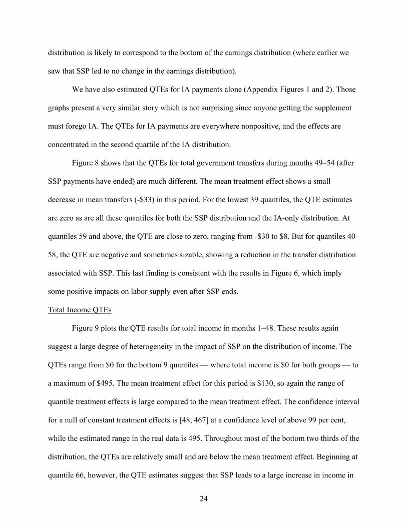
Figure 8 shows that the QTEs for total government transfers during months 49–54 (after

SSP payments have ended) are much different. The mean treatment effect shows a small

decrease in mean transfers (-$33) in this period. For the lowest 39 quantiles, the QTE estimates

are zero as are all these quantiles for both the SSP distribution and the IA-only distribution. At

quantiles 59 and above, the QTE are close to zero, ranging from -$30 to $8. But for quantiles 40–

58, the QTE are negative and sometimes sizable, showing a reduction in the transfer distribution

associated with SSP. This last finding is consistent with the results in Figure 6, which imply

some positive impacts on labor supply even after SSP ends.

Total Income QTEs

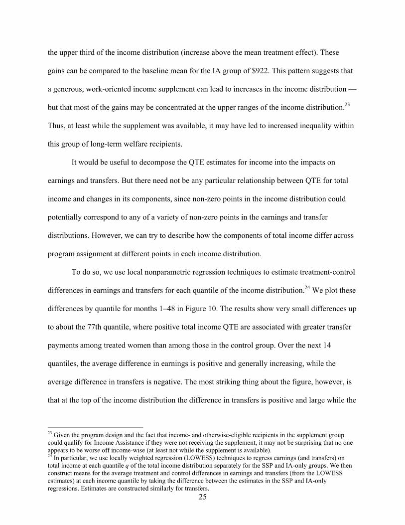
Figure 9 plots the QTE results for total income in months 1–48. These results again

suggest a large degree of heterogeneity in the impact of SSP on the distribution of income. The

QTEs range from $0 for the bottom 9 quantiles — where total income is $0 for both groups — to

a maximum of $495. The mean treatment effect for this period is $130, so again the range of

quantile treatment effects is large compared to the mean treatment effect. The confidence interval

for a null of constant treatment effects is [48, 467] at a confidence level of above 99 per cent,

while the estimated range in the real data is 495. Throughout most of the bottom two thirds of the

distribution, the QTEs are relatively small and are below the mean treatment effect. Beginning at

quantile 66, however, the QTE estimates suggest that SSP leads to a large increase in income in

25

the upper third of the income distribution (increase above the mean treatment effect). These

gains can be compared to the baseline mean for the IA group of $922. This pattern suggests that

a generous, work-oriented income supplement can lead to increases in the income distribution —

but that most of the gains may be concentrated at the upper ranges of the income distribution.23

Thus, at least while the supplement was available, it may have led to increased inequality within

this group of long-term welfare recipients.

It would be useful to decompose the QTE estimates for income into the impacts on

earnings and transfers. But there need not be any particular relationship between QTE for total

income and changes in its components, since non-zero points in the income distribution could

potentially correspond to any of a variety of non-zero points in the earnings and transfer

distributions. However, we can try to describe how the components of total income differ across

program assignment at different points in each income distribution.

To do so, we use local nonparametric regression techniques to estimate treatment-control

differences in earnings and transfers for each quantile of the income distribution.24 We plot these

differences by quantile for months 1–48 in Figure 10. The results show very small differences up

to about the 77th quantile, where positive total income QTE are associated with greater transfer

payments among treated women than among those in the control group. Over the next 14

quantiles, the average difference in earnings is positive and generally increasing, while the

average difference in transfers is negative. The most striking thing about the figure, however, is

that at the top of the income distribution the difference in transfers is positive and large while the

23 Given the program design and the fact that income- and otherwise-eligible recipients in the supplement group could qualify for Income Assistance if they were not receiving the supplement, it may not be surprising that no one appears to be worse off income-wise (at least not while the supplement is available). 24 In particular, we use locally weighted regression (LOWESS) techniques to regress earnings (and transfers) on total income at each quantile q of the total income distribution separately for the SSP and IA-only groups. We then construct means for the average treatment and control differences in earnings and transfers (from the LOWESS estimates) at each income quantile by taking the difference between the estimates in the SSP and IA-only regressions. Estimates are constructed similarly for transfers.

26

difference in earnings is negative and large. These effects are consistent with the interpretation

that the positive QTE estimates at the top of the income distribution are associated with a

combination of greater transfers and lesser earnings. We emphasize that these differences cannot

generally be interpreted as causal, since the total income quantile is not assigned experimentally.

In addition, an important drawback to this procedure is that computing average earnings at a

given total income quantile implicitly requires varying transfer payments negatively (since

transfers plus earnings are held locally fixed in such a regression).

Figure 11 plots the QTE results for the post-SSP time period, months 49–54. Here, the

impacts across the distribution are quite homogeneous, showing no change or very small changes

in the income distribution after SSP payments cease. Here the mean treatment effect of -$1

provides a fairly complete picture of the impacts during months 49–54 over almost the entire

range (with the very top of the distribution being the only real exception).

QTEs by Province

Our results in Table 2 (above) show that the mean impacts are larger and longer lasting in

New Brunswick compared to British Columbia. Here we extend that finding by comparing QTE

for the NB and BC samples. Figure 12 presents the QTE for earnings in months 1–48. To

facilitate ready comparison, we plot both the QTE for the NB sample (solid line, peaks to the

left) and the BC sample (dashed line, peaks to the right) on the same figure. For readability, we

omit the mean impacts from the figure. Figure 13 plots the difference in the QTE between the

two provinces, along with the 90 per cent confidence interval for this estimate.

These figures show that the overall pattern of the impact of SSP on the distribution of

earnings in months 1–48 is very similar — the QTEs are zero at the bottom of the distribution,

positive in the upper part of the distribution with negative or zero QTEs at the very highest

quantiles of the earnings distribution. There are qualitative differences, however. The NB sample

27

has positive QTEs in a larger range of the sample and the largest QTEs are somewhat larger in

the BC sample. Figure 13 shows that few of the pairwise differences are statistically significantly

different, however.

These differences may reflect differences in the incentives in the two provinces. The

guarantee in the IA program is much higher in BC compared to NB. The SSP benchmark,

however, was also a more generous $37,000 in BC relative to $30,000 in NB. Further, the

minimum wage was $5.50 at the beginning of the experiment in British Columbia but $5.00 in

New Brunswick. In addition, the demographic composition of the welfare population differs in

the two provinces. Sample members from British Columbia were more likely to have been born

abroad and to have completed some post-secondary education. Women selected in New

Brunswick were likely to have had longer welfare spells. One would expect earnings QTEs to be

positive first for New Brunswick simply because the minimum wage there is lower, so the lowest

earnings level at which one could obtain the supplement is lower.

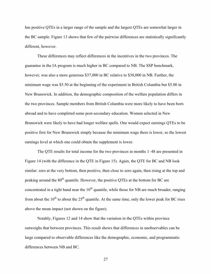
The QTE results for total income for the two provinces in months 1–48 are presented in

Figure 14 (with the difference in the QTE in Figure 15). Again, the QTE for BC and NB look

similar: zero at the very bottom, then positive, then close to zero again, then rising at the top and

peaking around the 80th quantile. However, the positive QTEs at the bottom for BC are

concentrated in a tight band near the 10th quantile, while those for NB are much broader, ranging

from about the 10th to about the 25th quantile. At the same time, only the lower peak for BC rises

above the mean impact (not shown on the figure).

Notably, Figures 12 and 14 show that the variation in the QTEs within province

outweighs that between provinces. This result shows that differences in unobservables can be

large compared to observable differences like the demographic, economic, and programmatic

differences between NB and BC.

28

The mean impacts for earnings in post-SSP period (reported in Table 2 and documented

more completely in Michalopoulos et al., 2002) suggest that earnings impacts were longer-

lasting in NB. However, earnings QTE for months 49–54 (not shown here) show a more nuanced

story: while BC does exhibit a larger range of zero QTEs compared to NB, we find that both

provinces show positive earnings impacts for a substantial portion of the distribution. The total

income QTEs in the post-SSP period (not shown here) are qualitatively similar for the two

provinces.

VII. Evidence on Rank Preservation and Rank Reversal

The QTE results provide important evidence that the impact of SSP varied across the

distribution of earnings, transfers, and income. As discussed above, the impact of the treatment

on the distribution is distinct from and generally not equal to the distribution of treatment effects.

If a person’s rank in the distribution does not change with the treatment (known as rank

preservation), however, then the impact of the treatment on the distribution would be equivalent

to the distribution of treatment effects. While we cannot test for rank preservation, we can use

the treatment and control distributions of demographic characteristics to see if there is indeed

evidence of rank reversal. For example, if the distribution of observable characteristics in some

range of the earnings distribution varies significantly between the treatment and control group,

this would be evidence against rank preservation. Unfortunately, this sort of test can provide only

negative evidence: finding no significant differences in demographics does not imply rank

preservation. To the best of our knowledge, we are the first to test for evidence of rank reversal

in this fashion.

In particular, we estimate QTEs for person averages of earnings, transfers, and income

for months 1–48. These are presented in Appendix Figures 3, 4, and 5, respectively. Note first

29

that the QTEs for the averages are more spread out than the QTEs for the person-months, as one

would expect. Also notice that the patterns are qualitatively quite similar to the person-month

estimates. We take the 25th, 50th, and 75th cutoffs for the distributions of earnings, transfers and

incomes for the treatment and control groups, and calculate mean treatment and control group

values for the various demographics within the following ranges: less than or equal to the 25th

percentile, greater than the 25th percentile but less than or equal to the 50th percentile, greater

than the 50th percentile but less than or equal to the 75th percentile, and greater than the 75th

percentile. Since the distributions of average earnings are only positive slightly below the 50th

percentile, we only calculate the tests for the 0–50th, 50th–75th, and above the 75th percentiles for

earnings. Note that we could calculate similar statistics for the person-month estimates, but find

it more transparent to use average QTEs for this purpose, because then each person only falls

within a single range. For example, one estimate of the differences is the fraction white among

treatment group members in the 25th–50th percentiles of the SSP group’s income distribution,

minus the fraction white among control group members within the analogous range.

We follow Abadie (2002) in using the bootstrap to estimate the null distribution for these

differences; our full bootstrap procedure is as follows:

1. Sampling with replacement from the actual data, draw 500 bootstrap samples,

each having the same number of observations as the real data. Index these

samples with b ∈ {1,2,…,500}.

2. For the bth replication sample, do the following:

a. Randomly order the observations in the bootstrap sample.

b. Assign the first 1,991 to a synthetic “treatment” group, and assign the rest

to a synthetic “control” group (there are 1,991 treated observations in the

actual data).

30

c. For each mean in which we are interested (for example, the fraction white

in the first 25 quantiles of the transfer distribution), calculate its value in

the synthetic program groups, and then take the difference of these sample

means. Call this difference db.

3. Sort all elements of the set {db}, b={1,2,…,500} from lowest to highest.

4. Use d25 and d475, respectively, as estimates of the 5th and 95th percentiles of the

null sampling distribution of our statistic d; a 90 per cent confidence interval is

then constructed as C=[d25, d475].

A real-data estimated difference is significantly different from zero if it falls outside the

interval C just defined. More generally, following Cameron & Trivedi (2005) we can calculate

the p-value for any statistic as follows. Create a vector of values for the statistic, including the

real data realization, with the other 500 values being the realizations of the statistic from the 500

bootstrap draws that impose the null. Take the absolute value of the statistic, and sort these

values. Let k be the index of the real data observation in the sorted data. (For example, if the real

data estimate in the sorted data lies between the 431st and 432nd bootstrap realization, then k =

432.) Then, our p-value is p = 1- (k-1)/501.

In Table 3, we present the results for 12 demographic variables for gender, race, ancestry,

language, and education. There are three panels in the table; each classifies people by their

position (quantile) in the distribution. The top panel uses the earnings distribution, the middle

panel uses the transfer distribution, and the bottom panel uses the total income distribution.25

Each column presents the difference in the demographic variable between the two samples

within a given quartile along with their p-value for statistical significance. Of the 132 differences

here, 26 are statistically significant at the 10 per cent level or below and 16 are significant at the 25 There are three columns in the top panel and four columns in the middle and bottom panels. This reflects the fact (noted above) that a larger fraction of each average earnings distribution is 0, requiring us to collapse the first and second quartiles into one group in that case.

31

5 per cent level or below. This certainly suggests some evidence of rank reversal based on these

demographic characteristics. Because we are considering multiple differences in means, simply

counting the number of rejections in these individual tests is an inadequate test: each test could

have relatively low power, a problem that can be solved with a joint test for the significance of

the twelve demographic variables in each quantile range.26

When we do joint tests for earnings, transfers, and total income over the entire period, we

find that we reject the joint test for earnings in the range 7550 ≤< q (p-value of 0.005), for

transfers in the range 250 ≤< q (p-value of 0.009), and for total income in the ranges

250 ≤< q (p-value of 0.028) and 75>q (p-value of 0.004). We fail to reject for the other 7

ranges for earnings, transfers, and total income. We also fail to reject in any ranges for IA

payments, highest monthly wage, average monthly wage, usual weekly hours, and total monthly

hours (not shown in table). While the individual tests suggest some rank reversal may be present,

the joint test results convincingly demonstrate that even at the very coarse level on which our

demographics test operates, strict rank preservation is rejected. More work — both theoretical

and empirical — would be needed to go further in discussing the degree of rank reversal, and this

issue is beyond the scope of this paper. Nonetheless, for reasons already discussed, we firmly

believe that QTE methodology is informative for evaluating programs like SSP.

26 To test for the joint significance of these differences within a given quantile range, we will use a simple chi-square test. Let the column vector of sample differences in means for the demographic characteristics be d . Each difference of means is asymptotically normal. Thus, )( ddn − is distributed N(0,V), where V is the covariance matrix for the

random variable d . Under the null hypothesis that the true vector of differences d equals zero, the statistic dVd 1−′ will have a chi-square distribution with degrees of freedom equal to the dimension of d , the vector of differences. The practical challenge is to estimate the covariance matrix; we use our realized bootstrap distribution to do so. Letting db be the realization of our vector of differences for the bth bootstrap sample, we estimate this matrix with

the estimator '*500

1

** )(*)(5001 ddddV b

bb −−= ∑

=, where ∑=

500

1

*500

1 bdd is the bootstrap-sample average of

realized differences in means. We then refer our chi-square statistics dVd 1−′ to a table of Chi-square critical values.

32

It is important to note, however, that this test is rather weak in two respects. First, for

computational ease, we have grouped many quantiles together, and we may have missed

differences in demographics within our groupings. Second, even if demographics do not change,

rank reversals may have occurred among unobservables, such as preferences for work and fixed

costs of work, for example, that are not fully reflected in observables.

Since we have found evidence of rank reversal, it suggests that our QTE estimates are

informative about the overall impacts of the program but cannot be used to determine impacts for

individuals at specific points in the distribution. Social welfare analysis, of course, makes use of

the marginal distributions shown in our QTE. Furthermore, our previous results clearly suggest

heterogeneity in the impacts of SSP even if we cannot determine exactly who is impacted by it.

VIII. Conclusions

During the 1990s, a number of governments experimented with changes to their means-

tested cash assistance programs to encourage work among low-income women. In this paper, we

investigate the impact of a unique experiment—the Canadian Self-Sufficiency Project (SSP).

SSP coupled a strict work requirement (full-time work at the minimum wage) with a generous

earnings subsidy for a period of up to 3 years for long-term Income Assistance (IA) recipients as

an alternative to simply receiving Income Assistance (IA).

Adding to the substantial literature on SSP, we examine the impacts of SSP on the

distribution of earnings, transfers (IA plus the SSP supplement), and income for long term IA

recipients using quantile treatment effects (QTEs). While mean impact analysis allows one to

calculate costs and benefits of new policies, examining impacts on the entire distribution has the

potential to uncover effects that may vary systematically across the distribution. For example,

we examine whether the benefits of SSP are spread across the distribution or concentrated in

33

particular parts of the distribution. Knowledge of such heterogeneity may be important to

policymakers, particularly in the context of programs aimed at poverty alleviation.

Our findings lead to several conclusions. First, we find quite heterogeneous impacts

across the various distributions — QTEs for earnings, transfers, and income all show

considerable variability that would be missed if we focused on simple mean treatment effects.

Moreover, these varied impacts are consistent with predictions of labor supply theory. For

example, during the period when the subsidy is available, the impact of SSP on the earnings

distribution is zero for the bottom half of the distribution. The SSP earnings distribution is higher

than the control group for much of the upper third of the distribution except at the very top,

where the earnings distribution is the same under either program or possibly lower under SSP.

Further, during the SSP receipt period, positive impacts on the transfer distribution are

concentrated at the lower end of the transfer distribution while positive impacts on the income

distribution are concentrated in the upper end of the income distribution. Impacts of SSP on these

distributions were essentially zero after the subsidy was no longer available. Variation in impacts

within province is much larger than variation between provinces.

34

References Abadie, A. (2002). Bootstrap tests for distributional treatment effects in instrumental variables models. Journal of the American Statistical Association, 97, 284–292. Ashenfelter, O. (1983). Determining participation in income-tested social programs. Journal of the American Statistical Association, 78(383), 517–525. Bargain, O., & Orsini, K. (2004). In-work policies in Europe: Killing two birds with one stone? (Discussion Paper 1445). Bonn, Germany: IZA. Barrett, G. F., Doiron, D. J., Green, D. A., & Riddell, W. C. (1996). The interaction of Unemployment Insurance and Social Assistance. (IN-AH-218E-02-96). Ottawa: Human Resources Development Canada. Bitler, M. P., Gelbach, J. B., & Hoynes, H. W. (Forthcoming). What mean impacts miss: Distributional effects of welfare reform experiments. Forthcoming, American Economic Review. Blank, R. M., Card, D., & Robins, P. K. (2000). Financial incentives for increasing work and income among low-income families. In, R. Blank & D. Card (Eds.), Finding Jobs: Work and Welfare Reform (pp. 373–419). New York, NY: Russell Sage. Blundell, R., Duncan, A., McCrae, J., & Meghir, C. (2005). Evaluating the labour market impact of Working Families’ Tax Credit using difference-in-differences. (Working Paper 4). London, United Kingdom: Analysis, HM Revenue & Customs. Blundell, R., & Hoynes, H. (2004). Has “in-work” benefit reform helped the labour market? In, D. Card, R. Blundell, & R. Freeman (Eds.), Seeking a Premier Economy: The Economic Effects of British Economic Reforms, 1980-2000 (pp. 411-459). Chicago, IL: University of Chicago Press. Brewer, M., Duncan, A., Shephard, A., & Suarez, M. (2005). Did Working Families’ Tax Credit work? The final evaluation of the impact of in-work support on parents’ labour supply and take-up behaviour in the UK. (Working Paper 2). London, United Kingdom: Analysis, HM Revenue & Customs. Cameron, A. C., & Trivedi, P. K. (2005). Microeconometrics: Methods and applications, Cambridge University Press, New York. Card, D., & Hyslop, D. (2004). Estimating the effects of a time-limited earnings subsidy for welfare-leavers. (Working Paper 10647). Cambridge, MA: NBER. Card, D., Michalopoulos, C., & Robins, P. K. (2001). The limits to wage growth: Measuring the growth rate of wages for recent welfare leavers. (Working Paper 8444). Cambridge, MA: NBER.

35

Connolly, H., & Gottschalk, P. (2003). Do earnings subsidies affect job choice? The impact of SSP supplement payments on wage growth. (SRDC Working Paper 03-02). Ottawa: Social Research and Demonstration Corporation. Eissa, N., & Hoynes, H. (Forthcoming). Behavioral responses to taxes: Lessons from the evaluation of the EITC and labor supply. Tax Policy and the Economy. Firpo, S. (2004). Efficient semiparametric estimation of quantile treatment effects. Mimeograph. Vancouver, Canada: UBC Department of Economics. Foley, K. (2004). New evidence from the Self-Sufficiency Project on the potential of earnings subsidies to increase labour force attachment among welfare recipients. (SRDC Working Paper 04-02). Ottawa: Social Research and Demonstration Corporation. Foley, K., & Schwartz, S. (2002). Leaving welfare for a job: How did SSP affect the kinds of jobs welfare recipients were willing to take? (SRDC Working Paper 02-03). Ottawa: Social Research and Demonstration Corporation. Ford, R., Gyarmati, D., Foley, K., Tattrie, D., & Jimenez, L. (2003). Can work incentives pay for themselves? Final report on the Self-Sufficiency Project for welfare applicants. Ottawa: Social Research Demonstration Corporation. Francesconi, M., & van der Klauw, W. (2004). The socioeconomic consequences of “in-work” benefit reform for British lone mothers. Mimeograph. Chapel Hill, NC: University of North Carolina at Chapel Hill. Friedlander, D., & Robins, P. K. (1997). The distributional impacts of social programs. Evaluation Review, 21(5), 531–553. Gregg, P., & Harkness, S. (2003). Welfare reform and lone parents’ employment in the UK. (Working Paper Series Number 03/072). Bristol, United Kingdom: Centre for Market and Public Organisation. Grogger, J., & Karoly, L. (2005). Welfare reform: Effects of a decade of change. Cambridge, MA: Harvard University Press. Harknett, K., & Gennetian, L. A. (2003). How an earnings supplement can affect union formation among low-income single mothers. Demography, 40(3), 458–78. Heckman, J. J., Smith, J., & Clements, N. (1997). Making the most out of programme evaluations and social experiments: Accounting for heterogeneity in programme impacts. Review of Economic Studies, 64, 487–535. Hotz, V. J., & Scholz, J. K. (2003). The Earned Income Tax Credit. In, R. Moffitt, (Ed.), Means tested transfer programs in the United States (pp. 141–197). Chicago, IL: The University of Chicago Press.

36

Imbens, G. W., & Angrist, J. D. (1994). Identification and estimation of local average treatment effects. Econometrica, 62(2), 467–75. Kamionka, T., & Lacroix, G. (2003). Assessing the impact of non-response on the treatment effect in the Canadian Self-Sufficiency Project. (SRDC Working Paper Number 03-05). Ottawa: Social Research and Demonstration Corporation. Leigh, A. (2004). Optimal design of Earned Income Tax Credits: Evidence from a British natural experiment. Mimeograph. Canberra, Australia: Australian National University. Lise, J., Seitz, S., & Smith, J. (2005). Equilibrium policy experiments and the evaluation of social programs. Mimeograph. Kingston, Ontario: Queen’s University. Michalopoulos, C., Tattrie, D., Miller, C., Robins, P. K., Morris, P., Gyarmati, D., Redcross, C., Foley, K., & Ford, D. (2002). Making work pay: Final report on the Self-Sufficiency Project for long-term welfare recipients. Social Research and Demonstration Corporation. Michalopoulos, C., Card, D., Gennetian, L., Harknett, K., and Robins, P. (2000). The Self Sufficiency Project at 36 Months: Effects of a Financial Work Incentive on Employment and Income. Social Research and Demonstration Corporation. Michalopoulos, C., Robins, P., & Card, D. (2005). "When financial work incentives pay for themselves: evidence from a randomized social experiment for welfare recipients," Journal of Public Economics, 89(1), 5–29. Owens, J. (2005). Fundamental Tax Reform: The Experience of OECD Countries. (Background Paper Number 47). Washington, DC: Tax Foundation. Smith, N., Dex, S., Vlasblom, J., & Callan, T. (2003). The effects of taxation on married women’s labour supply across four countries. Oxford Economic Papers, 55(3), 417–439. Wooldridge, J. M. (2003). Inverse Probability Weighted Estimation for General Missing Data Problems. Mimeograph. East Lansing, MI: Michigan State University. Zabel, J., Schwartz, S., & Donald, S. (2004). An econometric analysis of the impact of the Self-Sufficiency Project on unemployment and employment durations. (SRDC Working Paper 04-05). Ottawa: Social Research and Demonstration Corporation.

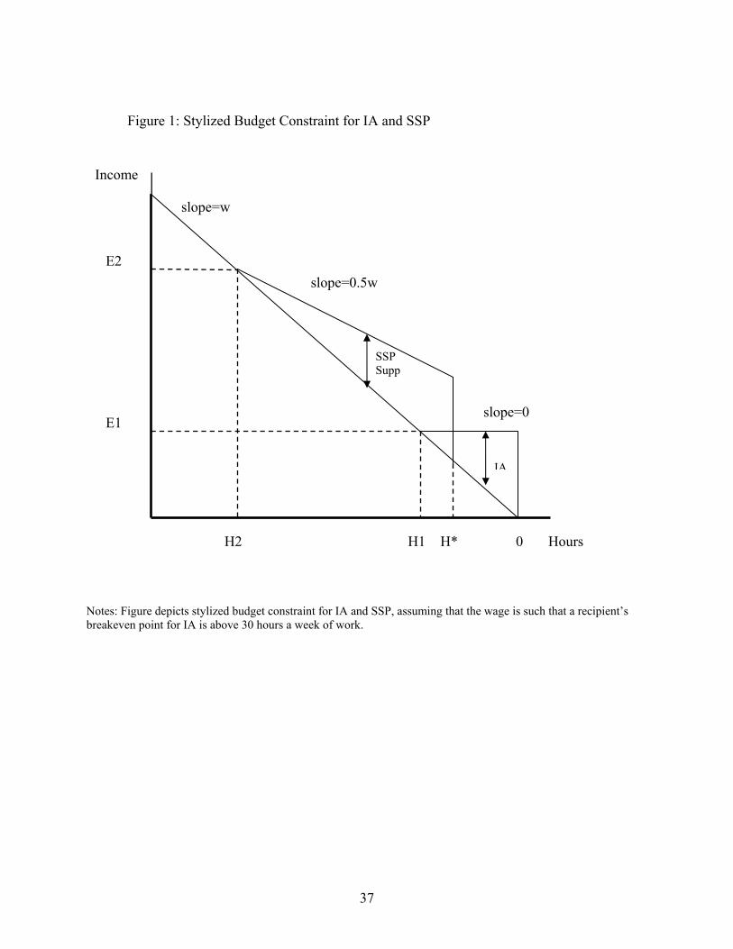
37

Notes: Figure depicts stylized budget constraint for IA and SSP, assuming that the wage is such that a recipient’s breakeven point for IA is above 30 hours a week of work.

slope=w

SSP Supp

IA

slope=0

slope=0.5w

Hours H1

E2

H* H2

Figure 1: Stylized Budget Constraint for IA and SSP

0

Income

E1

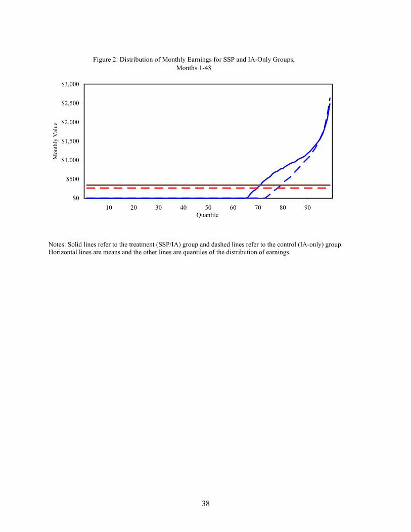
38

Notes: Solid lines refer to the treatment (SSP/IA) group and dashed lines refer to the control (IA-only) group. Horizontal lines are means and the other lines are quantiles of the distribution of earnings.

Figure 2: Distribution of Monthly Earnings for SSP and IA-Only Groups, Months 1-48

$0

$500

$1,000

$1,500

$2,000

$2,500

$3,000

10 20 30 40 50 60 70 80 90Quantile

Mon

thly

Val

ue

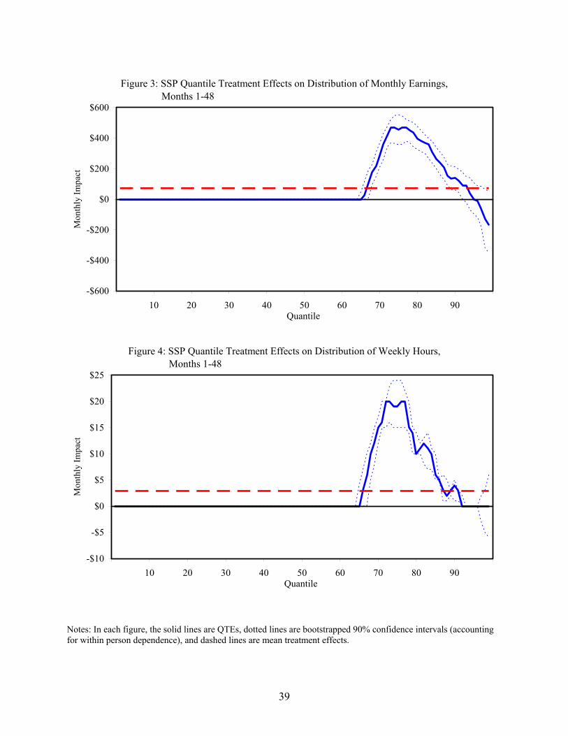
39

Notes: In each figure, the solid lines are QTEs, dotted lines are bootstrapped 90% confidence intervals (accounting for within person dependence), and dashed lines are mean treatment effects.

Figure 3: SSP Quantile Treatment Effects on Distribution of Monthly Earnings, Months 1-48

-$600

-$400

-$200

$0

$200

$400

$600

10 20 30 40 50 60 70 80 90Quantile

Mon

thly

Impa

ct

Figure 4: SSP Quantile Treatment Effects on Distribution of Weekly Hours, Months 1-48

-$10

-$5

$0

$5

$10

$15

$20

$25

10 20 30 40 50 60 70 80 90Quantile

Mon

thly

Impa

ct

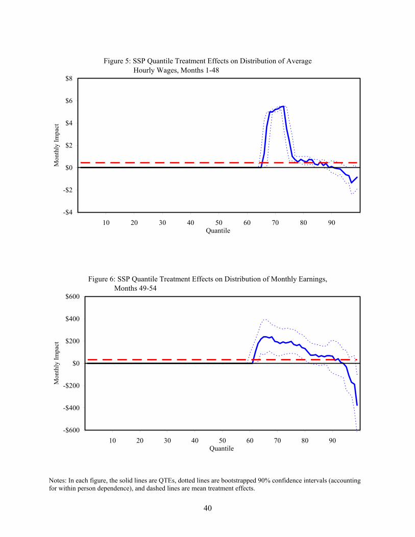
40

Notes: In each figure, the solid lines are QTEs, dotted lines are bootstrapped 90% confidence intervals (accounting for within person dependence), and dashed lines are mean treatment effects.

Figure 6: SSP Quantile Treatment Effects on Distribution of Monthly Earnings, Months 49-54

-$600

-$400

-$200

$0

$200

$400

$600

10 20 30 40 50 60 70 80 90Quantile

Mon

thly

Impa

ctFigure 5: SSP Quantile Treatment Effects on Distribution of Average Hourly Wages, Months 1-48

-$4

-$2

$0

$2

$4

$6

$8

10 20 30 40 50 60 70 80 90Quantile

Mon

thly

Impa

ct

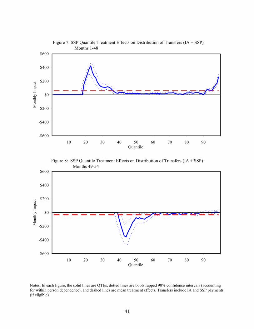
41

Notes: In each figure, the solid lines are QTEs, dotted lines are bootstrapped 90% confidence intervals (accounting for within person dependence), and dashed lines are mean treatment effects. Transfers include IA and SSP payments (if eligible).

Figure 7: SSP Quantile Treatment Effects on Distribution of Transfers (IA + SSP) Months 1-48

-$600

-$400

-$200

$0

$200

$400

$600

10 20 30 40 50 60 70 80 90Quantile

Mon

thly

Impa

ct

Figure 8: SSP Quantile Treatment Effects on Distribution of Transfers (IA + SSP) Months 49-54

-$600

-$400

-$200

$0

$200

$400

$600

10 20 30 40 50 60 70 80 90Quantile

Mon

thly

Impa

ct

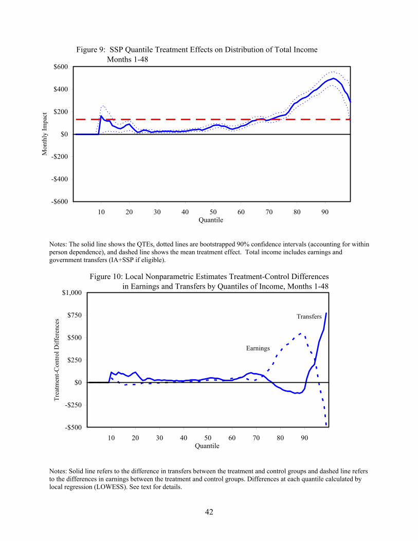
42

Notes: The solid line shows the QTEs, dotted lines are bootstrapped 90% confidence intervals (accounting for within person dependence), and dashed line shows the mean treatment effect. Total income includes earnings and government transfers (IA+SSP if eligible).

Notes: Solid line refers to the difference in transfers between the treatment and control groups and dashed line refers to the differences in earnings between the treatment and control groups. Differences at each quantile calculated by local regression (LOWESS). See text for details.

Figure 9: SSP Quantile Treatment Effects on Distribution of Total Income Months 1-48

-$600

-$400

-$200

$0

$200

$400

$600

10 20 30 40 50 60 70 80 90Quantile

Mon

thly

Impa

ct

Figure 10: Local Nonparametric Estimates Treatment-Control Differences in Earnings and Transfers by Quantiles of Income, Months 1-48

-$500

-$250

$0

$250

$500

$750

$1,000

10 20 30 40 50 60 70 80 90Quantile

Trea

tmen

t-Con

trol D

iffer

ence

s

Earnings

Transfers

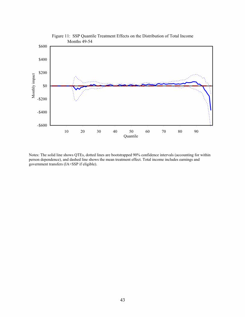
43

Notes: The solid line shows QTEs, dotted lines are bootstrapped 90% confidence intervals (accounting for within person dependence), and dashed line shows the mean treatment effect. Total income includes earnings and government transfers (IA+SSP if eligible).

Figure 11: SSP Quantile Treatment Effects on the Distribution of Total Income Months 49-54

-$600

-$400

-$200

$0

$200

$400

$600

10 20 30 40 50 60 70 80 90Quantile

Mon

thly

impa

ct

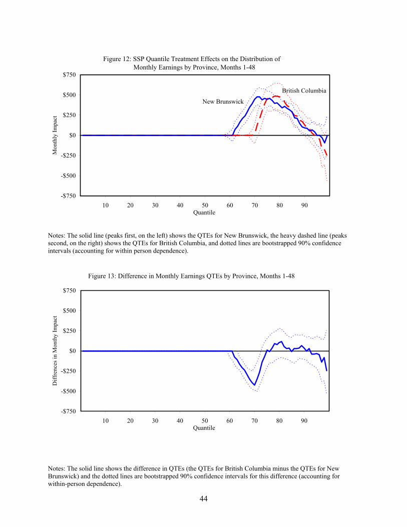
44

Notes: The solid line (peaks first, on the left) shows the QTEs for New Brunswick, the heavy dashed line (peaks second, on the right) shows the QTEs for British Columbia, and dotted lines are bootstrapped 90% confidence intervals (accounting for within person dependence).

Notes: The solid line shows the difference in QTEs (the QTEs for British Columbia minus the QTEs for New Brunswick) and the dotted lines are bootstrapped 90% confidence intervals for this difference (accounting for within-person dependence).

Figure 13: Difference in Monthly Earnings QTEs by Province, Months 1-48

-$750

-$500

-$250

$0

$250

$500

$750

10 20 30 40 50 60 70 80 90Quantile

Diff

renc

es in

Mon

thy

Impa

ctFigure 12: SSP Quantile Treatment Effects on the Distribution of Monthly Earnings by Province, Months 1-48

-$750

-$500

-$250

$0

$250

$500

$750

10 20 30 40 50 60 70 80 90Quantile

Mon

thly

Impa

ct

New Brunswick

British Columbia

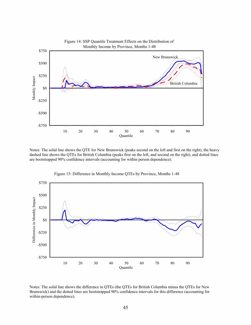
45

Notes: The solid line shows the QTE for New Brunswick (peaks second on the left and first on the right), the heavy dashed line shows the QTEs for British Columbia (peaks first on the left, and second on the right), and dotted lines are bootstrapped 90% confidence intervals (accounting for within person dependence).

Notes: The solid line shows the difference in QTEs (the QTEs for British Columbia minus the QTEs for New Brunswick) and the dotted lines are bootstrapped 90% confidence intervals for this difference (accounting for within-person dependence).

Figure 15: Difference in Monthly Income QTEs by Province, Months 1-48

-$750

-$500

-$250

$0

$250

$500

$750

10 20 30 40 50 60 70 80 90Quantile

Diff

eren

ces i

n M

onth

ly Im

pact

Figure 14: SSP Quantile Treatment Effects on the Distribution of Monthly Income by Province, Months 1-48

-$750

-$500

-$250

$0

$250

$500

$750

10 20 30 40 50 60 70 80 90Quantile

Mon

thly

Impa

ct

New Brunswick

British Columbia

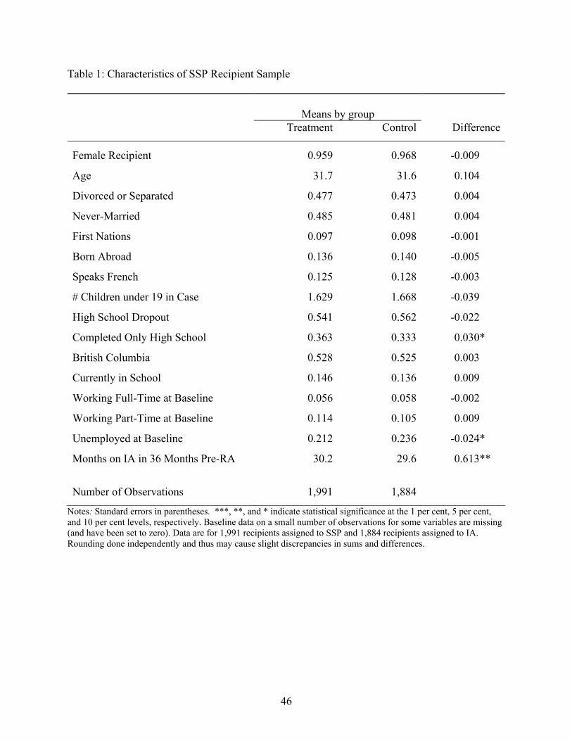
46

Table 1: Characteristics of SSP Recipient Sample

Means by group

Treatment Control Difference

Female Recipient 0.959 0.968 -0.009

Age 31.7 31.6 0.104

Divorced or Separated 0.477 0.473 0.004

Never-Married 0.485 0.481 0.004

First Nations 0.097 0.098 -0.001

Born Abroad 0.136 0.140 -0.005

Speaks French 0.125 0.128 -0.003

# Children under 19 in Case 1.629 1.668 -0.039

High School Dropout 0.541 0.562 -0.022

Completed Only High School 0.363 0.333 0.030*

British Columbia 0.528 0.525 0.003

Currently in School 0.146 0.136 0.009

Working Full-Time at Baseline 0.056 0.058 -0.002

Working Part-Time at Baseline 0.114 0.105 0.009

Unemployed at Baseline 0.212 0.236 -0.024*

Months on IA in 36 Months Pre-RA 30.2 29.6 0.613**

Number of Observations 1,991 1,884

Notes: Standard errors in parentheses. ***, **, and * indicate statistical significance at the 1 per cent, 5 per cent, and 10 per cent levels, respectively. Baseline data on a small number of observations for some variables are missing (and have been set to zero). Data are for 1,991 recipients assigned to SSP and 1,884 recipients assigned to IA. Rounding done independently and thus may cause slight discrepancies in sums and differences.

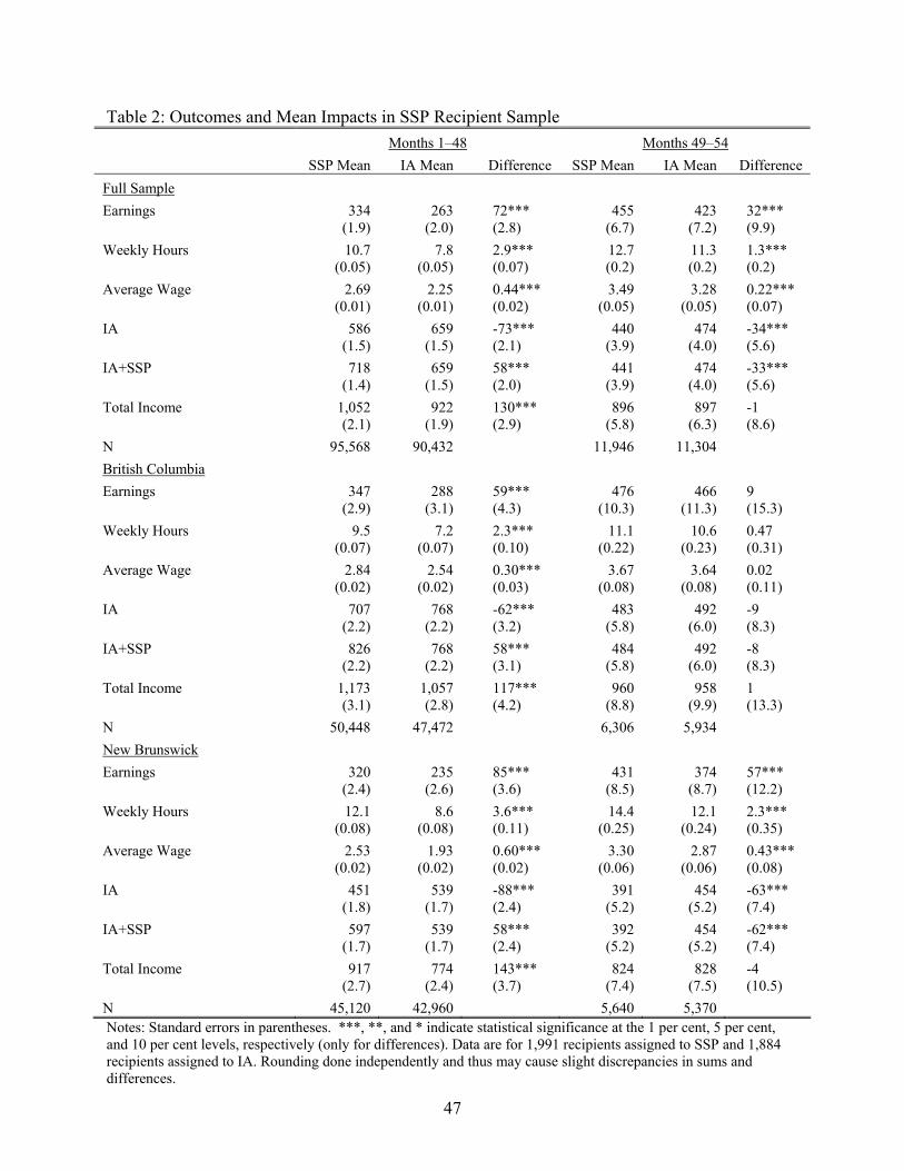
47

Table 2: Outcomes and Mean Impacts in SSP Recipient Sample Months 1–48 Months 49–54 SSP Mean IA Mean Difference SSP Mean IA Mean Difference Full Sample Earnings 334

(1.9) 263

(2.0) 72*** (2.8)

455 (6.7)

423 (7.2)

32*** (9.9)

Weekly Hours 10.7 (0.05)

7.8 (0.05)

2.9*** (0.07)

12.7 (0.2)

11.3 (0.2)

1.3*** (0.2)

Average Wage 2.69 (0.01)

2.25 (0.01)

0.44*** (0.02)

3.49 (0.05)

3.28 (0.05)

0.22*** (0.07)

IA 586 (1.5)

659 (1.5)

-73*** (2.1)

440 (3.9)

474 (4.0)

-34*** (5.6)

IA+SSP 718 (1.4)

659 (1.5)

58*** (2.0)

441 (3.9)

474 (4.0)

-33*** (5.6)

Total Income 1,052 (2.1)

922 (1.9)

130*** (2.9)

896 (5.8)

897 (6.3)

-1 (8.6)

N 95,568 90,432 11,946 11,304 British Columbia Earnings 347

(2.9) 288

(3.1) 59*** (4.3)

476 (10.3)

466 (11.3)

9 (15.3)

Weekly Hours 9.5 (0.07)

7.2 (0.07)

2.3*** (0.10)

11.1 (0.22)

10.6 (0.23)

0.47 (0.31)

Average Wage 2.84 (0.02)

2.54 (0.02)

0.30*** (0.03)

3.67 (0.08)

3.64 (0.08)

0.02 (0.11)

IA 707 (2.2)

768 (2.2)

-62*** (3.2)

483 (5.8)

492 (6.0)

-9 (8.3)

IA+SSP 826 (2.2)

768 (2.2)

58*** (3.1)

484 (5.8)

492 (6.0)

-8 (8.3)

Total Income 1,173 (3.1)

1,057 (2.8)

117*** (4.2)

960 (8.8)

958 (9.9)

1 (13.3)

N 50,448 47,472 6,306 5,934 New Brunswick Earnings 320

(2.4) 235

(2.6) 85*** (3.6)

431 (8.5)

374 (8.7)

57*** (12.2)

Weekly Hours 12.1 (0.08)

8.6 (0.08)

3.6*** (0.11)

14.4 (0.25)

12.1 (0.24)

2.3*** (0.35)

Average Wage 2.53 (0.02)

1.93 (0.02)

0.60*** (0.02)

3.30 (0.06)

2.87 (0.06)

0.43*** (0.08)

IA 451 (1.8)

539 (1.7)

-88*** (2.4)

391 (5.2)

454 (5.2)

-63*** (7.4)

IA+SSP 597 (1.7)

539 (1.7)

58*** (2.4)

392 (5.2)

454 (5.2)

-62*** (7.4)

Total Income 917 (2.7)

774 (2.4)

143*** (3.7)

824 (7.4)

828 (7.5)

-4 (10.5)

N 45,120 42,960 5,640 5,370 Notes: Standard errors in parentheses. ***, **, and * indicate statistical significance at the 1 per cent, 5 per cent, and 10 per cent levels, respectively (only for differences). Data are for 1,991 recipients assigned to SSP and 1,884 recipients assigned to IA. Rounding done independently and thus may cause slight discrepancies in sums and differences.

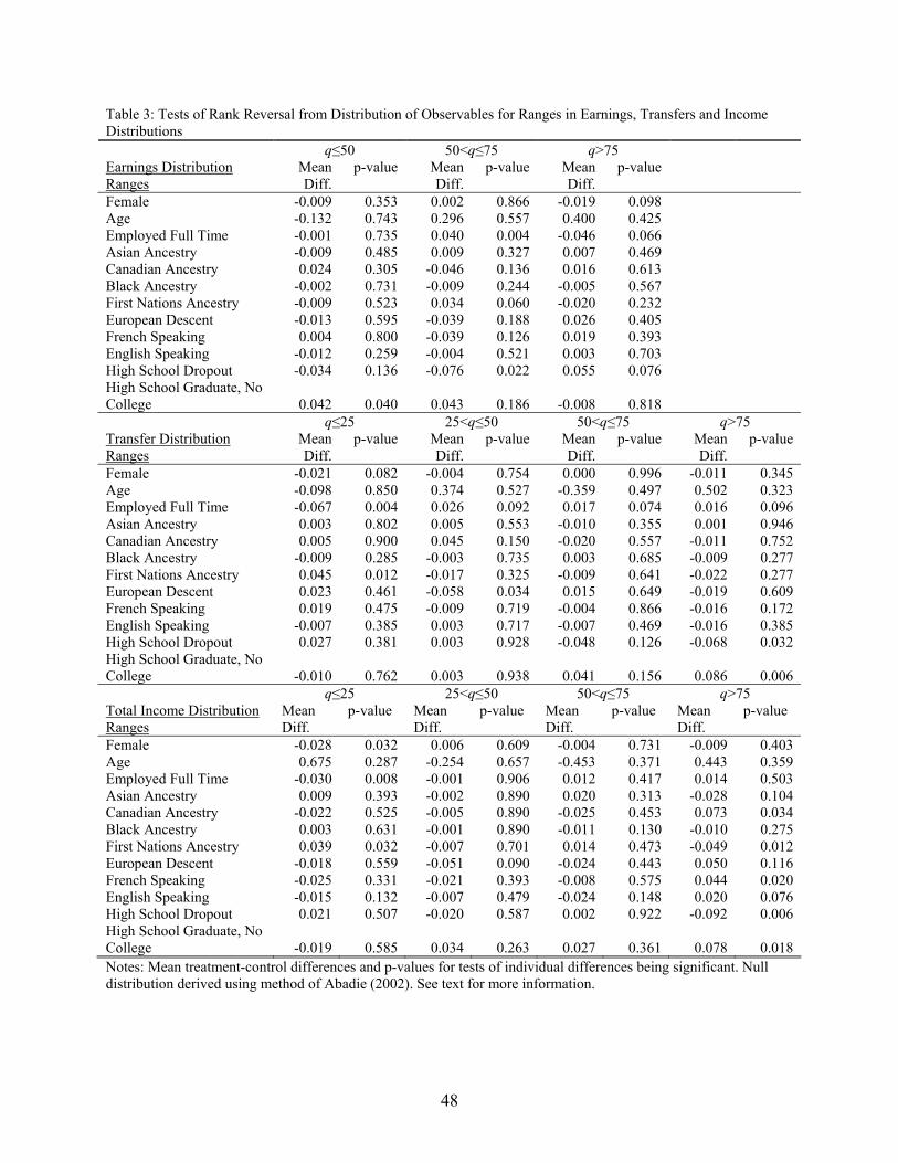
48

Table 3: Tests of Rank Reversal from Distribution of Observables for Ranges in Earnings, Transfers and Income Distributions

q≤50 50<q≤75 q>75 Earnings Distribution Ranges

Mean Diff.

p-value Mean Diff.

p-value Mean Diff.

p-value

Female -0.009 0.353 0.002 0.866 -0.019 0.098 Age -0.132 0.743 0.296 0.557 0.400 0.425 Employed Full Time -0.001 0.735 0.040 0.004 -0.046 0.066 Asian Ancestry -0.009 0.485 0.009 0.327 0.007 0.469 Canadian Ancestry 0.024 0.305 -0.046 0.136 0.016 0.613 Black Ancestry -0.002 0.731 -0.009 0.244 -0.005 0.567 First Nations Ancestry -0.009 0.523 0.034 0.060 -0.020 0.232 European Descent -0.013 0.595 -0.039 0.188 0.026 0.405 French Speaking 0.004 0.800 -0.039 0.126 0.019 0.393 English Speaking -0.012 0.259 -0.004 0.521 0.003 0.703 High School Dropout -0.034 0.136 -0.076 0.022 0.055 0.076 High School Graduate, No College 0.042 0.040 0.043 0.186 -0.008 0.818

q≤25 25<q≤50 50<q≤75 q>75 Transfer Distribution Ranges

Mean Diff.

p-value Mean Diff.

p-value Mean Diff.

p-value Mean Diff.

p-value

Female -0.021 0.082 -0.004 0.754 0.000 0.996 -0.011 0.345 Age -0.098 0.850 0.374 0.527 -0.359 0.497 0.502 0.323 Employed Full Time -0.067 0.004 0.026 0.092 0.017 0.074 0.016 0.096 Asian Ancestry 0.003 0.802 0.005 0.553 -0.010 0.355 0.001 0.946 Canadian Ancestry 0.005 0.900 0.045 0.150 -0.020 0.557 -0.011 0.752 Black Ancestry -0.009 0.285 -0.003 0.735 0.003 0.685 -0.009 0.277 First Nations Ancestry 0.045 0.012 -0.017 0.325 -0.009 0.641 -0.022 0.277 European Descent 0.023 0.461 -0.058 0.034 0.015 0.649 -0.019 0.609 French Speaking 0.019 0.475 -0.009 0.719 -0.004 0.866 -0.016 0.172 English Speaking -0.007 0.385 0.003 0.717 -0.007 0.469 -0.016 0.385 High School Dropout 0.027 0.381 0.003 0.928 -0.048 0.126 -0.068 0.032 High School Graduate, No College -0.010 0.762 0.003 0.938 0.041 0.156 0.086 0.006

q≤25 25<q≤50 50<q≤75 q>75 Total Income Distribution Ranges

Mean Diff.

p-value Mean Diff.

p-value Mean Diff.

p-value Mean Diff.

p-value

Female -0.028 0.032 0.006 0.609 -0.004 0.731 -0.009 0.403 Age 0.675 0.287 -0.254 0.657 -0.453 0.371 0.443 0.359 Employed Full Time -0.030 0.008 -0.001 0.906 0.012 0.417 0.014 0.503 Asian Ancestry 0.009 0.393 -0.002 0.890 0.020 0.313 -0.028 0.104 Canadian Ancestry -0.022 0.525 -0.005 0.890 -0.025 0.453 0.073 0.034 Black Ancestry 0.003 0.631 -0.001 0.890 -0.011 0.130 -0.010 0.275 First Nations Ancestry 0.039 0.032 -0.007 0.701 0.014 0.473 -0.049 0.012 European Descent -0.018 0.559 -0.051 0.090 -0.024 0.443 0.050 0.116 French Speaking -0.025 0.331 -0.021 0.393 -0.008 0.575 0.044 0.020 English Speaking -0.015 0.132 -0.007 0.479 -0.024 0.148 0.020 0.076 High School Dropout 0.021 0.507 -0.020 0.587 0.002 0.922 -0.092 0.006 High School Graduate, No College -0.019 0.585 0.034 0.263 0.027 0.361 0.078 0.018 Notes: Mean treatment-control differences and p-values for tests of individual differences being significant. Null distribution derived using method of Abadie (2002). See text for more information.

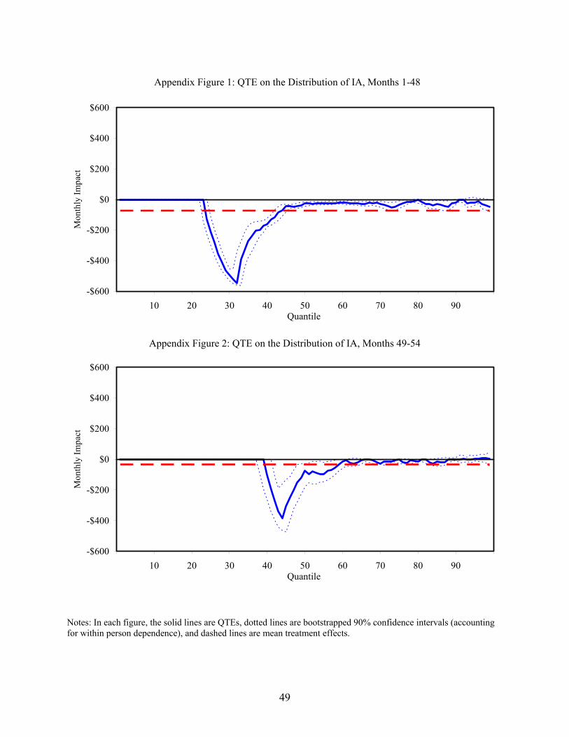
49

Notes: In each figure, the solid lines are QTEs, dotted lines are bootstrapped 90% confidence intervals (accounting for within person dependence), and dashed lines are mean treatment effects.

Appendix Figure 1: QTE on the Distribution of IA, Months 1-48

-$600

-$400

-$200

$0

$200

$400

$600

10 20 30 40 50 60 70 80 90Quantile

Mon

thly

Impa

ct

Appendix Figure 2: QTE on the Distribution of IA, Months 49-54

-$600

-$400

-$200

$0

$200

$400

$600

10 20 30 40 50 60 70 80 90Quantile

Mon

thly

Impa

ct

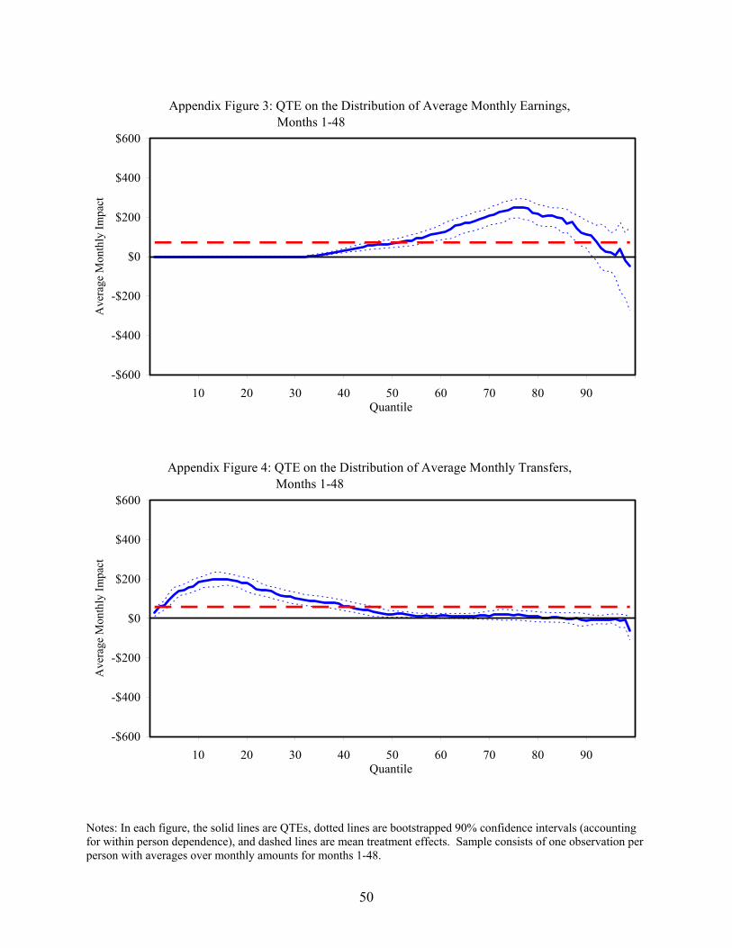
50

Notes: In each figure, the solid lines are QTEs, dotted lines are bootstrapped 90% confidence intervals (accounting for within person dependence), and dashed lines are mean treatment effects. Sample consists of one observation per person with averages over monthly amounts for months 1-48.

Appendix Figure 3: QTE on the Distribution of Average Monthly Earnings, Months 1-48

-$600

-$400

-$200

$0

$200

$400

$600

10 20 30 40 50 60 70 80 90Quantile

Ave

rage

Mon

thly

Impa

ct

Appendix Figure 4: QTE on the Distribution of Average Monthly Transfers, Months 1-48

-$600

-$400

-$200

$0

$200

$400

$600

10 20 30 40 50 60 70 80 90Quantile

Ave

rage

Mon

thly

Impa

ct

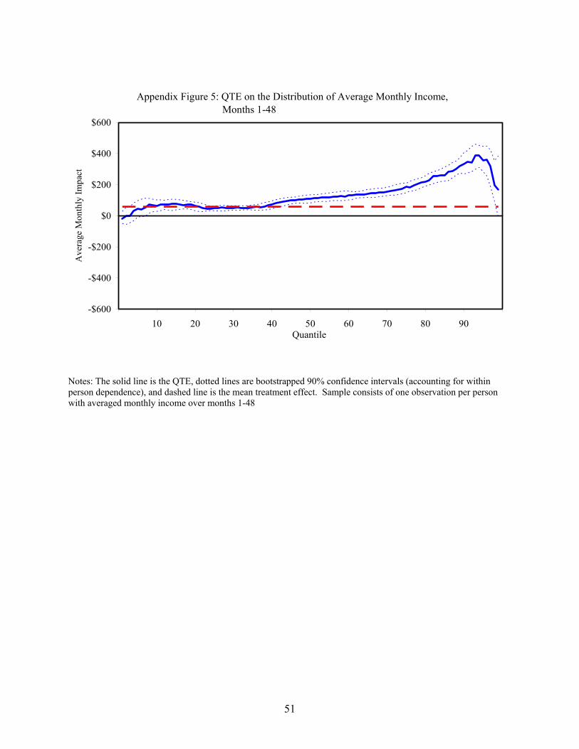
51

Notes: The solid line is the QTE, dotted lines are bootstrapped 90% confidence intervals (accounting for within person dependence), and dashed line is the mean treatment effect. Sample consists of one observation per person with averaged monthly income over months 1-48

Appendix Figure 5: QTE on the Distribution of Average Monthly Income, Months 1-48

-$600

-$400

-$200

$0

$200

$400

$600

10 20 30 40 50 60 70 80 90Quantile

Ave

rage

Mon

thly

Impa

ct