* Contact: Matthias Burgert, Swiss National Bank, matthias.burgert@snb.ch; Werner Roeger, European Commission, Directorate-General for Economic and Financial Affairs, werner.roeger@ec.europa.eu. We are grateful to Jan in'tVeld for valuable comments. This paper has been largely written while Matthias Burgert was working with the Directorate-General for Economic and Financial Affairs. The content of this paper does not reflect views of the Swiss National Bank or the European Commission.

Fiscal policy in EMU with downward nominal wage rigidity

Matthias Burgert and Werner Roeger*

15 May 2017

Abstract

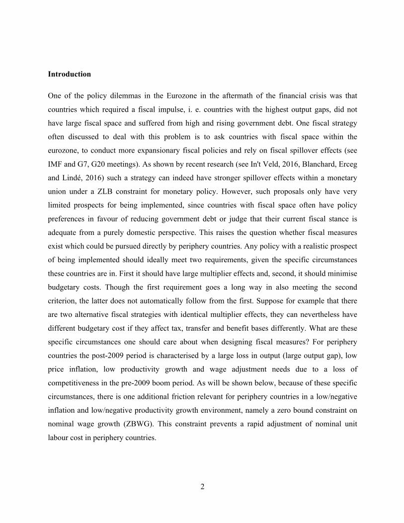
There is considerable empirical evidence for downward nominal wage rigidity in EMU countries in the recent bust episode. We use a three region (EA periphery-RoEA-RoW) DSGE model to analyse two alternative fiscal strategies for an individual country in EMU, namely an increase in government expenditure vs. a reduction in revenues, via a cut in employers’ social security contributions. Both fiscal strategies have been advocated as possible instruments in the current juncture. An expenditure increase can especially be effective under a ZLB constraint since it raises inflation. A cut in SSC is targeting the constraint on wage inflation and facilitates labour market clearing. It is shown that for an open economy in EMU the latter fiscal strategy is superior along two dimensions. First the fiscal multiplier is larger and second, the budgetary costs are smaller because the adjustment of the economy to a SSC reduction is more tax rich. These two features strongly reduce the budgetary cost and make this policy measure attractive for a number of periphery countries which suffer from very limited fiscal space.

2

Introduction

One of the policy dilemmas in the Eurozone in the aftermath of the financial crisis was that

countries which required a fiscal impulse, i. e. countries with the highest output gaps, did not

have large fiscal space and suffered from high and rising government debt. One fiscal strategy

often discussed to deal with this problem is to ask countries with fiscal space within the

eurozone, to conduct more expansionary fiscal policies and rely on fiscal spillover effects (see

IMF and G7, G20 meetings). As shown by recent research (see In't Veld, 2016, Blanchard, Erceg

and Lindé, 2016) such a strategy can indeed have stronger spillover effects within a monetary

union under a ZLB constraint for monetary policy. However, such proposals only have very

limited prospects for being implemented, since countries with fiscal space often have policy

preferences in favour of reducing government debt or judge that their current fiscal stance is

adequate from a purely domestic perspective. This raises the question whether fiscal measures

exist which could be pursued directly by periphery countries. Any policy with a realistic prospect

of being implemented should ideally meet two requirements, given the specific circumstances

these countries are in. First it should have large multiplier effects and, second, it should minimise

budgetary costs. Though the first requirement goes a long way in also meeting the second

criterion, the latter does not automatically follow from the first. Suppose for example that there

are two alternative fiscal strategies with identical multiplier effects, they can nevertheless have

different budgetary cost if they affect tax, transfer and benefit bases differently. What are these

specific circumstances one should care about when designing fiscal measures? For periphery

countries the post-2009 period is characterised by a large loss in output (large output gap), low

price inflation, low productivity growth and wage adjustment needs due to a loss of

competitiveness in the pre-2009 boom period. As will be shown below, because of these specific

circumstances, there is one additional friction relevant for periphery countries in a low/negative

inflation and low/negative productivity growth environment, namely a zero bound constraint on

nominal wage growth (ZBWG). This constraint prevents a rapid adjustment of nominal unit

labour cost in periphery countries.

3

Fiscal policy discussions at the current juncture usually focus on the ZLB constraint on the

policy rate and advocate raising government expenditure because of the higher fiscal expenditure

multiplier implied by the ZLB (see Coenen et al., 2012, Christiano et al., 2011). Coenen et al.

(2012) show that an expenditure increase yields larger multipliers compared to a revenue

reduction. However, there remains uncertainty about the inflationary impact of such measures

(see discussion of Blanchard et al. (2016) by Uhlig (2016) and Linde and Trabandt (2016)).

Second, the multiplier effect is often discussed in a closed economy context and disregards open

economy aspects such as detrimental effects of inflation on competitiveness. Because of the

latter, Farhi and Werning (2014) argue that the fiscal spending multiplier in open economies

within a monetary union is likely to be smaller than one, since the real interest rate reducing

effect of spending will be largely offset by competitiveness losses.

In this paper, we extent the discussion of fiscal policy in individual countries of EMU by also

taking into account the ZBWG constraint. In this context we take up the discussion again on the

relative effectiveness of an increase in spending vs a cut in revenues. In particular, we compare

two types of policies to each other, namely an increase in government purchases and a reduction

of employer’s social security contributions (SSC). The ZBWG constraint will likely have

ambiguous consequences for the open economy spending multiplier. On the one hand, it reduces

the inflation effect of the fiscal shock and therefore further reduces the domestic demand

stimulus via the expected real interest rate channel, on the other hand, it mitigates adverse

competitiveness effects.

Wage subsidies for firms has been proposed by Schmitt-Grohe and Uribe (2015). This policy

measure targets the wage adjustment friction in the labour market directly but does not exploit

the ZLB constraint. However, since inflation has ambiguous effects on the fiscal multiplier in

open economies, a policy which targets the ZBWG friction instead of the ZLB constraint may be

more efficient for an open economy in a monetary union.

We take up this issue and compare the effects of a temporary expenditure increase vs. a

temporary reduction of social security contributions paid by firms in the context of a fully

specified 3-region DSGE model of the eurozone periphery, the rest of the eurozone and the rest

of the world. The model features a standard wage setting rule, which exhibits nominal and real

4

wage adjustment frictions. We add to these wage frictions a downward nominal wage rigidity.

We model this friction as a partially binding constraint. In order to implement this we create a

deflationary crisis baseline with a fall in output and inflation similar to what has been

experienced in the EA periphery.

The structure of the paper is as follows. Section 1 provides some empirical evidence that wage

inflation is constrained around zero in EA periphery countries. Section 2 presents the model and

discusses the type of wage frictions we are considering. Section 3 presents a baseline scenario,

where we give positive and negative demand shocks, in order to generate a boom and a bust in

the order of magnitude as observed for EA periphery countries. Section 4 discusses fiscal policy

options for periphery countries within EMU. Essentially we compare GDP effects and budgetary

costs of a temporary increase in public consumption with a temporary reduction of employers'

social security contributions. Both measures are ex ante identical. In order to identify the impact

of the wage friction we compare both policies with and without zero bound on wages. Section 5

concludes.

1. Empirical Evidence on downward nominal wage rigidity

The presence of downward nominal wage rigidity is often discussed in the economics literature.

For example, Holden and Wulfsberg (2008) provide evidence for downward nominal wage

rigidity for OECD countries in the pre-2009 period. Given the low inflation in the aftermath of

the 2009 financial crisis this phenomenon appears more acute now. Schmitt-Grohe and Uribe

(2016) provide empirical evidence that nominal rigidity may have indeed been prevalent in the

post-2009 years. Using Data on nominal average hourly labour cost in manufacturing,

construction and services they show positive wage growth in Ireland, Italy, Spain and Portugal

over the period 2008Q1 to 2011Q2 despite strongly rising unemployment rates over the same

period. The OECD economic outlook 2014 also provides micro evidence for increased nominal

downward wage rigidity in Greece, Portugal and Spain. Using administrative data for Spain it is

shown that the incidence of wage freezes at zero increased from 3% in 2008 to 22% in 2012. A

survey conducted in 2009 by the Wage Dynamics Network (WDN) of European central banks

also comes to the conclusion that downward wage rigidity is prevalent. Only a small percentage

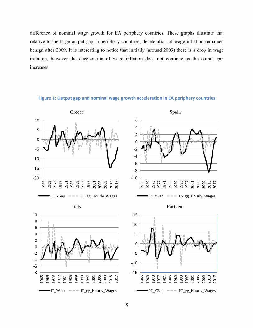
of firms reported cuts in base wages (see ECB 2012). Figure 1 shows output gaps and the first

5

difference of nominal wage growth for EA periphery countries. These graphs illustrate that

relative to the large output gap in periphery countries, deceleration of wage inflation remained

benign after 2009. It is interesting to notice that initially (around 2009) there is a drop in wage

inflation, however the deceleration of wage inflation does not continue as the output gap

increases.

Figure1:OutputgapandnominalwagegrowthaccelerationinEAperipherycountries

Greece Spain

Italy Portugal

-20

-15

-10

-5

0

5

10

1965

1969

1973

1977

1981

1985

1989

1993

1997

2001

2005

2009

2013

2017

EL_YGap EL_gg_Hourly_Wages

-10 -8 -6 -4 -2 0

2

4

6

1965

1969

1973

1977

1981

1985

1989

1993

1997

2001

2005

2009

2013

2017

ES_YGap ES_gg_Hourly_Wages

-8 -6 -4 -2 02468

10

1965

1969

1973

1977

1981

1985

1989

1993

1997

2001

2005

2009

2013

2017

IT_YGap IT_gg_Hourly_Wages

-15

-10

-5

0

5

10

15

1965

1969

1973

1977

1981

1985

1989

1993

1997

2001

2005

2009

2013

2017

PT_YGap PT_gg_Hourly_Wages

6

Source: AMECO, European Commission

Taking Italy as an example, compared to previous recessions around 1982 and 1993, which were

associated with a deceleration of nominal wage growth, such a deceleration did not occur after

2008, despite the large and long output gap Italy experienced.

2. Model and Wage rule

For our analysis we use a three region DSGE model and we distinguish between a representative

EA periphery country, the rest of the Euro area and the rest of the world. A detailed model

description and calibration is contained in the appendix of this paper. In this section we

concentrate on the description of the wage Phillips curve and the non-linearity imposed by the

ZBWG.

We assume that trade union set wages according to the standard Phillips curve mechanism. They

target real consumption wages (𝑊"/𝑃"%) in the medium term to be consistent with the marginal

rate of substitution between leisure and consumption of a weighted average of constrained and

unconstrained households. There are two types of adjustment frictions which prevent a rapid

adjustment of real wages. First, because of wage contracts with duration of more than one

quarter there is a nominal wage friction. In addition, there is often habit persistence in wage

setting which restricts fluctuations of real wage growth (adjusted for trend productivity growth)

(see Blanchard et al., 2015). Both constraints are operative in the standard model. In this paper

we consider an additional constraint on nominal wage adjustment, namely a floor on nominal

wage growth at zero, which is likely to be relevant for a number of periphery countries with high

wage adjustment needs in an environment with very low or even negative inflation. The wage

Phillips curve is given by the following equation, where 𝑈'()*+ and 𝑈%*

+ , (i=r,c) are the marginal

utility of leisure and consumption of the two households, 𝛽𝜆".'/𝜆" is the stochastic discount factor of the

unconstrained household. The slope coefficient id a function of labour demand (𝜃) and wage adjustment

cost (𝛾1) parameters. The degree of real wage rigidity is denoted by (𝜙) and 𝜋"1 is wage inflation.

7

𝜋"1 = 56*786*

𝐸"𝜋".'1 + ;('<=

log 1 + 𝑚𝑢𝑝"1(FGH8IJ*

G .FKH8IJ*K )

(FGHM*G .FKHM*

K )

'(NO*I8P*I8M

N P*M

O* (1)

The non-linearity of the ZBWG can be characterised as follows

𝜋"O = 𝑀𝑎𝑥{0, 𝑓 𝐶", 𝐿", 𝐸𝜋".'O } (2)

where 𝑓 . istheRHSofeq 1 . In the New Keynesian model this wage rule is derived form a

monopolistically competitive trade union which sets wages for workers (supplying varieties of

labour). The zero bound on wage growth is not the result of utility maximisation on behalf of

workers but is an additional (ad hoc) constraint. Knowing that this constraint exist there could be

strategic wage behaviour in order to avoid the wage constraint (see Elsby, 2009), such as for

example wage restraint in the boom phase in order to avoid strong downward wage adjustments

in the bust. As pointed out by Schmitt-Grohe and Uribe (2016) the strong increase in nominal

wages in the EA periphery (despite modest inflation and low TFP growth) suggests that such

strategic considerations did not play a dominant role.

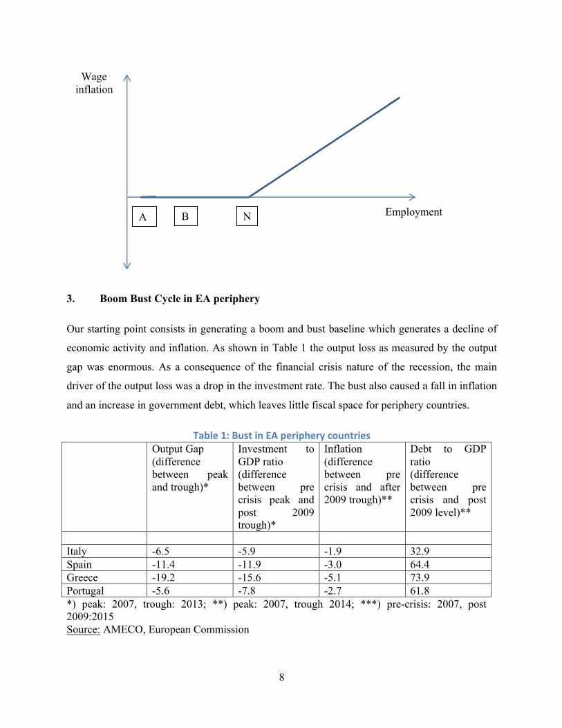
The properties of wage inflation and employment in the presence of a ZBWG are illustrated in

Figure 2. In the inflation employment space we get a positive relationship between wage

inflation and employment. The wage inflation-employment schedule has a kink at point N since

nominal wage growth cannot fall below zero. Suppose the economy is in the constrained regime

with employment level A. Any policy which moves employment up from point A to B will not

be inflationary. Only policies which move employment beyond point N will be inflationary.

Figure2:Wageinflationandemployment

8

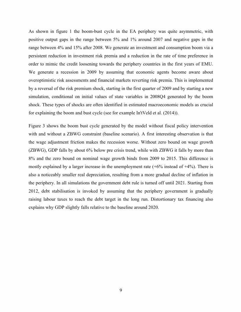
3. Boom Bust Cycle in EA periphery

Our starting point consists in generating a boom and bust baseline which generates a decline of

economic activity and inflation. As shown in Table 1 the output loss as measured by the output

gap was enormous. As a consequence of the financial crisis nature of the recession, the main

driver of the output loss was a drop in the investment rate. The bust also caused a fall in inflation

and an increase in government debt, which leaves little fiscal space for periphery countries.

Table1:BustinEAperipherycountries Output Gap

(difference between peak and trough)*

Investment to GDP ratio (difference between pre crisis peak and post 2009 trough)*

Inflation (difference between pre crisis and after 2009 trough)**

Debt to GDP ratio (difference between pre crisis and post 2009 level)**

Italy -6.5 -5.9 -1.9 32.9 Spain -11.4 -11.9 -3.0 64.4 Greece -19.2 -15.6 -5.1 73.9 Portugal -5.6 -7.8 -2.7 61.8 *) peak: 2007, trough: 2013; **) peak: 2007, trough 2014; ***) pre-crisis: 2007, post 2009:2015 Source: AMECO, European Commission

A N B Employment

Wage inflation

9

As shown in figure 1 the boom-bust cycle in the EA periphery was quite asymmetric, with

positive output gaps in the range between 5% and 1% around 2007 and negative gaps in the

range between 4% and 15% after 2008. We generate an investment and consumption boom via a

persistent reduction in investment risk premia and a reduction in the rate of time preference in

order to mimic the credit loosening towards the periphery countries in the first years of EMU.

We generate a recession in 2009 by assuming that economic agents become aware about

overoptimistic risk assessments and financial markets reverting risk premia. This is implemented

by a reversal of the risk premium shock, starting in the first quarter of 2009 and by starting a new

simulation, conditional on initial values of state variables in 2008Q4 generated by the boom

shock. These types of shocks are often identified in estimated macroeconomic models as crucial

for explaining the boom and bust cycle (see for example In'tVeld et al. (2014)).

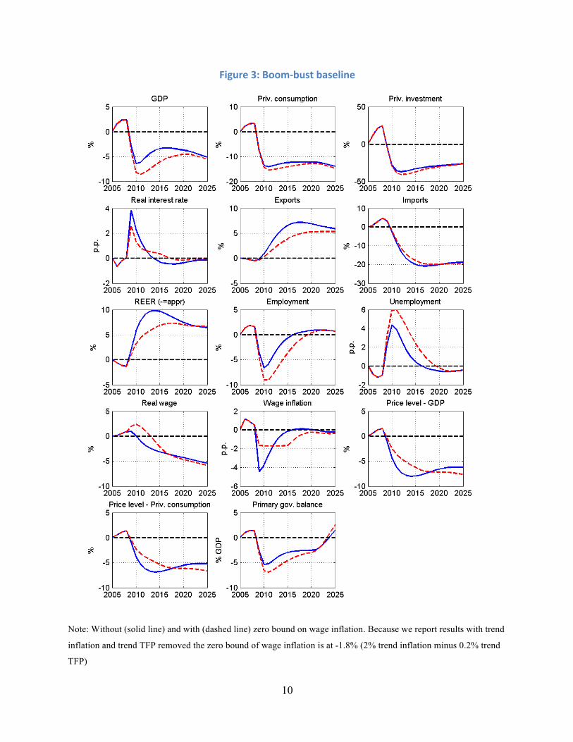
Figure 3 shows the boom bust cycle generated by the model without fiscal policy intervention

with and without a ZBWG constraint (baseline scenario). A first interesting observation is that

the wage adjustment friction makes the recession worse. Without zero bound on wage growth

(ZBWG), GDP falls by about 6% below pre crisis trend, while with ZBWG it falls by more than

8% and the zero bound on nominal wage growth binds from 2009 to 2015. This difference is

mostly explained by a larger increase in the unemployment rate (+6% instead of +4%). There is

also a noticeably smaller real depreciation, resulting from a more gradual decline of inflation in

the periphery. In all simulations the government debt rule is turned off until 2021. Starting from

2012, debt stabilisation is invoked by assuming that the periphery government is gradually

raising labour taxes to reach the debt target in the long run. Distortionary tax financing also

explains why GDP slightly falls relative to the baseline around 2020.

10

Figure3:Boom-bustbaseline

Note: Without (solid line) and with (dashed line) zero bound on wage inflation. Because we report results with trend

inflation and trend TFP removed the zero bound of wage inflation is at -1.8% (2% trend inflation minus 0.2% trend

TFP)

11

4. Fiscal stabilisation: expenditure increase vs. cut in social security contributions

Two alternative fiscal stabilisation strategies can be distinguished, namely an increase in

spending or a reduction in taxation. Advocates of a spending increase point towards the

beneficial effects on the real interest rate if the policy generates some inflation. In a recent paper

Schmitt Grohe and Uribe suggest a temporary wage subsidy as an optimal policy. They argue

that such a policy is directly targeting the labour market inefficiency. In this section we compare

variants of such policies, namely a reduction of social security contributions paid by firms to an

increase in government expenditure. In order to highlight the importance of the ZBWG for the

outcome of fiscal policy we present two alternative cases. We compare the two fiscal strategies

with and without ZBWG.

Case 1: No ZBWG

In order to make both strategies comparable to each other, they both amount to ex ante fiscal

shocks of 1% of GDP over 3 years (gradually phased out). In order to study the degree of self-

financing in the medium term, we assume that the debt stabilisation rule is turned off for 12 years

(until 2021). As can be seen from Figures 4a and 4b, both stabilisation strategies have similar

GDP multipliers of around 0.6. A temporary increase of expenditure crowds out private domestic

demand (inflation effect is positive but small) and worsens the trade balance because of the real

appreciation relative to the rest of the Euro area. In contrast, a reduction of SSC increases

domestic demand (consumption via an increase in real wages and employment and investment

via a reduction in wage costs for firms). Because wage costs and therefore prices decline, there is

a real depreciation which improves the trade balance. Even though prices decline initially the

impact on expected real rate is not very different in both stabilisation strategies. With the

expenditure increase the real rate falls on impact and is expected to increase in the following

years (as prices return to base), while with the SSC reduction, the real interest rate rises initially

but falls in the following years as prices move above base.

Though the overall GDP effects from both strategies is not very different, the distribution across

public private and domestic foreign demand components differs substantially. The expenditure

shock is crowding out private demand and worsens the trade balance, the SSC shock increases

12

private demand and imprioves the trade balance. The latter resembles more closely closely the

composition effect in case the EA periphery would have a monetary policy instrument available.

That both fiscal strategies yield similar GDP effects is of course due to specific elasticities and

should not be seen as a general result. For example, the expansionary effect of an expenditure

based expansion could be higher/smaller if the competitiveness effect was smaller/larger (i. e. a

lower/higher price elasticity of exports and imports)).

13

Figure4a:Fiscalstabilisationviaexpenditureincrease(withoutZBWG)

14

Figure4b:FiscalstabilisationviaSSCreduction(withoutZBWG)

15

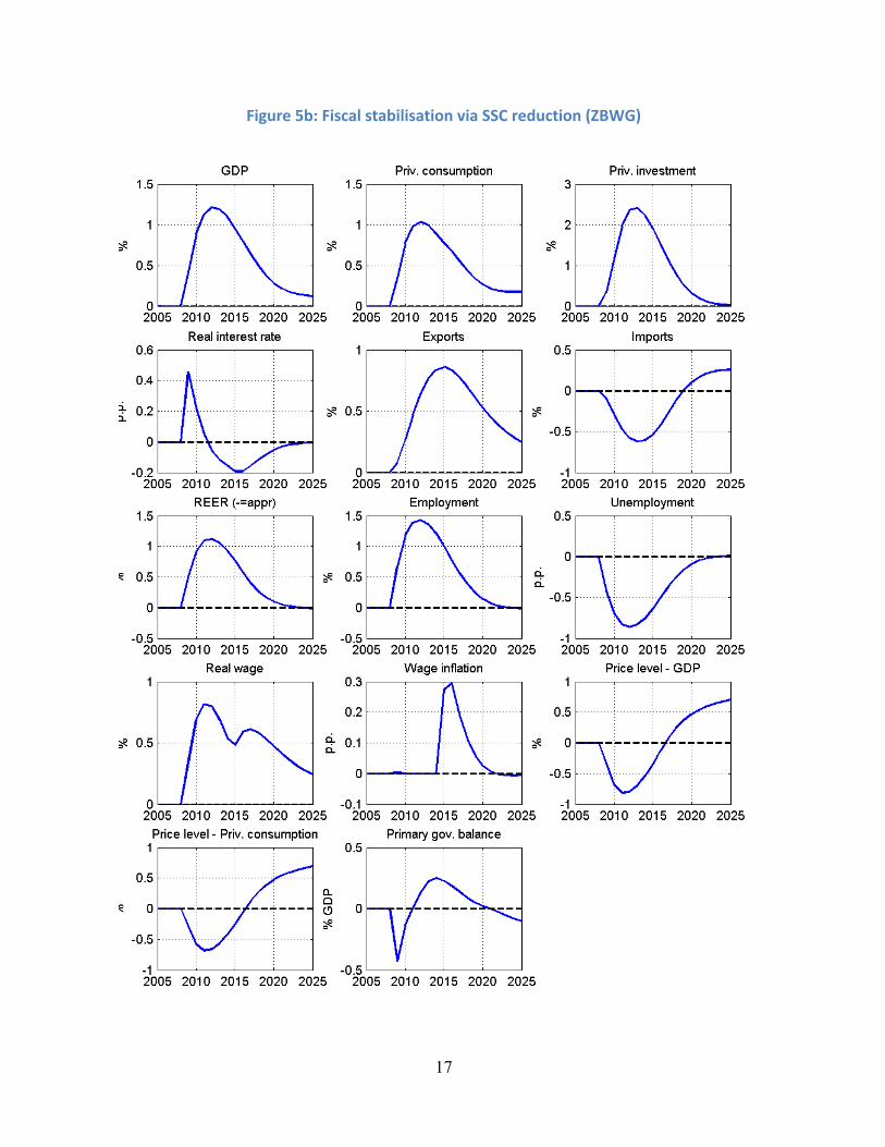
Case 2: With ZBWG

This section shows that the fiscal multiplier of an SSC reduction can be substantially increased in

presence of a binding nominal wage constraint. As can be seen by comparing wage adjustment in

the baseline scenarios (Figure 3), without binding constraint, the nominal wage would decline

more. Therefore, if a fiscal expansion resulting in an increase in labour demand is undertaken in

a constrained wage regime, there is little upward pressure on nominal wages. As a result

(comparing Figure 5b to Figure 4b) the SSC reduction achieves a substantially larger reduction

of wage costs for firms in the constrained wage regime compared to the unconstrained wage

regime. Thus the increase in labour demand is stronger. Even though real wages increase less in

the constrained regime, real wage income increases more because of the positive employment

effect, this increases consumption demand. Also because nominal wage costs fall more, there is a

larger increase of investment. Because prices fall more (stronger decline of wage costs) exports

rise more. This pushes the SSC multiplier above one. Because of the persistent increase of GDP,

consumption and employment (higher labour taxes, lower benefits), the fiscal shock turns out to

be self-financing over the medium term as can be seen from the movement of the primary

balance, with an initial deficit followed by a surplus.

Figure 5a shows that also the public spending multiplier increases under ZBWG, but remains

below 1 (around 0.75). Because of wages being constrained, nominal wage costs initially do not

increase which increases the employment effect of the fiscal expansion, this reduces the

crowding out of private domestic demand. The employment effect thus dominates the real

interest rate effect (smaller decline of the real rate because of lower inflation). However, since

the demand expansion does not directly exploit the fact that nominal wages will remain constant

over a range of increasing demand for labour it is less effective in stabilising the economy than

the SSC reduction. Finally it also appears less efficient in terms of financing properties. Because

of crowding out of domestic demand (in particular consumption) and a smaller increase in

corporate profits, plus a smaller employment effect, public purchases are less tax rich. This

together with the smaller multiplier prevents self-financing of the fiscal measure.

16

Figure5a:Fiscalstabilisationviaexpenditureincrease(ZBWG)

17

Figure5b:FiscalstabilisationviaSSCreduction(ZBWG)

18

Self-financing properties of expenditure increase vs. reduction in social security contributions

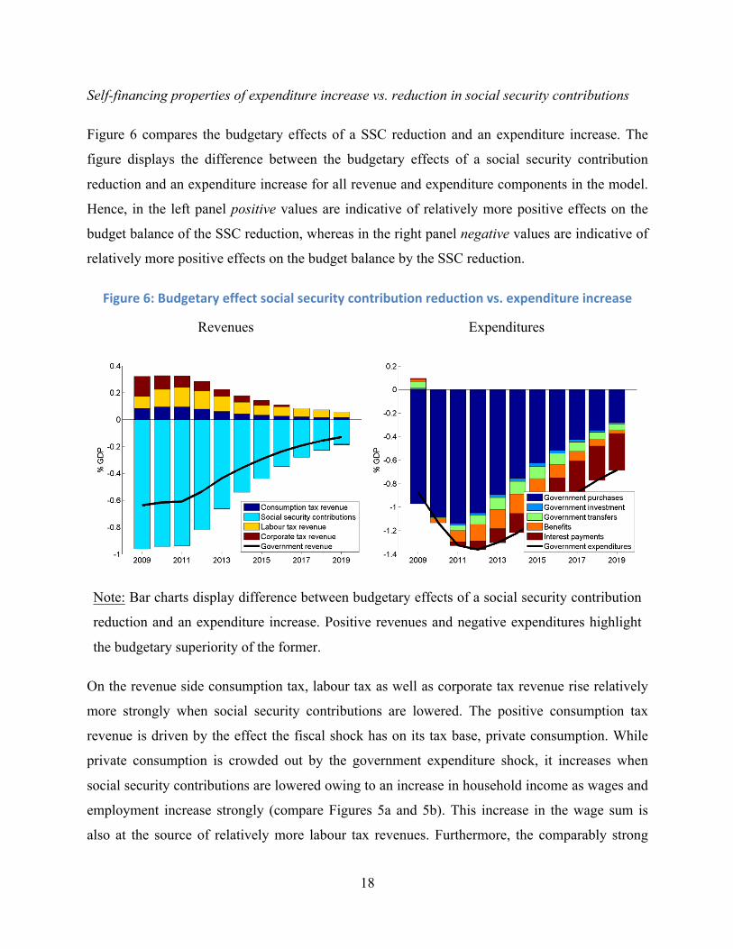
Figure 6 compares the budgetary effects of a SSC reduction and an expenditure increase. The

figure displays the difference between the budgetary effects of a social security contribution

reduction and an expenditure increase for all revenue and expenditure components in the model.

Hence, in the left panel positive values are indicative of relatively more positive effects on the

budget balance of the SSC reduction, whereas in the right panel negative values are indicative of

relatively more positive effects on the budget balance by the SSC reduction.

Figure6:Budgetaryeffectsocialsecuritycontributionreductionvs.expenditureincrease

Revenues Expenditures

Note: Bar charts display difference between budgetary effects of a social security contribution

reduction and an expenditure increase. Positive revenues and negative expenditures highlight

the budgetary superiority of the former.

On the revenue side consumption tax, labour tax as well as corporate tax revenue rise relatively

more strongly when social security contributions are lowered. The positive consumption tax

revenue is driven by the effect the fiscal shock has on its tax base, private consumption. While

private consumption is crowded out by the government expenditure shock, it increases when

social security contributions are lowered owing to an increase in household income as wages and

employment increase strongly (compare Figures 5a and 5b). This increase in the wage sum is

also at the source of relatively more labour tax revenues. Furthermore, the comparably strong

19

increase in the wage sum is causing that social security contribution revenues do not drop one-to-

one with the reduction in its statutory rate. Corporate tax revenues also increase relatively more

strongly as the reduction in social security contributions lowers firm’s costs translating also into

a profit increase. Ex ante the difference in total government revenue in both scenarios is -1% of

GDP by design. Ex post this effect increases to close to -0.6% (solid line in Figure 6, left panel)

in the first year. On the revenue side the reduction in social security contributions is clearly

preferable to an increase in government expenditures.

How the two policies affect the expenditure side depends strongly on the expenditure rules. For

example, if government expenditure is fixed as a share of GDP, then the two policies would have

identical budgetary effects. Here we assume that expenditures (government purchases,

government investment and transfers are fixed in real terms. Therefore there there are two

offsetting effects resulting on the one hand from differences in the size of the GDP effect and on

the other hand from differences in the sign of the real exchange rate effect. Because the SSC

reduction has a larger GDP effect, expenditure as a share of GDP declines more strongly, which

makes the SSC reduction more self-financing. However, this is partly offset by the real

devaluation associated with the SSC reduction, while an expenditure increase leads to real

appreciation. Nevertheless the GDP effect slightly dominates the real exchange rate effect. There

are two additional beneficial effects on the expenditure side. First, because the SSC reduction

reduces unemployment more strongly, unemployment benefit payments are reduced by this

policy. With regards to the relatively stronger negative contribution of interest payments on the

government budget in case of the SSC reduction, it is explained by a significantly smaller

increase in government debt in case of the SSC reduction. Again, ex post the effect on total

government expenditures of the social security contribution reduction is much away from -1%

signalling a comparably stronger self-financing when SSC are reduced compared to when

government expenditures are increased.

5. Conclusion

Boom bust cycles are often characterised by large wage adjustment needs in the bust episode

because of excessive wage growth during the boom, generated by optimistic expectations about

20

future income and employment growth. This is coupled with low demand due to deleveraging

pressures and elevated risk premia in financial markets. These developments can lead to a strong

decline of inflation and generally require a downward adjustment of nominal unit labour costs.

Downward nominal wage rigidities can thus severely slow down the adjustment of the economy.

We find compelling empirical evidence that downward nominal wage rigidity has been a

relevant an adjustment friction in the recent slump episode. Because of wage adjustment

frictions it is often argued (see Uribe et al.) that adjustment in monetary unions can be painful

given the absence of an exchange rate instrument which could move relative prices to their

respective equilibrium levels relatively quickly.

In this paper we compare two fiscal policy strategies for an individual country in EMU which is

hit by a negative demand shock and faces a ZBWG constraint, namely an increase in government

expenditure and reduction in revenues, via a cut in SSC paid by employers. Both fiscal strategies

have been advocated as possible instruments in the current juncture. An expenditure increase can

especially be effective under a ZLB constraint since it raises inflation. A cut in SSC is targeting

the ZBWG constraint and facilitates labour market clearing. It is shown in the paper that for an

open economy in EMU the latter fiscal strategy is superior along two dimensions. First the fiscal

multiplier is larger and the budgetary costs are smaller because the adjustment of the economy to

a SSC reduction is more tax rich. These two features strongly reduce the budgetary cost and

makes this policy measure attractive for a number of periphery countries which suffer from very

limited fiscal space.

References Blanchard, Olivier & Christopher J. Erceg & Jesper Lindé, 2016. "Jump-Starting the Euro Area Recovery: Would a Rise in Core Fiscal Spending Help the Periphery?," NBER Chapters, in: NBER Macroeconomics Annual 2016, Volume 31 National Bureau of Economic Research, Inc. Braun, R. Anton, Lena Mareen Koerber and Yuichiro Waki (2013), "Small and orthodox fiscal multipliers at the zero lower bound," Working Paper 2013-13, Federal Reserve Bank of Atlanta. Christiano, Lawrence & Martin Eichenbaum & Sergio Rebelo, 2011. "When Is the Government Spending Multiplier Large?," Journal of Political Economy, University of Chicago Press, vol. 119(1), pages 78 - 121.

21

Coenen, Günter et al., 2012. "Effects of Fiscal Stimulus in Structural Models," American Economic Journal: Macroeconomics, American Economic Association, vol. 4(1), pages 22-68, January. Elsby, Michael, 2009. "Evaluating the Economic Significance of Downward Nominal Wage Rigidity." Journal of Monetary Economics, 56: 154-69. ECB (2012). "Euro Area Labour Markets and the Crisis," Structural Issues Report. Emmanuel Farhi & Iván Werning, 2014. "Labor Mobility Within Currency Unions," NBER Working Papers 20105, National Bureau of Economic Research, Inc. Holden, Steinar, and Frederik Wulfsberg, 2008. "Downward Nominal Wage Rigidity in the OECD." B.E. Journal Macroeconomics 8:art. 15. In't Veld, J. 2016. "Public Investment Stimulus in Surplus Countries and their Euro Area Spillovers." European Economy - Economic Brief 016. In 't Veld, J., R. Kollmann, B. Pataracchia, M. Ratto, W. Roeger (2014). "International Capital Flows and the Boom-Bust Cycle in Spain". Journal of International Money and Finance pp. 1-22. Linde, J. and M. Trabandt (2016), "Should We Use Linearized Models to Calculate Fiscal Multipliers?" Mimeo. OECD Employment Outlook 2014, "Sharing the Pain equally? Wage Adjustments during the Crisis and Recovery". pp.43-78. Schmitt-Grohe S. and M. Uribe (2016). "Downward nominal wage rigidity, currency pegs and involuntary unemployment. Journal of Political Economy", vol 124, no 5. pp.1466-1514. Uhlig, H. (2016). Discussion of Blanchard, Olivier & Christopher J. Erceg & Jesper Lindé, 2016. NBER Macroeconomics Annual 2016, Volume 31 National Bureau of Economic Research, Inc.

22

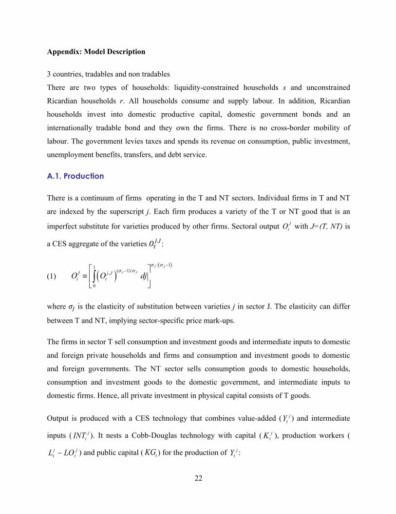
Appendix: Model Description

3 countries, tradables and non tradables

There are two types of households: liquidity-constrained households s and unconstrained

Ricardian households r. All households consume and supply labour. In addition, Ricardian

households invest into domestic productive capital, domestic government bonds and an

internationally tradable bond and they own the firms. There is no cross-border mobility of

labour. The government levies taxes and spends its revenue on consumption, public investment,

unemployment benefits, transfers, and debt service.

A.1. Production

There is a continuum of firms operating in the T and NT sectors. Individual firms in T and NT

are indexed by the superscript j. Each firm produces a variety of the T or NT good that is an

imperfect substitute for varieties produced by other firms. Sectoral output with J=(T, NT) is

a CES aggregate of the varieties 𝑂"h,i:

(1) ( )( )/ 11

( 1)/ ,

0

J J

J JJ j Jt tO O dj

s ss s

--é ù

º ê úë ûò

where 𝜎i is the elasticity of substitution between varieties j in sector J. The elasticity can differ

between T and NT, implying sector-specific price mark-ups.

The firms in sector T sell consumption and investment goods and intermediate inputs to domestic

and foreign private households and firms and consumption and investment goods to domestic

and foreign governments. The NT sector sells consumption goods to domestic households,

consumption and investment goods to the domestic government, and intermediate inputs to

domestic firms. Hence, all private investment in physical capital consists of T goods.

Output is produced with a CES technology that combines value-added ( ) and intermediate

inputs ( ). It nests a Cobb-Douglas technology with capital ( ), production workers (

) and public capital ( ) for the production of :

JtO

jtY

jtINT j

tKjt

jt LOL - tKG j

tY

23

(2) ( ) ( ) ( ) ( )/( 1)1 1( 1)/ ( 1)/

1in in

in in in inin in

j j j j jt in t in tO s Y s INT

s ss s s s

s s

-- -é ù

= - +ê úë û

(3)

where jins and are, respectively, the share parameter of intermediates in output and the

elasticity of substitution between intermediates and value-added, and , , and

are total factor productivity (TFP), capacity utilisation, overhead labour and fixed costs of

producing.1

Firm-level employment is a CES aggregate of variants of labour services:

(4) 𝐿"h = 𝐿"

h(𝑖)lI8l 𝑑𝑖'

n

llI8with 𝜃 > 1

where indicates the degree of substitutability between the different types of labour i.

The firm hires workers, rents capital and buys intermediate inputs. The demand for inputs and

pricing decisions result from profit ( ) maximisation subject to adjustment costs for changing

prices (𝑎𝑑𝑗"P,h), employment (𝑎𝑑𝑗"

),h) and capacity (𝑎𝑑𝑗"qrst,h):

(6) ( ) ( ), , , ,1j j j INT j j J j J I j P j L j ucap jt t t t t t t t t t t t t tPr p O p INT ssc wL i p K adj adj adj= - - + - - + +

where , , and are the employer social security contributions, the real wage, the

rental rate of capital, and the price of capital. Adjustment costs are quadratic:

(7a)

(7b) with

1 Lower case letters denote ratios and rates. In particular, /j j

t t tp P Pº is the price of good j relative to the GDP deflator, /t t tw W Pº is the real

wage, jtucap is actual relative to steady-state (full) capital utilisation, and

te is the nominal exchange rate defined as the price of foreign in

domestic currency.

1( ) ( ) gj j j j j j jt t t t t t t tY A ucap K L LO KG FCYaa a-= - -

ins

jtA

jtucap j

tLOjtFCY

jtL

q

Pr jt

Jtssc tw J

tiItp

, 2( ) / 2L j jt L t tadj w Lgº D

, 2( ) / 2P j j jt P t tadj Yg pº 1 1j j j

t t tP Pp -º -

24

(7c)

A.2. Households

The household sector consists of a continuum of households [ ]1,0Îh . There are 1£ls

households which are liquidity-constrained and indexed by l. These households do not trade on

asset markets and consume their disposable income each period. A fraction rs of all households

are Ricardian and indexed by r. The period utility function is identical for Ricardian and

liquidity-constrained households and separable in consumption ( htC ), and leisure ( h

tL-1 ). We

also allow for habit persistence in consumption ( ch ).

(8)𝑈 𝐶", 𝐿"(𝑖) = 𝛽" log 𝐶" − ℎr𝐶"(' + w'(x

(1 − 𝐿(𝑖)"𝑑𝑖)'n

'(xy"zn

The two types of households supply differentiated labour services to unions which maximise a

joint utility function for each type of labour i on behalf of households. It is assumed that types of

labour are distributed equally over the two household types. Nominal rigidity in wage setting is

introduced by assuming that the household faces adjustment costs for changing wages. These

adjustment costs are borne by the household.

A.2.1. Ricardian households

Ricardian households have full access to financial markets. They hold domestic government

bonds (𝐵"|) and bonds issued by other domestic and foreign households ( rFt

rt BB ,, ), real capitals

( jtK ) of the tradable and non-tradable sector. The household receives income from labour (net

of adjustment costs on wages), financial assets, rental income from lending capital to firms, plus

profit income from firms owned by the household (tradables, non-tradables, and residential

construction). The unemployed (1-npart-L) receive benefits ben, while in addition there is

income from general transfers TR. Income from labour is taxed at rate tw. We allow for taxes on

corporate profits, tk. Finally, households pay lump-sum taxes TLS. Domestic bonds yield risk-free

nominal return equal to it. Foreign bonds are subject to (stochastic) risk premia linked to net

foreign indebtedness.

, 2,1 ,2[ ( 1) ( 1) ] / 2ucap j I j j j

t t t ucap t ucap tadj p K ucap ucapg gº - + -

25

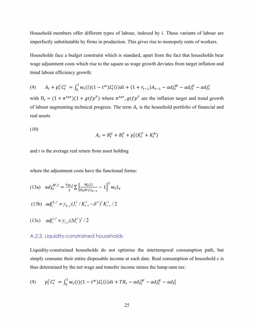
Household members offer different types of labour, indexed by 𝑖. These variants of labour are

imperfectly substitutable by firms in production. This gives rise to monopoly rents of workers.

Households face a budget constraint which is standard, apart from the fact that households bear

wage adjustment costs which rise to the square as wage growth deviates from target inflation and

trend labour efficiency growth:

(9) 𝐴" + 𝑝"%𝐶"~ = 𝑤"(𝑖)(1 − 𝑡1)𝐿"~ 𝑖 𝑑𝑖'n + 1 + 𝑟"(' 𝐴"(' − 𝑎𝑑𝑗"O − 𝑎𝑑𝑗"� − 𝑎𝑑𝑗"�

with Π� = (1 + 𝜋"s~)(1 + 𝑔𝑡𝑓𝑝�) where 𝜋"s~, 𝑔𝑡𝑓𝑝� are the inflation target and trend growth

of labour augmenting technical progress. The term 𝐴" is the household portfolio of financial and

real assets

(10) 𝐴" = 𝐵"| + 𝐵"� + 𝑝"�(𝐾"� + 𝐾"�)

and r is the average real return from asset holding

where the adjustment costs have the functional forms:

(13a) 𝑎𝑑𝑗"O,i = <�,�

�O* +

�*O(+)*I8− 1

�𝑤"𝐿"

(13b)

(13c)

A.2.3. Liquidity-constrained households

Liquidity-constrained households do not optimise the intertemporal consumption path, but

simply consume their entire disposable income at each date. Real consumption of household c is

thus determined by the net wage and transfer income minus the lump-sum tax:

(9) 𝑝"%𝐶"~ = 𝑤"(𝑖)(1 − 𝑡1)𝐿"~ 𝑖 𝑑𝑖'n + 𝑇𝑅" − 𝑎𝑑𝑗"O − 𝑎𝑑𝑗"� − 𝑎𝑑𝑗"�

, 2, 1 1( / ) / 2K J J J J J

t K J t t tadj I K Kg d- -º -

, 2, ( ) / 2I J J

t I J tadj Igº D

26

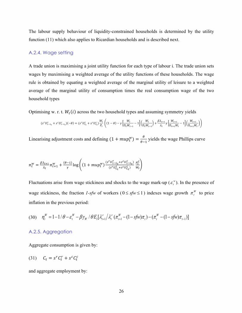
The labour supply behaviour of liquidity-constrained households is determined by the utility

function (11) which also applies to Ricardian households and is described next.

A.2.4. Wage setting

A trade union is maximising a joint utility function for each type of labour i. The trade union sets

wages by maximising a weighted average of the utility functions of these households. The wage

rule is obtained by equating a weighted average of the marginal utility of leisure to a weighted

average of the marginal utility of consumption times the real consumption wage of the two

household types

Optimising w. r. t. 𝑊" 𝑖 across the two household types and assuming symmetry yields

(𝑠~𝑈'()*~ + 𝑠r𝑈'()*

r ) −𝜃 = (𝑠~𝑈%*~ + 𝑠r𝑈%*

r )𝑊"

𝑃" 1 − 𝜃 − 𝛾

𝑊"

Π"𝑊"('− 1

𝑊"

Π"𝑊"('+𝛽𝜆".'𝜆"

𝛾𝑊".'

Π".'𝑊"− 1

𝑊".'

Π".'𝑊"

Linearising adjustment costs and defining (1 + 𝑚𝑢𝑝"1) =;

;(' yields the wage Phillips curve

𝜋"1 = 56*786*

𝜋".'1 + ;('<

log 1 + 𝑚𝑢𝑝"1(FGH8IJ*

G .FKH8IJ*K )

(FGHM*G .FKHM*

K )P*

M

O*

Fluctuations arise from wage stickiness and shocks to the wage mark-up ( ). In the presence of

wage stickiness, the fraction 1-sfw of workers ( ) indexes wage growth to price

inflation in the previous period:

(30) 1 1 11 1/ / [ ( (1 ) ) ( (1 ) )]W W r r W Wt t W t t t t t t tE sfw sfwh q e bg q l l p p p p+ + -= - - - - - - - -

A.2.5. Aggregation

Aggregate consumption is given by:

(31) 𝐶" = 𝑠~𝐶"~ + 𝑠r𝐶"r

and aggregate employment by:

wte

10 ££ sfw Wtp

27

(32) 𝐿" = 𝑠~𝐿"~ + 𝑠r𝐿"r with𝐿"~ = 𝐿"r .

A.3. Fiscal and monetary policy

We assume that except for explicit discretionary interventions, governments keep consumption

and investment constant in real terms. Thus nominal government purchases ( ) and investment

(𝐼"|) are kept constant in real terms.

(33) 𝐺" = 𝑔𝑝"%

(34) 𝐼"| = 𝚤|𝑝"%

Also the real consumption value of transfers are kept constant ( )

(35) 𝑇𝑅" = 𝑡𝑟𝑝"%

The nominal benefits paid to the non-employed part of the labour force correspond to the

exogenous replacement rate (𝑏𝑒𝑛) times the nominal wage:

(36) 𝐵𝐸𝑁" = 𝑏𝑒𝑛𝑤"(𝐿" − 𝐿𝐹")

The government receives consumption tax, labour tax, corporate tax and lump-sum tax revenue

as well as social security contributions. Nominal government debt ( ) evolves according to:

(37) 𝐵" = 1 + 𝑖"(' 𝐵"(' + 𝐺" + 𝐼"| + 𝑇𝑅" + 𝐵𝐸𝑁" − 𝑇")� − 𝑡"%𝑃"%𝐶" − 𝑡"O + 𝑠𝑠𝑐" 𝑊"𝐿" − 𝑡"�𝑃𝑅"

Labour taxes are used to stabilise the debt-to-GDP ratio:

(38) ∆𝑡"O = 𝜏� �P*�*

− 𝑏 + 𝜏 ∆𝐵"

with b being the target government debt to GDP ratio. The consumption tax, corporate income

tax and personal income tax rates and the rate of social security contributions are exogenous.

Monetary policy follows a Taylor rule that allows for a smoothing of the interest rate response to

inflation and the output gap:

tG

tTR

tB

28

(39)

The central bank has an inflation target , adjusts its policy rate when actual CPI inflation

deviates from the target and also responds to the output gap (ygap). The output gap is not

calculated as the difference between actual and efficient output, but derived from a production

function framework, which is the standard practice of output gap calculation for fiscal

surveillance and monetary policy. More precisely, the output gap is defined as deviation of factor

utilisation from its long-run trend:

(40)

The variables and are moving averages of employment and capacity utilisation rates:

(41a)

(41b)

The moving averages are restricted to move slowly in response to actual values.

A.4 Trade and financial linkages

In order to facilitate aggregation, private households and the government are assumed to have

identical CES preferences across goods used for consumption and investment. (42)

( ) ( ) ( ) ( )/( 1)1/ ( 1)/ 1/ ( 1)/

1tnt tnt

tnt tnt tnt tnt tnt tntT NT T Tt t tZ s Z s Z

s ss s s s s s -- -é ù= - +ê úë û

where 𝑍"𝜖 𝐶", 𝐺", 𝐼"�, 𝐼"�, 𝐼"| and NTtZ and 𝑍"�is an index of demand across the NT and T

varieties. Concerning, 𝑍"� households and the government have identical CES preferences

regarding domestically produced and imported goods ( ,T DtZ ) and ( ,T M

tZ ) respectively:

(43) ( ) ( )/( 1)( 1)/ ( 1)/1/ 1/, ,(1 )x x

x x x xx xT T D T M

t m t m tZ s Z s Zs ss s s ss s

-- -é ù= - +ê úë û

( )1 (1 ) ( )tar C tart i t i t y ti i r ygappr r p t p p t-= + - + + - +

tarp

ln( / ) (1 ) ln( / )ss sst t t t tygap L L ucap ucapa aº + -

sstL

sstucap

1 (1 )ss L ss Lt t tL L Lr r-= + -

1 (1 )ss ucap ss ucap jt t tucap ucap ucapr r-= + -

29

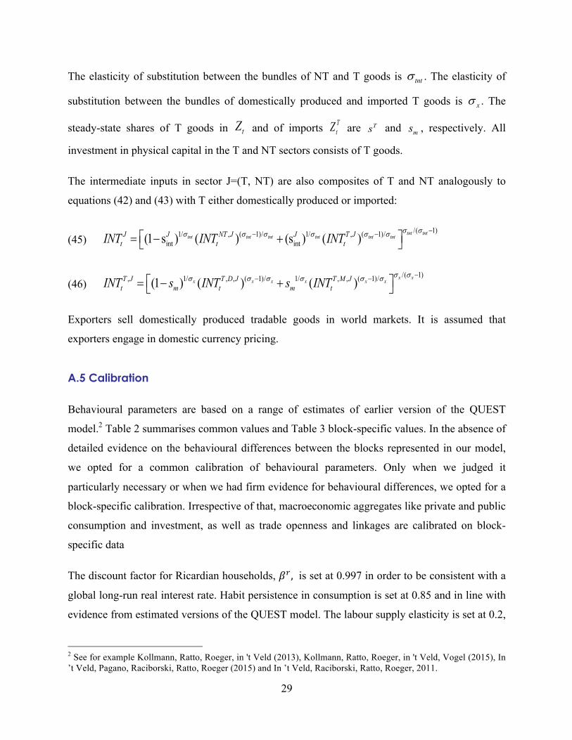
The elasticity of substitution between the bundles of NT and T goods is . The elasticity of

substitution between the bundles of domestically produced and imported T goods is . The

steady-state shares of T goods in tZ and of imports TtZ are Ts and , respectively. All

investment in physical capital in the T and NT sectors consists of T goods.

The intermediate inputs in sector J=(T, NT) are also composites of T and NT analogously to

equations (42) and (43) with T either domestically produced or imported:

(45) /( 1)1/ ( 1)/ 1/ ( 1)/, ,

int int(1 s ) ( ) (s ) ( ) tnt tnttnt tnt tnt tnt tnt tntJ J NT J J T J

t t tINT INT INTs ss s s s s s -- -é ù= - +ë û

(46) /( 1)1/ ( 1)/ 1/ ( 1)/, , , , ,(1 ) ( ) ( ) x x

x x x x x xT J T D J T M Jt m t m tINT s INT s INT

s ss s s s s s -- -é ù= - +ë û

Exporters sell domestically produced tradable goods in world markets. It is assumed that

exporters engage in domestic currency pricing.

A.5 Calibration

Behavioural parameters are based on a range of estimates of earlier version of the QUEST

model.2 Table 2 summarises common values and Table 3 block-specific values. In the absence of

detailed evidence on the behavioural differences between the blocks represented in our model,

we opted for a common calibration of behavioural parameters. Only when we judged it

particularly necessary or when we had firm evidence for behavioural differences, we opted for a

block-specific calibration. Irrespective of that, macroeconomic aggregates like private and public

consumption and investment, as well as trade openness and linkages are calibrated on block-

specific data

The discount factor for Ricardian households, 𝛽~, is set at 0.997 in order to be consistent with a

global long-run real interest rate. Habit persistence in consumption is set at 0.85 and in line with

evidence from estimated versions of the QUEST model. The labour supply elasticity is set at 0.2,

2 See for example Kollmann, Ratto, Roeger, in 't Veld (2013), Kollmann, Ratto, Roeger, in 't Veld, Vogel (2015), In ’t Veld, Pagano, Raciborski, Ratto, Roeger (2015) and In ’t Veld, Raciborski, Ratto, Roeger, 2011.

tnts

xs

ms

30

which lies at the lower end of the range of estimation results from the QUEST model. This is in

line with evidence from Chetty (2012). Concerning adjustment costs on labour, goods and capital

we broadly follow earlier estimations of the QUEST model. The shares of forward looking wage

and price setters, 𝑠𝑓𝑝 and 𝑠𝑓𝑤, is calibrated to 0.9 reflecting the extent to which agents base

their decisions on model consistent expectations. The elasticity of substitution between tradables

and non-tradables 𝜎"£" is set following evidence from the IMF's GIMF model (see Kumhof et al.,

2010).

The output elasticity for public capital 𝛼¥is set at 0.09, such that the marginal product of public

capital equates that of private capital (Gramlich, 1994). Setting the elasticity of substitution

between types of labour, 𝜃, at 6 induces a wage mark-up of 20%. Tax rule parameters 𝜏¦ and

𝜏 §¨ are chosen to assure a smooth transition to the long-run debt target. In setting the reaction

coefficient to inflation in the Taylor rule, 𝜏©, at 2 we closely follow the literature.

Table 2: Calibration – common values

Parameter Value Description 𝛽~ 0.997 Discount factor Ricardian households ℎr 0.85 Habit persistence in consumption 1/𝜅 0.2 Labour supply elasticity 𝛾) 25 Head-count adjustment costs parameter 𝛾P 20 Price adjustment costs parameter

𝛾qrst,' 0.04(T) 0.03(NT) Linear capacity-utilisation adjustment cost

𝛾qrst,� 0.05 Quadratic capacity-utilisation adjustment cost 𝛾� 20 Capital adjustment cost 𝛾� 75 Investment adjustment cost 𝛾O 120 Wage adjustment cost 𝛾« 40 Adjustment costs to the housing stock 𝑠𝑓𝑝 0.9 Share of forward looking price setters 𝛾¬ 5 Adjustment cost parameter export prices 𝑠𝑓𝑤 0.9 Share of forward looking wage setters 𝜎"£" 0.5 Elasticity of substitution T-NT 𝜎­ 1.2 Elasticity of substitution in total trade 𝜎 0.99 Elasticity of substitution between import sources 𝛼 0.65 Cobb-Douglas labour parameter 𝛼¥ 0.09 Cobb-Douglas public capital stock parameter 𝜎+£ 0.5 Elasticity of substitution between value added and intermediates 𝜃 6 Elasticity of substitution between types of labour 𝛿� 0.015 Depreciation rate T capital stock 𝛿�� 0.005 Depreciation rate NT capital stock 𝛿¥ 0.013 Depreciation rate public capital stock 𝜌) 0.95 Persistence of potential employment

𝜌qrst 0.99 Potential capacity utilisation persistence 𝜏¦ 0.01 Tax rule parameter on debt 𝜏 §¨ 0.1 Tax rule parameter on deficit 𝜌+ 0.6 Interest rate smoothing in Taylor rule

31

Parameter Value Description 𝜏© 2 Reaction coefficient to inflation in Taylor rule

Table 3 features block-specific values of the calibration. Concerning financial market frictions in

advanced economies, we assume 60 percent of households to have full access to financial

markets, which corresponds closely to our estimates (Ratto et al., 2009). Labour force to total

population and employment shares are taken from national sources and are aggregated for the

corresponding block. Steady-state consumption shares of imports, the share of intermediates in

the tradable and non-tradable sector are based on input-output tables from the GTAP database

(see Narayanan and Walmsley, 2008). The share of bilateral imports are compiled from the

direction of trade statistics provided by the IMF and aggregated netting out intra-block. The

baseline debt-to-GDP ratio is based on an average debt-to-GDP ratios observed over the last 5 to

10 years. The mildly higher reaction coefficient to output in the Taylor rule of the US compared

to other regions is motivated by the mandate of the Federal Reserve which suggests a relatively

stronger focus on economic activity.

Table 3: Calibration - block-specific values

Parameter Value Description EA Periphery

EA Core

RoW

𝑠~ 0.6 0.6 0.6 Share of Ricardian households 𝑠° 0.4 0.4 0.4 Share of liquidity-constrained households

1 − 𝑛𝑝𝑎𝑟𝑡 0.71 0.71 0.71 Labour force to population 𝐿 0.64 0.64 0.70 Steady state employment to population

1/𝜎�

0.12 0.12 0.12 Mark-up T sector

1/𝜎�� 0.24 0.24 0.2 Mark-up NT sector 𝑠� 0.4 0.4 0.3 Steady-state share of T 𝑠± 0.22 0.33 0.24 Steady-state consumption share of imports 𝑠+£� 0.73 0.76 0.62 Steady-state share of intermediates in

output T 𝑠+£�� 0.50 0.59 0.45 Steady-state share of intermediates in

output NT

𝑠+£"� 0.67 0.61 0.72 Steady-state T intermediate share in T

𝑠+£"�� 0.47 0.43 0.44 Steady-state T intermediate share in NT

𝑠²³(P,¨ - Share of bilateral imports of EA periphery 𝑠²³(%,¨ - Share of bilateral imports of EA core 𝑠´µ1,¨ - Share of bilateral imports of RoW 𝑏𝑡𝑎𝑟 0.8 0.7 0.8 Baseline government debt-to-GDP ratio 𝜏¶ 0.1 0.1 0.15 Reaction coefficient to output gap in Taylor

rule

32

Figure7:Wages,unemploymentrateandGDPinselectedEAcountries

Labour cost index, business economy

(2008=100)

Unemployment rate (absolute deviation from

2008 value)

Real GDP (2008=100)

Source: Eurostat (LCI), AMECO (other variables)

5060708090

100110120

1999

2002

2005

2008

2011

2014

-5

0

5

10

15

20

1999

2002

2005

2008

2011

2014

70

80

90

100

1999

2002

2005

2008

2011

2014

EL

ES

IT

CY

PT

SI