Embed Size (px)
Citation preview


ISSN 1518-3548 CGC 00.038.166/0001-05
Working Paper Series Brasília n. 240 Apr. 2011 p. 1-81

Working Paper Series Edited by Research Department (Depep) – E-mail: [email protected] Editor: Benjamin Miranda Tabak – E-mail: [email protected] Editorial Assistant: Jane Sofia Moita – E-mail: [email protected] Head of Research Department: Adriana Soares Sales – E-mail: [email protected] The Banco Central do Brasil Working Papers are all evaluated in double blind referee process. Reproduction is permitted only if source is stated as follows: Working Paper n. 240. Authorized by Carlos Hamilton Vasconcelos Araújo, Deputy Governor for Economic Policy. General Control of Publications Banco Central do Brasil
Secre/Surel/Cogiv
SBS – Quadra 3 – Bloco B – Edifício-Sede – 1º andar
Caixa Postal 8.670
70074-900 Brasília – DF – Brazil
Phones: +55 (61) 3414-3710 and 3414-3565
Fax: +55 (61) 3414-3626
E-mail: [email protected]
The views expressed in this work are those of the authors and do not necessarily reflect those of the Banco Central or its members. Although these Working Papers often represent preliminary work, citation of source is required when used or reproduced. As opiniões expressas neste trabalho são exclusivamente do(s) autor(es) e não refletem, necessariamente, a visão do Banco Central do Brasil. Ainda que este artigo represente trabalho preliminar, é requerida a citação da fonte, mesmo quando reproduzido parcialmente. Consumer Complaints and Public Enquiries Center Banco Central do Brasil
Secre/Surel/Diate
SBS – Quadra 3 – Bloco B – Edifício-Sede – 2º subsolo
70074-900 Brasília – DF – Brazil
Fax: +55 (61) 3414-2553
Internet: http://www.bcb.gov.br/?english
3
Fiscal Policy in Brazil through the Lens
of an Estimated DSGE model**
Fabia A. de Carvalho *** Marcos Valli ****
Abstract
This paper takes Brazilian data to an open economy DSGE model that features realistic aspects of fiscal policy in Brazil. The model incorporates primary surplus targets, cyclical expenditures and social programs in the form of public transfers, public investment and distortive taxation. We test for two competing specifications of the role of public capital in the real economy. Bayesian model comparison favors the infrastructure approach to public capital. The presence of non-Ricardian households allows fiscal policy shocks to affect real economy aggregates and distribution. The model is used to address questions regarding the effect of shocks to different fiscal policy instruments upon the business cycle. We also investigate whether recent fiscal policy in Brazil has exerted significant inflationary pressures. Keywords: DSGE, fiscal policy, monetary policy, government investment, public capital, primary surplus, heterogeneous agents, market frictions, Bayesian estimation JEL Classification: E32; E62; E63
* We are thankful to Michel Juillard for important comments and suggestions, and to the participants of
the 32nd Meeting of the Brazilian Econometric Society. ** Research Department, Banco Central do Brasil. *** Department of Banking Operations and Payments System, Banco Central do Brasil.
The Working Papers should not be reported as representing the views of the Banco Central do Brasil. The views expressed in the papers are those of the author(s) and not
necessarily reflect those of the Banco Central do Brasil.

4
1 Introduction
The recent global financial crisis has brought fiscal policy back into spotlight. Facing
major recession outlooks and approaching the zero lower bound of interest rates,
developed economies have put forth significant fiscal stimuli as an attempt to boost
economic recovery. In emerging markets, fiscal policy stimuli were also promptly set
up to fight the recessionary risks of the crisis. In the specific case of Brazil, although the
crisis abated much quicker than in developed economies (Figure 1), fiscal stimuli have
not been completely withdrawn (Figure 2).
For some time now there has been a local debate on whether and to what extent the
recent expansionary stance of Brazilian fiscal policy, put in place during the recent
crisis, could jeopardize the achievement of inflation targets. Advocates in favor of fiscal
interventions often argue that not all the adopted fiscal measures are inflationary; public
investments, for instance, could be favorable to balanced growth through the supply
side. Notwithstanding, the local debate still lacks an analytical tool that can properly
account for the intricate economic responses of both fiscal and monetary policies
in action.
This paper explores one possible tool for the analysis of fiscal and monetary policy in
Brazil. We adapt a state-of-the-art open economy DGSE model to account for a more
realistic setting of the fiscal policy from the standpoint of policy practice in Brazil. We
bring the model to Brazilian data to investigate the dynamic responses of the economy
to fiscal policy shocks and the effects of their interaction with monetary policy. The
main questions we address are: 1) how does the type of fiscal expenditure matter for the
business cycle?; 2) to what extent can an expansionist shock to the primary surplus put
the accomplishment of central bank’s inflation target at risk?; and 3) has the conduct of
fiscal policy in Brazil in recent years put pressure on inflation?
The fiscal setting of the model departs from the tradition in the DSGE literature of
addressing fiscal policy exclusively through lump sum taxes/transfers and a mean-
reverting rule for current government expenditures. First, we introduce a state-
dependent (net-of-interest) primary balance rule. With the implementation of an IMF

5
agreement back in 1998, Brazil committed to a primary surplus target that was intended
to drive public debt to more sustainable levels in the long run. The target was to be
complied with on a quarterly basis. The IMF agreement was renewed in 2001, amid a
series of external and domestic shocks, including an energy shortage, and was extended
and augmented in 2003.
In December 2005, the Brazilian government made an early full repayment of the
outstanding debt with the IMF. Such an act also implied that the targets set forth in the
IMF agreement would cease to be enforced. Notwithstanding, the government
understood that the market factored in a commitment to a debt-reducing primary surplus
target as a good sign of sound fiscal management, thus improving sovereign credit
ratings and alleviating the burden of new issuances of public debt. The Brazilian
government then decided to keep on announcing primary surplus targets for the fiscal
years, and in general enforced an anti-cyclic budget execution.
The DSGE literature has experimented with some non-trivial state-dependent fiscal
rules. In most cases, the preferred specification is based on rules for current government
expenditures or taxes that respond to output and to debt1. In practice, a government with
targets for the primary balance makes concomitant decisions on all sorts of
expenditures, revenues, transfers, subsidies, tax recovery and exemptions. The identified
shocks to the primary surplus rule in our model are thus a summary measure of changes
in policymakers’ preferences.
The second adaptation we introduce in our model is to let the government intervene in
the economy through the accumulation of public capital, with an impact on factor
productivity and in the overall demand for investment goods.
1 Medina and Soto (2007) analyze three types of fiscal rules: one where government expenditures adjust to satisfy government’s budget constraint, another where government taxes do such as task, and the last one where government expenditures as a share of GDP adjust to meet a target for the “structural” balance, measured as the nominal fiscal result adjusted for cyclical revenues from government’s budget flow. Forni et. al. (2009) use tax rules that react to the debt-to-GDP ratio, and report that expenditure rules yield similar impact of the fiscal shocks to the economy. In CMS, lump-sum taxes are the chosen instrument to stabilize the debt-to-GDP ratio. Ratto et. al. (2009) introduce a rule for public investment that responds to the business cycle.

6
We test for two competing specifications of the way public capital affects factor
productivity in Brazil. In the first specification, which draws from the work of Ratto et.
al. (2009), we let public capital augment factor productivity at no direct cost for the
firm. Public capital in this case can be interpreted as an externality to the private
productive sector. As Macdonald (2008) points out, this is the most standard way of
estimating production functions in economies with relevant public infrastructure, but it
misses the important point that such expenditures are financed by society, and
sometimes financing can be directly associated with the economic activity that is more
intense on the use of such public capital goods. In our specification, financing of public
capital is indirect, through the general tax system, and is not factored into the cost
accounting of firms.
In the second specification of the role of public capital in the economy, we assume that
the costs associated with the use of public capital are born by its direct users, the
intermediate goods firms. We also assume that, to a certain extent, firms can selectively
choose between public and private capital services. This modeling choice was intended
to capture the significant presence of the Brazilian government in the productive sector
of the economy. In spite of a vast number of privatizations carried out over the past
decades, Brazil still has a substantial number of mixed-capital firms (118 federal
enterprises, as of January 2010) on top of high and increasing public loans to finance
private capital2. Some of these loans are extended with guarantees in the form of
ownership transfers of funded capital to the government. Although this type of capital
belongs to the government, it does not possess the characteristics of a public good: it is
employed uniquely at the production of the individual firm and does not produce
externalities to the other firms of the economy.
To allow fiscal policy to have an effect on aggregate consumption, we follow Coenen,
McAdam and Straub (2008), hereinafter referred to as CMS, and introduce non-
Ricardian agents in the model.3 These agents are optimizing consumers, but, in addition
to being constrained on their access to capital markets and investment choices, non- 2 As of October 2010, total outstanding loans extended by public financial institutions amounted to 19.8% of GDP. 3 Although the 59% of non-Ricardian agents calibrated for the domestic economy is higher than the 25% calibrated for the Euro Area, it is close to the 50% used in Galí et. al. (2004), and is substantially lower than the 70% considered for Chile in Medina and Soto (2007).

7
Ricardian agents in our model are less productive than the other group of agents. This
assumption is necessary to allow for a steady state where different groups of workers
can work the same amount of hours but earning different wages.
The fourth novelty in our fiscal setup is the introduction of social programs in the form
of transfers to the worse-off. For the past years, these programs have gained a lot of
importance in the Brazilian policy agenda. The most popular program, “Bolsa Família”,
has consisted of monthly transfers of public funds to about 11 million households
in Brazil.
The rest of the model follows the essence of the calibrated version of ECB’s New Area
Wide Model presented in CMS. In addition to the changes we introduce in the fiscal
setup and the assumption of labor heterogeneity, we modify the final goods price index
and the recursive representation of wage setting decision rules and wage dispersion
index4, and introduce risk premia in the negotiation of foreign and domestic debt, the
former playing an active role even in the steady state so as to account for the fact that
real interest rates in Brazil are substantially higher than in the developed world. As in
the estimated version of ECB’s NAWM presented in Christoffel, Coenen and Warne
(2008), hereinafter referred to as CCW, our model features trending growth in
labor productivity.
We estimate the model using Bayesian methods. The data density favors the model that
specifies public capital as an externality to firms. We use this model as benchmark to
produce Bayesian impulse responses to the shocks in the model. From the IRFs, we
show that: 1) the type of fiscal expenditures greatly matters for the business cycle; 2)
fiscal shocks are usually inflationary; 3) fiscal policy preferences have not been
identified as important drivers of the recent path of consumer inflation in Brazil; but 4)
fiscal policy preferences have played an important role in the historical execution of the
primary surplus.
In addition, we conduct policy exercises and show that greater reaction of fiscal policy
to deviations of public debt or GDP growth from their steady states can significantly
4 The details on the theoretical revisions can be found in Valli and Carvalho (2010).

8
destabilize the model’s dynamics. On the other hand, stronger reaction of the monetary
authority to output growth produces muter responses to inflation and output after
monetary policy shocks.
Motivated by the policy debate about the possibility of reducing the primary surplus
target in Brazil, we analyze the model’s dynamics under a drastic reduction in the target.
We show that this would not enact significant changes in the dynamic responses of real
and nominal variables of the model; however, and quite importantly, such a reduction in
the target can only be accomplished if the ratio of public debt to GDP is also sharply cut
down. Otherwise, the economy can undergo explosive paths.
Our simulations also show that the presence of non-Ricardian agents has important
implications for the responses of real variables to fiscal policy shocks, notwithstanding
the fact that our non-Ricardian agents are intertemporal optimizers, yet with more
restraints than the Ricardians.
The paper is organized as follows. Section 2 provides an overview of the model. Section
3 details the estimation procedure, reporting on the strategy for calibrating the steady
state of the model, the reasons underlying the choices of priors, and also describing the
data and the shocks. Section 4 analyses the impulse responses of the model and presents
the historical decomposition of some key macroeconomic variables. Section 5 reports
on some policy exercises. The last section concludes the paper.
2 The model
Figure 3 depicts the core structure of the model. The model is composed of two
economies of different sizes that interact in goods and financial markets. The foreign
economy is modeled exactly like in CMS. The domestic economy is described in
details below.
9
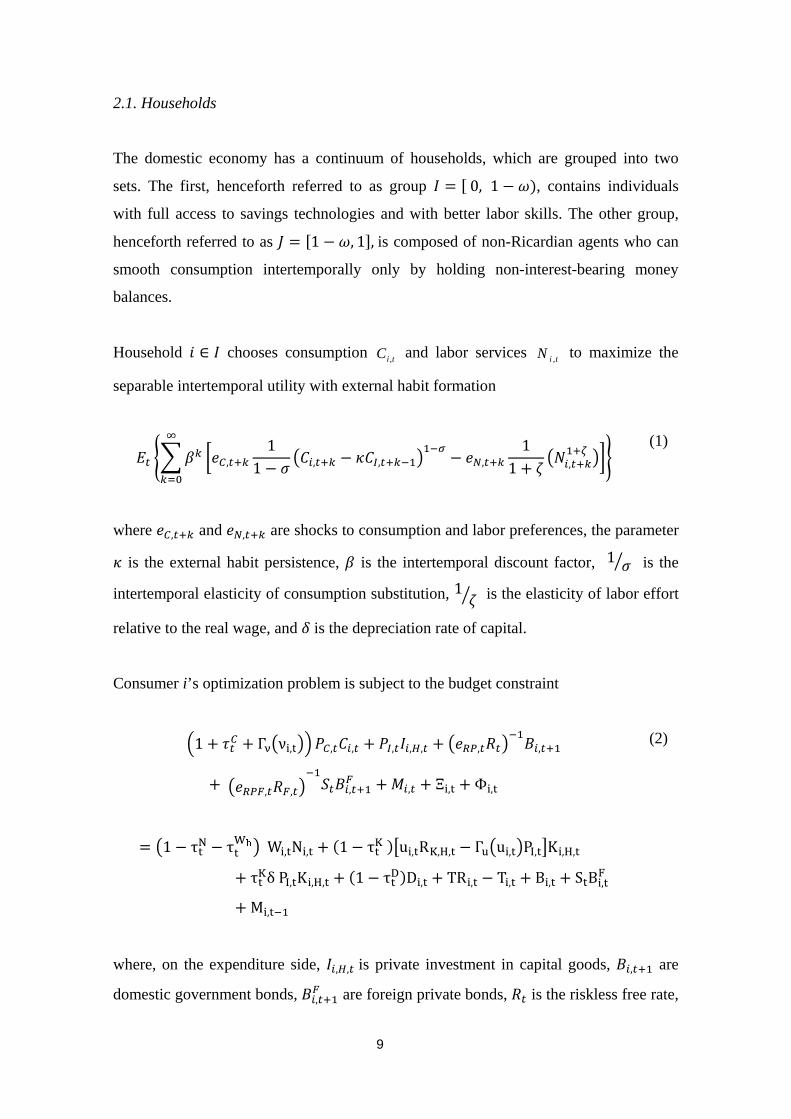
2.1. Households
The domestic economy has a continuum of households, which are grouped into two
sets. The first, henceforth referred to as group � � � 0, 1 ��, contains individuals
with full access to savings technologies and with better labor skills. The other group,
henceforth referred to as � �1 , 1�, is composed of non-Ricardian agents who can
smooth consumption intertemporally only by holding non-interest-bearing money
balances.
Household � � � chooses consumption tiC , and labor services tiN , to maximize the
separable intertemporal utility with external habit formation
�� �� �� ���,���
11 � ���,��� ���,����� ��,���
11 � � ���,���
� ���
���
(1)
where ��,��� and ��,��� are shocks to consumption and labor preferences, the parameter
� is the external habit persistence, � is the intertemporal discount factor, 1 �! is the
intertemporal elasticity of consumption substitution, 1 �! is the elasticity of labor effort
relative to the real wage, and " is the depreciation rate of capital.
Consumer i’s optimization problem is subject to the budget constraint
#1 � $�� � Γ��ν�,��' (�,���,� � (�,���,�,� � ����,�)��*�,��
� �����,�)�,��+�*�,��� � ,�,� � �,� � �,�
� �1 τ�� τ�
��� W�,�N�,� � 21 τ�� �3u�,�R�,�,� Γ��u�,��P�,�7K�,�,�
� τ��δ P�,�K�,�,� � 21 τ�
��D�,� � TR�,� T�,� � B�,� � S�B�,��
� M�,�
(2)
where, on the expenditure side, ��,�,� is private investment in capital goods, *�,�� are
domestic government bonds, *�,��� are foreign private bonds, )� is the riskless free rate,

10
)�,� is the interest rate on foreign bonds, ���,� and ����,� are risk premia over domestic
and international bonds, respectively, tS is the nominal exchange rate, ,�,� are money
holdings, Ξ�,� is a lump sum rebate on the foreign risk premium, and Φ�,� is the stock of
contingent securities negotiated within group I, acting as insurance against risks on
labor income. In addition, Γ��ν�,�� is a transaction cost on consumption and ν�,� is the
money-velocity of consumption. On the earnings side, W�,� is the wage earned by
household i for one unit of labor services, K�,�,� is the stock of private capital, u�,� is
teady state nominal e��u�,�� is the cost of deviating from the steady state rate of capital
utilization, R�,�,� is the gross rate of the return on private capital, D�,� are dividends, and
TR�,� are transfers from the government. Taxes are: $�� (consumption), $�
� (labor
income), $� ! (social security), $�
" (capital income), $�# (dividends) and ?�,� (lump sum,
active only for the foreign economy). Price indices are (�,� and (�,�, the prices of final
consumption and investment goods, respectively. Cost functions are detailed in the
Appendix.
The risk premium on internationally traded bonds follows:
����,� � ���� . exp DE���,�*�,�/G� H�� E���,% I�� I+��+�
J ∆+J � L���,�M
where ∆+ is the steady state change in the nominal exchange rate, H� is the steady state
foreign-debt-to-GDP ratio, and L���,� is a white noise shock. We let ���� correspond to
a steady state risk premium that allows for country-specific real interest rates. To this
end, we need to introduce the lump-sum rebate on the risk premium, Ξ�,�, so that these
flows do not impact the balance of payments of the foreign country5.
The accumulation of private capital follows the equation:
N�,�,�� � 21 "�N�,�,� � ��,� #1 ��I�,�,�/I�,�,��' ��,�,� (3)
5 For simplicity, we assume that Ξ�,� � Ξ�,�.

11
where ��,�,� is private investment, � is a cost to adjusting investment plans, and ��,� is a
shock to investment efficiency.
Households in group J are non-Ricardian agents that maximize a utility function
analogous to (1), but are refrained from carrying out investment decisions, except for
holding non-interest bearing money balances.
Within each group, households compete in a monopolistically competitive labor market.
By setting wage tiW , , household i commits to meeting any labor demand ., tiN Wages are
set à la Calvo, with a probability )1( Iξ− of optimizing each period. Optimizing
households in group I choose the same wage tiW ,
~, which we denote by tIW ,
~. Households
that do not optimize readjust their wages based on a geometric average of past and
steady state consumer inflation 1,1
2,
1,, : −
−
−
−
⎟⎟
⎠
⎞
⎜⎜
⎝
⎛= tiC
tC
tCti W
P
PW I
I
χ
χ
π . As the non-optimizing
wage does not perfectly track the trend growth of the economy, there will be wage
dispersion amongst households in the steady state6.
Household i’s optimization with respect to the wage tiW ,
~ yields the first order condition,
which is the same for every optimizing household in group I:
( ) ( )
( )0
~1
0
,,,
)1(
1,
1,
,
,,
, =
⎪⎪
⎭
⎪⎪
⎬
⎫
⎪⎪
⎩
⎪⎪
⎨
⎧
⎥⎥⎥⎥
⎦
⎤
⎢⎢⎢⎢
⎣
⎡
⎟⎟⎟⎟
⎠
⎞
⎜⎜⎜⎜
⎝
⎛
−
⎟⎟
⎠
⎞
⎜⎜
⎝
⎛−−Λ
∑∞
=
+++
−
−
−+
++++
+k
ktiktNktW
kC
tC
ktC
ktC
tIWkt
Nktkti
ktik
It
Nee
P
P
P
W
NEI
I
h
ζ
χ
χ
πττβξ
(4)
6 Brazilian employers do not have a tradition of automatically readjusting wages based on output growth. For this reason, we did not include output growth as a component in the automatic wage readjustment rule. However, it is possible that the business cycle somehow affects the likelihood that firms allow for wage readjustments in the first place. We leave this discussion for future work.

12
where tC
ti
P ,
,Λis the Lagrange multiplier for the budget constraint, and ktWe +, is, in the
absence of staggering, a time varying markup of the real wage: ��,� � ����,��� �
�1 � �� ��
����� � ��,� .
Equation (4) can be expressed in the following recursive form:
tI
tItNtW
tC
tI
G
Fee
P
WI
,
,,,
.1
,
, .~
.)1( =⎟⎟
⎠
⎞
⎜⎜
⎝
⎛−
+ ζη
ζω
where
⎪⎭
⎪⎬
⎫
⎪⎩
⎪⎨
⎧
⎟⎟
⎠
⎞
⎜⎜
⎝
⎛+
⎟⎟
⎠
⎞
⎜⎜
⎝
⎛
⎟⎟
⎠
⎞
⎜⎜
⎝
⎛= +
+
−+
+
1,
)1(
1,
1,
1
,
,, .
...: tI
CtC
tCtI
It
tC
tItI FEN
P
WF
I
II
I ζη
χχ
ζη
πππ
βξ
( )⎪⎭
⎪⎬
⎫
⎪⎩
⎪⎨
⎧
⎟⎟
⎠
⎞
⎜⎜
⎝
⎛+⎟
⎟
⎠
⎞
⎜⎜
⎝
⎛−−Λ= +
−
−+
1,
1
1,
1,
,
,,, .
....1: tI
CtC
tCtI
It
tC
tIWt
NttItI GEN
P
WG
I
II
I
h
η
χχ
η
πππ
βξττ
(5)
and ItN is households group I aggregate labor demanded by firms, and tIW , is
household group I’s aggregate wage index. Superscripts in the labor variable represent
demand. Subscripts represent supply.
Wage setting in group J is analogous to that of group I. The Calvo probability of
readjusting wages is )1( Jξ− and all other group-specific variables are expressed with
the j or J indices (respectively for individuals or for the group).

13
2.2 Production
The productive sector of the economy comprises firms that produce tradable
intermediate goods and non-tradable final goods. Price frictions are introduced only in
the block of intermediate goods firms.
2.2.1 Intermediate goods firms
Continuums of firms, indexed by [ ]1,0∈f , employ capital and labor services to produce
tradable intermediate goods tfY , under monopolistic competition. We introduce two
alternative ways in which public capital affects private productivity.
In the first specification, public capital augments factor productivity with no counterpart
in input costs. We label it “infrastructure approach to public capital”. Under this
approach, firm f’s production function is
( ) ( ) ( ) ( ) G
GG G
ttD
tftSH
tfGtttf KznNznKKzY α
αααα ψ −− −= 1
1
,,
,, ..... (6)
where DtfN , are aggregate labor services, G
tK is the stock of public capital, SHtfK ,
, are
private capital services, ψ are fixed costs that ensure zero profit in the steady state, and
tz and tzn are respectively (temporary) neutral and (permanent) labor-augmenting
productivity shocks. In equilibrium, HtftI
SHtf KuK ,,,
, = where HfK
is the stock of private
capital used by firm f.
In the second specification of the production function of intermediate goods, which we
label “mixed-capital economy”, we follow Valli and Carvalho (2010) and assume that
firms competitively rent capital services from the government, StfGK ,, , and from
households in group I, StfHK ,, , and transform them into the total capital input S
tfK ,
through the following CES technology:

14
( ) ( ) ( ) ( ) 11
,,1
1
,,1
, ..1−−
−−
−⎥⎦
⎤⎢⎣
⎡+−=
g
g
g
g
gg
g
g StfGg
StfHg
Stf KKK
ηη
ηη
ηηη
η ωω
(7)
where gω is the economy’s degree of dependence on government investment and gη
stands for the elasticity of substitution between private and public capital services, and
also relates to the sensitivity of demand to the cost variation in each type of capital.
The production function in the mixed-capital economy becomes:
( ) ( ) tD
tftS
tfttf znNznKzY ....1
,,, ψαα −= − (8)
where, in equilibrium, tftIS
tf KuK ,,, = , where tfK , is the stock of capital used by firm f.
For a given total demand for capital services, the mixed capital firm minimizes the total
cost of private and public capital services, solving:
StfG
GtK
StfH
HtK
KK
KRKRS
tfGS
tfH
,,,,,,,
min,,,,
+ (9)
subject to (7).
The rental rate for private capital services results from the equilibrium conditions in the
private capital market. The rental rate for government capital services also results from
equilibrium conditions, this time in the market for government capital services, but, in
steady state, we calibrate �� in order to let the rental rate for public capital goods
exclusively cover expenses with capital depreciation, so as to reproduce the fact that
public capital is usually subsidized7.
7 This assumption is also used in Macdonald (2008).

15
First order conditions to the problem of the mixed-capital firm yield the average rate of
return on capital and the aggregate demand functions for each type of capital
goods services:
( ) ( )( ) ggg G
tKgH
tKgtK RRR ηηη ωω −−− +−= 1
11
,
1
,, .).1(
(10)
St
tK
tGg
StG K
R
RK
gη
ω−
⎟⎟
⎠
⎞
⎜⎜
⎝
⎛=
,
,,
(11)
( ) St
tK
tHg
StH K
R
RK
gη
ω−
⎟⎟
⎠
⎞
⎜⎜
⎝
⎛−=
,
,, 1
(12)
All firms are identical since they solve the same optimization problem. The aggregate
composition of capital services rented by intermediate goods firms can be restated by
suppressing the subscript “f” from (7), using (10), and aggregating the different types of
capital services across firms:
( ) ( ) 11
,/1
1
,/1)1(
−−−
⎟⎟⎠
⎞⎜⎜⎝
⎛+−=
g
g
g
g
gg
gg S
tGgS
tHgSt KKK
ηη
ηη
ηηη
η ωω
(13)
Regardless of the approach to modeling public capital, we assume that firms rent labor
services from groups with unequal labor skills. We assume that the individuals that are
more constrained on their investment possibilities are also the ones with lower levels of
labor skills. This modeling strategy allows for a steady state where skillful workers can
earn more yet working the same amount of hours as the less skilled. In Brazil, labor
contracts usually stipulate an 8-hour work-day. The freely negotiable terms in labor
contracts are usually monthly nominal wages. The country is also globally known for its
uneven income distribution. The same can be said for the distribution of labor income.
According to the PNAD survey conducted by the Statistics Bureau (IBGE) in the year
2007, individuals earning less than 2 minimum wages (equivalent to USD 195 per

16
month at that time) amounted to 59.26% of the total economically active population.
The other share of the population earned almost 3 times as much in average.
The labor input used by firm f in the production of intermediate goods is a composite of
labor demanded to both groups of households. In addition to a population-size
adjustment (ω ) to the firm’s labor demand, we add the parameter [ ]ωω1,0∈v to
introduce a bias in favor of more skilled workers. The resulting labor composite obtains
from the following transformation technology
( ) ( ) ( )( ) )1/(/11
,/1/11
,/1
, )1(:−−− +−=
ηηηηω
ηηω ωω J
tfI
tfD
tf NvNvN (14)
where
( ))1/(
1
0
/11
,
/1
, 1
1:
−−−
⎥⎥⎦
⎤
⎢⎢⎣
⎡⎟⎠
⎞⎜⎝
⎛
−= ∫
II
I
I
diNN itf
Itf
ηηωη
η
ω
(15)
( ))1/(
1
1
/11
,
/1
,
1:
−
−
−
⎥⎥⎦
⎤
⎢⎢⎣
⎡⎟⎠
⎞⎜⎝
⎛= ∫JJ
J
J
djNN jtf
Jtf
ηη
ω
ηη
ω
(16)
and where η is the price-elasticity to demand for specific labor bundles, Iη and Jη are
the price-elasticities for specific labor varieties. The special case when 1=ωv
corresponds to the equally skilled workers.
Taking average wages ( tIW , and tJW , ) in both groups as given, firms choose how much
labor to hire by minimizing total labor cost JtftJ
ItftI NWNW ,,,, + subject to (14). It
follows from first order conditions that the aggregate wage is
[ ] ηηω
ηω ωνων −−− +−= 1
11,
1, ..)..1( tJtIt WWW
(17)

17
and the aggregate demand functions for each group of households are:
Dt
t
tIIt N
W
WN .)..1( ,
η
ω ων−
⎟⎟⎠
⎞⎜⎜⎝
⎛−=
(18)
Dt
t
tJJt N
W
WN ... ,
η
ω ων−
⎟⎟⎠
⎞⎜⎜⎝
⎛=
(19)
Intermediate goods prices are set under monopolistic competition, with Calvo-type price
rigidities. We assume local currency pricing. Let tfHP ,, and tfXP ,, be the prices for
goods sold by firm f in the domestic and foreign markets, with Hξ and Xξ denoting the
probability that the firm will not optimize prices in each of these markets. Non-
optimizing domestic and foreign firms adjust their prices according to the rules
( ) 1,,1
2,
1,,, : −
−
−
−
⎟⎟
⎠
⎞
⎜⎜
⎝
⎛= tfHH
tH
tHtfH P
P
PP H
H
χχ
π
(20)
( ) 1,,1
2,
1,,, : −
−
−
−
⎟⎟
⎠
⎞
⎜⎜
⎝
⎛= tfXX
tX
tXtfX P
P
PP X
X
χχ
π
(21)
where Hπ and Xπ are domestic and foreign intermediate goods’ steady state inflation
rates.
Optimizing firms choose the prices tfHP ,,
~ and tfXP ,,
~ to maximize the expected
discounted sum of nominal profits:
( )⎥⎦
⎤⎢⎣
⎡ +Λ∑∞
=+++
0,,,,,, )()(
kktfX
kXktfH
kHkttIt DDE ξξ
(22)
where kttI +Λ ,, is household I’s average discount factor, given by

18
diP
P
ktC
tC
ti
ktikkttI
+
−+
+ ∫ ΛΛ
−=Λ
,
,1
0 ,
,,, 1
1 ω
βω
(23)
and nominal profits, net of fixed costs, are defined as
( ) tfttfHtfH HMCPD ,,,,, −= (24)
( ) tfttfXttfX XMCPSD ,,,,, −=
(25)
Optimization is subject to the price indexation rule, to domestic and foreign demand for
firm f’s goods, tfH , and tfX , , taking as given the marginal cost, the exchange rate and
aggregate demand.
First order conditions for the pricing decisions yield
( ) 0~
)(0
,,)1(
1,
1,,,, =
⎥⎥
⎦
⎤
⎢⎢
⎣
⎡
⎟⎟
⎠
⎞
⎜⎜
⎝
⎛−⎟
⎟
⎠
⎞
⎜⎜
⎝
⎛Λ∑
∞
=+++
−
−
−++
kktfktktP
kH
tH
ktHtHkttI
kHt HMCe
P
PPE H
H
χχ
πξ
(26)
and
( ) 0~
)(0
,,)1(
1,
1,,,, =
⎥⎥
⎦
⎤
⎢⎢
⎣
⎡
⎟⎟
⎠
⎞
⎜⎜
⎝
⎛−
⎟⎟
⎠
⎞
⎜⎜
⎝
⎛Λ∑
∞
=+++
−
−
−+++
kktfktktP
kX
tX
ktXtXktkttI
kXt XMCe
P
PPSE X
X
χχ
πξ (27)
where tPe , represents a time-varying markup of prices in the absence of staggering, with
��,� � ����,��� � �1 � �� �
���� � ��,� , where ��,� is white noise. For simplicity we
assume that the markup processes for both domestic and exported goods are the same.
As firms are identical, they face the same optimization problem, choosing the same
optimal price tHtfH PP ,,,
~~ = and tXtfX PP ,,,
~~ = .

19
Pricing equations (26) and (27) can be restated recursively as
��,�
�,�
� ��,��,�
�,�
(28)
��,��,�
� ��,��,��,�
(29)
where
⎪⎭
⎪⎬
⎫
⎪⎩
⎪⎨
⎧
⎟⎟
⎠
⎞
⎜⎜
⎝
⎛+= +−
+
+
+Λ1,1
,
1,
1,
1,, .
..... tX
XtX
tX
tC
t
tXtttX FEXMCFXX
I
θ
χχ πππ
ππ
βξ
⎪⎭
⎪⎬
⎫
⎪⎩
⎪⎨
⎧
⎟⎟
⎠
⎞
⎜⎜
⎝
⎛+= +
−
−+
+
+Λ1,
1
1,
1,
1,
1,,, .
...... tX
XtX
tX
tC
t
tXttXttX GEXPSGXX
I
θ
χχ πππ
ππ
βξ
Aggregating over firms, domestic and export intermediate goods prices are
( )[ ] )1/(11
,1
,, .)~
).(1( θθθ ξξ −−− +−= tHHtHHtH PPP
(30)
⎪⎭
⎪⎬
⎫
⎪⎩
⎪⎨
⎧
⎟⎟
⎠
⎞
⎜⎜
⎝
⎛
ΛΛ+= +−
++1,1
,
1,
,*
1,*
, ..: tHHtH
tH
tI
tI
tHtttH FEHMCFHH
θ
χχ πππ
βξ
⎪⎭
⎪⎬
⎫
⎪⎩
⎪⎨
⎧
⎟⎟
⎠
⎞
⎜⎜
⎝
⎛
ΛΛ+= +
−
−++
1,
1
1,
1,
,*
1,*
,, ..: tHHtH
tH
tI
tI
tHttHtH GEHPGHH
θ
χχ πππ
βξ

20
( )[ ] )1/(11
,1
,, .)~
).(1( θθθ ξξ −−− +−= tXXtXXtX PPP
(31)
2.2.2 Final goods firms
The economy has three firms producing non-tradable final goods. One specializes in the
production of private consumption goods, another in public consumption goods, and the
third in investment goods. Except for the firm that produces public consumption goods,
all final goods’ producers combine domestic and imported intermediate goods in their
production line.
To produce private consumption goods, CtQ , the firm purchases bundles of domestic
CtH and foreign C
tIM intermediate goods. To adjust its imported share of inputs, the
firm faces the cost ⎟⎟⎠
⎞⎜⎜⎝
⎛Γ tIMC
t
Ct
IMe
Q
IMC ,, , where ���,� is an import demand shock.
Letting Cν denote the bias towards domestic intermediate goods, the technology to
produce private consumption goods is
[ ]( )[ ]
)1/(
/11/1
/11/1
)/(1)1(
)(:
−
−
−
⎪⎭
⎪⎬⎫
⎪⎩
⎪⎨⎧
Γ−−
+=
CC
C
CC
CC
Ct
Ct
CtIMC
CtCC
tIMQIM
HQ
μμ
μμ
μμ
ν
ν
(32)
where
)1/(
/11, )(:
−
−
⎟⎟
⎠
⎞
⎜⎜
⎝
⎛= ∫
θθ
θ dfHH Ctf
Ct
)1/(
*/111
0,
**
*
* )(:
−
−⎟⎟⎠
⎞⎜⎜⎝
⎛= ∫
θθθ dfIMIM C
tf
Ct

21
The firm will minimize total input costs
CttIM
CttH
IMH
IMPHPCt
Ct
.. ,,,
min +
(33)
subject to the technology constraint (32) taking intermediate goods prices as given.
The existence of an adjustment cost to the share of imported goods in the production of
final goods invalidates the standard result that the Lagrange multiplier of the technology
constraint equals the price index of final goods. The price index of private consumption
goods that ensures that the producing firm operates under perfect competition is8:
( ) ( ) CC Ct
CttCP
μμ λ−Ω= 1
,
(35)
where
( )( )[ ] CC
CC Ct
CtIMtIMCtHC
Ct QIMPP μμμ ννλ −−ℑ− Γ−+= 1
11
,1
, )/(/1
(35)
( ) ( )( )
C
CC
C
CC
Ct
CtIMtIM
Ct
CtIM
Ct
CtIM
CtHCCt
QIMP
QIM
QIMP
μ
μ
μ νν−
−ℑ
ℑ−
⎪⎪⎭
⎪⎪⎬
⎫
⎪⎪⎩
⎪⎪⎨
⎧
Γ×
⎟⎟
⎠
⎞
⎜⎜
⎝
⎛
Γ−Γ
−+=Ω 1
1
1
,
1,
)/(/
)/(1
)/()1(
(36)
In general, first order conditions and equation (34) can be combined to yield the
following demand equations:
Ct
tC
tH
Ct
tHC
Ct Q
P
PPH
CCμμ
ν−−
⎟⎟
⎠
⎞
⎜⎜
⎝
⎛⎟⎟⎠
⎞⎜⎜⎝
⎛
Ω=
,
,
1
,
(37)
8 Details of the derivation of (34) are shown in Valli and Carvalho (2010).

22
)/(1
)/(/)1(
,
,
1
,
Ct
CtIM
Ct
tC
Ct
CtIMtIM
Ct
tCC
Ct QIM
Q
P
QIMPPIM
C
CC
C
Γ−⎟⎟
⎠
⎞
⎜⎜
⎝
⎛ Γ⎟⎟⎠
⎞⎜⎜⎝
⎛
Ω−=
−ℑ− μμ
ν
(38)
The description of the model for investment goods is analogous, and the import demand
shock that affects the cost to adjust the import basket is exactly the same.
2.3 Fiscal authority
The domestic fiscal authority pursues a primary surplus target ���� expressed in terms
of GDP, levies taxes on consumption, labor, capital and dividends, makes biased
transfers, and adjusts expenditures and budget financing accordingly.
To account for the fact that the focal fiscal variable in Brazil is the (net-of-interest)
primary balance, we introduce a rule for the primary surplus that responds to business
cycle conditions and to the deviations of the public debt-to-GDP ratio from its
steady-state:
( ){ } ( ) tspYtYgyspYtYBsp
tspt
ggbbsp
spsp
Y ,1,,,
1
).1(
.
εφφρρ
−−+−+−
+=
−
−
(39)
where sp is the primary surplus target,ttY
tt YP
SPsp
.,
= , tSP is the nominal level of the
primary surplus, 11,
,−−
=ttY
ttY YP
Bb ,
1,
−
=t
ttY Y
Yg , the unindexed counterparts are steady-
state ratios, and tsp,ε is a white noise shock to the primary surplus.
We introduce social programs in the form of biased transfers of public funds. Total
transfers ( tTR ) are distributed to each household group according to:

23
ttr
tI TRv
TRω
ω−
−=
1
).1(:,
(40)
ttrtJ TRvTR .:, =
(41)
where trv is the bias in transfers in favor of group J, and
ttrttY
ttrtr
ttY
t
YP
TRtr
YP
TR,
,, ..).1(
.ερρ +⎟
⎟
⎠
⎞
⎜⎜
⎝
⎛+−=⎟
⎟
⎠
⎞
⎜⎜
⎝
⎛ (42)
where tr is the steady state value of government transfers, and ttr ,ε represents a white
noise shock.
Government’s capital accumulation follows the equation
��,��� � �1 � ����,� �,� �1 � � I,/I,���� ��,�
where ��,� is public investment and, for simplicity, �,� is the same shock to the
efficiency of investment that affects private capital accumulation.
Government investment follows an autoregressive rule of the form
( ) tigtigigt igigig ,1..1 ερρ ++−= − (43)
The government budget constraint is thus
( )( )
0.
....
.).)((..).(
,,1
,,,,1
1
,
,,,,,
=−−−−−+++++
+Γ−++++
−
+−
tGtIt
ttttGtGtGtIttttRPttDt
ttItIutItKKt
Dtt
Wt
Wt
NtttC
Ct
IPM
BTRGPKRuMBReTD
KPuuRNWCP fh
τ
δτττττ
(44)

24
with �� � 0 for the domestic economy. Equation (44) can be recast in terms of the
primary surplus:
( ) )().( 11
1
−+− −−−= ttttRPtt MMBReBSP (45)
The former expression makes it clear that, in this model, money not only has an
effective role in real decisions, but also matters for the adjustment of fiscal accounts.
Increased money supply can alleviate the financial burden from public debt, a feature
that approximates the theoretical model to the real conduct of economic policy.
As the primary surplus can also be stated as the difference between public revenues and
expenditures, government consumption in this model will adapt endogenously so that
the other fiscal instruments follow their stated rules.
2.4 Monetary authority
The monetary authority sets nominal interest rates and issues as much money as
demanded by the public. To set interest rates, it follows a forward-looking rule that is
compatible with an inflation targeting regime
( ) tRt
teYtYg
tC
tCtRtRt
SS
Sgg
P
PERRR
Y ,4
4
11,
1,
3,441
4 ).1(.
εφφ
φφφ
+⎥⎥
⎦
⎤
⎢⎢
⎣
⎡Δ−⎟⎟
⎠
⎞⎜⎜⎝
⎛+−+
⎥⎥⎦
⎤
⎢⎢⎣
⎡
⎟⎟
⎠
⎞
⎜⎜
⎝
⎛Π−+−+=
−−
−
+Π−
(46)
where Π is the annual inflation target, 4R is the annualized quarterly nominal
equilibrium interest rate, which satisfies Π= − .44 βR , Yg is the steady state output
growth rate, SΔ is the steady state nominal exchange rate variation, and tR ,ε is a white
noise shock to the interest rate rule.

25
3 Bayesian Estimation
We estimate the parameters for the domestic economy using Bayesian inference
methods9. Below are the procedures adopted to this end.
3.1 Calibration
First we stationarize the model so that the variables are expressed as shares of GDP.
Except for hours worked, real variables are divided by real GDP to handle the unit root
that arises from the permanent labor productivity shock and, in the case of the
infrastructure approach to public capital, from the trend in public capital. Nominal
variables are transformed to shares of nominal GDP as prices also trend due to our
assumption of non-null steady state inflation.
The foreign economy is entirely calibrated, following the parameterization presented
in CMS.
Some parameters of the domestic economy are calibrated. Following the standard
procedure, price levels and capital utilization are normalized to 1, while profits and
adjustment costs are set to zero. Some endogenous variables are calibrated so as to
reproduce Brazilian historical averages during the inflation targeting regime (Table 1),
and they consequently pin down the steady state values for most of the remaining
endogenous variables of the model.
Most of the parameters that affect the steady state of the model were also calibrated.
Their values are shown in Table 2. In the absence of reasonable proxies in the literature
for Brazil, some of these parameters were set at the same values as in CMS. A few
others were calibrated to ensure that some desired relations hold in the steady state. The
labor demand bias, ων , for instance, was calibrated to ensure that households’ groups I
9 We use Dynare to conduct the log-linear approximation of the model to the calibrated steady state and to perform all estimation routines. We run 2 chains of 2 million draws of the Metropolis Hastings to estimate the posterior.

26
and J work the same amount of hours. The home biases Cν and Iν were obtained from
the demand equations of imported goods using the steady state value of consumption
and investment goods, in addition to the quantum of imports.
With the exception of consumption taxes, Cτ , which were calibrated following Siqueira
et. al. (2001), Brazilian tax rates were set based on the current tax laws.
Notwithstanding, these laws allow for a great variety of exemptions and usually
differentiate tax rates according to taxable bases. As such, they are not concise
references for calibration. However, to our knowledge there is no aggregate data we
could refer to for such a purpose, and so we chose the tax rates that are most
commonly applied.
We calibrated the price-elasticity to demand of government investment goods, gη , to a
value that is close to 1, arbitrarily approximating it to a Cobb-Douglas technology. This
enabled us to calibrate gυ from the rental rate for government capital, which we
assumed to be just enough to cover expenditures with depreciation.
In lack of quarterly data on household distribution, the wage indexation parameter of
non-Ricardian households was set so as to equal the estimated mean of the same
parameter for Ricardian households. The Calvo-probabilities of price optimization in
the intermediate goods sector, �� and ��, were also fixed, as attempts to estimate them
resulted in a wide region of model indeterminacy. They were set at 0.30, a value that
closely reflects the average price rigidity in Brazilian CPI-micro-data, which is of about
1.3 quarters (Gouvea, 2007).
3.2 The data
We used the following (seasonally-adjusted) time series to estimate the parameters of
the domestic economy:
27
• Consumer inflation ��,�: quarterly inflation of the IPCA (Índice de Preços ao
Consumidor Amplo – IBGE);
• Nominal interest rate ��: quarterly effective nominal base rate (Selic);
• Total investment ��,��� ��,��� : seasonally adjusted quarterly nominal flows of
gross fixed capital formation and inventory change in the national accounts as a
share of quarterly GDP;
• Exports ��,�� ��,��� : seasonally adjusted quarterly nominal flows of exports in
the national accounts as a share of quarterly GDP;
• Exports inflation ��,�: quarterly inflation rate of Brazilian export prices
calculated in USD by Funcex;
• Exports ��,���� ��,��� : seasonally adjusted quarterly nominal flows of imports
in the national accounts as a share of quarterly GDP;
• Private consumption ��,��� ��,��� : seasonally adjusted quarterly nominal flows
of household consumption in the national accounts as a share of quarterly GDP;
• Government consumption �,� � ��,��� : seasonally adjusted quarterly nominal
flows of government expenditures in the national accounts as a share of
quarterly GDP;
• Installed capacity utilization ��,�: quarterly capacity utilization published by
FGV, normalized using the average of the series;

28
• Exchange rate variation �� ��� � : quarterly nominal BRL/USD exchange rate
variation;
• Primary surplus ���: seasonally adjusted primary surplus of the consolidated
government (methodology that does not include Petrobrás in the public sector10)
as a share of GDP.
The data were sampled from the inflation targeting period in Brazil (1999:Q1 to
2010:Q2). From 1994 to 1998, although inflation was low, monetary policy followed a
fixed exchange rate band regime. To avoid contamination of estimations with such an
important structural break, we chose to use the smaller sample.
As Guerron-Quintana (2007) pointed out, the data set chosen for the estimation matters
for parameter identification. In our attempt to include the most number of series
available, we noticed that the inclusion of monetary aggregates and available labor
market series destabilized the estimations, and maximization algorithms could generally
not find any optimum. We thus chose to exclude them from our data sample.
3.3 Shocks
We estimate the model with the following shocks:
• Total factor productivity, �
• Labor productivity, ��
• Consumption preferences, ��
• Monetary policy, ��
• Primary surplus, ���
• Public transfers, ���
10 As the series for the primary surplus excluding Petrobrás is only available from 2002:Q1 on, we regressed the series with and without Petrobrás using the sample when both are available to obtain an estimate of the primary surplus without Petrobrás for the period 1991:Q1 to 2001:Q4.

29
• Gap between domestic and foreign
labor productivity, ����
• Foreign risk premium, ����
• Domestic risk premium, ���
• Import bias, ��
• Government investment, ���
• Investment efficiency, ��
• Wage markup, ��
• Price markup, ��
The shock to labor preferences, ��, was too poorly identified in the initial rounds of
estimation and was dropped from the final estimation reported in this paper.
Except for monetary policy and primary surplus shocks, which are white noise, all other
shocks follow AR processes that converge to a steady state. In the mixed-capital
economy, we assume that the process that governs the labor productivity shock follows:
tznt
tznzn
t
t
zn
zngy
zn
zn,
2
1
1
.).1( ερρ ++−=−
−
−
(47)
where gy is the steady state output growth, which also equals the steady state rate of
labor productivity under this approach to public capital. In addition, tzn ,ε is an
exogenous white noise process. We also assume that the normalized labor-augmenting
technology shock in the domestic economy can temporarily deviate from that of the
foreign economy:
trzntrznrznrznrznt
ttrzn ee
zn
zne ,1,
*
, .).1( ερρ ++−=≡ −
(48)
where *
**
t
tt Y
znzn = and
t
tt Y
znzn = and trzn ,ε is a white noise shock.
30
For the infrastructure approach to public capital, there are two sources of trending
growth in the economy, and so the process that governs the labor productivity shock is:
tznt
tznzn
t
t
zn
zngy
zn
zn G
,2
111
1
.).1( ερρ αα
++−=−
−−−
−
(47’)
and the difference in the normalized shock to domestic labor productivity from that in
the foreign economy follows:
trzntrznrznrznrznt
ttrzn ee
zn
zne ,1,
*
, .).1( ερρ ++−=≡ −
(48’)
where, in this case, *
*
11
*
**
αα−
−=
G
t
tt
Y
znzn and
αα−
−=
11 G
t
tt
Y
znzn .
The steady state of the shocks to the wage and price markups are respectively �
��� and
�
��� . Measurement errors were also included for national accounts series, as, in addition
to suffering from substantial and frequent revisions, these series do not incorporate
federal companies’ financial flows into government accounts.
3.4 Estimation
The parameters were estimated after the model was log-linearized around the steady
state. Table 3 shows prior and posterior moments.
For the choice of prior means, we used information from Brazilian-specific empirical
evidence, whenever available, or took an agnostic stance of setting the priors at the
center of traditionally chosen distributions or at the mode of the posteriors reported for
the Euro Zone in CCW. In general, our priors were more diffuse than those in CCW.
Below is a more detailed description of the priors we set based on Brazilian data:

31
• The priors for the coefficients in the primary surplus rule were set at the point
estimates of the partial-equilibrium regression shown in Valli and Carvalho
(2010), run on a sample from 1996 to 2009.
• For the monetary policy rule, our prior means were set at the point estimates of
the Taylor rule presented in Minella and Souza-Sobrinho (2009)11.
• The prior means for the autoregressive components of the shocks were
agnostically set at 0.5, corresponding to the center of beta or uniform
distributions in the [0,1] interval. The only exception was the shock to the wage
markup, with a mean set at the NAWM mode.
The estimated data density favored the model where public capital is taken as an
externality to firms (the infrastructure approach). For the same choice of priors we have
just described, excluding the exchange rate component in the Taylor rule, the Lapplace
approximation to the log data density of the mixed capital model was 977.77, compared
to 1003.65 obtained under the infrastructure approach. In the analysis that follows, we
report the estimates of the model under the infrastructure approach to public capital,
assuming that there is an exchange rate component in the Taylor rule.
Figure 4 shows plots of the prior and posterior distributions for each estimated
parameter, and Figure 5 shows convergence diagnostics. Some of the shapes of the
posteriors are not well behaved (sometimes non-smooth or multimodal) in spite of a
reasonable number of draws in each chain of the Metropolis Hastings algorithm12. The
analyses that follow are based on the posterior means as calculated in the standard code
of Dynare.
11 Our policy rules were estimated with only one lag in the policy instrument. The prior mean for the autoregressive components were thus set as the sum of the point estimates of the two lags in the individual regressions we just mentioned. 12 So far, the computational resources available to this project have not allowed us to successfully handle estimates with a much greater number of draws.

32
The estimated means suggest that price and wage indexation in Brazil is substantially
higher than in the Euro Zone13. Notwithstanding, monetary policy in Brazil is much
more responsive to deviations of inflation from the targets. The response to output
conditions is practically null, a result that was also obtained in partial-equilibrium
regressions presented in Minella and Souza-Sobrinho (2009). Still compared to the Euro
Zone, the autoregressive component of the rule in our estimations is much higher, and
we also find a significant, yet small, response of the policy rate to exchange
rate variations.
The estimated primary surplus rule is less responsive to the public debt than suggested
by the partial equilibrium regression presented in Valli and Carvalho (2010). The fiscal
response to the business cycle is practically negligible. As such, the fiscal rule is very
close to a simple autoregressive rule, with a moderate autoregressive component (0.55).
Inertia in public investment is relatively high (0.786), contrasting with the low
regressiveness of public transfers (0.332).
4 Impulse Responses and Shock Decomposition
4.1 Impulse responses to fiscal Shocks
Figures 6 to 8 show impulse responses to shocks to fiscal variables in the model. The
median responses are shown in bold lines, within the 90% confidence interval plotted
with thinner lines, drawn from the posterior distribution. The shocks are in the
magnitude of a 1 standard deviation from the steady state of the variables they directly
affect.
An expansionist shock to the primary surplus (as a share of GDP) leads to increases in
both government consumption and public investment (both in levels and as shares of
GDP). This heats the economy as intermediate goods firms attempt to meet the
increased demand for their goods. Firms are able to hire more labor, under a marginal
13 We take CCW as a reference for Euro Zone estimates.

33
reduction in real wages. This triggers an expansion in private consumption, which,
together with the rise in government consumption, sustains output levels above the trend
for over a year. The increased demand for consumer goods allows for the pass-through
of the intermediate goods inflation to consumer prices, and thus consumer inflation
rises. Monetary policy reacts to the inflationary conditions expected for the future and
helps bring inflation back to the steady state. The interest rate reaction is not too intense
because of the forward lookingness of the rule. Most of the effects of the primary
surplus shock, including that on output, fade out within two years. The increase in the
ratio of public debt to GDP, however, is very long-lasting.
An expansionist shock to government transfers (as a share of GDP) also has short-lived
effects but the cycles it creates are quite different from those of the primary surplus
shock. The transfers shock requires a strong reduction in government consumption and
public investment (both as a share of GDP) so that the primary fiscal rule is fulfilled. As
the transfers are biased towards the population that has restricted access to investment,
consumption in this group rises above the trend. Yet, the increase in private
consumption is not enough to ensure output expansion upon impact of the shock. It is
only when government consumption returns to the steady state and thus stop depressing
the demand for intermediate goods that output can take advantage of the greater demand
from consumers and momentarily peaks above the trend. The shock to transfers has a
mild and short-lived inflationary impact, likely due to the fact that the autoregressive
component of the transfer rule is low, allowing the shock to dissipate fast.
An expansionist shock to government investment (as a share of GDP) requires a
significant reduction in the ratio of government consumption to GDP so that the primary
surplus rule is fulfilled. However, as the output strongly accelerates from the increased
demand for intermediate goods to produce investment goods, detrended levels of
government consumption fall only in the initial quarters, recovering soon after. The
boost in output helps reduce the debt-to-GDP ratio, and the primary fiscal rule can also
act so as to enact expansionary effects upon the economy. A heated labor market allows
for a substantial increase in private consumption, with an important inflationary impact.
The impact on CPI inflation is much stronger than that observed after a shock to the
34
primary surplus, but it fades out a little faster. The effects on real variables, including
those on output, are long-lasting.
4.2 Impulse responses to the other shocks
Figure 9 shows the impulse response to a monetary policy shock. As expected, the
shock drives output down, by depressing investment and private consumption. Firms cut
down on their demand for labor, and employment falls. The rise in interest rates puts
pressure on the debt service, which in turn requires a reduction in government
consumption that further dampens output. The nominal exchange rate appreciates. All
these effects result in a drop of intermediate goods inflation, passing through to
consumer prices. The trough in inflation is in the first quarter after the shock hits
the economy.
It is not clear what one should expect for the shape of the response of consumer
inflation to a monetary policy shock in Brazil. Figure 10 replicates the responses
obtained in Minella (2001), where he estimates a monthly VAR for the period 1994:09
to 2000:12 with standard endogenous variables in addition to the country risk premium.
All of the responses are hump-shaped, but the trough occurs within the first three
months after the shock. However, if we update the estimations to include the most
recent data, the responses show a price puzzle in the first three months, and the trough is
achieved later, in the sixth month (Panel A of Figure 11). If we use the same set of
endogenous variables to estimate a quarterly VAR imposing the same ordering as in
Minella (2001), we obtain greater uncertainty in the responses, with the central
prediction indicating troughs in the 2nd and 5th quarters (Panel B of Figure 11). The
shape of the response also considerably changes if we replace industrial production by
GDP in the set of regressors (Panel C of Figure 11). In this case, the evidence of a price
puzzle remerges and the trough of the response distinguishably occurs in the 5th quarter.
Finally, if we replace the country risk premium for the nominal exchange rate in the set
of regressors (Panel D of Figure 11), we find a completely different response where
inflation does not drop after a shock to the exchange rate.

35
Figure 12 shows the impulse responses of a shock to the domestic risk premium. The
shape of the responses resemble those of a monetary policy shock, as, similarly to the
shock to the interest rate, the shock to the domestic risk premium represents a higher
cost of borrowing to the government and a higher opportunity cost for investment. After
the shock, the monetary policy instrument is fine-tuned to try to counterbalance the
contractionist impact of the shock to the domestic risk premium.
Figure 13 shows the impulse responses of a shock to the foreign risk premium. It first
transmits through the UIP, and as the shock hits, the exchange rate depreciates.
Favorable terms of trade help boost exports and dampen imports, causing output to rise
up above the trend. Greater labor demand helps private consumption to increase.
Demand pressures feed through intermediate and consumer prices, and monetary policy
reacts to get inflation back on the steady state.
Figure 14 shows the impulse responses to a temporary total factor productivity shock.
On impact, the shock allows firms to cut down on their (nominal) marginal cost and on
labor demand. As the prices of intermediate goods are set as a markup over marginal
costs, they fall after the shock hits. Their passthrough to the GDP deflator implies a
slight increase in real wages. Both factors, price drops and real wage increases, are
factored into consumer decisions, and thus private consumption rises. Price drops of
intermediate goods are also translated into reductions in export prices, partially
compensated by a depreciated exchange rate. The rise in demand from consumers,
investors and exporters allows output to enact a substantial expansion, so high as to
allow government consumption to rise above the trend yet keeping its share to GDP
below the steady state for a number of quarters.
In contrast, a shock to permanent (labor-augmenting) productivity (Figure 15) implies a
rise in firms’ demand for labor, putting pressure on real wages. The rise in marginal
costs and the increased demand for final consumption and investment goods translate
into generalized price increases.

36
4.3 Historical decomposition
Figure 16 shows the historical decomposition of key macroeconomic variables in Brazil
during the inflation targeting regime. As the plots with all shocks to the model are
visually messy, we chose to depict only the shocks that mostly impacted each series.
Monetary policy shocks, which are traditionally interpreted as shocks to policymakers’
preferences, have played a minor role in the setting of nominal interest rates in Brazil.
Overall, shocks to firms’ productivity, domestic risk premium and price markups have
been more influential in the setting of the monetary policy rate.
Productivity shocks have also played a significant role in the cycles of consumer
inflation, primary surplus to GDP and consumption to GDP. As the model implies
close correspondence of (permanent) labor-productivity shocks in the domestic and
foreign economy, it is customary to interpret these shocks as a transmission channel of
global shocks to the domestic economy. The importance of such shocks in the
decomposition of historical series should thus be reflecting the fact that Brazil has been
often hit by a number of shocks stemming from abroad.
Aside from technological shocks, the domestic risk premium and price markup shocks
have also been highly influential to inflation in Brazil. The plots suggest that, more
recently, price markups have been the main upward-pressing force to consumer inflation
in the country.
As to the primary surplus to GDP, fiscal policy shocks have been quite important as
well. Until 2003, the shocks to fiscal preferences were usually in the direction of
enacting expansionist policies so as to countervail the contractionist impact of
productivity shocks. This reversed in 2004, and from then to a few months after the
global financial crisis of 2008, fiscal policy preferences were contractionist. The crisis
triggered the reversal of fiscal policy preferences towards expansionist decisions.
Moreover, domestic risk premium shocks have put substantial downward pressure to
primary surpluses.

37
As to private consumption (as a share of GDP), expansionist shocks were mainly
technology shocks and shocks to public transfers and public investment, especially after
2003, coinciding with the presidential term of Mr. Lula. The domestic risk premium
was the main shock pushing consumption downwards.
5 Policy exercises
Figures 17 to 21 show policy exercises carried out with simulations of the model at the
mean of the estimated posterior distribution of the parameters.
After the global financial crisis in 2008, the Brazilian government has systematically
attained lower than targeted primary surpluses. In 2010, amid presidential elections, the
future maintenance of the target levels was even called into question. Figure 17 shows
what would happen to the main dynamics of the economy should the target for the
primary surplus be drastically cut down to 1.5% of GDP. The dynamic responses of
output and inflation would not post relevant changes under the parameterized model.
However, for this new target to be sustainable, which is to say in other words that for
the model to have a well-defined equilibrium, the public debt to GDP ratio should be
cut off in more than half.
Figure 18 shows what one can expect for the model dynamics if the government
increases its commitment to the steady-state level of public debt as a share of GDP. If
the response to the debt in the fiscal rule increases almost tenfold, from the estimated
0.017 to 0.10, the same expansionist shock to the primary surplus rule causes output to
initially expand by the same amount, yet returning to the steady state a little more
sluggishly. Inflation rises a little more and is also a little more persistent to return to the
steady state. The most pronounced change is in the public debt path, which reverses
back to the steady state a lot faster. If the response to debt in the fiscal rule is increased
to 0.20, the dynamic responses of the model become highly cyclical, reaching regions of
indeterminacy for values of the debt coefficient in the fiscal rule higher than 0.20.

38
Figure 19 shows an analogous exercise, where instead we change the response of the
fiscal rule to output growth. Increasing the reaction of the primary surplus to output
growth from 0.038 to 0.10 causes relatively little changes in the dynamics of output,
inflation, debt and the primary surplus. However, if the reaction hikes to 0.50, the
dynamic responses of the model to a primary surplus shock become extremely cyclical.
On the other hand, if the monetary authority chooses to react more to output growth
(Figure 20), contractionist shocks to the interest rate generally produce muter
dynamic responses.
We also conduct exercises changing the share of non-Ricardian agents in the population
(Figure 21). We find an important sensitivity of the dynamics of real variables to this
feature of the model. The lower the share of non-Ricardian agents, the muter the
responses of real variables to a fiscal shock to the primary surplus. This result is in line
with the literature. In Galí et. al. (2004), the sensitivity of aggregate consumption
responses to a government spending shock is attributed to the presence of rule-of-thumb
consumers, calibrated at 50%, and to the presence of sticky prices. Notice, however, that
in our model non-Ricardians make intertemporallly optimal decisions, yet under
restrained investment options.

39
6 Conclusion
In this paper, we employ Bayesian methods to estimate the parameters of the Brazilian
economy, modeled as an open-economy where fiscal policy is implemented through a
rich set of instruments: primary surplus, public investment, and social transfers. There
are both Ricardian and non-Ricardian agents, rendering fiscal policies important driver
of business cycles.
We show that the dynamic responses of the model are sensitive to the fiscal instrument
that is being shocked. In general, the responses of real variables, including GDP, to
shocks to the primary surplus or to public transfers fade out before the end of the second
year. On the other hand, shocks to public investment are much longer lived. The path
undertaken by fiscal variables also depends on the type of the shock. Expansionist
shocks to the primary surplus are executed through increases in both government
consumption and investment whilst expansionist shocks to public transfers are
accompanied by reductions in public consumption and investment so that the primary
surplus rule is fulfilled. All fiscal shocks are inflationary.
We decompose the main macroeconomic series in Brazil during the inflation targeting
regime into the estimated shocks of the model. We find that technology shocks have
been important drivers of real and nominal variables. However, other shocks have
played relevant roles as well.
The setting of the monetary policy rate, for instance, has been significantly affected by
the domestic risk premium and price markups. Interestingly, the shocks to policy
preferences have not been important drivers of interest rates in Brazil.
For the execution of the primary surplus, however, the opposite holds. We find that until
2003, fiscal policy preferences were usually in the direction of enacting expansionist
policies. This reversed in 2004, and from then until a few months after the global
financial crisis of 2008, fiscal preferences were contractionist. After the crisis, fiscal
policy preferences reversed again towards expansion following the global trend of
fighting the crisis with fiscal incentives. In addition to policy preferences, shocks to the

40
domestic risk premium have also exerted important expansionist pressures on the
execution of the primary surplus.
Private consumption (as a share of GDP) has also been importantly affected by
expansionist shocks to public transfers and public investment, especially after 2003,
coinciding with the presidential term of Mr. Lula. The domestic risk premium shock
was the main dampening force to consumption.
Historical decomposition of consumer inflation does not show a relevant participation
of policy shocks. Aside from technology shocks, the main drivers of consumer inflation
in Brazil have been the domestic risk premium and price markups.
We also conduct simulations with the estimated model so as to assess the dynamic
impact of policy changes. In the first exercise, we show that a substantial cut in the
primary surplus target does not imply substantial changes in the model’s dynamics.
However, such a drastic policy change can only be accomplished with a substantial
restructuring of the public debt, with a reduction in its level by more than 50%.
In the second exercise, we show that too strong responses of the fiscal rule for the
primary surplus to deviations of the public debt or GDP growth from their steady states
can significantly destabilize the model economy, introducing important cyclicalities in
real and nominal variables.
In the third exercise, we show that should the Brazilian monetary authority decide to
increase its reaction to output growth, the responses of both inflation and output to
monetary policy shocks will be muter.
Finally we show that a reduction in the share of non-Ricardian agents in the model
produce muter responses of the fiscal shock to the primary surplus upon aggregate
consumption and real wages. This result is regardless of the fact that in our model non-
Ricardian agents are intertemporal optimizers, yet with more restraints regarding their
access to investment options.

41
References
Coenen,G., P. McAdam, and R. Straub, 2008. Tax reform and labour-market performance
in the Euro area: a simulation-based analysis using the New Area-Wide Model.
Journal of Economic Dynamics and Control (32)8, 2543-2583.
Christoffel, K., G. Coenen, and A. Warne, 2008. The New Area-Wide Model of the Euro
area: a micro-founded open-economy model for forecasting and policy analysis. ECB
Working Paper 944.
Christiano, L., M. Trabandt, and K. Walentin, 2010. Introducing Financial Frictions and
Unemployment into a Small Open Economy Model. Sveriges Riksbank Working
Paper 214 (Revised).
Forni, L., L. Monteforte, and L. Sessa, 2009. The general equilibrium effects of fiscal
policy: Estimates for the Euro Area. Journal of Public Economics 93, 559-585.
Galí, J., J. López-Salido, and J. Vallés, 2004. Understanding the Effects of Government
Spending on Consumption. ECB Working Paper 339, April.
Gouvea, S., 2007. Price Rigidity in Brazil: Evidence from CPI Micro Data. Central Bank
of Brazil Working Paper 143.
Guerron-Quintana, P., 2007. What you match does matter: The effects of data in DSGE
estimation. Working Paper Series 012, North Carolina State University, Department
of Economics.
Macdonald (2008). An Examination of Public Capital’s Role in Production. Economic
Analysis (EA) Research Paper Series Statistics Canada – Catalogue no. 11F0027M,
no. 050.
Medina, J., and C. Soto, 2007. Copper Price, Fiscal Policy and Business Cycle in Chile.
Central Bank of Chile Working Paper 458.
Minella, A., 2001. Monetary Policy and Inflation in Brazil (1975-2000): a VAR
Estimation. Central Bank of Brazil Working Paper 33.
Minella, A., and N. Souza-Sobrinho, 2009. Monetary Channels in Brazil through the
Lens of a Semi-Structural Model. Central Bank of Brazil Working Paper 181.
Ratto, M., W. Roeger, and J. Veld, 2009. QUEST III: An estimated open-economy DSGE
model of the euro area with fiscal and monetary policy. Economic Modelling 26,
222–233.

42
Siqueira, R., J. Nogueira, and E. Souza, 2001. A Incidência Final dos Impostos Indiretos
no Brasil: Efeitos da Tributação de Insumos. Revista Brasileira de Economia, 55 (4).
Valli, M., and F. Carvalho, 2010. Fiscal and Monetary Policy Interaction: a simulation
based analysis of a two-country New Keynesian DSGE model with heterogeneous
households . Central Bank of Brazil Working Paper 204.

43
APPENDIX
Cost functions We describe below the functional form for each of the cost functions in the paper. Consumption transactions cost:
2,1,1,2,,1,, .2..:)( vvthvthvthv vvv γγγγ −+=Γ − (A.1)
Cost on the utilization of capital:
( ) ( ) ( )2,
2,,1,, 1
21: −+−=Γ ti
utiutiu uuu
γγ
(A.2)
Cost on the adjustment of the level of investment:
2
1,
,
1,
,
2: ⎟
⎟
⎠
⎞
⎜⎜
⎝
⎛−=⎟
⎟
⎠
⎞
⎜⎜
⎝
⎛Γ
−−Y
ti
tiI
ti
tiI g
I
I
I
I γ
(A.3)
where Yg is the trend growth rate of the economy. Cost on the adjustment of the import share in the production of final consumption goods:
( )2
1
1
1
, 12
: ⎟⎟⎠
⎞⎜⎜⎝
⎛−=⎟⎟
⎠
⎞⎜⎜⎝
⎛Γ −
−Ct
Ct
Ct
Ct
tIMIM
Ct
Ct
IM Q
Q
IM
IMe
Q
IMCIM
C
Cγ
γ
(A.4)
Cost on the adjustment of the import share in the production of investment goods:
( )2
1
1
1
, 12
: ⎟⎟⎠
⎞⎜⎜⎝
⎛−=⎟⎟
⎠
⎞⎜⎜⎝
⎛Γ −
−It
It
It
It
tIMIM
It
It
IM Q
Q
IM
IMe
Q
IMIIM
I
Iγ
γ
(A.5)
( ) ( ) ( ) ( )C
tCt
Ct
CtIM
Ct
CtIM
Ct
CtIM
QIMQIMQIMQIM CCC /.//1:/ 'Γ−Γ−=Γℑ
(A.6)
( ) ( ) ( ) ( )I
tIt
It
ItIM
It
ItIM
It
ItIM
QIMQIMQIMQIM III /.//1:/ 'Γ−Γ−=Γℑ
(A.7)

44
TABLES AND FIGURES
Table 1: Steady State Ratios for the Brazilian Economy
Model variable
Description Calibrated value
�, �� Consumer inflation, inflation target 4.92% p.y.
�� Output growth 2.5% p.y.
���� ���⁄ Government investment 1.86% of GDP
� ���⁄ Primary surplus 3.38% of GDP
��/��� Money balances 16.1% of GDP
��� �� ���⁄ Net foreign debt -16.33% of quarterly
GDP �⁄ Real interest rate 7.5% p.y.
�� ���⁄ Private consumption 61.8% p.y.

45
Table 2: Calibrated parameters for Brazil
Parameter Value Description Source of calibration
A. Households
� 1.0 Inverse of the intertemporal elasticity of substitution Log-linear utility � 2.0 Inverse of the Frisch elasticity of labor supply ECB NAWM (CMS) � 0.025 Depreciation rate ECB NAWM (CMS) � 0.59260 Size of household J Brazil’s PNAD survey 2007 ��, ��, 0.765, 0.75 Fraction of households not setting wages optimally each quarter NAWM (CCW, CMS) β 0.9882 Intertemporal discount factor To obtain 7.5% p.y. real interest rate sz 0.0053 Relative size of the domestic economy To fulfill the trade balance equation
B. Intermediate-good firms � 0.3 Share of capital income in value added ECB NAWM (CMS) 1.0 Stationary total productivity level ECB NAWM (CMS) 6.0 Price elasticity of demand for labor bundles ECB NAWM (CMS) � 6.0 Price elasticity of demand for labor of household I ECB NAWM (CMS) � 6.0 Price elasticity of demand for labor of household J ECB NAWM (CMS) �� 0.003 Labor demand bias
C. Final-good firms
�� 0.875 Home bias in the production of consumption final goods To fulfill steady state equations �� 0.731 Home bias in the production of investment final goods To fulfill steady state equations � 6.0 Price elasticity of demand for the intermediate-good variety ECB NAWM (CMS)
D. Fiscal authority
� 0.162 Consumption tax rate Siqueira, Nogueira, Souza (2001) � 0.15 Dividend tax rate Tax law (general terms) � 0.15 Capital income tax rate Tax law (general terms)

46
� 0.15 Labor income tax rate Tax law (general terms) � 0.11 Rate of social security contributions by households Tax law (general terms) � 0.20 Rate of social security contributions by firms Tax law (general terms) 1.001 Elasticity of substitution between private and public investment goods Cobb-Douglas technology
E. Adjustment and transaction costs
��, 0.15 Parameter of transaction cost function ECB NAWM (CMS) ��, 0.007 Parameter of capital utilization cost function ECB NAWM (CMS)

47
Table 3: Prior and Posterior Distributions of the Estimated Parameters
Log Data Density: 1153.8359
mean mean distrib SD
Autoregressive parameters
rhz ρZ Temporary technology 0.991 0.976 1.000 0.500 unif 0.29
rhzn ρzn Labor (permanent) productivity 0.836 0.810 0.860 0.500 unif 0.29
rhrzn ρrzn Gap between labor productivities 0.989 0.976 1.000 0.500 unif 0.29
rhtr ρtr Public transfers 0.332 0.283 0.374 0.500 beta 0.20
rhig ρig Public investment 0.786 0.754 0.835 0.500 beta 0.20
rhzec ρεc Consumption preferences 0.432 0.406 0.457 0.500 beta 0.10
rhzeim ρεim Import demand 0.475 0.447 0.501 0.500 beta 0.10
rhzei ρzei Investment efficiency 0.478 0.459 0.496 0.500 beta 0.10
rhzerp ρεrp Domestic risk premium 0.449 0.424 0.469 0.500 beta 0.10
rhzemkw ρεw Wage markup 0.670 0.645 0.689 0.670 beta 0.10
rhzemkp ρεp Price markup 0.470 0.438 0.508 0.500 beta 0.10
Fiscal rule
phby φBy Debt stabilization coefficient 0.017 0.012 0.024 0.041 norm 0.40
rhsp1 ρsp Autoregressive coefficient 0.550 0.518 0.579 0.500 unif 0.29
phspgy φsp,gy Business cycle coefficient 0.038 (0.003) 0.091 0.0 norm 0.20
Monetary policy rule
phm φπ Inflation deviation to the target 2.850 2.805 2.895 1.570 norm 0.40
phr1 ρR1 Autoregressive coefficient 0.761 0.724 0.795 0.490 unif 0.28
phgy φgy Business cycle coefficient 0.023 (0.007) 0.065 0.500 norm 0.40
phins φe Exchange rate variation (0.012) (0.020) (0.005) 0.0 norm 0.10
Preferences
kp κ Habit persistence 0.579 0.566 0.592 0.566 beta 0.05
Pricing parameters
chi χI Wage indexation 0.915 0.892 0.938 0.635 beta 0.20
chh χH Price indexation (Domestic goods) 0.786 0.759 0.816 0.417 beta 0.20
chx χX Price indexation (Export goods) 0.912 0.887 0.939 0.498 beta 0.20
Home bias
mic μic Consumption goods 0.748 0.682 0.798 1.943 norm 0.40
mii μi i Imported goods 1.483 1.427 1.544 1.595 gamm 0.25
Parameters of the cost functions
gmi γI Investment efficiency 2.353 1.859 3.031 5.169 gamm 2.00
gmimc γIMc Import adjustment (consumption goods) 6.076 5.722 6.662 5.596 gamm 2.00
gmimi γIMi Import adjustment (investment goods) 0.153 - 0.412 0.404 gamm 2.00
Risk premium parameter
gmbf1 γRPF,1 Debt stabilization coefficient 0.043 0.023 0.061 0.500 unif 0.29
gmbf12 γRPF,2 Exchange rate variation 0.136 0.125 0.151 0.200 norm 0.10
confidence interval
PriorPosterior

48
mean mean distrib SD
Standard deviation of shocks
εR Monetary policy 0.022 0.017 0.025 0.100 invg 2.00
εZ Temporary technology 0.028 0.022 0.035 0.100 invg 2.00
εzn Labor (permanent) productivity 0.031 0.024 0.037 0.100 invg 2.00
ε rzn Deviation to foreign labor productivity 0.099 0.057 0.139 0.100 invg 2.00
ε tr Public transfers 0.018 0.015 0.021 0.100 invg 2.00
εsp Primary surplus 0.017 0.014 0.020 0.100 invg 2.00
ε ig Public investment 0.015 0.012 0.017 0.100 invg 2.00
εc Consumption preferences 0.093 0.062 0.126 0.100 invg 2.00
ε rpf Foreign risk premium 0.143 0.102 0.185 0.100 invg 2.00
ε im Import demand 0.115 0.090 0.147 0.100 invg 2.00
ε i Investment efficiency 0.103 0.054 0.145 0.100 invg 2.00
ε rp Domestic risk premium 0.047 0.027 0.064 0.100 invg 2.00
εw Wage markup 0.044 0.025 0.062 0.100 invg 2.00
εp Price markup 0.027 0.021 0.033 0.100 invg 2.00
SD of measurement errors
Investment expenditures 0.002 0.000 0.004 0.001 invg 2.00
Exports expenditures 0.009 0.007 0.010 0.001 invg 2.00
Private consumption expenditures 0.001 0.000 0.002 0.001 invg 2.00
Imports expenditures 0.001 0.000 0.001 0.001 invg 2.00
Government consumption expenditures 0.001 0.000 0.001 0.001 invg 2.00
Posterior Prior
confidence interval

49
Figure 1: Brazilian GDP
Figure 2: Selected Fiscal Expenditures and Public Banks’ Loans in Brazil
Figure 3: The map of the core structure of the model
100
110
120
130
140
150
160
170
Q1:2004
Q2:2004
Q3:2004
Q4:2004
Q1:2005
Q2:2005
Q3:2005
Q4:2005
Q1:2006
Q2:2006
Q3:2006
Q4:2006
Q1:2007
Q2:2007
Q3:2007
Q4:2007
Q1:2008
Q2:2008
Q3:2008
Q4:2008
Q1:2009
Q2:2009
Q3:2009
Q4:2009
Q1:2010
Q2:2010
Index (1995=100)
Seasonally adjusted Non-seasonally adjusted
0%
50%
100%
150%
200%
250%
0%
5%
10%
15%
20%
25%
jan/97
jul/97
jan/98
jul/98
jan/99
jul/99
jan/00
jul/00
jan/01
jul/01
jan/02
jul/02
jan/03
jul/03
jan/04
jul/04
jan/05
jul/05
jan/06
jul/06
jan/07
jul/07
jan/08
jul/08
jan/09
jul/09
jan/10
jul/10
% of monthly GDP
% of monthtly GDP
National Treasury expenditures with personnel
Current and capital expenses of the National Treasury (excludes personnel)
Stock of public banks' loans to the private sector (right axis)
HouseholdsType I
� consume (maximize utility)� hold money� invest: government bonds, international bonds and capital�more specialized labor services
Type J� consume (maximize utility)�hold money� less specialized labor services
Labor services market: monopolistic competition with wage rigiditiesCapital market: perfect competition
Final goods firms� combine domestic and imported intermediategoods
Private Consumption
Government Consumption
Private and Government Investment
Final goods market: perfect competition (zero profit/price index)
Intermediate goods firms� combine labor and capital (private + public) inputs
Domestic market Exports
Intermediate goods market: monopolistic competition with price rigidities
Monetary PolicyInterest rate rule
(Forward Looking)
Government- consumes final goods- invests (buy final investment goods)- issues domestic bonds - levies distortive taxes: consumption, labor income and payroll- transfers to households (biased to type J households)
Fiscal PolicyPrimary surplus rule
(Debt Stabilization Commitment and Countercyclical Components)
International markets:• international bonds: sovereign risk spread• intermediate goods: local currency pricing
Domestic bonds market: households are interest rate takers
Rest of the worldmodeled symmetrically, except for:omonetary rule: backward lookingo fiscal rules: government consumption rule and lump-sum taxeso steady state

50
Figure 4: Prior and Posterior Distributions
0.1 0.2 0.3 0.4 0.50
100
SE_er
0.1 0.2 0.3 0.4 0.50
50
100
SE_ez
0.1 0.2 0.3 0.4 0.50
50
100SE_ezn
0.1 0.2 0.3 0.4 0.50
100
200
SE_etr
0.1 0.2 0.3 0.4 0.50
100
200
SE_esp
0.1 0.2 0.3 0.4 0.50
100
200
SE_eig
0 0.2 0.40
10
20SE_ec
0.1 0.2 0.3 0.4 0.50
10
SE_erpf
0.1 0.2 0.3 0.4 0.50
10
20
SE_eim
0 0.2 0.40
10
20SE_ei
0 0.2 0.40
20
40
SE_erp
0 0.2 0.40
20
SE_emkw
0.1 0.2 0.3 0.4 0.50
50
SE_emkp
0 0.2 0.40
10
20SE_erzn
0 5 10
x 10-3
0
1000
SE_e_pixiv
5 10 15
x 10-3
0
1000
SE_e_pxxx
0 2 4 6
x 10-3
0
1000
SE_e_pcxc
0 2 4 6
x 10-3
0
1000
SE_e_pmxim

51
0 5 10
x 10-3
0
1000
SE_e_pgxg
0 0.5 10
100
rhz
0 0.50
10
20
rhzn
0 0.5 10
50
100
rhrzn
0.2 0.4 0.6 0.80
20
40
rhtr
0.2 0.4 0.6 0.80
20
40
rhig
0.30.4 0.5 0.60.70
50
rhzec
0.3 0.4 0.50.6 0.70
50
rhzeim
0.3 0.4 0.50.6 0.70
100
rhzei
0.30.4 0.5 0.60.70
50rhzerp
0.4 0.6 0.80
50
rhzemkw
0.3 0.4 0.50.6 0.70
50
100
rhzemkp
0 0.50
20
40
gmbf1
0 0.2 0.40
50
100
gmbf12
-1 0 10
50
100
phby
0 0.50
20
40
rhsp1
-0.5 0 0.50
10
20
phspgy
0.5 1 1.5 2 2.50
10
20
phm

52
0 0.50
10
phr1
-0.5 0 0.5 1 1.50
10
20
phgy
0.5 0.6 0.70
50
100
kp
0.2 0.4 0.6 0.80
50
100chi
0.2 0.4 0.6 0.80
20
40
chh
0.2 0.4 0.6 0.80
10
20
chx
1 1.5 20
20
mii
1 2 30
5
10
mic
2 4 6 8 10 120
5gmi
2 4 6 8 10 120
2
4
6
gmimc
0 10 200
1
2
gmimi

53
Figure 5: Convergence Diagnostics
0.2 0.4 0.6 0.8 1 1.2 1.4 1.6 1.8 2
x 106
0
10
20Interval
0.2 0.4 0.6 0.8 1 1.2 1.4 1.6 1.8 2
x 106
0
50
100m2
0.2 0.4 0.6 0.8 1 1.2 1.4 1.6 1.8 2
x 106
0
500
1000m3

54
Figure 6: Impulse responses to a 1 s.d. shock to the primary surplus/GDP
12.2
12.4
12.6
12.8
13
13.2
13.4
13.6
13.8Nominal Interest Rate
% annualized
HPDinf HPDsup Mean Steady State
4.6
4.7
4.8
4.9
5
5.1
5.2
5.3
5.4CPI inflation rate
% annualized
HPDinf HPDsup Mean Steady State
0.92
0.94
0.96
0.98
1
1.02
1.04Output
Detrended level
HPDinf HPDsup Mean Steady State
-5
0
5
10
15
20Output growth
% annualized
HPDinf HPDsup Mean Steady State
0.992
0.994
0.996
0.998
1
1.002
1.004
1.006
1.008
1.01Nominal exchange rate
Detrended level
HPDinf HPDsup Mean Steady State
2.9
2.95
3
3.05
3.1
3.15Public debt/GDP
HPDinf HPDsup Mean Steady State
0
0.005
0.01
0.015
0.02
0.025
0.03
0.035
0.04Primary surplus/GDP
HPDinf HPDsup Mean Steady State
0.15
0.155
0.16
0.165
0.17
0.175
0.18Government consumption/GDP
HPDinf HPDsup Mean Steady State
0.96
0.97
0.98
0.99
1
1.01
1.02
1.03
1.04
1 3 5 7 911
13
15
17
19
21
23
25
27
29
31
33
35
37
39
Public investmentDetrended level
HPDinf HPDsup Mean Steady State
0.8
0.85
0.9
0.95
1
1.05
1.1
1.15
1.2
1 3 5 7 911
13
15
17
19
21
23
25
27
29
31
33
35
37
39
Government consumptionDetrended level
HPDinf HPDsup Mean Steady State

55
0.98
0.985
0.99
0.995
1
1.005
1.01
1.015
1.02 Private consumptionDetrended level
HPDinf HPDsup Mean Steady State
0.98
0.985
0.99
0.995
1
1.005
1.01
1.015
1.02Real wages
Detrended level
HPDinf HPDsup Mean Steady State
19.86
19.88
19.9
19.92
19.94
19.96
19.98
20
1 3 5 7 911
13
15
17
19
21
23
25
27
29
31
33
35
37
39
Return on capital% annualized
HPDinf HPDsup Mean Steady State
0.97
0.975
0.98
0.985
0.99
0.995
1
1.005
1.01
1.015
1 3 5 7 911
13
15
17
19
21
23
25
27
29
31
33
35
37
39
Stock of capitalDetrended level
HPDinf HPDsup Mean Steady State
0.96
0.97
0.98
0.99
1
1.01
1.02
1.03
1 3 5 7 911
13
15
17
19
21
23
25
27
29
31
33
35
37
39
Import quantumDetrended level
HPDinf HPDsup Mean Steady State
0.97
0.975
0.98
0.985
0.99
0.995
1
1.005
1.01
1.015
1.02
1 3 5 7 911
13
15
17
19
21
23
25
27
29
31
33
35
37
39
Export quantumDetrended level
HPDinf HPDsup Mean Steady State
0.13
0.131
0.132
0.133
0.134
0.135
0.136
0.137
0.138
1 3 5 7 911
13
15
17
19
21
23
25
27
29
31
33
35
37
39
Exports/GDP
HPDinf HPDsup Mean Steady State
0.134
0.1345
0.135
0.1355
0.136
0.1365
0.137
1 3 5 7 911
13
15
17
19
21
23
25
27
29
31
33
35
37
39
Imports/GDP
HPDinf HPDsup Mean Steady State
0.998
0.999
1
1.001
1.002
1.003
1.004GDP deflator index
HPDinf HPDsup Mean Steady State
4.6
4.7
4.8
4.9
5
5.1
5.2
5.3
5.4GDP deflator
% annualized
HPDinf HPDsup Mean Steady State
4.7
4.8
4.9
5
5.1
5.2
5.3
5.4Intermediate goods inflation
% annualized
HPDinf HPDsup Mean Steady State
0
0.5
1
1.5
2
2.5
1 3 5 7 911
13
15
17
19
21
23
25
27
29
31
33
35
37
39
Exported goods inflation% annualized
HPDinf HPDsup Mean Steady State

56
Figure 7: Impulse responses to a 1 s.d. shock to public transfers/GDP
12.3
12.4
12.5
12.6
12.7
12.8
12.9
13
13.1
13.2Nominal Interest Rate
% annualized
HPDinf HPDsup Mean Steady State
4.8
4.85
4.9
4.95
5
5.05
5.1
5.15CPI inflation rate
% annualized
HPDinf HPDsup Mean Steady State
0.975
0.98
0.985
0.99
0.995
1
1.005
1.01
1.015
1.02Output
Detrended level
HPDinf HPDsup Mean Steady State
-4
-2
0
2
4
6
8
10
12Output growth
% annualized
HPDinf HPDsup Mean Steady State
0.996
0.997
0.998
0.999
1
1.001
1.002
1.003
1.004
1.005Nominal exchange rate
Detrended level
HPDinf HPDsup Mean Steady State
3
3.01
3.02
3.03
3.04
3.05
3.06
3.07
3.08
3.09
3.1
3.11Public debt/GDP
HPDinf HPDsup Mean Steady State
0.032
0.0325
0.033
0.0335
0.034
0.0345
0.035Primary surplus/GDP
HPDinf HPDsup Mean Steady State
0.13
0.135
0.14
0.145
0.15
0.155
0.16
0.165Government consumption/GDP
HPDinf HPDsup Mean Steady State
0.97
0.975
0.98
0.985
0.99
0.995
1
1.005
1.01
1.015
1.02Public investment
Detrended level
HPDinf HPDsup Mean Steady State
0
0.2
0.4
0.6
0.8
1
1.2Government consumption
Detrended level
HPDinf HPDsup Mean Steady State

57
0.97
0.98
0.99
1
1.01
1.02
1.03Private consumption
Detrended level
HPDinf HPDsup Mean Steady State
0.98
0.985
0.99
0.995
1
1.005
1.01Real wages
Detrended level
HPDinf HPDsup Mean Steady State
19.84
19.85
19.86
19.87
19.88
19.89
19.9
19.91
19.92
19.93Return on capital
% annualized
HPDinf HPDsup Mean Steady State
0.98
0.985
0.99
0.995
1
1.005
1.01Stock of capitalDetrended level
HPDinf HPDsup Mean Steady State
0.97
0.975
0.98
0.985
0.99
0.995
1
1.005
1.01
1.015
1.02
1.025Import quantum
Detrended level
HPDinf HPDsup Mean Steady State
0.98
0.985
0.99
0.995
1
1.005
1.01
1.015Export quantum
Detrended level
HPDinf HPDsup Mean Steady State
0.134
0.1345
0.135
0.1355
0.136
0.1365
0.137
0.1375
0.138
0.1385
0.139Exports/GDP
HPDinf HPDsup Mean Steady State
0.135
0.1355
0.136
0.1365
0.137
0.1375
0.138
0.1385
0.139Imports/GDP
HPDinf HPDsup Mean Steady State
0.999
0.9995
1
1.0005
1.001
1.0015
1.002GDP deflator index
HPDinf HPDsup Mean Steady State
4.8
4.85
4.9
4.95
5
5.05
5.1GDP deflator
% annualized
HPDinf HPDsup Mean Steady State
4.8
4.85
4.9
4.95
5
5.05
5.1
5.15Intermediate goods inflation
% annualized
HPDinf HPDsup Mean Steady State
1.65
1.7
1.75
1.8
1.85
1.9
1.95
2
2.05
2.1Exported goods inflation
% annualized
HPDinf HPDsup Mean Steady State

58
Figure 8: Impulse responses to a 1 s.d. shock to public investment/GDP
11.5
12
12.5
13
13.5
14Nominal Interest Rate
% annualized
HPDinf HPDsup Mean Steady State
0
1
2
3
4
5
6
7
8CPI inflation rate
% annualized
HPDinf HPDsup Mean Steady State
0.96
0.98
1
1.02
1.04
1.06
1.08Output
Detrended level
HPDinf HPDsup Mean Steady State
0
1
2
3
4
5
6
7
8Output growth
% annualized
HPDinf HPDsup Mean Steady State
0.96
0.97
0.98
0.99
1
1.01
1.02
1.03
1.04
1.05
1.06
1.07
1 3 5 7 911
13
15
17
19
21
23
25
27
29
31
33
35
37
39
Nominal exchange rate Detrended level
HPDinf HPDsup Mean Steady State
2.75
2.8
2.85
2.9
2.95
3
3.05
3.1
1 3 5 7 911
13
15
17
19
21
23
25
27
29
31
33
35
37
39
Public debt/GDP
HPDinf HPDsup Mean Steady State
0.015
0.02
0.025
0.03
0.035
0.04Primary surplus/GDP
HPDinf HPDsup Mean Steady State
0.135
0.14
0.145
0.15
0.155
0.16
0.165Government consumption/GDP
HPDinf HPDsup Mean Steady State
0
0.5
1
1.5
2
2.5
1 3 5 7 911
13
15
17
19
21
23
25
27
29
31
33
35
37
39
Public investmentDetrended level
HPDinf HPDsup Mean Steady State
0.6
0.7
0.8
0.9
1
1.1
1.2
1 3 5 7 911
13
15
17
19
21
23
25
27
29
31
33
35
37
39
Government consumptionDetrended level
HPDinf HPDsup Mean Steady State

59
0.97
0.98
0.99
1
1.01
1.02
1.03
1.04
1.05
1.06
1.07Private consumption
Detrended level
HPDinf HPDsup Mean Steady State
0.96
0.97
0.98
0.99
1
1.01
1.02
1.03
1.04
1.05
1.06
1.07
1 3 5 7 911
13
15
17
19
21
23
25
27
29
31
33
35
37
39
Real wagesDetrended level
HPDinf HPDsup Mean Steady State
19.7
19.8
19.9
20
20.1
20.2
20.3
20.4
1 3 5 7 911
13
15
17
19
21
23
25
27
29
31
33
35
37
39
Return on capital% annualized
HPDinf HPDsup Mean Steady State
0.96
0.98
1
1.02
1.04
1.06
1.08
1 3 5 7 911
13
15
17
19
21
23
25
27
29
31
33
35
37
39
Stock of capitalDetrended level
HPDinf HPDsup Mean Steady State
0.95
0.96
0.97
0.98
0.99
1
1.01
1.02
1.03
1.04
1.05
1.06
1 3 5 7 911
13
15
17
19
21
23
25
27
29
31
33
35
37
39
Import quantumDetrended level
HPDinf HPDsup Mean Steady State
0.8
0.85
0.9
0.95
1
1.05
1.1
1.15
1 3 5 7 911
13
15
17
19
21
23
25
27
29
31
33
35
37
39
Export quantumDetrended level
HPDinf HPDsup Mean Steady State
0.1355
0.136
0.1365
0.137
0.1375
0.138
0.1385
0.139
1 3 5 7 911
13
15
17
19
21
23
25
27
29
31
33
35
37
39
Exports/GDP
HPDinf HPDsup Mean Steady State
0.128
0.13
0.132
0.134
0.136
0.138
0.14
0.142
1 3 5 7 911
13
15
17
19
21
23
25
27
29
31
33
35
37
39
Imports/GDP
HPDinf HPDsup Mean Steady State
0.98
0.985
0.99
0.995
1
1.005
1.01
1.015
1 3 5 7 911
13
15
17
19
21
23
25
27
29
31
33
35
37
39
GDP deflator index
HPDinf HPDsup Mean Steady State
0
1
2
3
4
5
6
7
8
9
1 3 5 7 911
13
15
17
19
21
23
25
27
29
31
33
35
37
39
GDP deflator % annualized
HPDinf HPDsup Mean Steady State
0
1
2
3
4
5
6
7
1 3 5 7 911
13
15
17
19
21
23
25
27
29
31
33
35
37
39
Intermediate goods inflation% annualized
HPDinf HPDsup Mean Steady State
-7
-6
-5
-4
-3
-2
-1
0
1
2
3
4
1 3 5 7 911
13
15
17
19
21
23
25
27
29
31
33
35
37
39
Exported goods inflation% annualized
HPDinf HPDsup Mean Steady State

60
Figure 9: Impulse responses to a 1 s.d. shock to the monetary policy rate
11.5
12
12.5
13
13.5
14
14.5
15
15.5
1 3 5 7 911
13
15
17
19
21
23
25
27
29
31
33
35
37
39
Nominal Interest Rate% annualized
HPDinf HPDsup Mean Steady State
3
3.5
4
4.5
5
5.5
1 3 5 7 911
13
15
17
19
21
23
25
27
29
31
33
35
37
39
CPI inflation rate% annualized
HPDinf HPDsup Mean Steady State
0.98
0.985
0.99
0.995
1
1.005
1 3 5 7 911
13
15
17
19
21
23
25
27
29
31
33
35
37
39
Output Detrended level
HPDinf HPDsup Mean Steady State
-1
-0.5
0
0.5
1
1.5
2
2.5
3
3.5
1 3 5 7 911
13
15
17
19
21
23
25
27
29
31
33
35
37
39
Output growth % annualized
HPDinf HPDsup Mean Steady State
0.965
0.97
0.975
0.98
0.985
0.99
0.995
1
1.005
1 3 5 7 911
13
15
17
19
21
23
25
27
29
31
33
35
37
39
Nominal exchange rate Detrended level
HPDinf HPDsup Mean Steady State
3.02
3.04
3.06
3.08
3.1
3.12
3.14
3.16
1 3 5 7 911
13
15
17
19
21
23
25
27
29
31
33
35
37
39
Public debt/GDP
HPDinf HPDsup Mean Steady State
0.0325
0.033
0.0335
0.034
0.0345
0.035
0.0355
1 3 5 7 911
13
15
17
19
21
23
25
27
29
31
33
35
37
39
Primary surplus/GDP
HPDinf HPDsup Mean Steady State
0.1585
0.159
0.1595
0.16
0.1605
0.161
0.1615
0.162
1 3 5 7 911
13
15
17
19
21
23
25
27
29
31
33
35
37
39
Government consumption/GDP
HPDinf HPDsup Mean Steady State
0.98
0.985
0.99
0.995
1
1.005
1.01
1 3 5 7 911
13
15
17
19
21
23
25
27
29
31
33
35
37
39
Private consumptionDetrended level
HPDinf HPDsup Mean Steady State
0.99
0.992
0.994
0.996
0.998
1
1.002
1.004
1.006
1.008
1 3 5 7 911
13
15
17
19
21
23
25
27
29
31
33
35
37
39
Real wagesDetrended level
HPDinf HPDsup Mean Steady State

61
19.81
19.82
19.83
19.84
19.85
19.86
19.87
19.88
19.89
19.9
19.91
1 3 5 7 911
13
15
17
19
21
23
25
27
29
31
33
35
37
39
Return on capital% annualized
HPDinf HPDsup Mean Steady State
0.988
0.99
0.992
0.994
0.996
0.998
1
1.002
1.004
1.006
1 3 5 7 911
13
15
17
19
21
23
25
27
29
31
33
35
37
39
Stock of capitalDetrended level
HPDinf HPDsup Mean Steady State
0.98
0.985
0.99
0.995
1
1.005
1.01
1 3 5 7 911
13
15
17
19
21
23
25
27
29
31
33
35
37
39
Import quantumDetrended level
HPDinf HPDsup Mean Steady State
0.985
0.99
0.995
1
1.005
1.01
1 3 5 7 911
13
15
17
19
21
23
25
27
29
31
33
35
37
39
Export quantumDetrended level
HPDinf HPDsup Mean Steady State
0.1362
0.1364
0.1366
0.1368
0.137
0.1372
0.1374
0.1376
0.1378
1 3 5 7 911
13
15
17
19
21
23
25
27
29
31
33
35
37
39
Exports/GDP
HPDinf HPDsup Mean Steady State
0.1364
0.1365
0.1366
0.1367
0.1368
0.1369
0.137
1 3 5 7 911
13
15
17
19
21
23
25
27
29
31
33
35
37
39
Imports/GDP
HPDinf HPDsup Mean Steady State
0.98
0.985
0.99
0.995
1
1.005
1 3 5 7 911
13
15
17
19
21
23
25
27
29
31
33
35
37
39
Public investmentDetrended level
HPDinf HPDsup Mean Steady State
0.975
0.98
0.985
0.99
0.995
1
1.005
1 3 5 7 911
13
15
17
19
21
23
25
27
29
31
33
35
37
39
Government consumptionDetrended level
HPDinf HPDsup Mean Steady State
0.984
0.986
0.988
0.99
0.992
0.994
0.996
0.998
1
1.002
1 3 5 7 911
13
15
17
19
21
23
25
27
29
31
33
35
37
39
GDP deflator index
HPDinf HPDsup Mean Steady State
2
2.5
3
3.5
4
4.5
5
5.5
6
1 3 5 7 911
13
15
17
19
21
23
25
27
29
31
33
35
37
39
GDP deflator % annualized
HPDinf HPDsup Mean Steady State
2
2.5
3
3.5
4
4.5
5
5.5
6
1 3 5 7 911
13
15
17
19
21
23
25
27
29
31
33
35
37
39
Intermediate goods inflation% annualized
HPDinf HPDsup Mean Steady State
0
0.5
1
1.5
2
2.5
3
3.5
4
4.5
1 3 5 7 911
13
15
17
19
21
23
25
27
29
31
33
35
37
39
Exported goods inflation% annualized
HPDinf HPDsup Mean Steady State

62
Figure 10: Replication of Figure 10 in Minella (2001): Responses to an Interest Rate Shock Using Monthly VAR estimation Including Country Risk Premium (EMBI) for the Sample Period 1994:09 to 2000:12
Figure 11: Consumer inflation response to an interest rate shock: Updating the monthly level estimation in Minella (2001) with the country risk premium included in the set of regressors. Sampled Period: 1994:09 to 2009:12
Panel A: Monthly estimation and responses

63
Panel B: Quarterly estimation and responses
Panel C: Quarterly estimation and responses with GDP replacing the Industrial Production Series

64
Panel D: Quarterly estimation and responses with GDP and Nominal Exchange Rate Variation respectively replacing Industrial Production and Country Risk Premium in the Set of Endogenous Variables

65
Figure 12: Impulse responses to a 1 s.d. shock to the domestic risk premium
8
9
10
11
12
13
14
1 3 5 7 911
13
15
17
19
21
23
25
27
29
31
33
35
37
39
Nominal Interest Rate% annualized
HPDinf HPDsup Mean Steady State
0
1
2
3
4
5
6
1 3 5 7 911
13
15
17
19
21
23
25
27
29
31
33
35
37
39
CPI inflation rate% annualized
HPDinf HPDsup Mean Steady State
0.9
0.92
0.94
0.96
0.98
1
1.02
1.04
1 3 5 7 911
13
15
17
19
21
23
25
27
29
31
33
35
37
39
Output Detrended level
HPDinf HPDsup Mean Steady State
-15
-10
-5
0
5
10
1 3 5 7 911
13
15
17
19
21
23
25
27
29
31
33
35
37
39
Output growth % annualized
HPDinf HPDsup Mean Steady State
0.6
0.65
0.7
0.75
0.8
0.85
0.9
0.95
1
1.05
1.1
1 3 5 7 911
13
15
17
19
21
23
25
27
29
31
33
35
37
39
Nominal exchange rate Detrended level
HPDinf HPDsup Mean Steady State
2.8
2.9
3
3.1
3.2
3.3
3.4
3.5
3.6
3.7
1 3 5 7 911
13
15
17
19
21
23
25
27
29
31
33
35
37
39
Public debt/GDP
HPDinf HPDsup Mean Steady State
0.03
0.032
0.034
0.036
0.038
0.04
0.042
0.044
1 3 5 7 911
13
15
17
19
21
23
25
27
29
31
33
35
37
39
Primary surplus/GDP
HPDinf HPDsup Mean Steady State
0.148
0.15
0.152
0.154
0.156
0.158
0.16
0.162
0.164
0.166
1 3 5 7 911
13
15
17
19
21
23
25
27
29
31
33
35
37
39
Government consumption/GDP
HPDinf HPDsup Mean Steady State
0.9
0.92
0.94
0.96
0.98
1
1.02
1.04
1 3 5 7 911
13
15
17
19
21
23
25
27
29
31
33
35
37
39
Private consumptionDetrended level
HPDinf HPDsup Mean Steady State
0.92
0.94
0.96
0.98
1
1.02
1.04
1.06
1 3 5 7 911
13
15
17
19
21
23
25
27
29
31
33
35
37
39
Real wagesDetrended level
HPDinf HPDsup Mean Steady State

66
19.45
19.5
19.55
19.6
19.65
19.7
19.75
19.8
19.85
19.9
19.95
1 3 5 7 911
13
15
17
19
21
23
25
27
29
31
33
35
37
39
Return on capital% annualized
HPDinf HPDsup Mean Steady State
0.92
0.94
0.96
0.98
1
1.02
1.04
1 3 5 7 911
13
15
17
19
21
23
25
27
29
31
33
35
37
39
Stock of capitalDetrended level
HPDinf HPDsup Mean Steady State
0.9
0.92
0.94
0.96
0.98
1
1.02
1.04
1 3 5 7 911
13
15
17
19
21
23
25
27
29
31
33
35
37
39
Import quantumDetrended level
HPDinf HPDsup Mean Steady State
0.92
0.94
0.96
0.98
1
1.02
1.04
1 3 5 7 911
13
15
17
19
21
23
25
27
29
31
33
35
37
39
Export quantumDetrended level
HPDinf HPDsup Mean Steady State
0.134
0.135
0.136
0.137
0.138
0.139
0.14
0.141
0.142
1 3 5 7 911
13
15
17
19
21
23
25
27
29
31
33
35
37
39
Exports/GDP
HPDinf HPDsup Mean Steady State
0.1355
0.136
0.1365
0.137
0.1375
0.138
0.1385
1 3 5 7 911
13
15
17
19
21
23
25
27
29
31
33
35
37
39
Imports/GDP
HPDinf HPDsup Mean Steady State
0.9
0.92
0.94
0.96
0.98
1
1.02
1.04
1 3 5 7 911
13
15
17
19
21
23
25
27
29
31
33
35
37
39
Public investmentDetrended level
HPDinf HPDsup Mean Steady State
0.86
0.88
0.9
0.92
0.94
0.96
0.98
1
1.02
1 3 5 7 911
13
15
17
19
21
23
25
27
29
31
33
35
37
39
Government consumptionDetrended level
HPDinf HPDsup Mean Steady State
0.96
0.965
0.97
0.975
0.98
0.985
0.99
0.995
1
1.005
1 3 5 7 911
13
15
17
19
21
23
25
27
29
31
33
35
37
39
GDP deflator index
HPDinf HPDsup Mean Steady State
-4
-2
0
2
4
6
8
1 3 5 7 911
13
15
17
19
21
23
25
27
29
31
33
35
37
39
GDP deflator % annualized
HPDinf HPDsup Mean Steady State
2
2.5
3
3.5
4
4.5
5
5.5
6
1 3 5 7 911
13
15
17
19
21
23
25
27
29
31
33
35
37
39
Intermediate goods inflation% annualized
HPDinf HPDsup Mean Steady State
-4
-2
0
2
4
6
8
10
12
14
16
18
1 3 5 7 911
13
15
17
19
21
23
25
27
29
31
33
35
37
39
Exported goods inflation% annualized
HPDinf HPDsup Mean Steady State

67
Figure 13: Impulse responses to a 1 s.d. shock to the foreign risk premium
11
11.5
12
12.5
13
13.5
14Nominal Interest Rate
% annualized
HPDinf HPDsup Mean Steady State
0
2
4
6
8
10
12CPI inflation rate
% annualized
HPDinf HPDsup Mean Steady State
0.97
0.98
0.99
1
1.01
1.02
1.03Output
Detrended level
HPDinf HPDsup Mean Steady State
-2
0
2
4
6
8
10
12
14Output growth
% annualized
HPDinf HPDsup Mean Steady State
0
0.2
0.4
0.6
0.8
1
1.2
1.4Nominal exchange rate
Detrended level
HPDinf HPDsup Mean Steady State
2.8
2.85
2.9
2.95
3
3.05
3.1
1 3 5 7 911
13
15
17
19
21
23
25
27
29
31
33
35
37
39
Public debt/GDP
HPDinf HPDsup Mean Steady State
0.025
0.026
0.027
0.028
0.029
0.03
0.031
0.032
0.033
0.034
0.035
1 3 5 7 911
13
15
17
19
21
23
25
27
29
31
33
35
37
39
Primary surplus/GDP
HPDinf HPDsup Mean Steady State
0.1575
0.158
0.1585
0.159
0.1595
0.16
0.1605
0.161
0.1615
0.162
0.1625
0.163
1 3 5 7 911
13
15
17
19
21
23
25
27
29
31
33
35
37
39
Government consumption/GDP
HPDinf HPDsup Mean Steady State
0.97
0.98
0.99
1
1.01
1.02
1.03
1 3 5 7 911
13
15
17
19
21
23
25
27
29
31
33
35
37
39
Private consumptionDetrended level
HPDinf HPDsup Mean Steady State
0.93
0.94
0.95
0.96
0.97
0.98
0.99
1
1.01
1.02
1 3 5 7 911
13
15
17
19
21
23
25
27
29
31
33
35
37
39
Real wagesDetrended level
HPDinf HPDsup Mean Steady State

68
19.4
19.5
19.6
19.7
19.8
19.9
20
20.1
20.2
20.3
1 3 5 7 911
13
15
17
19
21
23
25
27
29
31
33
35
37
39
Return on capital% annualized
HPDinf HPDsup Mean Steady State
0.97
0.975
0.98
0.985
0.99
0.995
1
1.005
1.01
1.015
1.02
1 3 5 7 911
13
15
17
19
21
23
25
27
29
31
33
35
37
39
Stock of capitalDetrended level
HPDinf HPDsup Mean Steady State
0.95
0.96
0.97
0.98
0.99
1
1.01
1.02
1.03
1 3 5 7 911
13
15
17
19
21
23
25
27
29
31
33
35
37
39
Import quantumDetrended level
HPDinf HPDsup Mean Steady State
0.96
0.97
0.98
0.99
1
1.01
1.02
1.03
1 3 5 7 911
13
15
17
19
21
23
25
27
29
31
33
35
37
39
Export quantumDetrended level
HPDinf HPDsup Mean Steady State
0.135
0.1355
0.136
0.1365
0.137
0.1375
0.138
1 3 5 7 911
13
15
17
19
21
23
25
27
29
31
33
35
37
39
Exports/GDP
HPDinf HPDsup Mean Steady State
0.129
0.13
0.131
0.132
0.133
0.134
0.135
0.136
0.137
0.138
1 3 5 7 911
13
15
17
19
21
23
25
27
29
31
33
35
37
39
Imports/GDP
HPDinf HPDsup Mean Steady State
0.96
0.97
0.98
0.99
1
1.01
1.02
1.03
1.04
1 3 5 7 911
13
15
17
19
21
23
25
27
29
31
33
35
37
39
Public investmentDetrended level
HPDinf HPDsup Mean Steady State
0.96
0.97
0.98
0.99
1
1.01
1.02
1.03
1.04
1 3 5 7 911
13
15
17
19
21
23
25
27
29
31
33
35
37
39
Government consumptionDetrended level
HPDinf HPDsup Mean Steady State
0.97
0.98
0.99
1
1.01
1.02
1.03
1.04
1 3 5 7 911
13
15
17
19
21
23
25
27
29
31
33
35
37
39
GDP deflator index
HPDinf HPDsup Mean Steady State
-10
-5
0
5
10
15
20
1 3 5 7 911
13
15
17
19
21
23
25
27
29
31
33
35
37
39
GDP deflator % annualized
HPDinf HPDsup Mean Steady State
0
1
2
3
4
5
6
7
1 3 5 7 911
13
15
17
19
21
23
25
27
29
31
33
35
37
39
Intermediate goods inflation% annualized
HPDinf HPDsup Mean Steady State
-15
-10
-5
0
5
10
15
1 3 5 7 911
13
15
17
19
21
23
25
27
29
31
33
35
37
39
Exported goods inflation% annualized
HPDinf HPDsup Mean Steady State

69
Figure 14: Impulse responses to a 1 s.d. temporary (total factor) productivity
shock
8
9
10
11
12
13
14
15
16Nominal Interest Rate
% annualized
HPDinf HPDsup Mean Steady State
0
1
2
3
4
5
6CPI inflation rate
% annualized
HPDinf HPDsup Mean Steady State
0.94
0.96
0.98
1
1.02
1.04
1.06
1.08
1.1Output
Detrended level
HPDinf HPDsup Mean Steady State
0
2
4
6
8
10
12
14Output growth
% annualized
HPDinf HPDsup Mean Steady State
0.92
0.94
0.96
0.98
1
1.02
1.04
1.06
1.08Nominal exchange rate
Detrended level
HPDinf HPDsup Mean Steady State
2.65
2.7
2.75
2.8
2.85
2.9
2.95
3
3.05
3.1
1 3 5 7 911
13
15
17
19
21
23
25
27
29
31
33
35
37
39
Public debt/GDP
HPDinf HPDsup Mean Steady State
0
0.005
0.01
0.015
0.02
0.025
0.03
0.035
0.04
1 3 5 7 911
13
15
17
19
21
23
25
27
29
31
33
35
37
39
Primary surplus/GDP
HPDinf HPDsup Mean Steady State
0.153
0.154
0.155
0.156
0.157
0.158
0.159
0.16
0.161
0.162
0.163
0.164
1 3 5 7 911
13
15
17
19
21
23
25
27
29
31
33
35
37
39
Government consumption/GDP
HPDinf HPDsup Mean Steady State
0.94
0.96
0.98
1
1.02
1.04
1.06
1.08
1.1
1 3 5 7 911
13
15
17
19
21
23
25
27
29
31
33
35
37
39
Private consumptionDetrended level
HPDinf HPDsup Mean Steady State
0.96
0.98
1
1.02
1.04
1.06
1.08
1 3 5 7 911
13
15
17
19
21
23
25
27
29
31
33
35
37
39
Real wagesDetrended level
HPDinf HPDsup Mean Steady State
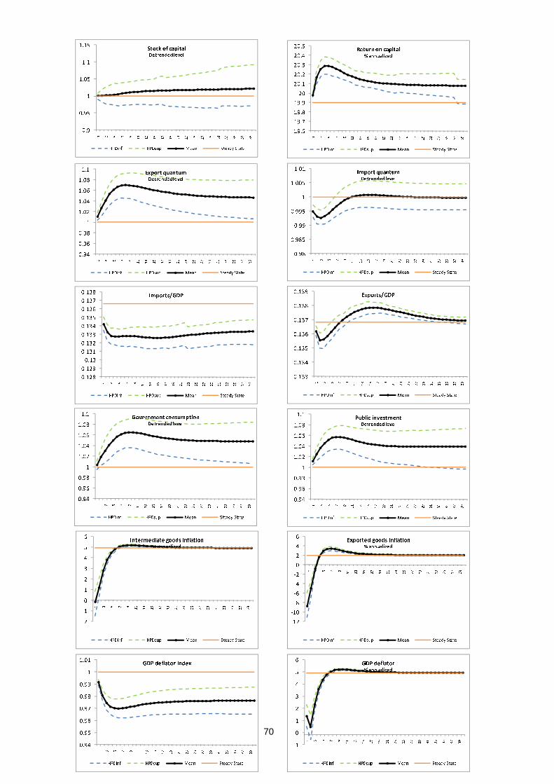
70
19.6
19.7
19.8
19.9
20
20.1
20.2
20.3
20.4
20.5
1 3 5 7 911
13
15
17
19
21
23
25
27
29
31
33
35
37
39
Return on capital% annualized
HPDinf HPDsup Mean Steady State
0.9
0.95
1
1.05
1.1
1.15
1 3 5 7 911
13
15
17
19
21
23
25
27
29
31
33
35
37
39
Stock of capitalDetrended level
HPDinf HPDsup Mean Steady State
0.98
0.985
0.99
0.995
1
1.005
1.01
1 3 5 7 911
13
15
17
19
21
23
25
27
29
31
33
35
37
39
Import quantumDetrended level
HPDinf HPDsup Mean Steady State
0.94
0.96
0.98
1
1.02
1.04
1.06
1.08
1.1
1 3 5 7 911
13
15
17
19
21
23
25
27
29
31
33
35
37
39
Export quantumDetrended level
HPDinf HPDsup Mean Steady State
0.133
0.134
0.135
0.136
0.137
0.138
0.139
1 3 5 7 911
13
15
17
19
21
23
25
27
29
31
33
35
37
39
Exports/GDP
HPDinf HPDsup Mean Steady State
0.128
0.129
0.13
0.131
0.132
0.133
0.134
0.135
0.136
0.137
0.138
1 3 5 7 911
13
15
17
19
21
23
25
27
29
31
33
35
37
39
Imports/GDP
HPDinf HPDsup Mean Steady State
0.94
0.96
0.98
1
1.02
1.04
1.06
1.08
1.1
1 3 5 7 911
13
15
17
19
21
23
25
27
29
31
33
35
37
39
Public investmentDetrended level
HPDinf HPDsup Mean Steady State
0.94
0.96
0.98
1
1.02
1.04
1.06
1.08
1.1
1 3 5 7 911
13
15
17
19
21
23
25
27
29
31
33
35
37
39
Government consumptionDetrended level
HPDinf HPDsup Mean Steady State
0.94
0.95
0.96
0.97
0.98
0.99
1
1.01
1 3 5 7 911
13
15
17
19
21
23
25
27
29
31
33
35
37
39
GDP deflator index
HPDinf HPDsup Mean Steady State
-1
0
1
2
3
4
5
6
1 3 5 7 911
13
15
17
19
21
23
25
27
29
31
33
35
37
39
GDP deflator % annualized
HPDinf HPDsup Mean Steady State
-2
-1
0
1
2
3
4
5
6
1 3 5 7 911
13
15
17
19
21
23
25
27
29
31
33
35
37
39
Intermediate goods inflation% annualized
HPDinf HPDsup Mean Steady State
-12
-10
-8
-6
-4
-2
0
2
4
6
1 3 5 7 911
13
15
17
19
21
23
25
27
29
31
33
35
37
39
Exported goods inflation% annualized
HPDinf HPDsup Mean Steady State

71
Figure 15: Impulse responses to a 1 s.d. permanent (labor-augmenting)
productivity shock
0
2
4
6
8
10
12
14
16
18Nominal Interest Rate
% annualized
HPDinf HPDsup Mean Steady State
0
2
4
6
8
10
12CPI inflation rate
% annualized
HPDinf HPDsup Mean Steady State
0
0.2
0.4
0.6
0.8
1
1.2
1.4
1.6Output
Detrended level
HPDinf HPDsup Mean Steady State
0
5
10
15
20
25
30Output growth
% annualized
HPDinf HPDsup Mean Steady State
0
0.2
0.4
0.6
0.8
1
1.2
1.4
1.6
1.8
2
1 3 5 7 911
13
15
17
19
21
23
25
27
29
31
33
35
37
39
Nominal exchange rate Detrended level
HPDinf HPDsup Mean Steady State
0
0.5
1
1.5
2
2.5
3
3.5
1 3 5 7 911
13
15
17
19
21
23
25
27
29
31
33
35
37
39
Public debt/GDP
HPDinf HPDsup Mean Steady State
0
0.005
0.01
0.015
0.02
0.025
0.03
0.035
0.04
1 3 5 7 911
13
15
17
19
21
23
25
27
29
31
33
35
37
39
Primary surplus/GDP
HPDinf HPDsup Mean Steady State
0.154
0.156
0.158
0.16
0.162
0.164
0.166
0.168
1 3 5 7 911
13
15
17
19
21
23
25
27
29
31
33
35
37
39
Government consumption/GDP
HPDinf HPDsup Mean Steady State
0
0.2
0.4
0.6
0.8
1
1.2
1.4
1.6
1.8
1 3 5 7 911
13
15
17
19
21
23
25
27
29
31
33
35
37
39
Private consumptionDetrended level
HPDinf HPDsup Mean Steady State
0
0.2
0.4
0.6
0.8
1
1.2
1.4
1.6
1 3 5 7 911
13
15
17
19
21
23
25
27
29
31
33
35
37
39
Real wagesDetrended level
HPDinf HPDsup Mean Steady State

72
19.4
19.6
19.8
20
20.2
20.4
20.6
20.8
21
1 3 5 7 911
13
15
17
19
21
23
25
27
29
31
33
35
37
39
Return on capital% annualized
HPDinf HPDsup Mean Steady State
0
0.2
0.4
0.6
0.8
1
1.2
1 3 5 7 911
13
15
17
19
21
23
25
27
29
31
33
35
37
39
Stock of capitalDetrended level
HPDinf HPDsup Mean Steady State
0
0.2
0.4
0.6
0.8
1
1.2
1.4
1.6
1 3 5 7 911
13
15
17
19
21
23
25
27
29
31
33
35
37
39
Import quantumDetrended level
HPDinf HPDsup Mean Steady State
0
0.2
0.4
0.6
0.8
1
1.2
1.4
1.6
1 3 5 7 911
13
15
17
19
21
23
25
27
29
31
33
35
37
39
Export quantumDetrended level
HPDinf HPDsup Mean Steady State
0.12
0.125
0.13
0.135
0.14
0.145
1 3 5 7 911
13
15
17
19
21
23
25
27
29
31
33
35
37
39
Exports/GDP
HPDinf HPDsup Mean Steady State
0.115
0.12
0.125
0.13
0.135
0.14
0.145
1 3 5 7 911
13
15
17
19
21
23
25
27
29
31
33
35
37
39
Imports/GDP
HPDinf HPDsup Mean Steady State
0
0.2
0.4
0.6
0.8
1
1.2
1.4
1.6
1 3 5 7 911
13
15
17
19
21
23
25
27
29
31
33
35
37
39
Public investmentDetrended level
HPDinf HPDsup Mean Steady State
0
0.2
0.4
0.6
0.8
1
1.2
1.4
1.6
1 3 5 7 911
13
15
17
19
21
23
25
27
29
31
33
35
37
39
Government consumptionDetrended level
HPDinf HPDsup Mean Steady State
0.94
0.96
0.98
1
1.02
1.04
1.06
1.08GDP deflator index
HPDinf HPDsup Mean Steady State
0
2
4
6
8
10
12
14
1 3 5 7 911
13
15
17
19
21
23
25
27
29
31
33
35
37
39
GDP deflator % annualized
HPDinf HPDsup Mean Steady State
0
1
2
3
4
5
6
7
8Intermediate goods inflation
% annualized
HPDinf HPDsup Mean Steady State
-30
-25
-20
-15
-10
-5
0
5
1 3 5 7 911
13
15
17
19
21
23
25
27
29
31
33
35
37
39
Exported goods inflation% annualized
HPDinf HPDsup Mean Steady State

73
Figure 16: Historical Shock Decomposition (main shocks)
-0.03
-0.02
-0.01
0
0.01
0.02
0.03
Mar-99
Sep-99
Mar-00
Sep-00
Mar-01
Sep-01
Mar-02
Sep-02
Mar-03
Sep-03
Mar-04
Sep-04
Mar-05
Sep-05
Mar-06
Sep-06
Mar-07
Sep-07
Mar-08
Sep-08
Mar-09
Sep-09
Mar-10
Nominal Interest Rate
er ez ezn erp emkp erzn
total factor (temporary) productivity
domestic risk premium
permanent
(labor-
augmenting)
differential to foreign productivity
price markup
monetary policy
-4%
-3%
-2%
-1%
0%
1%
2%
3%
4%
5%
Mar-99
Sep-99
Mar-00
Sep-00
Mar-01
Sep-01
Mar-02
Sep-02
Mar-03
Sep-03
Mar-04
Sep-04
Mar-05
Sep-05
Mar-06
Sep-06
Mar-07
Sep-07
Mar-08
Sep-08
Mar-09
Sep-09
Mar-10
CPI
emkp
erp
ezn
ez
domestic risk premium
Price markup
Temporary
productivity
permanent (labor-
augmenting)
productivity

74
-0.06
-0.04
-0.02
0
0.02
0.04
0.06
0.08
Mar-99
Sep-99
Mar-00
Sep-00
Mar-01
Sep-01
Mar-02
Sep-02
Mar-03
Sep-03
Mar-04
Sep-04
Mar-05
Sep-05
Mar-06
Sep-06
Mar-07
Sep-07
Mar-08
Sep-08
Mar-09
Sep-09
Mar-10
Primary Surplus/GDP
erp
eig
esp
ezn
ez
permanent (labor-augmenting) productivity
temporary productivity
primary-surplus shock
domestic risk premium
public investment
-0.1
-0.05
0
0.05
0.1
0.15
0.2
Mar-99
Sep-99
Mar-00
Sep-00
Mar-01
Sep-01
Mar-02
Sep-02
Mar-03
Sep-03
Mar-04
Sep-04
Mar-05
Sep-05
Mar-06
Sep-06
Mar-07
Sep-07
Mar-08
Sep-08
Mar-09
Sep-09
Mar-10
Consumption/GDP
ez ezn etr eig erp
public investment
permanent (labor-augmenting) productivity
temporary productivity
domestic risk premium
public transfers
public
transfers

75
Figure 17: Policy Exercise – Changing the Primary Surplus Target: Shock to the
Monetary Policy Rule
Figure 18: Policy Exercise – Changing the Reaction to the Debt-to-GDP Ratio in
the Fiscal Rule for the Primary Surplus: Shock to the Primary Surplus Rule
4
4.1
4.2
4.3
4.4
4.5
4.6
4.7
4.8
4.9
5
1 3 5 7 911
13
15
17
19
21
23
25
27
29
31
33
35
37
39
CPI inflation rate% annualized
Primary Surplus Target=1.5% of GDP
Primary Surplus Target=3.4% of GDP
Steady State
12.5
13
13.5
14
14.5
15
1 3 5 7 911
13
15
17
19
21
23
25
27
29
31
33
35
37
39
Nominal Interest Rate% annualized
Primary Surplus Target=1.5% of GDP
Primary Surplus Target=3.4% of GDP
Steady State
0.99
0.992
0.994
0.996
0.998
1
1 3 5 7 911
13
15
17
19
21
23
25
27
29
31
33
35
37
39
Output Detrended level
Primary Suprlus Target=1.5% of GDP
Primary Surplus Target=3.4% of GDP
Steady State
1
1.5
2
2.5
3
3.5
1 3 5 7 911
13
15
17
19
21
23
25
27
29
31
33
35
37
39
Public debt/GDP
Primary Suprlus Target=1.5% of GDP
Primary Surplus Target=3.4% of GDP
Steady State
4
4.2
4.4
4.6
4.8
5
5.2
5.4
5.6
5.8
6
1 3 5 7 911
13
15
17
19
21
23
25
27
29
31
33
35
37
39
CPI inflation rate% annualized
coefficient=0.20 coefficient=0.10
Estimated Mean (coefficient=0.017) Steady State
0.92
0.94
0.96
0.98
1
1.02
1.04
1 3 5 7 911
13
15
17
19
21
23
25
27
29
31
33
35
37
39
Output Detrended level
coefficient=0.20 coefficient=0.10
Estimated Mean (coefficient=0.017) Steady State
2.85
2.9
2.95
3
3.05
3.1
3.15
3.2
1 3 5 7 911
13
15
17
19
21
23
25
27
29
31
33
35
37
39
Public debt/GDP
coefficient=0.20 coefficient=0.10
Estimated Mean (coefficient=0.017) Steady State
0
0.01
0.02
0.03
0.04
0.05
0.06
1 3 5 7 911
13
15
17
19
21
23
25
27
29
31
33
35
37
39
Primary surplus/GDP
coefficient=0.20 coefficient=0.10
Estimated Mean (coefficient=0.017) Steady State

76
Figure 19: Policy Exercise – Changing the Reaction to GDP Growth in the Fiscal
Rule for the Primary Surplus: Shock to the Primary Surplus Rule
4.8
4.85
4.9
4.95
5
5.05
5.1
5.15
5.2
5.25
5.3
1 3 5 7 911
13
15
17
19
21
23
25
27
29
31
33
35
37
39
CPI inflation rate% annualized
coefficient=0.50 coefficient=0.10
Estimated Mean (coefficient=0.038) Steady State
0.98
0.985
0.99
0.995
1
1.005
1.01
1.015
1.02
1.025
1.03
1 3 5 7 911
13
15
17
19
21
23
25
27
29
31
33
35
37
39
Output Detrended level
coefficient=0.50 coefficient=0.10
Estimated Mean (coefficient=0.038) Steady State
2.98
3
3.02
3.04
3.06
3.08
3.1
3.12
3.14
1 3 5 7 911
13
15
17
19
21
23
25
27
29
31
33
35
37
39
Public debt/GDP
coefficient=0.50 coefficient=0.10
Estimated Mean (coefficient=0.038) Steady State
0.01
0.015
0.02
0.025
0.03
0.035
0.04
1 3 5 7 911
13
15
17
19
21
23
25
27
29
31
33
35
37
39
Primary surplus/GDP
coefficient=0.50 coefficient=0.10
Estimated Mean (coefficient=0.038) Steady State
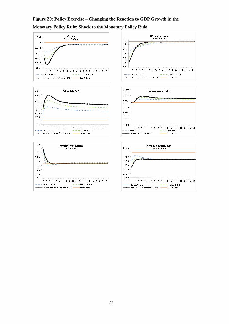
77
Figure 20: Policy Exercise – Changing the Reaction to GDP Growth in the
Monetary Policy Rule: Shock to the Monetary Policy Rule
3.8
4
4.2
4.4
4.6
4.8
5
1 3 5 7 911
13
15
17
19
21
23
25
27
29
31
33
35
37
39
CPI inflation rate% annualized
coefficient=0.70 coefficient=0.20
Estimated Mean (coefficient=0.023) Steady State
0.99
0.992
0.994
0.996
0.998
1
1.002
1 3 5 7 911
13
15
17
19
21
23
25
27
29
31
33
35
37
39
Output Detrended level
coefficient=0.70 coefficient=0.20
Estimated Mean (coefficient=0.023) Steady State
3.06
3.07
3.08
3.09
3.1
3.11
3.12
3.13
3.14
3.15
1 3 5 7 911
13
15
17
19
21
23
25
27
29
31
33
35
37
39
Public debt/GDP
coefficient=0.70 coefficient=0.20
Estimated Mean (coefficient=0.023) Steady State
0.03
0.031
0.032
0.033
0.034
0.035
0.036
1 3 5 7 911
13
15
17
19
21
23
25
27
29
31
33
35
37
39
Primary surplus/GDP
coefficient=0.70 coefficient=0.20
Estimated Mean (coefficient=0.023) Steady State
11
11.5
12
12.5
13
13.5
14
14.5
15
1 3 5 7 911
13
15
17
19
21
23
25
27
29
31
33
35
37
39
Nominal Interest Rate% annualized
coefficient=0.70 coefficient=0.20
Estimated Mean (coefficient=0.023) Steady State
0.97
0.975
0.98
0.985
0.99
0.995
1
1.005
1 3 5 7 911
13
15
17
19
21
23
25
27
29
31
33
35
37
39
Nominal exchange rate Detrended level
coefficient=0.70 coefficient=0.20
Estimated Mean (coefficient=0.023) Steady State

78
Figure 21: Policy Exercise – Changing the Size (�) of the Worse-off Share of the Population: Shock to the Primary Surplus Rule
� � �. �� � � �. �� � � �. ���
0.994
0.996
0.998
1
1.002
1.004
1.006
1.008
1.01
1 3 5 7 911
13
15
17
19
21
23
25
27
29
31
33
35
37
39
Private consumptionDetrended level
Mean Steady State
0.998
0.9985
0.999
0.9995
1
1.0005
1 3 5 7 911
13
15
17
19
21
23
25
27
29
31
33
35
37
39
Real wagesDetrended level
Mean Steady State
0.994
0.996
0.998
1
1.002
1.004
1.006
1.008
1.01
1 3 5 7 911
13
15
17
19
21
23
25
27
29
31
33
35
37
39
Private consumptionDetrended level
Mean Steady State
0.998
0.9985
0.999
0.9995
1
1.0005
1 3 5 7 911
13
15
17
19
21
23
25
27
29
31
33
35
37
39
Real wagesDetrended level
Mean Steady State
0.994
0.996
0.998
1
1.002
1.004
1.006
1.008
1.01
1 3 5 7 911
13
15
17
19
21
23
25
27
29
31
33
35
37
39
Private consumptionDetrended level
Mean Steady State
0.998
0.9985
0.999
0.9995
1
1.0005
1 3 5 7 911
13
15
17
19
21
23
25
27
29
31
33
35
37
39
Real wagesDetrended level
Mean Steady State

79
Banco Central do Brasil
Trabalhos para Discussão Os Trabalhos para Discussão do Banco Central do Brasil estão disponíveis para download no website
http://www.bcb.gov.br/?TRABDISCLISTA
Working Paper Series
The Working Paper Series of the Central Bank of Brazil are available for download at http://www.bcb.gov.br/?WORKINGPAPERS
203 Hiato do Produto e PIB no Brasil: uma Análise de Dados em
Tempo Real Rafael Tiecher Cusinato, André Minella e Sabino da Silva Pôrto Júnior
Abr/2010
204 Fiscal and monetary policy interaction: a simulation based analysis of a two-country New Keynesian DSGE model with heterogeneous households Marcos Valli and Fabia A. de Carvalho
Apr/2010
205 Model selection, estimation and forecasting in VAR models with short-run and long-run restrictions George Athanasopoulos, Osmani Teixeira de Carvalho Guillén, João Victor Issler and Farshid Vahid
Apr/2010
206 Fluctuation Dynamics in US interest rates and the role of monetary policy Daniel Oliveira Cajueiro and Benjamin M. Tabak
Apr/2010
207 Brazilian Strategy for Managing the Risk of Foreign Exchange Rate Exposure During a Crisis Antonio Francisco A. Silva Jr.
Apr/2010
208 Correlação de default: uma investigação empírica de créditos de varejo no Brasil Antonio Carlos Magalhães da Silva, Arnildo da Silva Correa, Jaqueline Terra Moura Marins e Myrian Beatriz Eiras das Neves
Maio/2010
209 Produção Industrial no Brasil: uma análise de dados em tempo real Rafael Tiecher Cusinato, André Minella e Sabino da Silva Pôrto Júnior
Maio/2010
210 Determinants of Bank Efficiency: the case of Brazil Patricia Tecles and Benjamin M. Tabak
May/2010
211 Pessimistic Foreign Investors and Turmoil in Emerging Markets: the case of Brazil in 2002 Sandro C. Andrade and Emanuel Kohlscheen
Aug/2010
212 The Natural Rate of Unemployment in Brazil, Chile, Colombia and Venezuela: some results and challenges Tito Nícias Teixeira da Silva
Sep/2010

80
213 Estimation of Economic Capital Concerning Operational Risk in a Brazilian banking industry case Helder Ferreira de Mendonça, Délio José Cordeiro Galvão and Renato Falci Villela Loures
Oct/2010
214 Do Inflation-linked Bonds Contain Information about Future Inflation? José Valentim Machado Vicente and Osmani Teixeira de Carvalho Guillen
Oct/2010
215 The Effects of Loan Portfolio Concentration on Brazilian Banks’ Return and Risk Benjamin M. Tabak, Dimas M. Fazio and Daniel O. Cajueiro
Oct/2010
216 Cyclical Effects of Bank Capital Buffers with Imperfect Credit Markets:
international evidence A.R. Fonseca, F. González and L. Pereira da Silva
Oct/2010
217 Financial Stability and Monetary Policy – The case of Brazil
Benjamin M. Tabak, Marcela T. Laiz and Daniel O. Cajueiro Oct/2010
218 The Role of Interest Rates in the Brazilian Business Cycles
Nelson F. Souza-Sobrinho
Oct/2010
219 The Brazilian Interbank Network Structure and Systemic Risk Edson Bastos e Santos and Rama Cont
Oct/2010
220 Eficiência Bancária e Inadimplência: testes de Causalidade Benjamin M. Tabak, Giovana L. Craveiro e Daniel O. Cajueiro
Out/2010
221 Financial Instability and Credit Constraint: evidence from the cost of bank financing Bruno S. Martins
Nov/2010
222 O Comportamento Cíclico do Capital dos Bancos Brasileiros R. A. Ferreira, A. C. Noronha, B. M. Tabak e D. O. Cajueiro
Nov/2010
223 Forecasting the Yield Curve with Linear Factor Models Marco Shinobu Matsumura, Ajax Reynaldo Bello Moreira and José Valentim Machado Vicente
Nov/2010
224 Emerging Floaters: pass-throughs and (some) new commodity currencies Emanuel Kohlscheen
Nov/2010
225 Expectativas Inflacionárias e Inflação Implícita no Mercado Brasileiro Flávio de Freitas Val, Claudio Henrique da Silveira Barbedo e Marcelo Verdini Maia
Nov/2010
226 A Macro Stress Test Model of Credit Risk for the Brazilian Banking Sector Francisco Vazquez, Benjamin M.Tabak and Marcos Souto
Nov/2010
227 Uma Nota sobre Erros de Previsão da Inflação de Curto Prazo Emanuel Kohlscheen
Nov/2010
228 Forecasting Brazilian Inflation Using a Large Data Set Francisco Marcos Rodrigues Figueiredo
Dec/2010
229 Financial Fragility in a General Equilibrium Model: the Brazilian case Benjamin M. Tabak, Daniel O. Cajueiro and Dimas M. Fazio
Dec/2010

81
230 Is Inflation Persistence Over? Fernando N. de Oliveira and Myrian Petrassi
Dec/2010
231 Capital Requirements and Business Cycles with Credit Market Imperfections P. R. Agénor, K. Alper and L. Pereira da Silva
Jan/2011
232 Modeling Default Probabilities: the case of Brazil Benjamin M. Tabak, Daniel O. Cajueiro and A. Luduvice
Jan/2011
233 Emerging Floaters: pass-throughs and (some) new commodity currencies Emanuel Kohlscheen
Jan/2011
234 Cyclical Effects of Bank Capital Requirements with Imperfect Credit Markets Pierre-Richard Agénor and Luiz A. Pereira da Silva
Jan/2011
235 Revisiting bank pricing policies in Brazil: Evidence from loan and deposit markets Leonardo S. Alencar
Mar/2011
236 Optimal costs of sovereign default Leonardo Pio Perez
Apr/2011
237 Capital Regulation, Monetary Policy and Financial Stability P.R. Agénor, K. Alper, and L. Pereira da Silva
Apr/2011
238 Choques não Antecipados de Política Monetária e a Estrutura a Termo das Taxas de Juros no Brasil Fernando N. de Oliveira e Leonardo Ramos
Abr/2011
239 SAMBA: Stochastic Analytical Model with a Bayesian Approach Marcos R. de Castro, Solange N. Gouvea, André Minella, Rafael C. Santos and Nelson F. Souza-Sobrinho
Apr/2011